ada compliant lecture powerpoint - yulin hou...title ada compliant lecture powerpoint author paul m....

Copyright © 2017 Pearson Education, Inc. All Rights Reserved

Economics6th edition

Chapter 12 Firms in Perfectly Competitive

Markets

Modified by Yulin Hou

For Principles of Microeconomics

Florida International University

Fall 2017

1


Market structures

The market structures we will examine are, in decreasing order of

competitiveness:

• Perfectly competitive markets

• Monopolistically competitive markets

• Oligopolies

• Monopolies

Each market structure will be applicable to different real-world

markets, and will give us insight into how firms in certain types of

markets behave.

2


Discuss

The late Nobel prize—winning economist George Stigler once

wrote, “the most common and most important criticism of perfect

competition is that it is unrealistic”. Since few firm sell identical

products in markets where there are no barriers to entry, why do

economists believe that the model of perfect competition is

important?

Source: George Stigler, “Perfect Competition, Historically

Contemplated,” Journal of Political Economy, Vol. 65, February

1957, pp.1-17.

3


4


Perfectly Competitive Markets

Perfectly competitive market: one in which

• There are many buyers and sellers.

• All firms sell identical products.

• There are no barriers to new firms entering the market.

5


Perfectly competitive firms are price-takers: they are unable to

affect the market price.

This is because they are tiny relative to the market, and sell

exactly the same product as everyone else.

Example: Agricultural markets, like the market for wheat, are often

thought to be close to perfectly competitive.

6


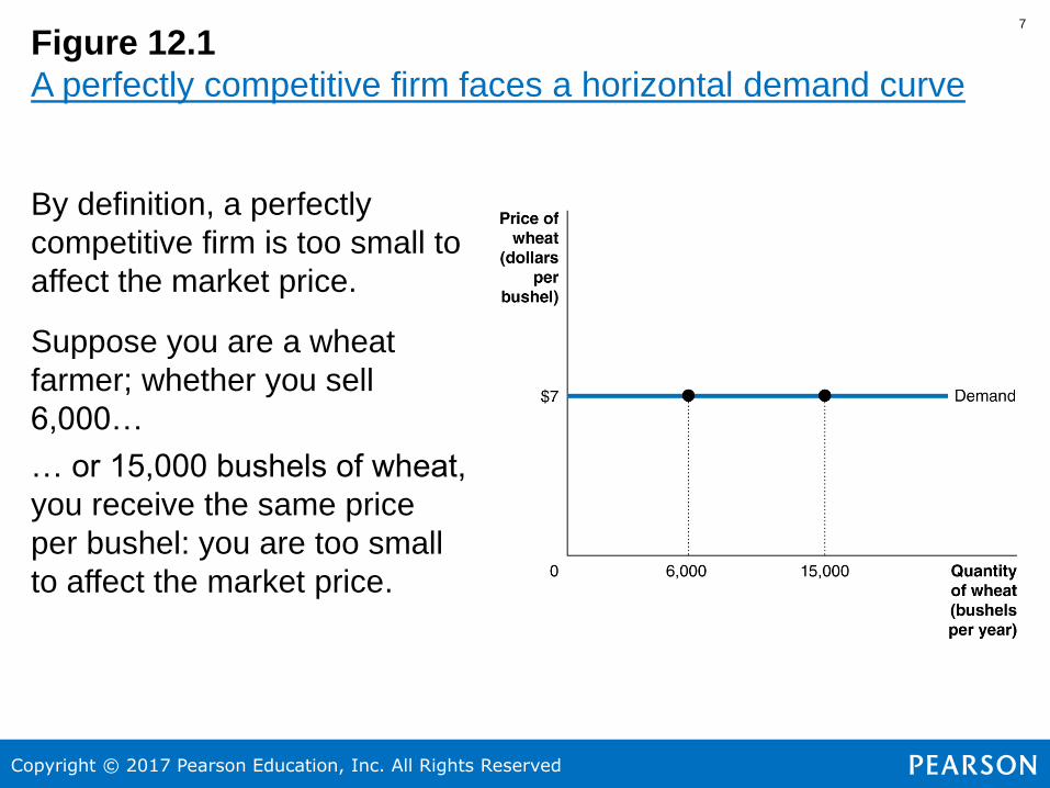
Figure 12.1

A perfectly competitive firm faces a horizontal demand curve

By definition, a perfectly

competitive firm is too small to

affect the market price.

Suppose you are a wheat

farmer; whether you sell

6,000…

… or 15,000 bushels of wheat,

you receive the same price

per bushel: you are too small

to affect the market price.

7


8


There are thousands of individual wheat farmers; their collective

supply, combined with the overall market demand for wheat,

determines the market price of wheat in the first panel.

The individual farmer takes this market price as his or her demand

curve: the second panel.

9


How a Firm Maximizes Profit in a

Perfect Competitive Market

We assume that all firms try to maximize. Recall that:

Profit = Total Revenue – Total Cost

Revenue for a perfectly competitive firm is easy: the firm receives

the same amount of money for every unit of output it sells. So:

𝐏𝐫𝐢𝐜𝐞 = 𝐀𝐯𝐞𝐫𝐚𝐠𝐞 𝐑𝐞𝐯𝐞𝐧𝐮𝐞 = 𝐌𝐚𝐫𝐠𝐢𝐧𝐚𝐥 𝐑𝐞𝐯𝐞𝐧𝐮𝐞

Average revenue (AR) is total revenue divided by the quantity of

the product sold

Marginal revenue (MR) is the change in total revenue from

selling one more unit of a product.

10


Table 12.2 Farmer Parker’s revenue from wheat farming

For a firm in a perfectly competitive market, price is equal to both

average revenue and marginal revenue:

𝑃 =𝑇𝑅

𝑄=∆𝑇𝑅

∆𝑄

11


Table 12.3 Farmer Parker’s profit from wheat farming

(1 of 2)

Suppose costs are as in the table.

We can calculate profit; profit is maximized at a quantity of 7

bushels. This is the profit-maximizing level of output.

12


Table 12.3 Farmer Parker’s profit from wheat farming

(2 of 2)

We can also calculate marginal revenue and marginal cost for the

firm.

Profit is maximized by producing as long as MR>MC; or until

MR=MC, if that is possible.

13


Figure 12.3 The profit-maximizing level of output (1 of 2)

If we show total revenue

and total cost on the

same graph, the vertical

difference between the

two curves is the profit

the firm makes.

• (Or the loss, if costs

are greater than

revenues.)

At the profit-maximizing

level of output, this

(positive) vertical

distance is maximized.

14


Figure 12.3 The profit-maximizing level of output (2 of 2)

It is generally easier to

determine the profit-

maximizing level of output

on a graph of marginal

revenue and marginal cost.

Marginal revenue is constant

and equal to price for the

perfectly competitive firm.

The firm maximizes profit by

choosing the level of output

where marginal revenue is

equal to marginal cost (or

just less, if equal is not

possible).

15


Rules for profit maximization

The rules we have just developed for profit maximization are:

1. The profit-maximizing level of output is where the difference

between total revenue and total cost is greatest; and

2. The profit-maximizing level of output is also where MR = MC.

However neither of these rules require the assumption of perfect

competition; they are true for every firm!

For perfectly competitive firms, we can develop an additional rule,

because for those firms, P = MR; this implies:

3. The profit-maximizing level of output is also where P = MC.

16


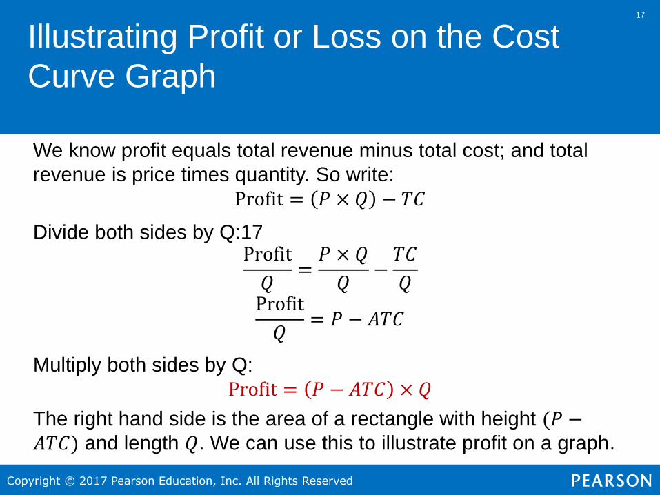
Illustrating Profit or Loss on the Cost

Curve Graph

We know profit equals total revenue minus total cost; and total

revenue is price times quantity. So write:

Profit = 𝑃 × 𝑄 − 𝑇𝐶

Divide both sides by Q:17Profit

𝑄=𝑃 × 𝑄

𝑄−𝑇𝐶

𝑄Profit

𝑄= 𝑃 − 𝐴𝑇𝐶

Multiply both sides by Q:

Profit = 𝑃 − 𝐴𝑇𝐶 × 𝑄

The right hand side is the area of a rectangle with height (𝑃 −𝐴𝑇𝐶) and length 𝑄. We can use this to illustrate profit on a graph.

17


The area of maximum profit (1 of 2)

A firm maximizes profit

at the level of output at

which marginal revenue

equals marginal cost.

The difference between

price and average total

cost equals profit per

unit of output.

Total profit equals profit

per unit of output, times

the amount of output: the

area of the green

rectangle on the graph.

18


The area of maximum profit (2 of 2)

Common error:

thinking profit is

maximized at Q1.

• This maximizes

profit per unit, but

NOT profit.

• The next few units

bring in more

marginal revenue

than their marginal

cost (MR > MC at

Q1); so they must

increase profit.

19


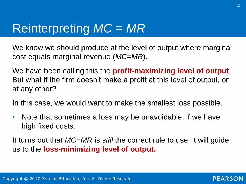
Reinterpreting MC = MR

We know we should produce at the level of output where marginal

cost equals marginal revenue (MC=MR).

We have been calling this the profit-maximizing level of output.

But what if the firm doesn’t make a profit at this level of output, or

at any other?

In this case, we would want to make the smallest loss possible.

• Note that sometimes a loss may be unavoidable, if we have

high fixed costs.

It turns out that MC=MR is still the correct rule to use; it will guide

us to the loss-minimizing level of output.

20


Example 1: A firm breaking even.

In the graph on the left, price

never exceeds average cost, so

the firm could not possibly

make a profit.

The best this firm can do is to

break even, obtaining no profit

but incurring no loss.

21


Example 2: A firm experiencing a loss.

The situation is even worse for

this firm; not only can it not

make a profit, price is always

lower than average total cost, so

it must make a loss.

It makes the smallest loss

possible by again following the

MC=MR rule. No other level of

output allows the firm’s loss to

be so small.

22


Identifying whether a firm can make a

profit

Step 1: Determined the quantity where MC=MR

Step 2: At that quantity,

• If P > ATC, the firm is making a profit

• If P = ATC, the firm is breaking even

• If P < ATC, the firm is making a loss

Even better: these statements hold true at every level of output.

23


“If Everyone Can Do It, You Can’t Make Money at

It”: The Entry and Exit of Firms in the Long Run

1.When firms in an industry are earning economic profits, new

firms will enter the industry.

2. When firms in an industry are suffering economic losses,

some of those firms will exit the industry.

24


Case 1: The effect of entry on economic profit

The profit attracts new firms, which increases supply.

25


Case 1: The effect of entry on economic profit

The increased supply causes the market equilibrium price to fall.

It falls until there is no incentive for further firms to enter the market;

that is, when individual firms make no economic profit.

26


Case 2: The effect of exit on economic losses

Price is $2 and firms are breaking even. Then the demand falls. The

demand curve shifts from D1 to D2. The price falls to $1.75.

27


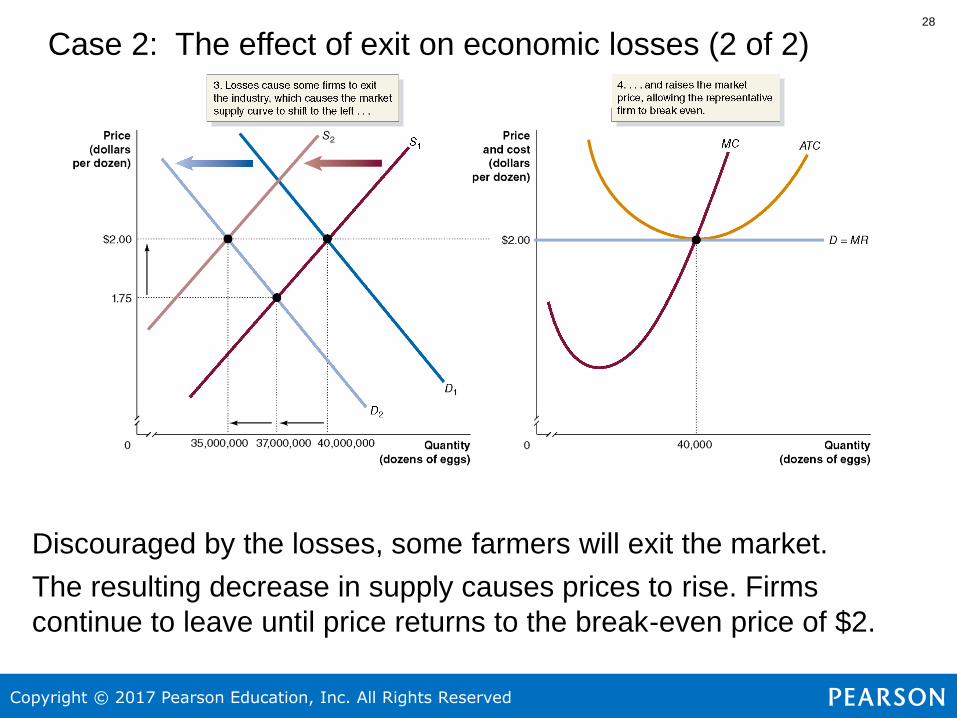
Case 2: The effect of exit on economic losses (2 of 2)

Discouraged by the losses, some farmers will exit the market.

The resulting decrease in supply causes prices to rise. Firms

continue to leave until price returns to the break-even price of $2.

28


Long-run equilibrium in a perfectly

competitive market

The previous slides have described how long-run competitive

equilibrium is achieved in a perfectly competitive market:

• If firms are making an economic profit, additional firms enter the

market, driving down price to the break-even level.

• If firms are making an economic loss, existing firms exit the

market, driving price up to the break-even level.

Long-run competitive equilibrium: The situation in which the

entry and exit of firms has resulted in the typical firm breaking

even.

29

ada compliant lecture powerpoint - yulin hou...title ada compliant lecture powerpoint author paul m....

Documents