Abstract

In bioengineering applications problems of flow interacting with elas-tic solid are very common. We formulate the problem of interaction foran incompressible fluid and an incompressible elastic material in a fullycoupled arbitrary Lagrangian-Eulerian formulation. The mathematicaldescription and the numerical schemes are designed in such a way thatmore complicated constitutive relations (and more realistic for bioengi-neering applications) can be incorporated easily. The whole domain ofinterest is treated as one continuum and the same discretization in space(Q2/P1 FEM) and time (Crank-Nicholson) is used for both, solid andfluid, parts. The resulting nonlinear algebraic system is solved by an ap-proximate Newton method. The combination of second order discretiza-tion and fully coupled solution method gives a method with high accuracyand robustness. To demonstrate the flexibility of this numerical approachwe apply the same method to a mixture based model of elastic materialwith perfusion which also falls into the category of fluid structure interac-tions. A few simple 2D example calculations with simple material modelsand a large deformations of the solid part are presented.

1

Fluid-structure interaction with applications in

biomechanics

J. Hron

University of Dortmund, Institute of Applied Mathematics,

Vogelpothsweg 87, 44227 Dortmund, Germany

1 Overview

Both problems of viscous fluid flow and of elastic body deformation have beenstudied separately for many years in great detail. But there are many problemsencountered in real life where an interaction between those two medias is of greatimportance. Typical example of such a problem is the area of aero-elasticity.Another important area where such interaction is of great interest is the biome-chanics. Such interaction is encountered especially when dealing with the bloodcirculatory system. Problem of a pulsative flow in an elastic tube, flow throughthe heart flaps, flow in the heart chambers are some of the examples. In all thesecases we have to deal with large deformations of a deformable solid interactingwith an unsteady, often periodic, fluid flow. The ability to model and predictthe mechanical behavior of biological tissues is very important in several areasof bio-engineering and medicine. For example, a good mathematical model forbiological tissue could be used in such areas as early recognition or predictionof heart muscle failure, advanced design of new treatments and operative proce-dures, and the understanding of atherosclerosis and associated problems. Otherpossible applications include development of virtual reality programs for train-ing new surgeons or designing new operative procedures (see Miga et al. [1998],Paulsen et al. [1999]), and last but not least the design of medical instrumentsor artificial replacements with optimal mechanical and other properties as closeas possible to the original parts (see Zoppou et al. [1997]). These are some ofthe areas where a good mathematical model of soft tissue with reliable and fastnumerical solution is essential for success.

1.1 Fluid structure models

There have been several different approaches to the problem of fluid-structureinteraction. Most notably the work of Peskin and McQueen [1989], Peskin[1982], Peskin and McQueen [1980], Peskin [1977] where an immersed boundarymethod was developed and applied to a three-dimensional model of the heart.In this model they consider a set of one-dimensional elastic fibers immersed

2

in three-dimensional fluid region and using parallel supercomputer they wereable to model the pulse of the heart ventricle. Their method can capture theanisotropy caused by the muscle fibers.

A fluid-structure model with the wall modeled as a thin shell was used tomodel the left heart ventricle in Costa et al. [1996a,b] and Quarteroni et al.[2000], Quarteroni [2001]. In Heil [1997, 1998] similar approach was used tomodel a flow in a collapsible tubes. In these models the wall is modeled bytwo-dimensional thin shell which can be modified to capture the anisotropy ofthe muscle. In reality the thickness of the wall can be significant and veryimportant. For example in arteries the wall thickness can be up to 30% of thediameter and its local thickening can be the cause of an aneurysm creation. Inthe case of heart ventricle the thickness of the wall is also significant and alsothe direction of the muscle fibers changes through the wall.

1.2 Mixture models for perfusion

Another class of models which fall into the fluid structure interaction problemsare the fluid-solid mixture models used for simulation of soft tissue perfusionlike muscles or cartelage. Mixture theory was first applied to swelling and dif-fusion in rubber materials Dai and Rajagopal [1990], Rajagopal and Tao [1995],mechanics of skin Oomens and van Campen [1987], compression of cartilageSpilker et al. [1988], Kwan et al. [1990], Reynolds and Humphrey [1998] andblood perfusion through biological tissues in Vankan et al. [1996, 1997]. (seefor example Fung [1993] and Maurel et al. [1998]) The basic idea of mixturetheory is the assumption of co-occupancy, i.e., at each spatial point there iscertain fraction of each constituent (with associated fields) and there are pre-scribed balance equations for each constituent of the mixture as is usual for asingle continuum, with additional terms representing the interaction betweenconstituents within the mixture.

There have been several numerical studies of mixture models. One dimen-sional diffusion of fluid through an isotropic material is solved in Shi [1973], fortransversely isotropic materials in Dai and Rajagopal [1990] and in Reynoldsand Humphrey [1998] a one dimensional diffusion through isotropic stretchedslab is solved using a velocity boundary condition. Finite element solutions ofmixture models for the small deformation, linear elastic case are presented inKwan et al. [1990], Vankan et al. [1997] and for nonlinear large deformationdescription of various soft tissues in Spilker et al. [1988], Spilker and Suh [1990],Suh et al. [1991], Donzelli et al. [1992], Vermilyea and Spilker [1993], Almeidaand Spilker [1998], Levenston et al. [1998].

1.3 Theoretical results

The theoretical investigation of the fluid structure interaction problems is com-plicated by the need of mixed description. While for the solid part the natu-ral view is the material (Lagrangian) description for the fluid it is the spatial

3

(Eulerian) description. In the case of their combination some kind of mixed de-scription (usually refered to as the arbitrary Lagrangian-Eulerian description)has to be used which brings additional nonlinearity into the resulting equations.

In Le Tallec and Mani [2000] a time dependent, linearized model of interac-tion between a viscous fluid and an elastic shell in small displacement approxi-mation and its discretization is analyzed. The problem is further simplified byneglecting all changes in the geometry configuration. Under these simplifica-tions by using the energy estimates they are able to show that the proposedformulation is well posed and a global weak solution exists. Further they showthat an independent discretization by standard mixed finite elements for thefluid and by nonconforming DKT finite elements for the shell together withbackward or central difference approximation of the time derivatives convergesto the solution of the continuous problem.

In Rumpf [1998] a steady problem of equilibrium of an elastic fixed obstaclesurrounded by a viscous fluid is studied. Existence of an equilibrium state isshow with the displacement and velocity in C2,α and pressure in C1,α underassumption of small data in C2,α and the domain boundaries of class C3.

For basic introduction and complete reference of continuum theory see Gurtin[1981], Truesdell [1991], Marsık [1999], Haupt [2000]. Its application in biome-chanics are presented in Fung [1993] and Marsık and Dvorak [1998] for example.We will mention in the following sections the basic notation and setup used inthis work.

A numerical solution of the resulting equations of the fluid structure inter-action problem poses great challenge since it includes the features of nonlinearelasticity, fluid mechanics and their coupling. The easiest solution strategy,mostly used in the available software packages, is to decouple the problem intothe fluid part and solid part, for each of those parts to use some well establishedmethod of solution then the interaction is introduced as external boundary con-ditions in each of the subproblems. This has an advantage that there are manywell tested finite element based numerical methods for separate problems offluid flow and elastic deformation, on the other hand the treatment of the in-terface and the interaction is problematic. The approach presented here treatsthe problem as a single continuum with the coupling automatically taken careof as internal interface, which in our formulation does not require any specialtreatment.

2 Continuum description

Let Ω ⊂ R3 be a reference configuration of a given body, possibly an abstract

one. Let Ωt ⊂ R3 be a configuration of this body at time t. Then one-to-one,

sufficiently smooth mapping χΩ of the reference configuration Ω to the currentconfiguration

χΩ : Ω × [0, T ] 7→ Ωt, (1)

4

Ω0 Ωt

Ω

χΩ0(t)

χΩ(t)χΩ(0)

Figure 1: The referential domain Ω, initial Ω0 and current state Ωt and relationsbetween them. The identification Ω ≡ Ω0 is adopted in this text.

describes the motion of the body, see figure 1. The mapping χΩ depends on thechoice of the reference configuration Ω which can be fixed in a various ways.Here we think of Ω to be the initial (stress-free) configuration Ω0. Thus, if notemphasized, we mean by χ exactly χΩ = χΩ0

.If we denote by X a material point in the reference configuration Ω then the

position of this point at time t is given by

x = χ(X, t). (2)

Next, the mechanical fields describing the deformation are defined in a standardmanner. The displacement field, the velocity field, deformation gradient and itsdeterminant as

u(X, t) = χ(X, t) − X, v =∂χ

∂t, F =

∂χ

∂X, J = detF . (3)

Let us adopt following useful notations for some derivatives. Any field quantityϕ with values in some vector space Y (i.e. scalar, vector or tensor valued) canbe expressed in the Eulerian description as a function of the spatial positionx ∈ R

3

ϕ = ϕ(x, t) : Ωt × [0, T ] 7→ Y.

Then we define following notations for the derivatives of the field ϕ

∂ϕ

∂t:=

∂ϕ

∂t, ∇ϕ =

∂ϕ

∂x:=

∂ϕ

∂x, div ϕ := tr∇ϕ. (4)

In the case of Lagrangian description we consider the quantity ϕ to be defined onthe reference configuration Ω, then for any X ∈ Ω we can express the quantityϕ as

ϕ = ϕ(X, t) : Ω × [0, T ] 7→ Y,

5

and we define the derivatives of the field ϕ as

dϕ

dt:=

∂ϕ

∂t, Gradϕ =

∂ϕ

∂X:=

∂ϕ

∂X, Div ϕ := trGradϕ. (5)

These two descriptions can be related to each other through following relations

ϕ(X, t) =ϕ(χ(X, t), t), (6)

dϕ

dt=

∂ϕ

∂t+ (∇ϕ)v, Gradϕ =(∇ϕ)F ,

∫

Ωt

ϕdv =

∫

Ω

ϕJdV (7)

dF

dt= Gradv,

∂J

∂F=JF

−T ,dJ

dt=J div v. (8)

For the formulation of the balance laws we will need to express a time deriva-tives of some integrals. The following series of equalities obtained by using thepreviously stated relations will be useful

d

dt

∫

Ωt

ϕdv =d

dt

∫

Ω

ϕJdV =

∫

Ω

d

dt(ϕJ) dV =

∫

Ωt

(

dϕ

dt+ ϕdiv v

)

dv

=

∫

Ωt

(

∂ϕ

∂t+ div (ϕv)

)

dv =

∫

Ωt

∂ϕ

∂tdv +

∫

∂Ωt

ϕv · nda

=∂

∂t

∫

Ωt

ϕdv +

∫

∂Ωt

ϕv · nda.

(9)

And also the Piola identity will be used Div(JF−T ) = 0, which can be checked

by differentiating the left hand side and using (8) together with an identityobtained by differentiating the relation FF

−1 = I.

2.1 Balance laws

In this section we will formulate the balance relations for mass and momen-tum in three forms: the Eulerian, the Lagrangian and the arbitrary Eulerian-Lagrangian (ALE) description.

The Eulerian (or spatial) description is well suited for a problem of fluidflowing through some spatially fixed region. In such a case the material particlescan enter and leave the region of interest. The fundamental quantity describingthe motion is the velocity vector.

On the other hand the Lagrangian (or referential) description is well suitedfor a problem of deforming a given body consisting of a fixed set of materialparticles. In this case the actual boundary of the body can change its shape.The fundamental quantity describing the motion in this case is the vector ofdisplacement from the referential state.

In the case of fluid-structure interaction problem we can still use the La-grangian description for the deformation of the solid part. The fluid flow nowtakes place in a domain with boundary given by the deformation of the struc-ture which can change in time and is influenced back by the fluid flow. The

6

mixed ALE description of the fluid has to be used in this case. The fundamen-tal quantity describing the motion of the fluid is still the velocity vector but thedescription is accompanied by a certain displacement field which describes thechange of the fluid domain. This displacement field has no connection to thefluid velocity field and the purpose of its introduction is to provide a transfor-mation of the current fluid domain and corresponding governing equations tosome fixed reference domain. This method is sometimes called a pseudo-solidmapping method [see Sackinger et al., 1996].

Let P ⊂ R3 be a fixed region in space (control volume) with the boundary

∂P and unit outward normal vector nP , such that

P ⊂ Ωt for all t ∈ [0, T ].

Let denotes the mass density of the material. Then the balance of mass inthe region P can be written as

∂

∂t

∫

P

dv +

∫

∂P

v · nPda = 0. (10)

If all the fields are sufficiently smooth this equation can be written in local formwith respect to the current configuration as

∂

∂t+ div(v) = 0. (11)

It will be useful to derive the mass balance equation from the Lagrangian pointof view. Let Q ⊂ Ω be a fixed set of particles. Then χ(Q, t) ⊂ Ωt is a re-gion occupied by these particles at the time t, and the balance of mass can beexpressed as

d

dt

∫

χ(Q,t)

dv = 0, (12)

which in local form with respect to the reference configuration can be writtenas

d

dt(J) = 0. (13)

In the case of arbitrary Lagrangian-Eulerian description we take a regionZ ⊂ R

3 which is itself moving independently of the motion of the body. Let themotion of the control region Z be described by a given mapping

ζZ : Z × [0, T ] 7→ Zt, Zt ⊂ Ωt ∀t ∈ [0, T ],

with the corresponding velocity vZ = ∂ζZ∂t

, deformation gradient FZ = ∂ζZ∂X

andits determinant JZ = detFZ . The mass balance equation can be written as

∂

∂t

∫

Zt

dv +

∫

∂Zt

(v − vZ) · nZtda = 0, (14)

7

this can be viewed as Eulerian description with moving spatial coordinate systemor as a grid deformation in the context of the finite element method. In order toobtain a local form of the balance relation we need to transform the integrationto the fixed spatial region Z

∂

∂t

∫

Z

JZdv +

∫

∂Z

(v − vZ) · F−TZ nZJZda = 0, (15)

then the local form is

∂

∂t(JZ) + div

(

JZ(v − vZ)F−TZ

)

= 0. (16)

The two previous special formulations can be now recovered. If the region Zis not moving in space, i.e. Z = Zt, ∀t ∈ [0, T ], then ζZ is the identity mapping,FZ = I, JZ = 1,vZ = 0 and (16) reduces to (11). While, if the region Z movesexactly with the material, i.e. ζZ = χ|Z then FZ = F , JZ = J,vZ = v and(16) reduces to (13).

The balance of linear momentum is postulated in a similar way. Let σ denotethe Cauchy stress tensor field, representing the surface forces per unit area, f

be the body forces acting on the material per its unit mass. Then the balanceof linear momentum in the Eulerian description is stated as

∂

∂t

∫

P

vdv +

∫

∂P

v ⊗ vnPda =

∫

∂P

σTnPda +

∫

P

fdv. (17)

The local form of the linear momentum balance is

∂v

∂t+ div(v ⊗ v) = div σ

T + f , (18)

or with the use of (11) we can write

∂v

∂t+ (∇v)v = div σ

T + f . (19)

From the Lagrangian point of view the momentum balance relation is

d

dt

∫

χ(Q,t)

vdv =

∫

∂χ(Q,t)

σTnχ(Q,t)da +

∫

χ(Q,t)

fdv. (20)

Let us denote by P = JσTF

−T the first Piola-Kirchhoff stress tensor [seeGurtin, 1981], then the local form of the momentum balance is

d

dt(Jv) = Div P + Jf , (21)

or using (13) we can write

Jdv

dt= Div P + Jf . (22)

8

In the arbitrary Lagrangian-Eulerian formulation we obtain

∂

∂t

∫

Zt

vdv +

∫

∂Zt

v ⊗ (v − vZ)nZtda =

∫

∂Zt

σTnZt

da +

∫

Zt

fdv, (23)

which in the local form gives

∂JZv

∂t+ div

(

JZv ⊗ (v − vZ)F−TZ

)

= div(

JZσTF

−TZ

)

+ JZf , (24)

or with the use of (16) we can write

JZ

∂v

∂t+ JZ(∇v)F −T

Z (v − vZ) = div(

JZσTF

−TZ

)

+ JZ f . (25)

In the case of angular momentum balance we assume that there are noexternal or internal sources of angular momentum, then it follows that theCauchy stress tensor has to be symmetric, i.e. σ = σT . Assuming an isothermalconditions the energy balance is satisfied and the choice of the constitutiverelations for the materials has to be compatible with the balance of entropy.[see Truesdell, 1991]

3 Fluid structure interaction problem formula-

tion

At this point we make a few assumptions that will allow us to deal with thetask of setting up a tractable problem. We will use the superscripts s and f todenote the quantities connected with the solid and fluid. Let us assume that theboth materials are incompressible and all the processes are isothermal, whichis well accepted approximation in biomechanics and let us denote the constantdensities of each material by f , s.

3.1 Monolithic description

We denote by Ωft the domain occupied by the fluid and Ωs

t by the solid at time

t ∈ [0, T ]. Let Γ0t = Ωf

t ∩ Ωst be the part of the boundary where the solid

interacts with the fluid and Γit, i = 1, 2, 3 be the remaining external boundaries

of the solid and the fluid as depicted in figure 2.Let the deformation of the solid part be described by the mapping χs

χs : Ωs × [0, T ] 7→ Ωst , (26)

with the corresponding displacement us and the velocity v

s given by

us(X, t) = χs(X, t) − X, v

s(X, t) =∂χs

∂t(X, t). (27)

9

Ωs

Ωf

Ωst

Ωft

Γ0

Γ1

Γ2Γ3

Γ0t

Γ1t

Γ2t

Γ3t

χs

χf

Figure 2: Undeformed (original) and deformed (current) configurations.

The fluid flow is described by the velocity field vf defined on the fluid domain

Ωft

vf (x, t) : Ωf

t × [0, T ] 7→ R3. (28)

Further we define the auxiliary mapping, denoted by ζf , to describe the changeof the fluid domain and corresponding displacement u

f by

ζf : Ωf × [0, T ] 7→ Ωft , u

f (X, t) = ζf (X, t) − X. (29)

We require that the mapping ζf is sufficiently smooth, one to one and has tosatisfy

ζf (X, t) = χs(X, t), ∀(X, t) ∈ Γ0 × [0, T ]. (30)

In the context of the finite element method this will describe the artificial meshdeformation inside the fluid region and it will be constructed as a solution to asuitable boundary value problem with (30) as the boundary condition.

The momentum and mass balance of the fluid in the time dependent fluiddomain according to (16) and (24) are

f ∂vf

∂t+ f (∇v

f )(vf −∂u

f

∂t) = div σ

f in Ωft , (31)

div vf = 0 in Ωf

t , (32)

together with the momentum (18) and mass (11) balance of the solid in thesolid domain

s ∂vs

∂t+ s(∇v

s)vs = div σs in Ωs

t , (33)

div vs = 0 in Ωs

t . (34)

The interaction is due to the exchange of momentum through the commonpart of the boundary Γ0

t . On this part we require that the forces are in balanceand simultaneously the no slip boundary condition for the fluid, i.e.

σfn = σ

sn on Γ0

t , vf = v

s on Γ0t . (35)

10

The remaining external boundary conditions can be of the following kind. Anatural boundary condition on the fluid inflow and outflow part Γ1

t

σfn = pBn on Γ1

t , (36)

with pB given value. Alternatively we can prescribe a Dirichlet type boundarycondition on the inflow or outflow part Γ1

t

vf = vB on Γ1

t , (37)

where vB is given. The Dirichlet boundary condition is prescribed for the soliddisplacement at the part Γ2

t

us = 0 on Γ2

t , (38)

and the stress free boundary condition for the solid is applied at the part Γ3t

σsn = 0 on Γ3

t . (39)

We introduce the domain Ω = Ωf ∪ Ωs, where Ωf , Ωs are the domainsoccupied by the fluid and solid in the initial undeformed state, and two fieldsdefined on this domain as

u : Ω × [0, T ] → R3, v : Ω × [0, T ] → R

3,

such that the field v represents the velocity at the given point and u the dis-placement on the solid part and the artificial displacement in the fluid part,taking care of the fact that the fluid domain is changing with time,

v =

vs on Ωs,

vf on Ωf ,

u =

us on Ωs,

uf on Ωf .

(40)

Due to the conditions (30) and (35) both fields are continuous across the inter-face Γ0

t and we can define global quantities on Ω as the deformation gradientand its determinant

F =I + Gradu, J =detF . (41)

Using this notation the solid balance laws (33) and (34) can be expressedin the Lagrangian formulation with the initial configuration Ωs as reference, cf.(21),

Js dv

dt= Div P

s in Ωs, (42)

J = 1 in Ωs. (43)

The fluid equations (31) and (32) are already expressed in the arbitrary Lagrangian-

Eulerian formulation with respect to the time dependent region Ωft , now we

11

transform the equations to the fixed initial region Ωf by the mapping ζf de-fined by (29)

f ∂v

∂t+ f(Gradv)F−1(v −

∂u

∂t) = J−1 Div(Jσ

fF−T ) in Ωf , (44)

Div(JvF−T ) = 0 in Ωf . (45)

It remains to prescribe some relation for the mapping ζf . In terms of thecorresponding displacement u

f we formulate some simple relation together withthe Dirichlet boundary conditions required by (30), for example

∂u

∂t=∆u in Ωf , u =u

s on Γ0, u =0 on Γ1. (46)

Other choices are possible for example the mapping uf can be realized as a

solution of the elasticity problem with the same Dirichlet boundary conditions.[see Sackinger et al., 1996]

The complete set of the equations can be written as

∂u

∂t=

v in Ωs,

∆u in Ωf ,(47)

∂v

∂t=

1Js Div P

s in Ωs,

−(Gradv)F−1(v − ∂u

∂t) + 1

Jf Div(JσfF

−T ) in Ωf ,(48)

0 =

J − 1 in Ωs,

Div(JvF−T ) in Ωf ,

(49)

with the initial conditions

u(0) = 0 in Ω, v(0) = v0 in Ω, (50)

and boundary conditions

u =0, v = vB on Γ1, u =0 on Γ2, σsn =0 on Γ3. (51)

3.2 Constitutive equations

In order solve the balance equations we need to specify the constitutive relationsfor the stress tensors. For the fluid we use the incompressible Newtonian relation

σf = −pf

I + µ(∇vf + (∇v

f )T ), (52)

where µ represents the viscosity of the fluid and pf is the Lagrange multipliercorresponding to the incompressibility constraint (32).

For the solid part we assume that it can be described by an incompressiblehyper-elastic material. We specify the Helmholtz potential Ψ and the solidstress is given by

σs = −ps

I + s ∂Ψ

∂FF

T , (53)

12

the first Piola-Kirchhoff stress tensor is then given by

Ps = −Jps

F−T + Js ∂Ψ

∂F, (54)

where ps is the Lagrange multiplier corresponding to the incompressibility con-straint (43).

The Helmholtz potential can be expressed as a function of different quantities

Ψ = Ψ(F ) = Ψ(I + Gradu),

but due to the principle of material frame indifference the Helmholtz potential Ψdepends on the deformation only through the right Cauchy-Green deformationtensor C = F

TF [see Gurtin, 1981]

Ψ = Ψ(C). (55)

A certain coerciveness condition is usually imposed on the form of theHelmholtz potential

Ψ(Gradu(X, t)) ≥ a ||Gradu(X, t)||2− b(X), (56)

where a is a positive constant and b ∈ L1(Ωs). With this assumption and usingthe integral identity (65) we can derive an energy estimate of the following form

c

2||v(T )||

2L2(ΩT ) +

∫ T

0

µ ||∇v||2L2(Ωf

t ) dt + a ||Gradu(T )||2L2(Ωs)

≤ ||b||L1(Ωs) +1

2||v0||

2L2(Ωf ) +

β

2||v0||

2L2(Ωs) .

(57)

where c = min(1, β).Typical examples for the Helmholtz potential used for isotropic materials

like rubber is the Mooney-Rivlin material

Ψ = c1(IC − 3) + c2(IIC − 3), (58)

where IC = tr C, IIC = tr C2 − tr2 C, IIIC = detC are the invariants of the

right Cauchy-Green deformation tensor C and ci are some material constants.A special case of neo-Hookean material is obtained for c2 = 0. With a suitablechoice of the material parameters the entropy inequality and the balance ofenergy is automatically satisfied.

3.3 Weak formulation

We non-dimensionalize all the quantities by a given characteristic length L andspeed V as follows

t = tV

L, x =

x

L, u =

u

L, v =

v

V,

σs = σ

s L

fV 2, σ

f = σf L

fV 2, µ =

µ

fV L, Ψ = Ψ

L

fV 2,

13

further using the same symbols, without the hat, for the non-dimensional quan-tities and denoting by β = s

f the densities ratio. The non-dimensionalized

system with the choice of material relations, (52) for viscous fluid and (54) forthe hyper-elastic solid is

∂u

∂t=

v in Ωs,

∆u in Ωf ,(59)

∂v

∂t=

1β

Div(

−JpsF−T + ∂Ψ

∂F

)

in Ωs,

−(Gradv)F−1(v − ∂u

∂t) + Div

(

−JpfF−T + Jµ GradvF

−1F

−T)

in Ωf ,

(60)

0 =

J − 1 in Ωs,

Div(JvF−T ) in Ωf ,

(61)

and the boundary conditions

σfn = σ

sn on Γ0

t , v = vB on Γ1t , (62)

u = 0 on Γ2t , σ

fn = 0 on Γ3

t . (63)

Let I = [0, T ] denote the time interval of interest. We multiply the equations(59)-(61) by the test functions ζ, ξ, γ such that ζ = 0 on Γ2, ξ = 0 on Γ1 andintegrate over the space domain Ω and the time interval I. Using integrationby parts on some of the terms and the boundary conditions we obtain

∫ T

0

∫

Ω

∂u

∂t· ζdV dt =

∫ T

0

∫

Ωs

v · ζdV dt −

∫ T

0

∫

Ωf

Gradu · Grad ζdV dt, (64)

∫ T

0

∫

Ωf

J∂v

∂t· ξdV dt +

∫ T

0

∫

Ωs

βJ∂v

∂t· ξdV dt

= −

∫ T

0

∫

Ωf

J GradvF−1(v −

∂u

∂t) · ξdV dt

+

∫ T

0

∫

Ω

JpF−T · Grad ξdV dt

−

∫ T

0

∫

Ωs

∂Ψ

∂F· Grad ξdV dt

−

∫ T

0

∫

Ωf

Jµ GradvF−1

F−T · Grad ξdV dt,

(65)

0 =

∫ T

0

∫

Ωs

(J − 1)γdV dt +

∫ T

0

∫

Ωf

Div(JvF−T )γdV dt.

(66)

14

Let us define the following spaces

U = u ∈ L∞(I, [W 1,2(Ω)]3),u = 0 on Γ2,

V = v ∈ L2(I, [W 1,2(Ωt)]3) ∩ L∞(I, [L2(Ωt)]

3),v = 0 on Γ1,

P = p ∈ L2(I, L2(Ω)),

then the variational formulation of the fluid-structure interaction problem isstated as follows

Definition 67 Find (u,v− vB, p) ∈ U × V × P such that equations (64), (65)and (66) are satisfied for all (ζ, ξ, γ) ∈ U × V × P .

3.4 Discretization

From now on, we restrict ourselves to two dimensions. This restriction is due toan easier presentation and the computational time needed to solve the problem.Apart of these two reasons, the same discretization procedure can be applied tothe three dimensional problem.

The time discretization is done by the Crank-Nicholson scheme which is onlyconditionally stable but it has better conservation property than for example theimplicit Euler scheme [see Farhat et al., 1995, Koobus and Farhat, 1999]. TheCrank-Nicholson scheme can be obtained by dividing the time interval I intothe series of time steps [tn, tn+1] with step length kn = tn+1−tn. Assuming thatthe test functions are piecewise constant on each time step [tn, tn+1], ∀n, writingthe weak formulation (64)-(65) for the time interval [tn, tn+1], approximatingthe time derivatives by the central differences

∂f

∂t≈

f(tn+1) − f(tn)

kn

(68)

and approximating the time integration for the remaining terms by the trape-zoidal quadrature rule as

∫ tn+1

tn

f(t)dt ≈kn

2(f(tn) + f(tn+1)), (69)

we obtain the time discretized system. The last equation was taken explicitlyfor the time tn+1 and the corresponding term with the Lagrange multiplier pn

h

in the equation (65) was also taken explicitly.The discretization in space is done by the finite element method. We ap-

proximate the domain Ω by a domain Ωh with polygonal boundary and by Th

we denote a set of quadrilaterals covering the domain Ωh. We assume that Th

is regular in the sense that any two quadrilateral are disjoint or have a commonvertex or a common edge. By T = [−1, 1]2 we denote the reference quadrilateral.

Our treatment of the problem as a one system suggests to use the same finiteelements on both, the solid part and the fluid region. Since both materials areincompressible we have to choose a pair of finite element spaces know to be stable

15

vh,uh

ph, ∂ph

∂x, ∂ph

∂y

x

y

Figure 3: Location of the degrees of freedom for the Q2, P1 element

for the problems with incompressibility constraint. One possible choice is theconforming biquadratic, discontinuous bilinear Q2, P1 pair, see figure 3 for thelocation of the degrees of freedom. This choice results to 39 degrees of freedomon an element in the case of our displacement, velocity, pressure formulation intwo dimensions and to 112 degrees of freedom on an element in three dimensions.This seems rather prohibitive, especially for a three dimensional computation.

The spaces U, V, P on an interval [tn, tn+1] would be approximated in thecase of Q2, Q1 pair as

Uh = uh ∈ [C(Ωh)]2,uh|T ∈ [Q2(T )]2 ∀T ∈ Th,uh = 0 on Γ2,

Vh = vh ∈ [C(Ωh)]2,vh|T ∈ [Q2(T )]2 ∀T ∈ Th,vh = 0 on Γ1,

Ph = ph ∈ L2(Ωh), ph|T ∈ P1(T ) ∀T ∈ Th.

Let us denote by unh the approximation of u(tn), v

nh the approximation of

v(tn) and pnh the approximation of p(tn). Further we will use following shorthand

notation

Fn = I + Gradu

nh , Jn = detF

n Jn+ 12 =

1

2(Jn + Jn+1),

(f, g) =

∫

Ω

f · gdV , (f, g)s =

∫

Ωs

f · gdV , (f, g)f =

∫

Ωf

f · gdV ,

f, g being scalars, vectors or tensors.Writing down the discrete equivalent of the equations (64)-(66) yields

(

un+1h , η

)

−kn

2

(

vn+1h , η

)

s+

(

∇un+1h ,∇η

)

f

− (unh, η) −

kn

2

(vnh , η)s + (∇u

nh,∇η)f

= 0, (70)

16

(

Jn+ 12 v

n+1h , ξ

)

f+ β

(

vn+1h , ξ

)

s− kn

(

Jn+1pn+1h (F n+1)−T , Grad ξ

)

s

+kn

2

(

∂Ψ

∂F(Gradu

n+1h ), Grad ξ

)

s

+µ(

Jn+1 Gradvn+1h (F n+1)−1, Grad ξ(F n+1)−1

)

f

+(

Jn+1 Gradvn+1h (F n+1)−1

vn+1h , ξ

)

f

−1

2

(

Jn+1 Gradvn+1h (F n+1)−1(un+1

h − unh), ξ

)

f

−(

Jn+ 12 v

nh , ξ

)

f− β (vn

h , ξ)s

+kn

2

(

∂Ψ

∂F(Gradu

nh), Grad ξ

)

s

+ µ(

Jn Gradvnh(F n)−1, Grad ξ(F n)−1

)

f

+(

Jn Gradvnh(F n)−1

vnh , ξ

)

f

+1

2

(

Jn Gradvnh(F n)−1(un+1

h − unh), ξ

)

f= 0,

(71)

(

Jn+1 − 1, γ)

s+

(

Jn+1 Gradvn+1h (F n+1)−1, γ

)

f= 0. (72)

Using the basis of the spaces Uh, Vh, Ph as the test functions ζ, ξ, γ we obtaina nonlinear algebraic set of equations. In each time step we have to find X =(un+1

h ,vn+1h , pn+1

h ) ∈ Uh × Vh × Ph such that

F(X) = 0, (73)

where F represents the system (70–72).

3.5 Solution algorithm

The system (73) of nonlinear algebraic equations is solved using Newton methodas the basic iteration. One step of the Newton iteration can be written as

Xn+1 = X

n −

[

∂F

∂X(Xn)

]−1

F(Xn) (74)

The convergence of this basic iteration can be characterized by the followingstatement.

Theorem 1 Let X be a solution of F(X) = 0 and ∂F

∂X(Xn) is invertible and

locally Lipschitz continuous. Then, if X0 is sufficiently close to X, the Newton

algorithm has the following property

||Xn+1 − X|| ≤ c||Xn − X||2. (75)

We can see that this gives us quadratic convergence provided that the initialguess is sufficiently close to the solution. To ensure the convergence globallysome improvements of this basic iteration are used.

17

The dumped Newton method with line search improves the chance of conver-gence by adaptively changing the length of the correction vector. The solutionupdate step in the Newton method (74) is replaced by

Xn+1 = X

n + ωδX, (76)

where the parameter ω is found such that certain error measure decreases. Oneof the possible choices for the quantity to decrease is

f(ω) = F(Xn + ωδX) · δX. (77)

Since we know

f(0) = F(Xn) · δX, (78)

and

f ′(0) =

[

∂F

∂X(Xn)

]

δX · δX = F(Xn) · δX, (79)

and computing f(ω0) for ω0 = −1 or ω0 determined adaptively from previousiterations we can approximate f(ω) by a quadratic function

f(ω) =f(ω0) − f(0)(ω0 + 1)

ω20

ω2 + f(0)(ω + 1). (80)

Then setting

ω =f(0)ω2

0

f(ω0) − f(0)(ω0 + 1), (81)

the new optimal step length ω ∈ [−1, 0] is

ω =

−ω

2if

f(0)

f(ω0)> 0,

−ω

2−

√

ω2

4− ω if

f(0)

f(ω0)≤ 0.

(82)

This line search can be repeated with ω0 taken as the last ω until, for exam-ple, f(ω) ≤ 1

2f(0). By this we can enforce a monotonous convergence of theapproximation X

n.An adaptive time-step selection was found to help in the nonlinear conver-

gence. A heuristic algorithm was used to correct the time-step length accordingto the convergence of the nonlinear iterations in the previous time-step. If theconvergence was close to quadratic, i.e. only up to three Newton steps wereneeded to obtain required precision, the time step could be slightly increased,otherwise the time-step length was reduced.

The structure of the Jacobian matrix ∂F∂X

is

∂F

∂X(X) =

Avv Avu Bv

Auv Auu Bu

BTv BT

u 0

, (83)

18

1. Let Xn be some starting guess.

2. Set the residuum vector Rn = F(Xn) and the tangent matrix A =

∂F∂X

(Xn).

3. Solve for the correction δX

AδX = Rn.

4. Find optimal step length ω.

5. Update the solution Xn+1 = X

n − ωδX.

Figure 4: One step of the Newton method with the line search.

and it can be computed by finite differences from the residual vector F(X)

[

∂F

∂X

]

ij

(Xn) ≈[F ]i(X

n + αjej) − [F ]i(Xn − αjej)

2αj

, (84)

where ej are the unit basis vectors in Rn and coefficients αj are adaptively taken

according to the change in the solution in the previous time step. Since we knowthe sparsity pattern of the Jacobian matrix in advance, it is given by the usedfinite element method, this computation can be done in an efficient way so thatthe linear solver remains the dominant part in terms of the cpu time.

The linear problems are solved by BiCGStab iterations with ILU precondi-tioner with allowed certain fill-in for the diagonal blocks. The algorithms usedare described in Barrett et al. [1994] and the implementation was taken fromBramley and Wang [1997].

4 Mixture model formulation

In this section we formulate and propose a solution algorithm for a steady state,two-dimensional problem of stretched rectangular slab of solid-fluid mixture.Two or three dimensional problems for solid fluid mixtures in connection withhydrated biological tissue were recently presented in Spilker et al. [1988], Spilkerand Suh [1990], Suh et al. [1991], Donzelli et al. [1992], Vermilyea and Spilker[1993], Almeida and Spilker [1998] for biphasic mixture to model behavior ofarticular cartilage under compression. In all these works the nonlinear inertialof the fluid is neglected.

4.1 Model formulation

Let u denotes the solid displacement, v = vf denotes the fluid velocity while

vs = 0 due to the assumption of a steady state, φ is the fluid volume fraction

19

and p is the Lagrange multiplier associated with the incompresibility constraint.The interaction between the elastic material and the perfusing fluid is realizedby the drag force in the form

αφ(1 − φ)(vf − vs). (85)

which in the case of steady solution reduces to αφ(1 − φ)v.Our task is to find (u,v, φ, p) such that

φ(∇v)v + ∇p − div σs =0 (86)

(∇v)v + ∇(p + Ψ) − div σf + (1 − φ)αv =0 (87)

(1 − φ) detF =φs0 (88)

div(φv) =0 (89)

holds in domain Ω, where φs0 is the volume fraction of the solid in the reference

state and the Helmholtz potential Ψ is given by constitutive equation as afunction of φ and F . The Cauchy stress tensor σ

s is then given by

σs = (φ + β(1 − φ))

∂Ψ

∂FF

T , (90)

where β =s

t

ft

is the true mass ratio. By S we will denote the Piola-Kirchoff

stress tensor

S = −p(detF )F−T + (φ + β(1 − φ))(det F )∂Ψ

∂F. (91)

Let the boundary ∂Ω be divided into three disjoint parts ∂Ω =⋃3

i=1 Γi. Letn be the unit normal vector to the boundary ∂Ω. Then if t is given traction onthe boundary, uB is given solid boundary displacement and vB is given fluidvelocity at the boundary the possible boundary conditions are

1

3tr σ = pB, u = uB on Γ1, (92)

−pn + σsn = t, v = vB on Γ2, (93)

u = uB, v = vB on Γ3. (94)

We avoid prescribing partial stresses on the boundary since it is not clearweather such values can be obtained by measurements or how it should bepartitioned into the partial stresses. Instead, we focus on the prescription of thefluid velocity at the boundary. There are other possible boundary conditions,apart of prescribing the fluid velocity. We may prescribe

φv = fB, (95)

or the total fluid flux through certain part of the boundary∫

Γ

φv · nda = fB, (96)

which would be convenient as an outflow boundary condition. On the otherhand the implementation of these conditions in the solution process is morecomplicated.

20

4.2 Weak formulation

In order to apply the finite element method we formulate our problem in a weaksense. Let us define spaces U, V, M and P as follows

U = u ∈ [W 1,2(Ωs)]2,u = 0 on Γ1 ∪ Γ3 (97)

V = v ∈ [W 1,2(Ωs)]2,v = 0 on Γ2 ∪ Γ3 (98)

M = φ ∈ W 1,2(Ωs) (99)

P = p ∈ L2(Ωs) (100)

Multiplying equations (86)–(89) by a test functions (ζ, ξ, η, γ), integrating overthe domain Ω and transforming the integration to the reference domain Ωs yields

∫

Ωs

φ∇v cof FTv · ζdX −

∫

Ωs

p cof F · ∇ζdX +

∫

Ωs

SE · ∇ζdX −

∫

Γ2

t cof FN · ζdA = 0,

(101)

∫

Ωs

∇v cof Fv · ξdX −

∫

Ωs

(p + Ψ) cof F · ∇ξdX +

∫

Ωs

(1 − φ)αv · ξ det FdX

+

∫

Γ1

(pB −1

3trσ + Ψ) cof FN · ξdA = 0,

(102)

∫

Ωs

((1 − φ) detF − φs0) ηdX = 0, (103)

∫

Ωs

∇(φv) · cof F γdX = 0, (104)

where cof F = detFF−T and the inner product for two tensors is defined as

F · G = tr(F TG). Then our task is to find (u,v, φ, p) such that (u − uB,v −

vB, φ, p) ∈ U × V × M × P and equations (101)–(104) are satisfied for all(ζ, ξ, η, γ) ∈ U × V × M × P .

4.3 Discretization

We apply the same discretization and solution technique as in the previous sec-tion. The reference domain Ωs is approximated by a domain Ωh with piecewiselinear boundary. The interior is divided by regular quadrilateral mesh into con-vex quadrilateral elements. The set of all quadrilaterals in Ωh is denoted by Th

and T = (−1, 1)2 is the reference quadrilateral. For each element T ∈ Th thereis a bilinear one to one mapping on to the reference element T . The spaces

21

U, V, M resp. P are approximated by the following finite element spaces

Uh = uh ∈ [C(Ωh)]2,uh/T ∈ [Q2(T )]2 ∀T ∈ Th,uh = 0 on Γ1 ∪ Γ3, (105)

Vh = vh ∈ [C(Ωh)]2,vh/T ∈ [Q2(T )]2 ∀T ∈ Th,vh = 0 on Γ1 ∪ Γ3, (106)

Mh = φh ∈ C(Ωh), φh/T ∈ Q1(T ) ∀T ∈ Th, 0 ≤ φh ≤ 1, (107)

Ph = ph ∈ C(Ωh), ph/T ∈ Q1(T ) ∀T ∈ Th. (108)

The resulting discrete problem is obtained by taking usual nodal basis of thespace Uh × Vh ×Mh × Ph and using the elements of this basis as test functions(ζ, ξ, η, γ) in (101–104). This set of non-linear algebraic equations can be writtenas

F(X) = 0, (109)

where X = (uh,vh, φh, ph) is the vector of unknown components.The Jacobian matrix

[

∂F∂X

(X)]

has following structure

[

∂F

∂X(X)

]

=

Au,u Au,v Bu,φ C

Av,u Av,v Bv,φ C

(1 − φ)CT0 Bφ,φ 0

Ap,u φCT

Bp,φ 0

(110)

This matrix has typical structure of constraint system with zero diagonal block.

4.4 Solution algorithm

The system (109) of nonlinear algebraic equations is again solved using the sameapproach like in the previous section. Additionally, since we seek the steadysolution in this case, the continuation method is employed in order to have thestarting approximation in the Newton iteration in the range of convergence. Inthe continuation method the problem F(X) = 0 is replaced by

G(X, λ) = 0 (111)

where λ is a parameter such that for G(X, 0) = 0 we know the solution, whilefor λ = 1 the original problem is recovered

G(X, 1) ≡ F(X). (112)

For example making the boundary conditions to depend on the parameter λ insuch a way that for λ = 0 we have the undeformed, stress free state, and forλ = 1 we have the original boundary conditions.

In the process of the continuation method, we follow the solution curve givenby the initial value problem

d

dsG(X(s), λ(s)) = 0, (113)

(X(0), λ(0)) = (X0, 0), (114)

22

1. Let Xn be given starting approximation and λn the value of the continu-

ation parameter.

2. Predictor step. Solve for (Xn, λn)

[

∂G

∂X(Xn, λn)

]

Xn +

[

∂G

∂λ(Xn, λn)

]

λn = 0, (115)

||(Xn, λn)|| = 1. (116)

3. Update the solution (Xn+ 12 , λn+1) = (Xn, λn) + ω(Xn, λn).

4. Correction step. Solve for Xn+1 by Newton iteration with X

n+ 12 as start-

ing guess

G(Xn+1, λn+1) =0. (117)

Figure 5: One step of Euler-Newton algorithm.

until the point λ(s) = 1. The basic method used to solve this problem is theEuler-Newton iteration, outlined in figure 5, where the explicit Euler method isapplied to (113) as predictor and then the solution is corrected by the Newtonmethod. This step is repeated until λn = 1. The parameter ω in the update stepcan be fixed or can be chosen adaptively, for example depending on the numberof Newton iterations in the correction step needed to correct the solution.

The Jacobian matrix is computed again via finite differences. To invertthe matrices in the most inner loops, BiCGStab or GMRES methods are usedwith preconditioning. See Barrett et al. [1994], Bramley and Wang [1997] forfurther details on these methods. The incomplete LU decomposition is used forpreconditioning with suitable ordering of the unknowns and with fill-in allowedfor certain pattern in the zero diagonal block of the jacobian matrix.

5 Applications

In this section we present a few example application to demonstrate the pre-sented methods. As a motivation we consider the numerical simulation of thecardiovascular hemodynamics which has become a useful tool for deeper under-standing of the onset of diseases of the human circulatory system, as for exampleblood cell and intima damages in stenosis, aneurysm rupture, evaluation of thenew surgery techniques of heart, arteries and veins.

In order to test the proposed numerical method a simplified two-dimensionalexamples which include some of the important characteristics of the biomechani-cal applications are computed. The first example is a flow in an ellipsoidal cavityand the second is a flow through a channel with elastic walls. In both cases the

23

Ωs

Ωf

Γ0

Γ1

Γ2

Γ3

Ωs

Ωf

Γ0Γ1

Γ2

Γ3

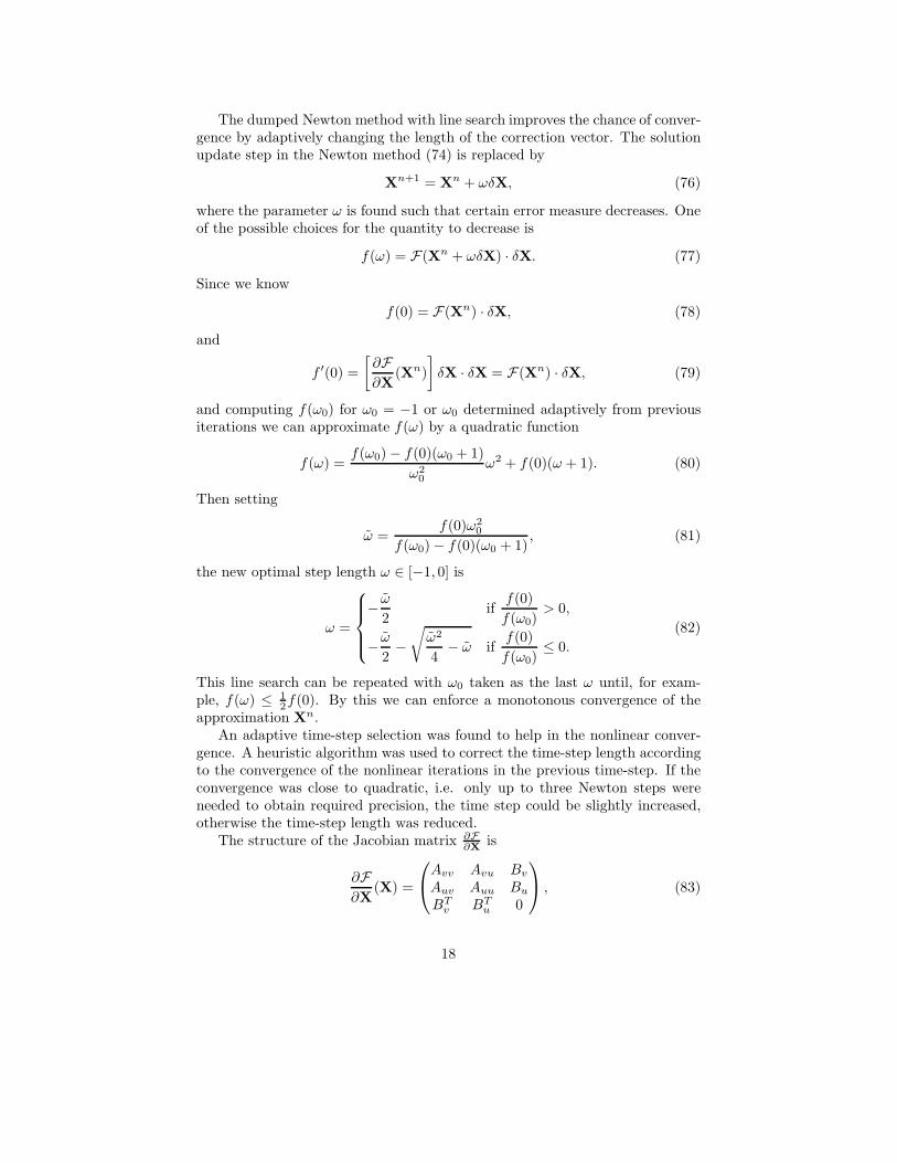
Figure 6: Schematic view of the ventricle and elastic tube geometries.

flow is driven by changing fluid pressure at the inflow part of the boundary whilethe elastic part of the boundary is either fixed or stress free.

The constitutive relations used for the materials are the incompressible New-tonian model (52) for the fluid and the hyper-elastic neo-Hookean material (58)with c2 = 0 for the solid. This choice includes all the main dificulties thenumerical method has to deal with, namely the incompressibility and large de-formations.

5.1 Flow in an ellipsoidal cavity

The motivation for our first test is the left heart ventricle which is approximatelyellipsoidal void surrounded by the heart muscle. In our two-dimensional compu-tations we use an ellipsoidal cavity, see figure 6, with prescribed time-dependentnatural boundary condition at the fluid boundary part Γ1.

p(t) = sin t on Γ1 (118)

The material of the solid wall is modeled by the simple neo-Hookean constitutiverelation (58) with c2 = 0.

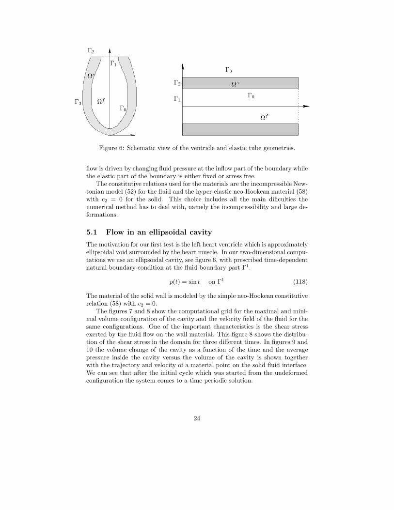
The figures 7 and 8 show the computational grid for the maximal and mini-mal volume configuration of the cavity and the velocity field of the fluid for thesame configurations. One of the important characteristics is the shear stressexerted by the fluid flow on the wall material. This figure 8 shows the distribu-tion of the shear stress in the domain for three different times. In figures 9 and10 the volume change of the cavity as a function of the time and the averagepressure inside the cavity versus the volume of the cavity is shown togetherwith the trajectory and velocity of a material point on the solid fluid interface.We can see that after the initial cycle which was started from the undeformedconfiguration the system comes to a time periodic solution.

24

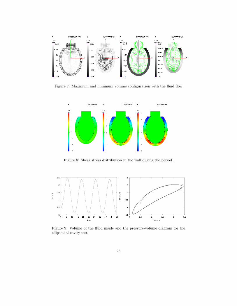
Figure 7: Maximum and minimum volume configuration with the fluid flow

Figure 8: Shear stress distribution in the wall during the period.

Figure 9: Volume of the fluid inside and the pressure-volume diagram for theellipsoidal cavity test.

25

Figure 10: The displacement trajectory and velocity of a point at the fluid solidinterface (inner side of the wall) for the ellipsoidal cavity test

Figure 11: Velocity field during one pulse in channel without an obstacle

5.2 Flow in an elastic channel

The second application is the simulation of a flow in an elastic tube or in our2 dimensional case a flow between elastic plates. The flow is driven by a time-dependent pressure difference between the ends of the channel of the form (118).Such flow is also interesting to investigate in the presence of some constrictionas a stenosis, which is shown in figures 14.

For the flow in the channel without any constriction the time dependence ofthe fluid volume inside the channel is shown together with the pressure volumediagram in the figure and the trajectory and velocity of a material point on thesolid fluid interface in the figures 12 and 13. The velocity field is shown in figure11 at different stages of the pulse.

Finally in figure 14 the velocity field in the fluid and the pressure distributionthroughout the wall is shown for the computation of the flow in a channel with

26

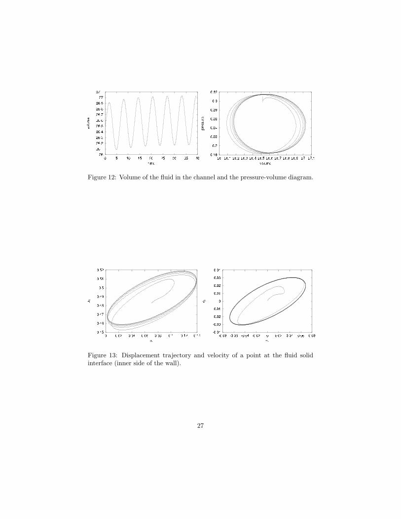
Figure 12: Volume of the fluid in the channel and the pressure-volume diagram.

Figure 13: Displacement trajectory and velocity of a point at the fluid solidinterface (inner side of the wall).

27

Figure 14: Fluid flow and pressure distribution in the wall during one pulse forthe example flow in a channel with constriction

elastic obstruction. In this example the elastic obstruction is modeled by thesame material as the walls of the channel and is fixed to the elastic walls. Bothends of the walls are fixed at the inflow and outflow and the flow is again drivenby a periodic change of the pressure at the left end.

5.3 Illustrative example of perfusion

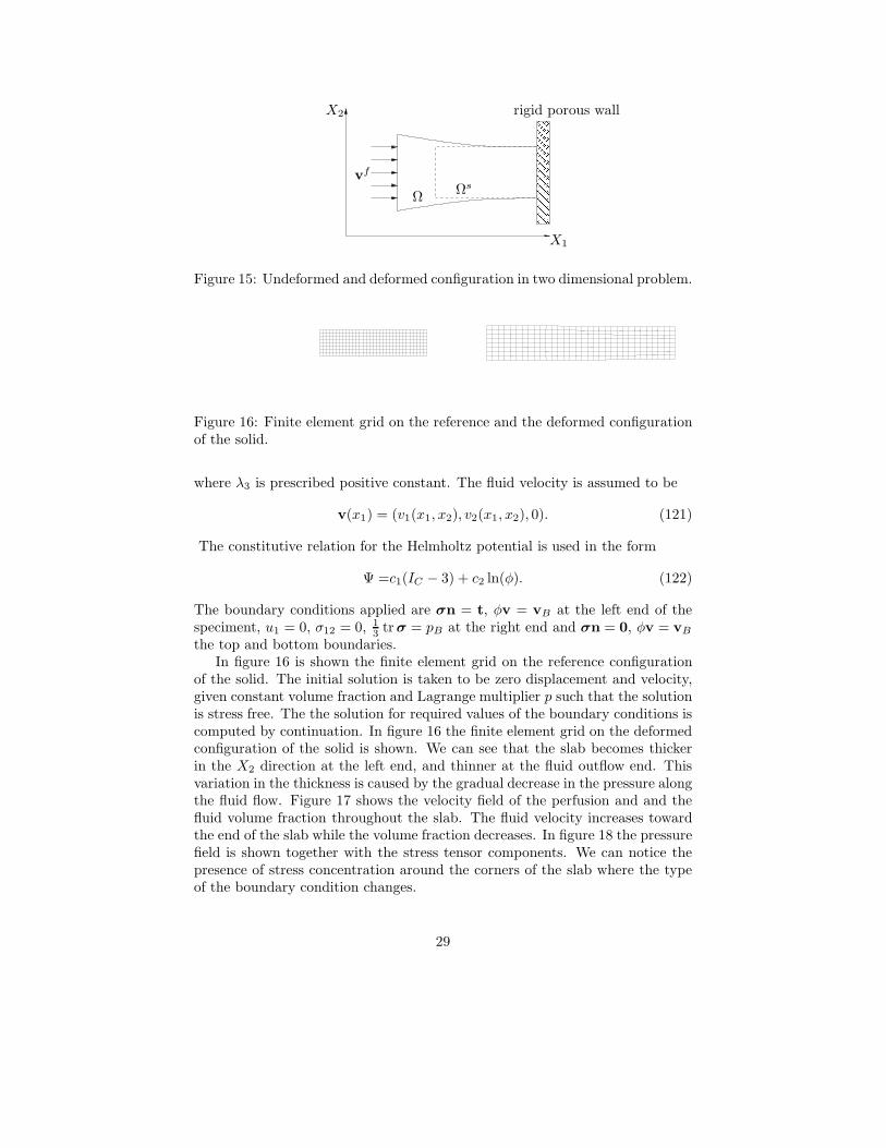
We take two dimensional crossection of the slab along the direction of the per-fusion. Let Ωs = [−L, L]× [−H, H ]× [−L, L] be the reference domain occupiedby the solid. The deformed domain, shown in figure 15, is

Ω = x = X + u(X), ∀X ∈ Ωs. (119)

The deformation is assumed to be of a form

x1 = X1 + u1(X1, X2), x2 = X2 + u2(X1, X2), x3 = λ3X3, (120)

28

rigid porous wall

ΩΩs

vf

X1

X2

Figure 15: Undeformed and deformed configuration in two dimensional problem.

Figure 16: Finite element grid on the reference and the deformed configurationof the solid.

where λ3 is prescribed positive constant. The fluid velocity is assumed to be

v(x1) = (v1(x1, x2), v2(x1, x2), 0). (121)

The constitutive relation for the Helmholtz potential is used in the form

Ψ =c1(IC − 3) + c2 ln(φ). (122)

The boundary conditions applied are σn = t, φv = vB at the left end of thespeciment, u1 = 0, σ12 = 0, 1

3 tr σ = pB at the right end and σn = 0, φv = vB

the top and bottom boundaries.In figure 16 is shown the finite element grid on the reference configuration

of the solid. The initial solution is taken to be zero displacement and velocity,given constant volume fraction and Lagrange multiplier p such that the solutionis stress free. The the solution for required values of the boundary conditions iscomputed by continuation. In figure 16 the finite element grid on the deformedconfiguration of the solid is shown. We can see that the slab becomes thickerin the X2 direction at the left end, and thinner at the fluid outflow end. Thisvariation in the thickness is caused by the gradual decrease in the pressure alongthe fluid flow. Figure 17 shows the velocity field of the perfusion and and thefluid volume fraction throughout the slab. The fluid velocity increases towardthe end of the slab while the volume fraction decreases. In figure 18 the pressurefield is shown together with the stress tensor components. We can notice thepresence of stress concentration around the corners of the slab where the typeof the boundary condition changes.

29

Figure 17: Fluid velocity and the fluid volume fraction.

Figure 18: Isolines of the pressure field and the stress components σ12, σ11 andσ22.

6 Summary and future development

In this paper we present a general formulation of dynamic fluid-structure inter-action problem suitable for applications with finite deformations and laminarflows. While the presented example calculations are simplified to allow initialtesting of the numerical methods the formulation is general to allow immediateextension to more realistic material models. For example in the case of materialanisotropy one can consider

Ψ = c1(IC − 3) + c2(IIC − 3) + c3(|Fa| − 1)2,

with a being the preferred material direction. The term |Fa| represents theextension in the direction a. In Humphrey et al. [1990a,b] a similar materialrelation of the form

Ψ = c1 (exp (b1(IC − 3)) − 1) + c2 (exp (b2(|Fa| − 1)) − 1)

has been proposed to describe a passive behavior of the muscle tissue. Adding toany form of Ψ a term like f(t,x)(|Fa|−1) one can model the active behavior of amaterial and then the system can be coupled with additional models of chemicaland electric activation of the active response of the tissue, see Maurel et al.[1998]. In the same manner the constitutive relation for the fluid can be directlyextended to the power law models used to describe the shear thinning propertyof the blood. Further extension to viscoelastic models and coupling with the

30

mixture based model for soft tissues together with models for chemical andelectric processes involved in biomechanical problems would allow to performrealistic simulation for real applications.

To obtain the solution approximation the discrete systems resulting from thefinite element discretization of the governing equations need to be solved whichrequires sophisticated solvers of nonlinear systems and fast solvers for very largelinear systems. The computational complexity increases tremendously for full3D problems and with more complicated models like visco-elastic materials forthe fluid or solid components. The main advantage of the presented numericalmethod is its accuracy and robustness with respect to the constitutive mod-els. The possible directions of improving the efficiency of the solvers includedevelopment of fast linear solver based on multigrid ideas, spatial and temporaladaptivity and effective use parallel computations.

References

E. S. Almeida and R. L. Spilker. Finite element formulations for hyperelastictransversely isotropic biphasic soft tissues. Comp. Meth. Appl. Mech. Engng.,151:513–538, 1998.

R. Barrett, M. Berry, T. F. Chan, J. Demmel, J. Donato, J. Dongarra, V. Ei-jkhout, R. Pozo, C. Romine, and H. Van der Vorst. Templates for the solution

of linear systems: Building blocks for iterative methods. SIAM, Philadelphia,PA, second edition, 1994.

R. Bramley and X. Wang. SPLIB: A library of iterative methods for sparse linear

systems. Department of Computer Science, Indiana University, Bloomington,IN, 1997. http://www.cs.indiana.edu/ftp/bramley/splib.tar.gz.

K. D. Costa, P. J. Hunter, R. J. M., J. M. Guccione, L. K. Waldman, andA. D. McCulloch. A three-dimensional finite element method for large elasticdeformations of ventricular myocardum: I – Cylindrical and spherical polarcoordinates. Trans. ASME J. Biomech. Eng., 118(4):452–463, 1996a.

K. D. Costa, P. J. Hunter, J. S. Wayne, L. K. Waldman, J. M. Guccione, andA. D. McCulloch. A three-dimensional finite element method for large elasticdeformations of ventricular myocardum: II – Prolate spheroidal coordinates.Trans. ASME J. Biomech. Eng., 118(4):464–472, 1996b.

F. Dai and K. R. Rajagopal. Diffusion of fluids through transversely isotropicsolids. Acta Mechanica, 82:61–98, 1990.

P. S. Donzelli, R. L. Spilker, P. L. Baehmann, Q. Niu, and M. S. Shephard.Automated adaptive analysis of the biphasic equations for soft tissue me-chanics using a posteriori error indicators. Int. J. Numer. Meth. Engng., 34(3):1015–1033, 1992.

31

C. Farhat, M. Lesoinne, and N. Maman. Mixed explicit/implicit time integra-tion of coupled aeroelastic problems: three-field formulation, geometric con-servation and distributed solution. Int. J. Numer. Methods Fluids, 21(10):807–835, 1995. Finite element methods in large-scale computational fluiddynamics (Tokyo, 1994).

Y. C. Fung. Biomechanics: Mechanical properties of living tissues. Springer-Verlag, New York, NY, 2nd edition, 1993.

M. E. Gurtin. Topics in Finite Elasticity. SIAM, Philadelphia, PA, 1981.

P. Haupt. Continuum Mechanics and Theory of Materials. Springer, Berlin,2000.

M. Heil. Stokes flow in collapsible tubes: Computation and experiment. J. Fluid

Mech., 353:285–312, 1997.

M. Heil. Stokes flow in an elastic tube - a large-displacement fluid-structureinteraction problem. Int. J. Num. Meth. Fluids, 28(2):243–265, 1998.

J. D. Humphrey, R. K. Strumpf, and F. C. P. Yin. Determination of a constitu-tive relation for passive myocardium: I. A new functional form. J. Biomech.

Engng., 112(3):333–339, 1990a.

J. D. Humphrey, R. K. Strumpf, and F. C. P. Yin. Determination of a con-stitutive relation for passive myocardium: II. Parameter estimation. J. of

Biomech. Engng., 112(3):340–346, 1990b.

B. Koobus and C. Farhat. Second-order time-accurate and geometrically con-servative implicit schemes for flow computations on unstructured dynamicmeshes. Comput. Methods Appl. Mech. Engrg., 170(1-2):103–129, 1999.

M. K. Kwan, M. W. Lai, and V. C. Mow. A finite deformation theory forcartilage and other soft hydrated connective tissues - I. Equilibrium results.J. Biomech., 23(2):145–155, 1990.

P. Le Tallec and S. Mani. Numerical analysis of a linearised fluid-structureinteraction problem. Num. Math., 87(2):317–354, 2000.

M. E. Levenston, E. H. Frank, and A. J. Grodzinsky. Variationally derived 3-fieldfinite element formulations for quasistatic poroelastic analysis of hydratedbiological tissues. Comp. Meth. Appl. Mech. Engng., 156:231–246, 1998.

F. Marsık. Termodynamika kontinua. Academia, Praha, 1. edition, 1999.

F. Marsık and I. Dvorak. Biothermodynamika. Academia, Praha, 2. edition,1998.

W. Maurel, Y. Wu, N. Magnenat Thalmann, and D. Thalmann. Biomechanical

models for soft tissue simulation. ESPRIT basic research series. Springer-Verlag, Berlin, 1998.

32

M. I. Miga, K. D. Paulsen, F. E. Kennedy, P. J. Hoopes, and D. W. Har-tov, A. Roberts. Modeling surgical loads to account for subsurface tissuedeformation during stereotactic neurosurgery. In IEEE SPIE Proceedings

of Laser-Tissue Interaction IX, Part B: Soft-tissue Modeling, volume 3254,pages 501–511, 1998.

C. W. J. Oomens and D. H. van Campen. A mixture approach to the mechanicsof skin. J. Biomech., 20(9):877–885, 1987.

K. D. Paulsen, M. I. Miga, F. E. Kennedy, P. J. Hoopes, A. Hartov, and D. W.Roberts. A computational model for tracking subsurface tissue deformationduring stereotactic neurosurgery. IEEE Transactions on Biomedical Engi-

neering, 46(2):213–225, 1999.

C. S. Peskin. Numerical analysis of blood flow in the heart. J. Computational

Phys., 25(3):220–252, 1977.

C. S. Peskin. The fluid dynamics of heart valves: experimental, theoretical, andcomputational methods. In Annual review of fluid mechanics, Vol. 14, pages235–259. Annual Reviews, Palo Alto, Calif., 1982.

C. S. Peskin and D. M. McQueen. Modeling prosthetic heart valves for numericalanalysis of blood flow in the heart. J. Comput. Phys., 37(1):113–132, 1980.

C. S. Peskin and D. M. McQueen. A three-dimensional computational methodfor blood flow in the heart. I. Immersed elastic fibers in a viscous incompress-ible fluid. J. Comput. Phys., 81(2):372–405, 1989.

A. Quarteroni. Modeling the cardiovascular system: a mathematical challenge.In B. Engquist and W. Schmid, editors, Mathematics Unlimited - 2001 and

Beyond, pages 961–972. Springer-Verlag, 2001.

A. Quarteroni, M. Tuveri, and A. Veneziani. Computational vascular fluiddynamics: Problems, models and methods. Computing and Visualization in

Science, 2(4):163–197, 2000.

K. R. Rajagopal and L. Tao. Mechanics of mixtures. World Scientific PublishingCo. Inc., River Edge, NJ, 1995.

R. A. Reynolds and J. D. Humphrey. Steady diffusion within a finitely extendedmixture slab. Math. Mech. Solids, 3(2):127–147, 1998.

M. Rumpf. On equilibria in the interaction of fluids and elastic solids. In Theory

of the Navier-Stokes equations, pages 136–158. World Sci. Publishing, RiverEdge, NJ, 1998.

P. A. Sackinger, P. R. Schunk, and R. R. Rao. A Newton-Raphson pseudo-soliddomain mapping technique for free and moving boundary problems: a finiteelement implementation. J. Comput. Phys., 125(1):83–103, 1996.

33

J. J. Shi. Application of theory of a Newtonian fluid and an isotropic non-linear

elastic solid to diffusion problems. PhD thesis, University of Michigan, AnnArbor, 1973.

R. L. Spilker and J. K. Suh. Formulation and evaluation of a finite elementmodel for the biphasic model of hydrated soft tissues. Comp. Struct., Front.

Comp. Mech., 35(4):425–439, 1990.

R. L. Spilker, J. K. Suh, and V. C. Mow. Finite element formulation of the non-linear biphasic model for articular cartilage and hydrated soft tissues includingstrain-dependent permeability. Comput. Meth. Bioeng., 9:81–92, 1988.

J. K. Suh, R. L. Spilker, and M. H. Holmes. Penalty finite element analysis fornon-linear mechanics of biphasic hydrated soft tissue under large deformation.Int. J. Numer. Meth. Engng., 32(7):1411–1439, 1991.

C. Truesdell. A first course in rational continuum mechanics, volume 1. Aca-demic Press Inc., Boston, MA, second edition, 1991.

W. J. Vankan, J. M. Huyghe, J. D. Janssen, and A. Huson. Poroelasticity ofsaturated solids with an application to blood perfusion. Int. J. Engng. Sci.,34(9):1019–1031, 1996.

W. J. Vankan, J. M. Huyghe, J. D. Janssen, and A. Huson. Finite elementanalysis of blood flow through biological tissue. Int. J. Engng. Sci., 35(4):375–385, 1997.

M. E. Vermilyea and R. L. Spilker. Hybrid and mixed-penalty finite elementsfor 3-d analysis of soft hydrated tissue. Int. J. Numer. Meth. Engng., 36(24):4223–4243, 1993.

C. Zoppou, S. I. Barry, and G. N. Mercer. Dynamics of human milk extraction: acomparitive study of breast-feeding and breast pumping. Bull. Math. Biology,59(5):953–973, 1997.

34