entropic risk measures - optimization online ·...

An Analytical Study of Norms and Banach Spaces Induced bythe Entropic Value-at-Risk

Amir Ahmadi-Javid∗ Alois Pichler†

July 28, 2017

Abstract

This paper addresses the Entropic Value-at-Risk (EV@R), a recently introduced coherentrisk measure. It is demonstrated that the norms induced by EV@R induce the same Banachspaces, irrespective of the confidence level. Three spaces, called the primal, dual, and bidualentropic spaces, corresponding with EV@R are fully studied. It is shown that these spacesequipped with the norms induced by EV@R are Banach spaces. The entropic spaces are thenrelated to the Lp spaces, as well as specific Orlicz hearts and Orlicz spaces. This analysisindicates that the primal and bidual entropic spaces can be used as very flexible model spaces,larger than L∞, over which all Lp-based risk measures are well-defined.

The dual EV@R norm and corresponding Hahn–Banach functionals are presented explicitly,which are not explicitly known for the Orlicz and Luxemburg norms that are equivalent to theEV@R norm. The duality relationships among the entropic spaces are investigated. The dualityresults are also used to develop an extended Donsker–Varadhan variational formula, and toexplicitly provide the dual and Kusuoka representations of EV@R, as well as the correspondingmaximizing densities in both representations.

Our results indicate that financial concepts can be successfully used to develop insightfultools for not only the theory of modern risk measurement but also other fields of stochasticanalysis and modeling.

Keywords: Coherent Risk Measures, Dual Representation, Kusuoka Representation,Orlicz Hearts and Spaces, Orlicz and Luxemburg Norms, Lp Spaces, Moment and CumulantGenerating Functions, Donsker–Varadhan Variational Formula, Large Deviations, RelativeEntropy, Kullback-Leibler Divergence

Classification: 90C15, 60B05, 62P05∗Industrial Engineering Department, Amirkabir University of Technology, Tehran, Iran

Contact: [email protected]†Technische Universität Chemnitz, Fakultät für Mathematik, Chemnitz, Germany

Contact: [email protected], https://www.tu-chemnitz.de/mathematik/fima/

1

mailto:[email protected]

mailto:[email protected]

https://www.tu-chemnitz.de/mathematik/fima/

1 Introduction

The literature of risk measures has been extensively developed over the past two decades. Abreakthrough was achieved when the seminal paper Artzner et al. (1999) used an axiomatic approachto define coherent risk measures.

We follow this axiomatic setting and consider a vector space S of R-valued random variables ona reference probability space (Ω, F , P). The set S is called the model space, which is used in thispaper to represent a set of random losses. A risk measure ρ : S → R with R := R ∪ −∞,+∞ iscalled coherent if it satisfies the following four properties:

(P1) Translation invariance: ρ (Y + c) = ρ (Y ) + c for any Y ∈ S and c ∈ R(P2) Subadditivity: ρ (Y1 + Y2) ≤ ρ(Y1) + ρ(Y2) for all Y1, Y2 ∈ S(P3) Monotonicity: If Y1, Y2 ∈ S and Y1 ≤ Y2, then ρ(Y1) ≤ ρ(Y2)(P4) Positive homogeneity: ρ(λY ) = λρ(Y ) for all Y ∈ S and λ > 0

where the convention (+∞) + (−∞) = (−∞) + (+∞) = +∞ is considered. The above settingis usually used in the operations research and insurance literature, while in the finance context,which mostly deals with monetary gains instead of losses, a functional ϕ(·) is called coherent ifρ(Y ) = ϕ(−Y ) satisfies the above four properties.

This paper addresses the Entropic Value-at-Risk (EV@R), a coherent risk measure introduced inAhmadi-Javid (2011) and Ahmadi-Javid (2012a) (see Definition 2.1, and Remarks 2.7 and 4.11 forfinancial interpretations). This risk measure is the tightest upper bound that one can obtain fromChernoff’s inequality for the Value-at-Risk (V@R). In Ahmadi-Javid (2012a) and Ahmadi-Javid(2012b), it is shown that the dual representation of the EV@R can be given using the relativeentropy (also known as Kullback-Leibler divergence) for bounded random variables and thoserandom variables whose moment generating functions exist everywhere, respectively. The Kusuokarepresentation of the EV@R was recently obtained by Delbaen (2018) for bounded random variables.

Ahmadi-Javid (2011) and Ahmadi-Javid (2012a) also extended the EV@R to the class ofϕ-entropic risk measures (see (55)) by replacing the relative entropy in its dual representation withgeneralized entropies (also known as ϕ-divergences). This large class of risk measures includesthe classical Average Value-at-Risk (AV@R, also known as Conditional Value-at-Risk or expectedshortfall). ϕ-entropic risk measures were examined further by Ahmadi-Javid (2012c), Breuer andCsiszár (2013), Breuer and Csiszár (2016), and Shapiro (2017) in developing various decision-making preferences with ambiguity aversion, measuring distribution model risks, and investigatingdistributionally robust counterparts.

There is a close relationship between norms and coherent risk measures defined on the samemodel space. Indeed, a coherent risk measure ρ can be used to define an order-preserving semi-normon the model space S by

‖Y ‖ρ := ρ (|Y |) ,

whenever ρ is finite over S (see Pichler (2014); Pichler (2017) elaborate the reverse statement, aswell as comparisons with other risk measures and norms).

2

This paper starts by investigating the norm induced by the EV@R, called the EV@R norm. TheEV@R norms at the confidence levels α = 0 and α = 1 are identical to the L1 and L∞ norms,respectively. The EV@R norms at different confidence levels 0 < α < 1 are proven to be equivalentto each other, but they do not generate the Lp norms; the Lp norms are bounded by the EV@R normwhile the converse does not hold true. The largest model space contained in the domain of EV@R istherefore strictly larger than L∞, but smaller than every Lp space for 1 ≤ p < ∞ (see Kaina andRüschendorf (2009) for a study of risk measures on Lp spaces).

One should recall that the natural topology defined on⋂

p≥1 Lp, i.e., the smallest topology whichcontains each relative norm topology, cannot be defined by any norm (Arens (1946) and Bell (1977)).Therefore, instead of L∞, one can equip the largest model space corresponding to EV@R with thenorm induced by EV@R and include unbounded random variables in consideration. The new spaceis smaller than every Lp space, but includes all bounded random variables and those unboundedrandom variables whose moment generating functions exist around zero, such as those with normalor exponential distributions. This model space is sufficiently rich for most situations in practice.

The paper presents explicit expressions for the dual EV@R norm and corresponding Hahn–Banach functionals. This is an important achievement because there are no explicit formulas for thedual norm and Hahn–Banach functionals associated with the Orlicz and Luxemburg norms that areequivalent to the EV@R norm.

As side advantages of the duality analysis, we explicitly derive the dual and Kusuoka representa-tions of EV@R, as well as their corresponding maximizing densities, for random variables whosemoment generating functions are finite only around zero. Moreover, we prove an extended versionof the Donsker–Varadhan variational formula and its dual.

It is shown that the EV@R norm, or its dual norm, is indeed equivalent to the Orlicz (orLuxemburg) norm on the associated Orlicz space. Thus, for the entropic spaces one has the generaltopological results that were developed and intensively studied for risk measures on Orlicz heartsand Orlicz spaces in the papers Biagini and Frittelli (2008), Cheridito and Li (2008), Cheriditoand Li (2009), Svindland (2009), and Kupper and Svindland (2011); and more recently in Kieseland Rüschendorf (2014), Farkas et al. (2015), and Delbaen and Owari (2016). The relation toOrlicz spaces further leads to results on risk measures based on quantiles, as addressed in Belliniand Rosazza Gianin (2012) and Bellini, Klar, et al. (2014). However, despite this equivalence tothe Orlicz and Luxamburg norms, the EV@R norm and its dual norm seem favoured in practice,because they are both computationally tractable and their corresponding Hahn–Banach functionalsare available explicitly.

Outline of the paper. Section 2 first introduces the EV@R, entropic spaces, and the associatednorms; and then provides some basic results. Section 3 compares the entropic spaces with otherspaces, particularly to the Lp and Orlicz spaces. Section 4 elaborates duality relations, and providesthe dual norm and Hahn–Banach functionals explicitly. Section 5 concludes the paper by providinga summary and an outlook.

3

2 Entropic Value-at-Risk and entropic spaces

Throughout this paper, we consider the probability space (Ω, F , P). To introduce the EntropicValue-at-Risk for anR-valued random variableY ∈ L0(Ω, F , P), we consider the moment-generatingfunction mY (t) := E etY (cf. Laplace transform).

Definition 2.1 (Ahmadi-Javid (2011)). For an R-valued random variable Y ∈ L0(Ω, F , P) withfinite mY (t0) for some t0 > 0, the Entropic Value-at-Risk (EV@R) at confidence level α ∈ [0, 1] (orrisk level 1 − α) is given by

EV@Rα(Y ) := inft>0

1t

log1

1 − αmY (t) (1)

for α ∈ [0, 1), and is given byEV@R1(Y ) := ess sup(Y ) (2)

for α = 1. Further, the vector spaces

E :=Y ∈ L0 : E et |Y | < ∞ for all t > 0

(3)

E∗ :=Y ∈ L0 : E |Y | log+ |Y | < ∞

1

andE∗∗ :=

Y ∈ L0 : E et |Y | < ∞ for some t > 0

are called the primal, dual, and bidual entropic spaces, respectively.

Remark 2.2 (Entropic spaces). The names chosen here for the spaces E, E∗, and E∗∗ are used tosimplify working with these spaces. Moreover, these names clearly reveal the duality relationshipsamong these spaces, that is, E∗ and E∗∗ are the norm dual and bidual spaces of E (see Section 4).The entropic spaces are also equivalent to specific Orlicz hearts and spaces (see Section 3.2). Somereferences denote the spaces E∗ and E∗∗ by L log L and Lexp, which are related to the Zygmundand Lorentz spaces (see e.g., Section 4.6 of Bennett and Sharpley (1988), and Section 6.7 of Castilloand Rafeiro (2016)).

Remark 2.3 (Relation to insurance). EV@R generalizes the exponential premium principle, which isdefined as

Y 7→1t

logE etY (4)

for t > 0 fixed, see Kaas et al. (2008). The parameter t in (4) is also called the risk aversion parameter.Then, the objective function in (1) can be viewed as a homogenization of an affine perturbation ofthe exponential premium principle, considered in Shapiro et al. (2014, Section 6.3.2).

1log+ z := max0, log z

4

Remark 2.4. The entropic spaces E and E∗∗ are defined in a related way. Distinguishing these twospaces turns out to be fundamental and essential in what follows. For example, it is possible toapproximate random variables Y ∈ E by simple functions, while random variables Y ∈ E∗∗ \ Ecannot (see Section 3 below).

Remark 2.5. EV@R is well-defined on the following domain

E ′ :=Y ∈ L0 : E etY < ∞ for some t > 0

,

and the entropic spaces E and E∗∗ are vector spaces contained in E ′.The set E ′, however, is not a vector space, but it is a convex cone in L0. To see this, consider, for

example, Y := −X where X follows the log-normal distribution. Recall that the moment generatingfunction of the log-normal distribution is finite only on the negative half-axis, so Y belongs to E ′,while neither is Y in E nor in E∗∗.

Remark 2.6 (Cumulant-generating function). The logarithm of the moment-generating function,

KY (t) := logE etY,

is also called the cumulant-generating function of the random variable Y in probability theory (andthe coefficients κ j in the Taylor series expansion KY (t) =

∑j=1 κ j

t j

j! are called cumulants). Hence,EV@R can be rewritten as

EV@Rα(Y ) = inft>0

1t

(KY (t) + log

11 − α

).

One should note that both mY (t) and KY (t) are convex inY for any fixed t, and infinitely differentiableand convex in t for any fixed Y if they are finite.

Remark 2.7 (Lower and upper bounds). We have the following bounds for the EV@R:

EY ≤ EV@Rα(Y ) ≤ ess supY . (5)

The right inequality follows from monotonicity of EV@R. To prove the left one, note that log(·) is aconcave function, and it follows from Jensen’s inequality that

1t

log1

1 − αE etY ≥

1t

log1

1 − α+

1tE log etY ≥ EY,

and henceEY ≤ EV@Rα(Y )

for all 0 ≤ α ≤ 1. Moreover, the above lower bound can be improved by

AV@Rα(Y ) ≤ EV@Rα(Y ), (6)

where AV@Rα is the Average Value-at-Risk at confidence level α ∈ [0, 1), given by

5

AV@Rα(Y ) := inft∈R

t +

11 − α

Emax (Y − t, 0)=

11 − α

∫ 1

αV@Ru (Y )du (7)

and AV@R1(Y ) := ess sup(Y ) for α = 1. V@Rα stands for the Value-at-Risk (or generalized inversecumulative distribution function) at confidence level α ∈ [0, 1], i.e.,

V@Rα(Y ) := infy : P(Y ≤ y) ≥ α

. (8)

From a financial perspective, the inequality (6) indicates that the user of EV@R is more conservativethan who prefers AV@R to quantify the risk Y . The reason is that EV@Rα(Y ) generally incorporatesall V@Rt (Y ) with 0 ≤ t ≤ 1 (see (54)), while AV@Rα(Y ) only depends on V@Rt (Y ) with α ≤ t ≤ 1(see (7)). Actually, under mild conditions, it can be shown that the additional value

EV@Rα(Y ) − AV@Rα(Y )

tends to zero whenever all V@Rt (Y ) with 0 ≤ t < α tend to −∞, which is the best possible outcomefor a risk position.

Remark 2.8 (The special case α = 0). For α = 0, it holds that EV@R0(Y ) = EY forY ∈ E∗∗. Indeed,we have |ey − 1 − y | ≤

y2

2 e |y | by Taylor’s theorem. It follows from Hölder’s inequality that

| E etY − 1 − t EY | ≤t2

2EY 2et |Y | ≤

t2

2

(EY 4

)1/2 (E e2t |Y |

)1/2(9)

whenever Y ∈ E∗∗ and t is small enough. From this, we conclude that the limit for t → 0 exists in (9),further that E etY = 1 + t · EY + O(t2). Using (5), we conclude that EV@R0(Y ) = EY wheneverY ∈ E∗∗.

Remark 2.9 (Convexification of function in (1)). The objective function in (1) can be rewritten as

z log1

1 − αE e

Yz .

The above function is finite and jointly convex in (z,Y ) ∈ R>0 × E ′. Indeed, it is the perspectivefunction associated with the convex function log 1

1−α E eY . The convexity of the latter followsfrom the convexity of the cumulant-generating function KY (t) in Y . This convexity result is highlyimportant when the EV@R is incorporated into large-scale stochastic optimization problems, suchas portfolio optimization and distributionally robust optimization (Ahmadi-Javid and Fallah-Tafti(2017), and Postek et al. (2016)).

EV@R is given as a nonlinear optimization problem in (1). We first characterize the conditionswhen the optimal value in (1) is attained.

Remark 2.10. As a function of t, the objective function in (1) tends to +∞ as the parameter t tendsto zero, and tends to ess sup(Y ) as t tends to∞. The infimum in (1) is thus either attained at somet∗ ∈ (0,∞) or as t tends to∞.

6

Proposition 2.11 (The optimal parameter in (1) to compute EV@R). The following are equivalentfor Y ∈ E ′:

(i) The infimum in (1) is attained at some optimal parameter t∗ ∈ (0,∞)

(ii) V@Rα(Y ) < ess sup(Y )

(iii) P(Y = ess sup(Y )

)< 1 − α

(iv) EV@Rα(Y ) < ess sup(Y ).

Proof. The infimum in (1) is not attained if an increasing parameter t improves the objective, andthis is the case if and only if

1t

log1

1 − αE etY ≥ ess sup(Y )

for all t > 0. This is equivalent to E et (Y−ess sup(Y )) ≥ 1 − α for all t > 0. As Y − ess sup(Y ) ≤ 0,this holds if and only if P

(Y = ess sup(Y )

)≥ 1 − α. The equivalence of the other conditions are

obvious.

We start by comparing the values of EV@R for different confidence levels α, which is used toshow the equivalence of the norms induced by EV@R at different confidence levels.

Proposition 2.12. For 0 < α ≤ α′ < 1 and Y ∈ E ′ it holds that

EV@Rα(Y ) ≤ EV@Rα′ (Y ). (10)

Conversely, if Y ≥ 0 (i.e., Y is in the nonnegative cone) it holds true that

EV@Rα′ (Y ) ≤log(1 − α′)log(1 − α)

· EV@Rα(Y ). (11)

Proof. The inequality (10) is evident by writing 1t log 1

1−α E etY = 1t log 1

1−α +1t logE etY as

log 11−α ≤ log 1

1−α′ .To accept (11), observe that

1t

log1

1 − α′E etY =

1t

(log

11 − α

)·

log(1 − α′)log(1 − α)

+1t

logE etY .

As Y ≥ 0, it follows that logE etY ≥ 0 whenever t > 0. Hence, as log(1−α′)log(1−α) ≥ 1,

1t

log1

1 − α′E etY ≤

1t·

log(1 − α′)log(1 − α)

log1

1 − α+

1t·

log(1 − α′)log(1 − α)

logE etY

=log(1 − α′)log(1 − α)

·1t

log1

1 − αE etY .

7

By taking the infimum among all t > 0 in the latter inequality, it follows that

EV@Rα′ (Y ) ≤log(1 − α′)log(1 − α)

EV@Rα(Y ),

which is the assertion.

Remark 2.13 (Exclusion of the special cases α = 0 and α = 1). The cases α = 0 and α = 1 areexcluded in the previous proposition. Indeed, for α = 0, EV@R0(Y ) = EY ; while for α = 1,EV@R1(Y ) = ess sup Y . Hence, we do not further consider these special cases in what follows.

It is observed in Pichler (2013) and Kalmes and Pichler (2017) that coherent risk measuresinduce semi-norms on vector spaces contained in their domains. In the sequel, we define the EV@Rnorm for Y ∈ E∗∗ by

‖Y ‖ := EV@Rα(|Y |). (12)

The sets E and E∗∗ do not depend on the confidence level, and further, by Proposition 2.12 thenorms (12) are equivalent for different confidence levels 0 < α < 1. For this reason, we do notexplicitly indicate the confidence level α in the notation of the norm ‖ · ‖ = EV@Rα(| · |) in the restof the paper. Recall that for the special cases α = 0 and α = 1, which are excluded in the following,the EV@R norm coincides with the L1 and L∞ norms, respectively.

The next theorem establishes that E (E∗∗, resp.) equipped with the EV@R norm ‖ · ‖ is a Banachspace. This immediately implies that E∗ equipped with the dual EV@R norm ‖ · ‖∗ is a Banachspace.

Theorem 2.14. For 0 < α < 1, the pairs

(E, ‖ · ‖) and (E∗∗, ‖ · ‖)

are (different) Banach spaces for the norm ‖ · ‖ = EV@Rα(| · |).

Proof. It is first shown that E and E∗∗ are complete. We start by considering E∗∗ first. To demonstratecompleteness, let Yn be a Cauchy sequence. For ε > 0, one can find n > 0 such that ‖Yn − Ym‖ < ε

whenever m > n, and thus ‖Ym‖ ≤ ‖Yn‖ + ‖Ym − Yn‖ < ‖Yn‖ + ε. Hence, limn→∞ ‖Yn‖ exists, and‖Yn‖ < C for some constant C < ∞. The norms are, therefore, uniformly bounded.

Now recall that ‖Yn‖ = EV@Rα(|Yn |), so we can choose tn > 0 in (1) to have

1tn

log1

1 − αE etn |Yn | < C. (13)

Next, note that E etn |Yn | ≥ 1; hence,

1tn

log1

1 − α≤

1tn

log1

1 − αE etn |Yn | < C.

It follows thattn > t∗ :=

1C

log1

1 − α> 0,

8

by Fatou’s lemma. Finally

1t∗

log1

1 − αE et

∗ |Y−Yn | ≤1t∗

log1

1 − αet∗ε ≤

1t∗

log1

1 − α+ ε = 2ε

due to (15). It follows that EV@R(|Y − Yn |) → 0, and thus E∗∗ is complete and a Banach space.

The proof that E is complete is along the same lines as for completeness of E∗∗ (particularly (14)),except that it is not necessary to find a number t∗ > 0 for which all moments E etY are well defined;by definition, this is the case for Yn ∈ E. This completes the proof.

3 Comparison with normed spaces

This section relates the entropic spaces with the Lp spaces in the first subsection. To further specifythe nature of the entropic spaces, the EV@R norm is related to specific Orlicz and Luxembourgnorms in the subsequent subsection.

3.1 Comparison with Lp spaces

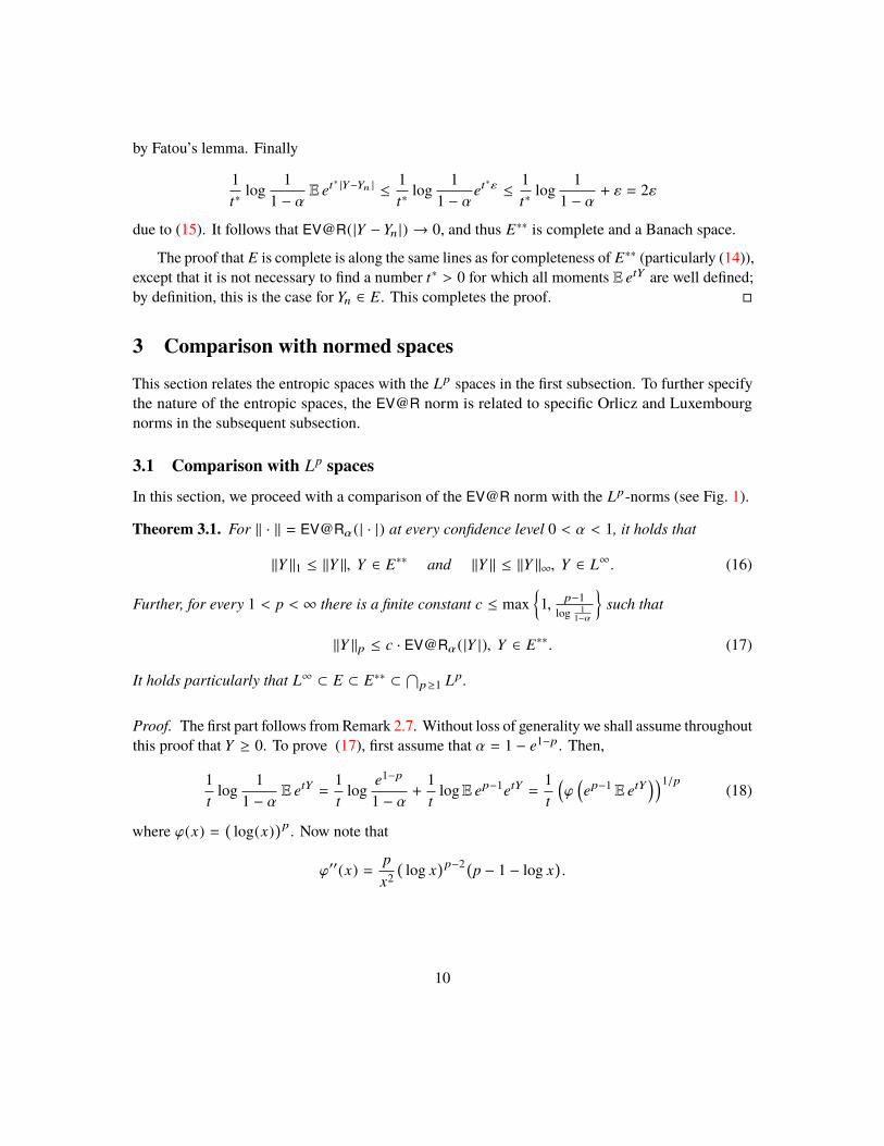
In this section, we proceed with a comparison of the EV@R norm with the Lp-norms (see Fig. 1).

Theorem 3.1. For ‖ · ‖ = EV@Rα( | · |) at every confidence level 0 < α < 1, it holds that

‖Y ‖1 ≤ ‖Y ‖, Y ∈ E∗∗ and ‖Y ‖ ≤ ‖Y ‖∞, Y ∈ L∞. (16)

Further, for every 1 < p < ∞ there is a finite constant c ≤ max1, p−1

log 11−α

such that

‖Y ‖p ≤ c · EV@Rα(|Y |), Y ∈ E∗∗. (17)

It holds particularly that L∞ ⊂ E ⊂ E∗∗ ⊂⋂

p≥1 Lp.

Proof. The first part follows from Remark 2.7. Without loss of generality we shall assume throughoutthis proof that Y ≥ 0. To prove (17), first assume that α = 1 − e1−p. Then,

1t

log1

1 − αE etY =

1t

loge1−p

1 − α+

1t

logE ep−1etY =1t

(ϕ

(ep−1 E etY

))1/p(18)

where ϕ(x) =(log(x)

)p. Now note that

ϕ′′(x) =px2

(log x

)p−2 (p − 1 − log x).

10

L1 E∗ Lp E∗∗ E L∞

Figure 1: Cascading arrangement of the entropic spaces E, E∗, and E∗∗; and their relation to the Lp

spaces, 1 < p < ∞

Hence, the function ϕ(·) is concave (i.e., ϕ′′ ≤ 0) provided that the argument x satisfies x ≥ ep−1;this is the case in (18), as E etY ≥ 1. We apply Jensen’s inequality and obtain

1t

log1

1 − αE etY =

1t

(ϕ

(E ep−1+tY

))1/p≥

1t

(E ϕ

(ep−1+tY

))1/p(19)

=1t

(E(p − 1 + tY )p

)1/p≥

1t

(E(t Y )p

)1/p= ‖Y ‖p,

as t Y ≥ 0. Taking the infimum in (19) among all t > 0 reveals that

‖Y ‖p ≤ EV@R1−e1−p (|Y |).

The assertion follows finally from Proposition 2.12.

Theorem 3.2. L∞ and simple functions are dense in E, but not dense in E∗∗ for the norm‖ · ‖ = EV@Rα(| · |) at any 0 < α < 1.

Remark 3.3. Note that simple functions and L∞ are of course dense whenever α = 0, as they aredense in L1.

Proof. Let Y follow the exponential distribution, i.e., P(e−Y ≤ u

)= u for u > 0. The moment

generating function of this distribution is finite only for t < 1,

E etY =1

1 − t,

which shows that Y ∈ E∗∗ \ E. Further, note that for Yn := minY, n

E et |Y−Yn | ≥ 1,

11

and hence for 0 < α < 1 and t < 1

1t

log1

1 − αE et |Y−Yn | ≥

1t

log1

1 − α≥ log

11 − α

> 0.

Now if Sn is any step function with Sn ≤ n, then |Y − Sn | ≥ |Y − Yn |; and the result follows frommonotonicity.

To accept that simple functions (and consequently L∞) are dense in E, let Y ∈ E be fixed. ByHölder’s inequality,

E etY1Y≥n =P(Y ≤ n

)+ E1Y≥netY

≤1 +(E12

Y≥n

)1/2 (E e2tY

)1/2

=1 + P(Y ≥ n

)1/2(E e2tY

)1/2.

Recall the following extended version of Markov’s inequality,

P(Y ≥ n) ≤E ϕ(Y )ϕ(n)

, (20)

where ϕ(·) is an increasing function and ϕ(n) > 0. We choose ϕ(y) := exp(2ty) in (20), and itfollows that

E etY1Y≥n ≤ 1 +(E e2tY

e2tn

)1/2

·(E e2tY

)1/2= 1 +

E e2tY

etn.

Consequently,

EV@Rα(Y1Y≥n

)≤

1t

log1

1 − α

(1 +E e2tY

etn

)≤

1t

log2

1 − α, (21)

provided that n is sufficiently large. As Y ∈ E, the moment generating function exists for all t > 0.Hence, the latter equation is valid for every t > 0, and it follows that

0 ≤ EV@Rα(Y − Yn) ≤ EV@Rα(Y1Y≥n

) n→∞−−−−→ 0

by monotonicity, where Yn = minY, n.Finally, note that Yn is bounded, and thus it can be approximated sufficiently close by simple

functions (step functions). This completes the proof.

Remark 3.4. We want to point out that all moments of Y exist whenever Y ∈ E, and thus

Y ∈ E =⇒ Y ∈ Lp

for all 1 ≤ p < ∞. However, E is not closed in Lp, and a converse relation to Theorem 3.1 does nothold true on E. More specifically, there is no finite constant c < ∞ for which EV@Rα(|Y |) ≤ c ‖Y ‖pholds true for every Y ∈ E (except p = ∞).

12

We provide an explicit counterexample: consider the random variables Yn with P(Yn = n) = 1/np

and P(Yn = 0) = 1 − 1/np . Then, ‖Yn‖p = 1 and

1t

log1

1 − αE etYn =

1t

log1

1 − α

(1 −

1np+

1np

etn). (22)

Now note that

(22) ≥1t

log1

1 − α(23)

(22) ≥1t

logetn

(1 − α)np= n +

1t

log1

1 − α−

p log nt

. (24)

The function in (23) is decreasing in t, while the function in (24) is increasing for n ≥(

11−α

)1/p.

We choose t = p log nn in (23) and (24), and it follows that EV@Rα(Yn) ≥ n

p log n log 11−α from which

the assertion is immediate.

3.2 Relation to Orlicz spaces

In this section, we demonstrate that the entropic spaces are equivalent to some Orlicz hearts andOrlicz spaces. LetΦ andΨ be coercive convex functions withΦ(0) = Ψ(0) = 0, which are conjugatefunctions to each other. These functions are called a pair of complementary Young functions in thecontext of Orlicz spaces, and they satisfy

y z ≤ Φ(y) + Ψ(z).

Definition 3.5. For a pair Φ and Ψ of complementary Young functions, consider the vector spaces

LΦ := Y ∈ L0 : EΦ(t |Y |) < ∞ for some t > 0

LΦ∗ := Y ∈ L0 : EΦ(t |Y |) < ∞ for all t > 0,

and define the norms‖Y ‖Φ := sup

EΨ( |Z |)≤1EY Z (25)

‖Y ‖(Φ) := inf

k > 0 : EΦ(|Y |k

)≤ 1

. (26)

The norms ‖ · ‖Φ and ‖ · ‖(Φ) are called the Orlicz norm and Luxemburg norm, respectively. Thespaces LΦ and LΦ∗ are called the Orlicz space and Orlicz heart, respectively. In an analogous way,we define LΨ and LΨ∗ , as well as the norms ‖ · ‖Ψ and ‖ · ‖(Ψ).

13

Remark 3.6. The Orlicz norm ‖ · ‖Φ and the Luxemburg norm ‖ · ‖(Φ) are equivalent,

‖Y ‖(Φ) ≤ ‖Y ‖Φ ≤ 2 ‖Y ‖(Φ),

over LΦ (Pick et al. (2012, Theorem 4.8.5)). Hence, we present our results only for the Orlicz normin the following.

In the rest of this paper, we consider the pair

Φ(y) :=

y if y ≤ 1,ey−1 if y ≥ 1

and Ψ(z) :=

0 if z ≤ 1,z log z if z ≥ 1

(27)

of complementary Young functions. It is clear that Φ(y) and ey − 1 are equivalent, in the sense thatthey generate the same Orlicz hearts and spaces.

We have the following relations among the entropic spaces, and the Orlicz hearts and spacescorresponding with Young function Φ(·) given in (27).

Theorem 3.7. It holds that E = LΦ∗ , E∗ = LΨ∗ = LΨ, and E∗∗ = LΦ. Indeed, for 0 < α < 1, thenorms

‖ · ‖ = EV@Rα( | · |) and ‖ · ‖Φ

are equivalent on E∗∗, where Φ is the Young function (27). Particularly, it holds that

‖Y ‖ ≤ c · ‖Y ‖Φ for all Y ∈ E∗∗

for some c ≤ maxe, log 1

1−α

.

Proof. By employing the inequality log y ≤ y − 1 and the elementary inequality

log1

1 − α− 1 + ey ≤ c ·

(1 + Φ(y)

),

which is valid for c = maxe, log 1

1−α

, it follows that

log1

1 − αE et |Y | = log

11 − α

+ logE et |Y | ≤ log1

1 − α− 1 + E et |Y | ≤ c

(1 + EΦ(t |Y |)

),

and henceEV@Rα( |Y |) ≤ c · inf

t>0

1t(1 + EΦ(t |Y |)

). (28)

By Krasnosel’skii and Rutickii (1961, Theorem 10.5) (see also Pick et al. (2012, Remark 4.8.9 (i))),the Orlicz norm has the equivalent expression

‖Y ‖Φ = inft>0

1t(1 + EΦ(t |Y |)

).

14

Therefore, the assertionEV@Rα(Y ) ≤ c · ‖Y ‖Φ for all Y ∈ LΦ (29)

follows from (28). Note that we have particularly proved that Y ∈ LΦ =⇒ Y ∈ E∗∗, i.e., LΦ ⊂ E∗∗.To prove the converse inequality, let Y ∈ E∗∗. Then, by Definition 2.1, there is a number t∗ > 0

such that E etY < ∞ is finite whenever t ≤ t∗. Hence, the Luxemburg norm ‖Y ‖(Φ), given in (26),which is equivalent to the Orlicz norm on LΦ, is also finite because of Φ(x) ≤ 1

e ex . We can, thus,conclude that ‖Y ‖Φ < ∞, i.e., Y ∈ LΦ.

Now consider the identity map

i :(LΦ, ‖ · ‖Φ

)→

(E∗∗, EV@Rα(| · |)

),

which is bounded (‖i‖ ≤ c by (29)). By the above reasoning, i is bijective; and because(E∗∗, EV@Rα(| · |) is a Banach space by Theorem 2.14, it follows from the bounded inversetheorem (open mapping theorem, Rudin (1973, Corollary 2.12)) that the inverse i−1 is continuous aswell, i.e., there is a constant c′ < ∞ such that

‖Y ‖Φ ≤ c′ · EV@Rα(|Y |) for all Y ∈ E∗∗.

Finally note that the function Ψ(·) in Eq. (27) satisfies the ∆2-condition, i.e., Ψ(2x) ≤ k Ψ(x) forevery k > 2 whenever x is large enough. Then, it follows from Pick et al. (2012, Proposition 4.12.3)that LΨ∗ = LΨ, from which the remaining statement is immediate. This completes the proof.

4 Duality

This section first establishes the duality relations of the entropic spaces. In the second part, we providean explicit expression for the EV@R dual norm. To complete the dual description, we explicitlygive the Hahn–Banach functionals, where the Hahn–Banach functional for a norm is an optimalfunctional for the optimization problem corresponding to the dual norm. The last two subsectionsprovide the dual and Kusuoka representations of the EV@R, as well as explicit expressions foroptimal densities in both representations. A new version of the classical Donsker-Varadhan formula,and its dual formula, is also presented.

4.1 Duality of entropic spaces

Theorem 3.7 above makes a series of results developed for Orlicz spaces available for the Banachspaces

(E, ‖ · ‖

), its dual

(E, ‖ · ‖

)∗, and (E∗∗, ‖ · ‖

). We derive the following relations for these

Banach spaces. They reveal that E∗ and E∗∗ are the norm dual and bidual spaces of E.

Theorem 4.1. For ‖ · ‖ = EV@Rα(| · |) at every 0 < α < 1 and the pair of complementary Youngfunctions (27), it holds that

(i)(E, ‖ · ‖

)

(LΦ∗ , ‖ · ‖Φ

)15

(ii)(E∗, ‖ · ‖∗

)

(LΨ∗ , ‖ · ‖Ψ

)

(LΨ, ‖ · ‖Ψ

)(iii)

(E∗∗, ‖ · ‖

)

(LΦ, ‖ · ‖Φ

).

Further, the duality relations

(iv)(E, ‖ · ‖

)∗ (E∗, ‖ · ‖∗

)

(LΨ, ‖ · ‖Ψ

)(v)

(E, ‖ · ‖

)∗∗ (LΨ, ‖ · ‖Ψ

)∗ (LΦ, ‖ · ‖Φ

)

(E∗∗, ‖ · ‖

)hold true (here, denotes the continuous homomorphism and the superscript ∗ the dual space).

Proof. By employing Pick et al. (2012, Theorem 4.13.6), we deduce that(LΦ∗ , ‖ · ‖Φ

)∗

(LΨ, ‖ · ‖Ψ

). (30)

It is evident that E = LΨ∗ by the definition of the spaces, and the equivalence of the norms has alreadybeen established in Theorem 3.7 in a broader context. Thus, (i) and (iv) follow from (30). Moreover,(ii) and (iii) follow from Theorem 3.7 by noting (30).

As for (v), we recall that Ψ(·) in Eq. (27) satisfies the ∆2-condition. Then, it follows from Picket al. (2012, Proposition 4.12.3) that LΨ∗ = LΨ, and further from Pick et al. (2012, Theorem 4.13.6),that the dual space of LΨ is LΦ, i.e.,(

LΨ, ‖ · ‖Ψ)∗

(LΦ, ‖ · ‖Φ

)

(E∗∗, EV@Rα(| · |)

).

Hence, we get (v) by employing (iii) and (i). This completes the proof.

Remark 4.2. One should note thatΦ does not satisfy the ∆2-condition, and hence the space (E, ‖ · ‖)is not reflexive. This follows as well from E∗∗ % E. Moreover, by (iii) in Theorem 4.1, the normdual of E∗∗ can be determined using the results available in the literature of Orlicz spaces (see e.g.,Section 3 of Rao (1968) and Section 2.2 of Biagini and Frittelli (2008)).

Remark 4.3. The duality relations in Theorem 4.1 are specified in the above-mentioned referencesas well. One should note that the following natural mapping (the inner product on LΦ × LΨ):

〈Y, Z〉 7→ EY Z

is the bilinear form considered to study duality results in this section, such as dual norms. Indeed,for each Z in the dual space LΨ, the functional 〈·, Z〉 is the associated continuous linear functionalon the primal space LΦ.

16

4.2 Explicit expression of dual norm

The dual norms corresponding to the Orlicz and Luxemburg norms associated with Young functionsin (27) cannot probably be derived explicitly. To see this, for example, the dual norm ‖ · ‖∗

Φis defined

by‖Z ‖∗Φ = sup

‖Y ‖Φ≤1EY Z,

where ‖ · ‖Φ is given by the rather involved expression (25); recall that the latter is a supremum overa continuum of random variables.

However, for the EV@R, which is equivalent to the above mentioned norms by Theorem 3.7, thefollowing theorem makes a simple explicit expression for the dual norm

‖Z ‖∗ := supEV@Rα ( |Y |)≤1

EY Z

available, which is a supremum over a single parameter. Indeed, the norms ‖ · ‖∗, ‖ · ‖∗Φ, and ‖ · ‖Ψ

(‖ · ‖∗(Φ), and ‖ · ‖(Ψ)) are notably equivalent by Theorem 4.1.

Theorem 4.4 (EV@R dual norm). For 0 < α < 1 and Z ∈ E∗ (i.e., Z ∈ LΨ), we have the explicitexpression

‖Z ‖∗ = supc>0

E |Z | log(|Z |c ∨ 1

)log 1

1−α E(|Z |c ∨ 1

) (31)

for the dual norm ‖ · ‖∗ on E∗, where x ∨ y = maxx, y.

Proof. Without loss of generality, we may assume that Z ≥ 0. Then, it holds that

‖Z ‖∗ = supY,0

EY ZEV@R(|Y |)

= supY,0

EY Z

inft>01t logE 1

1−α et |Y |

= supY,0

supt>0

E Yt Z

1t logE 1

1−α e |Y |= sup

Y,0

EY Z

log 11−α E e |Y |

. (32)

Now define Yc := log(Zc ∨ 1

)and observe that Yc ≥ 0 for every c > 0. Hence,

‖Z ‖∗ ≥ supc>0

E Z log(Zc ∨ 1

)log 1

1−α E(Zc ∨ 1

) , (33)

which is the first inequality required to prove (31).To obtain the converse inequality observe that, by (32), λ ≥ ‖Z ‖∗ is equivalent to

EY Z − λ · log1

1 − αE eY ≤ 0 for every Y ≥ 0.

17

To maximize this latter expression with respect to nonnegative Y ≥ 0, consider the Lagrangian

L(Y, µ) := EY Z − λ · log1

1 − αE eY − EY µ,

where µ is the Lagrangian multiplier associated with the constraint Y ≥ 0. The Lagrangian L isdifferentiable, and its directional derivative with respect to Y in direction H ∈ LΦ is

∂

∂YL(Y, µ)H = E Z H − λ ·

11−α E eY H

11−α E eY

− E µH = E(Z − µ) · H −λ

E eYE eY · H . (34)

The derivative vanishes in every direction H , i.e., ∂L∂Y (Y, µ)H = 0, and it follows from (34) that

Z − µ = c · eY a.s., (35)

where c := λE eY

> 0 is a positive constant. By complementary slackness for the optimal Y ≥ 0 andthe associated multiplier µ ≥ 0 one may conclude that

Y > 0⇐⇒ µ = 0⇐⇒ Z = ceY > c,

and hence, by (35),

Y =

log Zc if Y ≥ 0

0 if Y = 0= log

(Zc∨ 1

).

It is thus sufficient to consider Yc in (33) to prove the remaining assertion.

To evaluate the dual norm numerically, we continue by examining the objective function in (31).

Proposition 4.5. The objective function

ϕα(c) :=E |Z | log

(|Z |c ∨ 1

)log 1

1−α E(|Z |c ∨ 1

)in the expression of the dual norm (31) extends continuously to c = 0, and it holds that

limc↓0

ϕα(c) = E |Z |. (36)

Further, the supremum is attained at some c ≥ 0. If Z , 0 is bounded, then the optimal c satisfies0 ≤ c < ‖Z ‖∞.

Remark 4.6. The function ϕα(·) can be continuously extended to [0,∞). ϕα(·) is, however, notnecessarily monotonic, convex, nor concave in general.

18

Proof. First, note that the objective is continuous and ϕα(·) ≥ 0. One may consider the numeratorand denominator separately for c → ∞ to get

ϕα(c) =E |Z | log

(|Z |c ∨ 1

)log 1

1−α E(|Z |c ∨ 1

) c→∞−−−−→

0log 1

1−α= 0.

For the case c → 0 we find that

ϕα(c) =E |Z | log

(|Z |c ∨ 1

)log 1

1−α E(|Z |c ∨ 1

) = log 1c · E |Z | · (1 + o(1))

log 1c + o(1)

c→0−−−→ E |Z |.

Finally, for c ≥ ‖Z ‖∞ the numerator of ϕα is E |Z | log(|Z |c ∨ 1

)= 0, and thus ϕα(c) = 0, from

which the remaining claim of the proposition follows by the continuity of ϕα(·).

4.3 Hahn–Banach functionals

In this section, we describe the Hahn–Banach functionals corresponding to Y ∈ E∗∗ and Z ∈ E∗

explicitly. That is, we identify the random variable Z ∈ E∗ which maximizes the objective functionin the expression

EV@Rα( |Y |) = supZ,0

EY Z‖Z ‖∗

, (37)

and the random vairable Y ∈ E∗∗ maximizing the objective function in the follwing supremum

‖Z ‖∗ = supY,0

E ZYEV@Rα(|Y |)

. (38)

Proposition 4.7. Let Y ∈ E∗∗ and suppose there is an optimal t∗ ∈ (0,∞) for (1) when Y is replacedby |Y |, then

Z := sign(Y ) · et∗ |Y |

maximizes (37), that is, for ‖ · ‖ = EV@Rα(| · |) at any 0 < α < 1,

‖Y ‖ =EY Z‖Z ‖∗

. (39)

Proof. Without loss of generality, we may assume Y ≥ 0. Consider the function ϕ(t) :=1t log 1

1−α E etY . Given t ′ := supt ∈ (0,∞) : mY (t) < +∞, the function ϕ(·) is continuouslydifferentiable on (0, t ′) with derivative

ϕ′(t) := −1t2 log

11 − α

E etY +1t·

11−α EY etY

11−α E etY

.

19

The point t∗ ∈ (0, t ′) attaining the infimum satisfies ϕ′(t∗) = 0, i.e.,

1t∗

log1

1 − αE et

∗Y =EY et

∗Y

E et∗Y, (40)

so we haveEY Z = EV@Rα(Y ) · E Z,

and thus it is enough to demonstrate that ‖Z ‖∗ = E Z for Z = exp(t∗Y ). By (36), it is sufficient toprove

E Z log(Zc ∨ 1

)log 1

1−α E(Zc ∨ 1

) ≤ E Z

for all c > 0, or the stronger statement

E Z log(Z ∨ c) ≤ E Z · log1

1 − αE(Z ∨ c) (41)

for all c ≥ 0. Note that, by (40), c = 0 satisfies the latter equation. To accept (41), it is enough todemonstrate that the left hand side of (41) grows slower than its right hand side with respect toincreasing c. This is certainly correct if the derivatives of (41) with respect to c satisfy the inequality

EZc1Z≤c ≤ E Z ·

E1Z≤c

E Z ∨ c.

The latter relation derives fromE ZE Z ∨ c

=E Z 1Z≤c + E Z 1Z>c E c1Z≤c + E Z 1Z>c

≥E Z 1Z≤c E c1Z≤c

,

which is a consequence of E c1Z≤c ≥ E Z1Z≤c . This completes the proof.

The following proposition addresses and answers the converse question, i.e., given Z , what isthe random variable Y to obtain equality in (38)?

Proposition 4.8. Let c∗ > 0 be optimal in (31) for Z ∈ E∗. Then,

Y := sign(Z ) · log(|Z |c∗∨ 1

)(42)

satisfies the equalityEY Z = ‖Y ‖ · ‖Z ‖∗.

Proof. Without loss of generality, we may again assume that Z ≥ 0. By (31) and the definition of Yin (42) we have that

‖Z ‖∗ =EY Z

log 11−α E eY

,

and henceEY Z ≤ ‖Z ‖∗ · EV@Rα(|Y |) ≤ ‖Z ‖∗ · log

11 − α

E eY = EY Z,

from which we conclude the assertion.

20

4.4 Dual representation and extended Donsker–Varadhan formula

Wederive the dual representation ofEV@R forY ∈ E∗∗ from the characterizations already establishedfor the norms in the previous section. As stated in the introduction, the dual representation given inthe following theorem was already shown for Y ∈ L∞ and Y ∈ E in the literature.

Theorem 4.9 (Dual representation of EV@R). For every 0 < α < 1 and Y ∈ E∗∗, the EV@R hasthe representation

EV@Rα(Y ) = supEY Z : E Z = 1, Z ≥ 0 and E Z log Z ≤ log

11 − α

. (43)

Proof. The proof of Proposition 4.7 can be applied to similarly show that the equation

EV@Rα(Y ) =EY Z‖Z ‖∗

. (44)

holds for some density Z ∈ E∗. This implies the following representation:

EV@Rα(Y ) = supEY Z : E Z = 1, Z ≥ 0 and ‖Z ‖∗ ≤ 1

.

From the representation (31) of the norm and (36) it follows that

E Z log(Zc ∨ 1

)log 1

1−α E(Zc ∨ 1

) ≤ E Z .

By the same reasoning as in the previous proof, we have

E Z log (Z ∨ c) ≤ E Z · log1

1 − αE (Z ∨ c)

for every c ≥ 0. By setting c = 0 and assuming E Z = 1 (which follows from the translationinvariance property (P1)), we obtain

E Z log Z ≤ log1

1 − α.

This concludes the proof.

Remark 4.10. A random variable Z with E Z = 1 and Z ≥ 0 represents a density and

Q(B) := E1BZ

is a measure, which is absolutely continuous with respect to the probability measure P. Therefore,the expression E Z log Z represents the relative entropy of Q with resepct to P (also known asKullback–Leibler divergence of Q from P, denoted by D(Q ‖ P)) (cf. (45)).

21

Remark 4.11 (A financial interpretation). A nice financial interpretation of EV@R(Y ) can be givenbased on the dual representation presented in Theorem 4.9. Namely, EV@R(Y ) is the largestexpected value of Y over all probability measures Q which are absolutely continuous with respect toP and have a Kullback-Leibler divergence D(Q ‖ P) less than some positive value (informally, allmeasures Q within a ball around P defined based on the relative entropy), that is,

EV@Rα(Y ) = supQP

EQ (Y ) : D(Q ‖ P) = EP

(dQdP log dQ

dP

)≤ − log (1 − α)

. (45)

This gives the interpretation of EV@R(Y ) as a model risk quantification when it is compared toEP (Y ) in the presence of model ambiguity, which has been widely studied over the past severaldecades in economics, finance, and statistics (see the seminal papers Ellsberg (1961) and Gilboa andSchmeidler (1989); and also Ahmadi-Javid (2012c), Breuer and Csiszár (2016), Watson and Holmes(2016), and references therein).

We further explicitly describe the maximising Z ∈ E∗ for the dual representation (43) of EV@R.

Proposition 4.12 (The maximizing density of the dual representation of EV@R). Suppose thatY ∈ E∗∗. If V@Rα(Y ) < ess sup(Y ) (or equivalently, P

(Y = ess sup(Y )

)< 1 − α), the supremum

in (43) is attained for

Z∗ :=et∗Y

E et∗Y,

where t∗ > 0 is the optimal parameter for (1). This density satisfies

E Z∗ log Z∗ = log1

1 − α.

If V@Rα(Y ) = ess sup(Y ), or equivalently, P(Y = ess sup(Y )

)≥ 1 − α, the supremum is attained

for

Z∗ =

P(Y = ess sup(Y )

)−1 if Y = ess sup(Y ),0 else.

Proof. From Proposition 2.11, V@Rα(Y ) < ess sup(Y ) if and only if the optimal parameter t∗ for (1)is a finite value in (0,∞). Then, to obtain the equality, consider (40) in the proof of Proposition 4.7,which can be rewritten as

1t∗

log1

1 − αE et

∗Y =EY et

∗Y

E et∗Y= EY Z∗, (46)

and thus EV@Rα(Y ) = EY Z∗.It is further evident that Z∗ ≥ 0, E Z∗ = 1, and it holds that

E Z∗ log Z∗ = Eet∗Y

E et∗Y(t∗Y − logE et

∗Y).

22

By (46) it follows that


1 − αE et

∗Y − logE et∗Y = log

11 − α

.

If V@Rα(Y ) = ess sup(Y ), the remaining assertion follows from EV@Rα(Y ) = ess sup(Y ).

Corollary 4.13 (Donsker–Varadhan variational formula). TheDonsker–Varadhan variational formula

E Z log Z = supEY Z − logE eY : Y ∈ E

(47)

holds true; further, the latter expression is finite only for densities Z ∈ E∗. Conversely, for anyY ∈ E

logE eY = supEY Z − E Z log Z : Z ∈ E∗, E Z = 1, Z ≥ 0

. (48)

Remark 4.14. The equation (47) is an alternative expression for the Kullback-Leibler divergence(see Remark 4.10) based on convex conjugate duality. In the classical Donsker–Varadhan variationalformula (see Lemma 1.4.3 and Appendix C.2 of Dupuis and Ellis (1997)), the supremum is takenover Y ∈ L∞. The formula (47) shows that the optimal value remains intact after extending theoptimization domain to Y ∈ E. The dual formula (48) is also extended for a broader range of randomvariables Y ∈ E, while the old version is given for Y ∈ L∞ (see Proposition 1.4.2 of Dupuis andEllis (1997)). It should be remarked that the latter variational formula plays a key role in weakconvergence approach to large deviations.

Proof. To verify the Donsker–Varadhan variational formula (47), we define the convex and closedset

ζα :=

Z ∈ E∗ : E Z = 1, Z ≥ 0 and E Z log Z ≤ log1

1 − α

(49)

and its support function

Iζα (Z ) :=

0 if Z ∈ ζα,+∞ else.

By the Fenchel–Moreau duality theorem (Shapiro et al. (2014, Theorem 7.5)) and the dualrepresentation of EV@R, we have that

Iζα (Z ) = supY ∈EEY Z − EV@Rα(Y )

= supt>0,Y ∈E

EY Z −1t

log1

1 − αE etY

= supY ∈E, t>0

1t

(EY Z − logE eY − log

11 − α

).

It follows that Z ∈ ζα if and only if

EY Z − logE eY ≤ log1

1 − αfor all Y ∈ E. (50)

The Donsker–Varadhan variational formula follows now by considering all values 0 < α < 1 in (49)and (50). The converse similarly follows by convex conjugate duality.

23

4.5 Kusuoka representation

The EV@R is a law invariant (version independent) coherent risk measure for which a Kusuokarepresentation can be obtained (Kusuoka (2001) and Pflug and Römisch (2007)). We derive theKusuoka representation of EV@R from its dual representation (Theorem 4.9; see also Delbaen(2018)).

Proposition 4.15 (Kusuoka representation). The Kusuoka representation of the EV@R for Y ∈ E∗∗

is

EV@Rα(Y ) = supµ

∫ 1

0AV@Rp (Y )µ(dp), (51)

where the supremum is among all probability measures µ on [0, 1) for which the associated distortionfunction

σµ (p) :=∫ p

0

11 − u

µ(du)

satisfies ∫ 1

0σµ (p) log

(σµ (p)

)dp ≤ log

11 − α

. (52)

The supremum in (51) is attained for the measure µσ∗ associated with the distortion function

σ∗(p) := F−1Z∗ (p) = V@Rp (Z∗), (53)

where Z∗ is the optimal random variable addressed in Proposition 4.12.

Remark 4.16 (Alternative formulation). The Kusuoka representation (51) can be stated alternativelyby

EV@Rα(Y ) = supσ

∫ 1

0σ(u) · V@Ru (Y )du, (54)

where the supremum is taken over the set of distortion functions σ (i.e., σ(·) is a nondecreasingdensity on [0, 1)) satisfying (52) (with σ in lieu of σµ).

Remark 4.17. The formulation (54) of EV@R is the rearranged formulation of the dual representa-tion (43) in Theorem 4.9. Indeed, Y and the optimal Z∗ are comonotone random variables, and thefunctions σ(u) = V@Ru (Z∗) and V@Ru (Y ) represent their nondecreasing rearrangements in (54)(Pflug and Römisch (2007)). The constraint (52) finally explicitly involves the Kullback–Leiblerdistance for the nondecreasing density Z∗.

Proof of Proposition 4.15. The representation is immediate from the dual formula (43) and thegeneral description given in Pflug and Pichler (2014, pp. 100) or Pichler and Shapiro (2015).

To see the optimal measure in (53), when t∗ ∈ (0,∞), observe that


1 − α

24

by the definition of Z∗ and Proposition 4.12, and further that

E Z∗ log Z∗ =∫ 1

0σ∗(u) logσ∗(u)du

by the definition of σ∗ in (53). Define next the measure

µ∗(A) := σ∗(0) · δ0(A) +∫

A

(1 − u)dσ∗(u) (A ⊂ [0, 1) is measurable)

by Riemann–Stieltjes integration on the unit interval.For this measure µ∗ it holds that∫ p

0

11 − u

µ∗(du) = σ∗(0) +∫ p

0

11 − u

(1 − u)dσ∗(u) = σ∗(p),

and σ∗ is therefore feasible for (51). Observe finally that∫ 1

0AV@Rα(Y )µ∗(dα) = σ∗(0) AV@R0(Y ) +

∫ 1

0

11 − α

∫ 1

αF−1Y (u)du (1 − α)dσ∗(α)

=

∫ 1

0σ∗(u)F−1

Y (u)du = E Z∗Y = EV@Rα(Y )

by Riemann–Stieltjes integration by parts. Hence, the assertion follows.

5 Summary and outlook

This paper considers the norm and dual norm induced by Entropic Value-at-Risk (EV@R), whichare proven to be equivalent at different confidence levels 0 < α < 1. The paper also studies therelated vector spaces E, E∗, and E∗∗, which are called the primal, dual, and bidual entropic spaces,respectively. The primal and bidual entropic spaces are model spaces over which the EV@R norm‖ · ‖ := EV@R( | · |) is also well-defined. The spaces E∗ and E∗∗ are the norm dual and bidualspaces of the primal entropic space E; they are all not reflexive. The pairs (E, ‖ · ‖), (E∗, ‖ · ‖∗),and (E∗∗, ‖ · ‖) are Banach spaces.

Moreover, it is shown that E is an Orlicz heart with E∗∗ being its related Orlicz space, onwhich the associated Orlicz norm (Luxemburg norm) is proven to be equivalent to the EV@R norm.Similarly, it is shown that E∗ is an Orlicz heart coinciding with its corresponding Orlicz space, overwhich both the dual EV@R norm and its related Orlicz norm (Luxemburg norm) are equivalent.These observations alert us to the fact that the topological results developed for risk measures overthe Orlicz hearts and spaces can be directly applied to the entropic spaces.

Both primal and bidual entropic spaces are subsets of the intersection of all the Lp spaces,including many unbounded random variables, while both are significantly larger than L∞. ThoughL∞ is dense in E, the space E∗∗ includes unbounded random variables which are not the limit of

25

any sequence of bounded random variables. Therefore, considering that the natural topology on⋂p≥1 Lp is not normable, one can use the larger spaces E and E∗∗ as a model space instead of L∞

when a flexible model space is needed over which all the Lp-based risk measures are well-defined.The formulas of the EV@R dual norm and corresponding Hahn–Banach functionals are explicitly

obtained This highlights the computational and analytical advantages of using EV@R norm andits dual norm in practice when dealing with risk measures over the entropic spaces. One shouldnote that the dual norm and Hahn–Banach functionals are not explicitly known for the Orlicz (orLuxemburg) norm that is equivalent to the EV@R norm. Using the duality results, the dual and theKusuoka representations of EV@R, as well as their corresponding maximizing densities, are derivedexplicitly. In addition, the duality analysis results in an extended version of Donsker–Varadhanvariational formulas and its dual which involve unbounded random variables.

The analysis presented here shows that one can develop powerful analytical tools in probabilitytheory based on risk measures. This promising avenue from modern risk measure theory toprobability theory can be more investigated in future studies. For example, following the idea used inthis paper, one can develop new norms based on the rich class of ϕ-entropic risk measures given by

ERϕ,β (Y ) = sup EY Z : E Z = 1, Z ≥ 0 and E ϕ(Z ) ≤ β (55)

for an increasing convex function ϕ with ϕ(1) = 0 and β ≥ 0. These information-theoretic riskmeasures are coherent, which can be efficiently computed using the primal representation

ERϕ,β (Y ) = infz>0, µ∈R

zµ + z E ϕ∗

(Yz− µ + β

),

where ϕ∗ is the conjugate of ϕ (Theorem 5.1 in Ahmadi-Javid (2012a)). The norm induced by ERϕ,βis conjectured to be equivalent to the Orlicz norm (Luxemburg norm) on the corresponding Orliczspace Lϕ

∗ under mild conditions.

References

Ahmadi-Javid, A. (2011). “An information-theoretic approach to constructing coherent riskmeasures”. In: 2011 IEEE International Symposium on Information Theory Proceedings,pp. 2125–2127.

— (2012a). “Entropic value-at-risk: A new coherent risk measure”. In: Journal of OptimizationTheory and Applications 155.3, pp. 1105–1123.

— (2012b). “Addendum to: Entropic value-at-risk: A new coherent risk measure”. In: Journal ofOptimization Theory and Applications 155.3, pp. 1124–1128.

— (2012c). “Application of information-type divergences to constructing multiple-priors andvariational preferences”. In: 2012 IEEE International Symposium on Information TheoryProceedings, pp. 538–540.

26

Ahmadi-Javid, A. and M. Fallah-Tafti (2017). “Portfolio optimization with entropic value-at-risk”.Optimization Online.

Arens, R. (1946). “The space Lω and convex topological rings”. In: Bulletin of the AmericanMathematical Society 52.10, pp. 931–935.

Artzner, P., F. Delbaen, J.-M. Eber, and D. Heath (1999). “Coherent measures of risk”. In:Mathematical Finance 9.3, pp. 203–228.

Bell, W. C. (1977). “On the normability of the intersection of Lp spaces”. In: Proceedings of theAmerican Mathematical Society 66.2, pp. 299–304.

Bellini, F., B. Klar, A. Müller, and E. Rosazza Gianin (2014). “Generalized quantiles as riskmeasures”. In: Insurance: Mathematics and Economics 54, pp. 41–48.

Bellini, F. and E. Rosazza Gianin (2012). “Haezendonck–Goovaerts risk measures and Orliczquantiles”. In: Insurance: Mathematics and Economics 51.1, pp. 107–114.

Bennett, C. and R. Sharpley (1988). Interpolation of Operators. Academic Press.

Biagini, S. and M. Frittelli (2008). “A unified framework for utility maximization problems: AnOrlicz space approach”. In: Annals of Applied Probability 18.3, pp. 929–966.

Breuer, T. and I. Csiszár (2013). “Information geometry in mathematical finance: Model risk, worstand almost worst scenarios”. In: 2013 IEEE International Symposium on Information TheoryProceedings, pp. 404–408.

Breuer, T. and I. Csiszár (2016). “Measuring distribution model risk”. In:Mathematical Finance26.2, pp. 395–411.

Castillo, R. E. and H. Rafeiro (2016). An Introductory Course in Lebesgue Spaces. CMS books inMathematics. Springer.

Cheridito, P. and T. Li (2008). “Dual characterization of properties of risk measures on Orliczhearts”. In: Mathematics and Financial Economics 2.1, pp. 29–55.

— (2009). “Risk measures on Orlicz hearts”. In: Mathematical Finance 19.2, pp. 189–214.

Delbaen, F. (2018). “Remark on the paper "Entropic value-at-risk: A new coherent risk measure" byAmir Ahmadi-Javid”. In: Risk and Stochastics. Ed. by P. Barrieu. World Scientific, Availableonline at arXiv preprint, arXiv:1504.00640.

Delbaen, F. and K. Owari (2016). “On convex functions on the duals of ∆2-Orlicz spaces”. In: arXivpreprint, arXiv:1611.06218.

Dupuis, P. and R. S. Ellis (1997). A Weak Convergence Approach to the Theory of Large Deviations.Wiley.

Ellsberg, D. (1961). “Risk, ambiguity, and the Savage axioms”. In: The Quarterly Journal ofEconomics 75.4, pp. 643–669.

27

Farkas, W., P. Koch-Medina, and C. Munari (2015). “Measuring risk with multiple eligible assets”.In: Mathematics and Financial Economics 9.1, pp. 3–27.

Gilboa, I. and D. Schmeidler (1989). “Maxmin expected utility with non-unique prior”. In: Journalof Mathematical Economics 18.2, pp. 141–153.

Kaas, R., M. Goovaerts, J. Dhaene, and M. Denuit (2008). Modern Actuarial Risk Theory. 2nd.Springer.

Kaina, M. and L. Rüschendorf (2009). “On convex risk measures on Lp-spaces”. In: MathematicalMethods of Operations Research 69.3, pp. 475–495.

Kalmes, T. and A. Pichler (2017). “On Banach spaces of vector-valued random variables and theirduals motivated by risk measures”. In: Banach Journal of Mathematical Analysis, to appear.

Kiesel, S. and L. Rüschendorf (2014). “Optimal risk allocation for convex risk functionals in generalrisk domains”. In: Statisticas and Risk Modeling 31.3–4, pp. 335–365.

Krasnosel’skii, M. A. and Y. B. Rutickii (1961). Convex Functions and Orlicz Spaces. NoordhoffGroningen.

Kupper, M. and G. Svindland (2011). “Dual reopresentation of monotone convex functions on L0”.In: Proceedings of the American Mathematical Society 139.11, pp. 4073–4086.

Kusuoka, S. (2001). “On law invariant coherent risk measures”. In: Advances in MathematicalEconomics. Ed. by S. Kusuok and T. Maruyama. Vol. 3. Springer, pp. 83–95.

Pflug, G. Ch. and A. Pichler (2014). Multistage Stochastic Optimization. Springer Series inOperations Research and Financial Engineering. Springer.

Pflug, G. Ch. and W. Römisch (2007). Modeling, Measuring and Managing Risk. World Scientific.

Pichler, A. (2013). “The natural Banach space for version independent risk measures”. In: Insurance:Mathematics and Economics 53.2, pp. 405–415.

— (2014). “Insurance pricing under ambiguity”. In: European Actuarial Journal 4.2, pp. 335–364.

— (2017). “A quantitative comparison of risk measures”. In: Annals of Operations Research254.1-2, pp. 251–275.

Pichler, A. and A. Shapiro (2015). “Minimal representations of insurance prices”. In: Insurance:Mathematics and Economics 62, pp. 184–193.

Pick, L., A. Kufner, O. John, and S. Fučík (2012). Function Spaces, 1. De Gruyter Series inNonlinear Analysis and Applications. De Gruyter.

Postek, K., D. den Hertog, and B. Melenberg (2016). “Computationally tractable counterparts ofdistributionally robust constraints on risk measures”. In: SIAM Review 58.4, pp. 603–650.

Rao, M. (1968). “Linear functionals on Orlicz spaces: General theory”. In: Pacific Journal ofMathematics 25.3, pp. 553–585.

28

Rudin, W. (1973). Functional Analysis. McGraw-Hill.

Shapiro, A., D. Dentcheva, and A. Ruszczyński (2014). Lectures on Stochastic Programming. 2ndedn. MOS-SIAM Series on Optimization. Society for Industrial and Applied Mathematics.

Shapiro, A. (2017). “Distributionally robust stochastic programming”. In: SIAM Journal onOptimization, to appear.

Svindland, G. (2009). “Subgradients of law-invariant convex risk measures on L1”. In: Statistics &Decisions 27.2, pp. 169–199.

Vaart, A. W. van der (1998). Asymptotic Statistics. Cambridge University Press.

Watson, J. and C. Holmes (2016). “Approximate models and robust decisions”. In: StatisticalScience 31.4, pp. 465–489.

July 28, 2017, output

29

entropic risk measures - optimization online ·...

Documents