Sensors 2008, 8, 4119-4134; DOI: 10.3390/s8074119

sensors ISSN 1424-8220

www.mdpi.org/sensors Article

A Methodology to Validate the InSAR Derived Displacement Field of the September 7th, 1999 Athens Earthquake Using Terrestrial Surveying. Improvement of the Assessed Deformation Field by Interferometric Stacking Ioannis Kotsis 1, Charalabos Kontoes 2,*, Dimitrios Paradissis 1, Spyros Karamitsos 1, Panagiotis Elias 2 and Ioannis Papoutsis 2

1 Higher Geodesy Laboratory and Dionyssos Satellite Observatory, National Technical University of

Athens, Iroon Polytexneiou 9, 15780, Zografou, Greece; E-Mails: jkotsis@survey.ntua.gr (I.K.);

dempar@central.ntua.gr (D.P.); karamits@central.ntua.gr (S.K.)

2 National Observatory of Athens, Institute of Space Applications and Remote Sensing, Vas. Pavlou

and Metaxa str., 15236, Palaia Penteli, Greece; E-mails: pelias@space.noa.gr (P.E.);

ipapoutsis@space.noa.gr (I.P.)

* Author to whom correspondence should be addressed; E-Mail: kontoes@space.noa.gr (C.K.)

Received: 20 March 2008; in revised form: 19 June 2008 / Accepted: 20 June 2008 /

Published:10 July 2008

Abstract: The primary objective of this paper is the evaluation of the InSAR derived

displacement field caused by the 07/09/1999 Athens earthquake, using as reference an

external data source provided by terrestrial surveying along the Mornos river open

aqueduct. To accomplish this, a processing chain to render comparable the leveling

measurements and the interferometric derived measurements has been developed. The

distinct steps proposed include a solution for reducing the orbital and atmospheric

interferometric fringes and an innovative method to compute the actual InSAR estimated

vertical ground subsidence, for direct comparison with the leveling data. Results indicate

that the modeled deformation derived from a series of stacked interferograms, falls

entirely within the confidence interval assessed for the terrestrial surveying data.

Keywords: Ground subsidence, SAR Interferometry, stacked interferogram, leveling.

OPEN ACCESS

Sensors 2008, 8

4120

1. Introduction

One of the most significant natural disasters to strike Greece in the 20th century was the September

7, 1999, 11h 56m 50s UTC, Mw (moment magnitude) = 5.9 Athens earthquake. It claimed the lives of

143 people, and caused the collapse of several buildings, mainly in the northwest suburbs of the Greek

capital. The approximate location of the earthquake epicenter was 38.10oN, 23.56oE, roughly 20 km

northwest from the center of Athens [1].

The vertical displacement field at the surface level caused by this tectonic event was investigated

with space born Synthetic Aperture Radar Interferometry (InSAR), using ERS-2 data. InSAR

processing showed a significant deformation with the maximum Line Of Sight (LOS) subsidence being

of approximately 6 cm [1]. This observation was used in earthquake modeling and fault location

mapping [2-9] along the middle of the Parnitha mountain. However, the deformation field reported in

[1] could not be verified at that time due to the lack of co-seismic geodetic measurements of adequate

precision. The sole indication was provided by geologists and engineers who visited the area and

confirmed that the damaged structures, at the substructure level, were showing a vertical movement of

the same order of magnitude as the InSAR derived assessments.

The region of maximum deformation coincided with the main shock epicenter. This area was very

close to the Mornos river open aqueduct, used for water supply to Athens. The distance of the aqueduct

pass from the earthquake epicenter was less than 2.5 km. The water supply authority in Athens

awarded an aqueduct-leveling project to the National Technical University of Athens/Higher Geodesy

department (NTUA/HG), which lasted for two months, from March to April 2001. Prior leveling data

along the Mornos aqueduct had been obtained in 1984. No height data were available for the

intermediate time interval 1984-2001; however no major seismic event had taken place in that period.

The two co-seismic sets of leveling data were considered adequate to investigate the vertical

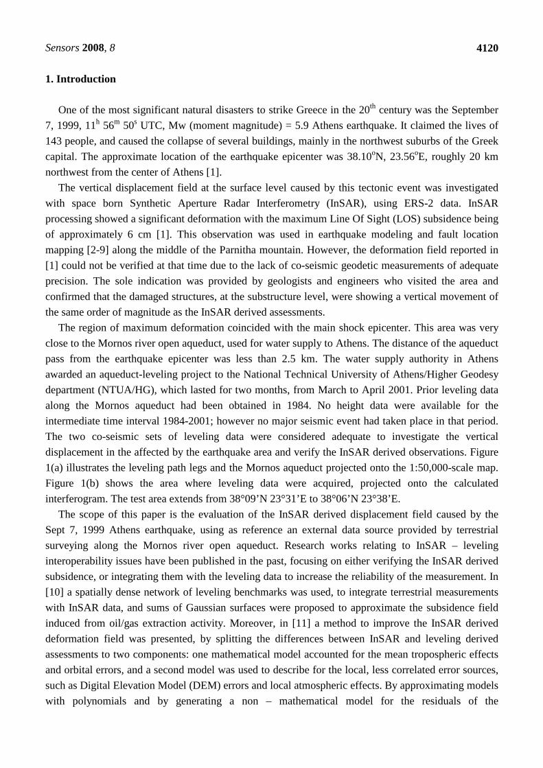
displacement in the affected by the earthquake area and verify the InSAR derived observations. Figure

1(a) illustrates the leveling path legs and the Mornos aqueduct projected onto the 1:50,000-scale map.

Figure 1(b) shows the area where leveling data were acquired, projected onto the calculated

interferogram. The test area extends from 38°09’N 23°31’E to 38°06’N 23°38’E.

The scope of this paper is the evaluation of the InSAR derived displacement field caused by the

Sept 7, 1999 Athens earthquake, using as reference an external data source provided by terrestrial

surveying along the Mornos river open aqueduct. Research works relating to InSAR – leveling

interoperability issues have been published in the past, focusing on either verifying the InSAR derived

subsidence, or integrating them with the leveling data to increase the reliability of the measurement. In

[10] a spatially dense network of leveling benchmarks was used, to integrate terrestrial measurements

with InSAR data, and sums of Gaussian surfaces were proposed to approximate the subsidence field

induced from oil/gas extraction activity. Moreover, in [11] a method to improve the InSAR derived

deformation field was presented, by splitting the differences between InSAR and leveling derived

assessments to two components: one mathematical model accounted for the mean tropospheric effects

and orbital errors, and a second model was used to describe for the local, less correlated error sources,

such as Digital Elevation Model (DEM) errors and local atmospheric effects. By approximating models

with polynomials and by generating a non – mathematical model for the residuals of the

Sensors 2008, 8

4121

approximations, corrections for the InSAR derived deformations were produced for the entire SAR

image. In [12] a study for mine subsidence monitoring using ERS-1/2 and JERS-1/2 was investigated,

combining the resulted subsidence with ground-collected data. In [13] InSAR derived deformations

were compared and correlated with temporally dense leveling data for settlements monitoring in the

reclaimed land of the new Hong Kong international airport and the Fairview Park.

Figure 1. (a) Plots of the Mornos aqueduct (blue) and height network (red) projected on

1:50000-scale map and (b) onto an ERS-2 SAR image interferogram.

(a) (b)

This paper is structured as follows: section 2 refers to the preliminary processing of the input data,

namely the InSAR and leveling measurements. Section 3 presents in an analytic way the distinct steps

in rendering the two data sets compatible. Section 4 outlines the results obtained by applying the

proposed processing chain, whilst section 5 investigates more thoroughly the physical meaning of these

results and the applicability of the method in verifying InSAR derived subsidence on the basis of

terrestrial surveying data.

2. Input Data

2.1. ERS-1/2 InSAR Data

ERS-1/2 sensor images spanning the period from December 1997 to January 2001 were acquired

and processed over the Athens Greater Area. The satellite images were provided by the European

Space Agency in the frame of the ESA-GREECE AO project 1489OD/11-2003/72.

Sensors 2008, 8

4122

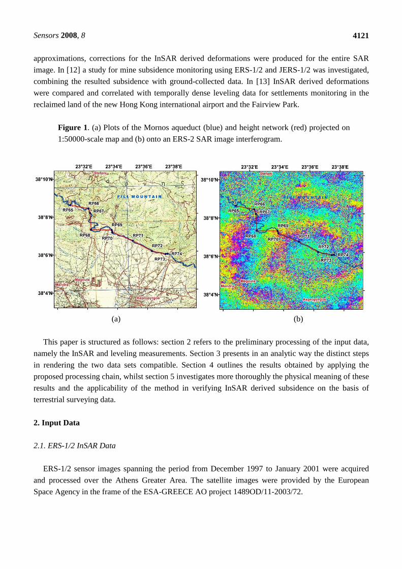
Figure 2. Set of interferometric pairs used in the study. The vertical dashed line indicates

the date of the earthquake occurrence.

-150

-100

-50

0

50

100

150

200

250

300

350

400

450

12/97 3/98 6/98 10/98 1/99 4/99 7/99 11/99 2/00 5/00 9/00 12/00

Alt

itu

de

of

am

big

uit

y (

m)

SAR image date

Interferometric calculations were done by using the CNES DIAPASON InSAR processing software,

and the sixteen most coherent co-seismic interferograms were kept for the purposes of the study. The

image pairs used along with their corresponding “altitude of ambiguities” are shown in Figure 2. The

influence of the terrain relief on the interferograms was lifted out using a DEM, which was originated

by digitizing the 20 m contour lines from the 1:50,000-scale topographic maps. The high frequency

DEM artifacts remaining in the interferograms, were calculated as the ratio of the DEM error (~10 m)

over the interferometric “altitude of ambiguity” (20 m–417 m) [14]. They were all estimated to be

below the cycle level (0.3–0.02 cycles).

2.2. Leveling Data Along the Mornos Aqueduct

The first terrestrial surveying work on the aqueduct was done in 1984, covering its whole length of

approximately 200 km. A special trigonometric height technique was used, providing the same level of

accuracy as conventional leveling but being significantly faster [15]. This technique employed a highly

accurate geodetic total station to obtain the slope distance and the vertical angle between the two points

of interest. The use of a redundant number of stationary sets of tripods and tribranch adapters

eliminated the need for target and instrument height measurements. Furthermore, atmospheric

refraction effects were further eliminated by concurrent measurements at both ends of an observation

line - leading to high accuracy observations.

Moreover, a standard geometric leveling was realized in 2001. The total distance surveyed was 40

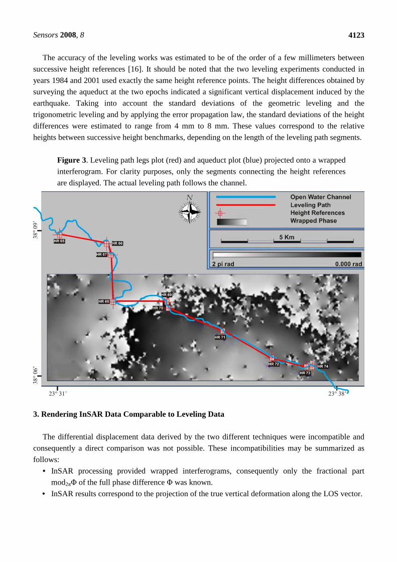
km, of which 12 km were confined in the area of interest illustrated in Figure 1(b). Figure 3 shows the

leveling path legs and the longitudinal axis of the open aqueduct, projected onto a wrapped

interferogram.

Sensors 2008, 8

4123

The accuracy of the leveling works was estimated to be of the order of a few millimeters between

successive height references [16]. It should be noted that the two leveling experiments conducted in

years 1984 and 2001 used exactly the same height reference points. The height differences obtained by

surveying the aqueduct at the two epochs indicated a significant vertical displacement induced by the

earthquake. Taking into account the standard deviations of the geometric leveling and the

trigonometric leveling and by applying the error propagation law, the standard deviations of the height

differences were estimated to range from 4 mm to 8 mm. These values correspond to the relative

heights between successive height benchmarks, depending on the length of the leveling path segments.

Figure 3. Leveling path legs plot (red) and aqueduct plot (blue) projected onto a wrapped

interferogram. For clarity purposes, only the segments connecting the height references

are displayed. The actual leveling path follows the channel.

3. Rendering InSAR Data Comparable to Leveling Data

The differential displacement data derived by the two different techniques were incompatible and

consequently a direct comparison was not possible. These incompatibilities may be summarized as

follows:

• InSAR processing provided wrapped interferograms, consequently only the fractional part

mod2πΦ of the full phase difference Φ was known.

• InSAR results correspond to the projection of the true vertical deformation along the LOS vector.

Sensors 2008, 8

4124

• The reference systems of the leveling data and the InSAR data were different. InSAR data were

referring to ED 50 UTM zone 34 while the leveling data were referring to the mean sea level and

the height reference positions to the Hellenic Geodetic Reference System 87 (HGRS 87).

• The interferograms were “noisy” mainly due to temporal decorrelation, orbital and tropospheric

disturbances. The following sections describe the procedure used to eliminate the effects of the above types of

incompatibility, rendering the two datasets comparable.

3.1. Wrapped Interferogram Filtering

The wrapped interferogram underwent a simple filtering procedure. The primary objective of this

action was to minimize the probability of phase unwrapping failure, while a secondary goal was the

improvement of the wrapped and unwrapped interferogram appearance in order to derive qualitative

evaluations more efficiently. The filter used was a simple 2D 3x3 space mean filter (symmetric to match the rectangular pixel dimensions), applied on both the real )cos( j,iψ and imaginary )sin( j,iψ

parts of a virtual unitary magnitude signal )sin(j)cos(e j,ij,ij j,i ψ+ψ=ψ . The phase of this signal is the

unfiltered interferometric phase j,iψ . In other words, the 2D space filter was applied on a unitary signal

to which the phase of the input interferogram was projected. The phase j,i/fltψ , comprising the filtered

interferogram, was extracted through an arctan operation from the filtered real and imaginary parts of

the virtual signal. The filtering procedure is best defined by the following formula:

ψψ=ψ ∑ ∑∑ ∑

−+=

−−=

−+=

−−=

−+=

−−=

−+=

−−=

2

1kjj

2

1kjj

2

1kii

2

1kii

2

j,i2

1kjj

2

1kjj

2

1kii

2

1kii

2

j,ij,i/flt

0

0

0

0

0

0

0

0

k

)cos(

k

)sin(arctan (1)

where k is the filter size, which equals 3. This value was considered to be an optimal one, as it

corresponds to a satisfactory tradeoff between interferometric spatial resolution and level of smoothing.

The criterion for choosing k was to eliminate isolated pixel noise while keeping the spatial deformation

trend evident in the interferogram. In Figure 4, the effect of the interferogram filtering procedure is

presented.

Figure 4. Wrapped interferogram, before (left) and after (right) filtering.

Sensors 2008, 8

4125

3.2. Phase Unwrapping

Various 2D phase unwrapping techniques have been developed for resolving the “integer

ambiguity” problem of the interferometric phases. In this study “Quality Guided Path Following”,

“Least Squares Without Weights”, “Weighted Least Squares”, and “Minimum LP Norm” approaches

were implemented [17-20]. The unwrapped interferograms produced by these techniques were

evaluated for surface discontinuities, by inspecting for the presence of breaklines (abrupt gradient

changes) or “tears” (non – derivabilities) and measuring their length. As a result, it was inferred that

the most effective technique, for this particular scenario, was the “Weighted Least Squares”. The

weights were derived from the coherence map, representing the computed cross correlation between

the master and the slave image.

The unwrapped co-seismic interferograms were all undergone a special processing in order to

minimize the existing orbital, tropospheric and DEM disturbances. These errors were lifted by a

“tilting” and “shifting” operation, using a number of coherent pixels located outside the deformed area.

According to this approach [21], the deformation on these pixels was expected to follow a well-defined

t-student distribution around a local zero mean. Then, by forcing each local deformation mean to zero,

the calculated interferograms were “tilted” and “sifted”. Figure 5 emphasizes the effect of this process,

where the disposal of the orbital fringes becomes evident.

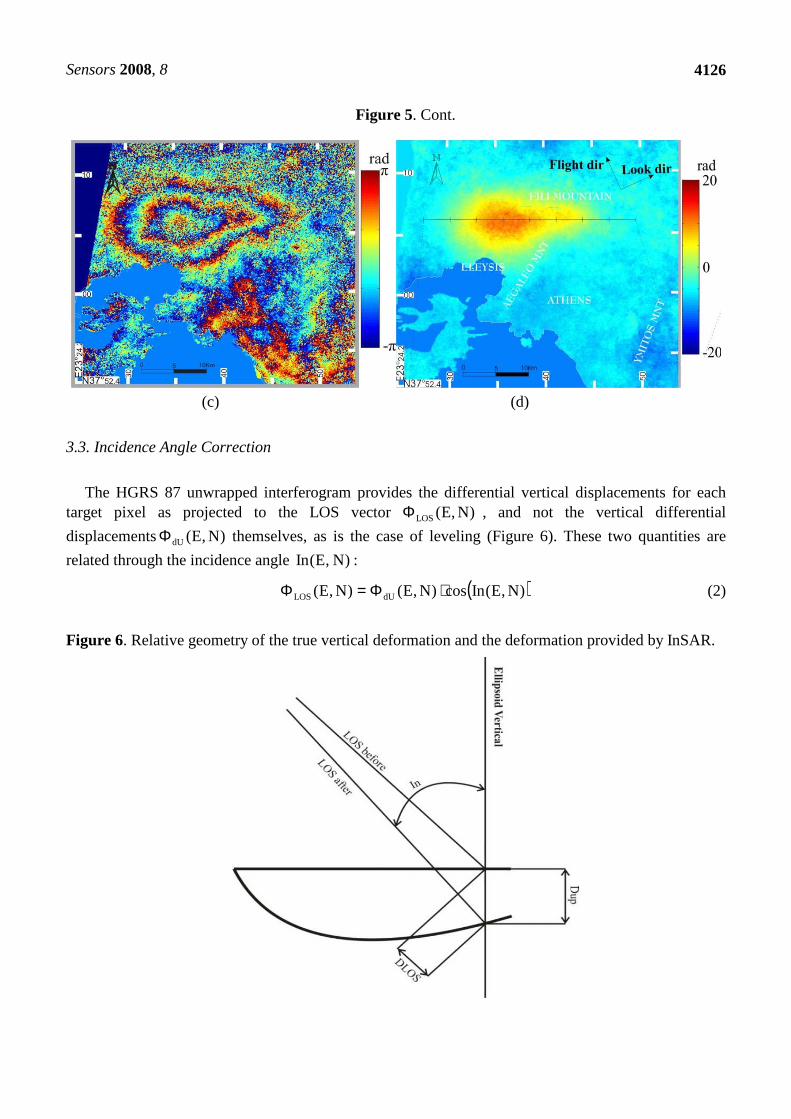
Figure 5. (a) & (b) Wrapped and unwrapped versions of the same interferogram. Note the

unrealistic fringe pattern due to inaccuracies in the orbital data used. (c) & (d) The effect

of the “tilting” and “shifting” operation on the same interferogram; the orbital fringes are

removed.

(a) (b)

Sensors 2008, 8

4126

Figure 5. Cont.

(c) (d)

3.3. Incidence Angle Correction

The HGRS 87 unwrapped interferogram provides the differential vertical displacements for each target pixel as projected to the LOS vector )N,E(LOSΦ , and not the vertical differential

displacements )N,E(dUΦ themselves, as is the case of leveling (Figure 6). These two quantities are

related through the incidence angle )N,E(In :

( ))N,E(Incos)N,E()N,E( dULOS ⋅Φ=Φ (2)

Figure 6. Relative geometry of the true vertical deformation and the deformation provided by InSAR.

Sensors 2008, 8

4127

In order to determine the differential vertical displacements from LOS projection displacements, the

value of the incidence angle for each target pixel was required. The incidence angle computation

procedure was based on satellite trajectory data and the position of the target. Initially, for every target

pixel (i, j) the zero - Doppler position of the space born SAR sensor had to be computed. This was

achieved through signal processing applied on the “master” (or “reference”) image. Third degree polynomials were fitted with Least Squares to the known satellite position vectors )t(r derived by ERS

1/2 operational orbits provided in the header file of every SAR image. These expressions simply

provide the satellite position vectors in the orbit’s terrestrial geocentric reference frame as a function of

time. Three polynomials were derived, one for every coordinate X, Y and Z. Exactly the same procedure was applied for the satellite velocity vector )(tr& and three additional equations were also

obtained. Therefore, for every single target (i, j) the following procedure was followed:

1. The map projection coordinates of the target were converted to geocentric Cartesian coordinates

in the geodetic terrestrial reference frame in which the satellite orbits were provided (in this

particular case from HGRS 87 map coordinates to ITRF 96 geocentric Cartesian coordinates).

2. The mean Doppler frequency shift was computed by the CNES DIAPASON software and was assumed to be the same for every single pixel target. The Doppler frequency shift ( )j,if was

expressed as a function of the satellite position, the satellite velocity vectors and the target position )j,i(r , by the following equation (λ denotes the SAR sensor wavelength):

( ) ( ))t()j,i(

)j,i()t()j,i(2j,if

i

i

rr

rrr

−λ⋅−

=&

(3)

3. A total of seven equations were accumulated, and an equal number of unknowns was introduced, three for the satellite position vector, three for the satellite velocity vector and one for the time it .

Hence, a non linear seven-equation system was created for the estimation of the seven unknowns.

The system was linearised with Taylor series expansion and solved iteratively.

4. Knowing the satellite and target position vectors, the unitary LOS vector could be calculated

simply from the following vector equation:

)t()j,i(

)t()j,i()j,i(

i

i

rr

rrLOS

−−

= (4)

5. The target position ellipsoidal coordinates j,iϕ , j,iλ were then calculated on the same geodetic

terrestrial frame, which was used to express the orbits and the target coordinates in the previous

step. 6. Knowing the target’s latitude and longitude j,iϕ , j,iλ , the LOS vector components were

transformed to the local geodetic reference system (delta north - DN, delta east - DE, delta up -

DU) by means of a rotation matrix:

( )

=λϕ

)t(DU

)t(DE

)t(DN

,R

)t(DZ

)t(DY

)t(DX

j,ij,i (5)

Sensors 2008, 8

4128

7. The third component of the LOS vector as expressed in the local geodetic reference system is

actually the direction cosine for the “up” axis of the system, and consequently the cosine of the

incidence angle In. Thus the incidence angle can be derived as:

( )DUarctanIn = (6)

3.4. Stacking

In the framework of this study and due to the fact that reliable verification data were available

through the leveling survey, it was possible to evaluate the advantage in using a mean stacked

interferogram instead of using only one, that is the “highest-quality” (most coherent) interferogram. For

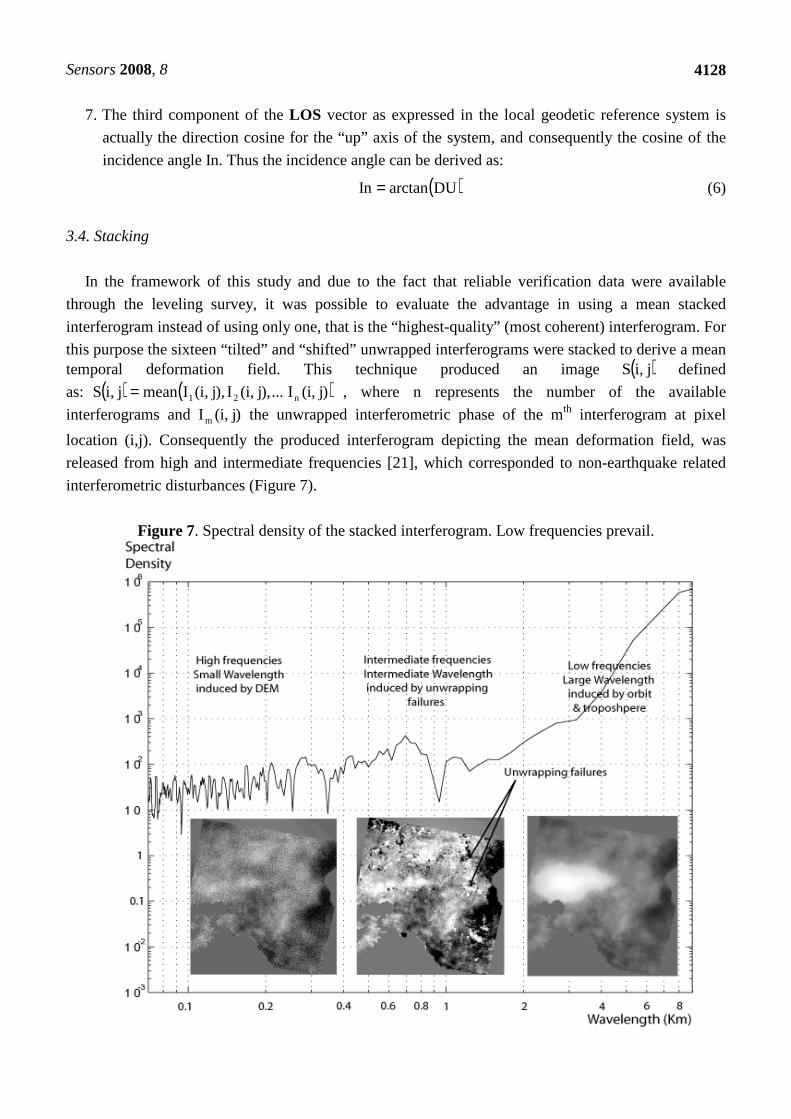
this purpose the sixteen “tilted” and “shifted” unwrapped interferograms were stacked to derive a mean temporal deformation field. This technique produced an image ( )j,iS defined

as: ( ) ( ))j,i(I...),j,i(I),j,i(Imeanj,iS n21= , where n represents the number of the available

interferograms and )j,i(I m the unwrapped interferometric phase of the mth interferogram at pixel

location (i,j). Consequently the produced interferogram depicting the mean deformation field, was

released from high and intermediate frequencies [21], which corresponded to non-earthquake related

interferometric disturbances (Figure 7).

Figure 7. Spectral density of the stacked interferogram. Low frequencies prevail.

Sensors 2008, 8

4129

It should be mentioned that at this stage alternative stacking methods were implemented as well.

They comprised of the formation of A) a weighted mean stacked interferogram, using as weights the

pixel coherence values of each contributing interferogram, B) a maximum coherence stacked product,

on which each phase pixel value stems from the interferogram with the highest corresponding

coherence pixel value and C) a windowed maximum coherence stacked product; here each phase pixel

value stems from the interferogram with the highest mean coherence value, calculated inside a 3 by 3

pixels window, centered on the pixel of interest. As is shown in section 4, the above methods returned

very similar results compared to the mean stacked approach.

3.5. Geodetic Reference System Conversion

As mentioned the unwrapped interferometric calculations were referring to a UTM map projection

on the ED 50 Greek Datum. In contrast the coordinates of the height references were expressed in the

HGRS 87 reference system, using the Transverse Mercator map projection on the GRS 80 ellipsoid. To

overcome this incompatibility the initial interferograms were converted to HGRS 87 projection system

as follows:

1. The ED 50 UTM map coordinates (Eastings and Northings - E, N) were converted to ED 50

ellipsoidal coordinates (latitude and longitude - φ, λ), assigning to each pixel the corresponding

orthometric height (Η) derived from the input DEM.

2. The orthometric heights were converted to geometric ones (h), by implementing a constant

additive geoid undulation value (N) for the entire area of interest, since the geoid in this area is

relatively “flat” exhibiting a very low gradient. This value was obtained by the Ohio State

University OSU 91 Geoid Model, and was recomputed for ED 50.

3. The ED 50 ellipsoidal coordinates were converted to ED 50 Cartesian coordinates (X, Y, Z).

4. Subsequently, the ED 50 geocentric Cartesian coordinates were converted to HGRS 87

geocentric ones, assuming only a parallel shift between the two systems. The latter assumption

was expected to successfully provide the conversion due to the small size of the area of interest.

5. Then, the HGRS 87 geocentric Cartesian coordinates were translated to HGRS 87 ellipsoidal (φ,

λ) coordinates.

6. Ultimately, the HGRS 87 ellipsoidal (φ, λ) coordinates were converted to HGRS 87 Transverse

Mercator projection coordinates (E, N).

3.6. Differential Vertical Displacement Modeling

Thorough examination of the unwrapped (stacked and/or “highest-quality”) interferograms,

exhibited the presence of “local” phase anomalies in certain areas extending from one to several pixels.

The phase values in these pixels deviated from the prevailing values in the surrounding region. These

anomalies were survived the filtering procedure described in section 3.1. It is beyond the scope of this

paper to explore the origin of such phase “residuals”, but it could be assumed that they stemmed from

local temporal decorrelation. It was also observed that the areas affected by these anomalies, presented

significantly low coherence values and therefore they should be excluded.

Sensors 2008, 8

4130

Because the tectonic deformations observed were characterized by low phase gradient and spatial

continuity, it was decided to proceed with a phase smoothing operation, by fitting (with the Weighted

Least Squares method) a 3D-mathematical surface to the unwrapped interferometric phases )N,E(dUΦ . After a series of adjustments, a successful fit according to the chi-square )( 2χ test was

achieved, using the value of 6 mm as a-priori standard deviation for the observations. By the

application of the error propagation law (given the estimated model parameters and their a-posteriori

standard deviation values), it was concluded that the 3D-mathematical surface would provide the

vertical deformation estimate for each target pixel (E, N), with an estimated a-priori deviation not

higher than 0.2 mm. In order to ensure that the mathematical model represents the best fit to the

displacement pattern observed, the most general form of mth degree surface was tested:

( )( )

( )( )

( )( )

++

++++

++++

−=Φ−−−

−−−

11mNE

2m2NE

1m1NE

11EN

mN

2N

1N

mE

2E

1E0

dU

NEa...NEaNEa

NEaNa...NaNa

Ea...EaEaa

)N,E(

11m2m21m1

m21

m21

(7)

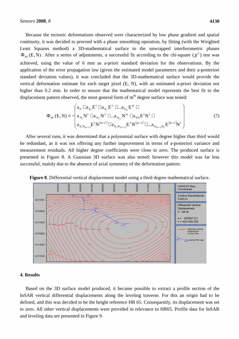
After several runs, it was determined that a polynomial surface with degree higher than third would

be redundant, as it was not offering any further improvement in terms of a-posteriori variance and

measurement residuals. All higher degree coefficients were close to zero. The produced surface is

presented in Figure 8. A Gaussian 3D surface was also tested; however this model was far less

successful, mainly due to the absence of axial symmetry of the deformation pattern.

Figure 8. Differential vertical displacement model using a third degree mathematical surface.

4. Results

Based on the 3D surface model produced, it became possible to extract a profile section of the

InSAR vertical differential displacements along the leveling traverse. For this an origin had to be

defined, and this was decided to be the height reference HR 65. Consequently, its displacement was set

to zero. All other vertical displacements were provided in relevance to HR65. Profile data for InSAR

and leveling data are presented in Figure 9.

Sensors 2008, 8

4131

Examining the profiles illustrated in Figure 9, it can be concluded that no major differences occur

between the differential vertical displacements as obtained by InSAR and leveling. There appears to be

an agreement between the two profiles with respect to the gradient of the vertical displacement. Also

there is no evidence of any systematic deviation between them. Moreover the profile corresponding to

the mean stacked interferogram shows a better agreement with the leveling data. The vertical

displacement differences between the leveling data and the interferometric data using the “highest

quality” interferogram range from 3 mm up to 1.8 cm. The average difference value between the two

data sets is 9.5 mm and the standard deviation equals 5.5 mm. On the contrary, when the mean stacked

interferogram is compared with the leveling data, the above discrepancies are reduced by a factor of

six. Indeed, the average difference between the two data sets is reduced down to 1.5 mm, whereas the

standard deviation is of the order of 4.8 mm.

Figure 9. Differential vertical deformation profiles derived by the, (a) conventional

terrestrial surveying, (b) single “highest quality” interferogram, (c) mean stacked

interferogram, (d) windowed maximum coherence interferogram. HR65 indicates the

starting point of leveling.

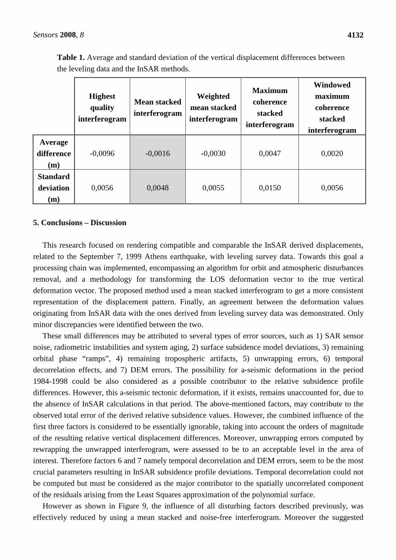
Table 1 outlines the average vertical displacement difference between the leveling data and the

interferometric data for the various interferometric approaches used. The study of the table shows that

the mean stacked product is preferred against the other interferograms, as it fits precisely the leveling

data. Also its estimation entails less computational complexity. It should be mentioned though, that

there are no major differences between the various stacking methods. However, significant

improvement was achieved when moving from the single most coherent interferogram to any of the

stacked products.

Sensors 2008, 8

4132

Table 1. Average and standard deviation of the vertical displacement differences between

the leveling data and the InSAR methods.

Highest quality

interferogram

Mean stacked interferogram

Weighted mean stacked interferogram

Maximum coherence stacked

interferogram

Windowed maximum coherence stacked

interferogram

Average difference

(m)

-0,0096 -0,0016 -0,0030 0,0047 0,0020

Standard deviation

(m)

0,0056 0,0048 0,0055 0,0150 0,0056

5. Conclusions – Discussion

This research focused on rendering compatible and comparable the InSAR derived displacements,

related to the September 7, 1999 Athens earthquake, with leveling survey data. Towards this goal a

processing chain was implemented, encompassing an algorithm for orbit and atmospheric disturbances

removal, and a methodology for transforming the LOS deformation vector to the true vertical

deformation vector. The proposed method used a mean stacked interferogram to get a more consistent

representation of the displacement pattern. Finally, an agreement between the deformation values

originating from InSAR data with the ones derived from leveling survey data was demonstrated. Only

minor discrepancies were identified between the two.

These small differences may be attributed to several types of error sources, such as 1) SAR sensor

noise, radiometric instabilities and system aging, 2) surface subsidence model deviations, 3) remaining

orbital phase “ramps”, 4) remaining tropospheric artifacts, 5) unwrapping errors, 6) temporal

decorrelation effects, and 7) DEM errors. The possibility for a-seismic deformations in the period

1984-1998 could be also considered as a possible contributor to the relative subsidence profile

differences. However, this a-seismic tectonic deformation, if it exists, remains unaccounted for, due to

the absence of InSAR calculations in that period. The above-mentioned factors, may contribute to the

observed total error of the derived relative subsidence values. However, the combined influence of the

first three factors is considered to be essentially ignorable, taking into account the orders of magnitude

of the resulting relative vertical displacement differences. Moreover, unwrapping errors computed by

rewrapping the unwrapped interferogram, were assessed to be to an acceptable level in the area of

interest. Therefore factors 6 and 7 namely temporal decorrelation and DEM errors, seem to be the most

crucial parameters resulting in InSAR subsidence profile deviations. Temporal decorrelation could not

be computed but must be considered as the major contributor to the spatially uncorrelated component

of the residuals arising from the Least Squares approximation of the polynomial surface.

However as shown in Figure 9, the influence of all disturbing factors described previously, was

effectively reduced by using a mean stacked and noise-free interferogram. Moreover the suggested

Sensors 2008, 8

4133

tilting and shifting procedure, introduced in [21], for removing orbital and tropospheric fringes has

performed effectively. Hence, the earthquake induced subsidence pattern seemed to be successfully

represented by the proposed model.

As far as the terrestrial surveying derived relative subsidence profiles are concerned, the estimation

accuracy was much simpler and more explicit. The leveling data accuracy was estimated to lie in the

range from 4 mm to 8 mm, in relative heights between successive height benchmarks. With the above

estimations it becomes clear that the deviation of the two relative subsidence profiles (cases (a) and (c)

in Figure 9), fall entirely within the confidence interval defined for the leveling data. It can be also

concluded that the simple polynomial surface modeling of the subsidence field, may be regarded as an

effective method to overcome the remaining temporal decorrelation effects and other sources of noise,

by exploiting the extremely high degrees of freedom associated with the Least Squares approximation

of mathematical models. Finally, a case specific conclusion of geophysical interest can be drawn for

the study area. This refers to the fact that no detectable significant vertical displacements have occurred

during the period 1984-1998, for which InSAR interferometric measurements were not available.

Acknowledgements

We are grateful to the European Space Agency (ESA) for providing us the ERS1/2 data, in the

framework of the ESA-GREECE AO project 1489OD/11-2003/72.

References 1. Kontoes, C.; Elias, P.; Sykioti, O.; Briole, P.; Remy, D.; Sachpazi, M.; Veis, G.; Kotsis, I.

Displacement Field Mapping and Fault Modeling of the Mw = 5.9, September 7, 1999 Athens

Earthquake based on ERS-2 Satellite RADAR Interferometry. Geophysical Research Letters

2000, 27, 3989-3992.

2. Roumelioti, Z; Dreger, D.; Kiratzi, A.; Theodoulidis, N. Slip distribution of the 7 September 1999

Athens earthquake inferred from an empirical Green’s function study. Bulletin of the

Seismological Society of America 2003, 93, 775-782.

3. Baumont, D.; Courboulex, F.; Scotti, O.; Melis, N.S.; Stavrakakis, G. Slip distribution of the M-w

5.9, 1999 Athens earthquake inverted from regional seismological data. Geophysical Research

Leters 2002, 29, 1720.

4. Papadimitriou, P.; Voulgaris, N.; Kassaras, I.; Kaviris, G.; Delibasis, N.; Makropoulos, K. The M-

w=6.0, 7 September 1999 Athens earthquake. Natural Hazards 2002, 27, 15-33.

5. Sargeant, S.L.; Burton, P.W.; Douglas, A.; Evans, J.R. The source mechanism of the Athens

earthquake, September 7, 19999, estimated from P seismograms recorded at long range. Natural

Hazards 2002, 27, 33-45.

6. Pavlides, S.B.; Papadopoulos, G.; Ganas, A. The fault that caused the Athens September 1999

Ms=5.9 earthquake: Field observations. Natural Hazards 2002, 27, 61-84.

7. Goldsworthy, M.; Jackson, J.; Hains, J. The continuity of the active fault systems in Greece.

Geophysical Journal International 2002, 148, 596-618.

Sensors 2008, 8

4134

8. Bouckovalas, G.D.; Kouretzis, G.P. Stiff soil amplification effects in the 7 September 1999

Athens (Greece) earthquake. Soil Dynamics and Earthquake Engineering 2001, 21, 671-687.

9. Eftaxias, K.; Kapiris, P.; Polygiannakis, J.; Borgis, N.; Kopanas, J.; Antonopoulos, G.; Peratzakis,

A.; Hadjicontis, V. Signature of pending earthquake from electromagnetic anomalies. Geophysical

Research Letters 2001, 28, 3321-3324.

10. Odijk, D.; Kenselaar, F.; Hanssen, R. Integration of Leveling and InSAR Data For Land

Subsidence Monitoring. In Proc. 11th International FIG Symposium on Deformation

Measurements 2003; Commission 6, Santorini Island, Greece, 8.

11. Zhou, Y.; Stein, A.; Molenaar, M. Integrating Interferometric SAR data with Leveling

Measurements of Land Subsidence Using Geostatistics. International Journal of Remote Sensing

2003, 24, 3547-3564.

12. Ge, L.; Chang, H.C.; Janssen, V.; Rizos, C. The Integration of GPS, radar Intrerferometry and GIS

for Ground Deformation Monitoring. In Proc. Int. Symposium on GPS/GNSS 2003, Tokyo, Japan;

pp. 465-472.

13. Liu, G.; Chen, Y.; Ding, X.; Li, Z.; Li, Z.W. Monitoring Ground Settlement in Hong Kong with

Satellite SAR Interferometry. In Proc. FIG XXII International Congress Washington 5; 2002,

JS17, 12.

14. Massonet, D.; Feigl, K.; Radar interferometry and its application to changes in the Earth’s surface.

Reviews of Geophysics 1998, 36, 441-500.

15. Balodimos, D. The development of a special trigonometric leveling technique. Tecnika chronic

1979, 3 (in Greek).

16. Deltsidis, P.; Saridakis, M. Displacement determination with terrestrial and satellite methods.

Diploma Thesis, 2001, Dionysos Satellite Observatory, National Technical University of Athens

(in Greek).

17. Prit, M.D. Comparison of path-following and least-squares phase unwrapping algorithms. IGARSS 1997, 2, 872-875.

18. Zebker, H.A.; Lu, Y. Phase unwrapping algorithms for radar interferometry: Residue-cut, least

squares, and synthesis algorithms. Journal of the Optical Society of America 1998, 15, 586-598.

19. Pritt, M.D. Congruence in least-squares phase unwrapping. IGARSS 1997, 2, 875-877.

20. Ghiglia, D.C.; Romero, L.A. Minimum LP-norm two-dimensional phase unwrapping. Journal of

the Optical Society of America 1996, 13, 1999-2013.

21. Elias, P.; Kontoes, C.; Sykioti, O.; Avallone, A.; Briole, P.; Paradissis, D. A method for

minimizing low frequency and unwrapping artefacts from interferometric calculations.

International Journal of Remote Sensing 2006, 27, 3079-3086.

© 2008 by the authors; licensee Molecular Diversity Preservation International, Basel, Switzerland.

This article is an open-access article distributed under the terms and conditions of the Creative

Commons Attribution license (http://creativecommons.org/licenses/by/3.0/).