insar - utah subsidence in southwest utah from 1993 to 1998 measured with interferometric synthetic...

Land subsidence in southwest Utah from 1993 to 1998 measured with Interferometric Synthetic Aperture Radar (InSAR)

by Richard R. Forster

InSA

R

MISCELLANEOUS PUBLICATION 06-5

UTAH GEOLOGICAL SURVEY a division of

Utah Department of Natural Resources

2006

Land subsidence in southwest Utah from 1993 to 1998 measured with Interferometric

Synthetic Aperture Radar (InSAR)

by Richard R. Forster

University of Utah, Department of Geography, Salt Lake City, Utah

MISCELLANEOUS PUBLICATION 06-5 UTAH GEOLOGICAL SURVEY a division of Utah Department of Natural Resources

2006

ISBN 1-55791-754-X

STATE OF UTAHJon Huntsman, Jr., Governor

DEPARTMENT OF NATURAL RESOURCESMichael Styler, Executive Director

UTAH GEOLOGICAL SURVEYRichard G. Allis, Director

PUBLICATIONScontact

Natural Resources Map/Bookstore1594 W. North Temple

Salt Lake City, UT 84116telephone: 801-537-3320

toll-free: 1-888-UTAH MAPwebsite: http://mapstore.utah.gov

email: [email protected]

THE UTAH GEOLOGICAL SURVEYcontact

1594 W. North Temple, Suite 3110Salt Lake City, UT 84116telephone: 801-537-3300

fax: 801-537-3400web: http://geology.utah.gov

The Miscellaneous Publication series provides non-UGS authors with a high-quality format for documents concerning Utah geology. Althoughreview comments have been incorporated, this publication does not necessarily conform to UGS technical, policy, or editorial standards.

The Utah Department of Natural Resources, Utah Geological Survey, makes no warranty, expressed or implied, regarding the suitability of this prod-uct for a particular use. The Utah Department of Natural Resources, Utah Geological Survey, shall not be liable under any circumstances for anydirect, indirect, special, incidental, or consequential damages with respect to claims by users of this product.

The Utah Department of Natural Resources receives federal aid and prohibits discrimination on the basis of race, color, sex, age, national origin,or disability. For information or complaints regarding discrimination, contact Executive Director, Utah Department of Natural Resources, 1594West North Temple #3710, Box 145610, Salt Lake City, UT 84116-5610 or Equal Employment Opportunity Commission, 1801 L. Street, NW,Washington, DC 20507.

10/06

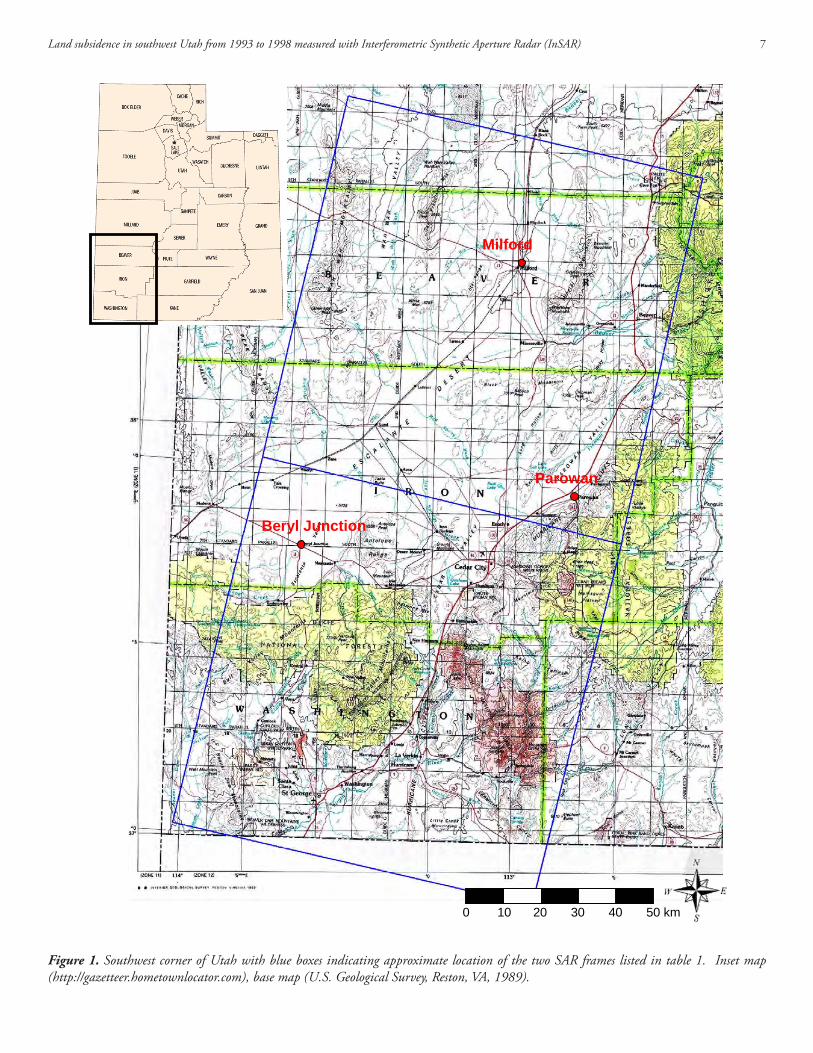
FIGURESFigure 1. Southwest corner of Utah with blue boxes indicating approximate location of the two SAR frames listed in table 1. Inset

map (http://gazetteer.hometownlocator.com), Base map (Interior Geological Survey, Reston, VA, 1989.) ................................... 8Figure 2a. Interferogram from SAR frames acquired on 02/27/1993 and 02/05/1996 with topography and baseline contributions

removed (each cycle of color corresponds to 2.8 cm of radar line-of-sight displacement) over grayscale SAR power image. ......... 9Figure 2b. Interferogram from SAR frames acquired on 02/27/1993 and 02/06/1996 with topography and baseline contributions

removed (each cycle of color corresponds to 2.8 cm of radar line-of-sight displacement) over grayscale SAR power image. ....... 10Figure 2c. Interferogram from SAR frames acquired on 02/05/1996 and 03/17/1998 with topography and baseline contributions

removed (each cycle of color corresponds to 2.8 cm of radar line-of-sight displacement) over grayscale SAR power image. ....... 11Figure 2d. Interferogram from SAR frames acquired on 02/06/1996 and 03/17/1998 with topography and baseline contributions

removed (each cycle of color corresponds to 2.8 cm of radar line-of-sight displacement) over grayscale SAR power image. ....... 12Figure 3a. Detailed portion of interferogram for Escalante Valley from SAR frames acquired on top: 02/27/1993 and 02/05/1996,

and bottom: 02/27/1993 and 02/06/1996. Numbers are the acquisition dates of the InSAR pairs (table 2). ............................ 13Figure 3b. Detailed portion of interferogram for Milford area from SAR frames acquired on top: 02/27/1993 and 02/05/1996, and

bottom: 02/27/1993 and 02/06/1996. Numbers are the acquisition dates of the InSAR pairs (table 2). .................................. 14Figure 3c. Detailed portion of interferogram for Parowan area from SAR frames acquired at right: 02/27/1993 and 02/05/1996, and

left: 02/27/1993 and 02/06/1996. Numbers are the acquisition dates of the InSAR pairs (table 2). ......................................... 15Figure 4a. Detailed portion of interferogram for Escalante Valley from SAR frames acquired on top: 02/05/1996 and 03/17/1998,

and bottom: 02/06/1996 and 03/17/1998. Numbers are the acquisition dates of the InSAR pairs (table 2). ............................ 16Figure 4b. Detailed portion of interferogram for the Milford area from SAR frames acquired on top: 02/05/1996 and 03/17/1998,

and bottom: 02/06/1996 and 03/17/1998. Numbers are the acquisition dates of the InSAR pairs (table 2). ............................ 17Figure 4c. Detailed portion of interferogram for the Parowan area from SAR frames acquired on top: 02/05/1996 and 03/17/1998,

and bottom: 02/06/1996 and 03/17/1998. Numbers are the acquisition dates of the InSAR pairs (table 2). ............................ 18Figure 5a. Vertical displacement map of the Escalante Valley area from InSAR pair 02/27/1993 - 02/05/1996 as opaque color over

Landsat ETM+ band 4 in grayscale. Negative values indicate surface lowering relative to bedrock. .......................................... 19Figure 5b. Vertical displacement map of the Escalante Valley from InSAR pair 02/05/1996 - 03/17/1998 as opaque color over Land-

sat ETM+ band 4 in grayscale. Negative values indicate surface lowering relative to bedrock. .................................................. 20Figure 5c. Vertical displacement map of the Escalante Valley from the sum of figures 5a and 5b as opaque color over Landsat ETM+

TABLE OF CONTENTSABSTRAcT ...................................................................................................................................................................................... 1

INTRoDUcTIoN .......................................................................................................................................................................... 1

objective ..................................................................................................................................................................................... 1

Data Set ...................................................................................................................................................................................... 1

PRocESSING .................................................................................................................................................................................. 2

RESULTS AND ANALySIS ............................................................................................................................................................. 2

Escalante Valley ........................................................................................................................................................................... 3

Milford ........................................................................................................................................................................................ 5

Parowan ...................................................................................................................................................................................... 5

coNcLUSIoNS AND REcoMMENDATIoNS ........................................................................................................................ 5

AckNowLEDGMENTS................................................................................................................................................................ 6

REFERENcES ................................................................................................................................................................................. 6

band 4 in grayscale. Negative values indicate surface lowering relative to bedrock. ................................................................... 21Figure 6a. Subsidence rate map of the Escalante Valley area from InSAR pair 02/27/1993 - 02/05/1996 as opaque color over Landsat

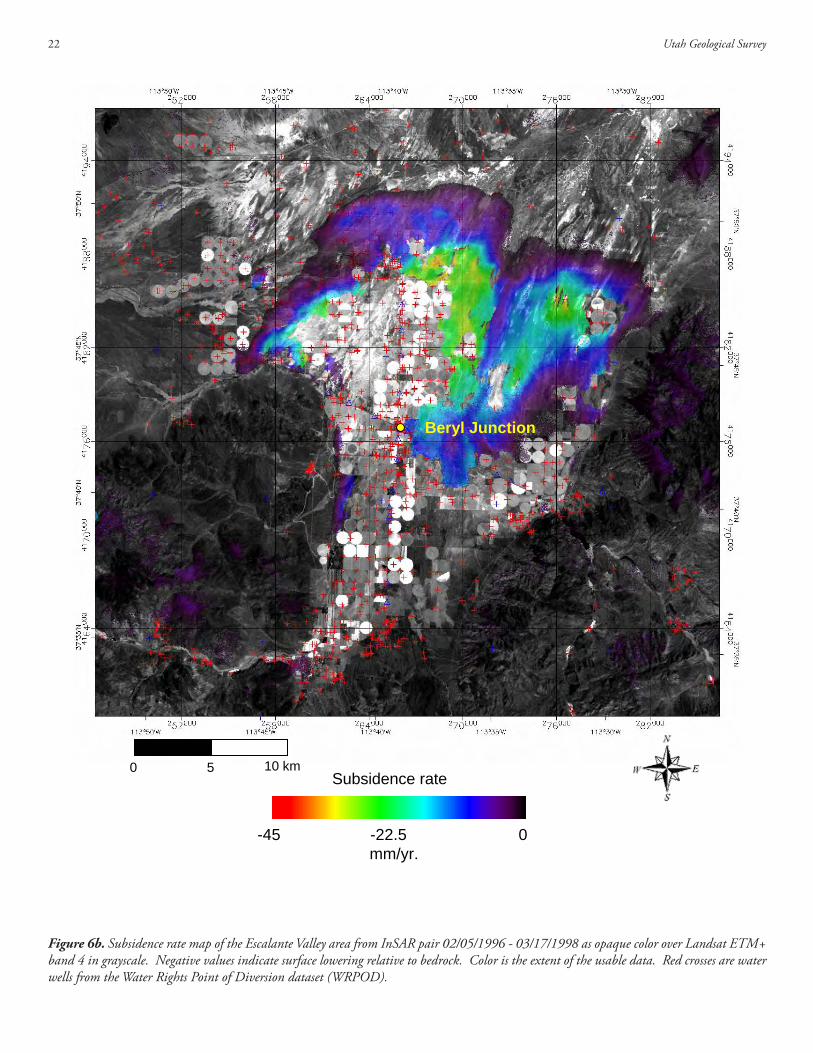
ETM+ band 4 in grayscale. Negative values indicate surface lowering relative to bedrock. ........................................................ 22Figure 6b. Subsidence rate map of the Escalante Valley area from InSAR pair 02/05/1996 - 03/17/1998 as opaque color over Landsat

ETM+ band 4 in grayscale. Negative values indicate surface lowering relative to bedrock. ....................................................... 23Figure 6c. Subsidence rate map of the Escalante Valley area from the sum of figures 6a and 6b as opaque color over Landsat ETM+

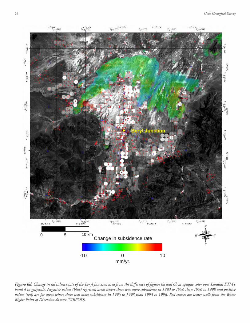
band 4 in grayscale. Negative values indicate surface lowering relative to bedrock. ................................................................... 24Figure 6d. change in subsidence rate of the Beryl Junction area from the difference of figures 6a and 6b as opaque color over Landsat

ETM+ band 4 in grayscale. Negative values (blue) represent areas where there was more subsidence in 1993 to 1996 than 1996 to 1998 and positive values (red) are for areas where there was more subsidence in 1996 to 1998 than 1993 to 1996. Red crosses are water wells from the water Rights Point of Diversion dataset (wRPoD). ........................................................................... 25

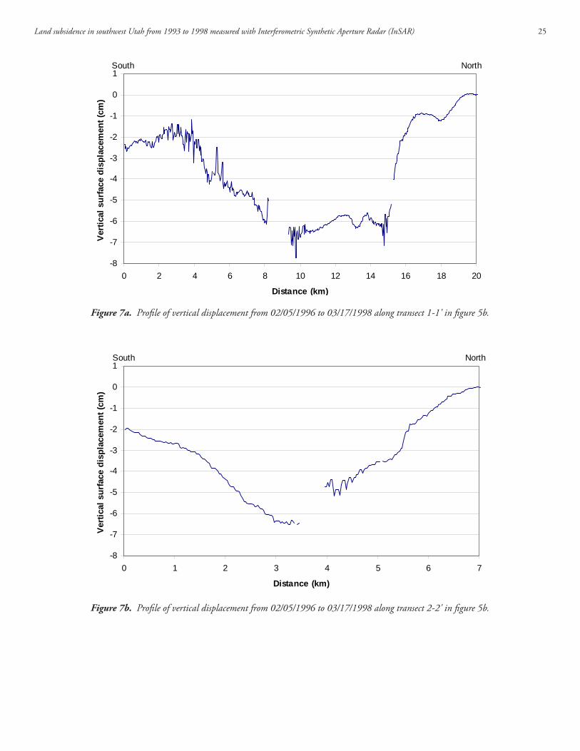
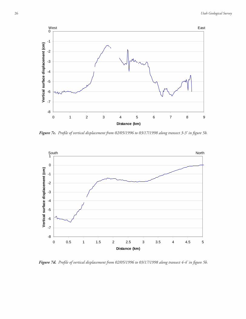
Figure 7a. Profile of vertical displacement from 02/05/1996 to 03/17/1998 along transect 1-1' in figure 5b. .................................. 26Figure 7b. Profile of vertical displacement from 02/05/1996 to 03/17/1998 along transect 2-2' in figure 5b. ................................. 26Figure 7c. Profile of vertical displacement from 02/05/1996 to 03/17/1998 along transect 3-3' in figure 5b. .................................. 27Figure 7d. Profile of vertical displacement from 02/05/1996 to 03/17/1998 along transect 4-4' in figure 5b. .................................. 27Figure 8. Vertical displacement map of the Escalante Valley from InSAR pair 02/05/1996 - 03/17/1998 as opaque color over Landsat

ETM+ band 4 in grayscale. Negative values indicate surface lowering relative to bedrock. ....................................................... 28Figure 9a. Vertical displacement map of the Milford area from InSAR pair 02/27/1993 - 02/05/1996 as opaque color over Landsat

ETM+ band 4 in grayscale. Negative values indicate surface lowering relative to bedrock. ....................................................... 29Figure 9b. Vertical displacement map of the Milford area from InSAR pair 02/05/1996 - 03/17/1998 as opaque color over Landsat

ETM+ band 4 in grayscale. Negative values indicate surface lowering relative to bedrock. ....................................................... 30Figure 9c. Vertical displacement map of the Milford area from the sum of figures 9a and 9b as opaque color over Landsat ETM+

band 4 in grayscale. Negative values indicate surface lowering relative to bedrock. ................................................................... 31

ABSTRACTLand subsidence in southwest Utah was measured with inter-ferometric synthetic aperture radar (InSAR). SAR acquisitions separated by up to 35 months from the European Space Agency’s (ESA) ERS-1 and ERS-2 satellites produced subsidence maps in areas immediately surrounding agricultural fields. of the three ar-eas investigated, Escalante Valley had the greatest magnitude and spatial extent of subsidence compared to the Milford and Parowan areas. The maximum total subsidence measured with InSAR in the Escalante Valley was 17 centimeters from February 1993 to March 1998. In this area the subsidence rate of 3 to 4 centime-ters per year is generally consistent between the two time periods measured (1993 to 1996 and 1996 to 1998) with isolated areas of change. This subsidence rate is consistent with a GPS-based sub-sidence rate estimate of 3 centimeters per year near Beryl Junction for the period 1941 to 1972. To increase the spatial and temporal extent of the subsidence maps, in this and other areas in Utah, a newer “persistent scatterers” InSAR technique is recommended along with multiple SAR acquisitions per year.

INTRODUCTION

Objective

The objective of this study is to measure land-surface subsidence in southwest Utah using Interferometric Synthetic Aperture Radar (InSAR). During the winter of 2004/2005, the Utah Geological Survey (UGS) documented earth fissures near Beryl Junction in Iron county, Utah (Lund and others, 2005). The UGS conclud-ed that these fissures formed due to ground-water withdrawal in the area, which has caused compaction in the Escalante Valley aquifer and ground subsidence near Beryl Junction (Lund and others, 2005). This study will use InSAR to measure potential

surface displacement in the Escalante Valley and investigate other locations of potential subsidence, specifically in the Parowan and Milford areas.

The InSAR technique can measure centimeter-scale surface dis-placement from a pair of SAR images acquired at different times. The time lapse between the acquisitions can be days to years. The surface change is computed by measuring the difference in distance from each of the two satellite positions to the ground for every pixel in the SAR image. This difference in distance is measured indirectly by the phase difference of the returned radar signal at each pixel. After InSAR processing, the pixels represent approximately 30-meters squares.

Data Set

The SAR data used in this study were acquired by the European Space Agency’s (ESA) ERS-1 and ERS-2 satellites. Two consecu-tive 100 x 100 kilometer frames from the same orbit were used to obtain the spatial coverage required for the three areas of interest (figure 1). A pair of consecutive frames will be referred to as a single scene for this document for simplicity and because the two frames were concatenated and processed as a single scene.

The six SAR scenes were obtained from ESA to measure potential spatial and temporal changes in the land-surface deformation pat-tern (table 1). The scenes selected have acquisition dates during winter to minimize the effects of changes in the agricultural land cover during the growing season. A previous UGS report for this area showed that the InSAR signal is less stable when one of the SAR acquisitions is during the growing season and in late winter when the soil is likely frozen, the crops have been harvested, the ground conditions are likely the most stable (Forster, 2005). The six scenes selected from the ESA data catalogue represent the best combination of winter acquisitions that progressively span the longest time interval with reasonable imaging geometry.

LAND SUBSIDENCE IN SOUTHwEST UTAH FROM 1993 TO 1998 MEASURED wITH INTERFEROMETRIC

SYNTHETIC APERTURE RADAR (INSAR)

by Richard R. Forster University of Utah, Department of Geography, Salt Lake City, Utah

Utah Geological Survey2

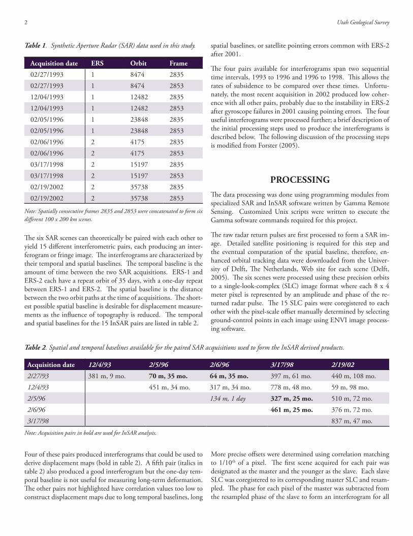
Table 1. Synthetic Aperture Radar (SAR) data used in this study.

Acquisition date ERS Orbit Frame

02/27/1993 1 8474 283502/27/1993 1 8474 285312/04/1993 1 12482 283512/04/1993 1 12482 285302/05/1996 1 23848 283502/05/1996 1 23848 285302/06/1996 2 4175 283502/06/1996 2 4175 285303/17/1998 2 15197 283503/17/1998 2 15197 285302/19/2002 2 35738 283502/19/2002 2 35738 2853

Note: Spatially consecutive frames 2835 and 2853 were concatenated to form six different 100 x 200 km scenes.

The six SAR scenes can theoretically be paired with each other to yield 15 different interferometric pairs, each producing an inter-ferogram or fringe image. The interferograms are characterized by their temporal and spatial baselines. The temporal baseline is the amount of time between the two SAR acquisitions. ERS-1 and ERS-2 each have a repeat orbit of 35 days, with a one-day repeat between ERS-1 and ERS-2. The spatial baseline is the distance between the two orbit paths at the time of acquisitions. The short-est possible spatial baseline is desirable for displacement measure-ments as the influence of topography is reduced. The temporal and spatial baselines for the 15 InSAR pairs are listed in table 2.

Table 2. Spatial and temporal baselines available for the paired SAR acquisitions used to form the InSAR derived products.

Acquisition date 12/4/93 2/5/96 2/6/96 3/17/98 2/19/02

2/27/93 381 m, 9 mo. 70 m, 35 mo. 64 m, 35 mo. 397 m, 61 mo. 440 m, 108 mo. 12/4/93 451 m, 34 mo. 317 m, 34 mo. 778 m, 48 mo. 59 m, 98 mo.2/5/96 134 m, 1 day 327 m, 25 mo. 510 m, 72 mo.2/6/96 461 m, 25 mo. 376 m, 72 mo.3/17/98 837 m, 47 mo.

Note: Acquisition pairs in bold are used for InSAR analysis.

Four of these pairs produced interferograms that could be used to derive displacement maps (bold in table 2). A fifth pair (italics in table 2) also produced a good interferogram but the one-day tem-poral baseline is not useful for measuring long-term deformation. The other pairs not highlighted have correlation values too low to construct displacement maps due to long temporal baselines, long

spatial baselines, or satellite pointing errors common with ERS-2 after 2001.

The four pairs available for interferograms span two sequential time intervals, 1993 to 1996 and 1996 to 1998. This allows the rates of subsidence to be compared over these times. Unfortu-nately, the most recent acquisition in 2002 produced low coher-ence with all other pairs, probably due to the instability in ERS-2 after gyroscope failures in 2001 causing pointing errors. The four useful interferograms were processed further; a brief description of the initial processing steps used to produce the interferograms is described below. The following discussion of the processing steps is modified from Forster (2005).

PROCESSINGThe data processing was done using programming modules from specialized SAR and InSAR software written by Gamma Remote Sensing. customized Unix scripts were written to execute the Gamma software commands required for this project.

The raw radar return pulses are first processed to form a SAR im-age. Detailed satellite positioning is required for this step and the eventual computation of the spatial baseline, therefore, en-hanced orbital tracking data were downloaded from the Univer-sity of Delft, The Netherlands, web site for each scene (Delft, 2005). The six scenes were processed using these precision orbits to a single-look-complex (SLc) image format where each 8 x 4 meter pixel is represented by an amplitude and phase of the re-turned radar pulse. The 15 SLc pairs were coregistered to each other with the pixel-scale offset manually determined by selecting ground-control points in each image using ENVI image process-ing software.

More precise offsets were determined using correlation matching to 1/10th of a pixel. The first scene acquired for each pair was designated as the master and the younger as the slave. Each slave SLc was coregistered to its corresponding master SLc and resam-pled. The phase for each pixel of the master was subtracted from the resampled phase of the slave to form an interferogram for all

Land subsidence in southwest Utah from 1993 to 1998 measured with Interferometric Synthetic Aperture Radar (InSAR) 3

InSAR pairs. coherence images for each pair were also formed representing the local spatial homogeneity of the phase in the in-terferogram. The higher coherence regions (expressed as bright areas in the image) represent a more reliable phase measurement.

At this point in the processing, the phase of the interferogram is due to topography, the spatial baseline, and any surface displace-ment occurring between SAR acquisitions. There is also the pos-sibility of differences in atmospheric path delays due to changes in water-vapor content during the two acquisitions. Standard pro-cessing removes the phase contribution from the spatial baseline and topography by simulating an interferogram using a digital elevation model (DEM) of the area and the precision orbits of the two passes of the satellite. This synthesized phase image is sub-tracted from the phase of the interferogram, theoretically leaving only the phase due to surface displacement and potential atmo-spheric phase delays.

Georeferencing and projection transformation were done on the SAR, Landsat, and DEM images so they could be collocated at a 30-meter pixel scale. In addition to the interferograms, the SAR data are used to produce power images, which represent the amount of microwave power returned to the radar from each pixel in the scene. The SAR power images and interferograms were geo-coded by transforming from SAR coordinates to Universal Trans-verse Mercator (UTM) zone 12, with a wGS-84 datum. The Landsat scene was reprojected from an Albers projection to UTM and resampled to match the geocoded InSAR images. The DEM was acquired from the United States Geological Survey (USGS) as part of their Seamless Data Distribution. The SAR and InSAR data products are all terrain corrected and ortho-rectified using the DEM.

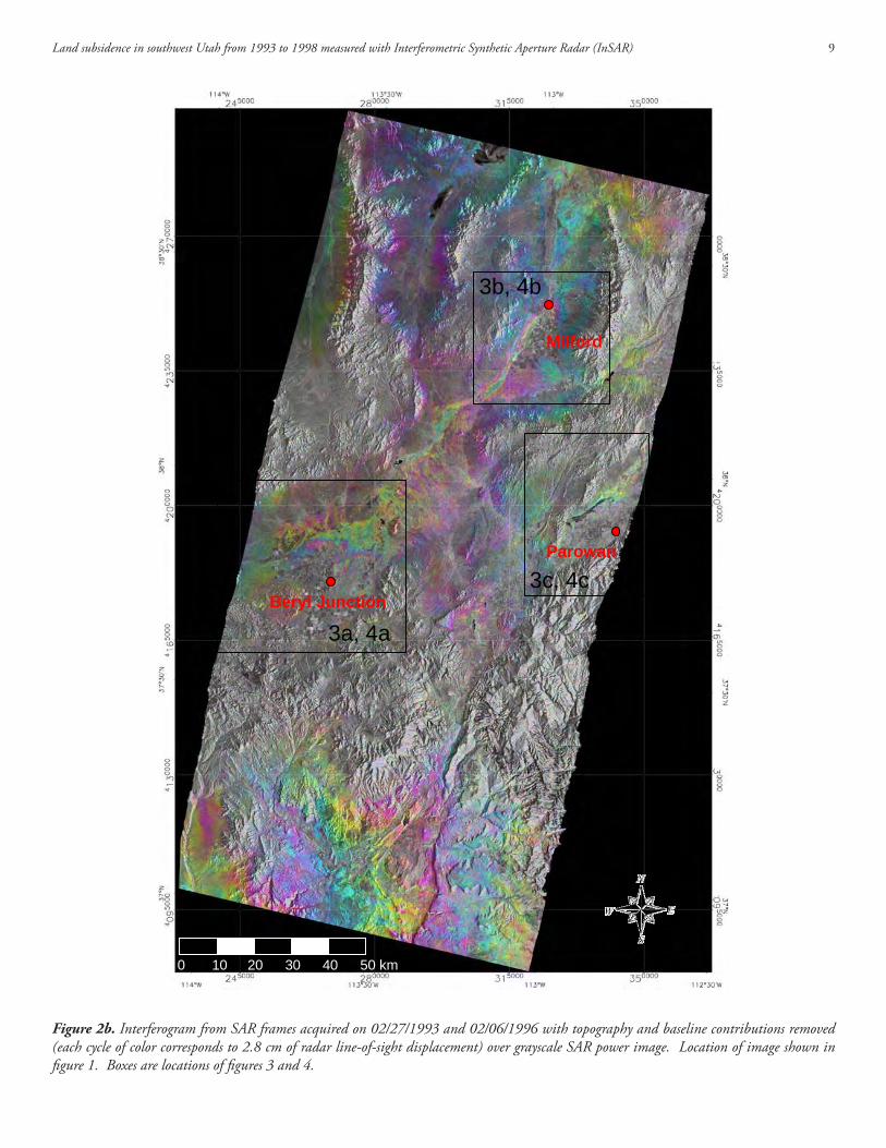
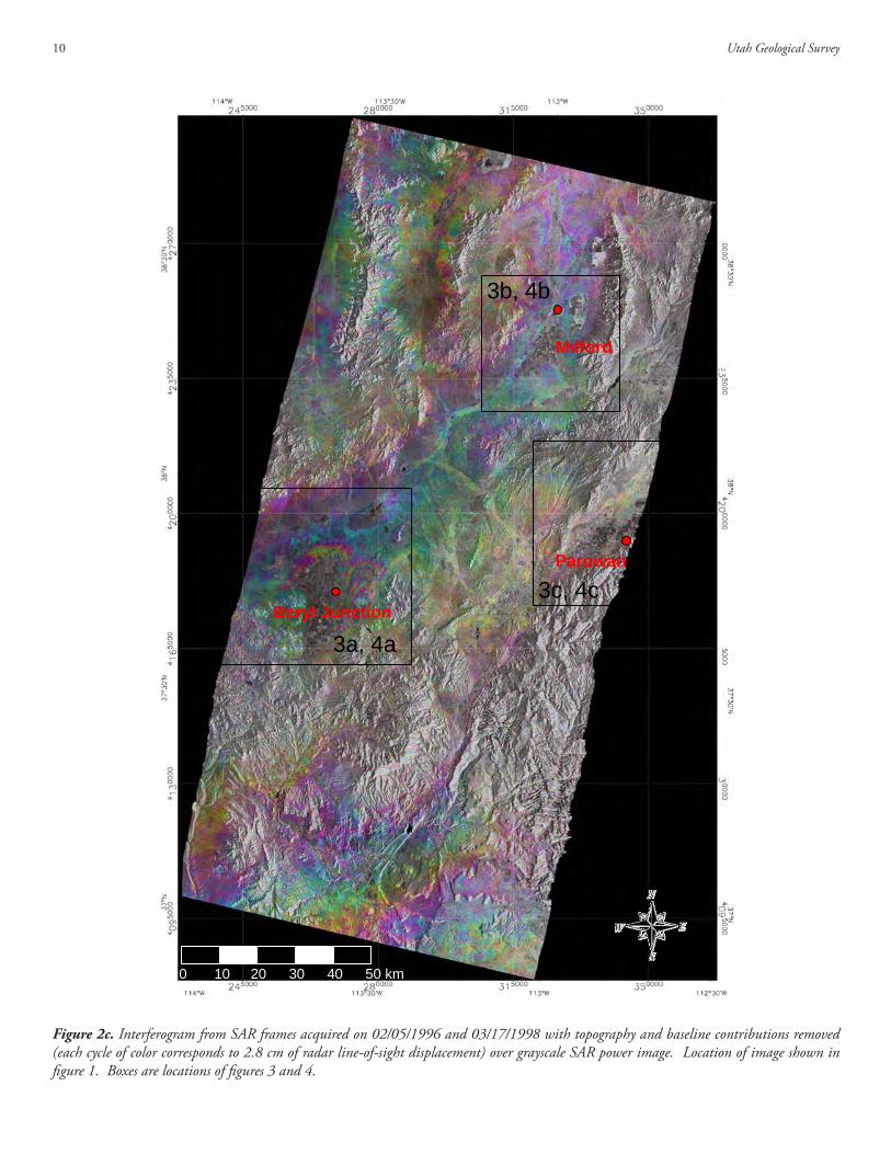
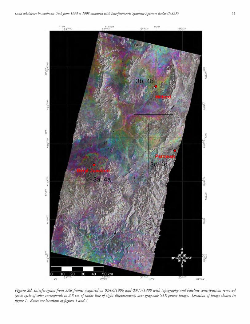
RESULTS AND ANALYSISThe four georeferenced interferograms with the best coherence are shown in figure 2. The color represents the change in phase of the radar signal between the two SAR acquisition dates and the under-lying grayscale is the SAR power image corresponding to the first date of the pair. At this step in the processing, the phase change due to topography and the spatial baseline has been removed. The remaining contributions to the phase are surface motion, changes in the atmosphere or soil moisture, and residual spatial baseline. The atmosphere, soil moisture, and residual baseline are addressed below. These preliminary images are used to assess the presence of surface motion for the three areas of interest (boxes in figure 2). Even at this broad view multiple fringes of color are obvious in the Escalante Valley indicating surface displacement.

The one-day separation between the ERS-1 and ERS-2 acquisi-tions on February 5 and 6, 1996, are useful for separating long-term changes (surface motion over years) from short-term changes (daily atmospheric and soil moisture variation). Each of these

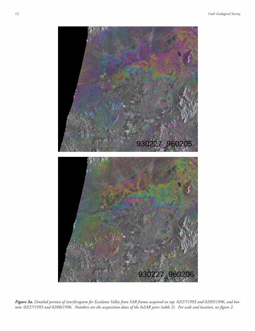
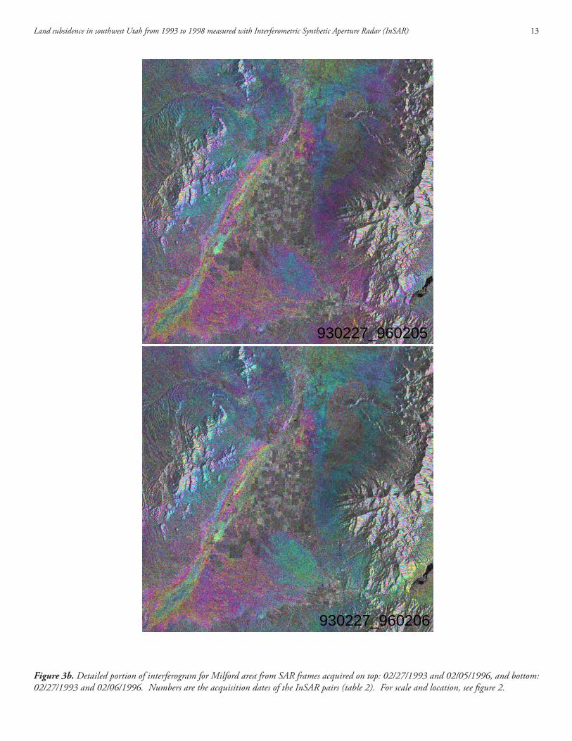
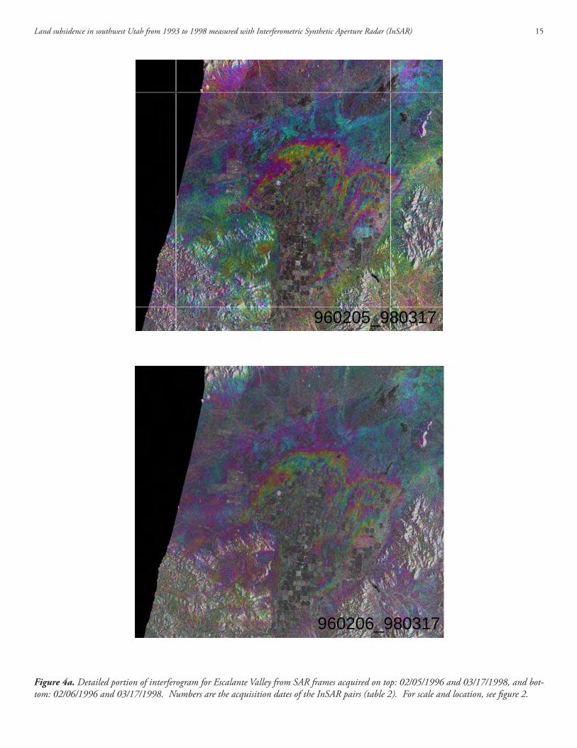
February 1996 scenes is paired with the earlier February 1993 scene to form two similar interferograms. A more detailed view of the three areas of interest is shown in figure 3. The phase pat-tern in the Escalante Valley area is consistent between the 930227-960205 fringe image and the 930227-960206 fringe image (fig-ure 3a). The location of the colors themselves is not the same, as this assignment is arbitrary, but the shape of the color contours is similar. This implies the phase pattern is not due to daily time-scale changes in the atmosphere or soil moisture. The color pat-terns in Milford and Parowan are more subtle and are typically less than one color cycle, nevertheless they are consistent between the 930227-960205 and the 930227-960206 pairs (figures 3a and b). This implies the phase change is likely due to long-term change. This same analysis is applied to the more recent time interval from February 1996 to March 1998 (figure 4). The shape of the color contours is consistent between the two interferograms for all three areas (figure 4a-c) indicating the phase is dominated by long-term change.

It is also useful to make comparisons between the two general time intervals of 1993 to 1996 and 1996 to 1998. The spatial extent of the color is limited by the coherence of the phase signal, which is controlled by the stability of the radar-scattering proper-ties on the ground. Radar scattering can be affected by the surface conditions (e.g. snow cover, soil state, and crop type and density) at the time of SAR acquisition. Therefore it is reasonable to expect slightly different coverage areas for the phase of the two different time periods. with this in mind, a comparison of the phase pat-tern during 1993-1996 is similar to that of 1996-1998 for each of the three areas, especially in Escalante Valley (figures 3a and 4a). This similarity in pattern also indicates the deformation pat-tern has generally been spatially consistent over this time period. Individual results from each of the three study areas are discussed below.

Escalante Valley

A summary of the processing steps from the interferogram stage to the final displacement map is included in this section because it has the strongest deformation signal of the three areas. The interferograms in figure 2 were filtered and unwrapped, convert-ing the cyclical phase from 0 to 360 degrees into an accumulative phase from 0 to 360 multiplied by the number of phase cycles in the image. An adaptive filter that adjusts for the local phase gradient was used to reduce the spatial phase noise. A minimum acceptable coherence value (related to the phase noise) is used to minimize phase unwrapping errors. Unwrapping errors can re-sult in areas with apparent abrupt changes in phase relative to the neighboring area, which, in turn, produce false surface-dis-placement discontinuities. The adaptive filter parameters and the coherence threshold were selected iteratively to exclude obvious areas of phase unwrapping errors. Portions of the interferogram with coherence values below the threshold are not unwrapped and will not have a value in the final displacement map.


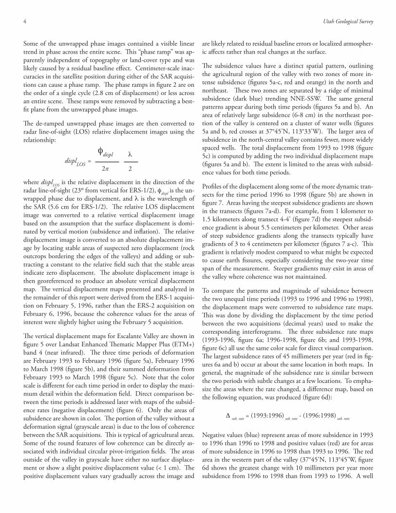
Some of the unwrapped phase images contained a visible linear trend in phase across the entire scene. This “phase ramp” was ap-parently independent of topography or land-cover type and was likely caused by a residual baseline effect. centimeter-scale inac-curacies in the satellite position during either of the SAR acquisi-tions can cause a phase ramp. The phase ramps in figure 2 are on the order of a single cycle (2.8 cm of displacement) or less across an entire scene. These ramps were removed by subtracting a best-fit plane from the unwrapped phase images.

The de-ramped unwrapped phase images are then converted to radar line-of-sight (LoS) relative displacement images using the relationship:

where displLOS is the relative displacement in the direction of the radar line-of-sight (23º from vertical for ERS-1/2), φdispl is the un-wrapped phase due to displacement, and λ is the wavelength of the SAR (5.6 cm for ERS-1/2). The relative LoS displacement image was converted to a relative vertical displacement image based on the assumption that the surface displacement is domi-nated by vertical motion (subsidence and inflation). The relative displacement image is converted to an absolute displacement im-age by locating stable areas of suspected zero displacement (rock outcrops bordering the edges of the valleys) and adding or sub-tracting a constant to the relative field such that the stable areas indicate zero displacement. The absolute displacement image is then georeferenced to produce an absolute vertical displacement map. The vertical displacement maps presented and analyzed in the remainder of this report were derived from the ERS-1 acquisi-tion on February 5, 1996, rather than the ERS-2 acquisition on February 6, 1996, because the coherence values for the areas of interest were slightly higher using the February 5 acquisition.

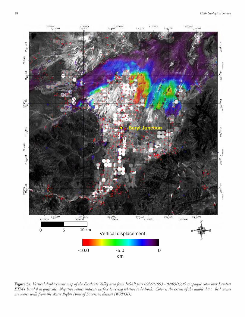
The vertical displacement maps for Escalante Valley are shown in figure 5 over Landsat Enhanced Thematic Mapper Plus (ETM+) band 4 (near infrared). The three time periods of deformation are February 1993 to February 1996 (figure 5a), February 1996 to March 1998 (figure 5b), and their summed deformation from February 1993 to March 1998 (figure 5c). Note that the color scale is different for each time period in order to display the maxi-mum detail within the deformation field. Direct comparison be-tween the time periods is addressed later with maps of the subsid-ence rates (negative displacement) (figure 6). only the areas of subsidence are shown in color. The portion of the valley without a deformation signal (grayscale areas) is due to the loss of coherence between the SAR acquisitions. This is typical of agricultural areas. Some of the round features of low coherence can be directly as-sociated with individual circular pivot-irrigation fields. The areas outside of the valley in grayscale have either no surface displace-ment or show a slight positive displacement value (< 1 cm). The positive displacement values vary gradually across the image and

are likely related to residual baseline errors or localized atmospher-ic affects rather than real changes at the surface.

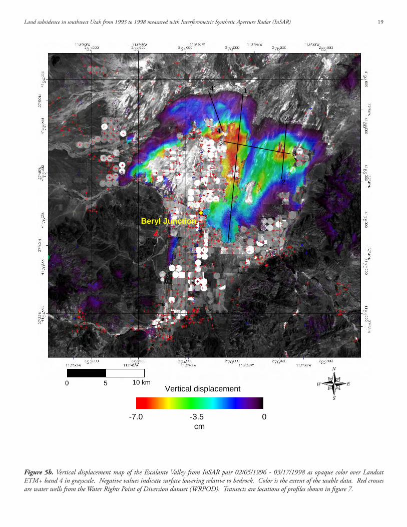
The subsidence values have a distinct spatial pattern, outlining the agricultural region of the valley with two zones of more in-tense subsidence (figures 5a-c, red and orange) in the north and northeast. These two zones are separated by a ridge of minimal subsidence (dark blue) trending NNE-SSw. The same general patterns appear during both time periods (figures 5a and b). An area of relatively large subsidence (6-8 cm) in the northeast por-tion of the valley is centered on a cluster of water wells (figures 5a and b, red crosses at 37°45'N, 113°33'w). The larger area of subsidence in the north-central valley contains fewer, more widely spaced wells. The total displacement from 1993 to 1998 (figure 5c) is computed by adding the two individual displacement maps (figures 5a and b). The extent is limited to the areas with subsid-ence values for both time periods.

Profiles of the displacement along some of the more dynamic tran-sects for the time period 1996 to 1998 (figure 5b) are shown in figure 7. Areas having the steepest subsidence gradients are shown in the transects (figures 7a-d). For example, from 1 kilometer to 1.5 kilometers along transect 4-4' (figure 7d) the steepest subsid-ence gradient is about 5.5 centimeters per kilometer. other areas of steep subsidence gradients along the transects typically have gradients of 3 to 4 centimeters per kilometer (figures 7 a-c). This gradient is relatively modest compared to what might be expected to cause earth fissures, especially considering the two-year time span of the measurement. Steeper gradients may exist in areas of the valley where coherence was not maintained.

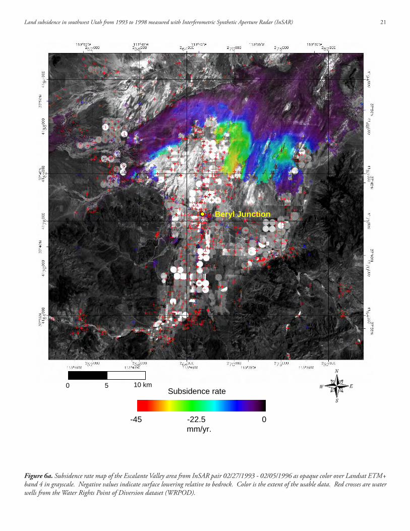
To compare the patterns and magnitude of subsidence between the two unequal time periods (1993 to 1996 and 1996 to 1998), the displacement maps were converted to subsidence rate maps. This was done by dividing the displacement by the time period between the two acquisitions (decimal years) used to make the corresponding interferograms. The three subsidence rate maps (1993-1996, figure 6a; 1996-1998, figure 6b; and 1993-1998, figure 6c) all use the same color scale for direct visual comparison. The largest subsidence rates of 45 millimeters per year (red in fig-ures 6a and b) occur at about the same location in both maps. In general, the magnitude of the subsidence rate is similar between the two periods with subtle changes at a few locations. To empha-size the areas where the rate changed, a difference map, based on the following equation, was produced (figure 6d):

∆ sub. rate = (1993:1996) sub. rate - (1996:1998) sub. rate

Negative values (blue) represent areas of more subsidence in 1993 to 1996 than 1996 to 1998 and positive values (red) are for areas of more subsidence in 1996 to 1998 than 1993 to 1996. The red area in the western part of the valley (37°45'N, 113°45'w, figure 6d shows the greatest change with 10 millimeters per year more subsidence from 1996 to 1998 than from 1993 to 1996. A well

φdispl

2π

λ

2displLOS =


in this area (c-35-17, 14ccc-1; figure 31 in , Burden and others., 2003) shows the same rate of decreasing water level over the time 1993-1996 as 1996-1998 (approximately 2 ft/yr). The blue areas of decreasing subsidence rate are concentrated in the northeast portion of the valley at the southern edge of the data and along the ridge of minimal subsidence. wells with records closest to these areas (c-34-16, 22bad-1 and c-35-15, 6cdd-1; figure 31 in Burden and others., 2003) also have a constant rate of decreasing water level over the time 1993-1996 as 1996-1998, but at slower rates of 1.2 and 1.4 ft/yr, respectively, than in the western part of the area. It is also worth noting that sand dunes have been mapped in the Escalante Valley (Siders, 1985; Siders and others, 1990) and movement of them would likely cause loss of the dis-placement signal from low coherence due to the redistribution of radar scatterers from the repositioning of the sand.

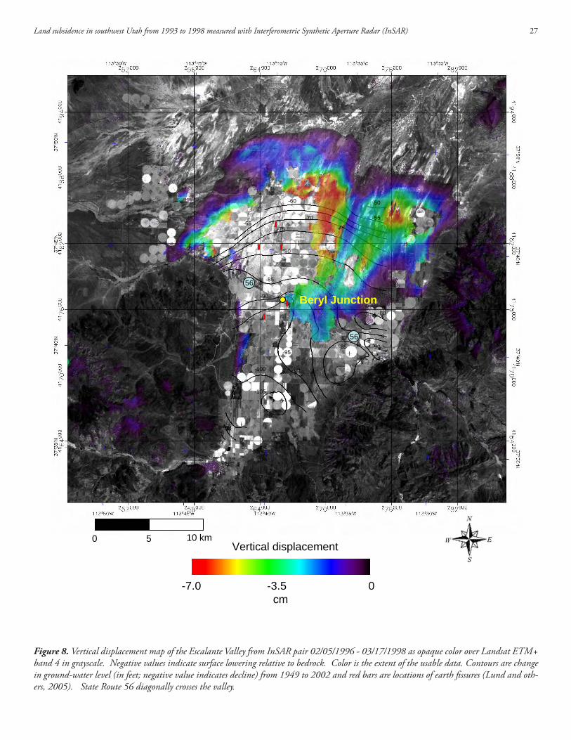
Earth fissures have recently been observed in the Escalante Valley near Beryl Junction. The approximate location of these features along with contours of change in ground-water level from 1949 to 2002 (Lund and others, 2005) are shown with the vertical dis-placement map of 1996 to 1998 (figure 8). This displacement map was selected because it is the most recent time period and has the more extensive coverage. Most of the fissures occur in the central part of the valley where coherence is low and displace-ment measurements could not be made. The one exception is the Beryl Junction fissure near the intersection of SR 56 and the -95 ft contour (figure 8). North and East of the fissure between 2 and 4 centimeters of subsidence occurred between 1996 and 1998 and the gradient in the area is approximately 2.3 centimeters per kilometer. Earth fissures are local features tens of meters to kilometers long, but likely related to regional subsidence (Gallo-way and others, 2004; Lund and others, 2005). Their location is also controlled by basin-fill heterogeneity and depth to basement. Therefore, while the identification of subsidence in an area is an indication of potential for earth fissures it is not the only factor determining their presence or location.

Milford

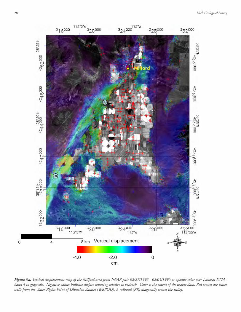
Vertical displacement maps (figure 9) for the Milford area were produced using the same steps described in the Escalante Valley section above. Subsidence has occurred in this area but to a lesser degree than in the Escalante Valley, at least for the regions with good coherence. The diminished subsidence compared to Es-calante Valley is even evident at the interferogram stage. Figures 3b and 4b indicate there is not much more than a single color cycle (fringe) across the Milford area. During the time period 1993 to 1996 the maximum subsidence is 4 cm and it occurs in several lo-cations along the railroad bordering the valley on the west (figure 9a). The largest region of subsidence is centered on the railroad at UTM position 316000E, 4240000N; no wells are located near this area. The other areas of highest subsidence (shown in red) are collocated with water wells (figure 9a).

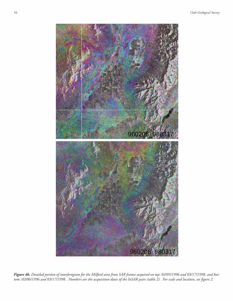
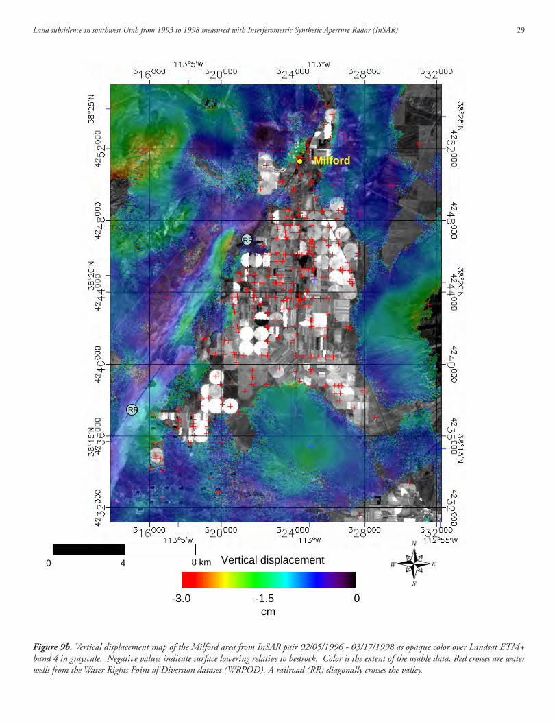
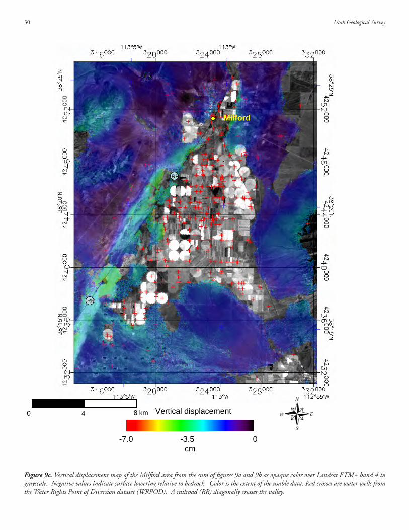
For the period 1996 to 1998 the general pattern of subsidence along the railroad and on the western edge of the valley is similar to the 1993 to 1996 subsidence data. However, the magnitude is decreased by about 25% due to the shorter time span (note the change in color scale for figure 9b). Some changes to the specific locations of the subsidence maxima along the railroad are evident. For example, the two yellow areas on the railroad in 1993-1996 (figure 9a) are replaced by a single yellow area located between the two in the 1996-1998 displacement map (figure 9b). There is also some apparent subsidence (1.5 to 2.5 cm) occurring in two locations in the mountains to the northwest and east of the valley (figure 9b). This is most likely due to atmospheric affects caused by gradients in water vapor content related to topography. The total subsidence from 1993 to 1998 is summed from the two dis-placement maps in figure 9c, range from 0 to 6 centimeters in Milford Valley.

Parowan

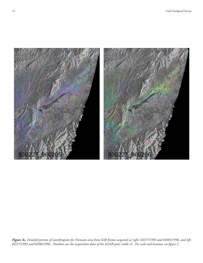
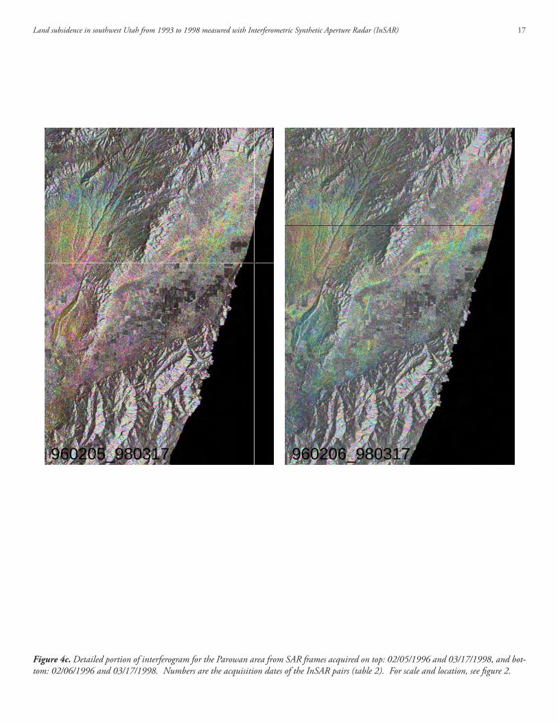
A displacement map for the Parowan Valley could not be pro-duced due to the low-phase coherence that prohibited phase un-wrapping. Numerous combinations of adaptive filter parameters and coherence thresholds were used, but all generated inadequate unwrapped images with either too many gaps or too many un-wrapping errors to form a reliable displacement map. However, a qualitative assessment of surface displacement can be made from the wrapped phase in the interferogram (figures 3c and 4c). From 1993 to 1996 less than a fringe (color cycle) occurs across the val-ley indicating less than 2.8 centimeters of surface change (figure 3c). More color variation exists in the 1996 to 1998 interfero-gram (figure 4c), but not much more than a fringe and the varia-tion is diffuse without much of a phase gradient.

CONCLUSIONS AND RECOMMENDATIONS

Long-term subsidence in southwest Utah is detectable and mea-surable with satellite-based InSAR. of the three regions analyzed the greatest subsidence is in the Escalante Valley. Subsidence rates as high as 3 to 4 centimeters per year were measured approxi-mately 6 kilometers northeast of Beryl Junction from 1993 to 1998 (the most recent usable ERS-2 InSAR data for this area). This is consistent with a recent GPS-based subsidence rate esti-mate of 3 centimeters per year near Beryl Junction for the period 1941 to 1972 (Lund and others, 2005). Increased subsidence may be occurring in the center of the valley but conventional In-SAR measurements are limited to areas of stable radar-scattering properties, which tend to be on the perimeter of the agricultural valleys. Some isolated areas of increased subsidence correspond with locations of water wells. Two zones of subsidence exist in the north and northeast of the valley separated by a prominent


“ridge” of minimal subsidence. For the Escalante Valley the sub-sidence rate is generally consistent between the two time periods measured (1993 to 1996 and 1996 to 1998) with isolated areas of change. The location of one of the earth fissures (“Beryl Junction earth fissure,” Lund and others, 2005) is at the western edge of the InSAR measurements indicating 1.5 centimeters per year of subsidence.

Subsidence in the Milford area is present but with a lower rate (< 1.5 cm/yr) and smaller spatial extent than in the Escalante Valley. The detected subsidence is concentrated on the west side of the valley, adjacent and parallel to the railroad.

The coherence of the radar signal in the Parowan area was too low to produce displacement maps. However, interpretations from preliminary processing steps indicate that any subsidence occur-ring there is probably less intense than that measured in Milford.

More recent and future measurements of subsidence in the Es-calante Valley are possible with InSAR using the ESA’s latest SAR, Envisat. Envisat was launched in 2002 as an upgraded replace-ment for ERS-1 and ERS-2. ESA has archived Envisat scenes of the Escalante Valley area over the time period of 2003 to 2006, which could be used for a more recent assessment of the subsid-ence rate and pattern. To insure that Envisat data are available in the future for this area, it may be necessary to schedule acquisi-tions with ESA. Envisat, like the ERS satellites, repeats its orbit every 35 days. However, data are only acquired by a purchase re-quest from a user. The Escalante Valley area lies within a popular Envisat orbit that has been frequently requested by seismologists because this orbit includes a tectonically active area of southern california. More winter scenes could also be available if acquisi-tions were requested specifically for this Utah subsidence project, which would optimize the spatial extent of the deformation maps over the agricultural fields. Therefore, to insure the appropriate data are available to continue subsidence mapping with InSAR, it is recommended that regular purchases of winter Envisat scenes are initiated now and continue into the future.

The InSAR technique used in this report is the standard approach to deriving a land surface deformation map (e.g. Massonnet and Rabaute, 1993; Rosen and others, 2000). It requires two SAR ac-quisitions, and allows for displacement measurements to be made between the two acquisition dates. However, for the method to work, the radar scattering properties of the surface must remain stable over the entire area of interest. A more recently developed InSAR technique uses a series of SAR scenes (> 10) to generate a time series of surface deformation at individual points. This technique requires minimum points have stable scattering prop-erties. These points, referred to as “persistent scatterers,” act as virtual GPS bench marks which allow for millimeter-scale surface-change measurements over multiple years. Thus, a longer time se-ries of deformation is possible with the persistent scatterer InSAR technique than with the standard InSAR technique. If persistent scatterers can be found in the central portion of an agricultural

area (e.g., near Beryl Junction) this would also allow displacement measurements to be extended spatially into areas where maximum subsidence may be occurring. The persistent scatterer technique could be used on the time series of SAR scenes already acquired by ERS-1 and ERS-2 (1993 – 2004). It could also be used on the Envisat time series as long as acquisitions over the areas of interest are continued into the future.

ACkNOwLEDGMENTSFunding for this study was provided by the Utah Geological Sur-vey. The SAR data were purchased from Eurimage.

REFERENCESBurden and others., 2003, Ground-water conditions in Utah,

Spring of 2003, cooperative Investigations Report No. 44: Utah Department of Natural Resources, Division of water Resources, 120 p.

Forster, R., 2005, Investigation of the potential of interferometric synthetic aperture radar (InSAR) to detect land subsidence in Sw Utah: Utah Geological Survey open-File Report 446, 21p.

Delft, 2005, web page, http://www.deos.tudelft.nl/ers/precorbs/

Lund, w.R., DuRoss c.B., kirby S.M., McDonald G.N., Hunt G., and Vice, G.S., 2005, The origin and extent of earth fis-sures in Escalante Valley, Southern Escalante Desert, Iron county, Utah: Utah Geological Survey Special Study 115, 29p.

Massonnet, D., and Rabaute, T., 1993, Radar interferometry – Limits and potential, IEEE Trans. on Geos. and Rem. Sens., 31, 455-464.

Rosen, P. A., Hensley, S., Joughin, I. R., Li, F. k., Madsen, S. N., Rodriguez, E., and Goldstein, R., 2000, Synthetic aperture radar interferometry, Proceedings of the IEEE, 88, 333-382.

Siders, M.A., Rowley, P.D., Shubat, M.A., christenson, G.c., and Galyardt, G.L., 1990, Geologic map of the Newcastle quadrangle, Iron county, Utah: U.S. Geological Survey Map GQ-1690, scale 1:24,000.

Siders, M.A., 1985, Geologic map of the Beryl Junction quadran-gle, Iron county, Utah: Utah Geological and Mineral Survey Map 85, scale 1:24,000.


Figure 1. Southwest corner of Utah with blue boxes indicating approximate location of the two SAR frames listed in Table 1. Inset map (http://gazetteer.hometownlocator.com), Base map (U.S. Geological Survey, Reston, VA, 1989.)

0 10 20 30 40 50 km

Beryl Junction

Milford

Parowan

Figure 1. Southwest corner of Utah with blue boxes indicating approximate location of the two SAR frames listed in table 1. Inset map (http://gazetteer.hometownlocator.com), base map (U.S. Geological Survey, Reston, VA, 1989).


Figure 2a. Interferogram from SAR frames acquired on 02/27/1993 and 02/05/1996 with topography and baseline contributions removed (each cycle of color corresponds to 2.8 cm of radar line-of-sight displacement) over gray-scale SAR power image. Location of image shown in Figure 1. Boxes are locations of Figures and 3 and 4.

3a, 4a

3c, 4c

3b, 4b

Beryl Junction

Milford

Parowan

0 10 20 30 40 50 km

Figure 2a. Interferogram from SAR frames acquired on 02/27/1993 and 02/05/1996 with topography and baseline contributions removed (each cycle of color corresponds to 2.8 cm of radar line-of-sight displacement) over grayscale SAR power image. Location of image shown in figure 1. Boxes are locations of figures 3 and 4.


Figure 2b. Interferogram from SAR frames acquired on 02/27/1993 and 02/06/1996 with topography and baseline contributions removed (each cycle of color corresponds to 2.8 cm of radar line-of-sight displacement) over grayscale SAR power image. Location of image shown in figure 1. Boxes are locations of figures 3 and 4.

3a, 4a

3c, 4c

3b, 4b

Beryl Junction

Milford

Parowan

0 10 20 30 40 50 km

Figure 2b. Interferogram from SAR frames acquired on 02/27/1993 and 02/06/1996 with topography and baseline contributions removed (each cycle of color corresponds to 2.8 cm of radar line-of-sight displacement) over gray-scale SAR power image. Location of image shown in Figure 1. Boxes are locations of Figures and 3 and 4.


Figure 2c. Interferogram from SAR frames acquired on 02/05/1996 and 03/17/1998 with topography and baseline contributions removed (each cycle of color corresponds to 2.8 cm of radar line-of-sight displacement) over grayscale SAR power image. Location of image shown in figure 1. Boxes are locations of figures 3 and 4.

3a, 4a

3c, 4c

3b, 4b

Beryl Junction

Milford

Parowan

0 10 20 30 40 50 km

Figure 2c. Interferogram from SAR frames acquired on 02/05/1996 and 03/17/1998 with topography and baseline contributions removed (each cycle of color corresponds to 2.8 cm of radar line-of-sight displacement) over gray-scale SAR power image. Location of image shown in Figure 1. Boxes are locations of Figures and 3 and 4.


Figure 2d. Interferogram from SAR frames acquired on 02/06/1996 and 03/17/1998 with topography and baseline contributions removed (each cycle of color corresponds to 2.8 cm of radar line-of-sight displacement) over grayscale SAR power image. Location of image shown in figure 1. Boxes are locations of figures 3 and 4.

3a, 4a

3c, 4c

3b, 4b

Beryl Junction

Milford

Parowan

0 10 20 30 40 50 km

Figure 2d. Interferogram from SAR frames acquired on 02/06/1996 and 03/17/1998 with topography and baseline contributions removed (each cycle of color corresponds to 2.8 cm of radar line-of-sight displacement) over gray-scale SAR power image. Location of image shown in Figure 1. Boxes are locations of Figures and 3 and 4.


930227_960205

930227_960206

Figure 3a. Detailed portion of interferogram for Escalante Valley from SAR frames acquired on top: 02/27/1993 and 02/05/1996, and bottom: 02/27/1993 and 02/06/1996. Numbers are the acquisition dates of the InSAR pairs (Table 2). For scale and location see figure 2.

Figure 3a. Detailed portion of interferogram for Escalante Valley from SAR frames acquired on top: 02/27/1993 and 02/05/1996, and bot-tom: 02/27/1993 and 02/06/1996. Numbers are the acquisition dates of the InSAR pairs (table 2). For scale and location, see figure 2.


Figure 3b. Detailed portion of interferogram for Milford area from SAR frames acquired on top: 02/27/1993 and 02/05/1996, and bottom: 02/27/1993 and 02/06/1996. Numbers are the acquisition dates of the InSAR pairs (table 2). For scale and location, see figure 2.

Figure 3b. Detailed portion of interferogram for Milford area from SAR frames acquired on top: 02/27/1993 and 02/05/1996, and bottom: 02/27/1993 and 02/06/1996. Numbers are the acquisition dates of the InSAR pairs (Table 2). For scale and location see figure 2.

930227_960205

930227_960206


Figure 3c. Detailed portion of interferogram for Parowan area from SAR frames acquired at right: 02/27/1993 and 02/05/1996, and left: 02/27/1993 and 02/06/1996. Numbers are the acquisition dates of the InSAR pairs (table 2). For scale and location, see figure 2.

Figure 3c. Detailed portion of interferogram for Parowan area from SAR frames acquired at right: 02/27/1993 and 02/05/1996, and left: 02/27/1993 and 02/06/1996. Numbers are the acquisition dates of the InSAR pairs (Table 2). For scale and location see figure 2.

930227_960205 930227_960206


Figure 4a. Detailed portion of interferogram for Escalante Valley from SAR frames acquired on top: 02/05/1996 and 03/17/1998, and bottom: 02/06/1996 and 03/17/1998. Numbers are the acquisition dates of the InSAR pairs (Table 2). For scale and location see figure 2.

960205_980317

960206_980317

Figure 4a. Detailed portion of interferogram for Escalante Valley from SAR frames acquired on top: 02/05/1996 and 03/17/1998, and bot-tom: 02/06/1996 and 03/17/1998. Numbers are the acquisition dates of the InSAR pairs (table 2). For scale and location, see figure 2.


Figure 4b. Detailed portion of interferogram for the Milford area from SAR frames acquired on top: 02/05/1996 and 03/17/1998, and bot-tom: 02/06/1996 and 03/17/1998. Numbers are the acquisition dates of the InSAR pairs (table 2). For scale and location, see figure 2.

Figure 4b. Detailed portion of interferogram for the Milford area from SAR frames acquired on top: 02/05/1996 and 03/17/1998, and bottom: 02/06/1996 and 03/17/1998. Numbers are the acquisition dates of the InSAR pairs (Table 2). For scale and location see figure 2.

960205_980317

960206_980317


Figure 4c. Detailed portion of interferogram for the Parowan area from SAR frames acquired on top: 02/05/1996 and 03/17/1998, and bot-tom: 02/06/1996 and 03/17/1998. Numbers are the acquisition dates of the InSAR pairs (table 2). For scale and location, see figure 2.

Figure 4c. Detailed portion of interferogram for the Parowan area from SAR frames acquired on top: 02/05/1996 and 03/17/1998, and bottom: 02/06/1996 and 03/17/1998. Numbers are the acquisition dates of the InSAR pairs (Table 2). For scale and location see figure 2.

960205_980317 960206_980317


-10.0 -5.0 0cm

Vertical displacement

Figure 5a. Vertical displacement map of the Escalante Valley area from InSAR pair 02/27/1993 -02/05/1996 as opaque color over Landsat ETM+ band 4 in gray-scale. Negative values indicate surface lowering relative to bedrock. Color is the extent of the usable data. Red crosses are water wells from the Water Rights Point of Diversion dataset (WRPOD).

0 5 10 km

Beryl Junction

Figure 5a. Vertical displacement map of the Escalante Valley area from InSAR pair 02/27/1993 - 02/05/1996 as opaque color over Landsat ETM+ band 4 in grayscale. Negative values indicate surface lowering relative to bedrock. Color is the extent of the usable data. Red crosses are water wells from the Water Rights Point of Diversion dataset (WRPOD).


Figure 5b. Vertical displacement map of the Escalante Valley from InSAR pair 02/05/1996 - 03/17/1998 as opaque color over Landsat ETM+ band 4 in grayscale. Negative values indicate surface lowering relative to bedrock. Color is the extent of the usable data. Red crosses are water wells from the Water Rights Point of Diversion dataset (WRPOD). Transects are locations of profiles shown in figure 7.

-7.0 -3.5 0cm


Figure 5b. Vertical displacement map of the Escalante Valley from InSAR pair 02/05/1996 – 03/17/1998 as opaque color over Landsat ETM+ band 4 in gray-scale. Negative values indicate surface lowering relative to bedrock. Color is the extent of the usable data. Red crosses are water wells from the Water Rights Point of Diversion dataset (WRPOD). Transects are locations of profiles shown in Figure 7.

1

1’

3’

3

2’

2

4’

4

0 5 10 km

Beryl Junction


Figure 5c. Vertical displacement map of the Escalante Valley from the sum of figures 5a and 5b as opaque color over Landsat ETM+ band 4 in grayscale. Negative values indicate surface lowering relative to bedrock. Color is the extent of the usable data. Red crosses are water wells from the Water Rights Point of Diversion dataset (WRPOD).

-17.0 -8.5 0cm


Figure 5c. Vertical displacement map of the Escalante Valley from the sum of figures 5a and 5b as opaque color over Landsat ETM+ band 4 in gray-scale. Negative values indicate surface lowering relative to bedrock. Color is the extent of the usable data. Red crosses are water wells from the Water Rights Point of Diversion dataset (WRPOD).

0 5 10 km

Beryl Junction


-45 -22.5 0mm/yr.

Subsidence rate0 5 10 km

Beryl Junction

Figure 6a. Subsidence rate map of the Escalante Valley area from InSAR pair 02/27/1993 - 02/05/1996 as opaque color over Landsat ETM+ band 4 in gray-scale. Negative values indicate surface lowering relative to bedrock. Color is the extent of the usable data. Red crosses are water wells from the Water Rights Point of Diversion dataset (WRPOD). Figure 6a. Subsidence rate map of the Escalante Valley area from InSAR pair 02/27/1993 - 02/05/1996 as opaque color over Landsat ETM+

band 4 in grayscale. Negative values indicate surface lowering relative to bedrock. Color is the extent of the usable data. Red crosses are water wells from the Water Rights Point of Diversion dataset (WRPOD).


Figure 6b. Subsidence rate map of the Escalante Valley area from InSAR pair 02/05/1996 - 03/17/1998 as opaque color over Landsat ETM+ band 4 in grayscale. Negative values indicate surface lowering relative to bedrock. Color is the extent of the usable data. Red crosses are water wells from the Water Rights Point of Diversion dataset (WRPOD).

-45 -22.5 0mm/yr.


Beryl Junction

Figure 6b. Subsidence rate map of the Escalante Valley area from InSAR pair 02/05/1996 - 03/17/1998 as opaque color over Landsat ETM+ band 4 in gray-scale. Negative values indicate surface lowering relative to bedrock. Color is the extent of the usable data. Red crosses are water wells from the Water Rights Point of Diversion dataset (WRPOD).


Figure 6c. Subsidence rate map of the Escalante Valley area from the sum of figures 6a and 6b as opaque color over Landsat ETM+ band 4 in grayscale. Negative values indicate surface lowering relative to bedrock. Color is the extent of the usable data. Red crosses are water wells from the Water Rights Point of Diversion dataset (WRPOD).

-45 -22.5 0mm/yr.


Beryl Junction

Figure 6c. Subsidence rate map of the Escalante Valley area from the sum of figures 6a and 6b as opaquecolor over Landsat ETM+ band 4 in gray-scale. Negative values indicate surface lowering relative to bedrock. Color is the extent of the usable data. Red crosses are water wells from the Water Rights Point of Diversion dataset (WRPOD).


Figure 6d. Change in subsidence rate of the Beryl Junction area from the difference of figures 6a and 6b as opaque color over Landsat ETM+ band 4 in grayscale. Negative values (blue) represent areas where there was more subsidence in 1993 to 1996 than 1996 to 1998 and positive values (red) are for areas where there was more subsidence in 1996 to 1998 than 1993 to 1996. Red crosses are water wells from the Water Rights Point of Diversion dataset (WRPOD).

Figure 6d. Change in subsidence rate of the Beryl Junction area from the difference of figures 6a and 6b as opaque color over Landsat ETM+ band 4 in gray-scale. Negative values (blue) represent areas where there was more subsidence in 1993 to 1996 than 1996 to 1998 and positive values (red) are for areas where there was more subsidence in 1996 to 1998 than 1993 to 1996. Red crosses are water wells from the Water Rights Point of Diversion dataset (WRPOD).

-10 0 10mm/yr.

Change in subsidence rate0 5 10 km

Beryl Junction


-8

-7

-6

-5

-4

-3

-2

-1

0

1

0 2 4 6 8 10 12 14 16 18 20

Distance (km)

Verti

cal s

urfa

ce d

ispl

acem

ent (

cm)

South North

Figure 7a. Profile of vertical displacement from 02/05/1996 to 03/17/1998 along transect 1-1’ in Figure 5b.

-8

-7

-6

-5

-4

-3

-2

-1

0

1

0 1 2 3 4 5 6 7

Distance (km)

Verti

cal s

urfa

ce d

ispl

acem

ent (

cm)

South North

Figure 7b. Profile of vertical displacement from 02/05/1996 to 03/17/1998 along transect 2-2’ in Figure 5b.

-8

-7

-6

-5

-4

-3

-2

-1

0

1

0 2 4 6 8 10 12 14 16 18 20

Distance (km)

Verti

cal s

urfa

ce d

ispl

acem

ent (

cm)

South North

Figure 7a. Profile of vertical displacement from 02/05/1996 to 03/17/1998 along transect 1-1’ in Figure 5b.

-8

-7

-6

-5

-4

-3

-2

-1

0

1

0 1 2 3 4 5 6 7

Distance (km)

Verti

cal s

urfa

ce d

ispl

acem

ent (

cm)

South North

Figure 7b. Profile of vertical displacement from 02/05/1996 to 03/17/1998 along transect 2-2’ in Figure 5b.

Figure 7a. Profile of vertical displacement from 02/05/1996 to 03/17/1998 along transect 1-1' in figure 5b.

Figure 7b. Profile of vertical displacement from 02/05/1996 to 03/17/1998 along transect 2-2' in figure 5b.


Figure 7c. Profile of vertical displacement from 02/05/1996 to 03/17/1998 along transect 3-3' in figure 5b.

Figure 7d. Profile of vertical displacement from 02/05/1996 to 03/17/1998 along transect 4-4' in figure 5b.

-8

-7

-6

-5

-4

-3

-2

-1

0

0 1 2 3 4 5 6 7 8 9

Distance (km)

Verti

cal s

urfa

ce d

ispl

acem

ent (

cm)

West East

Figure 7c. Profile of vertical displacement from 02/05/1996 to 03/17/1998 along transect 3-3’ in Figure 5b.

-8

-7

-6

-5

-4

-3

-2

-1

0

1

0 0.5 1 1.5 2 2.5 3 3.5 4 4.5 5

Distance (km)

Verti

cal s

urfa

ce d

ispl

acem

ent (

cm)

South North

Figure 7d. Profile of vertical displacement from 02/05/1996 to 03/17/1998 along transect 4-4’ in Figure 5b.

-8

-7

-6

-5

-4

-3

-2

-1

0

0 1 2 3 4 5 6 7 8 9

Distance (km)

Verti

cal s

urfa

ce d

ispl

acem

ent (

cm)

West East

Figure 7c. Profile of vertical displacement from 02/05/1996 to 03/17/1998 along transect 3-3’ in Figure 5b.

-8

-7

-6

-5

-4

-3

-2

-1

0

1

0 0.5 1 1.5 2 2.5 3 3.5 4 4.5 5

Distance (km)

Verti

cal s

urfa

ce d

ispl

acem

ent (

cm)

South North

Figure 7d. Profile of vertical displacement from 02/05/1996 to 03/17/1998 along transect 4-4’ in Figure 5b.


-7.0 -3.5 0cm


Figure 8. Vertical displacement map of the Escalante Valley from InSAR pair 02/05/1996-03/17/1998 as opaque color over Landsat ETM+ band 4 in gray-scale. Negative values indicate surface lowering relative to bedrock. Color is the extent of the usable data. Contours are change in ground-water level (in feet; negative value indicates decline) from 1949 to 2002 and red bars are locations of earth fissures (Lund and others, 2005). State Route 56 is labeled diagonally crossing the valley.

-50

-55

-60

-65-70

-75

-80

-85

-90

-95

-80

-85 -90

-100

-105

0 5 10 km

Beryl Junction56

56

Figure 8. Vertical displacement map of the Escalante Valley from InSAR pair 02/05/1996 - 03/17/1998 as opaque color over Landsat ETM+ band 4 in grayscale. Negative values indicate surface lowering relative to bedrock. Color is the extent of the usable data. Contours are change in ground-water level (in feet; negative value indicates decline) from 1949 to 2002 and red bars are locations of earth fissures (Lund and oth-ers, 2005). State Route 56 diagonally crosses the valley.


-4.0 -2.0 0cm


Figure 9a. Vertical displacement map of the Milford area from InSAR pair 02/27/1993 - 02/05/1996 as opaque color over Landsat ETM+ band 4 in gray-scale. Negative values indicate surface lowering relative to bedrock. Color is the extent of the usable data. Red crosses are water wells from the Water Rights Point of Diversion dataset (WRPOD). A railroad is labeled diagonally crossing the valley.

0 4 8 km

Milford

RR

RR

Figure 9a. Vertical displacement map of the Milford area from InSAR pair 02/27/1993 - 02/05/1996 as opaque color over Landsat ETM+ band 4 in grayscale. Negative values indicate surface lowering relative to bedrock. Color is the extent of the usable data. Red crosses are water wells from the Water Rights Point of Diversion dataset (WRPOD). A railroad (RR) diagonally crosses the valley.


Figure 9b. Vertical displacement map of the Milford area from InSAR pair 02/05/1996 - 03/17/1998 as opaque color over Landsat ETM+ band 4 in grayscale. Negative values indicate surface lowering relative to bedrock. Color is the extent of the usable data. Red crosses are water wells from the Water Rights Point of Diversion dataset (WRPOD). A railroad (RR) diagonally crosses the valley.

Figure 9b. Vertical displacement map of the Milford area from InSAR pair 02/05/1996 – 03/17/1998 as opaque color over Landsat ETM+ band 4 in gray-scale. Negative values indicate surface lowering relative to bedrock. Color is the extent of the usable data. Red crosses are water wells from the Water Rights Point of Diversion dataset (WRPOD). A railroad is labeled diagonally crossing the valley.

-3.0 -1.5 0cm

Vertical displacement0 4 8 km

Milford

RR

RR


Figure 9c. Vertical displacement map of the Milford area from the sum of figures 9a and 9b as opaque color over Landsat ETM+ band 4 in grayscale. Negative values indicate surface lowering relative to bedrock. Color is the extent of the usable data. Red crosses are water wells from the Water Rights Point of Diversion dataset (WRPOD). A railroad (RR) diagonally crosses the valley.

Figure 9c. Vertical displacement map of the Milford area from the sum of figures 9a and 9b as opaque color over Landsat ETM+ band 4 in gray-scale. Negative values indicate surface lowering relative to bedrock. Color is the extent of the usable data. Red crosses are water wells from the Water Rights Point of Diversion dataset (WRPOD). A railroad is labeled diagonally crossing the valley.

-7.0 -3.5 0cm

Vertical displacement0 4 8 km

Milford

RR

RR

insar - utah subsidence in southwest utah from 1993 to 1998 measured with interferometric synthetic...

Documents