a finite-element approach to predict permanent deformation

A Finite-Element Approach to Predict PermanentDeformation Behaviour of Hot Mix Asphalt Basedon Fundamental Material Tests and AdvancedRheological Models

R. Blab*, K. Kappl*, E. Aigner† and R. Lackner‡

*Institute for Road Construction & Maintenance, Vienna University of Technology, Vienna, Austria†Institute for Mechanics of Materials and Structures, Vienna University of Technology, Vienna, Austria‡Material-Technology Unit, University of Innsbruck, Technikerstraße 13, 6020 Innsbruck, Austria

ABSTRACT: An ongoing research project, undertaken at the Christian Doppler Laboratory for

‘performance-based optimisation of flexible road pavements’, focuses on the evaluation of advanced

rheological models (i.e. Power Law, Huet and Huet–Sayegh) to describe permanent deformation

behaviour of hot mix asphalt (HMA) and their implementation in a finite-element (FE) code. To

accomplish this, an appropriate algorithm was developed for the summation of the different con-

tributions of the stress history to determine the resulting creep strain tensor to simulate real-life

stress/strain situations in flexible road pavements. Furthermore, the mathematical background for

parameter identification from dynamic stiffness tests (four-point bending beam and dynamic tension

compression tests) has been developed and a straightforward programme for data fitting is pre-

sented. For the validation of the implemented constitutive equations derived for the selected rhe-

ological models, a FE simulation of triaxial tests on cylindrical HMA specimens was carried out.

KEY WORDS: advanced non-linear viscoelastic rheological models, finite-element-modelling

Introduction

The calculation of displacements, stresses or strains in

the different layers of flexible pavements (hot mixed

asphalt materials), caused by vehicle loads, is a simple

task when linear elastic material behaviour is consid-

ered. However, in reality surface, base course and

granular layers show a more complex constitutive

behaviour, with nonlinear and time-dependent effects

(viscoelastic and viscoplastic material behaviour).

Decades ago, researchers have found that the defor-

mation of asphalt concrete AC under load is composed

of reversible viscoelastic (VE) and irreversible visco-

plastic (VP) components [e.g. 1–4]. Since then, con-

stitutive equations are constantly under development.

Aside from obeying laws, they must describe the

behaviour of the material accurately under different

loading and temperature conditions.

In the last decade, important achievements in the

development of improved rheological models that

describe the complex behaviour of AC have been

made. For example, Schapery model [5], which

includes a linear VE model with damage and a sepa-

rate VP model, was chosen by the National Cooper-

ative Highway Research Programme (NCHRP 9-19)

research team for modelling AC behaviour [6]. At

increasing straining, the observed stiffness reduction

is modelled through the damage caused by the

material. The formulation was extended to three

dimensional 3D conditions by Uzan and Levenberg

[7]. Studies by Di Benedetto et al. [8] allowed the

formulation of a general 1D linear viscoelastic model

with a continuum spectrum called 2S2P1D, two

springs, two parabolic elements, one dashpot. It has

been shown, that the 2S2P1D model is powerful to

determine the linear viscoelastic behaviour in the

small strain domain of bituminous binders, mastics

and mixes, over a very wide range of frequencies and

temperatures. Recently, this model developed to

simulate the 1D thermo-elasto-viscoplastic behaviour

of bituminous materials was formulated for the 3D

case in the linear range [9]. Another material model

adopted by the Delft University uses the flow surface

proposed by Desai et al. [10] in combination with a

set of constitutive relations developed to facilitate

the description of asphalt concrete response [11].

Such material models could be used in mechanistic

pavement design methodologies, which consider

pavement structural response to predict specific distress

and failure modes. Today, there is a trend to substitute

� 2009 The Authors. Journal compilation � 2009 Blackwell Publishing Ltd j Strain (2009) 45, 3–16 3

pavement analysis based on the Multilayer Elastic

Theory by analysis based on finite-element methods

(FEM). A pre-requisite for the use of the FEM is the

availabilityofmaterialmodels thatontheonehandcan

describe the triaxial behaviour in both the linear and

nonlinear range and offers straightforward algorithms

to solve the constitutive equations in an acceptable

computational time period. While on the other hand

and even more important the used model should

reduce the costly experimental laboratory work needed

for material parameter identification to a minimum.

The objective of this work was to identify such

suitable rheological models, which then were imple-

mented in a finite-element (FE) code to enable the

simulation of real-life stress/strain situations in flex-

ible road pavements. Hereby, an appropriate

algorithm was developed for the summation of the

different contributions of the stress history to deter-

mine the resulting creep strain tensor. The mathe-

matical background for parameter identification

from cyclic stiffness tests according to EN 12697-26

[12] was implemented in work sheets for easy data

fitting. In a last step, the performance of the selected

rheological models was evaluated by FE simulation of

permanent deformations, appearing in triaxial tests

on cylindrical specimens made of the two conven-

tional hot mix asphalt (HMA) base course materials.

Tested Materials

Within the research work various surface course and

base course asphalt materials were tested, whereas in

this paper only two base course materials (AC22 base

50/70 and AC22 bin PmB45/80-65) are presented.

The first one is a conventional base course asphalt

concrete material with a maximum aggregate size of

32 mm and a conventional binder 70/100, the sec-

ond material is an asphalt concrete material with the

same sieve curve but a high modified binder PmB45/

80-65. The aggregate that was used the asphalt mixes

was a limestone called ‘Hollitzer’. The main data of

the mixes can be seen in Table 1 and Figures 1–5. The

grading curves of the AC22 base used for the both AC

types are illustrated in Figure 1.

Figure 2 shows the Cole–Cole representations

(elastic vs. viscous parts of the dynamic modulus E**)

and Figure 3 shows the black diagrams (dynamic

modulus E** vs. phase lag U) for both, the 50/70 and

PmB 45/80-65, binders derived from uniaxial cyclic

stiffness tests on prismatic specimen (DTC-PR;

length l · width w · height h ¼ �60 · 60 · 200

mm3) according to EN 12697-26 [12]. The Cole–Cole

and black diagrams for the asphalt mixtures AC 22

base 50/70 and AC 22 bin PmB45/80-65, are shown in

Figures 4 and 5.

Selected Rheological Models and TheirMathematical Background

Selected rheological models

Rheological models, which relate the applied stress

history to the accumulated viscoelastic strains, take

the viscoelastic material response of asphalt into

account. Over the last decades, a large number of

material models for the description of the viscoelastic

Table 1: Main characteristics of base course materials AC22 base 50/70 and AC22 bin PmB45/80-65

Characteristic Unit EN Standard

AC22 base

50/70

AC22bin

PmB45/80-65

Type of binder – EN 12591 and prEN 14023 50/70 PmB 45/80-65

Penetration 1/10 mm EN 1426 56.3 77.5

Softening point R&B �C EN 1427 50.3 68.2

Bending beam rheometer m-value ()18 �C) – EN 14771 0.325 0.388

Bending beam rheometer S-value ()18 �C) MPa EN 14771 284 110

Dynamic shear rheometer dynamic

shear modulus G* (+46 �C)

MPa EN 14770 23 950 18 258

Dynamic shear rheometer phase lag U (+46 �C) degrees EN 14770 79.6 62.3

Rotational viscosimeter RV (+135 �C) MPa s EN 13302 492.8 1439.9

Binder content mass% – 4.5 4.5

Aggregate density qa (limestone) Mg m)3 EN 1097-6 2.850 2.850

Maximum density asphalt qR Mg m)3 EN 12697-5 2.612 2.612

bulk density asphalt specimen qSSD Mg m)3 EN 12697-6 2.484 2.499

Air void content V vol% EN 12697-6 4.9 4.3

Marshall stability kN EN 12697-34 11.2 13.3

Marshall flow mm EN 12697-34 3.0 3.9

4 � 2009 The Authors. Journal compilation � 2009 Blackwell Publishing Ltd j Strain (2009) 45, 3–16

AFE Approach to Predict Permanent Deformation Behaviour : R. Blab et al.

behaviour of asphalt were developed, starting with

simple rheological models such as the Maxwell or

Kelvin–Voigt model, which can be represented by

one spring and one linear dashpot [13]. With these

models, it is not possible to fit the experimentally

observed nonlinearity in the creep deformations

properly. Consequently other, more complex rheo-

logical models were developed, consisting of non-

linear (parabolic) dashpots that model the observed

nonlinearity [1, 2, 8]. These models are, i.e. the Power

Law model, represented by a linear spring and a

parabolic dashpot in series, or the Huet model, con-

sisting of a linear spring with two nonlinear dashpots

in series. Table 2 gives an overview about all rheo-

logical models considered in this paper. Whereas the

Huet model is well suited for the description of

monotonic loading of asphalt, it is not really suitable

for predicting the behaviour under cyclic loading. As

a remedy, the Huet–Sayegh model, obtained from

adding a linear spring in parallel to the Huet model,

was employed.

Based on the strain history under constant loading,

three regimes of creep are commonly distinguished:

primary, secondary and tertiary creep. The different

creep regimes are distinguished mathematically by

the time derivative of the creep strain rate, d2e/dt2,

under constant loading, with d2e/dt2 < 0 for primary

creep, d2e/dt2 ¼ 0 for secondary creep and d2e/dt2 > 0

for tertiary creep. Hereby, the shift from primary to

secondary and, finally, from secondary to tertiary

creep is explained by the opening of microcracks and

the formation of plastic failure zones in the material

0

1020

30

4050

60

70

8090

100

0.01 0.1 1 10 100Sieve size (mm)

Pass

ing

% (

m-%

)AC22 base 50/70

Figure 1: Grading curve AC22 base 50/70

0102030405060708090

E* (MPa)

Phi (

°)

Phi (

°)

+46°C+40°C+34°C+28°C+22°C+16°C–20°C

0102030405060708090

0.001 0.01 0.1 1 10 0.001 0.01 0.1 1 10

E* (MPa)

+46°C+40°C+34°C+28°C+22°C+16°C+10°C+4°C–8°C–14°C–20°C

Figure 3: Black diagrams (dynamic modulus E* vs. phase lag U) of conventional binder 50/70 (left side) and modified binder

PmB 45/80-65 (right side)

0

0.5

1

1.5

0 1 2 3 4 5

E1 (MPa)

E2

(MPa

) +46 °C+40 °C+34 °C+28 °C+22 °C+16 °C–20 °C

0

0.5

1

1.5

0 1 2 3 4 5

E1 (MPa)

E2

(MP

a) +46 °C+40 °C+34 °C+28 °C+22 °C+16 °C+10 °C+4 °C–8 °C–14 °C–20 °C

Figure 2: Cole–Cole representations (elastic part E1 and viscous part E2 of dynamic modulus E*) of conventional binder 50/70

(left side) and modified binder PmB 45/80-65 (right side)

0

1000

2000

3000

4000

5000

0 10 000 20 000 30 000 40 000

E1 (MPa)

E2

(MPa

)

E2

(MPa

) –10 °C 0 °C +10 °C +20 °C

0

1000

2000

3000

4000

5000

0 10 000 20 000 30 000 40 000

E1 (MPa)

–10 °C0 °C +10 °C +20 °C

Figure 4: Black diagrams (dynamic modulus E* vs. phase lag U) and Cole–Cole representations (elastic part E1 and viscous part

E2 of dynamic modulus E*) of conventional base course material AC22 base 50/70 (left side) and modified base course material AC22

bin PmB 45/80-65 (right side)


R. Blab et al. : AFE Approach to Predict Permanent Deformation Behaviour

microstructure leading to the collapse of the mate-

rial. To capture the entire creep response of the

material (from primary creep to material failure),

nonlinear creep laws, relating the applied stress to

the creep strain in a nonlinear manner, were pro-

posed in the open literature, reading e ¼ Jrn with J

denoting the creep compliance and n > 1. For mod-

erate loading situations, which do not cause cracking

and the formation of plastic zones, creep deforma-

tions remain in the primary creep regime and linear

creep laws, characterised by n ¼ 1, can be used to

describe the material response.

In the case of linear creep, any nonlinearity

observed in the creep deformation response is cap-

tured by the compliance function J. This function

was determined for different viscoelastic material

models (see Table 2). Whereas J is obtained by a

simple summation of contributions for models

characterised by a serial arrangement of springs and

dashpots, parallel arrangement results in internal

stress redistribution even in case of constant external

loading. In case of the Kelvin–Voigt model, i.e. the

underlying differential equation describing this

redistribution can be solved analytically, giving an

explicit expression for the creep compliance func-

tion. For the Huet–Sayegh model, on the other hand,

a numerical solution algorithm was developed. An

analytical expression for the Huet–Sayegh compli-

ance function for arbitrary values for h and k does not

exist [14].

Mathematical backgrounds

The following chapter gives a brief overview of the

mathematical backgrounds for the rheological mod-

els presented here (Power Law model, Huet model

and Huet–Sayegh model).

Power Law modelThe Power Law model is an extension of Maxwell’s

very basic model. It consists of a linear elastic spring

and a parabolic (nonlinear) dashpot connected in

series. Because of this serial connection, the static

creep compliance J(t) used to describe tests with static

loading can be obtained by adding up the creep

compliances Ji(t) of the two elements (spring and

dashpot):

JPLðtÞ ¼ JSP þ JPDPðtÞ ¼ 1

E1þ Ja

t

s

� �k

(1)

Hereby, JSP (1/MPa) stands for the creep compli-

ance of the spring and JPDP (1/MPa) for the creep

compliance of the parabolic dashpot. E¥ (MPa) is the

stiffness of the spring, Ja the creep compliance at t ¼s, where s (s) is the characteristic time of the under-

lying viscous process. k represents a dimensionless

parameter influencing the behaviour of the dashpot

with time.

To obtain the dynamic compliance out of this

Equation (1), the following relationship is needed:

Table 2: Creep compliance functions J

(MPa)1) for different rheological modelsRheological model Creep function J(t) Parameters

Power-Law-Model E Ja , k , 1

( )k

a

tJ t J

EE , Ja, k,

Huet modelE Ja , k , Jb , h , 1

( )k h

a b

t tJ t J J

EE , Ja, Jb, k, h,

Huet-Sayegh modelE Ja , k , Jb , h ,

E0

numerically solved E0, E , Ja, Jb, k, h,

0102030405060708090

100 1000 10 000 100 000

E* (MPa)

Phi (

°) –10 °C0 °C+10 °C+20 °C

0102030405060708090

100 1000 10 000 100 000

E* (MPa)

Phi (

°) –10°C0°C+10°C+20°C

Figure 5: Black diagrams (dynamic modulus E* vs. phase lag U) of conventional base course material AC22 base 50/70 (left side)

and modified base course material AC22 bin PmB 45/80-65 (right side)



J�ðxÞ¼ ixZ 1

0

Jðn0Þe�ixn0 dn0 ¼ ðixÞL½Jðn0Þ�s¼ix¼ðixÞJðixÞ

(2)

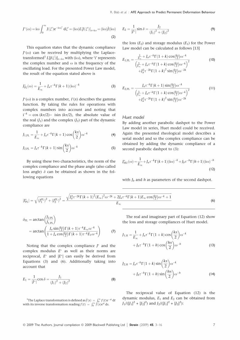
This equation states that the dynamic compliance

J�(x) can be received by multiplying the Laplace-

transformed1 L[J(n¢)]s¼ix with (ix), where ‘i’ represents

the complex number and x is the frequency of the

oscillating load. For the presented Power Law model,

the result of the equation stated above is

J�PLðxÞ ¼1

E1þ Jas

�kCðkþ 1ÞðixÞ�k(3)

J�(x) is a complex number, C(x) describes the gamma

function. By taking the rules for operations with

complex numbers into account and noting that

i)k ¼ cos (kp/2)) isin (kp/2), the absolute value of

the real (J1) and the complex (J2) part of the dynamic

compliance are

J1;PL ¼1

E1þ Jas

�kCðkþ 1Þ coskp2

� �x�k (4)

J2;PL ¼ Jas�kCðkþ 1Þ sin kp

2

� �x�k (5)

By using these two characteristics, the norm of the

complex compliance and the phase angle (also called

loss angle) d can be obtained as shown in the fol-

lowing equations

dPL ¼ arctanJ2;PL

J1;PL

� �

¼ arctanJa sin kp

2

� �Cðkþ 1Þs�kE1x�k

1þ Ja cos kp2

� �Cðkþ 1Þs�kE1x�k

!(7)

Noting that the complex compliance J� and the

complex modulus E� as well as their norms are

reciprocal, E� and |E�| can easily be derived from

Equations (3) and (6). Additionally taking into

account that

E1 ¼1

jJ�j cos d ¼ J1

ðJ1Þ2 þ ðJ2Þ2(8)

E2 ¼1

jJ�j sin d ¼ J2

ðJ1Þ2 þ ðJ2Þ2(9)

the loss (E2) and storage modulus (E1) for the Power

Law model can be calculated as follows [13]

E1;PL ¼1

E1þ Jas�kCð1þ kÞ cos kp

2

� �x�k

1E1þ Jas�kCð1þ kÞ cos kp

2

� �x�k

� �2

þJ2a s�2kCð1þ kÞ2 sin kp

2

� �x�2k

(10)

E2;PL ¼Jas�kCðkþ 1Þ sin kp

2

� �x�k


2

� �x�k

� �2

þJ2a s�2kCð1þ kÞ2 sin kp

2

� �x�2k

(11)

Huet modelBy adding another parabolic dashpot to the Power

Law model in series, Huet model could be received.

Again the presented rheological model describes a

serial model and so the complex compliance can be

obtained by adding the dynamic compliance of a

second parabolic dashpot to (3):

J�HUðxÞ¼1

E1þ Jas

�kCðkþ1ÞðixÞ�kþ Jbs�hCðhþ1ÞðixÞ�h

(12)

with Jb and h as parameters of the second dashpot.

The real and imaginary part of Equation (12) show

the loss and storage compliances of Huet model.

J1;H ¼1

E1þ Jas

�kCð1þ kÞ coskp2

� �x�k

þ Jbs�hCð1þ hÞ cos

hp2

� �x�h (13)

J2;H ¼ Jas�kCð1þ kÞ sin kp

2

� �x�k

þ Jbs�hCð1þ hÞ sin hp

2

� �x�h (14)

The reciprocal value of Equation (12) is the

dynamic modulus, E1 and E2 can be obtained from

J1/([J1]2 + [J2]2) and J2/([J1]2 + [J2]2):

jJ�PLj ¼ffiffiffiffiffiffiffiffiffiffiffiffiffiffiffiffiffiffiffiffiffiffiffiffiffiffiffiffiffiffiðJPL

1 Þ2 þ ðJPL

2 Þ2

q¼

ffiffiffiffiffiffiffiffiffiffiffiffiffiffiffiffiffiffiffiffiffiffiffiffiffiffiffiffiffiffiffiffiffiffiffiffiffiffiffiffiffiffiffiffiffiffiffiffiffiffiffiffiffiffiffiffiffiffiffiffiffiffiffiffiffiffiffiffiffiffiffiffiffiffiffiffiffiffiffiffiffiffiffiffiffiffiffiffiffiffiffiffiffiffiffiffiffiffiffiffiffiffiffiffiffiffiffiffiffiffiffiffiffiffiffiffiffiffiffiffiffiffiffiffiffiffiffiffiffiffiffiJ2a s�2kCðkþ 1Þ2ðE1Þ2x�2k þ 2Jas�kCðkþ 1ÞE1 cos kp

2

� �x�k þ 1

qE1

(6)

1The Laplace transformation is defined as f ðsÞ ¼R1

0 f ðtÞe�st dt

with its inverse transformation reading f ðtÞ ¼R1

0 f ðsÞest ds.



E1;H ¼


2

� �x�k

þJbs�hCð1þ hÞ cos hp2

� �x�h

DEN(15)

E2;H ¼Jas�kCð1þkÞsin kp

2

� �x�kþ Jbs�hCð1þhÞsin hp

2

� �x�h

DEN(16)

whereas the denominator DEN is

DEN ¼ 1

E1þ Jas

�kCð1þ kÞ coskp2

� �x�k

�

þJbs�hCð1þ hÞ cos

hp2

� �x�h

�2

þ Jas�kCð1þ kÞ sin kp

2

� �x�k

�

þJbs�hCð1þ hÞ sin hp

2

� �x�h

�2

(17)

The phase angle d could be calculated from

E2,H/E1,H and J2,H/J1,H respectively [13].

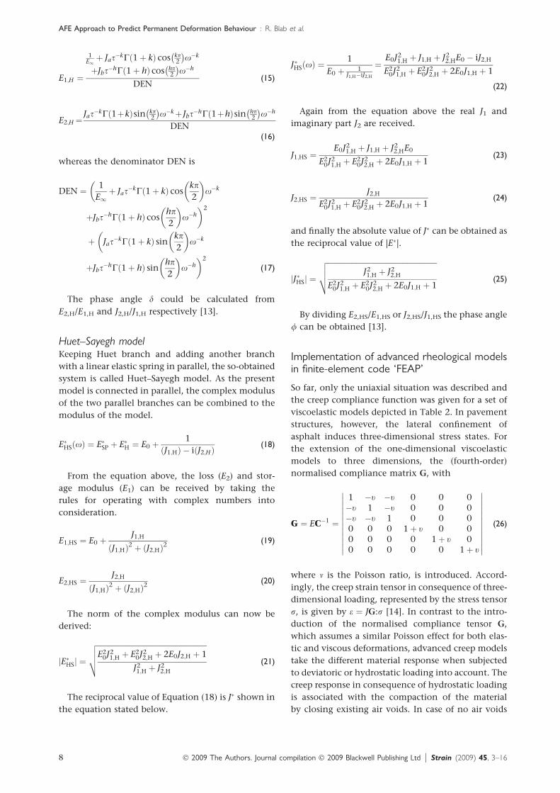
Huet–Sayegh modelKeeping Huet branch and adding another branch

with a linear elastic spring in parallel, the so-obtained

system is called Huet–Sayegh model. As the present

model is connected in parallel, the complex modulus

of the two parallel branches can be combined to the

modulus of the model.

E�HSðxÞ ¼ E�SP þ E�H ¼ E0 þ1

ðJ1;HÞ � iðJ2;HÞ(18)

From the equation above, the loss (E2) and stor-

age modulus (E1) can be received by taking the

rules for operating with complex numbers into

consideration.

E1;HS ¼ E0 þJ1;H

ðJ1;HÞ2 þ ðJ2;HÞ2(19)

E2;HS ¼J2;H

ðJ1;HÞ2 þ ðJ2;HÞ2(20)

The norm of the complex modulus can now be

derived:

jE�HSj ¼

ffiffiffiffiffiffiffiffiffiffiffiffiffiffiffiffiffiffiffiffiffiffiffiffiffiffiffiffiffiffiffiffiffiffiffiffiffiffiffiffiffiffiffiffiffiffiffiffiffiffiffiffiffiffiffiffiffiffiffiffiE2

0J21;H þ E2

0J22;H þ 2E0J2;H þ 1

J21;H þ J2

2;H

vuut (21)

The reciprocal value of Equation (18) is J� shown in

the equation stated below.

J�HSðxÞ ¼1

E0 þ 1J1;H�iJ2;H

¼E0J2

1;H þ J1;H þ J22;HE0 � iJ2;H

E20J2

1;H þ E20J2

2;H þ 2E0J1;H þ 1

(22)

Again from the equation above the real J1 and

imaginary part J2 are received.

J1;HS ¼E0J2

1;H þ J1;H þ J22;HE0

E20J2

1;H þ E20J2

2;H þ 2E0J1;H þ 1(23)

J2;HS ¼J2;H

E20J2

1;H þ E20J2

2;H þ 2E0J1;H þ 1(24)

and finally the absolute value of J� can be obtained as

the reciprocal value of |E�|.

jJ�HSj ¼

ffiffiffiffiffiffiffiffiffiffiffiffiffiffiffiffiffiffiffiffiffiffiffiffiffiffiffiffiffiffiffiffiffiffiffiffiffiffiffiffiffiffiffiffiffiffiffiffiffiffiffiffiffiffiffiffiffiffiffiffiJ21;H þ J2

2;H

E20J2

1;H þ E20J2

2;H þ 2E0J1;H þ 1

vuut (25)

By dividing E2,HS/E1,HS or J2,HS/J1,HS the phase angle

/ can be obtained [13].

Implementation of advanced rheological modelsin finite-element code ‘FEAP’

So far, only the uniaxial situation was described and

the creep compliance function was given for a set of

viscoelastic models depicted in Table 2. In pavement

structures, however, the lateral confinement of

asphalt induces three-dimensional stress states. For

the extension of the one-dimensional viscoelastic

models to three dimensions, the (fourth-order)

normalised compliance matrix G, with

G ¼ EC�1 ¼

1 �t �t 0 0 0�t 1 �t 0 0 0�t �t 1 0 0 00 0 0 1þ t 0 00 0 0 0 1þ t 00 0 0 0 0 1þ t

(26)

where m is the Poisson ratio, is introduced. Accord-

ingly, the creep strain tensor in consequence of three-

dimensional loading, represented by the stress tensor

r, is given by e ¼ JG:r [14]. In contrast to the intro-

duction of the normalised compliance tensor G,

which assumes a similar Poisson effect for both elas-

tic and viscous deformations, advanced creep models

take the different material response when subjected

to deviatoric or hydrostatic loading into account. The

creep response in consequence of hydrostatic loading

is associated with the compaction of the material

by closing existing air voids. In case of no air voids



(e.g. when considering bitumen or mastic only), no

volumetric creep is observed. As regards the creep

response under deviatoric stress states, no air voids

are required. The deformation results from sliding

effects within the material. In general, the deviatoric

creep response is significantly larger than the creep

deformations associated with hydrostatic loading.

Moreover, the latter is bounded by the air voids

present in the material, while ‘deviatoric’ creep

evolves over longer time scales. To account for

the different material response when subjected

to hydrostatic and deviatoric loading, two creep

compliance functions, one associated with hydro-

static and one associated with deviatoric loading,

may be introduced. Accordingly, the viscoelastic

strain tensor is composed of two contributions,

reading

e ¼ evol þ edev ¼ ½JvolIvol þ JdevIdev� : r; (27)

where Jvol and Jdev are creep compliance functions

describing volumetric and deviatoric creep deforma-

tions associated with hydrostatic and deviatoric stress

states respectively. In the above given equation for

the viscoelastic strain tensor, Ivol and Idev are defined

as [14]

Ivol ¼

1=3 1=3 1=3 0 0 0

1=3 1=3 1=3 0 0 0

1=3 1=3 1=3 0 0 0

0 0 0 0 0 0

0 0 0 0 0 0

0 0 0 0 0 0

and

Idev ¼

2=3 �1=3 �1=3 0 0 0

�1=3 2=3 �1=3 0 0 0

�1=3 �1=3 2=3 0 0 0

0 0 0 1 0 0

0 0 0 0 1 0

0 0 0 0 0 1

(28)

In general, Jvol and Jdev correspond to different

viscoelastic models. As creep under hydrostatic

loading is associated with the closure of air voids in

the material, asymptotic model such as the Kelvin–

Voigt model are well suited to describe volumetric

creep. Under deviatoric loading, on the other hand,

any one of the viscoelastic models shown in Table 2

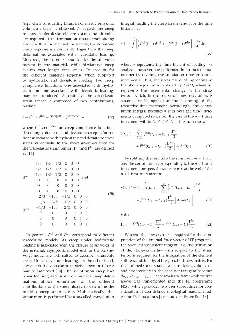
may be employed [14]. The use of linear creep laws

when focusing exclusively on primary creep defor-

mations allows summation of the different

contributions to the stress history to determine the

resulting creep strain tensor. Mathematically, this

summation is performed by a so-called convolution

integral, reading the creep strain tensor for the time

instant t as

eðtÞ ¼Zt

0

1

3Jvolðt � sÞIvol þ 1

2Jdevðt � sÞIdev

�:drds

ds

(29)

where s represents the time instant of loading. FE

analyses, however, are performed in an incremental

manner by dividing the simulation time into time

increments. Thus, the stress rate dr/ds appearing in

the above equation is replaced by Dr/Dt, where Dr

represents the incremental change in the stress

tensor, which, in the course of time integration, is

assumed to be applied at the beginning of the

respective time increment. Accordingly, the convo-

lution integral becomes a sum over the time incre-

ments computed so far. For the case of the n + 1 time

increment within tn £ t £ tn+1, this sum reads:

eðtnþ1Þ ¼Xnþ1

m¼1

hJvolðtnþ1 � tm�1Þ

Ivol

3

þ Jdevðtnþ1 � tm�1ÞIdev

2

i� DrðtmÞ (30)

By splitting the sum into the sum from m ¼ 1 to n

and the contribution corresponding to the n + 1 time

increment, one gets the stress tensor at the end of the

n + 1 time increment as

rðtnþ1Þ ¼ Jnþ1

"eðtnþ1Þ �

Xn

m¼1

hJvolðtnþ1 � tm�1Þ

Ivol

3

þ Jdevðtnþ1 � tm�1ÞIdev

2

i� DrðtmÞ

#(31)

with

Jnþ1 ¼ Jvolðtnþ1 � tnÞIvol

3þ Jdevðtnþ1 � tnÞ

Idev

2(32)

Whereas the stress tensor is required for the com-

putation of the internal force vector of FE programs,

the so-called ‘consistent tangent’, i.e. the derivation

of the stress–strain law with respect to the strain

tensor is required for the integration of the element

stiffness and, finally, of the global stiffness matrix. For

the outlined stress–strain law, considering volumetric

and deviatoric creep, the consistent tangent becomes

drn+1/den+1 ¼ Jn+1. The viscoelastic framework outline

above was implemented into the FE programme

FEAP, which provides two user subroutines for con-

sideration of user-defined rheological material mod-

els for FE simulations [for more details see Ref. 14].



Determination of Material Data andData Fitting

Direct tension and compression stiffness tests

The basis for fitting the various parameters for the

different rheological models are complex modulus

values obtained from dynamic stiffness tests

according to European Standard EN 12697-26

[12]. In this research project, four-point bending

beam tests (4PB-PR) on prismatic specimens

(l · w · h � 500 · 50 · 50 mm3) and direct tension

and compression tests (DTC-CY) on cylindrical

specimen (Ø � 50 mm, h � 200 mm) as well as

on prismatic specimen (DTC-PR; l · w · h ¼�60 · 60 · 200 mm3), both with cyclic sinusoidal

loading were conducted. In this paper, only DTC-

PR test data were used for data fitting and FE sim-

ulation.

In the DTC-PR, a sinusoidal strain e ¼ e0 sin (xt) is

applied on a cylindrical sample glued to two steel

plates screwed to the loading rig. e0 is 25 · 10)6

microstrains (�0.005 mm for a 200-mm-long speci-

men) to avoid specimen damaging. The test tem-

peratures were )10, 0, 10, 20 �C, the frequencies

changed from 0.1 up to 40 Hz (0.1, 1, 2, 5, 10, 15,

20, 30 and 40 Hz). With the measured axial force F,

the axial deformation z and phase angle d the

complex modulus E* could be calculated at different

temperatures and frequencies with the following

equations

E1 ¼h

b1b2

F

zcosðdÞ þ

M2 þm� �

103x2

� �(33)

E2 ¼h

b1b2

F

zsinðdÞ

� �(34)

E� ¼ffiffiffiffiffiffiffiffiffiffiffiffiffiffiffiffiE2

1 þ E22

q(35)

U ¼ arctanE2

E1

� �(36)

where E1 is the real component (MPa), E2 the imagi-

nary component of the complex modulus E* (MPa), F

the measured axial force (N), z the measured axial

deformation (mm), d the measured phase lag (de-

grees), h the specimen height (mm), b1 the width of

specimen (mm), b2 the depth of specimen (mm), M

the mass of specimen (kg), m the mass of movable

test machine parts (kg) and U the calculated material

phase lag without system influences (degrees).

Data fitting procedure

Starting with the measured data (force F, displacement

z and phase angle d) from the DTC-PR stiffness tests at

different temperatures (T ¼ )10, 0, +10, +20 �C) and

frequencies, the storage and loss modulus can be

computed by taking shape and mass factors for the

underlying stiffness test into account. The Cole–Cole

and black diagrams are obtained by plotting E2 against

E1 and U against |E�| respectively – see Figures 3 and 4.

The analytical curve of the selected model can now be

approximated to the data from the tests, if the model’s

parameters – e.g. E0, E¥, Ja, Jb, k and h for Huet–Sayegh

model – by means of curve fitting facilitating the mean

square error method. Figure 6 shows all model fits for

the AC22 bin PmB 45/80-65 material in the Cole–Cole

and black representation and Table 3 summarises all

model parameters for both materials. In this case, the

quality of the fitting, i.e. how well the analytical curve

fits to test data, is increased by minimising the square

error between data and curve in y direction. Hereby,

an analytical characterisation of the materials’

mechanical behaviour is achievable and so obtained

parameters can be used for, e.g. computer-based FE

simulation.

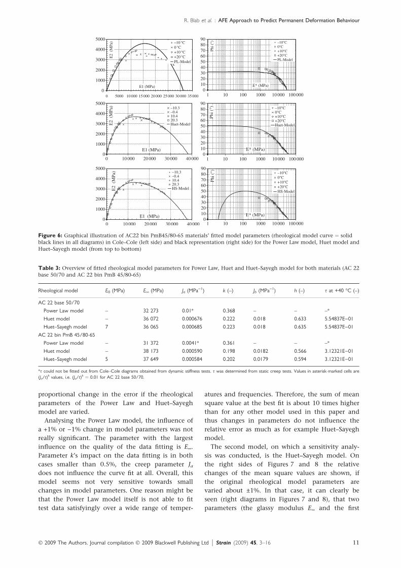
Figure 6 shows, that Huet–Sayegh model results in

the best fit quality, represented by the smallest error

deviation. It is important to note, that the complex

modulus E0 from Huet–Sayegh model has important

influence on the results of FE simulations. Especially,

the phase lag U, shown in the black representations,

decreases enormously with changing E0 values (see

last row, right diagram in Figure 6). The characteristic

creep time s is fitted by using the Arrhenius law

according to Equation (31):

s ¼ 1

s0exp �Ea

R

1

T� 1

T0

� � �(37)

Sensitivity test of models’ parameters anderror analysis

After fitting the test data of any material, tested in

the stiffness tests according to EN 12797-26, it

becomes apparent that an optimum of rheological

model parameters (e.g. E0, E¥, Ja, Jb, k and h) are

existing, for which the sum of the mean square value

is a minimum. Not every rheological parameter has

the same influence on the quality of the data fit. To

find out which parameter has the largest influence

on the behaviour of the model’s analytical curve,

each model parameter was varied by ±1% of the

optimum values by keeping an eye on the behaviour

of the error’s change. Figures 7 and 8 show the



proportional change in the error if the rheological

parameters of the Power Law and Huet–Sayegh

model are varied.

Analysing the Power Law model, the influence of

a +1% or )1% change in model parameters was not

really significant. The parameter with the largest

influence on the quality of the data fitting is E¥.

Parameter k’s impact on the data fitting is in both

cases smaller than 0.5%, the creep parameter Jadoes not influence the curve fit at all. Overall, this

model seems not very sensitive towards small

changes in model parameters. One reason might be

that the Power Law model itself is not able to fit

test data satisfyingly over a wide range of temper-

atures and frequencies. Therefore, the sum of mean

square value at the best fit is about 10 times higher

than for any other model used in this paper and

thus changes in parameters do not influence the

relative error as much as for example Huet–Sayegh

model.

The second model, on which a sensitivity analy-

sis was conducted, is the Huet–Sayegh model. On

the right sides of Figures 7 and 8 the relative

changes of the mean square values are shown, if

the original rheological model parameters are

varied about ±1%. In that case, it can clearly be

seen (right diagrams in Figures 7 and 8), that two

parameters (the glassy modulus E¥ and the first

Table 3: Overview of fitted rheological model parameters for Power Law, Huet and Huet–Sayegh model for both materials (AC 22

base 50/70 and AC 22 bin PmB 45/80-65)

Rheological model E0 (MPa) E¥ (MPa) Ja (MPa)1) k (–) Jb (MPa)1) h (–) s at +40 �C (–)

AC 22 base 50/70

Power Law model – 32 273 0.01* 0.368 – – –*

Huet model – 36 072 0.000676 0.222 0.018 0.633 5.54837E)01

Huet–Sayegh model 7 36 065 0.000685 0.223 0.018 0.635 5.54837E)01

AC 22 bin PmB 45/80-65

Power Law model – 31 372 0.0041* 0.361 – – –*

Huet model – 38 173 0.000590 0.198 0.0182 0.566 3.12321E)01

Huet–Sayegh model 5 37 649 0.000584 0.202 0.0179 0.594 3.12321E)01

*s could not be fitted out from Cole–Cole diagrams obtained from dynamic stiffness tests. s was determined from static creep tests. Values in asterisk-marked cells are

(Ja/t)k values, i.e. (Ja/t)k ¼ 0.01 for AC 22 base 50/70.

0

1000

2000

3000

4000

5000

0 5000 10 000 15 000 20 000 25 000 30 000 35 000

–10 °C 0 °C +10 °C +20 °C PL-Model

E2

(M

Pa)

E1 (MPa) 0

10 20 30 40 50 60 70 80 90

1 10 100 1000 10 000 100 000

–10°C0° C +1 0° C +2 0° C PL-Model

Phi

(°)

E* (MPa)

0

1000

2000

3000

4000

5000

0 10 000 20 000 30 000 40 000

–10.3 –0.4 10.4 20.3 Huet-Model E

2 (

MPa

)

E1 (MPa) 0

10 20 30 40 50 60 70 80 90

1 10 100 1000 10 000 100 000

–10°C 0°C +10°C +20°C Huet-Model

Phi

(°)

E* (MPa)

0

1000

2000

3000

4000

5000

0 10 000 20 000 30 000 40 000

–10.3 –0.4 10.4 20.3 HS-Model E

2 (

MP

a)

E1 (MPa) 0

10 20 30 40 50 60 70 80 90

1 10 100 1000 10 000 100 000

–10°C 0°C +10°C +20°C HS-Model

Phi (

°)

E* (MPa)

Figure 6: Graphical illustration of AC22 bin PmB45/80-65 materials’ fitted model parameters (rheological model curve ¼ solid

black lines in all diagrams) in Cole–Cole (left side) and black representation (right side) for the Power Law model, Huet model and

Huet–Sayegh model (from top to bottom)



dashpot’s exponent k) have a mentionable influ-

ence on the quality of the data fits. E¥ can be

described as the glassy modulus and is important

for the material’s behaviour at low temperatures

and high frequencies. The exponent k physically

specifies the velocity of the viscous model parts at

which deformations increase from the point of the

glassy modulus E¥ (where the viscous modulus

values are zero) if temperatures increase or

frequencies decrease. Increasing values for k mean

increasing permanent deformations if temperature

gets higher and/or frequency gets lower. All other

model parameters have less influence on the mean

square value’s change, as can be seen in Figure 7

and Figure 8. Consequently, the fitting of E¥ and k

have to be carried out most carefully.

Model Validation by Finite-ElementSimulations

Numerical study of triaxial cyclic compressiontests (TCCT) with FE simulation

For validation of the constitutive material presenta-

tions implemented in the FE code the rheological

models are used to simulate the behaviour of asphalt

in triaxial cyclic compression tests (TCCT) on cylin-

drical specimens, according to European Standard EN

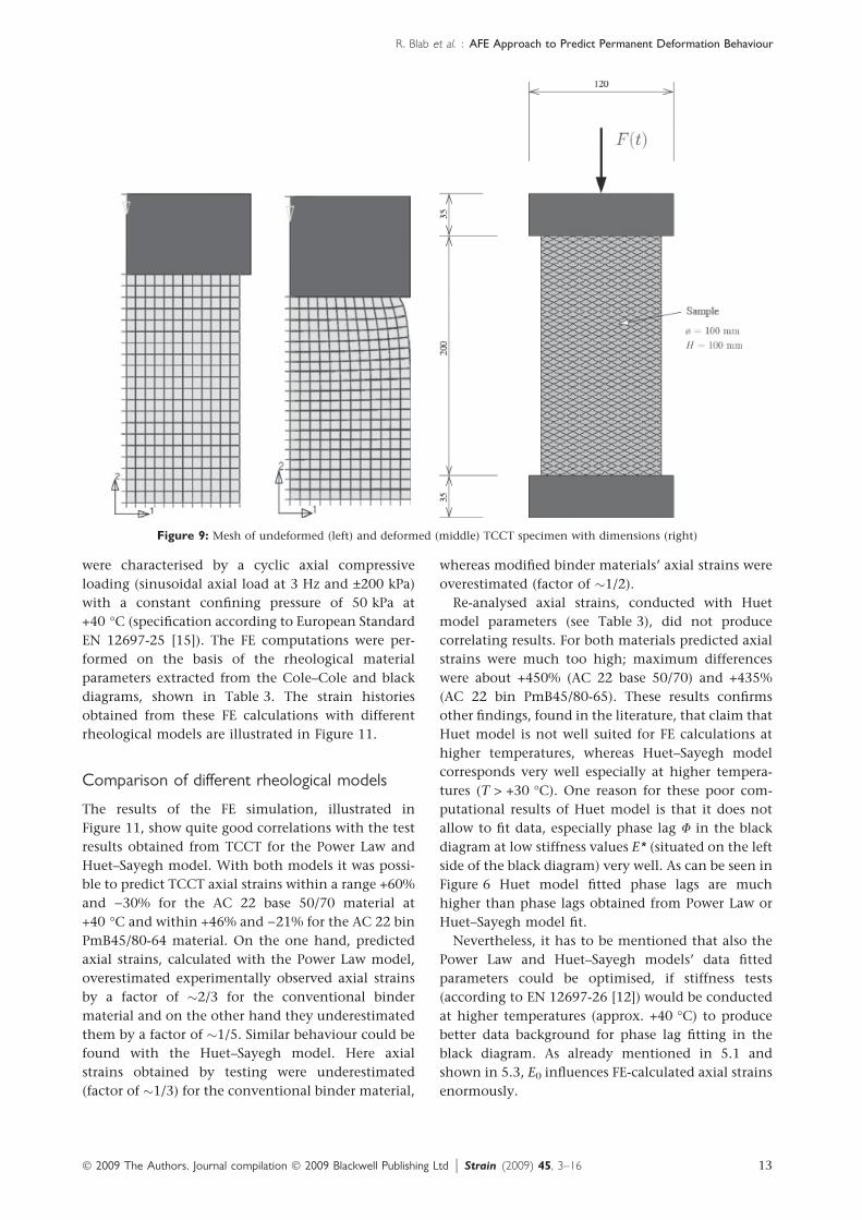
12697-25 [15]. Exploiting the axisymmetry of the

problem, a two-dimensional axisymmetric model

was chosen. Moreover, the symmetry with respect to

the horizontal centreline was taken into account

reducing the FE model to one-quarter of the cylin-

drical specimen (outlined in Figure 9).

The geometric dimensions of the triaxial test set-up

are shown in Figure 10. In addition to the asphalt

specimen, the loading platen was considered in the

FE analysis. The cyclic, dynamic axial force was

applied onto this loading platen.

As observed during the experimental laboratory

work, the asphalt specimen experienced non-uni-

form deformations, characterised by increasing radial

deformation with increasing distance from the load-

ing platen. This effect, more pronounced in case of

higher testing temperature and large testing time, is

explained by the lateral confinement at the loading

platen. Accordingly, a contact formulation consider-

ing friction between the asphalt specimen and the

loading platen was considered in the numerical

analyses (friction according to Coulomb’s law with

l¼ 0.8). According to the numerical results presented

in this paper, uniform strain and stress distributions

were obtained in the main part of the specimen for

height/diameter ratios equal to and higher than 200/

100 (shown in Figure 10; axial displacements

homogenous; radial displacements influenced by

friction effects between loading platen and speci-

men). Laboratory tests of the two materials (AC 22

base 50/70 and AC 22 bin PmB 45/80-65) described in

chapter 2 were re-analysed. The chosen experiments

2.8 %

–4.0 %

0.0 %

–0.3 %0.0 %

0.2 %

–10–8–6–4–202468

10

original+1% original–1%

E Ja k

5.3 %

75.8 %

9.5 %0.0 %

–3.2 %

–50.5 %

–7.4 %–18.9 % –26.3 %

87.4 %

6.3 %

0.0 %

–100–80–60–40–20

0

20406080

100

original+1% original–1%

E0 E Ja k Jb h

Figure 7: Graphical illustration of relative error’s proportional change for variation of Power Law parameters (left side) and Huet–

Sayegh parameters (right side) ±1% of the optimum of material AC22 base 50/70

2.3 %

–3.0 %

0.0 %

–0.4 %

0.4 %

0.0 %

–10–8–6–4–202468

10

Original+1% Original–1%

E Ja k

4.4 %10.7 %

5.0 %9.9 %

–0.3 %

–13.5 % –11.0 %

–27.3 %

–4.1 %

12.7 %6.3 %

–5.0 %

–50–40–30–20–10

01020304050

Original+1% Original–1%

E0 E J ka Jb h

Figure 8: Graphical illustration of relative error’s proportional change for variation of Power Law parameters (left side) and Huet–

Sayegh parameters (right side) ±1% of the optimum of AC22 bin PmB 45/80-65



were characterised by a cyclic axial compressive

loading (sinusoidal axial load at 3 Hz and ±200 kPa)

with a constant confining pressure of 50 kPa at

+40 �C (specification according to European Standard

EN 12697-25 [15]). The FE computations were per-

formed on the basis of the rheological material

parameters extracted from the Cole–Cole and black

diagrams, shown in Table 3. The strain histories

obtained from these FE calculations with different

rheological models are illustrated in Figure 11.

Comparison of different rheological models

The results of the FE simulation, illustrated in

Figure 11, show quite good correlations with the test

results obtained from TCCT for the Power Law and

Huet–Sayegh model. With both models it was possi-

ble to predict TCCT axial strains within a range +60%

and )30% for the AC 22 base 50/70 material at

+40 �C and within +46% and )21% for the AC 22 bin

PmB45/80-64 material. On the one hand, predicted

axial strains, calculated with the Power Law model,

overestimated experimentally observed axial strains

by a factor of �2/3 for the conventional binder

material and on the other hand they underestimated

them by a factor of �1/5. Similar behaviour could be

found with the Huet–Sayegh model. Here axial

strains obtained by testing were underestimated

(factor of �1/3) for the conventional binder material,

whereas modified binder materials’ axial strains were

overestimated (factor of �1/2).

Re-analysed axial strains, conducted with Huet

model parameters (see Table 3), did not produce

correlating results. For both materials predicted axial

strains were much too high; maximum differences

were about +450% (AC 22 base 50/70) and +435%

(AC 22 bin PmB45/80-65). These results confirms

other findings, found in the literature, that claim that

Huet model is not well suited for FE calculations at

higher temperatures, whereas Huet–Sayegh model

corresponds very well especially at higher tempera-

tures (T > +30 �C). One reason for these poor com-

putational results of Huet model is that it does not

allow to fit data, especially phase lag U in the black

diagram at low stiffness values E* (situated on the left

side of the black diagram) very well. As can be seen in

Figure 6 Huet model fitted phase lags are much

higher than phase lags obtained from Power Law or

Huet–Sayegh model fit.

Nevertheless, it has to be mentioned that also the

Power Law and Huet–Sayegh models’ data fitted

parameters could be optimised, if stiffness tests

(according to EN 12697-26 [12]) would be conducted

at higher temperatures (approx. +40 �C) to produce

better data background for phase lag fitting in the

black diagram. As already mentioned in 5.1 and

shown in 5.3, E0 influences FE-calculated axial strains

enormously.

Figure 9: Mesh of undeformed (left) and deformed (middle) TCCT specimen with dimensions (right)



TCCT FE simulation with constitutive driver

To validate the sensitivity of the presented rheologi-

cal models to a change in the model parameters,

triaxial cyclic compression tests (TCCT) on cylindri-

cal specimens were re-analysed. Because of the

uniform stress state in the sample, the constitutive

driver, only calculating one stress point in the spec-

imen, was used to reduce calculation time.

Again, two materials (AC 22 base 50/70 and AC 22

bin PmB 45/80-65) described in chapter 2 were used

for this sensitivity analysis, carried out on two rheo-

logical models (Power Law model and Huet model).

The material parameters extracted from the Cole-

Cole and black diagrams, shown in Table 3 were used

as origin parameters for this analysis. The variation of

material parameters was chosen by +1% each. Later,

the calculated axial strains after 10 000 load cycles

obtained from the original parameters were com-

pared with the strain history obtained from each

parameter variation. Hereby, the following error

definition (the change in FE-calculated axial strains

De divided by the change in the rheological model

parameter Dparameter) was used.

f ¼ De=Dparameter (38)

These errors are illustrated in Figure 12 for the

Power Law model and in Figure 13 for the Huet

model at three different temperature levels.

The results for the Power Law model showed a

decrease in error for E¥, Ja and k values (be aware of

different units in error definition) from high to low

temperature levels resulting from the decrease in

absolute strain. The failure obtained from a change in

E¥ did not change its value and defined E¥ as a sure

parameter (a variation did not change the result very

much). The weight of the failure obtained from a

change in Ja in comparison with a change in k arised

with dropping temperature (the influence of Ja in

comparison with k arises).

The results obtained from the calculations for the

Huet model again show a decrease in failure from

high to low temperatures and a parameter E¥ that did

not influence the result in a critical manner. At

higher temperatures, only the influence of the short-

term creep parameters (Jb and h) could be seen. When

dropping the temperature, the long-term damper (Jaand k) was activated. The parameters Jb and h lost

weight in comparison with the parameters Ja and k

when leaving the high-temperature regime.

Conclusions

In this paper, constitutive representations of advanced

linear and nonlinear rheological material models (i.e.

Power Law, Huet and Huet–Sayegh model) and their

implementation in a FE code have been presented.

Furthermore, methods are given to derive model

parameter for two specific HMA by means of data fit-

ting with laboratory test data obtained from stiffness

tests according to European Standard EN 12697-26

[12]. Although the considered rheological models

seem to fit very well for the Cole–Cole representations

(diagram consisting of elastic part E1 and viscous part

E2 of the dynamic stiffness values), they did not fit that

properly in the black diagrams representations (dia-

gram consisting of dynamic modulus E* and phase

angle U). For appropriate prediction of permanent

deformations of HMA, occurring at higher tempera-

tures (T > +30 �C), by means of the these rheological

models it is therefore especially important to obtain

Figure 10: Graphical distribution of radial (left) and vertical

(axial) displacements in mm (right) of the deformed TCCT

specimen after 25 000 load cycles (calculated with Huet–Sayegh

model)



stiffness and phase lag values also at elevated temper-

atures. Based on a thorough conducted sensitivity

analysis those model parameters have been identified

which should be select especially careful, i.e. in the

Huet–Sayegh model E0 has enormous influences on

the results of re-analysed axial strains. These were

proven by FE calculations simulating triaxial cyclic

compression tests on cylindrical HMA specimen. E0

can only be fitted properly if adequate test data (phase

angle and dynamic modulus) at elevated temperatures

are available.

The research further shows, that the values of the

obtain model parameters can directly be linked to

material characteristics, e.g. the type of binder that

was used for the asphalt mixes, when modified

binder PmB45(70-65) showed higher glass modulus

0 1 2 3 4 5 6 7 8 9

10

0 2000 4000 6000 8000 10 000

Time (s)

Axi

al s

trai

ns (

%)

AC22 base 50/70 (MV tests) FEAP_Power-Law FEAP_Huet FEAP_Huet-Sayegh

0.1

1

10

1 10 100 1000 10 000Time (s)

Axi

al s

trai

ns (

%)

0 1 2 3 4 5 6 7 8 9

10

0 2000 4000 6000 8000 10 000

Time (s)

Axi

al s

trai

ns (

%)

AC22 bin PmB45/80-65 (MV tests) FEAP_Power-Law FEAP_Huet FEAP_Huet-Sayegh

0. 1

1

10

1 10 100 1000 10 000Time (s)

Axi

al s

trai

ns (

%)

AC22 bin PmB45/80-65FEAP_Power-LawFEAP_HuetFEAP_Huet-Sayegh

AC22 base 50/70 FEAP_Power-Law FEAP_Huet FEAP_Huet-Sayegh

Figure 11: Time-axial strain history of TCCT test results (+40 �C) and FE simulation (rheological model parameters for +40 �C)

in linear scale (left side) and logarithmic scale (right side) for AC 22 base 50/70 (upper lane) and the AC 22 bin PmB 45/80-65

materials (lower lane)

+40 °C

0.00E+00

2.00E-04

4.00E-04

6.00E-04

8.00E-04

1.00E-03

1.20E-03

1.40E-03

1.60E-03AC22 base 50/70AC22 bin PmB 45/80-65

+1% E +1% Ja +1% k

+15 °C

0.00E+00

5.00E-06

1.00E-05

1.50E-05

2.00E-05

2.50E-05

3.00E-05

3.50E-05

4.00E-05

4.50E-05


+1% E +1% Ja +1% k

–10 °C

–5.00E-06

–4.00E-06

–3.00E-06

–2.00E-06

–1.00E-06

0.00E+00

1.00E-06

2.00E-06

3.00E-06

AC22 base 50/70AC22 bin PmB 45/80-65

+1% E +1% Ja +1% k

Figure 12: Failure values obtained from calculations with the Power Law model in the constitutive driver after 10 000 load cycles.

Variation of each material parameter of 1% for AC 22 base 50/70 and the AC 22 bin PmB 45/80-65 materials. Calculated temper-

atures: 40, 15 and )10 �C



values E¥ than conventional binders (50/70). In a

next step a database with model parameters of

different HMA types and binders will be established

to more accurately investigate the influences of

binder type and HMA composition. These correla-

tions can then be used for the prediction of per-

manent deformation behaviour of different HMA

types within FE simulations of flexible pavement

constructions.

REFERENCES

1. Huet, C. (1963) Etude par une methode d’impedance du

comportement viscoelastique des materiaux hydrocarbones.

PhD thesis. Faculte des Sciences de l’Universite de Paris,

Paris (in French).

2. Sayegh, G. (1965) Variation des modules de quelques bitumes

purs et enrobes bitumineux. These de doctorat d’ingenieur,

Faculte des Sciences de l’universite de Paris (in French).

3. Lai, J. S. and Hufferd, W. L. (1976) Predicting permanent

deformation of asphalt concrete from creep tests. Trans-

portation Research Record 616, Transportation Research

Board, Washington, DC.

4. Sides, A., Uzan, J. and Perl, M. (1985) A comprehensive

visco-elastoplastic characterization of sand-asphalt under

compression and tension cycle loading. J. Test. Eval., 13/1,

49–59.

5. Schapery, R. A. (1999) Nonlinear viscoelastic and visco-

plastic constitutive equations with growing damage. Int. J.

Fract., 97, 33–66.

6. National Cooperative Highway Research Program NCHRP

(1999) Advanced AC mixture material characterization mod-

els framework and laboratory test plan. Final Rep., Submitted

to: NCHRP 9-19, Superpave Support and Performance

Models, Arizona State University, Superpave Models

Team, Washington, DC.

7. Uzan, J. and Levenberg, E. (2007) Advanced testing and

characterization of asphalt concrete materials in tension.

Int. J. Geomech., 03/04, 158–165.

8. Di Benedetto, H., Olard, F., Sauzeat, C. and Delaporte, B.

(2004) Linear viscoelastic behaviour of bituminous mate-

rials: from binders to mixes. Int. J. Road Mater. Pavement

Des., 5, Special Issue EATA, 163–202.

9. Di Benedetto, H., Delaporte, B. and Sauzeat, C. (2007)

Three-dimensional linear behavior of bituminous materi-

als: experiments and modeling. Int. J. Geomech., 03/04,

149–157.

10. Desai, C. S., Somasundaram, S. and Frantziskonis, G.

(1986) Hierarchical approach for constitutive modeling of

geologic materials. Int. J. Numer. Anal. Methods Geomech.,

10, 225–257.

11. Molenaar, A. A. A. (2006) Asphalt mechanics, a key tool for

improved pavement performance prediction. Proceedings, II

European Conference on Computational Mechanics, Lis-

bon, Portugal, 5–8 June 2006.

12. EN 12697-26 (2005) Asphalt – Test Methods for Hot Mix

Asphalt – Part 26: Stiffness. Comite europeen de normali-

sation CEN, Brussels, 2004-10-01.

13. Findley, W. N., Lai, J. S. and Onaran, K. (1989) Creep and

Relaxation of Nonlinear Viscoelastic Materials. Dover Publi-

cations Inc., New York.

14. Blab, R., Kappl, K., Lackner, R. and Aigner, E. (2006) Per-

manent Deformation of Bituminous Bound Materials in Flex-

ible Pavements – Evaluation of Test Methods and Prediction

Models. SAMARIS D28 Main Report, Vienna.

15. EN 12697-25 (2004) Asphalt – Test methods for hot mix

asphalt – Part 25: Cyclic compression test. Comite europeen

de normalisation CEN, Brussels, 2004-12-01.

+40 °C

0.00E+00

5.00E-03

1.00E-02

1.50E-02

2.00E-02

2.50E-02

3.00E-02

3.50E-02

4.00E-02


+1% E +1% Ja +1% k +1% Jb +1% h

+15 °C

0.00E+00

1.00E-05

2.00E-05

3.00E-05

4.00E-05

5.00E-05

6.00E-05

7.00E-05

8.00E-05

9.00E-05


+1% E +1% Ja +1% k +1% Jb +1% h

–10 °C

–2.50E-06

–2.00E-06

–1.50E-06

–1.00E-06

–5.00E-07

0.00E+00

5.00E-07

1.00E-06

AC22 base 50/70AC22 bin PmB 45/80-65

+1% E +1% Ja +1% k +1% Jb +1% h

Figure 13: Failure values obtained from calculations with the Huet model in the constitutive driver after 10 000 load cycles.

Variation of each material parameter of 1% for AC 22 base 50/70 and the AC 22 bin PmB 45/80-65 materials. Calculated temper-

atures: 40, 15 and )10 �C



a finite-element approach to predict permanent deformation

Documents