N A S A C O N T R A C T O R

R E P O R T

N A S A C R - 2 4 0 6

A CURVATURE-CORRECTED KIRCHOFF

FORMULATION FOR RADAR SEA-RETURN

FROM THE NEAR VERTICAL

by Frederick C. Jackson

Prepared by

NEW YORK UNIVERSITY

for Langley Research Center

NATIONAL AERONAUTICS AND SPACE ADMINISTRATION • WASHINGTON, D. C. • APRIL 1974

https://ntrs.nasa.gov/search.jsp?R=19740012866 2018-07-29T08:54:44+00:00Z

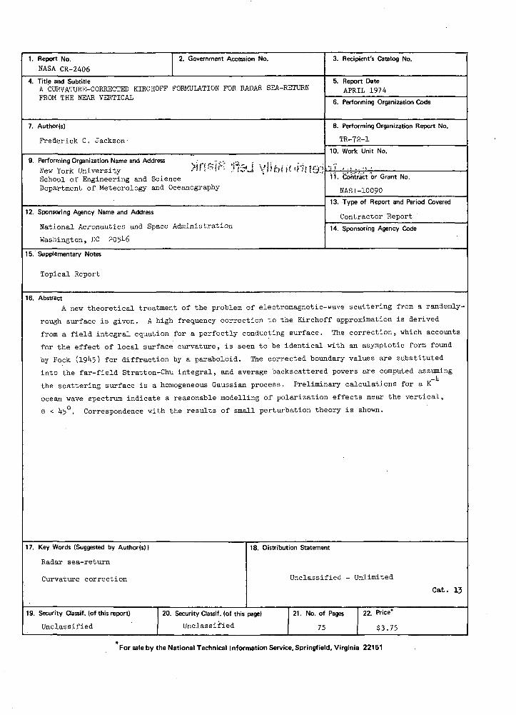
1. Report No.NASA CR-2406

4. Title and Subtitle

2. Government Accession No.

A CURVATURE-CORRECTED KIRCHOFF FORMULATION FOR RADAK Si^-KKL'UKJS

7. Author(s)

Frederick C . Jackson

9. Performing Organization Name and Addressw v v rr • n-

',- .-,>if {£{»"•• ~>l=?-i v 'MKji ' i r fn^nSchool of Engineering and ScienceDepartment of Meteorology and

12. Sponsoring Agency Name and Address

Oceanography

;

National Aeronautics and Space Administration

Washington, DC 205^6

15. Supplementary Notes

Topical Report

16. AbstractA new theoretical treatment of the problem

3. Recipient's Catalog No.

5. Report DateAPRIL 1974

6. Performing Organization Code

8. Performing Organization Report No.

TR-72-110. Work Unit No.

: ': 1 » . ! . . - • » •11. Contract or Grant No.

NAS1-10090

13. Type of Report and Period Covered

Contractor Report

14. Sponsoring Agency Code

of electromagnetic-wave scattering from a randomly-

rough surface is given. A high frequency correction to the Kirchoff approximation is derived

from a field integral equation for a perfectly conducting surface. The correction, which accounts

for the effect of local surface curvature, is seen to be identical with an asymptotic form found

by Fock (19^5) for diffraction by a paraboloid. The corrected boundary values are substituted

into the far-field Stratton-Chu integral, and average backscattered powers are computed assuming

the scattering surface is a homogeneous Gaussian

ocean wave spectrum indicate

8 < 1*5°. Correspondence with

process . Preliminary calculations for a K

a reasonable modelling of polarization effects near the vertical,

the results of small perturbation theory is shown.

17. Key Words (Suggested by Author(s))

Radar sea-return

Curvature correction

19. Security dassif. (of this report) 2

Unclassified

0. Security Classif . (of this

Unclassified

18. Distribution Statement

Unclassified - Unlimited

Cat. 13

page) 21. No. of Pages 22. Price*

75 $3.75

For sale by the National Technical Information Service, Springfield, Virginia 22151

TABLE OF CONTENTS

Summary v

I. Introduction 1

1.1 Origins 1

1.2 Rough-surface scattering theory and radarsea-return 1

1.3 Outline . 5

II. The Randomized Kirchoff Method According toBeckmann 6

III. On the Nature of the Kirchoff Solution. Radar-SeaReturn 15

3.1 The stationary phase approximation 15

3.2 The "small perturbation" approximation 19

3.3 Radar sea-return. The idea of a compositesurface' 21

IV. Results of Small Perturbation Theory 27

V. A High Frequency Correction to the KirchoffApproximation ' 30

VI. Calculation of the Scattered Power 40

VII. Properties of the Solution 51

7.1 Comparison with first-order Rayleigh-Ricetheory i 51

7.2 A sample calculation: Copolarized returnsfrom an isotropic K~ spectral-law surfaceand a one-dimensional K~^ spectral-law surface . 52

VIII. Discussion and Conclusions to be Drawn. . 60

References 65

Appendix 69

ill

LIST OF FIGURES

Fig. No.

1 The scattering situation „ 7

2 Defining geometry and notation 7

3 Two-dimensional Kirchoff solution for a K"^ spectral-law surface 24

4 Stationary phase and small perturbation approximationsto the Kirchoff integral 26

5 The "composite surface" solution as sum ofstationary phase and small perturbation cross-sect ions . . . 26

6 First-order Rayleigh-Rice solution 29

7 Three-dimensional corrected Kirchoff solution for co-polarized returns from an isotropic K~ spectral-lawsurface 56

8 Two-dimensional corrected Kirchoff solution for co-polarized returns from a K"^ spectral-law surface 57

9 Ocean backscatter data showing cross-over of copolarizedreturns 58

Summary

A new theoretical treatment of the problem of electromagnetic

wave scattering from a randomly-rough surface is given. A high fre-

quency correction to the Kirchoff approximation is derived from a

field integral equation for a perfectly conducting surface. The cor-

rection is of the form J_ = S J where J is the Kirchoff value

of the current density, and S is a linear function of the second de-

rivatives of surface height. The correction is seen to be identical'to

an asymptotic form found by Fock (1945) in his investigation of dif-

fraction by a convex paraboloid.

The corrected current density is substituted into the far-

field Stratton-Chu integral, and average backscattered powers for

the four linear polarization combinations are computed on the as-

sumption that the scattering surface is describable as a homogeneous

Gaussian random process.

The strength of the solution is that local diffraction effects

(arising from surface curvature) are properly correlated with surface

height and slope without requiring their smallness.

Application to radar backscatter and natural microwave

emission from the sea is discussed. It is concluded that this "cor-

rected Kirchoff" formulation offers a superior predictive capacity for

co-polarized and depolarized returns from the near vertical, 9 < 45°.

Extension to the bistatic case is recommended for application to the

natural emission problem. The evolution of a new "composite" model

of backscatter combining this solution with small perturbation results

suggests itself.

I. Introduction

1.1 Origins

A satellite-borne combination radar-radiometer has been

proposed as a remote sensing device for monitoring wind field/wave

field conditions over the world ocean (see, for a recent version of

this proposal, Moore and Pierson, 1971). This proposal has st imu-

lated much of the recent theoretical and experimental work on radar

backscatter and natural microwave emission from a wind-roughened

sea. In particular, the research reported here was motivated by a

need for a broader theoretical basis for understanding and predict-

ing microwave scattering by the sea. A go^od part of this research

has been previously documented in a New York University technical

report (Jackson, 1971).

1.2 Rough surface scattering theory and radar sea-return

The general problem of electromagnetic-wave scattering

from a plane rough surface has been approached in a variety of ways.

Some authors have dealt with exact solutions for scattering from

certain simple (idealized) surfaces such as a surface composed of

periodic rectangular corrugations (Deryugin, I960). Exact solutions

for arbitrary surfaces can be obtained by the numerical solution of

an integral equation for the surface field (Lenz, 1971). Except for

one-dimensional surfaces possessing a small amount of structure

(e. g. , a small number of "hills" and "valleys") the computational

time is prohibitive. Many analytical methods have been developed

for the class of surfaces which can be called slightly rough, defined

as having small slopes and heights small compared to the wavelength.

Exact solutions for deterministic slightly rough surfaces can be ob-

tained by Rayleigh's method, or Meecham's (1956) variational tech-

nique. Rayleigh's method has been randomized by Rice (1951) , and

this provides one of the most powerful methods for handling scatter-/

ing from randomly rough surfaces. Twersky (1957) has used a Ray-

leigh image method for computing exactly the scattering by a random

array of "bosses" or protuberances on a plane. Exact methods--

while impractical for application to randomly rough surfaces with

a high degree of "structure"--can be very useful in the testing of

approximate methods developed for general classes of randomly

rough surfaces.

Some authors have taken conceptual approaches which

are at the same time simple and instructive --for example, Katzin 's

(1957) slope-facet model and Long's (1965) dipole model of sea re-

turn. Katzin's model is interesting, for it entertains an important

property of radar sea-return, that near vertical incidence (radar

pointing downward) the backscatter mechanism is dominantly

specular reflection, while backscatter from large angles of incidence

is controlled by diffraction processes. KatzLn's model has been ex-

tended by Rouse (1970).

Of approximate methods which have found practical appli-

cation to scattering from continuously distr ibuted random rough

surfaces, there are essentially three:

a) Geometrical optics

b) Physical optics (Ki rchof f theory)

c) Small perturbation (RayleLgh-R ice theory).

Geometrical optics (or ray optics) formulations, because of

their great simplification of the electromagnetic problem, are cap-

able of handling such phenomena as shadowing and multiple scatter-

ing (Lynch and Wagner, 1970). In considering the generally mild

slopes of ocean surface waves, a ray-optical type of multiple scatter-

ing is not likely to be a significant part of the backscatter mechanism.

In the general bistatic case, however, the process of multiple

reflections may be important. Shadowing effects can similarly be

ignored for angles removed from grazing incidence. Shadowing

is to a f i rs t approximation a simple enough process that it can be

included in a-physical optics formulation (Sancer , 1969).

Most of the work in the last decade has been based upon

either (or both) physical optics (randomized Kirchoff method) or

methods of small perturbation. The randomized Kirchoff method

developed by Beckmann (Beckmann and Spizzichino, 1963, Chs. 3

and 5) and others uses the physical optics (Helmholtz) integral

with the so-called Kirchoff or tangent-plane approximation to the

boundary values of the field. The Kirchoff method is good for softly

undulating surfaces having everywhere a local radius of curvature

large compared to the electromagnetic wavelength. An advantage

of the Kirchoff method (over small perturbation methods) is that

surface height variations do not necessarily have to be small com-

pared to the radar wavelength. A shortcoming of Kirchoff

theory is that with its tangent-plane approximation it cannot account

for polarization effects. Apart from its inability to account for

polarization effects, Kirchoff theory has suffered because its in-

herent strength was not exploited. Often, "what amounts to a station-

ary phase approximation to the Kirchoff integral is made. The

stationary phase approximation is equivalent to geometrical optics;

so, the ability to account for diffraction effects is lost. Chia (1968),

in applying Kirchoff theory to radar sea-return, appears to be the

first to have avoided this approximation by using a realistic wave-

height covariance function in the Kirchoff integral.

Small perturbation theory has gained increasing favor in

the last few years among scientists working on radar sea-return.

This is primarily because of its ability to account for polarization

effects but also because of its simplicity. The explicit dependence

on the wave-height spectrum pointed the way to using a realistic

representation of the rough sea surface (Valenzuela, 1968; Wright,

1968). Small perturbation methods have been developed by several

authors (Bass, 1961; Wright, 1966), notably by R ice (1951). Rice's

randomized Rayleigh method seems to be the superior, for it is capable

of iteration to higher order in height and slope, and is capable of pre-

dicting depolarization in the plane of incidence (Valenzuela, 1967,

1968). The Rayleigh-Rice method--although having some com-

monality with the Kirchoff method--is a fundamentally different

approach to the scattering problem; whereas Kirchoff theory is a

high frequency treatment, Rice's theory is a low frequency method.

In the high frequency approximation, the field in the vicinity of a

surface point is dependent only on the local geometry of the surface,

i. e. , height and slope. In the Rayleigh approach, the field at a point

is related to integral properties (rather than local properties) of the

surface. This local versus integral (or modal) duality in electro-

magnetic theory is discussed by Felsen (1964) in his review of high

frequency diffraction.

1.3 Outline

The theoretical approach taken in this work is a high-

frequency one, and is essentially an extension of the randomized

Ktrchoff method. A curvature correction to the Kirchoff approxi-

mation is derived from a field integral equation, and the corrected

boundary values are used in the Stratton-Chu far-field integral

(vector form of the Helmholtz integral).

In the following section, Beckmann's development of scalar

Kirchoff theory is recapitulated in order to place the theory of

Sections V and VI in its proper perspective. Section III contains

a discussion of the Kirchoff solution, and presents the results

of Kirchoff theory applied to a scattering surface with a K spectral

law. Section IV presents the results of small perturbation theory.

Because of the complexity of the scattering integrals arrived at

and their requirement of a detailed knowledge of the wave-height

covariance function, no thorough computation and comparison with

sea-return data is made. However, some sample calculations are

given, the nature of the solution is discussed and estimates of its

strength are made.

II. The Randomized Kirchoff Method According to Beckmann'''

Consider bhe scattering situation depicted in Fig . 1.

A monochromatic source (radar) illuminates a portion S of a rough

conducting surface. Beckmann. deals with the scalar electric field

E scattered by the surface. The surface field vanishes outside of

S , and the scattered field satisfies the radiation condition at

infinity. The electric field scattered toward an observation point

P is given by the Helmholtz integral involving the (unknown) field

boundary values:

QE\^ 12 M-5-- dS (i. 1)

s°where E is the total electric field or. the surface; 3/8n stands

for the normal derivative directed outwards (upwards) from the

conducting volume; and G is the Green 's function for (three-

dimensional) free space,

-ikr

° = f-where k is the microwave propagation constant and r is the

distance from source points on the surface to the observation

point. If P is in the far-f ie ld (Fraunhofer zone) r can be

Beckmann and Spizzichino (1963), Chapters 3 and 5.

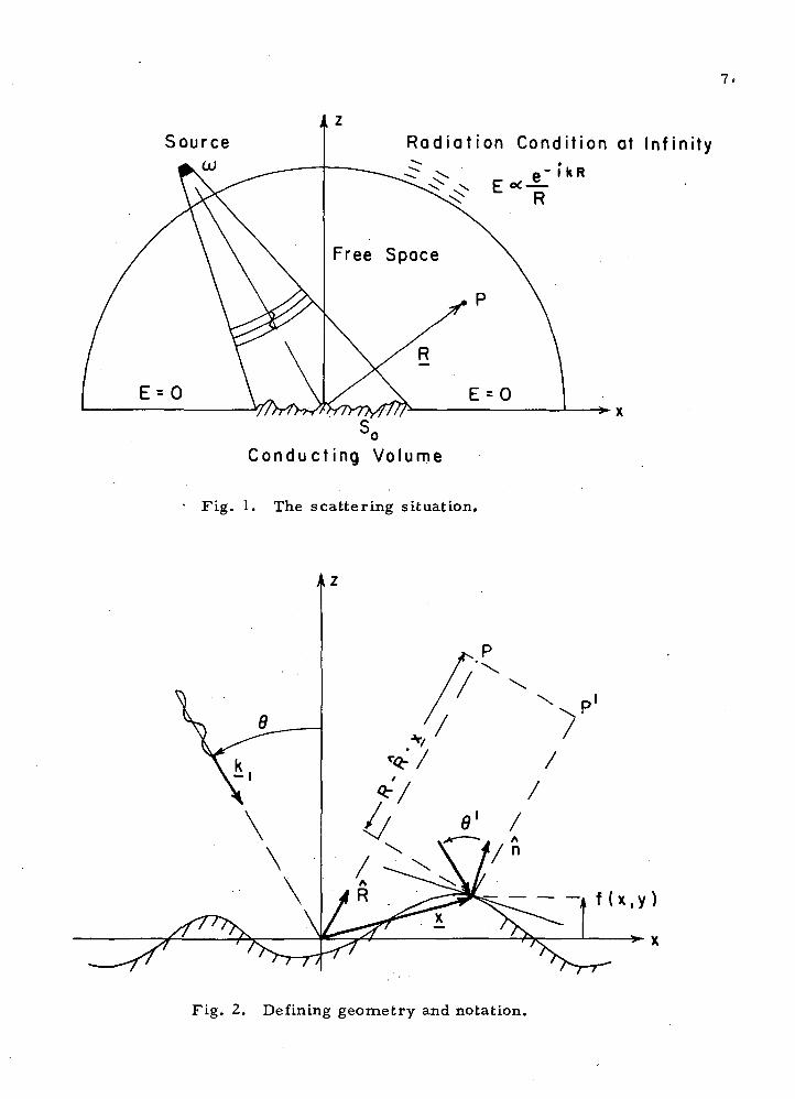
R a d i a t i o n Condi t ion at Inf ini ty

- | k R

C o n d u c t i n g Volume

Fig. 1. The scattering situation.

Fig. 2. Defining geometry and notation.

approximated byv

r ~R - R -x (2.3)

where R_ = R R is the position vector of P and x is the coordinate

vector of surface source points. With this approximation, we can write

G =

and

- ikR ikR • x£ • e —R

n G

(2.4a)

(2.4b)

!;:Here, Beckmann fails to give any criterion for deciding how farremoved the observation point must be to lie within the Fraunhoferdiffract ion zone. A criterion can be established, however, withouttoo much difficulty. The phase error incurred in making the far-field approximation is (see accompanying figure):

2lT(XP - QP )

2ir 1 2~ — ' 2 a '

With a ~x cos 9/R, and

setting QP ~ OP = R

., TTX COS 9Am «^* ————^—^ XR

The first Fresnel zone is at = IT, so that x~ \/XR sec 9.

x

For example, with a 10 cm radar at an (aircraft) altitude of1 km, x^ 10 m - 100\; or, at a (spacecraft) altitude of 1000 km,

100 m = 1000X. For deep fade conditions (rms surface heightmuch larger than radar wavelength), the surface source field be-comes incoherent well within one -hundred radar wavelengths.Only under laboratory conditions and/or the condition of smallroughness amplitude need Fresnel zone effects be considered(see, for example, Wright and Keller, 1971).

I

where n is the unit outward surface normal.

The incident field E is taken to be a plane wave''" of unit

amplitude. With the time-harmonic dependence e w suppressed, El

is written as the phasor,

(2.5)

where Js^ is the propagation vector of the incident wave.

The Kirchoff approximation to the field boundary values E

and 3E/3n consists in assuming that the field in the vicinity of (an

"epsilon" neighborhood) and at a point on the surface is nearly equal

to the field which would exist on an infinite tangent plane at the point.

This is a type of "high frequency" approximation. For a high enough

microwave frequency (wave number), the surface curvature "appears"

mild to the radiation and the surface can be considered to be locally

flat. There is then a perfect reflection of the incident wave in

accordance with the geometrical optics Law of Reflection; the ampli-

tude and phase of the reflected wave are given by Fresnel's formulas.

Then, writing the field in the vicinity of the surface as an incident

wave plus a reflected wave, we have for the total field and its normal

derivative evaluated on the surface:

E = (1 + fiOE (2.6a)

- i k - n f l - R ) E L . * * (2.6b)

* The justif ication for ignoring the sphericity of an incident waveradiated by a point source (radar) follows the same argumentsgiven for the far-zone approximation on the scattered field (seeprevious footnote).

**In writing (2.6) with the incident wave EL given by eq. (2.5), it istacitly assumed that there is no multiple scattering nor shadowing.

10

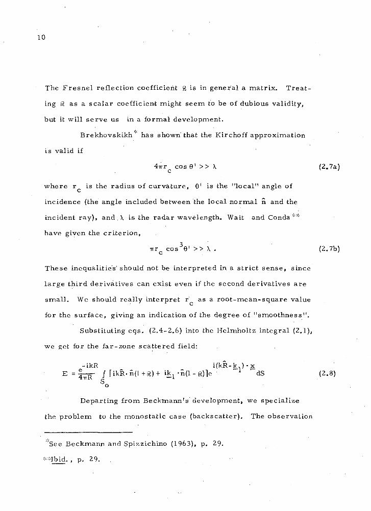
The Fresnel reflection coefficient (ft, is in general a matrix. Treat-

ing fa as a scalar coefficient might seem to be of dubious validity,

but it will serve us in a formal development.O'

Brekhovskikh"" has shown" that the Kirchoff approximation

is valid if

4-rrr cos 9' » \ (2.7a)

where r is the radius of curvature, 9' is the "local" angle ofC

incidence (the angle included between the local normal n and the

incident ray), and X is the radar wavelength. Wait and Conda**

have given the criterion,

irr cos39' » X . (2.7b)

These inequalities* should not be interpreted in a strict sense, since

large third derivatives can exist even if the second derivatives are

small. We should really interpret r as a root-mean-square valueC

for the surface, giving an indication of the degree of "smoothness".

Substituting eqs. (2.4-2.6) into the Helmholtz integral (2.1),

we get for the far-zone scattered field:

e-ikR ^ ^ i(kR-k )-xE = 47R- n ^ - n d + ^ + ^ - n d - ^ e

Departing from Beckmann's development, we specialize

the problem to the monostatic case (backscatter). The observation

""See Beckmann and Spizzichino (1963), p. 29.

--Ibid. , p. 29.

11

point then coincides with the source, and the incident propagation

vector can be written as k, = -kR . Eq. (2.8) becomes:

E = Eft / 2 f t R - n e L 2 k R ' £ dS (2.9)"

We adopt the following notation (Fig. 2): Let the surface be

described in the (x, y, z) Cartesian system by

z = f(x, y) .

The coordinate vector of surface points is then

x = (x, y, f)

The normal vector is given by

n = (-fx, -f , l )cosw ,

where f and f are partial derivatives. The surface area elementx 7

is given by

dS = sec w dx dy .

The plane of incidence is formed by R and the z-axis. The x and y

axes are oriented so" that the x-axis lies in the plane of incidence. The

angle of incidence 9 is measured positive where the incident ray comes

from the left (negative x-direction). The unit vector R is given by

R = (-a, 0 , < y )

where

a = ' s in 9

•y = COS 9 •

Equation (2.9) becomes

12

ikRE = / / 2 « ' ( V + a f ) - e - - V d y (2.10)

where A is the (horizontal) illuminated area. Now assume for

the moment that the surface is perfectly conducting. Then, R = ±1

(the sign depending on polarization) and ft can be treated as a con-

stant and removed from under the integral.''' With R = ±1, (2.10)

is integrated by parts to yield

E = ± £ % l R«- f7 e- I 2 k ( a X-Vf)dx'dy+ "edge terms" . (2.11)'

For large areas k A » 1, the edge terms are negligible. This

is not obvious from the form of (2.11); but, it is physically reasonable

that — provided the surface is moderately rough and grazing incidence

is avoided- -edge effects are unimportant in the scattering problem.

The average backs cattered power is proportional to < |E| ) where the

brackets denote expectation, or ensemble average. Neglecting the

edge terms, we form |E| = EE* as a two-fold integral over A , and take

the average over all realizations of the surface:

2f f f f . i2kv(f1-f)\ -i2ka(x'-x) , . , , , , ,-. , 0,

) / / / /< e >e 'dx'dy'dxdy (2.12)

The expectation

} (2.13)

is the two-dimensional characteristic function of the random vector

(f, f) evaluated at (2k-y, - 2k-y). If f is a stationary (homogeneous)

*This is not immediately evident. It turns out, however, that thevector formulation of the Kirchoff integral for perfect conductivityyields precisely (2.10) with the effect of polarization properly accountedfor by the ± sign in front of the integral. (Cf. eqs. 6.2a, d)

13

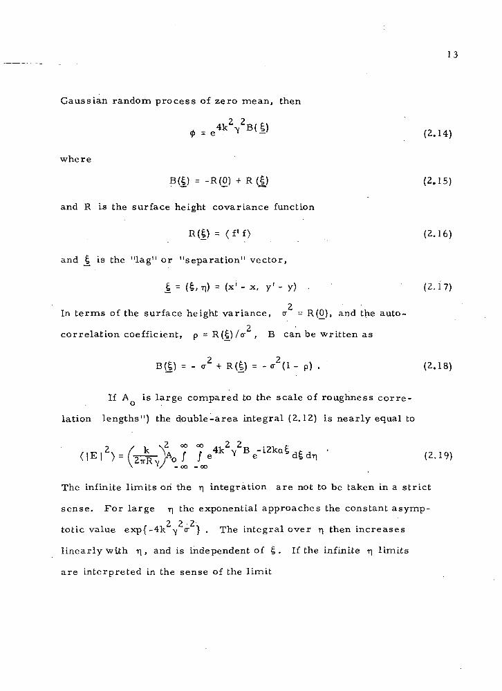
Gaussian random process of zero mean, then

where

B(|) = -R(0) + R(|) (2.15)

and R is the surface height covariance function

R(|) = < £ ' £ > (2.16)

and _£ is the "lag" or "separation" vector,

1= (I.T,) = (x1- x, y'- y) . ' (2.17)

2In terms of the surface height variance, <r = R(0) , and the auto-

correlation coefficient, p = R(£)/O- , B can be written as

B(|) = - <r2 + R(|) = - cr2(l - p) . (2.18)

If A is large compared to the scale of roughness corre-

lation lengths") the double-area integral (2.12) is nearly equal to

OO GO -- Z L* ~, . -*•. f-

! /e^^e-^^dldr, ' (2.19)- oo - oo

The infinite limits on the T| integration are not to be taken in a strict

sense. For large r| the exponential approaches the constant asymp-

2 2 2totic value exp{-4k -y <r } . The integral over r\ then increases

linearly with r\ , and is independent of £ . If the infinite r\ limits

are interpreted in the sense of the limit

14

. . "7 4kv2B - i

lim / / e •" eY — oo - oo - Y

then it is seen that (except for vertical.incidence, a = 0) the

phasor nullifies the constant contribution from large r\ and the integral

exists. In practice we generally deal with very rough surfaces for

2 2. 2which 4k Y °~ » 1 and the exponential for large lag is extremely

small. A numerical integration over n would then be stopped, at some

prescribed value of r| for which the exponential is very small.

Since the covariance function R'($.) is symmetric about

the origin, (2.19) simplifies to

The backscattered power is conventionally given in terms of the

normalized isotropic radar cross section, <r° , defined by

< | E | > . (2.21)

Then, (2.20) becomes

_, 2 . oo oo .2 2o" = • = £ _ . J^./ /e 4 K ^ B cos2kQe d£ dn . (2.22)

•y O - oo

15

III. On the Nature of the Kirchoff Solution. Radar Sea-Return

The KLrchoff integral (2.22) contains information on the two

backscatter regimes: the "specular" (ray-optic) regime which pre-

ponderates for small angles of incidence, and the "small perturbation"

(diffraction) regime which accounts for the backscatter from large

angles of incidence.

3.1 The stationary phase approximation

The high frequency limit of physical optics yields geometrical

optics: symbolically,

lim (physical optics) = geometrical opticsk—»oo

The high frequency limit is equivalent to a case where (1) the surface is

very smooth, and (2) the phase modulation is very deep. The "deep fade"

condition ( Hagfors, 19&4) means we must have (for backscatter):

4k2v

2o-2 » 1 . (3.1)

In the high frequency case characterized by (3.1), the exponential

exp{4k -y B} becomes negligible outside of a small region about the

origin. The meaning of the smoothness condition is that within this

"neighborhood" of the origin, the covariance function can be repre-

sented by a Taylor series truncated at second degree. Thus, we can

write B(|) as the paraboloid:

B = Rxx(0) I' + Rxy(0) *„ + Ryy(0) 2L

Considering (for simplicity) the special case where £ and r\ are the

16

principal axes of the ellipse B - constant, B can be written as

B l 2f2 1 2 2 /, ?\B = - -* <r 5 - - T - O " TI (3.2)2 x 2 y ' '

where tr = -R (0) and a = -R (0) are the slope variances inx xxv— y yythe x and y directions. The rms slope <r is invariant with re-

s

spect to coordinate rotation,

= la- Z + (r 2 (3.3)• V x y x '(T

s V x y

Putting (3.2) into (2.22) and integrating, we find (letting (r °

represent the high frequency limit):

Uan29

2cr cr vX yY

(3.4)

The cross-section (3.4) is independent of k, consistent with the fact

that it is the high frequency limit — geometrical optics. Another way

of seeing that (3.4) is a geometrical optics limit is to note the cr°

is simply proportional to the probability of a surface facet satisfy-

ing the specular (ray-optic) condition for backscatter: f = tan0.JC

For an isotropic surface, cr = cr , and (3.4) becomes

tan 6

(3.5)

For reference, we should like to know the cross-section for a two-

dimensional scattering situation. One has to go back to the Helm-

holtz integral for two dimensions:

17

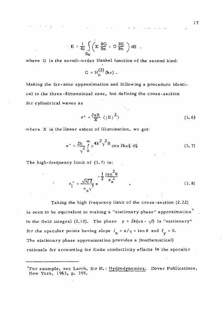
1 (V 8G 9E \E - 41 J (E 3rl - G 8n" ) dS "

So

where G is the zeroth-order Hankel function of the second kind:

G = HQ2) (kr) .

Making the far-zone approximation and following a procedure identi

cal to the three-dimensional case, but defining the cross-section

for cylindrical waves as

< | E | > (3.6)

where X is the linear extent of illumination, we get:

(3.7)

The high-frequency limit of (3.7) is:

1 tan29

N/TT/2 ?"x /7 Q\- e . (3. 8)" VX Y

Taking the high frequency limit of the cross-section (2.22)

is seen to be equivalent to making a "stationary phase" approximation '

to the field integral (2.10). The phase <|> = 2k(ax- ^f) is "stationary"

for the specular points having slope f = a/-y = tan 9 and f =0.

The stationary phase approximation provides a (mathematical)

rationale for accounting for finite conductivity effects in the specular

*For example, see Lamb, Sir H. : Hydrodynamics. Dover Publications,New York, 1963, p. 395.

18

(near vertical) regime. Referring again to eq. (2.10), we see that

R is brought out of the integral and evaluated at the local angle ofi

incidence 9 = 0 for stationary or specular points. This is just

the mathematical version of what we should expect on physical

grounds: that where specular reflection is the dominant mode of

scattering, the backscattered field is composed primarily of incident

waves reflected at locally vertical incidence. Thus, the effect of finite

conductivity it to a f irst approximation (a very good first approximation

for radar return from the sea) simply to reduce the backscattered

signal by a factor of | f t (0 ) | . And this is true regardless of polari-

zation, since at (locally) vertical incidence the distinction between

horizontal and vertical polarization'1" disappears.

Stogryn (1967a) came to this conclusion using a vector

Kirchoff formulation and making the "stationary phase" approximation.

Kaufman (1 971)--apparently unaware of Stogryn's conclusions — used

a vector Kirchoff formulation for finite conductivity, and computed

cross sections for different polarizations. Unfortunately, Kaufman

made the stationary phase approximation, so that no information was

gained on the effects of finite conductivity (as they manifest in a

Kirchoff formulation) in the diffraction regime at larger incidence

angles. For reference, let us write down our conclusion symbolically

as

;;=These terms have not yet been defined. Vertical polarization (V)means the E-vector is in the plane of incidence (mean plane orlocal plane); horizontal polarization (H) means the E-vector is per-pendicular to the plane of incidence, that is, lies in the plane ofthe surface (mean or local).

19

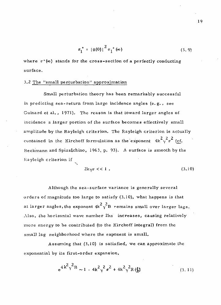
°y(«>) (3.9)

where (r°(oo) stands for the cross-section of a perfectly conducting

surface.

3.2 The "small perturbation" approximation

Small perturbation theory has been remarkably successful

in predicting sea-return from large incidence angles (e.g. , see

Guinard et al. , 1971). The reason is that toward larger angles of

incidence a larger portion of the surface becomes effectively small

amplitude by the Rayleigh criterion. The Rayleigh criterion is actually

contained in the Kirchoff formulation as the exponent 4k y °~ (cf.

Beckmann and Spizzichino, 1963, p. 93). A surface is smooth by the

Rayleigh criterion if

2kyo- « 1 . (3.10)

Although the sea-surface variance is generally several

orders of magnitude too large to satisfy (3.10), what happens is that

at larger angles, the exponent 4k y B remains small over larger lags.

Also, the horizontal wave number 2ka increases, causing relatively

more energy to be contributed (to the Kirchoff integral) from the

small lag neighborhood where the exponent is small.

Assuming that (3.10) is satisfied, we can approximate the

exponential by its first-order expansion,

e4k Y B ~i _ 4k2

Y2<r2 + 4k2

Y2R(|) ( 3 . 1 1 )

20

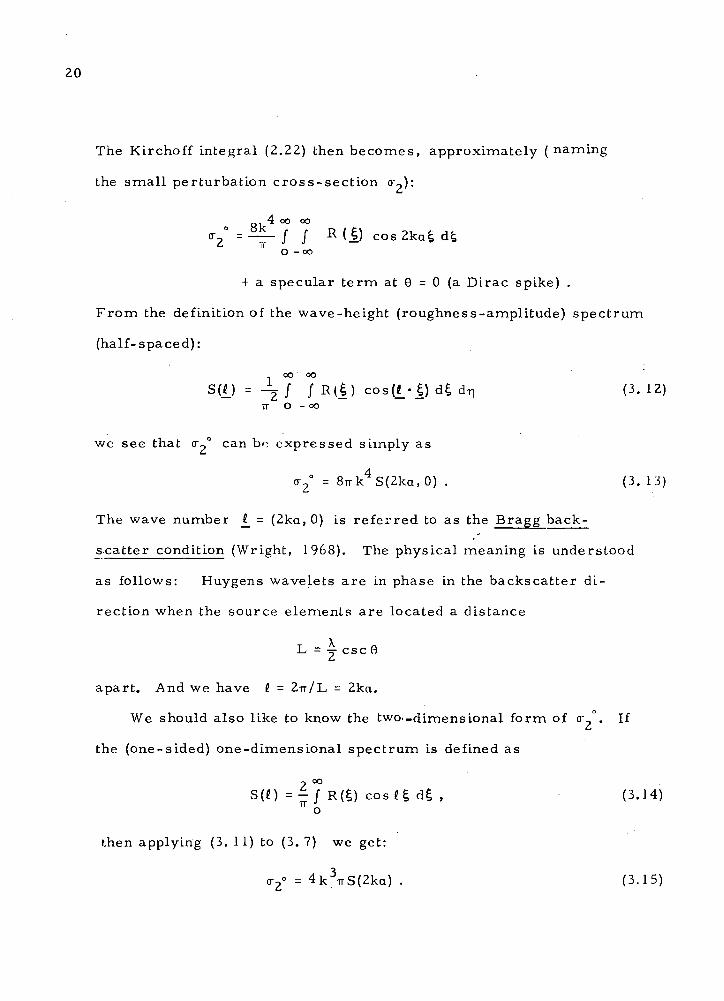
The Kirchoff integral (2.22) then becomes, approximately (naming

the small perturbation cross-section <>•,,):

4 oo oocos

O - oo

+ a specular term at 9 = 0 (a Dirac spike) .

From the definition of the wave-height (roughness-amplitude) spectrum

(half-spaced):

OO OO

TT O - OO

we see that ff~° can bo expressed simply as

cr2° = 8Trk 4 S(2ka ,0) . (3. 13)

The wave number t_ = (2ka, 0) is referred to as the Bragg back-

scatter condition (Wright , 1968). The physical meaning is understood

as follows: Huygens wavelets are in phase in the backscatter di-

rection when the source elements are located a distance

L = j c s c G

apart. And we have (. - 2ir/L = 2ka.

We should also like to know the two>-dimensional form of cr_ . If

the (one-sided) one-dimensional spectrum is defined as

•y OO

-- - / R(£) cos «| d£ , (3.14)

then applying (3. 11) to (3. 7) we get:

= 4k3 irS(2ka) . (3.15)

21

3 . 3 Radar sea-return. The idea of a composite surface.

Chia (1968) appears to be the first to have used a realistic

wave height covariance function in a Kirchoff formulation. What Chia

did, essentially, was to take the equilibrium range spectral law

(Phillips, 1966) and cosine transform to find the covariance function.

The equilibrium range spectral law is (in polar coordinates):

S(K,cp ) = AK'^F(cp) (3.16)

where A is a universal constant and F is a dimensionless spreading

factor normalized so that

ZTT

/ F(cp) dcp = 1 . •o

The equilibrium range is supposed to exist in a fully aroused sea be-

tween wave numbers near the spectral peak down to wave numbers

approaching the capillary-wave regime. Assume that isotropic

conditions prevail, and that the spectrum can be defined by

A 4S ( K ) = £ K ' * , (3.1?)

where K is a low wave number near the spectral peak,

KQ ~ g/U2 ; (3.18)

where g is the acceleration of gravity and U is the wind speed at

a nominal anemometer height.

For microwaves, the propagation constant k is several

orders of magnitude larger than K . Scattering is determined pri-

marily by the wave structure in a wave number domain centered about

22

the Bragg backscatter condition, K = 2ka. This allows a simple ap-

proximation to the covariance function corresponding to (3.17). For small

lags KQr « 1 r - J t,2 + r,2 :

00 TT/2

R ( r ) = - / / K cos(Kr coscp)dK dcp

2~ <r + A ^-(-1 + Y + in K r / 2 ) . (3.19)

where y ~ 0.577. . . is Euler's number.

Since the high-frequency portion of the wave spectrum

is always nearly isotropic, a one -dimensional counterpart to (3.16)

can only be a fictitious analog. However, if one imagines all the

wave energy to be concentrated into one direction, then F = 6(cp),

a Dirac spike, and the one -dimensional spectrum becomes

S(K) = AK~ 3 . (3.20)

The approximation to the covariance function for small lags,

KQi « 1, is

00 oR(|) = A / K cosK£-d|

Ko

2 £2 3~ <r + A-|- (- -j-+ Y + l n K Q S ) (3.21)

It is possible that funnelling all the wave energy into one

direction might produce an unrealistically large amount of scattering

(i.e. , in the two-dimensional approximation to the three-dimensional

scattering problem). Let us allow for a variation of the spectral

constant A by imagining that only a certain band of directions A$

*Luke, Y. L. , Integrals of Bessel Functions, McGraw-Hill, 1962, p. 48.

23

are funnelled into the one direction, that is, let A -*——A. IfTT

nothing else, this artifice will let us see the variation of <r° with a-i-

changing spectral constant.'

Figure 3 shows the two-dimensional Kirchoff solution

(eq. (3.7)) using the covariance function given by eq. (3.21). Nominal

-3 -1values of A = 5 x 10 , U = 15 m sec and X (radar) = IT cm were

u sed in the calculation. The effect of varying the low wave number

cutoif is small (on the order of a few decibels for wind speeds between

5 and 20 m sec ) and is not illustrated. The effect of increasing

wind speed is simply to cause a greater "tilting" of the small wave

structure (which is primarily responsible for the scattering) by the

larger waves. The result is a "smearing" of the incoherent scattered

power pattern. Also not shown is the frequency dependence of the re-

turn. The frequency dependence can be expected to be small. This

follows from the k-independence of both stationary phase and small

perturbation approximations. (Note that k S(2ka) is k-independent

for the K spectrum. )

A comparison of stationary phase and small perturbation

approximations with the Kirchoff integral is made in Figure 4. A

value of o- = 0.215 was chosen to match cr ° with the Kirchoff or0

x 1

at vertical incidence.

»t.

''"The spectral constant is wind-speed dependent. The observations of Ley-kin and Rosenberg (1970), for example, show that A increaseswith wind speed until for high wind speeds A levels off andapproaches its asymptotic (equilibrium) value.

24

Om

<n^ <uO o>"tf •-o»

o>

CD

O o>ro u

c:

oc

0°OJ o>

O

I

OCMI

>

n ro to ft

82

fe -H

n) 43 ̂ 2_< 3 j -i-l

f 13 S

M • Oflco -jj

rt <D i h

C -O 0)is >

««73ani

rt <J

CO T3

a(U .C -

s>*

CO

ooh

^ OO O

„.

s. sCO 3.,., Qi

C ro

-2 «

25

The coincidence of the small perturbation approximation

(<r7°) with the Kirchoff curve provides a validation of small perturb-

ation theory for sea-return from larger incidence angles.

The basic idea behind various "composite surface" models

(e.g., Semyonov, 1966; Fung and Chan, 1969; Krishen, 1971) is illus-

trated in Fig. 5. The backscattered power from small perturbation

and geometrical optics regimes is added incoherently,

°"0 = V + a2° ' (3'22)

where the specular (near vertical) portion of <r ° is suppressed. A

remarkably close agreement with the full Kirchoff integral is achieved.

26

*IO

oc

-20

10 20 30 40Angle of Incident* 0 in D«grte»

50 60

Fig. 4, Stationary phase and small perturbation approximations tothe Kirchoff integral. The Kirchoff solution is the same ascurve 'a' in Fig. 3. aj and 0*2 are respectively given byeqs. (3.8) and (3.15).

*IOr

S.,0

-20

J L J l_ J L10 20 30 40

Angle of Incidence B in Degrees50 60

Fig. 5. The "composite surface" solution as a sum of stationaryphase and small perturbation cross sections.

27

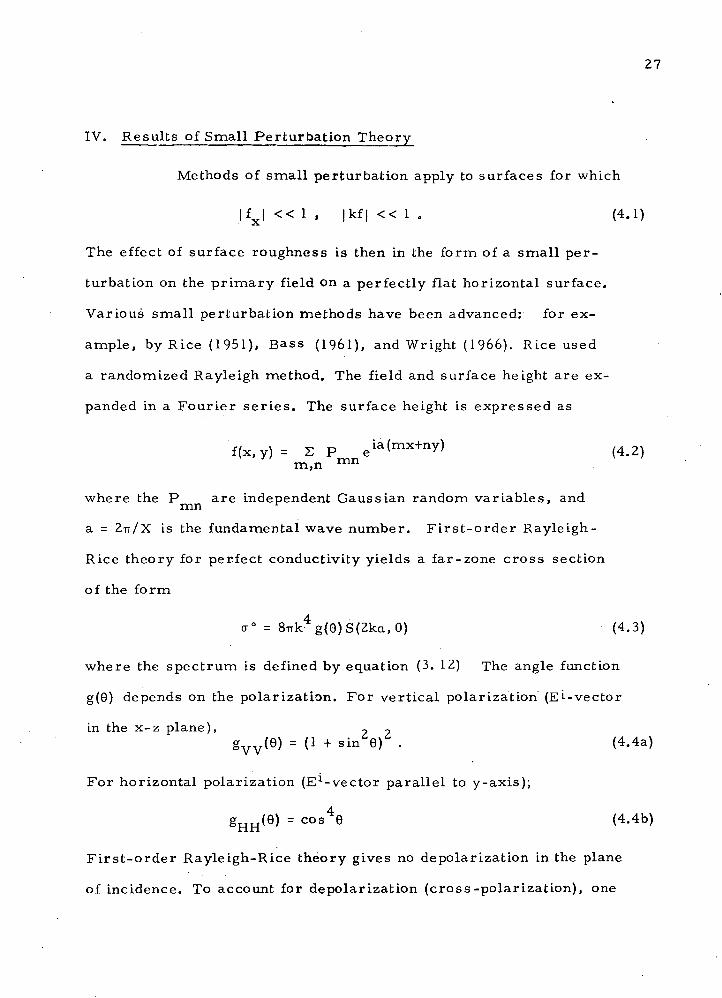
IV. Results of Small Perturbation Theory

Methods of small perturbation apply to surfaces for whLch

| fx l « 1 , |kf | « 1 „ (4.1)

The effect of surface roughness is then in the form of a small per-

turbation on the primary field on a perfectly flat horizontal surface.

Various small perturbation methods have been advanced: for ex-

ample, by Rice (1951), Bass (1961), and Wright (1966). Rice used

a randomized Rayleigh method. The field and surface height are ex-

panded in a Fourier series. The surface height is expressed as

f(x,y) =m,n rnn

•where the P are independent Gaussian random variables, andmn r

a - 2-rr/X is the fundamental wave number. First-order RayleLgh-

Rice theory for perfect conductivity yields a far-zone cross section

of the form

er° = 8irk4g(9)S(2ka,0) (4.3)

where the spectrum is defined by equation (3. 12) The angle function

g(0) depends on the polarization. For vertical polarization (Ei--vector

Ln the x-z plane),gyv(9) = (1 + s ine r • (4-4a)

For horizontal polarization (E1-vector parallel to y-axis);

gHH(9) = cos46 (4.4b)

First-order Rayleigh-Rice theory gives no depolarization in the plane

of incidence. To account for depolarization (cross -polarization), one

28

one must go to second order in the ordering parameters |kf | and

|f |. This has been done by Valenzuela (1967). Fig. 6 comparesx'

the Kirchoff and Rayleigh-Rice solutions for the surface described

by the K spectrum.

.29

V)

Q)jQ

'oO

c

0

b

- 10

-20

.30

5 x IO"3

vv

I

10 20 30 40 50 60A n g l e of I n c i d e n c e 8 in Degrees

M

X)

'o

oc

+ 10

-10

b -20

-30

A« 1.25 x IO"3

JHH.

0 10 20 30 40 50 60Angle of Incidence 9 in Degrees

Fig. 6. First-order Rayleigh-Rice solution. The solid curves"a1 and 'c1 are the same Kirchoff curves shown inFig. 3.

30

V. A High-Frequency Correction to the Kirchoff Approximation

A simple correction to the Kirchoff approximation that

accounts for the effect of surface curvature can be extracted from a

field integral equation. For a perfectly conducting surface free from

singular curves (cusps), the integral equation for the magnetic

field is (e.g., Fock(1945)):

J = J(o) + n X ~ \ J* x V'G dS' (5.1)—s —s 2-n J —s v 'So

where J = n X H is the surface current density and H Is the__g __ _»_

magnetic field on the surface; where:

J_* ' = n X 2H is the Kirchoff value of the current density,

n is the unit surface normal directed outward from the

conducting volume,

H is the incident magnetic field,

( ' ) (prime) denotes source point coordinates x1 as opposed

to field point coordinates, x ,

G = exp(-ik| x - x1 | ) / ]x - x'| is the Green's function for

homogeneous space.

The assumption of a first-order continuous surface is con-

sistent with high frequency approximation we shall be making.

That is, as with the Kirchoff approximation, we shall require gentle

curvature (X/r « 1). Mittra ;': has derived a set of field integral

equations which are valid for surfaces possessing sharp edges.

These equations may provide a basis for future research. The

*Mittra, R. A. J. : Notes for a course given at the University ofIllinois, Department of Electrical Engineering (unpublished).

31

formulation (5.1) is ideally suited to near-planar or smooth geometries.

For, when the surface is locally nearly flat or nearly planar, the inte-

gral contribution is small compare'd to the Kirchoff value n X 2H and

can be regarded as a "small perturbation" on the Kirchoff value. This

is seen from the fact that the vector J_ X V'G is oriented nearly

parallel to the field point normal n, so that the cross-product

n X P X V'G is small.

Fock (1945) has examined the conditions under which a

perfect conductivity formulation is valid. An assumption of perfect

conductivity is strictly justifiable only when the radius of curvature

is large compared to the skin depth (depth of penetration of the field).

Conduction currents can then be considered to be confined to a thin

skin layer, and can then be represented by a surface current density.

Thus, we must have

6 « rc

where 6 is the skin depth (normal to a flat interface), the depth at

which the field has attenuated by a factor of e~ . For all microwave

frequencies up to and including X-band (3 cm), sea water is a good

conductor in the sense that the skin depth is much smaller than the•tf

wavelength. Even at X-band, 6 is small: 6/X ~ l/2ir. Thus, a

perfect conductivity formulation of the integral equation is consistent

with the high-frequency (small X/r ) approximation we are making.

We develop the integral equation for the horizontal rough

surface, z = f(x, y). We use the following notation:

:'Trom Saxton and Lane's (1952) data.

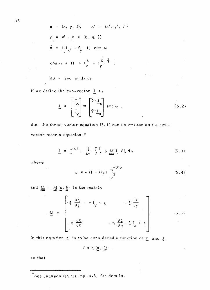
32x = (x, y, f), x' = (x1, y', r

p = x1 - x = (£, TI, £)

n = (-f , - f , ] ) cosx y

2 2 -cos w = (1 + f + f ) *

x y

dS = sec w dx dy

If we define the two-vector J as

J =x- J

y - Jsec ( 5 . 2 )

then the three-vector equation (5. 1) can he written as lV ,o two-

vector matrix equation, *

J = J ( 0 ) + -^- \ ty M J1 d dm— ~ 2ir ,3

where-ikp

+ i k p ) —

( 5 . 3 )

(5.4)

and M = M (x; ^) is the matrix

M = ( 5 . 5 )

In this notation t. is to be considered a function of x and

so that

See Jackson ( 1 9 7 1 ) , pp. 4-8, for details.

33

and

. = f -f8x x x

(x - y)

- y) -

The J component follows from the condition that J_ is tangential

to the surface:

J = f J + f Jz xx y y (5.6)

We relax the high frequency (small curvature) condition of

the Kirchoff approximation to allow for some degree of curvature.

Since we are still dealing with a "smooth" surface, we can assume

the surface height f has a Taylor series expansion about every point,

2 2—o

f(x) = f + f u + f v + f rx— x y xx L f uv + f -xy yy 2

From now on it will be understood that f and the derivatives are to

be evaluated at the local origin x . We shall have u = (u ,v) stand

for the relative (horizontal) position vector of a field point. The

relative position vector of a source point shall be given by

If we form the difference £ = f - f we get

>2 2

x^' - x = u. + _£

= fxf r|y '

A l i t t le algebra will show that the matrix M has the expansion

,2 2

M = M (x;

_ f _+ f 3xx 2 yy 2

-f g . fxy yy

f - - fxx 2 yy 2

(5.7)

34

Thus, to a first approximation, M is independent of the local field

point coordinates 11 and can be expressed in terms of the separation

vector ^ alone. Call this approximation M .

A f irs t approximation to \\> is obtained by letting p cor-

respond to the distance on the x tangent plane,

p = PI -(a2!2 + b2nV (5.8)

where

a2 = 1 + fx2 , b2 = 1 + f y

2 . (5.9)

If we let

* =* = -(1 + ikP l) (5.10)Pi

the leading error term is proportional to the curvature.

If the approximation 4>M = 4" M i-s made the leading

error term is proportional to third derivatives of surface height and

the product of two second derivatives. What we are going to assume

is that the bulk of the integral //^ M \J' d£ dr^ is formed in the

neighborhood of x where the error terms are small. This as-

sumption is difficult to justify. Cullen (1958) has examined the high

frequency behavior of the integral equation (5.1) for a convex body.

There Is an apparent contradiction In the relative importance of the

source distribution near and removed from the field point. We will

see this when we compare the radiative ( far-source) contribution

to the inductive (near-source) contribution to the integral (see below,

p. 39 ). We should expect the mild curvature res t r ic t ion on this

approximation to be very similar to the cri teria (inequalities (2. 7))

35

for the Kirchoff approximation, except that this approximation should

2 2be good to O(\ /r ) rather than O(\/rc) .

In any event, assuming \\>M = fy M , the integral

equation (5.3) becomes

J(u) = J (D)(u) + . / / 4 ' ( 1 ) ( p ) M ( 2 ) ( ) J ( . u + ) d | d T ! (5.11)

Equation (5.11) can be solved exactly by Fourier transformation techni-

ques. Fourier transformation is now a common method for solving

two-dimensional (plane) diffraction problems, where integral equa-

tions of this type occur (Bouwkamp, 1954). But, remember, unlike

a true two-dimensional equation, eq. (5.11) is only approximately

correct. The older method of iterated kernels is a more appropriate

method of solution.

The integral operation takes an O(l) quantity into an

O(X/r ) quantity; and O(X/r ) quantity into an O(\ /r ) quantity,c c c

and so on. Since J_ differs from J/' by an O(X/r ) quantity, we

can set

J = J ( 0 ) + J(1) (5.12)

where J = O(l) (for a unit magnetic field) and _J ' - O( \ f r ).**"~ ~

( 1 ) .Equation (5.11) then yields for J

)(Pl)M(2)(i) J ( o )(u+|)d| dn + o(\2/rc2) .

We have really lost nothing here since equation (5.11) was accurate

only to O(\/r ) to start with. Note that the above equation is

most accurate at the local origin u. And since we no longer need

36

the convolution properties of the original equation because J_ is

a known function, all we need calculate is

^ J^d ld r , (5.13)

For a plane-wave incident field with unit magnetic vector,

has the form

J(°> = 2A e - ' Y (5.14)

where for vertical polarization (E -vector in the x-z plane):

(5.15a)0

and for horizontal polarization (E -vector parallel to the y-axis):

(5.15b)

It is entirely consistent with the development of equation (5.13) to

expand J/ in terms of £ about x neglecting terms of O(X/ r ).

We can do this because when multiplied by the kernel , O ( X / r )

2 2terms become O(X /r ) terms. We then have approximately

T(°) T A -ik(ax-vf) - it. • £ ,r i /: \;r ' = 2A_e x ' • e — (5.16)

where A is equal to (5.15) with f and f evaluated at the localx y

origin, x. (The sub-zero notation is abandoned.) And l_ is

the wave number,

« = k(a - vf , -vf ) (5.17)_ l ' x ' y' * '

Putting ^T in the integral (5.13) we get

(5.18)

37

where .S. is the Fourier integral,

oo.e — — (5.19)

-00

The infinite limits have been applied just to make the integral definite.

The evaluation of this integral is given in the Appendix.

The elements S.. of S are found to be:

f ? f -i

•'2 '^-1

11 2kabv3

kabv

. xx' m )~ -

J

t* J- •• i -kabv

xxIF

(5.20)

where we have defined

and

(a - yf )/a , m = -yf /b

2 2v = (i - r - m

(5.21)

(5.22)

and where again we have

a2 = 1 + f 2

xb2 = 1 + f 2 .

y

The wave numbers kf and km are the projections of the propa-

gation vector k, onto the tangent plane in the x and y directions

respectively. The quantity v is a bit difficult to interpret , but it

can be wri t ten in terms of the "tilt angles" of the surface, defined

by tan iL = f and tan 6 = f :r T x y

38

v2 = cos2(9 - 40 -,cos29 sin26 (5.23)

At (locally) normal incidence, *\i = Q and 6 = 0 so that v = 1

(its maximum value). For local incidence near grazing (i j j = 9 - i r /2 )

v may go to zero causing S to blow up. Since S must.be small if

it is to be a good approximation, large incidence angles must be

avoided.

The correction S, , is seen to be identical to an asymp-

totic form found by Fock (1945) for the current distribution on a

convex paraboloid of revolution. Fock did not use the integral

equation, but rather solved Maxwell's equations by separation of

variables. Fock's asymptotic form holds for large distances away

from the shadow boundary.

Jackson (1971) has shown that the corrected current density

J" + J corresponds with Rice's current density in the case of

gentle curvature and moderate incidence angles.

It is interesting to compare the. criteria (inequalities (2.7))

with our correction. For the one-dimensional case, f = f(x) , alone,

say, the condition that S be small gives

« 1 .•» 3 32kv a

Or, since | f | /a = r ~. , v = cos(0 - \\i) = cos 0' , this means that

cosV » X (5.24)

Note that S is purely imaginary in number. This means

that the perturbed current density _j' ' is 90° out of phase wi th the

zeroth-order current . Exactly how this phase shift will

39

determine the scattered field will depend on the height-curvature cor-

relation properties of the surface.

Returning to the point made earlier, that there is an ap-

parent contradiction in the integral equation between the local nature

of the high frequency approximation and the importance of far- source

contributions, we examine the integral S (see the Appendix). The

inductive contribution comes from the integrals

oo -ikpInd. = / J (Lp^e dPj , n = 0, 2

o

and the radiative contribution comes from the integrals,

,Rad-- / ikp, J ( L p , ) e dp, , n - 0, 2 .

o

- 2 - 1 - 2The ratio Ind/Rad = Rad = v for n = 0 and 2v + v for n = 2.

'ihus, inductive and radiative contributions are comparable: this

despite an intuition that the inductive component might preponderate.

The rapid increase of the ratio with incidence angle (v oc sec 6)

warns us that far-source contributions are becoming more important,

and that the surface curvature must be increasingly mild if the local

nature of the solution is not to be violated.

To summarize our results, we write the corrected current

density _J as

J = J (0)+J; (1) ~- (I + §)J ( 0 ) (5.25)

where I_ is the identity matrix.

40

VI. Calculation of the Scattered Power

We apply our results to the calculation of the average power

backscattered from a random rough surface. In the case of perfect

conductivity, the far-field Stratton-Chu integral* reduces to:

., -ikR .,-E(R)= i^ e R X //R x(-r|Js secu) e -dxdy. (6.1)

o

E_ is the electric field vector, R = RR is the position vector of the

far field (Fraunhofer zone) point; x is the position vector of the source

points on the surface; A is the illuminated area; and r| is the <

impedance of free space.

For backscatter, the unit vector R is directed toward the

source of incident radiation and so is given by

R = (-Q, 0, v) .

Since in the far field the E-vector oscillates transversely to the propa-

gation vector kR , we have

E -R = 0 ;

hence only two components are needed to specify E. In practice the "

"horizontal" and "vertical" components are used,

EH = Ey

and

V -1E — — v jL .

For a unit incident electric field, we have

'"For example, see Silver (1949), p. 161. The Stratton-Chu integralis a particular vector form of the Helmholtz integral, eq. (2;1).

41

n J s e c

f J + f Ji- x x y y J

and J and J are given by equation (5.25). (We are now assuming a

unit incident electric vector.) Expressing the amplitude vector of

the incident field A explicitly for H and V polarizations, but keeping

the symbols S. . for the elements of S , equation (6.1) yields for the

four polarization combinations:

HH

HV

af )(1 - S, ,) - af £x'v 11' y

- 2 a f ( Y + a f ) S

- (a f

(6.2a)

(6.2b)

(6.2c)

(6.2d)

The f i r s t H or V stands for a horizontally or vertically polarized

incident wave; the second H or V stands for the horizontal or

vertical component of the backscattered wave. In the above, we have

used the fact that S?2 = -Si i > we have let C stand for

-tk exp(- ikR)/2irR .

The scattered power is proportional to | E | . The usual way

ite |E I is to form the twi

The integrals (6.2) are of the form

to calculate |E| is to form the two-fold integral from |E| = E E''" .

4Z

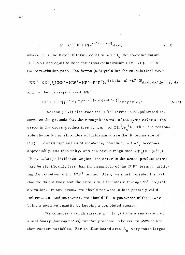
E = C//(K + P)e~ L 2 k ( a X ' Y f ) dxdy (6.3)

where K Is the Kirchoff term, equal to -y + af for co-polarization

( I f H . V V ) and equal to zero for cross-polarization (HV, VH). P is

the perturbation part. The forms (6.3) yield for the co-polarized EE*:

EE*= CC*////(KK' +K1P::: + K P ' + P ' P * ) e " l a x " x " Y " d x d y d x ' d y t ; (6.4a)

and for the cross-polarized EE * :

E E * - C C : : 7 / f / P ' P * e ~ L 2 k ' a ( x ' ~ x ) ~ Y ( f ' ~ f ) J d x d y d x ' d y ' (6.4b)

Jackson (1971) discarded the P'P''~ terms in co-polarized re-

turns on the grounds that their magnitude was of the same order as the

error in the cross-product terms, i.e. , of O(X /r )• This is a reason-

able choice for small angles of incidence where the K terms are of

O( l ) . Toward high angles of incidence, however, y + af becomes

appreciably less than unity, and can have a magnitude O(f ) = O ( X / r ).X C

Thus, at l a rge incidence angles the error in the cross-product terms

may be significantly less than the magnitude of the p'p* terms, just i fy-

ing the retention of the p'p'i- terms. Also, we must consider the fact

that we do not know how the errors will transform through the integral

operation. In any event, we should not want to lose possibly valid

information, and moreover, we should like a guarantee of the power

being a positive quantity by keeping a completed square.

We consider a rough surface z = f(x, y) to be a realization of

a stationary (homogeneous) random process. The return powers are

then random variables. For an illuminated area A very much larger

43than the scale of roughness, one might expect the variability in return

power to be small. However, this ignores the fact that scattered

radiation from different portions of A will have random relative phases,

resulting with Rayleigh-type statistics of signal fading and reinforce-

ment. To calculate the average power we proceed by taking an ensemble

average or expectation of all possible surface realizations, denoted by

corner brackets ( • • • ) > • Since expectation and integral operations are

commutative, the average power return in (6. 4a) can be written as

< | E | 2 ) = CC*J7J7<K'K+ K'P*+ KP' + P'P*) •

i2kv(f ' - f ) . -iZka(x'-x) , , - , , • , ,t • e Y )e dxdy dx1 dy1 ,

and similarly for (6.4b).

An Immediate consequence of stationarlty Is -that expectations

of the type

can be expressed as

«(

where

*=

and

The expectations are computed on the assumption that f is a

stationary Gaussian random process of zero mean, (f) = 0. Define

the twelve dimensional random vector ^Y whose f i rs t six elements

are f, f , f , f , f , f and whose second six elements arex y xx xy yy

f, f ', etc. The mean of any derivative of a stationary process Is•5C

zero; hence

44

CY > = o .

Since the mean of the vector is zero the covariance matrix y\ can

be wri t ten as

The multivariate Gaussian distribution with the covariance /V has

the probability density function,

1 f .1 T .-1

T 1where y is the transpose of y_ and A~ is the inverse of A- Define

the characteristic function of ^Y ,

(6.8a)

(6.8b)- oo - oo - oo

If p(y_) is the multivariate normal distr ibution (6.7), then g> has the

f o r :m''":

f 1 T 1( { > ( t ) - exp -<- ~2 t_ A_£ r •

Or, in terms of elements t. ,

y (t,, t2> • • • , t12) = exp J- -j T \ . . t . t . L (6.9)

Now, the required expectations can be generated in a simple

manner from the characterist ic function by expressing the slope-

dependent coefficients in S as polynomials in f and f . We expand

the (three) slope-coefficients in (5.20) in a Taylor series about

*E. g. , Wilkg (1962) , p. 168.

45

f = f . = 0. (Expansion about the rms values N/TTT , x/TTT might bex y £ £ j ^

more sensible, but it is a good bit more difficult. ) We can truncate at

f i rs t , second, or third order in slope. With the multipliers of the

phasor e x p { i 2 k y ( f ' - f)} expressed as polynomials in the Y-elements

we can compute term by term the expectations of the forms:

( e i2k v (Y 7 -Yi) )

. i2kv(Y -YJ(Y p e } (6.10)

i2kY(Y -Y )

These averages are computed from the characteristic function in the

manner outlined: Define the twelve dimensional vector t_''" (star does

not mean complex conjugate) all of whose elements are zero except for

t '" and t^'f which have the values,

t , * = -2kV1 (6.11)

The expectations (6.10) can then be wri t ten as

/ ' \(e- — >

<v -* -

From the definit ion of the characteristic function (6.8), we find

46

-I-, it • Y s A / i -* \(e - — ) = <f>(t_ )

atp t = t*

Y e [ t-"'Z\ - j2

p V > t = f(6.12)

From (6.9) and the definition of t* (6.11) we find

,n - x 1 7 ) }

at atp q

at

•=[^-Xql+V(-V + V(6.13)

In the manner outlined, the required expectations can be

calculated. The last step is to find the covariances X. . . as a functionij

of the lag ^ = x1 - x. All 72 covariances can be expressed as partial

derivatives of the covariance function,

In accordance with our "smoothness" condition, R(£) possesses con-

tinuous partial derivatives of all orders.

If the illuminated area A is large compared to the scales

of roughness in the x and y directions ("correlation lengths"), then

the scattering integrals of the form

47

- i2ka(x'-x) , , - , , - . .v ' dxdydx'dy' ,

are nearly equal to

, r r* t t - \ - a , t ,/ / - ^- OO - I

C(|) stands for the expectation ( { • • • } e ^ ) and Y is a large

distance in the r\ direction. Because ot the behavior ot the exponential

$ , Y can go to infinity only in the sense of the limit

oo Ylim / / C(|)eY— oo -oo -Y

and it is in this limiting sense that the inlinite limits ot integration

in the final formulas have been applied.'"

The power returns are usually given in terms 01 the normal-

ized isotropic radar backscatter cross sections, <r° , defined by

< | E | ) is the quantity we have calculated, namely, the ratio of

( |E | ) at the receiver to |E| incident. Here, we do not consider

realistic antenna gain patterns. The incident field is taken to be of

•Xr O-

constant amplitude over the area A .'r''~

Cf. pp. 13, 14.

"-Requiring the incident field to be of constant amplitude is only anartificial restriction. The cross-section is really determined bythe statistical structure of a small patch, over which the antennagain pattern is practically constant. The effect of gain patterncan be accounted for formally by introducing an effective areaA in place of A .e r o

48

Following are the scattering integrals arrived at. The co-

polarized returns are expressed as

°~HH ~ K + P + s

(6.14)cr^v = K - P + S

where K represents the "Kirchoff" part , P the "perturbation" part,

and S represents the perturbation "squared". The P-term Is calcu-

lated to-second order In slope, and the S-term is calculated to zeroth

order in slope. To f i rs t order in slope, the cross-polarized returns

are equal:

where D stands for "depolarized" return. As previously defined,

B stands for

B = - R ( 0 ) + R ( £ ) ;

we introduce the additional symbols:

B i e = -Ru(-] + Ru(^ ' 'e tc-

We find, then, that:

49

2oo ooK =

O - oo

[4ka(ReBe |- Z R

cos

B(16b)

2 oo oo

o - oo

-2 -4

2 2B )

2 2,; \ I

( I6c )

2 oo ooCTVx ~

cos

(I6d)

50

The Kirchoff term is in the form used by Chia (1968). Beck-

mann'-s form, eq. (2.22), differs because of the integration by parts

and the neglect of edge terms. The K-term can be integrated by

parts, yielding Beckmann's form upon neglecting "edge terms". For

most practical applications, we have deep fade conditions, 2k-ycr » 1,

and a large A . One need only be careful of edge effects when

• numerically computing the integral for large angles approaching

grazing incidence (this would entail having to carry the integration

over a larger lag).

51

VII. Properties of the Solution

Here we examine the general nature of the solution, give

a sample calculation, and present for comparison some published sea-

return data.

7.1 Comparison with the results of f i rs t -order jlayleigh-Rice theory

It was shown in section 3.3 that for values of the spectral

constant A typical of the sea, the small perturbation approximation be-

comes very accurate toward large incidence angles. This fact demon-

strates the validity of small-perturbation methods for sea-return from

angles of incidence exceeding 9 = 45° or so. We should like to compare

our solution with Rayleigh-Rice theory for the condition of small rough-

ness amplitude ( i .e . , for Zk^cr « 1). If we linearize the integrands of

the scattering integrals (6.16) and integrate using the definition of the

spectrum (eq. (3.12) ), we get scattering cross-sections of the form:

cr° = 8Trk4g(9)S(2ka,0)

where

gHH(9) = <1

gvv(8) = (l+tan29)2 (

and the depolarized return is zero. Comparing this with Rice's

g(9), eqs. (4.4 ), viz. ,

4 2 2gHH(9) = cos 6 = (1 - sin 9)

gvv(9) = (1 + sin29)2

we see that (7.1) is in good agreement for 9 ~30° . The failure to

52

match Rice 's g(0) for large incidence angles indicates a general failure

of our solution for representing backscatter from any surface having an

appreciable spectral density at the first-order Bragg condition (K = 2ka)

> °for 9 ~ 40 . Clearly, the simple curvature correction is over-predicting

the splitting of the copolarized returns from these angles. The failure

of representation at large angles is not surprising, and could have been

expected on the basis of the criterion (5.24) .

'' ' -47. 2 A sample calculation: Copolarized returns from, an isotropic K •

spectral-law surface and a one-dimensional K~ j spectral-law surface

We should like to apply our formulas to scattering from an iso-

_4tropic surface described by the simple K spectral law (eq. (3. 17) ) .

-4It is understood that a K law surface is extremely rough (having

firs t -order discontinuities) and poorly conforms with our requirements

-4of smoothness. However, as the K law spectrum is a simple and

realistic descriptor of the sea surface, we shall use it.

-4Assume that the K law is valid for wave numbers in the re-

gion of the Bragg condition K = 2ka. The detailed behavior of the

spectrum for wave numbers much smaller than or much larger than the

Bragg wave number little affects the scattering. As in section 3.3

we take a low wave number cutoff K corresponding to the spectral

peak (cf. eq. (3. 18)). The covariance function is very well approxi-

mated by eq. (3. 19). Now, the second derivatives of the covariance

function diverge logarithmically at the origin. As far as the problem

of computing the scattering integrals is concerned, we can get around

53

this mathematical difficulty. We can impose a high-frequency spectral

cutoff, K = K , say, corresponding to a viscous cutoff. Cutting off

the spectrum abruptly this way creates a high frequency oscillation

near the origin which is entirely artificial. Rather than doing this,

it is simpler (and more sensible) j.ust to "cut out" a small lag region

near the origin, r $r , in which the second derivatives are to be

taken as constant. Thus, we define for r <r

2 r 9^* s '

where cr is the slope variance. In terms of a high frequencys

spectral cutoff, cr would be given by

2 K

o

From the definition of the covariance function (eq. (3.19)), viz. ,

2 2

R(r) = cr + A ~ (-1 + Y + In K r /2 ) (7.4)

it is seen that r relates to the cutoff K asv v

r = 2(K e7)"1 (7.5)V * V '

We consider only the zeroth order slope terms in the P-integral.

On transforming the Kirchoff integral and the f i rs t two terms of the

P-integral to polar coordinates (r ,c />) and integrating over <j> , we

find | using the above definitions):

54

= K ± P

K = 2k2Y~2 J Jo(2kar)e4k ^ B r dr

o

CO ? ?

2 i. 2 r 4V v KP = 2k A J a ^n — J (2kar)e r rdr (7 .6)

°

Figure 7 shows the copolarized returns given by the integrals

(7.6) . The values of the constants used are: A = 4.05 x 10 (from the

Pierson and Moskowdtz'" frequency spectrum with A = a/2) ; wind speed

U = 7 . 5 msec ; k = 2 cm (X-band); K =20 cm (a nominal value of the

viscous cutoff). In the isotropic case, the perturbation (P-term) is

zero at vertical incidence, as we can see by putting a = 0 in (7 .6) . The

failure of the solution at angles approaching 9 = 45° is seen in the rapid

falling away of the horizontally polarized returns as K + P goes to

zero. This failure occurs in the manner described by the linearized

solution (eqs. (7.1)) which gives a gr r r r&S' ) = 0.riri

A similar treatment can be given to the two-dimensional scatter-

ing analog. In the two-dimensional case, the covariance function is

given by eq. (3.21), and Btt is defined to be

° • 6*evA {7>7)

*In Neumann and Pierson (1966), pp. 349-352.

55

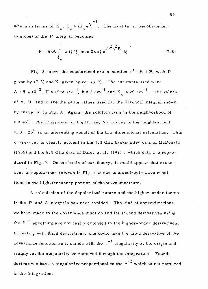
-1in terms of K , £ = (K e ) . The f irst term (zeroth-order

v v v

in slope) of the P-integral becomes

CO

P = 4kA )' ln (£ /£ )cos 2ka£ e4 k Y B d£ (7 .8 )

v

Fig. 8 shows the copolarized cross-section, <r° = K _+ P, with P

given by ( 7 . 8 ) and K given by eq. (3. 7). The constants used were

A = 5 X ]0~ , U = )5m sec"1, k = 2 cm"1 and K =20 cm"1 . The valuesv

of A, U, and k are the same values used for the Kirchoff integral shown

by curve 'a' in Fig. 3. Again, the solution fails in the neighborhood of

0 = 45 . The crass-over of the HH and VV curves in the neighborhood

O

of 9 = 20 is an interesting result of the two-dimensional calculation. This

cross-over is clearly evident in the 1.3 GHz backscatter data of McDonald

(1956) and the 8. 9 GHz data of Daley et al. ( 1 9 7 1 ) , which data are repro-

duced in Fig. 9. On the basis of our theory, it would appear that cross-

over in copolarized returns in Fig. 9 is due to anisotropic wave condi-

tions in the high-frequency portion of the wave spectrum.

A calculation of the depolarized return and the higher-order terms

in the P and S integrals has been avoided. The kind of approximations

we have made to the covariance function and its second derivatives using

-4the K spectrum are not easily extended to the higher-order derivatives.

In dealing with third derivatives, one could take the third derivative of the

covariance function as it stands with the r singularity at the origin and

simply let the singularity be removed through the integration. Fourth

derivatives have a singularity proportional to the r which is not removed

in the integration.

56

o1-1

(Hnti— iOa-ooIH

.8

ao

oa

£ <oo o•^ J5y ««

^ S—4 9

a) nt

o oO 0)

.2 •

0) O

S »4a.

<I>>H

X

H

•r~

•bO

57

8

Oin

(AoO

O

•*-

OCVJI

oroi

Ot-i

0)

fia.u4)t-i

0)N

OO.OO

,-» o °O 2 w

fO fl« «M

O y

c .iJ

O <ut3

w G)

0» Mc p

«fl

§•3._! flj

-O hI -"

oo

s| m 0 -o

58

toCIH

T34)N

• •4

tHrt

<-H

8-ou

0)

oI01<Q

so

_ rt

t,0).LJ•Urtu

PiR)DU

O

59

A detailed analysis of how the scattering integrals might be

"best applied" to the radar sea-return problem is outside the scope

of this work. For X-band radar sea return, an accurate spectral

representation of the high-frequency gravity and capillary waves in-

cluding a viscous cutoff is one possibility. Then, all required deri-

vatives of the covariance function will exist and the scattering integrals

could then be computed. For lower-frequency microwaves, a detailed

modelling of the covariance function near the origin is not necessary.

But it remains a problem how to control most reasonably the behavior

of the higher-order derivatives near the origin. We see that the

practical problem of using the scattering integrals is intimately linked

with the problem of error in this high-frequency approximation to the

scattering problem.

60

VIII. Discussion and Conclusions to be Drawn

A few years ago, Prof. R. K. Moore pointed out the need for

extending KLrchoff techniques beyond the tangent-plane approximation.*

With the curvature correction to the tangent-plane approximation,

this has in a good measure been accomplished.

The sample calculations illustrate the potential strength of

this "corrected Kirchoff theory" for predicting radar sea-return from

the near-vertical (specular regime) and from the transition region

between specular and diffraction regimes. Because of the greater

analysis needed to reasonably model the fourth-order mixed partial

derivative in the depolarized scattering integral, no sample calcu-

lation has been given. A calculation of the depolarized signal should

prove most interesting, for it is not masked by the large specular

component as the copolarized signals are. As the depolarized return

depends essentially on the nonlinear component of the source distri-

bution, this scattering solution is in apeculiarly good position to

model depolarization near the vertical. Comparison with the second-

order Rayleigh-Rice solution will provide a basis for testing the two

solutions over the full range of incidence angles.

On entering the pure diffraction regime the solution deterior-

ates rapidly due to the over-emphasis on curvature effects and the

increasing importance of non-local diffraction processes. It is interest-

ing to note that the tangent-plane approximation alone provides more

*In his paper "Scattering from Rough Surfaces" delivered to the Aug.1969 General Assembly of the URSI, Ottawa, Canada.

61

reasonable predictions, although it cannot account for the polari-

zation dependence. The excessive splitting of the copolarized re-

turns at larger angles can be controlled by artificial means, and this

possibility has not been explored. For example, the wave spectrum

could be filtered according to a smoothness criterion in order to re-

move the high frequency waves which contribute to an intolerably

large surface curvature. The derivatives of the covarlance function

corresponding to the "smoothed" surface could then be used in the

scattering integrals. In this way, it would be possible to control the

extent of splitting, and to establish a better correspondence with reality.

This route Is, however, not physically appealing.

Rather than manipulate the solution by artificial means, one

should admit the failure of the solution and recognize that at the

larger incidence angles small-perturbation methods become applicable.

If the Rayleigh-Rice solution shown in Fig. 6 is compared with the

corrected Kirchoff. solution, Fig. 8 , there is seen a fairly con-

tinuous transition between the two solutions in the neighborhood of

45 degrees. The idea of forming a "composite" solution suggests it-

self. If or ° represents the high-frequency cross-section and cr°

•J,

represents the low-frequency cross section,'1" then a continuous

solution for all incidence angles might be obtained from a weighted

addition of the two cross sections: for example,

* Here tr ° might be calculated to first-order in slope, and correctedfor finite conductivity by the relationship, eq. (3.9 .).. The smallperturbation cross-section might be a f irst- or second-order.Rayleigh-Rice solution for finite conductivity, possibly includingthe ar t i f ice of mean-plane tilting (Valenzuela, 1968; Guinard etal. , 1971).

62

cr = W(e)<r1° + (1 - W(6))o-2° •

The weighting function W would be near unity for small angles and

fall fairly rapidly to near zero at some critical angle in the neighbor-

hood of 45 degrees. The complementary weighting of the two cross-

sections guarantees that if both cross-sections were identical (say,

were both perfect solutions), then we should have cr° - cr ° = cr ° ,

From the standpoint of electromagnetic theory, it appears that

between the high-frequency and small-, perturbation approximations,

the radar sea-return problem is virtually solved. This is, however,

within the framework of Gaussian surface statistics. Clearly, we are

at a point of theoretical development where a more accurate description

of the sea-surface in terms of its statistical properties is needed. It

seems to make little sense to calculate the small corrections to the

Kirchoff value near the vertical when the Kirchoff value itself is likely

to be in significant error in its Gaussian form. While the height

distribution of ocean-surface gravity waves is to a very good f irs t ap-

proximation Gaussian, the skewness of the distribution caused by the

nonlinearity of the wave motion becomes increasingly important when

considering slope and curvature distributions, and the joint distri-

butions of these variables. Longuet-Higgins .(1963) in a remarkable

paper has shown how higher-order surface statistics may be de-

rived from the nonlinear hydrodynamical equations of motion for

gravity waves. Longuet-Higgins1 development in terms of character-

istic functions and "cumulants" ties in closely with the methods we

have employed to calculate the statistical averages in the scattering

integrals, and one is tempted to think of a rather effortless extension

63

of KLrchoff techniques to the non-Gaussian solution. The problem

with a transition to noiv-Gaussian statistics is that the deviation from

normality of gravity waves is quite different from the deviation of

capillary waves. For example, gravity waves exhibit a positively

skewed distribution function, while the skewness of capillary waves

can be negative. For decimeter radars,a modelling of gravity waves

alone is possible; but for centimeter radars, both gravity and capil-

lary waves are important, and a simple non-Gaussian model may

be near-impossible to develop.

A current research effort by Prof. W. J. Pierson here at New

York University is aimed at providing a more detailed description of

the high-frequency wave structure in terms of the wave-height spectral

density (Pierson et al. , 1971). Open-ocean measurements of the high-

frequency portion of the wave spectrum (characterized by "chop",

"ripples" and capillary waves) are non-existent, although some statis-

tical information is available (e. g. , the estimates of slope variance

by Cox and Munk (1954)). Hess et al. (1969) have shown that labora-

tory measurements of wind-gene rated waves (conducted in "wind-

wave tunnels") can provide useful information on the open-ocean wave

statistics. Along with certain field observations (e. g. , the near-to-

shore observations of Leykin andRosenberg (1970)) , laboratory

studies are yielding the increased knowledge of the high wave-number

portion of the spectrum necessary for more accurate radar sea-return

predictions.

64

Studies concerned with the effect of surface roughness on the

natural microwave emission characteristics of the sea require the bi-

*static scattering cross-section . In this problem, one is concerned

with an absolute power level, and a relative decibel representation of

the scattered power pattern is inappropriate. The polariza.tion effects

in the near-specular direction will appear small on a logarithmic plot

compared to the polarization effects at large angles from the specular

direction, although the polarization effects (diffraction effects) in the

two regimes are of comparable absolute value. Thus, any effort to ac-

count for pure diffraction processes in the bistatic cross-section must

model these processes in. the near-specular direction, as well as in the

pure diffraction regime at angles far from the specular direction. Since

this corrected Kirchoff theory is particularly suited to the near-specular

regime, an extension of the scattering integrals to the bistatic case should

be considered.

*For a formulation of the natural emission problem, see Stogryn (1967b).

65

REFERENCES

Bass, F. G. , 1961: RadLowave,propagation over statisticallyrough surfaces. (In Russian) Radiofiz. , 4_(3), 476-483.A summary of this work can be found in Bass, F. G. ,I. M. Fuks, A, I. Kalmykov, and A.D. Rosenberg,1968: Very high frequency radiowave scattering by adisturbed sea surface. IEEE Trans. Antennas and Propagat.AP-16, 554-559.

Beckmann, P. and A. Spizzichino, 1963: Scattering of ElectromagneticWaves from Rough Surfaces. Pergamon Press, New York.

Bouwkamp, C. J. , 1954: Diffraction theory. Reports on Progressin Physics, Vol. XVII.

Chia, R. C. , 1968: The theory of radar backscatter from the sea.Center for Research, Inc. Tech. Rpt. 112-1, Univ. of Kansas.

Cox, C. , and W. Munk, 1954: Statistics of the sea surface derivedfrom sun glitter. J. Mar. Res., 13, 198-227.

Cullen, J. A., 1958: Surface currents induced by short-wavelengthradiation. Phys. Rev. , 109, 1863-1867.

Daley, J. C. , J. T. Ransone, Jr., and J. A. Burkett, 1971: Radarsea return - JOSS I. NRL Rpt. 7268, Naval Res. Lab. , Wash. D. C.

Deryugin, L. N. , I960: The reflection of a laterally polarizedplane wave from a surface of rectangular corrugations. ( InRussian)Radiotkhn. 15(2), 15-26. A summary of this work canbe found in Beckmann and Spizzichino, 1963, pp. 59-66(see above).

Felsen, L. B. , 1964: Quasi-optic diffraction. In Quasi-Optics,Microwave Res. Inst. Symposia Ser. Vol. XIV, PolytechnicPress, Brooklyn, New York.

Fock, V. A., 1945: The current distribution induced by a planewave on the surface of a conductor. In ElectromagneticDiffraction and Propagation Problems by V. A. Fock,Pergamon Press, New York, 1965.

Fung, A.K. , and H. L. Chan, 1969: Backscattering of waves bycomposite rough surfaces. IEEE Trans. Antennas andPropagat., AP-17, 590-597.

66

GuLnard, N .W. , J. T. Ransone, and J. C. Daley, 1971: Variationof the NRCS of the sea with increasing roughness.J. Geophys. Res. , 7£, 1525-1338.

Hagfors, T. , 1964: Backscattering from an undulating surface withapplications to radar returns from the moon. J. Geophys.Res., 6_9, 3779-3784.

Hess, G. D. , G. M. Hidy, and E. J. Plate, 1969: Comparison betweenwind waves at sea and in the laboratory. J. Mar. Res. ,27, 216-224.

Jackson, F . C. , 1971: A high frequency correction to the Kirchoffapproximation, with application to rough-surface EMwave scattering. Geophys. Sci. Lab. Tech. Rpt. TR-71-8,New York University.

Katzin, M. , 1957: On the mechanisms of radar sea clutter.Proc. IRE, 45, 44-54.

Kaufman, D.E., 1971: A vector solution for electromagnetic wavescattering from a rough surface of arbitrary dielectricconstant. Radio Sci. , 6^(1), 7-20.

Krishen, K. , 1971; Correlation of radar backscattering cross sectionswith ocean wave height and wind velocity. J. Geophys. Res. ,76_, 6528-6539.

Lenz, R. , 1971: A numerical study of electromagnetic scattering fromocean-like surfaces. Ph.D. Thesis, Unv. of Ohio.

Leykin, LA. and A. D. Rosenberg, 1971: Study of the high frequencypart of the spectrum of an agitated sea. (Transl. of Izv. )Atmos. Ocean Physics, 6^, 1328-1332.

Long, M. W. , 1965: On the polarization and wave length dependenceof radar sea echo. IEEE Trans.. Antennas and Propagat. ,Vol. AP-13, 749-75"4~:

Longuet-Higgins, M.S., 1963: The effect of non-lonearities on statisticaldistributions in the theory of sea waves. J. Fluid Mech. , 17,459-480.

Lynch, R. J. and R. J. Wagner, 1970: Rough surface scattering: shadow-ing, multiple scatter, and energy conservation. J_. Math. Phys. ,11, 3032-3042.

67

MacDonald, F. G. , 1956: The correlation of radar sea clutter onvertical and horizontal polarization with wave height andslope. Conv. Rec." IRE, 4, 29-32..

Meecham, W. C. , 1956: Variation method fo.r the calculation of thedistribution of energy reflected from a periodic surface.J. Appl. Phys. , 27, 361-367.

Moore, R.K. , and W. J. Pierson, Jr., 1971: Worldwide oceanic windand wave predictions using a satellite radar-radiometer.J. Hydronautics, _5, 52-60...

Neumann, G. and W. J. Pierson, Jr.. 1966: .Principles of PhysicalOceanography. Prentice-Hall, Englewood Cliffs, New Jersey.

Phillips, O. M. , 1966: Dynamics of the Upper Ocean. CambridgeUniv. Press, London, pp. 109-115.

Pierson, W. J. , Jr. , F. C. Jackson, R.A. Stacy, and E. Mehr, 1971:Research on the problem of the radar return from a wind-roughened sea. In AAFE Principal Investigators' Review,proc. of a meeting held at NASA/Langley Res. Center, Hampton,Va. , Oct. 5-6, 1971.

Rice, S. O. , 1951: Reflection of electromagnetic waves from slightlyrough surfaces. Commun. Pure and Appl. Math. , 4_, 451-478.

Rouse, J. W. , 1970: An extension of the slope-facet model of radarbackscatter from the sea. Remote Sensing Center, Tech.Rpt. RSC-H, Texas A&M Univ.

Sancer, M. I. , 1969: Shadow-corrected .electromagnetic scatteringfrom a randomly rough surface. IEEE Trans. Antennas andPropagat. , AP-17, 577-584.

Saxton, J. S. and J. A. Lane, 1952: Electrical properties of sea water.Wireless Engineer, 29, 269 (London).

Semyonov, B. I. , 1966: Approximate computation of scattering by roughsurface contours. (Transl. of Izv. ) Eng. and ElectronicPhysics, _U_, 1172-1187.

Silver, S. , 1949: Microwave Antenna Theory and Design. M. I. T.Rad. Lab. Ser. No. 12, McGraw-Hill.

Stogryn, A., 1967a: Electromagnetic scattering from rough finitelyconducting surfaces. Radio Sci. , 2, 415-428.

, 1967b: The apparent temperature of the sea at microwavefrequencies. IEEE Trans. Antennas and Propagat. , AP-15,278-286.

68

Valenzuela, Q.R., 1967: ; Depolarization of EM waves by slightlyrough surfaces. IEEE Trans. Antennas and Propagat.,

' . AP-15,

. , 1968: Scattering of electromagnetic waves from a tiltedslightly sough surface; Radio Sci. , ^, 1057-1066.

Wilks, S. S. , 1 962; Mathematical Statistics. John Wiley and Sons,N e w York." . • ^ - - • • • • r > . • • • < - • • . ' • • • • . - , . • • • • ; • • / • • -

Wright, J. W. , 1966: Backs catte ring. frprn capillary waves with appli-cation to sea clutter. IEEE: Trans. Antennas and Propagat.

" AP-14, 749r.754; V ' ' •

_ , 1968: A new mp del of sea clutter. IEEE Trans. Antennasand Propagat. y;' A F- *6, 21 7-223.

Wright, J. W. and W. Ci Keller, 1971: Doppler spectra in microwave scatteringscattering from wind waves. Phys. Fluid, 14, 466-474.

APPENDIX

Evaluation of an integral

The Fourier integral,

69

(Al)

involves three types of integrals, viz.

J 2 (1 + i kp . ) - i . ( kp + I . J)T) V _1_ o • • 1 - d £ d T) (A2)

On transforming to the elliptical coordinates ( p , , c p ) defined by

... - £ = — cos <P •• •

.T] =T— sin

these integrals become

(A3)

a b I-o o

1 2—2 cos <pa

. 2 ._^ sin 0

2(0 I

-i [kp,+L,p,cos(0-(p)](A4)

70

2 2,2 2

where (A5)

and 0 = tan"(a-

(A6)

Integrating over the polar angle we get

OO

IT \

ab J0

-

<

'jj

a

1

0 _

••W '

— j cos 2©a

~ cos 2©b*

v -£5 Sin2®s

—"

> • J2(Lp1) ikP l)e-ikp,

(A7)

where J and J_, are Bessel functions. Evaluation of the radiationo tL

integrals, i.e., those integrals involving the factor ikp, are a bit

tricky, and are not to be found in standard tables of Fourier/Bessel

transforms. If the substitution s = ik is made, the integrals be-

come formally Laplace transforms which can be found in tables.

We find that

, oo -;sp.ikPl)J (LPl)e 1

vZ) for n = 0

(A8)

for n = 2

71

where v = (1 - L 2 /k 2 ) 2 .

The ratio of radiative to inductive contributions is for n = 0:

RadInd 2 x r2

s + L

-2= v

s=ik

and for n = 2:

RadInd

JLs(2 + s/V s - j.= <i V -f y (A9)

Substituting (A8) into (A7) yields for the forms (A2):

- 2 -rr i

k a b

(1 -

-tm/a b

(A10)

where

and

I = (a - yf /»)

m = - -yf /b

NASA-Langley, 1974

NATIONAL AERONAUTICS AND SPACE ADMINISTRATION

WASHINGTON, D.C. 2OS46

OFFICIAL BUSINESS

PENALTY FOR PRIVATE USE S3OO SPECIAL FOURTH-CLASS RATEBOOK

POSTAGE AND FEES PAIDNATIONAL AERONAUTICS AND

SPACE ADMINISTRATION451

POSTMASTER : If Undeliverable (Section 158Postal Manual) Do Not Return

"The aeronautical and space activities of the United States shall beconducted so as to contribute . . . to the expansion of human knowl-edge of phenomena in the atmosphere and space. The Administrationshall provide for the widest practicable and appropriate disseminationof information concerning its activities and the results thereof."

—NATIONAL AERONAUTICS AND SPACE ACT OF 1958

NASA SCIENTIFIC AND TECHNICAL PUBLICATIONSTECHNICAL REPORTS: Scientific andtechnical information considered important,complete, and a lasting contribution to existingknowledge.

TECHNICAL NOTES: Information less broadin scope but nevertheless of importance as acontribution to existing knowledge.

TECHNICAL MEMORANDUMS:Information receiving limited distributionbecause of preliminary data, security classifica-tion, or other reasons. Also includes conferenceproceedings with either limited or unlimiteddistribution.

CONTRACTOR REPORTS: Scientific andtechnical information generated under a NASAcontract or grant and considered an importantcontribution to existing knowledge.

TECHNICAL TRANSLATIONS: Informationpublished in a foreign language consideredto merit NASA distribution in English.

SPECIAL PUBLICATIONS: Informationderived from or of value to NASA activities.Publications include final reports of majorprojects, monographs, data compilations,handbooks, sourcebooks, and specialbibliographies.

TECHNOLOGY UTILIZATIONPUBLICATIONS: Information on technologyused by NASA that may be of particularinterest in commercial and other non-aerospaceapplications. Publications include Tech Briefs,Technology Utilization Reports andTechnology Surveys.

Details on fhe availability of these publications may be obtained from:

SCIENTIFIC AND TECHNICAL INFORMATION OFFICE

N A T I O N A L A E R O N A U T I C S A N D S P A C E A D M I N I S T R A T I O N

Washington, D.C. 20546