Series Editor: Francis Arko UMT President: Yanping Chen, PhD, PMP UMT Academic Dean: J. Davidson Frame, PhD, PMP

O 2003 University of Management & Technology

www.umtweb.edu

All rights reserved. No part of this book may be reproduced or transmitted in any form or by any means now known or to be invented, electronic or mechanical, including photocopying, recording, or by any information

storage or retrieval system without written permission from the publisher, except for the brief inclusion of

quotation in a review.

02003 UMT

J. DAVIDSON FRAME, PHD, PMP

02003 UMT

The UMT Series

Preface

Chapter 1. Introduction

Chapter 2. Project Prioritization

Chapter 3. Cost Estimating

Chapter 4. Cost Control

Chapter 5. Real Option Approach

Chapter 6. Conclusions

v

vii

I

5

33

63

8 3

9 5

02003 UMT

THE U M T S E R I E S O N PROJECT MANAGEMENT PRINCIPLES AND

PRACTICES

There is no shortage of written material on project management. Scores of comprehensive texts have been published, some achieving lengths of more than 1,200 pages. In recent years, technique- filled project management handbooks have proliferated and trade magazines are filled with advice on how to manage projects effectively. Government agencies in countries throughout the world issue thousands of pages of guidelines and tips on every imaginable aspect of project management, from managing billion dollar programs to constructing work breakdown structures.

The abundance of insights into project management theory and practice is overwhelming, and project management professionals are understandably confused about what they really need to know. What is missing in the marketplace are shorter, focused works that deal with a single, timely topic. Why should project professionals who want to get up to speed on critical chain scheduling or effective cost estimating need to plow through a 600 page book to get answers to their questions?

The UMT Series on Project Management Principles and Practices is designed to address key issues in a compressed, yet comprehensive, mode. This work, Project Finance: Tools and Techniques,

v 02003 UMT

is the first title in the series. Additional topics that will be covered in the series include:

Principles of Contracting for Project Management Quanfifative Methods for Project Management Bridging the Business-Technology Gap in Developing Project Requirements Technological Entrepreneurship and Innovation New Approaches to Project Scheduling

A final word on the series. In its education practice, UMT is committed to conforming to the project management precepts covered in what has emerged as the world standard of project management knowledge - A Guide to the Project Management Body of Knowledge (Project Management Institute). Consequently, the material contained in the series titles has been written in compliance with the principles elucidated in the PMBOK Guide.

Francis Arko, Series Editor

02003 UMT

A project is a business, and project managers can be viewed as CEOs of mini-businesses. As such, they are expected to possess solid financial skills in order to deliver project goods and services to their clients cost effectively. Until recently, the only financial skills that managers on projects were required to have were basic budgeting skills. Today, however, they should have a solid grasp of cost estimating techniques, dealing with the time value of money, conducting benefit-cost analyses, measuring work performance, and engaging in effective cost control.

Project Finance: Tools and Techniques is written for project professionals who need to strengthen their financial skills and insights quickly, without having to go back to graduate school. It addresses the core financial principles and tools that today's project professionals should master if they want to run their projects in a business-like manner. It strives to provide managers with practical insights that are relevant to situations they face on their projects. It is filled with easy-to-understand numerical examples that illustrate how financial tools and techniques are employed in practice.

Chapter 1, "Introduction," offers a rationale for developing solid financial skills. It argues that effective project management rests on a foundation of good financial practice.

vii 02003 UMT

Chapter 2, "Project Prioritization," examines standard financial techniques used to determine the financial merits of projects, including payback period analysis, present value analysis, internal rate of return analysis, and benefit-cost analysis. These financial techniques are important in selecting projects at the outset of the project life cycle, then determining whether a project is still worth supporting in mid-project.

Chapter 3, "Cost Estimating," provides the basis for forecasting project costs. It argues that at the outset of a project, it is silly to think you can have accurate estimates and that you should focus on producing adequate conceptual estimates. However, as the project is carried out and better insights are gained on what can transpire during the project's life, estimators must strive to develop increasingly accurate, definifive esfimafes. The chapter also examines a number of bottom-up and top-down estimating techniques.

Chapter 4, "Cost Control," provides insights into tools managers can employ to assess cost performance on their projects. Some of the best tools enable cost control to be carried out graphically, and examples of graphical cost control are offered in the chapter. The chapter also examines one of the most sophisticated project management tools - earned value management - and shows how this tool enables team members to assess project performance status and to predict future performance.

02003 UMT . . .

V l l l

Chapter 5, "Real Option Approach to Project Decision Making," borrows ideas from the arena of financial options. It shows how by treating some project expenditures as options, organizations can spend relatively small sums to gain valuable information to guide future decisions.

Finally, Chapter 6, "Conclusions," reiterates that today's best project managers see themselves as business problern-solvers. It argues that competent business men and women make an effort to master basic financial skills so that they can carry out their projects in the most cost-effective fashion possible.

While this book provides managers with the basic knowledge they need to manage the financial dimension of projects, readers must recognize that ultimately, the only way they will master this knowledge is by applying the tools and techniques they have learned as they carry out their business chores day-by-day.

J. Davidson Frame, PhD, PMP, January 2003

02003 UMT

When asked to define their jobs, project managers typically respond: "My job is to get the job done - on time, within budget, and according to specifications." Certainly, meeting the specifications is a top priority. A project that does not achieve the specs is a project that is going nowhere.

Beyond this, the best-known project management tools and techniques address doing the job on time. These are the scheduling techniques, such as Gantt charts, PERTICPM networks, and milestone charts. Anyone studying project management is subjected to endless hours of instruction on these techniques.

Less time is devoted to looking at the budget side of project management. Typically, some attention is directed at developing project budgets and then tracking budget performance once the project is underway. Most project workers are not exposed to any more budget-related knowledge than this.

As a consequence of this orientation toward project management, project staff tend to be poorly educated about the business aspects of projects. They can develop schedules and establish solid plans for achieving the project's technical goals. But they generally do not have many insights on financial issues that go beyond the basics of

O 2003 UMT

budgeting. Their ignorance of the principles of finance serves neither them nor their customers. Projects that spend too much and generate too little revenue can drive their organizations out of business. Clearly, an understanding of finance basics is important and can help project staff carry out projects more effectively.

Key project players must have a solid grasp of financial principles because such knowledge contributes to:

1. Effective investment decision making in order to minimize the opportunity costs of projects and to ensure their financial viability and feasibility

2. Effective cost estimation to determine the volume of financial resources needed to undertake a project

3. Effective cost budgeting to ensure optimal allocation of resources to project activities

4. Effective cash flow management to ensure that project funds are available in the right quantities and at the right time, and to reduce the incidence of cost overruns and underruns

5. Effective monitoring and evaluation of cost performance of projects

Ultimately, the effective financial management of projects contributes to project success. It does this by helping to identify worthy projects, employing resources effectively, and controlling expenditures

2 O 2003 UMT

once the project is under way. Successful projects lead to satisfied customers. A succession of successful projects enhances the organization's ability to retain existing customers and to gain new ones, contributing to the organization's bottom line. Failed projects, in contrast, reflect the inefficient use of organizational resources and lead to loss of existing and potential customers.

Additionally, project staff may need to be proficient in finance so that they can speak the same language as their business customers. One of the big challenges of project management today is to bridge the communication gap between the technically-oriented project team and the business- oriented customer. In general, financially literate project staff work better with business customers than project staff lacking financial skills.

The financial knowledge that project professionals should know is only a narrow slice of what the finance discipline has to offer. Someone who is a finance major in graduate school is likely to study the following topics: valuation of long term securities, portfolio management, marketable securities management, capital asset pricing model, financial analysis and planning, capital budgeting and cash flow management, capital structure determination, computing the cost of capital, dividend policy, accounts receivable, long-term debt, preferred stock, common stock, convertibles, exchangeables, warrants mergers and other forms of corporate restructuring, management of exchange

@ 2003 UMT

rate risk exposure and structuring international trade transactions.

For the most part, these financial topics are of little relevance to the typical project professional, whose major financial concerns include such things as: prioritizing project options based on costs and benefits; taking into account the time value of money for projects that last more than a few months; using financial data to determine whether to continue supporting a project or kill it.

This book is designed to equip project managers and other project professionals with the basic skills and knowledge they need in financial management in order to help them make sound financial decisions on projects and to communicate effectively with their business customers.

0 2003 UMT

INTRODUCTION

Project selection is fundamentally a process of prioritization. When trying to determine which projects have merit, and which do not, you should be assessing the projects according to a number of selection criteria. Typical criteria include:

Technical merit . Financial merit Production merit Marketinglsales merit Human resource management merit

Traditionally, project professionals have focused on the two "technical" criteria in this list: technical merit (What technical benefits will we derive from carrying out this project?) and production merit (What will it take to get the job done?). The three remaining criteria - financial merit, marketinglsales merit, and human resource management merit - have been ignored typically by project professionals and have been left to the business folks to figure out.

In this chapter, we focus on prioritizing projects according to their financial merit. This requires us to look at two specific actions: spending

0 2003 UMT 5

money (costs) and making money (revenues). Ideally, your projects generate revenues that exceed costs. When this occurs, you are experiencing profit - the surplus of revenue over cost.

There are a number of commonly employed tools that help decision makers determine the financial merits associated with a given course of action. In this chapter we examine four:

Payback period analysis. With payback period analysis, we address the question: At what point of time are we finally making more money than we are spending? Benefit-cost rafio analysis. With benefit- cost ratio analysis, we look at the revenue and cost figures from a different perspective and address the question: For each dollar I am being asked to invest in a project, how many dollars do I anticipate will be generated? Presenf value analysis. With present value analysis, we take into account the fact that money changes value over time. The question we address is: How much is a future revenue flow (or expenditure flow) worth in today's dollars? Internal rate of return (IRR) analysis. With IRR analysis, we attempt to figure out the rate of return on our investment for a fixed period, during which time we are spending money and making money.

O 2003 UMT

Payback period analysis is a useful tool in the project professional's toolbox. According to the payback period concept, a viable project is one that is able to pay back the original investment as early as possible. The payback period is achieved at that point in time when cumulative cash inflows more than offset cumulative outflows, or to phrase it in common-sense terms: When we are finally making more money in total than we have spent in total.

The importance of payback period is that it indicates when, from an investment perspective, we are finally out of the woods. Projects that take a long time to achieve payback are less attractive than those that achieve quick payback. For one thing, they tie up capital for a long time, not enabling it to be used for other productive purposes. For another, they are generally riskier than those with short payback periods because over a long stretch of time, many things can go wrong.

Table 1 shows costs and revenues associated with two projects over a five-year period of time. In both cases, $500 is being spent and $1,300 is being earned over the five years. However, the two projects experience payback at different times. In Project A, payback occurs in Year 2, at which point cumulative expenses ($400) are covered by cumulative revenues ($400). In Project B, payback occurs in Year 4, at which time

O 2003 UMT

cumulative expenses ($400) are more than covered by cumulative revenues ($800).

Year 1 2 3 4 5

Total

Year 1 2 3 4 5

Total

TABLE 1 Project A

Cumulative Cumulative Outflows outflows Inflows inflows

200 200 100 100 200 400 300 400 100 500 300 700

0 500 300 1000 0 500 300 1300

500 1300

Project B Cumulative Cumulative

Outflows outflows Inflows inflows 200 200 I00 100 200 400 100 200 100 500 200 400

0 500 400 800 0 500 500 1300

500 1300

When viewed from a payback perspective, Project A is more attractive than Project B. For one thing, by achieving payback earlier, Project A has funds that can be released after Year 2 to exploit other investment opportunities, whereas Project B does not reach this point until after Year 4. For another, Project A is less risky than B in the sense

8 @ 2003 UMT

that we can determine early in the five year time frame whether it is able to pay for itself, whereas this determination cannot be made on Project B until Year 4.

During the late 1970s, Americans experienced inflation rates in the 17% per annum range. If at the beginning of 1978, you told a customer that you could do a job for him for $10,000, you found that you would be spending about $1 1,700 on the job if you didn't get around to doing it at the end of the year. With a 17% inflation rate, $10,000 on January I, 1978 had roughly the same purchasing power as about $1 1,700 on December 31.

Inflation provides one example of what is called the time value of money, a concept that suggests that a dollar today has a different value than a dollar one year from now. There is more to time value of money than the force of inflation. Consider a hypothetical situation where there is no inflation, so a dollar on January 1 has the same purchasing power as a dollar 12 months later on December 31 of the year. If you have an opportunity to lend $1,000 to a business at a 10% per annum interest rate, then you would receive a payment of $1,100 at the end of the year when the loan is paid off. Your initial investment of $1,000 has grown by 10% over time.

(9 2003 UMT

FUTURE VALUE OF MONEY

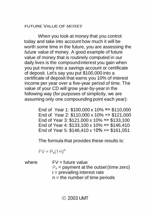
When you look at money that you control today and take into account how much it will be worth some time in the future, you are assessing the fufure value of money. A good example of future value of money that is routinely computed in our daily lives is the compound interest you gain when you put money into a savings account or certificate of deposit. Let's say you put $100,000 into a certificate of deposit that earns you 10% of interest income per year over a five-year period of time. The value of your CD will grow year-by-year in the following way (for purposes of simplicity, we are assuming only one compounding point each year):

End of Year 1: $100,000 x 10% => $110,000 End of Year 2: $110,000 x 10% => $121,000 End of Year 3: $121,000 x 10% => $133,100 End of Year 4: $133,100 x 10% => $146,410 End of Year 5: $146,410 x 10% => $161,051

The formula that provides these results is:

where FV = future value Po = payment at the outset (time zero) i = prevailing interest rate n = the number of time periods

O 2003 UMT

Future value looks at a cash flow today and projects its value at some time in the future. You routinely carry out this type of computation when you put money into a savings account or CD. However, let's say you are concerned with the reverse process. A friend who has borrowed $16,105 from you informs you that she cannot repay you until five years from now. If the prevailing interest rate you face is 10% (i.e., you have the opportunity to put your money into a 10% CD), you can compute from the data offered above that $16,105 five years from now is equal to $1 0,000 today, because you can take the $10,000, invest it at lo%, and have $16,105 in your account five years from now. (Note that in finance, what we call the prevailing interest rate is given the name cost of capital.)

When you look at a future cash flow and assess it in terms of today's money, you are conducting a present value analysis. Note that it is the reverse process of future value analysis. In fact, the formula for conducting present value analysis is the same as the formula used in computing future value with its terms rearranged slightly. That is:

Present value = Po = FV/(l +i)"

Table 2 shows present value computations for cash outflows, inflows, and net flows associated with two hypothetical five year projects, Project A and

O 2003 UMT

Project B. It assumes a prevailing interest rate of 10% year-by-year.

The bottom line for Project A is:

Total present value, cash outflows = $422.24 Total present value, cash inflows = $955.42 Total present value, net flows = $533.18

and the bottom line for Project B is:

Total present value, cash outflows = $422.24 Total present value, cash inflows = $907.48 Total present value, net flows = $485.24

0 2003 UMT

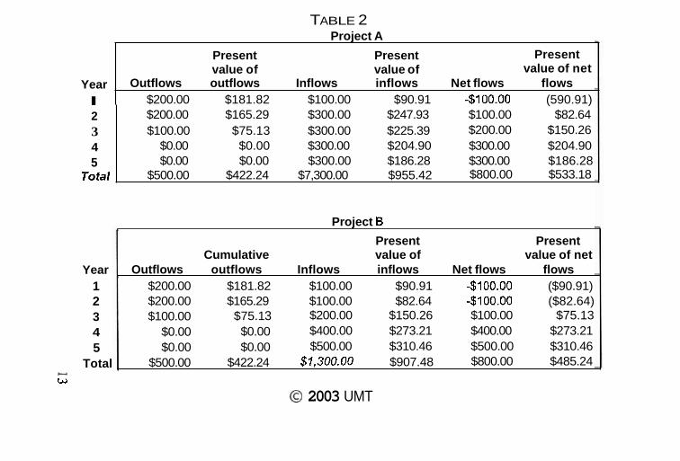
TABLE 2 Project A

Year 1 2 3 4 5

Total w W

Year I 2 3 4 5

Total

Project B

Present Present Cumulative value of value of net

Present Present Present value of value of value of net

Outflows outflows Inflows inflows Net flows flows $200.00 $181.82 $100.00 $90.91 -$100.00 (590.91) $200.00 $165.29 $300.00 $247.93 $100.00 $82.64 $100.00 $75.1 3 $300.00 $225.39 $200.00 $150.26

$0.00 $0.00 $300.00 $204.90 $300.00 $204.90 $0.00 $0.00 $300.00 $186.28 $300.00 $186.28

$500.00 $422.24 $7,300.00 $955.42 $800.00 $533.18

Outflows outflows Inflows inflows Net flows flows $200.00 $181.82 $100.00 $90.91 -$100.00 ($90.91) $200.00 $165.29 $100.00 $82.64 -$100.00 ($82.64) $100.00 $75.1 3 $200.00 $150.26 $100.00 $75.1 3

$0.00 $0.00 $400.00 $273.21 $400.00 $273.21 $0.00 $0.00 $500.00 $310.46 $500.00 $310.46

$500.00 $422.24 $7,300.00 $907.48 $800.00 $485.24

O 2003 UMT

The present value associated with net flows is an important concept in finance and is given the name netpresent value (NPV). A little thought shows that NPV is the present value of profit. When seen from this perspective, we conclude that once present values have been computed for the different cash flows, Project A is more attractive than Project B, because its true, discounted profit ($533.18) is greater than the discounted profit of Project B ($485.24). Note that before carrying out the present value analysis, Project A and Project B have the same level of profitability. In both cases, "raw" profit is $800, so it appears that A and B are equally attractive from the purview of profit. However, the present value analysis - which factors in the time value of money - makes it clear that A is actually more attractive than B.

When you look at present values for different values in a cash outflow or inflow stream, you are conducting what is called discounted cash flow (DCF) analysis.

NPV offers us a crude decision rule when trying to determine whether or not a potential project is worthy of support. The rule states that if NPV is positive, the project will be profitable, and therefore it is a possible candidate for support. If it is negative, the project will lose money and should not be supported.

How does one actually compute present value? If you work with Excel spreadsheets, you can use the NPV function to calculate present values. It

14 O 2003 UMT

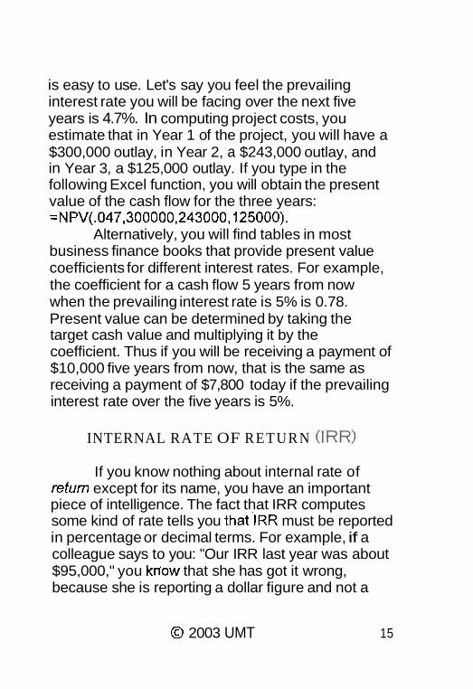
is easy to use. Let's say you feel the prevailing interest rate you will be facing over the next five years is 4.7%. In computing project costs, you estimate that in Year 1 of the project, you will have a $300,000 outlay, in Year 2, a $243,000 outlay, and in Year 3, a $125,000 outlay. If you type in the following Excel function, you will obtain the present value of the cash flow for the three years: =NPV(.047,300000,243000,?25000).

Alternatively, you will find tables in most business finance books that provide present value coefficients for different interest rates. For example, the coefficient for a cash flow 5 years from now when the prevailing interest rate is 5% is 0.78. Present value can be determined by taking the target cash value and multiplying it by the coefficient. Thus if you will be receiving a payment of $10,000 five years from now, that is the same as receiving a payment of $7,800 today if the prevailing interest rate over the five years is 5%.

INTERNAL RATE OF RETURN ( IRR)

If you know nothing about internal rate of refum except for its name, you have an important piece of intelligence. The fact that IRR computes some kind of rate tells you t h a t ' l ~ ~ must be reported in percentage or decimal terms. For example, if a colleague says to you: "Our IRR last year was about $95,000," you kn.ow that she has got it wrong, because she is reporting a dollar figure and not a

O 2003 UMT 15

percent. However, if this same colleague says to you: "Our IRR last year was 13.7%," at least she has got the units of analysis correct even if the number she reports is wrong.

IRR is a measure of return on investment. It is, in fact, one of several such measures, e.g., return on assets and return on equity. As such, IRR provides you with a sense of the "bang for the buck" of an investment. If one of your team members computes that the IRR associated with a specific project investment is 12% over a five year period of time, he is telling you that each dollar you invest in the project generates 12 cents of return each year. Is this good? To answer this question, you need to compare the anticipated project IRR figure with the rates of return you might encounter with other investment opportunities. For example, the 12% figure is higher than T-bill rates (e.g., 4.25%), CD rates (e.g., 5.0%), the interest rate on a checking account (e.g., 1 .I%), and the anticipated rate of return on Project C (e.g., 9.5%). The fact that it is so much higher than the alternatives makes this an attractive investment opportunity - at least from the financial perspective.

With IRR, we examine cash outflows and inflows for a fixed period of time (e.g., five years). With a typical investment, you spend money in the early time periods and make little or nothing in return. As time goes on, the balance shifts if the investment is paying off. By the later time periods, your cash outflows may have ceased and you are

16 @ 2003 UMT

making strong returns. In computing IRR, we are calculating your average performance, year-by-year (or month-by-month, or whatever other units of analysis you are using), for the fixed time period you are working with.

Table 3 illustrates IRR computations for Projects A and B. Note that both projects have the same NPV of $99.96. So from the perspective of "real" profit, the two projects are indistinguishable. However, because Project B has cash outflows occurring later than Project A, it has a higher IRR. Basically, the IRR figure of 23% is saying: "Select me. I am spending money later than Project A, when money is 'cheaper,' so I have a better rate of return. Project A is spending money early, when money is dear."

O 2003 UMT

Year

1

2

5 Total

Present value

Interest rate IRR

TABLE 3

Year

$200.00 $0.00 $200.00 1

$200.00 $0.00 $200.00 2

$100.00 $100.00 $0.00 3 $0.00 $200.00 $200.00 4 $0.00 $500.00 $500.00

Total Present

$422.24 $522.19 $99.96 value Interest

0.10 rate 19% IRR

O 2003 UMT

Table 4 offers insight into how IRR is actually computed. The table is comprised of three sub- tables, each of which has identical dollar values in the main body of the table. The only difference among the tables is that the present values are different, reflecting different interest rates. The first sub-table shows that NPV is $99.96 when the interest rate is 10%. The second shows that NPV drops to $37.80 when NPV is increased to 15%. The third shows that NPV becomes -8.17 when the interest rate is raised to 20%, reflecting a situation where the project is actually losing money. Somewhere between the 15% and 20% interest rate, the project goes from a money-making to a money-losing scenario. The actual breakeven point occurs when the interest rate is 19%. At this point, NPV is zero. The 19% figure is the IRR.

If a project's anticipated IRR is lower than the prevailing interest rate, it doesn't make sense to invest in it. You would be better off putting your money into some other investment vehicle where the returns are higher. This is what has occurred in Table 4 in the scenario where the prevailing interest rate is 2Q%, yet IRR is 19%.

0 2003 UMT

Table 4

lnterest rate = 15% Net

Outflows lnflows flows

lnterest rate = 10% lnterest rate = 20% Net

Oufflows lnflows flows

$200.00 $0.00 $200.00

$200.00 $0.00 $200.00 $100.00 $100.00 $0.00

$0.00 $200.00 $200.00 $0.00 $500.00 $500.00

$500.00 $800.00 $300.00

Year

1

2 3 4 5

Total

@ 2003 UMT

Net Oufflows Inflows flows

$200.00 $0.00 $200.00

$200.00 $0.00 $200.00 $100.00 $100.00 $0.00

$0.00 $200.00 $200.00 $0.00 $500.00 $500.00

$500.00 $800.00 $300.00

Present value $422.24 $522.19 $99.96

Interest rate 0.10 IRR 19%

On the other hand, if a project's IRR is higher than the prevailing interest rate, then it may be smart to invest in it. For example, in Table 4, when the prevailing interest rate is either 10% or 15%, and IRR is 19%, you will encounter greater gains supporting the project than investing your money at the prevailing interest rate.

When the prevailing interest rate and IRR are identical, neither one offers an advantage.

One final word before leaving IRR. When using IRR to help guide you in your project prioritization decisions, you should be aware of an important assumption of the IRR model. IRR computations assume that you are continually employing the money going into the project investment. That is, the money is generating returns around the clock, seven days a week. This is a somewhat frail assumption, since clearly there are times when the investment money is sitting in a safe or a low interest bank account, waiting to be allocated to the project. If the investment money earmarked for project use is poorly managed in a cash management sense, then the IRR computations significantly overstate the potentia! return on your investment. On the other hand, if the great bulk of the investment money is being used productively most of the time, this assumption should not be too harmful.

O 2003 UMT

Benefit-cost analysis has a long and distinguished history in project management. Its basic rationale is simple, although implementing an effective benefit-cost analysis can be tricky. At its roots, benefit-cost analysis is concerned with weighing the benefits of a decision against the costs. This sentiment is captured in the following statements:

"It's going to take us four hours, round trip, to get to Martha's party. Her party is likely to last two hours and we don't know any of the other invitees. Is it really worth trekking to Martha's place?" "In comparing Database A against Database B, our analysts have found that Database B saves us more money in operating expenses per dollar invested in the system, than Database A." "That imported Scottish salmon looks great, but it costs twice as much as our domestic salmon. I wonder if it is worth the extra expense?"

In this section, we look at one approach to conducting benefit-cost analysis: the benefit-cost ratio.

O 2003 UMT

COMPUTNG BENEFITLCOST RATIOS

The benefit-cost ratio is nothing more than a measure of benefit divided by a measure of cost. In theory, the measure of benefit can be anything: financial profit, cost savings, happiness, error reduction, throughput time, and so on. In practice, the measure of benefit is revenue - or in non- revenue generating situations, cost savings. We restrict our discussion here to treating benefits as revenue or cost savings.

The measure of cost is usually a conventional measure of money expended to carry out a project.

If benefits are assessed as revenue and costs as expenditures, the resulting ratio is easy to interpret. Consider the following three scenarios:

Benefit-cost ratio (B/C) > 1.0. In this case, revenue is greater than expenditures. That means that the investment is profitable. Example: B/C = $120,000/$50,000 = 2.4 Interpretation: For each dollar you are spending on this project, you are gaining $2.40 in revenue. Benefit-cost ratio (B/C) = 0.0. In this case, revenue and expenditures offset each other. You are not making net revenue, but neither are you losing money.

O 2003 UMT

Consequently, you are facing a breakeven situation. Example: B/C = $50,000/50,000 = 1.0 Interpretation: For each dollar you are spending on this project, you are making $1.00 in revenue. Thus you are breaking even.

+ Benefit-cost ratio (BE) < 1.0. In this case, expenditures outstrip revenue. You are losing money. Example: BIC = $40,000/$50,000 = 0.8 Interpretation: For each dollar you are spending on this project, you are only gaining 80 cents of revenue. Thus you are losing money.

EXAMPLE: COMPARING THE BENEFIT-COST PERFORMANCE OF TWO PROJECTS

Table 5 shows projected cash flow data for two projects, Project A and Project 8. It presents the data in both "raw" numbers and discounted numbers. The benefit-cost ratios for the two projects are:

Project A: BIC = $1,300/$500 = 2.6 Project 6: BIC = $1,400/$500 = 2.8

24 O 2003 UMT

Project B has the higher benefit-cost ratio. It is generating more "bang for the buck" than Project A.

Year

1 2 3 4 5

Total

Year 1

2 3 4 5

Total

Present value of

Outflows outflows

$300.00 $272.73 $200.00 $165.29

$0.00 $0.00 $0.00 $0.00 $0.00 $0.00

$500.00 $438.02

Project A Present

value of

Inflows inflows

$100.00 $90.91 $300.00 $247.93 $300.00 $225.39 $300.00 $204.90 $300.00 $186.28

$1,300.00 $955.42

Present

Net va20f 1 flows flows

$200.00 ($181.82) / $100.00 $82.64 $300.00 $225.39 $300.00 $204.90 $300.00 $186.28 $800.00 $51 7.40

Project B Present Present

value value of Cumulative of Net net

O U ~ ~ ~ O W S outflows Inflows inflows flows flows $100.00 $90.91 $100.00 $90.91 $0.00 $0.00

I

$200.00 $165.29 $100.00 $82.64 $100.00 ($82.64) ! $200.00 $150.26 $200.00 $150.26 $0.00 $0.00 1

$0.00 $0.00 $400.00 $273.21 $400.00 $273.21 ' $0.00 $0.00 $600.00 $372.55 $600.00 $372.55 i

$500.00 I $406.46 $1,400.00 $969.57 $900.00 $563.11

Let's now carry out benefit-cost analysis using the present value of cash inflows and outflows.

O 2003 UMT

Using discounted cash flow data for the two projects, we have:

Project A: Discounted B/C = $955.42/$438.02 = 2.18 Project B: Discounted B/C = $969.57/$406.46 = 2.39

By using discounted cash flow data, we see that Project B continues to outperform Project A. When you employ benefit-cost ratio analysis using discounted cash inflow and outflow data, you are computing what in finance is called the profitability index.

BENEF/T-COST ANAL YS/S WITH NON-REVENUE GENERATING PROJECTS

Many projects that are carried out are not revenue generating. This is true of infrastructure projects that are geared toward improving an organization's operations. For example, a typical information technology (IT) project is not revenue generating. When an organization upgrades its database management system, or adopts a customer relationship management (CRM) system, or enhances its network system, its chief goal is to enhance operations, not to increase sales. This can improve revenue performance indirectly, as the organization reduces operating costs. But it is not directly tied to generating revenue.

Government projects also do not generate revenue. Government's role is to provide services to

@ 2003 UMT

society to enable it to function effectively, not to make a profit.

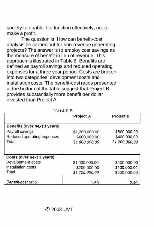
The question is: How can benefit-cost analysis be carried out for non-revenue generating projects? The answer is to employ cost savings as the measure of benefit in lieu of revenue. This approach is illustrated in Table 6. Benefits are defined as payroll savings and reduced operating expenses for a three year period. Costs are broken into two categories: development costs and installation costs. The benefit-cost ratios presented at the bottom of the table suggest that Project B provides substantially more benefit per dollar invested than Project A.

TABLE 6 Project A Project B

Benefits (over next 3 years) Payroll savings Reduced operating expenses Total

$1,200,000.00 $800,000.00 $600,000.00 $400,000.00

$1,800,000.00 $1,200,000.00

Costs (over next 3 years) Development costs Installation costs Total

@ 2003 UMT

$1,000,000.00 $400,000.00 $200,000.00 $100,000.00

$1,200,000.00 $500,000.00

~enefit-cost ratio 1.50 2.40

There are a number of pitfalls associated with benefit-cost analyses that are important to know. Three will be discussed here.

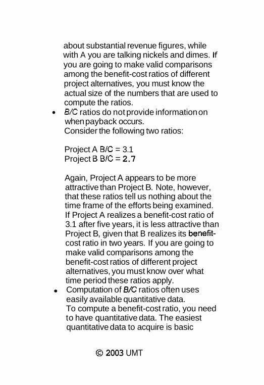
B/C ratios do not provide information on the size of the numbers being reviewed. Consider the following two ratios: Project A BIC = 3.1 Project B BIC = 2.7

The fact that Project A's benefit-cost ratio is notably higher than Project B's might suggest that A is the better project. Before jumping to this conclusion, it is a good idea to determine what numbers go into computing these ratios. In the case of Projects A and B, they are:

Project A BIC = 3,10011000 = 3.1 Project B BIC = 2,700,000/1,000,000 = 2.7

Note that when you divide one number by another, you lose a sense of the size of the numbers. There are in fact an infinite number of ways to generate a ratio of 3.1 (e.g., 31/10, 310/100, 3,10011,000, etc.). A little reflection suggests that for most organizations, Project B is more attractive than A, because with B you are talking

O 2003 UMT

about substantial revenue figures, while with A you are talking nickels and dimes. If you are going to make valid comparisons among the benefit-cost ratios of different project alternatives, you must know the actual size of the numbers that are used to compute the ratios. B/C ratios do not provide information on when payback occurs. Consider the following two ratios:

Project A B/C = 3.1 Project 6 BIC = 2.7

Again, Project A appears to be more attractive than Project B. Note, however, that these ratios tell us nothing about the time frame of the efforts being examined. If Project A realizes a benefit-cost ratio of 3.1 after five years, it is less attractive than Project B, given that B realizes its benefit- cost ratio in two years. If you are going to make valid comparisons among the benefit-cost ratios of different project alternatives, you must know over what time period these ratios apply. Computation of B/C ratios often uses easily available quantitative data. To compute a benefit-cost ratio, you need to have quantitative data. The easiest quantitative data to acquire is basic

O 2003 UMT

business data derived from estimated budgets and, possibly, marketing data on anticipated revenues. Hard-to-measure factors are often ignored when computing the ratios. For example, the chief benefit of a project may be what is called a second-order benefit - e.g., this project, while not profitable in itself, will provide the groundwork for major revenue streams generated on future projects. Has anyone made an effort to compute these second- order benefits? Another benefit might be improved public perceptions of the company's activities. Has anyone tried to figure out how to quantify an intangible factor such as the public's perception of a company's efforts?

None of these pitfalls is fatal. The point is that in doing benefit-cost ratio analyses, analysts should be aware of their existence and should strive to deal with them so that the analyses are valid.

INTEGRATING THE FlNANClAL TOOLS

Each of the financial tools examined in this chapter has its special value as well as its limitations. No one tool is "best." In fact, effective utilization of these tools to help prioritize projects requires that they be employed concurrently. For example, when reviewing a number of potential

30 0 2003 UMT

projects financially, you should see whether the financial prioritization tools reinforce each other in helping to choose a winner. If one project stands out because it has the highest NPV, IRR, and BIC ratio, and has a short payback period to boot, then this project is clearly worthy. On the other hand, if one project scores well on NPV, another on IRR, another on the BIC ratio, and still another on payback period, then you need to decide: Which of these financial measures is most important to me in making my decision?

Payback period's primary strength is that it enables you to determine when you are finally making more money than you spent. The earlier you can recoup your investment dollars on a project, the better.

NPV's principal strength is that it tells you how profitable a project is in terms of today's dollars. In general, projects with high NPV figures are preferable over those with medium or low NPV figures.

IRR's key strength is that it measures the return on investment for different projects, enabling you to compare each project's financial performance against other investment opportunities (e.g., CDs, treasury bills, other projects).

The BIC ratio's primary strength is that it offers you a straightforward measure of "bang for the buck." It answers the question: for each dollar 1 spend on a project, how much return can I anticipate achieving?

@ 2003 UMT 3 1

O 2003 UMT

A leading source of project failure is poor cost estimation. While bad estimates have created problems throughout the history of projects, their prevalence today is a major cause for concern. When you promise to do a $1,000,000 job for $600,000, you have hardwired cost overruns, schedule slippages and inadequate specification performance into your project before any work has begun. The link between bad cost estimates and cost overruns is obvious, while the triggering of schedule slippage and poor performance on specifications is a little more subtle. Schedule slippage can arise as a project begins to run out of money (which is what happens to projects that underestimate costs). As the money becomes scarce, work may slow down or stop entirely. Milestones are missed and the project falls hopelessly behind schedule. In addition, as the money disappears, there may be a temptation to cut corners, leading to unsatisfactory performance in respect to project specifications.

There are a number of explanations for the occurrence of bad cost estimates. They include:

O 2003 UMT

Sales people promise customers low- priced projects in order to make a sale and generate commissions Technical people tend to understate the technical difficulties of conducting a project The people making the estimates have no knowledge of proper estimating procedures and make serious errors when putting together cost estimates The estimates often make unrealistic assumptions about how efficient individuals, teams, and organizations are in carrying out projects - e.g., they assume project workers will be working full eight hour days, although research suggests that the very best project workers are lucky to be able to engage in five hours of productive work in a typical day The estimates are driven by political factors -this is reflected in such phenomena as support for the pet projects of powerful people, and the compulsion to "do whatever it takes to bring on new business"

Given the strong negative consequences of poor estimation, it is important that project professionals develop good estimation skills. In this chapter, we examine a number of significant

3 4 O 2003 UMT

perspectives and tools that lead to better estimation on projects.

HOW COST ESTIMATES ARE USED

Cost estimates serve a number of functions, including:

They provide managers with information on whether or not specific project alternatives are attractive and should be pursued They serve as the basis of bids They establish customer expectations on what it will cost to do a job They provided the foundation for developing project budgets

DIFFERENT LEVELS OF COST ESTIMATION

Cost estimates are dynamic. At different stages of a project, they take on different forms and purposes. For example, at the pre-project stage, there is insufficient information to develop a detailed and accurate cost estimate. As the project is launched, more information is available, so the estimates become more detailed. Once the project is fully established and basic plans have been developed, the estimates are even further refined. It is important to recognize that the estimating process

63 2003 UMT

continues right to the end of the project. For example, a month before the project's end, a cost estimate may be made to determine the cost of holding a project completion party!

Over the years, a general consensus has emerged in project management that cost estimates can be productively categorized into three levels: conceptual estimates, preliminary estimates, and definitive estimates. These three levels were first identified in the construction industry, but today they are employed across all industries.

For most projects, at the pre-project stage of the project life cycle, little thought has been given to the details of what it will take to execute a project. In fact, a decision has not yet been made as to whether the organization should support the project. The function of a cost estimate at this point is to provide managers with the information they need to make a golno-go decision.

Obviously, a problem with making estimates at this time is the lack of adequate information on just about all aspects of the project, including its duration, specifications, and tasks. Yet it is important that a solid cost estimate be developed so that managers will have at least a rough sense of the resources that need to be employed to execute the project.

@ 2003 UMT

When an estimate is made at this time, it is called a conceptual estimate (or in some circles, it is referred to as an order of magnitude estimate). No one seriously expects the estimate to be accurate. Also, no one has the time, resources or inclination at this point to carry out a massive effort to define the project so that accurate estimates can be made. What is needed is an estimate that offers a good sense of the rough magnitude of project costs.

The specific approach to making conceptual estimates is called top-down estimating. With this type of estimating, you take a look at the cost of similar projects, make a number of logical assumptions, and develop a quick estimate of project costs. This information becomes part of the body of data needed to decide whether or not to go ahead with the project. More will be said on top- down estimates later in this chapter.

PRELIMINARY ESTIMATES

Preliminary estimates are developed once a decision has been made to pursue a project. For example, in pricing a project to be included in a bid, you need more detailed and more accurate figures than you can derive from a conceptual estimate. So resources are released to create this estimate. Even now, however, the dearth of adequate information constrains you in making your estimate. While the preliminary estimate is more accurate than the conceptual estimate, it is still rather crude.

O 2003 UMT

Preliminary estimates may use either a refined top-down estimating procedure or a crude bottom-up procedure. With bottom-up estimating, you specify the tasks that will be carried out on a project, then cost each task, then tally up the cost estimates of all the tasks. More will be said about bottom-up estimates later in this chapter.

DEFlN/T/VE EST/MA TES

Definitive estimates are the most accurate estimates you can make. They usually are not fully developed until the project is underway. They are created as part of the funded project planning effort. At this time, a fairly detailed work breakdown structure (WBS) and project schedule have emerged. The work is now fairly well defined. The estimate invariably arises as the consequence of a bottom-up estimating effort.

An important function of definitive estimates is to provide the basis of developing a detailed project budget.

O 2003 UMT

BASE COST CATEGORIES

When making cost estimates or constructing a budget, you need to be aware of different categories of costs.

DIRECT VS. INDIRECT COSTS

Direct costs are costs that reflect work, equipment and materials employed directly in a work effort. For example, the salaries of engineers employed on a project, a router rented to customize molding, and the price of lumber used to frame a house are each examples of direct costs.

Indirect costs are costs incurred to support the directly productive work effort. Overhead (e.g., the price of electricity, office rent, the cost of maintaining a secretarial pool) and fringe benefits (e.g., life insurance, pension plans, profit sharing schemes) are examples of indirect costs.

An objective of cost-conscious organizations is to reduce indirect costs to the extent possible. Elegant headquarters, the use of a corporate jet, and munificent pension plans all contribute to the swelling of indirect costs. They may make the work environment attractive to senior executives, but in the final analysis they add to the cost of doing business and reduce profit margins.

0 2003 UMT

VARIABLE VS. FIXED COSTS

Variable costs are costs directly tied to carrying out a work effort. When building a house, the cost of lumber is a variable cost. The more lumber that is used, the higher the overall cost of lumber. If no lumber is used, then the cost of lumber is zero.

Fixed costs are costs that will be incurred whether or not an asset is actually employed. For example, if you are paying off the mortgage for your office building, a defined monthly mortgage payment is due to the bank whether or not the company has actually transacted business during the month. Typical examples of fixed cost items include real estate and installed machinery.

An interesting question is whether labor costs are variable costs or fixed costs. Superficially, they would appear to be variable costs -the more you employ a worker on the job, the more you can charge for that worker's effort. However, in recent years, labor costs have increasingly been viewed by business people as fixed costs because you cannot readily hire people when demand for services is high and fire them when business is slow. During slow times, workers are often retained on the payroll even if they are not fully employed - at least for the short run. In this sense, then, labor is viewed as a fixed cost item.

O 2003 UMT

Top-down estimates tend to be "quick and dirty." They are carried out simply to develop a rough sense of what level of resources a project will consume. They can be quite accurate if an organization has carried out many projects of a similar nature and has a rich database reflecting previous cost experiences.

The best-known top-down cost estimating technique is called parametric cost estimating. In mathematics, the world parameter means "constant." (In an algebraic equation, you have variables and constants, and the technical term for constant is parameter.) With parametric cost estimating, you identify pertinent cost constants and use them to help you estimate project costs.

Construction estimators make heavy use of parametric cost estimating. For example, in estimating how much money it will cost to build a warehouse, they take the number of square feet of floor space (a variable) and multiply it by a cost-per- square-foot figure (a parameter) they have that reflects the cost of building warehouses. If the cost- per-square-foot figure is on target, the resulting cost estimate can be quiteaccurate.

Consider another simple example: Let's say you are driving by a gas station and see the price of gas posted on a large sign next to the gas pumps. It says: "Regular Gas - $2.00 per gallon." You note

O 2003 UMT

costs for these items encountered on similar projects.

An important measure reported in Table 7 is found at the bottom of the table. It is called the loading factor and helps you to account for fringe benefits and overhead costs when you report your workers' loaded (also called fully burdened) wage rates. In this case, the 2.21 value tells you that for each dollar of wages a worker is paid, the cost to the company of employing that worker is $2.21. Consequently, if you estimate that your workers will be paid $10,000 to carry out a task, you can figure that the total cost to your organization will be $22,100. Continuing with this logic, you see that your $40 per hour engineers really cost you $88.1 0 per hour, and you should bill them out at a rate that covers this cost and also factors in profit.

O 2003 UMT

TABLE 7 Parametric Cost Estimating

Labor Engineers (400 person hours of work @ $401hr ) $16,000.00 Technical support $1.000 person hours of work @ $25/hr $25,000.00 Subtotal: Labor $41,000.00 $41,000.00

Fringe benefits Fringe benefits (30% of labor costs) $12,300.00 Subtotal: Fringe benefits $12,300.00 $53,300.00

Overhead Overhead (70% of labor costs plus fringe benefits) $37,310.00 Subtotal: Overhead $37,310.00 $90,610.00

Other costs Report production Travel Subtotal: Other costs

Total $102,610.00

Loading factor 2.21

The good news about bottom-up cost estimates is that they are generally more accurate

44 O 2003 UMT

than top-down estimates, because they have been developed with substantial care and have explicitly taken into account all the cost elements of a project. The bad news is that it takes an enormous amount of time and resources to create a good bottom-up estimate.

Bottom-up estimates are derived from work breakdown structures (WBSs). WBSs come in three formats: product-oriented, task-oriented, and mixed format. These are illustrated in Tables 8, 9, and 10 respectively. The definitive document describing the structure and function of WBSs is titled Practice Standard for Work Breakdown Structures and is published by the Project Management Institute. (It can be ordered from the PMI website at www.pmi.orq.).

Table 8 portrays the product oriented WBS. This is the approach to WBS construction followed by the US Department of Defense. It focuses on the deliverable and its constituent parts. Notice the role of the numbering system that identifies each WBS element. This numbering system is called the code of accounts. It identifies where in the overall WBS a given WBS element sits. Note also that the most detailed elements of the WBS are called work packages. These work packages are important in bottom-up cost estimating, because they capture cost data for the project. For example, WBS element 1 .I .I Survey has $1,000 worth of activity and materials associated with it. WBS element 1.1.2 Digging has $3,000 of activity and materials

O 2003 UMT

associated with it. By adding the cost data for 1 .I .I and 1.1.2, we find that 1 .I .0 Excavation has $4,000 dollars of activity and materials associated with it. This process of rolling up data from the bottom of the WBS to the top is how bottom-up costs estimates are made.

Work packages

Table 8 WBS

element 1.0.0

1.1.0 1.1.1 1.1.2

Product-oriented House 4 WBS

Excavation Survey ($1,000) Digging ($3,000) Foundation Preparatory work ($2,000) Pouring ($4,000) Framework Site preparation ($2,000) Construction ($1 5,000) Plumbing Site preparation ($1,000) lnstallation ($5,000) Wiring Site preparation ($1,000) Installation ($4,000) Roofing Site preparation ($2,000) Installation ($7,000) Interior work Drywall ($10,000) Painting ($4,000)

@ 2003 UMT

TABLE 9 I WBS

element 1 .o.o

1.1.0 1.1.1 1.1.2

1.2.0 1.2.1 1.2.2

1.3.0 1.3.1 1.3.2

1.4.0 1.4.1 1.4.2

1.5.0 1.5.1 1.5.2

1.6.0 1.6.1 1.6.2

1.7.0 1.7.1 1.7.2

Task-oriented WBS Build the house Excavate the land Conduct survey Excavate the marked places Work on the foundation Prepare for pouring the foundation Pour the foundation Construct the framework Prepare the site Put up the framework Install the plumbing Prepare the site for installation Install the pipes Install the wiring Prepare the site for wiring Hang and connect the wiring Put the roof on the house Prepare for roofing work Carry out roofing work Work on the house's interior Hang and tape the drywall Paint the walls

Table 9 pictures a task-oriented WBS. Most of the project management scheduling software packages -such as Microsoft Project - employ task- oriented WBSs. As with the product-oriented WBS, the task-oriented WBS uses a code of accounts to identify individual WBS elements. Also, although

O 2003 UMT 47

cost data are not offered in Table 9, task-oriented WBSs support the collection of cost data at the work package level, enabling bottom-up cost estimates to be carried out by rolling up the data from the bottom of the WBS to the top.

WBS element 1 .o.o

1 .I .o 1.1.1 1.1.2

1.2.0 1.2.1 1.2.2

1.3.0 1.3.1 1.3.2

1.4.0 1.4.1 1.4.2

1.5.0 1.5.1 1.5.2

1.6.0 1.6.1 1.6.2

I .7.0 1.7.1 1.7.2

Mixed WBS House Excavation Conduct survey Excavate the marked places Foundation Prepare for pouring the foundation Pour the foundation Framework Prepare the site Put up the framework Plumbing Prepare the site for installation Install the pipes Wiring Prepare the site for wiring Hang and connect the wiring Roofing Prepare for roofing work Carry out roofing work Interior Hang and tape the drywall Paint the walls

O 2003 UMT

Table 10 is a mixed WBS. High level WBS elements such as 1 . I 0 Excavation and 1.2.0 Foundation are product-oriented. WBS elements below them, such as 1 .I .I Conduct survey and 1 .I .2 Excavate the marked places, are tasks. It appears that this approach to WBS construction is becoming the most popular. As with the product-oriented and task-oriented WBS, the mixed WBS can be employed to carry out bottom-up cost estimates.

COST ESTIMATING WITH PERT BETA

In the late 1950s, while working on the Polaris Missile Program, the US Navy developed what became the best-known project scheduling technique: the Program Evaluation and Review Technique (PERT). This technique borrowed flow charting concepts from the newly emerged discipline of systems engineering. It pictured graphically how project tasks are linked together by means of dependency relationships. While the Navy engineers had no problem mapping their projects with the PERT format, they were puzzled about how to make estimates of task durations for the pictured tasks. So they went to statisticians for guidance on this matter. The statisticians showed them a clever way of estimating task durations, provided you have a sense of the shortest time, most typical time, and slowest time it might take to do a job. The estimated durations can be computed using the following, simple formula:

@ 2003 UMT 49

Expected duration = (Best case + 4*Most typical case + Worst case)l6

This formula is called the PERT Beta formula, because it is assuming that the task durations are distributed roughly in the shape of a Beta distribution.

Let's say we are using this formula to calculate the expected duration for installing a piece of equipment. Historical data we have suggests that the fastest this equipment has been installed is three hours. The slowest installation time on record is seven hours. Most typically, the installation takes four hours. Plugging these values into the PERT Beta formula, we have:

Duration = (3 hours + 4*4 hours + 7 hours)/6 = (26 hours)/6 = 4.33 hours

Thus the best estimate of how long it will take to install the equipment is 4.33 hours.

This same formula can be used in cost estimating and estimating manpower requirements as well. Let's say that cheapest cost we have experienced in installing a piece of equipment is $3,000. When things go badly, it can cost up to $7,000. Typically, it costs $4,000. Plugging these values into the PERT Beta formula, we have:

Costs = ($3,000 + 4*$4,000 + $7,000)/6 = $26,00016 = $4,333

O 2003 UMT

Thus the best estimate of installation costs is $4,333.

Increasingly, customers are asking project teams to devise lifecycle cost estimates. Lifecycle cost estimates have two defining characteristics. First, they look at cost allocations over multiple time periods (e.g., money spent week-by-week, month- by-month, or year-by-year). This stands in contrast to the traditional cost estimate, which typically reports a single cost figure for the whole time span being considered. By looking at cost allocations over multiple time periods, life-cycle cost estimates provide a dynamic view of project activity. Like a cash flow statement, they enable project team members to identify when cash outflows will be large and when they will be small. This information is important if a project manager wants to make sure that sufficient funds are being released at different points in time to cover expenses over the life of the project.

Second, lifecycle cost estimates not only look at estimated project expenditures, but at expenditures incurred after the project is complete - these are called operations and maintenance costs. Thus a lifecycle cost estimate provides you with a complete view of project-related costs. If you only look at project costs, you typically see aminority of

0 2003 UMT

the expenditures associated with producing and operating a deliverable. But when you also examine operations and maintenance costs, you have a good sense of the total costs you will be facing.

Table 11 shows a lifecycle cost estimate for a 15-month undertaking. The project is carried out from Month 1 through Month 6. Then in Month 7 , project expenditures cease, indicating that the project phase is over. In Month 7, operations and maintenance expenses are incurred for the first time, indicating that the project's deliverable is now being employed. The last column summarizes the cost data over the fifteen month period being reviewed. It illustrates a typical scenario, where more money is being spent to operate and maintain a solution ($300,000) than to create it ($220,000).

Because lifecycle cost estimates are developed on electronic spreadsheets, they are easy to manipulate. They can show raw data or inflation-adjusted figures. They can picture best case, worst case, and most typical scenarios. They can even be used as a what-if modeling tool, enabling analysts to see cost impacts associated with different assumptions.

Budgeting is the process of determining how money will be allocated over time to carry out project work. To create a budget, you must have a good sense of what tasks are scheduled to be

63 2003 UMT

implemented, how many human and material resources will be employed, the cost of these resources, and when the money to do the job will be spent.

Budgets can be formulated with varying degrees of specificity. They can be high level, indicating the total dollar amount of resources that need to be allocated month-by-month, or they can be highly detailed, specifying funds earmarked for particular purposes, such as purchasing nuts and bolts, painting a sign, or testing a software application.

O 2003 UMT

Project Costs Design Build Test Subtotal

Operations & maintenance Recurring maintenance Preventive maintenance Operating costs Subtotal Grand total

TABLE 1 1 Lifecycle Cost Estimate (Figures are in

$10,000 units)

Total Month LCC

1 2 3 4 5 6 7 8 9 1 0 11 12 13 14 15

O 2003 UMT

CODE OFACCOUNTS

When budgets are presented at a detailed level, funding categories are often defined according to a code of accounts. A code of accounts is simply a way of organizing cost categories intelligently. A segment of a code of accounts is illustrated in Table 12.

PICTURING BUDGET DA TA

Budget data can be presented both in a tabular format or graphically. The graphical format is attractive if a manager wants to report budget activity to other people in an understandable, attractive format. Table 13 shows total budget data for a project, categorized according to cost category. The same data contained in Table 13 is portrayed graphically in Figure 1.

O 2003 UMT

TABLE 1 2 Code of Accounts (Partial)

13.0.0 Travel 13.1.0 Transportation 13.1.1 Airplane 13.1.2 Rail 13.1.3 Car 13.1.4 Other

Local 13.2.0 transportation 13.2.1 Taxi 13.2.2 Limo 13.2.3 Other 14.0.0 Lodging 14.1.0 Hotel 14.2.0 Other 15.0.0 Meals 15.1.0 Breakfast 15.2.0 Lunch 15.3.0 Dinner

ABC Project Budget, by Cost Category

Professionals $120,000 Support staff $70,000 Fringe benefits $57,000 Overhead $172,900 TOTAL $419,900

O 2003 UMT

ABC Project Budget, by Cost Category

-.

Professionals rn Support staff Fringe benefits Owrhead

Table 14 shows budget data for a project located over an eight month period. It presents the hta both on an actual month-by-month expenditure ~sis, as well as on a cumulative basis. The ~mulative budget data is captured in Figure 2. 'hen cumulative cost data are presented, they ten take on an S shape - consequently, the ~mulative budget curve is also called the S-curve.

0 2003 UMT

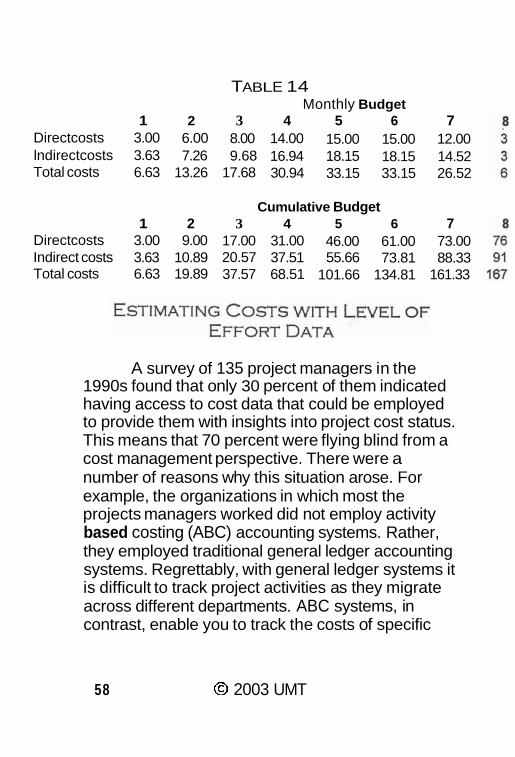
TABLE 14 Monthly Budget

1 2 3 4 5 6 7 Directcosts 3.00 6.00 8.00 14.00 15.00 15.00 12.00 lndirectcosts 3.63 7.26 9.68 16.94 18.15 18.15 14.52 Total costs 6.63 13.26 17.68 30.94 33.15 33.15 26.52

Cumulative Budget 1 2 3 4 5 6 7

Directcosts 3.00 9.00 17.00 31.00 46.00 61.00 73.00 Indirect costs 3.63 10.89 20.57 37.51 55.66 73.81 88.33 Total costs 6.63 19.89 37.57 68.51 101.66 134.81 161.33

A survey of 135 project managers in the 1990s found that only 30 percent of them indicated having access to cost data that could be employed to provide them with insights into project cost status. This means that 70 percent were flying blind from a cost management perspective. There were a number of reasons why this situation arose. For example, the organizations in which most the projects managers worked did not employ activity based costing (ABC) accounting systems. Rather, they employed traditional general ledger accounting systems. Regrettably, with general ledger systems it is difficult to track project activities as they migrate across different departments. ABC systems, in contrast, enable you to track the costs of specific

58 O 2003 UMT

tivities regardless of what department they occur The point is that without ABC accounting stems, the cost data you have may not map ?aningfully to the work that is being done.

Cumulative Budget over 8 Months

1 200.00 - 0

150.00 r

2s 100.00 - f = 50.00 - --

2 0.00 - 1

1 2 3 4 5 6 7 8

Month

-+ Direct costs - -) - Indirect costs +Total costs

Other standard problems included: cost data ?re being reported months after expenditures were :tually incurred; cost data were inaccurate owing to lor data capturing procedures; and cost data were lt being reported at all because they were viewed i secret.

The point is that it appears that a large ~mber of people working on projects do not have :cess to decent cost data. The good news is that

O 2003 UMT

we know how to estimate these data, provided we know three things: I ) the number of resources assigned to the job, 2) the amount of time they are (or will be) spending on their tasks, and 3) their average daily wage rates. The first two items enable us to compute something called level of effort. The third enables us to develop reasonably accurate estimates of cost, given that we know what the level of effort is.

Level of effort is a simple measure of work effort. If I have three ditch diggers digging ditches over a five day period of time, I can say that they will carry out fifteen person-days of effort. The fifteen person-days of effort is level of effort. Furthermore, if I know that these ditch diggers earn an average of $1 00 per day, I can estimate that they will earn a total of $1,500 (15 person-days of effort x $100 per day) to do the job. A little thought shows that level of effort is, in fact, budgetary currency. If you lack basic cost data on your project activities, you can back into a dollar estimate of the work effort by multiplying your level of effort computation by average per day wages.

In project management, level of effort estimates are commonly used to obtain a rough sense of project costs. For example, at the outset of the 2000s, Wall Street firms computed that the cost to them of employing a professional level information technology worker averages out to roughly $225,000 per year (including overhead and fringe benefit costs). Thus if they have a project that will require

@ 2003 UMT

use of two IT workers for three months (i.e., a total of a half a person-year of effort), they can reckon that the cost of using these workers will be about $1 12,500.

O 2003 UMT

O 2003 UMT

During project implementation, one of the key responsibilities of project management is to measure cost performance. This responsibility entails monitoring cost performance to detect and analyze variance from the budget. Cost control is achieved when management takes the necessary corrective action on detected variances to keep project expenditures within the bounds of the budget.

In this chapter, we examine the cost control tools that are commonly used on projects. Specifically, we look at variance analysis using the variance chart, S-curves and Earned Value Management (EVM).

Cost variance analysis is a simple method for measuring the extent to which actual project costs are in line with budgeted costs. Table 15 presents information on budgeted cost, actual cost, and cost variance for a 6-month project. Months 1 and 3 have positive cost variances, indicating that less money was spent in those months than planned. The other months - Months 2, 4, 5, and 6 - experienced cost overruns.

@ 2003 UMT 63

TABLE 15 Month

1 2 3 4 5 E Budget $40.000 $50,000 $45,000 $50,000 $55,000 $52 Actual cost $38,000 $53,000 $44,000 $54,000 $56,000 $58 Variance $2,000 -$3,000 $1,000 -$4,000 -51,000 -$4

The data in Table 15 are pictured graphically in Figure 3, which is called a variance chart. Note the zero variance line that runs across the chart. Markers that appear on or near this line reflect small variances or no variances. The further removed a marker is from this I~ne, the greater the cost variance that IS being portrayed. Markers above the line indicate cost underruns, while those below the line indicate cost overruns.

Figure 3

O 2003 UMT

Project Cost Variance over 6 Month Period

Month

The cost variance chart is good at picturing tterns in variances when they occur. This is seen =igure 4, which shows a project whose cost ?rruns are growing month-by-month. When lking at variances, the normal "pattern" you should counter is a random distribution of markers. ughly half should be above the zero variance line d half below. This random pattern tells you that J are basically on target in achieving your budget. wever, when a non-random pattern arises - as in lure 4 -this indicates that something unusual is opening. In these situations, it is important to mntify the cause of the pattern. If the pattern lects a serious problem, then you need to solve it.

0 2003 UMT

The important point here is that the variance chart serves a diagnostic function, enabling you to determine whether things are basically on course, or whether some potential problem exists.

Project Cost Variance over 6 Month Period

Month

C O S T CONTROL WITH S - C U R V E S

The S-curve is the most heavily used tool for monitoring cost variances. In Chapter 3, we saw that S-curves are constructed from cumulative budget data. When a budget S-curve is juxtaposed against an S-curve portraying actual costs, budget variances are highlighted. Figure 5 provides an example of S-

O 2003 UMT

,es used to identify budget variances. It reports : status as of Month 5. At this time, cumulative ~ a l costs are greater than cumulative budgeted :s, indicating that the project is encountering a : overrun. (Note that when the project first began, :perienced cost underruns.)

rEGRATED COST/~CHEDULE CONTROL

S-Curves for Budget and Actual Expenditures

$35,000 -

Although a review of an S-curve may show t you face a cost overrun on your project, this is necessarily bad. Similarly, if an S-curve shows t you are under budget, this is not necessarily ~ d . By themselves, budget variances only provide

$30,000 - e $25,000 - E $20,000 ; $15,000 -

$1 0,000 -- $5,000 -

O 2003 UMT

__.--- %%=* --

---- - - - - -- - _ .-2 - - - - -

__....--. - -

- -

$0 7 1 2 3 4 5 6

Dollars

+Budget - - .) . - Actual cost

partial information of a project's status. To know whether or not you are in trouble, you need to know how much work has been done, in addition to budget status. For example, while you may be facing a cost variance on the project, you may also find that you are dramatically ahead of schedule. The cost variance might simply reflect that earlier on the project you had an opportunity to finish more work than planned. On the one hand, you spent you money more quickly than planned - creating a cost overrun - but you are getting the job done more quickly than initially scheduled. By the same token, a cost overrun may simply reflect the fact that you are not doing much work. One way to "save" money is not to spend it!

The lesson here is that it is dangerous to look at cost variances in isolation from reviews of schedule status. Cost and schedule performance really must be carried out simultaneously. This principal of examining the two concurrently is called integrated cost/schedule control.

GRAPHICAL INTEGRATED COST/SCHEDUL E CONTROL

A good way to engage in integrated cost/schedule control is to work with two charts. The S-curve, as we have just seen, enables us to track project cost performance. A glance at it shows whether we are over budget, on budget, or under budget. A Gantt chart can be employed to reveal

G 8 O 2003 UMT

schedule performance. Gantt charts are simple bar charts that show when tasks are planned to be executed, and when they are actually executed. As with S-curves, they enable analysts to determine schedule status at a glance.

Figure 6 shows the S-curve and Gantt chart for a hypothetical project. While the S-curve indicates that there is a cost underrun, the Gantt chart shows schedule slippage. If you only consider cost performance, you might be deluded into thinking that the project is saving money. The Gantt chart makes clear that this is not the case, since it demonstrates that there is schedule slippage -work is not being carried out according to the schedule.

O 2003 UMT

Dollars

/NTEGRA TED COST/SCHEDULE CONTROL WITH EARNED VALUE MANAGEMENT (EVMI

It would be cumbersome to carry out integrated cost~schedule control exercises on large projects that have hundreds or thousands of tasks. Project analysts would soon find themselves overwhelmed trying to make sense out of scores of Gantt charts and S-curves.

In the late 1960s, the US Department of Defense implemented a new approach to performing integrated cosffschedule control analyses using cost accounting precepts. They called this approach the cost/schedule control system, and it was often referred to as CISCS. In the 1990s, as the methodology was adopted by the private sector on a large scale, a consensus emerged among government and business players to change its name in order to make it sound less bureaucratic. It is now called the earned value management (EVM) system.

At the heart of EVM is the attempt to measure work performance. The basic question that needs to be answered is: How much of the job have you actually done? Until this question is answered, you really cannot interpret your cost and schedule status meaningfully. For example, the data may show that you have a ten percent cost overrun this month. Is this good or bad? Who knows? The only way to determine your status is to have a good sense of the amount of work you have accomplished. A ten

0 2003 UMT 7 1

percent cost overrun is not bad if it turns out that during the month you got twenty percent more work done than planned! On the other hand, a ten percent cost overrun is quite troublesome if during the month you only did eighty percent of what you were supposed to do.

The trick is to figure out how to measure work performance. In EVM, work performance is captured in a measure called earned value. Earned value tells you what share of what you planned to do has actually been done. Because it is a cost accounting concept, it is measured in dollar terms. Thus if you were supposed to complete a $1,000 budgeted task by today, but you have only done half the work, earned value is $500.

Knowing earned value allows you to determine cost and schedule status for your work effort. For example, if you were supposed to do $1,000 worth of work by today, but have only done $500 worth of work, your schedule variance is 4500 -that is, you have done $500 less work than you were supposed to do. Furthermore, if you spent $700 to do $500 worth of work, you have a cost variance of -$200 -that is, you spent $200 more than you should have for the work you have achieved.

There are several different ways to compute earned value. Three dominate: tracking milestones,

72 O 2003 UMT

employing the 50-50 rule, and simple guessing. Each will be discussed in turn.

TRACKING MLESTONES

The most accurate way to compute earned value is by tracking carefully constructed milestones. This approach will be described by means of a simple example.

Master Publishers is a small printing company that specializes in publishing workbooks and instruction books for education and training organizations. They have a contract to print, bind, box, and ship 20,000 150-page workbooks in a six- week time frame for a government client. The government client is supplying them with the workbook content in machine readable form, so Master Publishers does not need to engage in any design or layout work.

Experience on previous projects shows that a given workbook is 20% complete once if has been printed, 70% complete once it has been put into a binder, 90% complete once it is boxed, and 100% complete affer it has been shipped.

Table 16 provides data on the status of the project at the end of Week 2. An analyst has counted the physical document items at different stages of the production process. This information is reported in the column titled "Number of items counted at work station. " The weighted average of the work done is computed by taking the number of

O 2003 UMT

items counted and multiplying this figure by the percent of thejob that is done. This information is reported in the column titled "Weighted average of work done. "As the table shows, the weighted average of work done translates into having done all the work on 7,200 workbooks. Thus 36% of the workbook production effort is complete (i.e., 7,200/20,000). Since the project is a third finished (i.e., the status report indicates sfatus at the end of Week 2 for a six-week project), it is basically on schedule. If in addition cost status data indicates that the project has consumed about a third of its budget, fhen we can conclude thaf the project is on budget.

0 2003 UMT

TABLE 16 Measuring Work Performance for Workbook Production Project

Milestone in Production Process Aaterial ready to be processed Aaterial is printed Aaterial is put into loose leaf binder Aaterial is boxed Aaterial is shipped Veighted average of completed workbooks 'ercent ofjob done

Percent of job that is done

0% 20% 70% 90%

100%

Number of items counted at work station

5000 8000 4000 2000 1000

Weighted average of work

done 0

1600 2800 1800 1000 7200 36%

TMPLOVNG THE 50-50 RULE

The principal drawback to using milestones to neasure work performance is that you need to have lata on how much work performed each milestone :aptures. On most projects, this information is not wailable.

The 50-50 Rule does not require historical lata to measure work performance. It takes a tatistical approach. When a task begins, it holds the iew: "Let's assume we have achieved half the value ~f the task." Thus for a $320 task, it assumes $160 lf work has been accomplished the moment the task legins. Only when the task is actually completed, {ill it close the books on it and assume that the full alue of the task has been achieved. Thus when the

O 2003 UMT

$320 is finally done -whether it be completed on time or one month late -we say: "We have now completed $320 worth of planned effort."

The rationale behind the 50-50 rule is readily explained with a numerical example. Table 17 shows budget and work performance data for a five task project. All of the tasks on the list are supposed to be completed for the reporting period. A glance at the table shows that Task E is not complete, so clearly not all the work that was supposed to be done has been accomplished.

To compute earned value with the 50-50 Rule, you say that half the work is done the moment a task begins, and then say that the remaining half has been achieved once the task is finished. The only task that is not completed in Table 17 is Task E. Since it has begun, half the value of the task is counted (i.e., $100). However, the full value cannot be reported until the task is actually done.

By adding up the numbers in the earned value column, you are able to calculate the "dollars worth of work" that has been achieved on the project. In our example, this figure is $830, and is the measure of earned value. If we were on schedule, we should have achieved $930 worth of work (i.e., the total figure in the budgeted cost column). We can deduce that we have done 89.2% of what we should have done at the time of this status report (i.e., $830/$930).

People who work in the information technology arena often prefer to employ another rule

76 @ 2003 UMT

-the 0-100 Rule, which is more conservative than the 50-50 Rule. They maintain that a task has no value until it is complete. In Table 17, earned value would be $730 if the 0-1 00 Rule were employed, because no value would be recorded for Task E. Consequently, the percentage of the job done would be 78.5% ($730/$930).

TABLE 17 Using the 50-50 Rule to Compute Earned Value

Has Budgeted task Has task Earned

cost begun? finished? value

Task A $160 4 4 $160

Task I3 $220 4 4 $220

Task C $1 90 d 4 $190

Task D $160 4 4 $160

Task E $200 4 $100 Total $930 Earned value $830 Percent of job done 89.2%

So which is better, the 50-50 Rule or 0-100 Rule? The answer is "both." When estimating work performance, it is a good idea to use both rules. The 0-1 00 Rule gives you a conservative sense of how much work has been achieved. You cannot get a lower value! The 50-50 Rule is sort of a rule of the mean. By employing it, you are saying: "It is likely that I have done $830 worth of work." If you use both rules, you can make a statement such as: "I am

O 2003 UMT 77

pretty confident that I am between 78.5% and 89.2% of where I should be."

SIMPLE GUESSWORK

If you have no recourse to estimating earned value systematically, then you may have to fall back on good guesswork. A problem with guesswork is that it usually overstates how much work has been achieved and can lead to what is called the ninety percent hang-up. Here is how the ninety percent hang-up works:

At the end of Month 6, George is asked: How much of the job is done? He responds: "Seventy-five percent." At the end of Month 7, George is asked again: How much of the job is done? This fime he responds: "Ninety percent. " At fhe end of Month 8, George is asked again: How much of the job is done? He answers: "Ninety percent." At the end of Month 9, George is asked: How much of the job is done? He answers: "Ninety percent. "

Clearly, George is not ninety percent done. If he were to compute earned value objectively, he may learn that he is only eighty percent done. But as projects are carried out, and the easy chores are accomplished, team members develop confidence that they are making rapid progress. However, as projects approach the end of their lives, they tend to get bogged down. The whole solution must be integrated. Tests show that it doesn't work quite the way it is supposed to, and the system must be

O 2003 UMT

tweaked to get it to function properly. Time must be set aside to prepare documentation. And so on. This phenomenon is so commonly encountered on projects that we even joke: "The last ten percent of a project takes fifty percent of the work."

ASSESSING C O S T A N D SCHEDULE PERFORMANCE

You now know enough about the principles of earned value to carry out an integrated cosffschedule control analysis. The information you need to conduct this analysis is contained in Table 18.

Schedule stafus. The table shows that you have done $830 worth of work, but you were supposed to have done $930 worth of work. Consequently, you have done less work than planned. Your schedule variance is -$TOO, and is computed with the formula:

SV= EV- PV

where SV is schedule variance, EV is earned value, and PV is planned value (i.e., budget).

The proportion of the targeted work that you have actually completed is computed with the schedule performance index (SPI). Its formula is:

SPI = EVIPV

O 2003 UMT

Note that this ratio provides information about what portion of the planned effort has actually been achieved. In our example, SPI is 0.89, indicating that this project has achieved 89% of what it was supposed to achieve.

Cost status. Table 18 shows that it cost $91 0 to do $830 worth of work. Consequently, you can deduce that you are facing a cost overrun. Your cost variance is 480, and is computed with the formula:

where AC is actual cost. A measure of the efficiency with which you

are spending your money is computed with the cost performance index (CPI). Its formula is:

CPI = EVIAC

In our example, CPI is 0.91. This tells us that for each dollar you are putting into the project, you are getting 91 cents of work accomplished. In other words, your project is consuming more resources than it is generating value!

Finally, we have enough information to estimate the final cost of the project. In the EVM system, the estimate of final costs is called estimate at complete (EAC). It is computed with the following formula:

EAC = Project budget1CPI

80 @ 2003 UMT

This formula reflects common sense logic. Let's say a given project has a CPI of only 0.5. That means that it is generating 50 cents of value for each dollar invested in it. If the project has a $10,000 budget, and it continues to get 50 cents on the dollar, common sense suggests it will cost $20,000 to do the job. The EAC formula computes this: $10,000/0.5 = $20,000.

In Table 18, we see that for your project, Tasks A through E are budgeted to cost a total of $930. The CPI suggests that to date, the project has been getting 89 cents of value on the dollar. If you continue to get 89 cents on the dollar, then the projects EAC will be:

EAC = $930/0,89 = $1,020.

This means that the final cost of the project will be larger than originally planned. Either you need to get additional funding to complete the project or you should reduce the scope of what you will be delivering.

O 2003 UMT

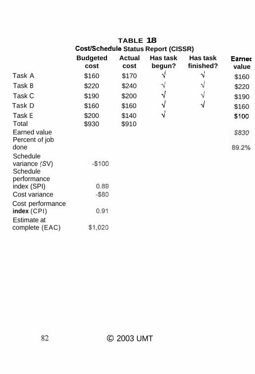
Task A

Task B

Task C Task D

Task E Total Earned value Percent of job done Schedule variance (S V) Schedule performance index (SPI) Cost variance Cost performance index (CPI) Estimate at complete (EAC)

TABLE 18 CostlSchedule Status Report (CISSR) Budgeted Actual Has task Has task

cost cost begun? finished?

$160 $170 4 4 $220 $240 d d $190 $200 4 .\I $160 $160 4 4 $200 $140 4 $930 $910

Earnec value

$160

$220

$190

$1 60

$100

O 2003 UMT

CHAPTER FIVE REAL OPTION APPROACH TO PROJECT DECISION MAKING

Financial investors routinely buy options either to purchase or sell a stock by a certain date (referred to as calls and puts respectively). What options do is to provide investors with time to see how well a stock performs before committing their full resources to purchasing or selling it. For example, for a price of $4.00 a share, you may be able to buy a call option to purchase Globus stock at $60 a share by a given date. If Globus stock rises to $80 a share, you can exercise your option and pocket a respectable profit. If it does not rise sufficiently, you will elect not to exercise the option. Note that use of these options serves a risk management function.

The options approach to investing in stock can be generalized to cover investments in physical assets as well. In this case, you are said to be dealing with real options. For example, managers at a chemical company can view investment in

O 2003 UMT 83

research and development (R&D) as a call option. By carrying out R&D, the managers can gain valuable information on what kind of production line they should build to produce and market the chemical that emerges from the R&D effort. Thus they are in a better position to make a major decision on whether or not to build a new production line, and what it should cost so that it leads to profitable results. By taking a real options perspective on making the R&D investment, they try to determine whether the "price" of the option (i.e., the anticipated R&D expense) is worthwhile in view of the added investment information it provides.

A numerical example helps to clarify how the real option approach can be used to manage the risk associated with selecting projects. Let's say that Globus Enterprises is thinking about expanding its capacity to manufacture the chassis used to house personal computers. The expansion would require building new production facilities. Before launching the expansion project, it would conduct a feasibility study estimated to cost $800,000. Preliminary thinking suggests that Globus should expand in one of three ways: conduct a major expansion at a cost of $6 million, a moderate expansion at a cost of $4 million, or a minor expansion at a cost of $2 million. Is there a market for the additional chassis? The marketing department sees two possible revenue scenarios: a high volume of sales of $6.5 million, and a low volume of sales of $2.5 million. The

@ 2003 UMT

ernatives facing Globus are pictured as a nventional decision tree in Figure 7.

Conduct feasibility study

Figure 7

Cost Revenue

O 2003 UMT

CONVENTIONAL PROFITABILITY ANALYSIS

At this stage, the question Globus management is wrestling with is whether the financial prospects of the potential project are sufficiently good to justify investing $800,000 to conduct a feasibility study. So they carry out a conventional financial analysis to see whether anticipated return on investment justifies spending $800,000 on a feasibility study.

Assuming that the high revenue and low revenue scenarios are equally probable (i.e., the probability of each event is 0.5), expected revenue is:

e(Revenue) = 0.5 x ($6.5 million) + 0.5 x ($2.5 million) = $4.5 million Assuming that major, moderate, and minor

expansion costs are equally probable (i.e., the probability of each event is 0.33), expected cost is:

e(Cost) = 0.33 x ($6 million) + 0.33 x ($4 million) + 0.33 x ($2 million) = $4 million Consequently, expected profit is: e(Profit) = e(Revenue) - e(Cost) = $4.5 million - $4.0 million = $0.5 million

O 2003 UMT

Note that the expected profit of $0.5 million is less than the $800,000 cost for the feasibility study. This means that we will not be able to cover the expense of the feasibility study if we carry out the project.

Verdict: Don't spend money on the feasibility study and don't carry out the project.

With the real option approach, we take a multi-step approach to decision making, where during each step we incorporate newly gained information into the decision analysis. In this example, we begin by estimating the profitability associated with each of the three investment scenarios. The results are:

SCENARIO A.' MNOR EXPANSION

e(Profit1Major expansion) = e(Revenue) - e(Cost1Major expansion) = $4.5 million - 6.0 million = -$I .5 million What these computations tell us is that if we

proceed with an attempt to engage in a major expansion of production capacity after we carry out the feasibility study, we will actually lose money. However, if we know that we will lose money, we will never carry out a major expansion because it does not make sense to go forward with a money losing proposition. Consequently, our expected profit is

O 2003 UMT 87

zero! This is an important point and lies at the heart of the real option approach. What we have done is to use new information - in this case, knowledge that we will lose money by investing in a major expansion - to adjust our thinking about the future prospects of an investment.

SCENARIO 5.' MODERATE EXPANSION

e(Profit1Moderate expansion) = e(Revenue) - e(Cost1Moderate expansion) = $4.5 million - $4.0 million = $0.5 million In this case, the numbers tell us that with

moderate expansion of capacity, we expect to make a modest profit of $500,000.

e(Profit1Minor expansion) = e(Revenue) - e(Cost1Minor expansion) = $4.5 million - $2.0 million = $2.5 million The highest level of profit - $2.5 million -will

be gained by undertaking a modest expansion of capacity.

OVERALL PROFlTAB/LIN

Assuming the probability of encountering each of the three scenarios described above is equal (i.e., the probability being 0.33 in each case), the expected overall profitability is:

O 2003 UMT

e(Profitabi1ity) = 0.33 x ($0.0) + 0.33 x ($0.5 million) + 0.33 x ($2.5 million) = $1.0 million The expected profit of $1.0 million would

more than cover the $800,000 cost of the feasibility study.

Verdict: Spend the $800,000 on the feasibility study, and if Scenario A plays out, don't pursue further investment; if Scenario B plays out, invest in moderate expansion of capacity; and if Scenario C plays out, invest in minor expansion of capacity.

Use of the real option approach need not stop here. Let's assume that Globus goes ahead with the feasibility study whose results lead its management to conclude that engineering and production requirements demand that they build the "moderate expansion" production facility. Meanwhile, the marketing department is carrying out a careful market research study to determine which of the two revenue scenarios is most likely to arise. A question that Globusmanagers must address is: Should the company immediately begin building the new facilities, or should it wait until it has better marketing information?

O 2003 UMT

Using a conventional approach to computing profit:

e(Profit1Moderate expansion) = e(Revenue) - e(Cost1Moderate expansion) = $4.5 million - $4.0 million = $0.5 million

Using a real option approach, Globus takes into account the revenue prospects:

e(Profit1Moderate expansion and high revenue) = e(Revenue1High revenue) - e(Cost1Moderate expansion) = $6.5 million - $4.0 million = $2.5 million In this case, Globus will realize a substantial

profit, and it should certainly proceed with the investment.

e(Profit1Moderate expansion and low revenue) = e(Revenue1Low revenue) - e(Cost1Moderate expansion) = $2.5 million - $4.0 million = -$I .5 million

O 2003 UMT

In this case, Globus will lose money, and it should abandon the investment. Note that if Globus abandons the project, its expected profit is zero, not -$I .5 million.

OVERALL PROFITABILITY

Assuming the probability of realizing the high revenue and low revenue scenarios is equal (i.e., the probability is 0.5 in each instant), the expected overall profitability is:

e(Profit) = 0.5 x ($2.5 million) + 0.5 x ($0.0) = $1.25 million This computation of $1.25 million in expected

profit is greater than the $0.5 million computed using the traditional approach to computing profitability. These results suggest that before proceeding to build the new production facilities, it is worthwhile to wait until the marketing study is complete in order to determine whether anticipated revenue will be substantial enough to justify building the plant.

OTHER CONSIDERATIONS

The example provided here clearly oversimplifies what happens in the real world. For instance, you should recognize that every number used when employing the real option approach is a guess. In our example, the costs associated with the three cost scenarios are guesses. The expected revenues generated in the market place are

O 2003 UMT

guesses. The probabilities of the different outcomes are guesses. Clearly, when applying the real option approach to an actual problem, you need to use the best estimates you can come up with.

Also, in our simplified example, there are two identical pay-off scenarios for each investment situation. In the real world, you will encounter diverse pay-off scenarios. Additionally, in the example, probabilities are assumed to be the same across the three investment scenarios and across the two revenue scenarios. In the real world, the probabilities will differ.

Finally, in this example we have not dealt with an issue that is supremely important in the arena of financial options: timing. When investing in stocks, you have a clearly defined period of time in which to exercise an option. American options allow you to exercise it up to the close-out date, while European options allow you to exercise it on the close-out date. Your decision is governed by your knowledge of the value of the option, which is easy to obtain because stocks are continually traded and have publicly listed purchase prices. If the stock price is high enough, you exercise the option; if not, you do not.

In contrast, real options are not traded in the market place, so their value is not easily determined. This has implications for timing decisions. In our example above, we conclude that before investing in physically building a moderate-cost production line, we should wait until we have more information on

O 2003 UMT

market conditions (i.e., How many chassis do we think we can sell?). But it is not clear how long we should wait. Two months? Six months? A year? There is no definitive answer to this question, given all the uncertainties we face.

It is unlikely that you can use the real option approach mechanically, where you plug various numbers into a formula and come up with clear guidance on what to do. The important thing to bear in mind is the rationale underlying the real option approach. That is, it promotes the making of phased decisions, where you continually embed new information you gain into your assessment of the costs and benefits of future courses of action. It provides a guide for decision making rather than definitive results.

O 2003 UMT

O 2003 UMT

Until recent times, the role of managers on projects was that of implementer. Like a non- commissioned officer in the Army, managers received direction from their superiors, and then set out to achieve the goals that were established for them. In this environment, their principal job was to develop schedules for project efforts, muster resources to do the job, and deliver the goods at the right time.

In the 1990s, this perspective underwent a radical transformation. The pressures of competition, coupled with the increased complexity of products, services, and the work environment, required that the men and women who implement projects be flexible, smart, and independent. The principal skills they needed were business skills, because a project effort was fundamentally a business effort. While the traditional view held them to be non-commissioned officers implementing other people's orders, the new model pictured them as CEOs of little businesses.

To fill the role of business person, managers on projects found that they needed to develop solid financial skills, because their job now required them to deliver project solutions in a cost-effective manner. In analyzing cash inflows and outflows, they were expected to understand and be able to use standard time-value of money techniques, such as

O 2003 UMT

present value, internal rate of return, and payback period analyses. When assessing the merits of projects, they needed to know how to carry out benefit-cost analyses. They also were required to have a grasp of a range of cost estimating techniques, including bottom-up and top-down techniques. Once a project was underway, they were charged with controlling costs, so they were expected to be able to use the earned value management methodology.

There is nothing particularly difficult about the financial perspectives and techniques that managers on projects should master. As with any ability, achievement of proficiency first requires understanding, and then practice, practice, practice. Hopefully, this book has supplied readers with an understanding of the core financial perspectives that managers who work on projects should possess. Ultimately, however, mastery of the tools and techniques requires managers to take what they have learned and apply it routinely on their projects.

O 2003 UMT