INDEGREE PROJECT ELECTRICAL ENGINEERING,SECOND CYCLE, 30 CREDITS

,STOCKHOLM SWEDEN 2017

Predictive vehicle motion control for post-crash scenarios

DÁVID NIGICSER

KTH ROYAL INSTITUTE OF TECHNOLOGYSCHOOL OF ELECTRICAL ENGINEERING

Predictive vehicle motion control

for post-crash scenarios.

David Nigicsernigicser@kth.se

August 31, 2017

Master ThesisAutomatic Control

KTH School of Electrical Engineering

Industrial supervisors:Mustafa Ali Aratmustafa.ali.arat@nevs.comEduardo Simoes da Silvaeduardo.simoes@nevs.com

Academic examiner and supervisor: Jonas Martenssonjonas1@kth.seValerio Turri

turri@kth.se

Abstract

The aim of the project is to design an active safety system forpassenger vehicles for mitigating secondary collisions after an initialimpact. The control objective is to minimize the lateral deviationfrom the known original path while achieving a safe heading angle af-ter the initial collision. A hierarchical controller structure is proposed:the higher layer is formulated as a linear time varying model predic-tive controller that defines the virtual control moment input; the lowerlayer deploys a rule-based controller that realizes the requested mo-ment. The designed control system is then tested and validated inSimulink as well as in IPG CarMaker, a high fidelity vehicle dynamicssimulator.

Keywords:Vehicle Motion Control, Multiple Event Accidents, Secondary CollisionMitigation, Linear Time Varying Model Predictive Control, TorqueVectoring, Sliding Mode Control, NEVS

I

Sammanfattning

Syftet med projektet ar att for personbilar designa ett aktivt sakerhetssystem for att undvika foljdkollisioner efter en forsta kollision. Malet ar att minimera den laterala avvikelsen fran den ursprungliga fardvagen och att samtidigt uppna en saker kurs efter den forsta kol-lisionen. En hierarkisk regulatorstruktur foreslas. Det ovre skiktet i regulatorn ar formulerat som en linjar tidsvarierande modell prediktiv kontroller som definierar den virtuella momentinmatningen. Det nedre skiktet anvander en regelbaserad regulator som realiserar det begarda momentet. Det konstruerade styrsystemet testades och validerades se-dan i Simulink samt i IPG CarMaker, en simulator med hog precision for fordonsdynamik.

Nyckelord:Fordonsstyrning, Rorelsestyrning, Foljdolyckor, Sekundar kollisionsbe-kampning, Linjar Tidsvarierande Modellprediktiv Reglering, Moment-vektorering, Sliding mode-reglering, NEVS

II

Acknowledgements

Firstly, I owe a debt of gratitude to my academic supervisor, Valerio Turri forgiving me thoughtful guidance throughout the whole thesis project. Thankyou for your engagement and patience during our long conversations. Yourconstant feedback and advice has enabled me to reach very high standardswith the project. Also, I would like to thank my academic examiner, JonasMartensson for facilitating and supporting the thesis project from the sideof KTH.

Secondly, I am grateful for the guidance of my industrial supervisors, MustafaAli Arat and Eduardo Simoes da Silva. Your supervision assured the project’srelevance to industry and provided me the perfect ground to grow profes-sionally. It has been a pleasure to work alongside people of the Softwareand Controls department at NEVS, lunch time conversations helped me torelax and stay focused.

I am also very grateful for my friends and colleagues in Goteborg. Nikhil,Hjortur and Anand, it has been a real pleasure to work and share an episodeof my life with you guys. Thank you for all those conversations on the busand train rides, and for your motivation and camaraderie through good daysand bad days. Likewise, I am grateful for your friendship and constant sup-port Paolo. I am glad we made that move to the city which has great thingsin store for us!

Lastly and most importantly, I want to express my deepest appreciation tomy father, mother, sister and brother. Without your unconditional love andselfless support I could not have finished this thesis and my master degree.Thank you for always inspiring and challenging me to fulfil my potential!

Soli Deo gloria

III

List of Figures

2.1 Top view of a vehicle indicating the physical distribution ofimpacts analysed in [9]. . . . . . . . . . . . . . . . . . . . . . 7

3.1 The road-fixed, inertial coordinate system, i.e. global frame,denoted by capitals XY Z. And the vehicle-fixed coordinatesystem, i.e. local frame, denoted by lower-case xyz [ISO 6487]. 12

3.2 Two track model of a vehicle in the XY plane with a referencelane. Original figure taken from B. J. Kim et al. [14]. . . . . 13

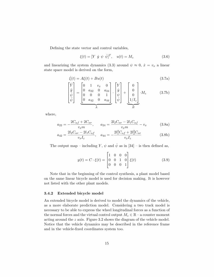
3.3 Simplified semi-empirical Pacejka tire model of equation (3.13),and its modified version in equation (3.14) capturing the non-linear lateral force - tire slip angle relation. . . . . . . . . . . 17

4.1 The proposed hierarchical control architecture. . . . . . . . . 194.2 Open loop vehicle heading angle trajectory - subject to an

impulse of 8 kNs. . . . . . . . . . . . . . . . . . . . . . . . . . 255.1 Illustration of a collision in a generic four-way intersection

between two passenger vehicles [ITE, 2010]. . . . . . . . . . . 275.2 Frequency distribution of impact magnitude by original ve-

locity, presented in [41] . . . . . . . . . . . . . . . . . . . . . . 285.3 Illustration of the crash validation scheme, including the con-

troller activation timing. . . . . . . . . . . . . . . . . . . . . . 295.4 The plant’s global lateral velocity (VY ) and the linearized

(around ψ = 0) prediction model’s lateral velocity - 8 kNsimpact. . . . . . . . . . . . . . . . . . . . . . . . . . . . . . . 31

5.5 Performance of the linear MPC, compared to an SMC scheme- 4 kNs impact. . . . . . . . . . . . . . . . . . . . . . . . . . . 33

5.6 Performance of the linear MPC, compared to an SMC scheme- 8 kNs impact. . . . . . . . . . . . . . . . . . . . . . . . . . . 34

5.7 Longitudinal and lateral tire forces as functions of the longi-tudinal slip ration and tire slip angle. Original plot can befound in Kim et al. [14]. . . . . . . . . . . . . . . . . . . . . . 36

5.8 Comparison of the linear MPC and linear time varying MPCcontrollers - 8 kNs impact. The LTV-MPC is plotted for bothzero and π heading angle references. . . . . . . . . . . . . . . 38

5.9 Vehicle states after an 8 kNs impact simulated in IPG Car-Maker with the LTV-MPC deployed. . . . . . . . . . . . . . . 41

5.10 Longitudinal slip ratios and torque requests on the wheels(motors) after an 8 kNs impact simulated in IPG CarMakerwith the LTV-MPC deployed. . . . . . . . . . . . . . . . . . . 42

IV

5.11 Vehicle trajectories after a 6 and 8 kNs impact simulated inIPG CarMaker with the LTV-MPC deployed. The open looptrajectories are included as a reference. . . . . . . . . . . . . . 43

5.12 Lateral acceleration profiles at 6 kNs and 8 kNs impacts. . . . 44

List of Tables

4.1 Final vehicle heading angles in case of open loop simulation ofcrashes at various initial impulses. Maximum heading angleswhen the control loop is closed, for the same crashes. . . . . . 25

4.2 Solver calculation times in seconds using different QP solversand tracking different heading angle references. The simula-tion time is t = 6 seconds. . . . . . . . . . . . . . . . . . . . . 26

5.1 Performance comparison of the linear MPC and LTV-MPCcontrollers. With the LTV-MPC, two different reference head-ing angle is tracked. . . . . . . . . . . . . . . . . . . . . . . . 37

5.2 IPG CarMaker simulations of different magnitude impacts.The settling time is defined as settling around the referencein a band of ± 10 degrees. . . . . . . . . . . . . . . . . . . . . 40

V

Nomenclature

CoG – Center of GravityDoF – Degrees of FreedomLTV – Linear Time VaryingLTV-MPC – Linear Time Varying Model Predictive ControlMEA – Multiple Event AccidentMPC – Model Predictive ControlMUC – Main Use CaseNEVS – National Electric Vehicle SwedenQP – Quadratic ProgramQLOC – Quasi-linear Optimal ControllerSMC – Sliding Mode Control

VI

Contents

1 Introduction 11.1 Motivation . . . . . . . . . . . . . . . . . . . . . . . . . . . . 11.2 Problem formulation . . . . . . . . . . . . . . . . . . . . . . . 21.3 Thesis contribution . . . . . . . . . . . . . . . . . . . . . . . . 31.4 Outline . . . . . . . . . . . . . . . . . . . . . . . . . . . . . . 3

2 Background 52.1 Post-crash vehicle motion control . . . . . . . . . . . . . . . . 52.2 Vehicle motion control with MPC . . . . . . . . . . . . . . . . 8

3 Vehicle dynamics modelling 123.1 Vehicle coordinate systems . . . . . . . . . . . . . . . . . . . . 123.2 Two track plant model . . . . . . . . . . . . . . . . . . . . . . 123.3 High fidelity vehicle dynamics model - as plant model . . . . 143.4 Prediction models . . . . . . . . . . . . . . . . . . . . . . . . 14

3.4.1 Linearized bicycle model . . . . . . . . . . . . . . . . . 143.4.2 Extended bicycle model . . . . . . . . . . . . . . . . . 15

4 Vehicle motion control 194.1 Architecture of the proposed control system . . . . . . . . . . 194.2 Linear MPC . . . . . . . . . . . . . . . . . . . . . . . . . . . . 19

4.2.1 Cost function . . . . . . . . . . . . . . . . . . . . . . . 204.2.2 Model constraints . . . . . . . . . . . . . . . . . . . . 204.2.3 MPC formulation . . . . . . . . . . . . . . . . . . . . . 21

4.3 Linear Time Varying MPC . . . . . . . . . . . . . . . . . . . 214.3.1 Cost function . . . . . . . . . . . . . . . . . . . . . . . 234.3.2 Model constraints . . . . . . . . . . . . . . . . . . . . 234.3.3 MPC formulation . . . . . . . . . . . . . . . . . . . . . 24

4.4 Reference generation . . . . . . . . . . . . . . . . . . . . . . . 244.5 Implementation strategy . . . . . . . . . . . . . . . . . . . . . 25

5 Experiments 275.1 Definition of the main use case . . . . . . . . . . . . . . . . . 275.2 Linear MPC results . . . . . . . . . . . . . . . . . . . . . . . . 295.3 LTV-MPC results . . . . . . . . . . . . . . . . . . . . . . . . . 35

5.3.1 Performance comparison . . . . . . . . . . . . . . . . . 355.3.2 Simulations with IPG CarMaker . . . . . . . . . . . . 39

5.4 Human factors . . . . . . . . . . . . . . . . . . . . . . . . . . 44

VII

6 Conclusion and further work 456.1 Extensions of the controller architecture . . . . . . . . . . . . 456.2 Extensions of the MPC formulation . . . . . . . . . . . . . . . 46

VIII

1 Introduction

This chapter provides an overview of the problem intended to solve anddescribes its relevance to current industrial trends.

1.1 Motivation

Automotive safety is of vital importance to drivers, passengers, manufactur-ers and society in general. Aiming to guarantee passenger safety at all times,the automotive sector has seen significant technological advancements of thefield in recent years. These safety systems can be categorised as either ac-tive or passive safety systems. Passive safety systems help to guarantee thesafety of the driver and passengers without intervening in vehicle dynamicsthrough actuators, e.g. airbags, seat-belt tensioners and vehicles’ physicalstructure. Active safety systems, however, actively monitor vehicle states toprevent and mitigate the effects of a crash through actuation, e.g. tractioncontrol system, anti-lock braking system and various advanced driver assis-tance systems. In 2016, on the roads of the European Union alone there havebeen 25500 fatal road accidents recorded [1] and this number has displayeda distinct decreasing tendency over the past decade thanks to the introduc-tion of increasingly advanced safety systems. Recent studies have shown areduction of single vehicle accidents of about 50% for vehicles equipped withelectronic stability control systems [20], highlighting the potential of suchsystems.

The increasing concern over sustainability and environmental pollutionalong with the availability of fossil fuels led to a shift in mobility from thepresent traditional internal combustion engines to propulsion with electricmotors. In the last two decades, electrification of automotive powertrainsystems has enabled extended functionalities and more refined active safetysystems. This electrification of chassis and drivetrain systems have led to ahigh degree of over actuation, thus allowing more flexibility in the design ofactive safety systems.

An analysis by Yang et al. shows that approximately 30% of road acci-dents are so called multiple event accidents (MEAs) [2], where the vehicleis subject to more than one harmful event. Statistical studies [24, 25, 26]based on vehicle crash data, indicate that the risk of severe injuries is muchhigher in MEAs than in single event accidents: more than 50% of the MEAsleave occupants with serious injuries. Moreover, a crash analysis report bythe National Highway Traffic Safety Administration [19] investigates the ve-hicle heading angle distribution in MEAs and concludes that the majority of

1

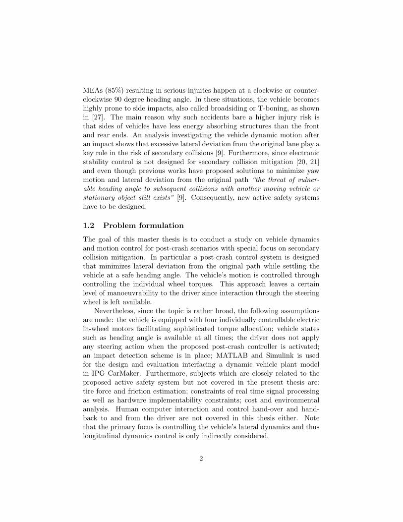
MEAs (85%) resulting in serious injuries happen at a clockwise or counter-clockwise 90 degree heading angle. In these situations, the vehicle becomeshighly prone to side impacts, also called broadsiding or T-boning, as shownin [27]. The main reason why such accidents bare a higher injury risk isthat sides of vehicles have less energy absorbing structures than the frontand rear ends. An analysis investigating the vehicle dynamic motion afteran impact shows that excessive lateral deviation from the original lane play akey role in the risk of secondary collisions [9]. Furthermore, since electronicstability control is not designed for secondary collision mitigation [20, 21]and even though previous works have proposed solutions to minimize yawmotion and lateral deviation from the original path “the threat of vulner-able heading angle to subsequent collisions with another moving vehicle orstationary object still exists” [9]. Consequently, new active safety systemshave to be designed.

1.2 Problem formulation

The goal of this master thesis is to conduct a study on vehicle dynamicsand motion control for post-crash scenarios with special focus on secondarycollision mitigation. In particular a post-crash control system is designedthat minimizes lateral deviation from the original path while settling thevehicle at a safe heading angle. The vehicle’s motion is controlled throughcontrolling the individual wheel torques. This approach leaves a certainlevel of manoeuvrability to the driver since interaction through the steeringwheel is left available.

Nevertheless, since the topic is rather broad, the following assumptionsare made: the vehicle is equipped with four individually controllable electricin-wheel motors facilitating sophisticated torque allocation; vehicle statessuch as heading angle is available at all times; the driver does not applyany steering action when the proposed post-crash controller is activated;an impact detection scheme is in place; MATLAB and Simulink is usedfor the design and evaluation interfacing a dynamic vehicle plant modelin IPG CarMaker. Furthermore, subjects which are closely related to theproposed active safety system but not covered in the present thesis are:tire force and friction estimation; constraints of real time signal processingas well as hardware implementability constraints; cost and environmentalanalysis. Human computer interaction and control hand-over and hand-back to and from the driver are not covered in this thesis either. Notethat the primary focus is controlling the vehicle’s lateral dynamics and thuslongitudinal dynamics control is only indirectly considered.

2

The present thesis investigates weather model predictive control (MPC)is a suitable higher layer controller in a hierarchical controller architectureto provide control inputs in the described post-crash vehicle motion controlproblem.

1.3 Thesis contribution

The present thesis work contains the following contributions:

� Vehicle dynamics modelling. Constructing both plant and predictionmodels tailored to the introduced problem.

� Formulation and implementation of linear and linear time varyingmodel predictive controllers.

� Controller performance analysis and validation. Extensive simulationsof the proposed active safety system, validating control objectives.

This master thesis has been carried out at National Electric Vehicle Swe-den (NEVS) in Trollhattan, Sweden. Given the rather broad topic, somespecific parts of the proposed active safety system have been investigatedby myself, others by Nikhil Jain, a peer student of mine. Nikhil’s main con-tribution is the elaboration of an alternative controller for the post impactvehicle motion control problem, namely a sliding mode controller (SMC)[39]. This means that the project’s framework has been developed as a jointeffort and is therefore common in both reports. Specifically, the followingconcepts have been developed in collaboration: the control objective, defi-nition of the main use case, vehicle dynamic plant models, impact injectionand controller activation schemes. Nevertheless, these common parts havedifferent significance in the two reports and have been documented individ-ually, and thereby, non of the chapters or sections are an exact copy of eachother in the two master thesis reports.

1.4 Outline

In chapter 2 an overview of the theoretical background of the formulatedproblem is described. Chapter 3 contains a set of vehicle dynamics models.After the introduction of a three degrees of freedom (DoF) two track plantmodel and the fourteen DoF IPG CarMaker plant model is briefly described.The same chapter contains the description of two prediction models: a sim-ple, augmented two DoF linear bicycle model and a more elaborate, three

3

DoF extended bicycle model. Chapter 4 introduces the proposed controllerarchitecture and elaborates the design of the linear MPC and the linear timevarying MPC (LTV-MPC) controllers. In chapter 5, the main use case isdefined and the sequence of simulations is described. This chapter also de-scribes the main design decisions and the necessity of the more sophisticatedLTV-MPC formulation. Last, chapter 6 contains the conclusions and detailspossible further extensions of the project.

4

2 Background

This chapter is an overview of various vehicle dynamics and motion controlproblems, focusing on the proposed control architectures and approaches aswell as torque allocation. Primarily the focus is on problems with similarassumptions to this thesis. First, an overview of various post-crash stabilitycontrollers is given. Second, relevant vehicle dynamics control problems arereviewed, focusing on solutions utilizing MPC in particular.

2.1 Post-crash vehicle motion control

Sakai et al. [3] propose a novel robust dynamics yaw-moment control system,describing a vehicle attitude control method generating yaw from torquedifferences between the left and right wheels, assuming four independentlydriven in-wheel motors. The described controller is a robust-model matchingcontroller based on linear-quadratic regulator theory using state feedback.Through simulations, the authors identified stability problems on low fric-tion roads, due to saturated traction tire force and therefore propose a new,robust skid detection method which does not require wheel and chassis lon-gitudinal velocities. Instead, observing the ratio of tractive force and motortorque (the slope of the traction force - motor torque curve) wheel skid-ding is classified. Simulations then show that skids during cornering aresuccessfully suppressed.

An adaptive stability control system is proposed by Wang et al. [6] to ad-dress the reference tracking problem of a four-wheel independently actuatedelectric vehicle. A hierarchical controller structure is designed where boththe longitudinal speed and yaw rate are controlled simultaneously. Thehigher layer, an analytical nonlinear control approach using a Lyapunovfunction, calculates a virtual total ground force request and the force splitbetween the left and right sides of the vehicle. The lower layer distributesthe higher layer’s control efforts to the four wheels, using a numerical opti-mization based control allocation algorithm.

Yoshimoto et al. investigate the deactivation conditions of a vehiclestability assistance system in a study [4], based on a two wheel nonlinearvehicle model and a linear-quadratic regulator realizing active steering. Aninstantaneous yaw rate is injected in simulation to the vehicle travellingat a constant speed testing seven different deactivation timings, both on astraight and curved course. The analysis concludes that a latency time isnecessary before the assistance system returns control to the driver. Thislatency time however, depends on the drivers’ skills.

5

A hierarchical stability controller, utilizing direct yaw moment controltechnique is investigated on a four-wheel independently actuated electric ve-hicle by Song et al. [28]. The authors propose a novel sliding mode control(SMC) technique for the motion control problem, tracking a desired, ref-erence vehicle motion. The SMC is deployed as the higher layer, trackingboth the yaw rate and sideslip where the sliding surface is defined as theweighted combination of the yaw rate and sideslip angle errors. The calcu-lated total driving force and yaw moment requests are the inputs of the lowerlayer, distributing individual wheel torques considering adhesion limits andactuator constraints, formulated as an optimization problem. The designedcontrol system is tested in a lane-change manoeuvre in simulation. Resultsshow improved reference tracing and steerability while meeting the designrequirements. For post-crash vehicle motion control however, yaw rate anddriving torque reference generation is a crucial question.

In [29], Kim et al. propose a preemptive steering control strategy, cal-culating a counter-steering action by a feedforward and feedback controller,attenuating vehicle motion after an external impact based on the predictedcollision strength. Here, the sliding mode control concept is applied, drivingboth lateral velocity and yaw rate to the reference. For actuation, differen-tial braking is considered, stabilizing the vehicle post impact, using a simplerule based approach.

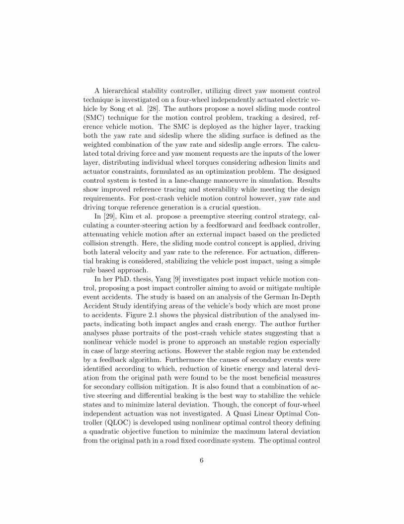
In her PhD. thesis, Yang [9] investigates post impact vehicle motion con-trol, proposing a post impact controller aiming to avoid or mitigate multipleevent accidents. The study is based on an analysis of the German In-DepthAccident Study identifying areas of the vehicle’s body which are most proneto accidents. Figure 2.1 shows the physical distribution of the analysed im-pacts, indicating both impact angles and crash energy. The author furtheranalyses phase portraits of the post-crash vehicle states suggesting that anonlinear vehicle model is prone to approach an unstable region especiallyin case of large steering actions. However the stable region may be extendedby a feedback algorithm. Furthermore the causes of secondary events wereidentified according to which, reduction of kinetic energy and lateral devi-ation from the original path were found to be the most beneficial measuresfor secondary collision mitigation. It is also found that a combination of ac-tive steering and differential braking is the best way to stabilize the vehiclestates and to minimize lateral deviation. Though, the concept of four-wheelindependent actuation was not investigated. A Quasi Linear Optimal Con-troller (QLOC) is developed using nonlinear optimal control theory defininga quadratic objective function to minimize the maximum lateral deviationfrom the original path in a road fixed coordinate system. The optimal control

6

Figure 2.1: Top view of a vehicle indicating the physical distribution ofimpacts analysed in [9].

problem is formulated as a two-point boundary value problem (2pt-BVP)and it is fully determined by the active force and moment constraints of thesystem. The designed controller is verified in various test scenarios compar-ing to a generic post impact braking controller [10] as well as to a simpleanti-lock brake system. It is found that the maximum lateral deviation canbe considerably reduced when the QLOC is deployed as compared to thepost impact braking function, significantly outperforming cases when onlythe anti-lock brake system intervenes.

An accident statistical study performed by the German Insurance As-sociation confirms that even vehicles involved in a light impact are highlylikely to experience a severe secondary crash and a third of all accidentswith severe injuries consist of multiple events [18].

In a paper by Zhou et al. [5], vehicle stabilization in response to exoge-nous impulsive disturbances is studied. The authors propose a post-impactstabilizing controller with the objectives to attenuate sideslip angle, yaw rateand roll rate immediately after a crash disturbance, recovering vehicle sta-bility. The controller is assumed to have access to all necessary vehicle statesand it is based on a planar two track three DoF vehicle model. The con-troller is an extension of sliding mode control theory, using multiple slidingsurface theory. A detailed crash detection and validation scheme is intro-duced, monitoring the rate of change of certain vehicle states. When above

7

an empirical threshold for three consecutive sampling intervals, the controlsystem is activated triggering a validation scheme to avoid misdetection. Toevaluate controller performance, the proposed system is tested against threedifferent control approaches (differential braking, differential braking withactive steering, full braking without steering action) in simulation subjectto the same impulsive disturbances. Results show that the proposed con-troller can effectively recover post-event vehicle stability outperforming allthe other approaches.

In a follow-up study, Kim et al. [13] propose a post-impact vehiclestability control system that controls both heading angle and path lateraldeviation to mitigate the severity of secondary crashes. Consequently, theproposed system predicts the heading angle after a collision and controls ve-hicle spin to reach a safe heading angle, defined as multiples of 180 degrees.The proposed method relies on the following assumptions: the event occurson a straight road, only two vehicles are involved and the sensors and actu-ators are fully functioning after the crash. Relying on a collision model forvehicle motion prediction [12], magnitude and location of impulses can beestimated. This calculated impact force is then used to predict the vehicle’smotion. Vehicle side slip angles up to 360 degrees are studied, consider-ing tire characteristics based on Pacejka’s Magic Formula [17], concludingthat significant yaw rate reduction can be achieved when the heading an-gle crosses 180 and 360 degrees. The control synthesis is formulated as anoptimization problem using gradient descent with an objective function min-imizing lateral deviation from the path while achieving the desirable headingangle. Control inputs – longitudinal slip ratios – are obtained by minimizingthe objective function under the slip ratio constraints. The authors arguethat reducing yaw rate as quickly as possible might not be the safest sec-ondary collision mitigation approach, due to the fact that the vehicle is verysensitive to side impacts, hence considering safe heading angles is crucial.Safe heading angles in a post-crash scenario might be determined by thevehicles perception of its surrounding and extensive simulations.

2.2 Vehicle motion control with MPC

Lately, model predictive control has gained popularity in the control com-munity thanks to its attractive features and the availability of faster andfaster embedded platforms. Numerous research fields apply the conceptwith increasing success, including the field of vehicle dynamics and motioncontrol.

8

Model predictive control is a model based, online, constrained finite hori-zon optimization method, capable of handling nonlinear time-varying mod-els and constraints systematically [33], optimizing future plant behaviour.Despite its considerably heavy computational burden [34], nonlinear MPCis a very attractive control technique, especially in applications where theprocess is required to work in wide operating regions and close to the bound-ary of admissible states and inputs [35]. To ease the computational burden,MPC formulation based on successive online linearization of the nonlinearplant model is commonly used, leading to a linear time varying model pre-dictive control formulation. By linearizing the prediction model before eachMPC optimization step the nonlinear MPC problem is transformed intoa LTV-MPC problem, yielding simpler optimization problems in real-time[36].

Controlling an active front steering system of an autonomous vehicle ispresented in [34] by Falcone et al. A known trajectory is followed on a slip-pery road at the highest possible entry speed. Two different methods arepresented, first using a three DoF nonlinear vehicle plant model, formulat-ing a nonlinear MPC problem. The second method is based on successiveonline linearization of the plant model, formulating an LTV-MPC problem.The performance of the two controllers is tested in a double lane-changemanoeuvre. Results show that with both formulations the manoeuvre issuccessfully executed, stabilising the vehicle up to an entry speed of 21 m/son snow covered roads. From a computational point of view, the superiorityof the LTV-MPC formulation is apparent.

A follow-up study of the above publication is carried out by Falcone etal. [35] using the LTV-MPC approach on the integrated vehicle dynamicsproblem in autonomous systems. Here, in addition to active steering, ac-tive braking and active differentials are controlled, calculating the optimalcombination of front steering angle, brake and tractive force inputs to bestfollow a desired trajectory on slippery roads at certain entry speeds. TheLTV dynamics is derived based on a three DoF two track vehicle model,assuming constant normal tire load and using a nonlinear tire model. Thecontroller is again tested in a double lane-change manoeuvre showing anoverall good tracking of the desired path. Moreover, the current formula-tion displays better tracking performance without slowing down the vehicleexcessively.

In a further, extended publication [36], Falcone et al. investigate thestability of LTV-MPC formulation applied to active steering systems. Evenunder no model mismatch, the stability of this control scheme is difficult toprove. The authors introduce a sufficient condition for the uniform asymp-

9

totic stability of the of the origin of the closed-loop system. The proposedcondition is validated in the active front steering problem. Results show con-sistency with what can be achieved by an ad hoc MPC scheme developedby experts of the process.

Turri et al. address lane keeping and obstacle avoidance on low curva-ture roads (e.g. highways) based on linear MPC control architecture [15].First the lateral vehicle dynamics is derived as a function of the longitudinalbraking or acceleration profile, based on an extended bicycle model underthe assumption of the road’s large curvature radius. Expressing the lateraltire forces, the nonlinear semi empirical Pacejka formula [17] is used. Thenonlinear expression, for a given braking ratio, is bounded by two linearfunctions accounting for a conservative and a overreacting lateral dynamics.Based on this, a conservative and an overreacting lateral dynamics modelis derived. The proposed control architecture consist of: longitudinal pro-files generation; parallel MPC problems and post-computation. The MPCformulation predicts the vehicle’s motion using both dynamics models. Forthe state prediction the conservative lateral dynamics model plays the mainrole both in cost function and constraints. The overreacting lateral dynam-ics model represents an auxiliary role, with a shorter prediction horizon.The post-computation block evaluates both cost functions and returns theoptimal braking ratio and the corresponding steering rate with the minimalcost. Hardware-in-the-loop simulations avoiding one and two consecutiveobstacles show the effectiveness of solving the low complexity sub-problems,allowing real-time implementation with long prediction horizons.

In a follow-up publication by Kim et al. [14] the same vehicle motioncontrol problem is approached as in [13]. Here an LTV-MPC is formulatedas higher layer in a hierarchical control architecture. Based on a three DoFvehicle plant model, a six-state nonlinear first-order system is formulated,considering differential braking as actuation. Taking tire saturation con-straints of Pacejka’s Magic Formula tire model [17] into consideration, alinear time varying model is derived, formulating an LTV-MPC controllerfor the control task. The nonlinear vehicle model is successively linearizedusing Taylor series expansion around non equilibrium-operating points, for-mulating quadratic programs (QPs) to set up the optimization. With thismethod, the nonlinear design problem is decomposed into several linear sub-problems. MPC then finds a cost-minimizing control sequence over the pre-diction horizon, while it incorporates feasible control bounds. The proposed,overall hierarchical control structure consists of four functional blocks. Thefirst block compares the desired states with the current states. Then inthe second block, representing the higher layer, the LTV-MPC determines

10

a desired virtual controls input. The third block maps the virtual controldemand onto individual wheel break forces, acting as the lower layer, by anoptimal control allocation process using least-squares. In the fourth block,the actuators manipulate actual physical variables to achieve the desired tireforces. The control objective is to minimize both the lateral deviation fromthe original course and to achieve a safe heading angle while minimizingcontrol efforts. Hence the cost function is defined as the sum of weightedstate deviation and the sum of the weighted control input sequence. Thedesired states are predetermined by off-line optimal computation, determin-ing safer heading angle which minimizes the lateral deviation for the giveninitial impact. This paper relies on differential braking as actuation, so theoutputs of the allocation module (lower layer) are longitudinal wheel brakeforces of each tire. The module aims to find the optimal control input toachieve the virtual control sequence. Based on Pacejka’s Magic tire model[17], the longitudinal tire forces are mapped onto lateral forces, expressed bya linear equation. To validate the proposed control system, simulations inCarSim software were carried out. It is considering two cars with an initiallongitudinal velocity of 30 m/s in a collision with a given initial condition:lateral velocity of 5 m/s, heading angle of 9.2 degrees and yaw rate of 114.6deg/s. During the crash no sensor or actuator failure is assumed. The sam-pling time of the discrete time system is 0.01 seconds, the sampling time forevery linearization of the MPC is set to 0.2 seconds, and the horizon is 20steps, predicting 4 seconds ahead in time. First, the vehicle trajectories incase of four different control strategies are compared. The results suggestthat the vehicle with the proposed control strategy settles into a safe finalheading angle – 180 degrees in this use case – and returns to its original lane,as opposed to the vehicles with other control strategies which show largerlateral deviations from the original lane and are subject to broadsiding byvehicles in other lanes. The robustness of the control system is analysed byrunning the simulations with different initial yaw rate and initial headingangle, corresponding to different magnitudes of the initial impact. On thewhole, the proposed control system minimizes maximum lane deviation andbrings the vehicle back to the original lane with a favoured heading angle of180 or 360 degrees.

11

3 Vehicle dynamics modelling

This chapter presents the mathematical description of the vehicle dynamicswhich is later used as a plant for controller design. The vehicle coordinatesystems are also introduced in brief.

3.1 Vehicle coordinate systems

As one of the control objectives is to minimize post-crash lateral deviationfrom the original path, a road-fixed, inertial coordinate system – referredto as global frame – and a vehicle-fixed coordinate system – referred to aslocal frame – are defined, according to Figure 3.1. Throughout this thesisthe local frame is fixed to the vehicle’s center of gravity (CoG) where thethe x coordinate vector denotes the longitudinal and the y coordinate vectordenotes the lateral directions. The global frame is fixed to the road where Xand Y denote the global longitudinal and lateral directions. Consequently,the yaw angle ψ denotes the vehicle’s heading angle, coinciding in the twoframes.

Figure 3.1: The road-fixed, inertial coordinate system, i.e. global frame,denoted by capitals XY Z. And the vehicle-fixed coordinate system, i.e.local frame, denoted by lower-case xyz [ISO 6487].

3.2 Two track plant model

The equations of motion of a planar, two track vehicle model is derivedusing Newton’s law of motion, based on [14], in the global frame, where thesteering wheel angle is assumed to be zero, i.e. δ = 0. A schematic drawing

12

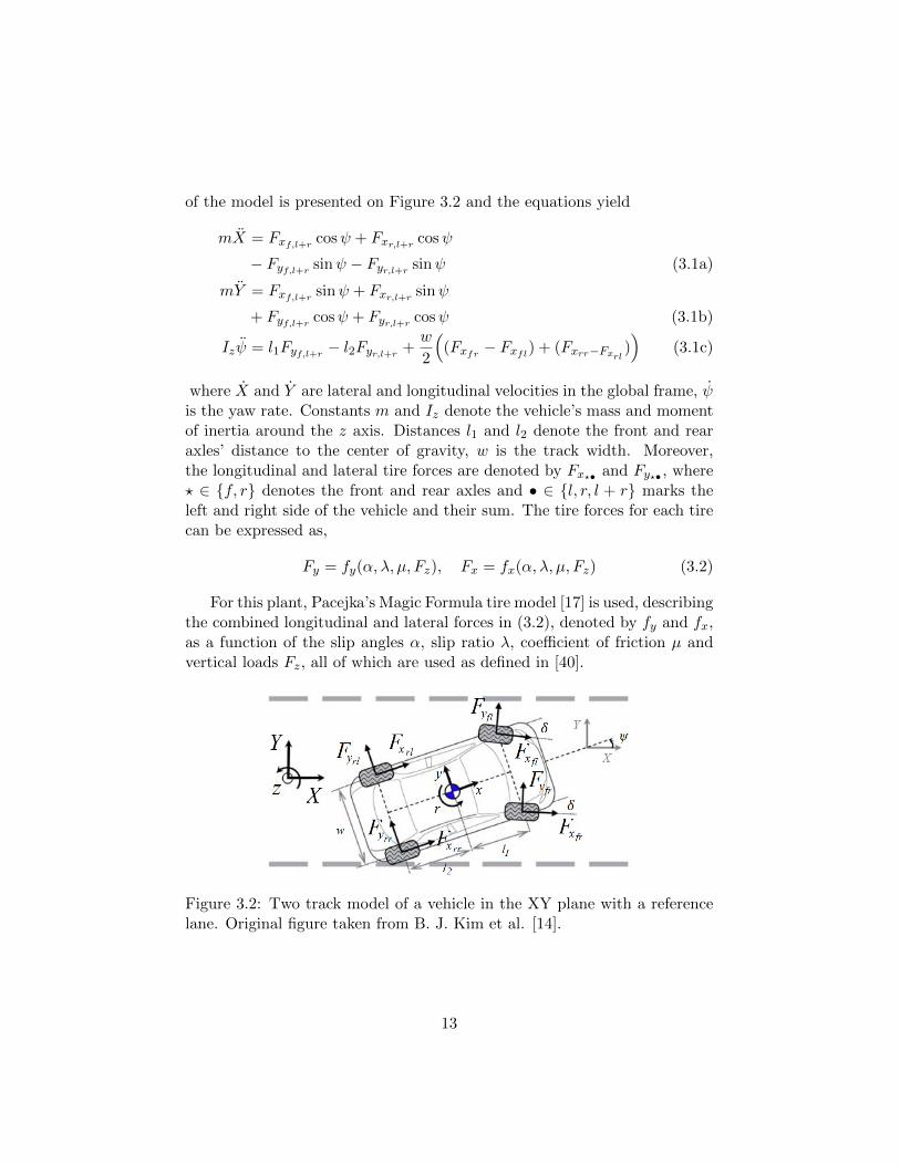
of the model is presented on Figure 3.2 and the equations yield

mX = Fxf,l+rcosψ + Fxr,l+r

cosψ

− Fyf,l+rsinψ − Fyr,l+r

sinψ (3.1a)

mY = Fxf,l+rsinψ + Fxr,l+r

sinψ

+ Fyf,l+rcosψ + Fyr,l+r

cosψ (3.1b)

Izψ = l1Fyf,l+r− l2Fyr,l+r

+w

2

((Fxfr − Fxfl) + (Fxrr−Fxrl

))

(3.1c)

where X and Y are lateral and longitudinal velocities in the global frame, ψis the yaw rate. Constants m and Iz denote the vehicle’s mass and momentof inertia around the z axis. Distances l1 and l2 denote the front and rearaxles’ distance to the center of gravity, w is the track width. Moreover,the longitudinal and lateral tire forces are denoted by Fx?• and Fy?• , where? ∈ {f, r} denotes the front and rear axles and • ∈ {l, r, l + r} marks theleft and right side of the vehicle and their sum. The tire forces for each tirecan be expressed as,

Fy = fy(α, λ, µ, Fz), Fx = fx(α, λ, µ, Fz) (3.2)

For this plant, Pacejka’s Magic Formula tire model [17] is used, describingthe combined longitudinal and lateral forces in (3.2), denoted by fy and fx,as a function of the slip angles α, slip ratio λ, coefficient of friction µ andvertical loads Fz, all of which are used as defined in [40].

Figure 3.2: Two track model of a vehicle in the XY plane with a referencelane. Original figure taken from B. J. Kim et al. [14].

13

3.3 High fidelity vehicle dynamics model - as plant model

A 14 degrees of freedom vehicle model, defined in IPG CarMaker [42] isused for simulations. Components such as the chassis, tires, powertrain,suspension, vehicle aerodynamics are modelled in detail. Hence, this modelaccurately represents the dynamics of a vehicle and therefore provides resultsclose to reality.

3.4 Prediction models

To exploit the predictive power of dynamic models two different vehiclemodels are used as prediction models of the MPC. This section first describesa very simple bicycle model, linearized around a specific working point andusing a linear approximation of the tire dynamics, used in the linear MPCformulation. Then a more complex, extended bicycle model is derived witha nonlinear tire model, which is used in the LTV-MPC formulation.

3.4.1 Linearized bicycle model

A rather simple 2 DoF bicycle model is derived, based on [8] where theequations of motion in the local frame are written as,

my = −mxψ + Fyf + Fyr (3.3a)

Izψ = l1Fyf − l2Fyr +Mz (3.3b)

where y is the lateral velocity and ψ denotes the yaw rate. Constants mand Iz are the vehicle’s mass and moment of inertia around the z axis. Mz isthe virtual control moment input around the z axis. The lateral tire forcesare denoted by Fy? and are calculated by a static, linear approximation ofthe tire dynamics,

Fy? = Cα?α? (3.4)

where Cα? denotes the corresponding cornering stiffness parameters [8] and? ∈ {f, r} denotes the front and rear axles, just as before and α? is thecorresponding slip angle defined by equation (3.12). Note that x = vx isconsidered to be constant, thus the lateral dynamics is not directly consid-ered.

The system dynamics is augmented with the global frame’s lateral dy-namics, which is then later included in the control problem’s minimization,

Y = x sinψ + y cosψ (3.5)

14

Defining the state vector and control variables,

ξ(t) = [Y y ψ ψ]T , u(t) = Mz (3.6)

and linearizing the system dynamics (3.3) around ψ ≈ 0, x = vx a linearstate space model is derived on the form,

ξ(t) = Aξ(t) +Bu(t) (3.7a)Yy

ψ

ψ

=

0 1 vx 00 a22 0 a24

0 0 0 10 a42 0 a44

︸ ︷︷ ︸

A

·

Yyψ

ψ

+

000

1/Iz

︸ ︷︷ ︸

B

·Mz (3.7b)

where,

a22 = −2Cαf + 2Cαr

vxm, a24 =

2l2Cαr − 2l1Cαfvxm

− vx (3.8a)

a42 =2l2Cαr − 2l1Cαf

vxIz, a44 = −

2l21Cαf + 2l22CαrvxIz

(3.8b)

The output map – including Y , ψ and ψ as in [34] – is then defined as,

y(t) = C · ξ(t) =

1 0 0 00 0 1 00 0 0 1

ξ(t) (3.9)

Note that in the beginning of the control synthesis, a plant model basedon the same linear bicycle model is used for decision making. It is howevernot listed with the other plant models.

3.4.2 Extended bicycle model

An extended bicycle model is derived to model the dynamics of the vehicle,as a more elaborate prediction model. Considering a two track model isnecessary to be able to express the wheel longitudinal forces as a function ofthe normal forces and the virtual control output Mz ∈ R – a counter momentacting around the z axis. Figure 3.2 shows the diagram of the vehicle model.Notice that the vehicle dynamics may be described in the reference frameand in the vehicle-fixed coordinates system too.

15

The equations of motion, expressed in the local frame, assuming zerosteering wheel angle (δ = 0) can be written as [34],

mx = myψ + Fxfl + Fxfr + Fxrl + Fxrr (3.10a)

my = −mxψ + Fyfl + Fyfr + Fyrl + Fyrr (3.10b)

Izψ = l1(Fyfl + Fyfr)− l2(Fyrl + Fyrr) +Mz (3.10c)

where x and y are the lateral and longitudinal velocities in the local frame,ψ is the yaw rate. Constants m and Iz denote the vehicle’s mass and mo-ment of inertia around the z axis. The front and rear axles’ distance tothe center of gravity is denoted by l1 and l2 respectively. Mz represents thecontroller action, a virtual moment. Furthermore, Fx?• and Fy?• denote thelongitudinal (or ”tractive”) and lateral (or ”cornering”) tire forces, where? ∈ {f, r} denotes the front and rear axles and • ∈ {l, r} marks the left andright side of the vehicle.

The vehicle’s equations of motion in the global frame [34] are, as inequation (3.5),

X = x cosψ − y sinψ, Y = x sinψ + y cosψ (3.11)

The slip angles – at zero steering wheel angle – of the front and rearwheels can be expressed as,

αf =y + l1ψ

x, αr =

y − l2ψx

(3.12)

Due to the fact that the aim is to control the vehicle’s motion in emer-gency situations, the nonlinear behaviour of the tires is essential to be mod-elled. Therefore, the commonly used linear approximation of the tire dy-namics – as in equation (3.4) – is not suitable in this study. Hence a moresophisticated model, the simplified semi-empirical Pacejka formula [15], [17]is used,

Fy?• =√

(µFz?•)2 − F 2x?• sin(C arctan(Bα?)) (3.13)

where B and C are tire parameters, namely the stiffness factor and theshape factor respectively. The coefficient of friction is assumed to be onei.e. µ = 1.

This tire model captures the saturation of the lateral forces, however,for extremely large slip angles – around 90 degrees, which appear when the

16

-180 -90 0 90 180Slip angle, [deg]

-2000

-1000

0

1000

2000

3000

Late

ral f

orce

, Fy [N

]

arctan(B*sin( ))arctan(B* )

Figure 3.3: Simplified semi-empirical Pacejka tire model of equation (3.13),and its modified version in equation (3.14) capturing the nonlinear lateralforce - tire slip angle relation.

vehicle is spinning – it fails to handle the true behaviour of the slip angle.Thus a slightly modified version of the above Pacejka model is used, on theform of,

Fy?• =√

(µFz?•)2 − F 2x?• sin(C arctan(B sin(α?))) (3.14)

The difference between the two models is demonstrated on Figure 3.3.Note that the stiffness factor and shape factor influence the slope and sat-uration values of the function respectively, and can be identified from theslip curve of the plant.

The vertical load on each tire is assumed to be static, hence not account-ing for the effects of roll and pitch. Rather, the vertical loads are calculatedas a split between the front and rear axle, proportional to the axles’ distancesto the center of gravity [35],

Fzf• =l2

l1 + l2· mg

2, Fzr• =

l1l1 + l2

· mg2

(3.15)

where g denotes the gravitational constant.The longitudinal tire forces are expressed based on the rule-based low

level torque allocation strategy [38]. The virtual control input is first splitbetween the front and rear axle,

Mz = Mzf +Mzr (3.16)

17

and

Mzf =2FzfFztotal

Mz, Mzr =2FzrFztotal

Mz (3.17)

On each axle then, the requested torque is divided onto the left and rightwheels, thus the longitudinal forces can be calculated using Fzfl = Fzfr =12Fzf as,

Fxfl = −2Mzf

w·

FzflFzfl + Fzfr

= −Mzf

w(3.18)

where w denotes the track width of the vehicle.The remaining longitudinal forces can similarly be expressed, yielding,

Fxfr =Mzf

w, Fxrl = −Mzr

w, Fxrr =

Mzr

w(3.19)

With the above expressions, the lateral forces Fyfl , Fyfr , Fyrl and Fyrrcan be expressed from equation (3.14). Using the equations (3.10) – (3.19),the nonlinear vehicle dynamics can be described with the following compactequation [35],

ξ(t) = f(ξ(t), u(t)

)(3.20a)

η(t) = h(ξ(t)

)(3.20b)

where the state vector and input are ξ(t) = [x, y, ψ, ψ, Y,X]T and u(t) = Mz

respectively. f : R6 × R → R6 is the update function and the origin of thestate space is an equilibrium point. The output map – including ψ, ψ andY [34] – is given by,

h(ξ(t)) = hA · ξ(t) =

0 0 1 0 0 00 0 0 1 0 00 0 0 0 1 0

ξ(t) (3.21)

In the present chapter three separate mathematical descriptions of a roadvehicle are presented. In this thesis, these models are either used as a plantmodel or as a prediction model.

18

4 Vehicle motion control

This chapter describes the design process of the active safety system forpassenger vehicles, mitigating secondary collisions after an initial impact.As stated in chapter 1, the control objective is to minimize path lateraldeviation while achieving safe heading angles.

4.1 Architecture of the proposed control system

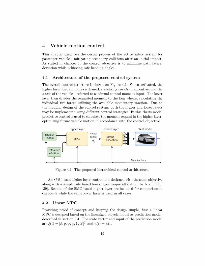
The overall control structure is shown on Figure 4.1. When activated, thehigher layer first computes a desired, stabilizing counter moment around thez axis of the vehicle – referred to as virtual control moment input. The lowerlayer then divides the requested moment to the four wheels, calculating theindividual tire forces utilizing the available momentary traction. Due tothe modular design of the control system, both the higher and lower layersmay be implemented using different control strategies. In this thesis modelpredictive control is used to calculate the moment request in the higher layer,optimizing future vehicle motion in accordance with the control objective.

Figure 4.1: The proposed hierarchical control architecture.

An SMC based higher layer controller is designed with the same objectivealong with a simple rule based lower layer torque allocation, by Nikhil Jain[39]. Results of the SMC based higher layer are included for comparison inchapter 5 while the same lower layer is used in all cases.

4.2 Linear MPC

Providing proof of concept and keeping the design simple, first a linearMPC is designed based on the linearized bicycle model as prediction model,described in section 3.4. The state vector and input of the prediction modelare ξ(t) = [x, y, ψ, ψ, Y,X]T and u(t) = Mz.

19

Discretizing system (3.7) using zero order hold with fixed sampling time∆t yields,

ξ(k + 1) = Adξ(k) +Bdu(k) (4.1)

representing the discrete time linear approximation for a time horizon k =t, ..., t+N . Where matrices Ad and Bd are calculated [32] as,

Ad = eA∆t, Bd =

ˆ ∆t

0eAsB ds (4.2)

where matrices A and B are defined in equation (3.7) and the superscript drefers to representation in discrete time.

4.2.1 Cost function

Consider the quadratic cost function defined as,

VN(ξ(t), U(t), ψref

)=

N∑i=1

(q1Y

2k + q2(ψk − ψref)

2 + q3ψ2k

)+

N−1∑i=0

Ru2t+i,t +

N−1∑i=0

S∆u2t+i,t (4.3)

where U(t) = [ut,t, ..., ut+N−1,t] and ψref are the optimization vector andconstant reference state, respectively. N denotes both the prediction horizonand the control horizon. R and S are weighting matrices of appropriatedimensions and q1, q2 and q3 are weighting scalars. The first summand inequation (4.3) reflects the desired performance on reference tracking, thesecond and third summands are a measure of virtual counter moment effortpenalizing both the control input and control input rate.

4.2.2 Model constraints

Considering the average deceleration of a passenger vehicle while emergencybraking – denoted by adec – and applying Newton’s second law, the totalbraking force yields,

Fbraking = m · adec (4.4)

where m denotes the vehicle’s mass. Meaning an average braking force ofFbraking/4 at each wheel.

Then, considering full braking torque on one side of the vehicle (e.g.both front and rear right wheels) and full propulsive torque on the other side

20

(assuming that approximately similar propulsive longitudinal forces can begenerated), the generated moment around the CoG gives the constraint,

|uk| = |4 · Fbraking/4 · w/2| ≤ umax (4.5)

where w denotes the track width.The constraint on the rate of control input change, namely the slew

rate constraint has been chosen to reflect actuator constraints suggested byNEVS professionals, expressed as,

|ut+1 − ut|∞ ≤ slew (4.6)

The optimization is also subject to the state dynamics constraint, ensur-ing appropriate state evolution according to equation (4.1). Note that nostate constraints have been used in the optimization.

4.2.3 MPC formulation

The following problem is then considered,

minimize VN (ξt, Ut, ψref )subject to ξk+1 = Adξk +Bduk

|uk| ≤ umax|ut+1 − ut|∞ ≤ slew

(4.7)

The optimization yields the optimal input sequence U∗t =[u∗t,t, ..., u

∗t+N−1,t] over the prediction horizon, predicted at time t. Then the

first element of U∗t ,u(t, ξ(t)

)= u∗t,t (4.8)

is applied to the system (3.1). The same calculation is repeated in all con-secutive steps, iteratively. Note that since VN is a convex quadratic functionand both the model and the constraints are linear, this MPC problem canbe formulated as a quadratic program [33].

4.3 Linear Time Varying MPC

Formulation of the LTV-MPC is presented in this section, describing thelinearization and discretization process of the prediction model.

In order to derive the system’s LTV model, the nonlinear vehicle dy-namic equations first have to be linearized around a state trajectory ξ0

21

(non-equilibrium points), where this state trajectory is obtained by apply-ing the input sequence u(k) = u0 for k ≥ 0 (k ∈ N is an arbitrary discretepoint in time), to system (3.20) with ξ(0) = ξ0, i.e [35],

ξ0(t+ 1) = f(ξ0(t), u(t)

)u(t) = u0 (4.9)

ξ0(0) = ξ0

The first order Taylor series expansion gives,

ξ(t) ≈ ξ0(t+ 1) +Act,0(ξ(t)− ξ0(t)

)+Bc

t,0

(u(t)− u0

)= Act,0ξ(t) +Bc

t,0u(t) + dct,0(t) (4.10)

defining Act,0 ∈ R6×6 and Bct,0 ∈ R6×1 as,

Act,0 =∂f(ξ(t), u(t)

)∂ξ

∣∣∣∣∣ξ0(t),u0

, Bct,0 =

∂f(ξ(t), u(t)

)∂u

∣∣∣∣∣ξ0(t),u0

(4.11)

and dct,0(t) ∈ R6×1 as,

dct,0(t) = ξ0(t+ 1)−Act,0ξ0(t)−Bct,0u0 (4.12)

Note that the superscript c refers to representation in continuous timeand the second subscript 0 refers to the first iteration. As the second step,using forward Euler method, the differential equations are discretized as,

ξ(k + 1)− ξ(k)

∆t≈ ξ(k) (4.13)

Expressing ξ(k + 1) and using equation (4.10) yields the LTV model ofthe vehicle dynamics on which a linear MPC is built [35],

ξ(k + 1) = ξ(k) + ∆tξ(k)

= ξ(k) + ∆tξ0(k + 1) + ∆tAc∆tk,0(ξ(k)− ξ0(k)

)+

∆tBc∆tk,0

(u(k)− u0

)(4.14)

yielding,ξ(k + 1) = Ak,0ξ(k) +Bk,0u(k) + dk,0(k) (4.15)

where,Ak,0 = 1 + ∆tAc∆tk,0, Bk,0 = ∆tBc

∆tk,0 (4.16a)

22

dk,0(k) = ∆t(ξ0(k + 1)−Ac∆tk,0ξ0(k)−Bc

∆tk,0u0

)(4.16b)

using the notation ∆tk = t.Replacing the fixed index 0 by t in equations (4.15) and (4.16), consider

the system at each time t,

ξ(k + 1) = Ak,tξ(k) +Bk,tu(k) + dk,t(k) (4.17)

representing the general LTV model approximation of the system (3.20) fora time horizon k = t, ..., t+N . System (4.17) is subject to state and inputconstraints, expressed as,

ξ(t) ∈ X , u(t) ∈ U , (4.18)

where X ∈ R6 and U ∈ R are polytopes [33].

4.3.1 Cost function

Consider the quadratic cost function [35] defined as,

VN(ξ(t), U(t),Ξref(t)

)=

N∑i=1

∥∥(ηt+i,t − ηreft+i,t

)∥∥2

Q+N−1∑i=0

∥∥ (ut+i,t) ∥∥2

R+

N−1∑i=0

∥∥ (∆ut+i,t) ∥∥2

S(4.19)

where U(t) = [ut,t, ..., ut+N−1,t] and Ξref (t) = [ξreft+1 , ..., ξreft+N] are the

optimization vector and reference state trajectory at time t, respectively,ηt+i,t denotes the output vector prediction at time t+ i obtained by startingfrom the state ξt,t = ξ(t) and applying the input sequence ut,t, ..., ut,t+ito system (4.17). N denotes both the prediction horizon and the controlhorizon. Q, R and S are weighting matrices of appropriate dimensions.The first summand in equation (4.19) reflects the desired performance onreference tracking, the second and third summands are a measure of virtualcounter moment effort penalizing both the control input and control inputrate.

4.3.2 Model constraints

The LTV-MPC formulation is subject to the same model constraints asdescribed in section 4.2, with the appropriate dimensions.

23

4.3.3 MPC formulation

Then at the first time step, t = 1 the following problem is considered,

minimize VN (ξt, Ut,Ξreft)subject to ξk+1 = Ak,tξk,t +Bk,tuk,t + dk,t

ξk,t ∈ X , k = t+ 1, ..., t+Nuk,t ∈ U , k = t+ 1, ..., t+N − 1

(4.20)

where the initial state trajectory is obtained by off-line open-loop simulation– by zero control input – of the vehicle motion subject to the correspondingimpulse magnitude.

The computed solution yields the optimal input sequence U∗t =[u∗t,t, ..., u

∗t+N−1,t] and the sequence of states ε∗t = [ξ∗t,t, ..., ξ

∗t+N,t] over the

prediction horizon predicted at time t. Then the first element of U∗t ,

u(t, ξ(t)

)= u∗t,t (4.21)

is applied to the system (3.20).From the second step t = 2, system (3.20) is linearized around the pre-

vious optimal input sequence U∗t and state sequence ε∗t obtained by theprevious optimization, solving the MPC problem in equation (4.20) itera-tively. Since VN is a convex quadratic function and both the models andconstraints are linear, every MPC problem can be formulated as a quadraticprogram [33]. For the stability of the above formulation, readers are referredto Paolo Falcone et al. [37].

4.4 Reference generation

In order to gain some intuitive understanding of the vehicle’s motion incrash scenarios, open loop simulations – without control action – have beencarried out for different impulses. The goal was to see the final headingangles of the vehicle and compare it to the maximum heading angles whenthe linear MPC is deployed.

Based on an analysis [41] of the German In-Depth Accident Study [47]database, 82% of all crashes happen at a maximum impulse of 12 kNs, seeFigure 5.2. Thus, open loop simulations for impulses between 2-12 kNs –with increments of 2 kNs – have been run, simulating a collision from the rearleft side of the vehicle (chosen arbitrarily). The results of the simulations aredemonstrated in Table 4.1. Figure 4.2 shows the trajectory of the settlingvehicle heading angle.

24

Table 4.1: Final vehicle heading angles in case of open loop simulationof crashes at various initial impulses. Maximum heading angles when thecontrol loop is closed, for the same crashes.

Impact [kNs]magnitude

2 4 6 8 10 12

ψfinal,ol [deg] 19 116 307 463 548 731ψmax,cl [deg] 3.5 15.4 46.5 96 164 244

5 6 7 8 9 10

Time [s]

0

100

200

300

400

500

600

Hea

ding

ang

le

[deg

]

Open loop heading angle trejectory - 8 kNs

Heading angle

Figure 4.2: Open loop vehicle heading angle trajectory - subject to an im-pulse of 8 kNs.

Determining the reference heading angle requires the interpretation onthe closed loop simulation results. It is intuitive to say that the settling timeand the magnitude of overshoot of the heading angle reference tracking arethe most crucial measures when determining the reference settling angle ofthe vehicle in a post-crash scenario. It is also clear that the optimal headingangle to track is a function of the impact magnitude. To determine this, itis logical to use the most detailed plant available for the simulation. There-fore, the heading angle references have been determined empirically throughextensive simulation using the vehicle plant model in IPG CarMaker.

4.5 Implementation strategy

All described algorithms have been implemented in MATLAB using Simulinkfor simulations, interfacing IPG CarMaker in the specified cases. The opti-mization problem was set up with the help of the YALMIP toolbox [46].

25

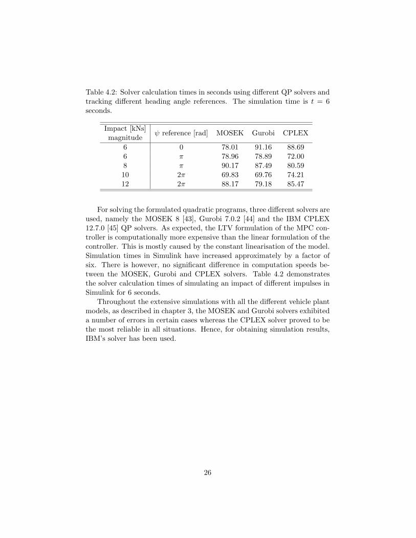
Table 4.2: Solver calculation times in seconds using different QP solvers andtracking different heading angle references. The simulation time is t = 6seconds.

Impact [kNs]magnitude

ψ reference [rad] MOSEK Gurobi CPLEX

6 0 78.01 91.16 88.696 π 78.96 78.89 72.008 π 90.17 87.49 80.5910 2π 69.83 69.76 74.2112 2π 88.17 79.18 85.47

For solving the formulated quadratic programs, three different solvers areused, namely the MOSEK 8 [43], Gurobi 7.0.2 [44] and the IBM CPLEX12.7.0 [45] QP solvers. As expected, the LTV formulation of the MPC con-troller is computationally more expensive than the linear formulation of thecontroller. This is mostly caused by the constant linearisation of the model.Simulation times in Simulink have increased approximately by a factor ofsix. There is however, no significant difference in computation speeds be-tween the MOSEK, Gurobi and CPLEX solvers. Table 4.2 demonstratesthe solver calculation times of simulating an impact of different impulses inSimulink for 6 seconds.

Throughout the extensive simulations with all the different vehicle plantmodels, as described in chapter 3, the MOSEK and Gurobi solvers exhibiteda number of errors in certain cases whereas the CPLEX solver proved to bethe most reliable in all situations. Hence, for obtaining simulation results,IBM’s solver has been used.

26

5 Experiments

Following the implementation of the MPC control algorithms, extensive sim-ulation has been carried out, both in Simulink only and through IPG Car-Maker. For the simulations, as described in chapter 3, two different plantshave been used, gradually adjusting the controller parameters:

A. Four wheel model with a nonlinear Pacejka tire model [17], in Simulink

B. Fourteen DoF model in IPG CarMaker

In all simulation set-ups, a fixed step size of tstep = 0.01 seconds is usedwith an ode3 (Bogacki-Shampine) solver. The vehicle is assumed to travelon a straight road with 100 km/h initial longitudinal velocity at the timeinstance of the impact injection.

5.1 Definition of the main use case

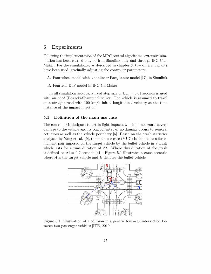
The controller is designed to act in light impacts which do not cause severedamage to the vehicle and its components i.e. no damage occurs to sensors,actuators as well as the vehicle periphery [5]. Based on the crash statisticsanalysed by Yang et. al. [9], the main use case (MUC) is defined as a force-moment pair imposed on the target vehicle by the bullet vehicle in a crashwhich lasts for a time duration of ∆t. Where this duration of the crashis defined as ∆t = 0.2 seconds [41]. Figure 5.1 illustrates a crash-scenariowhere A is the target vehicle and B denotes the bullet vehicle.

Figure 5.1: Illustration of a collision in a generic four-way intersection be-tween two passenger vehicles [ITE, 2010].

27

Figure 5.2: Frequency distribution of impact magnitude by original velocity,presented in [41]

.

Furthermore, because the longitudinal dynamics of the vehicle is notcontrolled directly by the higher layer controller, the impact angle is assumedto be perpendicular to the vehicle’s longitudinal axes i.e. 90 degrees. Thiswill induce a moment of near maximum amplitude on the car and a force inthe lateral direction only. The location of the side impact is assumed to beat the front or rear axles, from either left or right direction, thus yieldingfour sub-cases. Hence the impacts are introduced as a force-moment pair,where the moment (Mimpact) acts on the CoG and the force (Fy,impact) actsin the lateral direction.

The impact magnitude of the MUC is based on data from the GermanIn-Depth Accident Study database [47], analysed by J. Beltran and Y. Song[41]. According to which the impulse magnitude range of 0 - 8 kNs represent61 % of all accidents considered, shown on Figure 5.2. Therefore the impulsemagnitude of the MUC is chosen to be 8 kNs, representing a rather largeimpact. The initial longitudinal velocity of the target vehicle is chosen tobe 100 km/h, representing 78 % of the cases (0 - 100 km/h) studied in thedatabase.

28

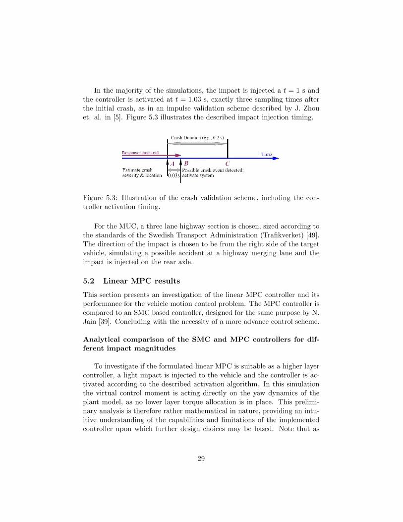
In the majority of the simulations, the impact is injected a t = 1 s andthe controller is activated at t = 1.03 s, exactly three sampling times afterthe initial crash, as in an impulse validation scheme described by J. Zhouet. al. in [5]. Figure 5.3 illustrates the described impact injection timing.

Figure 5.3: Illustration of the crash validation scheme, including the con-troller activation timing.

For the MUC, a three lane highway section is chosen, sized according tothe standards of the Swedish Transport Administration (Trafikverket) [49].The direction of the impact is chosen to be from the right side of the targetvehicle, simulating a possible accident at a highway merging lane and theimpact is injected on the rear axle.

5.2 Linear MPC results

This section presents an investigation of the linear MPC controller and itsperformance for the vehicle motion control problem. The MPC controller iscompared to an SMC based controller, designed for the same purpose by N.Jain [39]. Concluding with the necessity of a more advance control scheme.

Analytical comparison of the SMC and MPC controllers for dif-ferent impact magnitudes

To investigate if the formulated linear MPC is suitable as a higher layercontroller, a light impact is injected to the vehicle and the controller is ac-tivated according to the described activation algorithm. In this simulationthe virtual control moment is acting directly on the yaw dynamics of theplant model, as no lower layer torque allocation is in place. This prelimi-nary analysis is therefore rather mathematical in nature, providing an intu-itive understanding of the capabilities and limitations of the implementedcontroller upon which further design choices may be based. Note that as

29

mentioned before, these initial investigations have been carried out using abicycle model based plant.

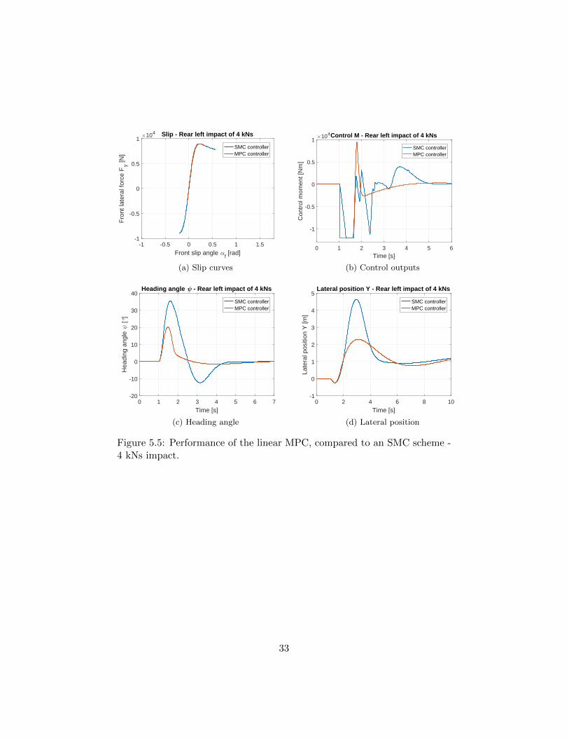
Firstly, responses after an impact of 4 kNs on the rear left axle arestudied, illustrated on Figure 5.5. This imposes a negative lateral force onthe vehicle and a positive moment around the CoG.

The implemented linear MPC controller, based on section 4.2, has thefollowing parameters:

� Ts,MPC = 0.05 s, N = 40, umin = −12 kNm, umax = 12 kNm, ∆umin =−200 kNm/s, ∆umax = 200 kNm/s;

� Q =

7 0 00 2500 00 0 250

, R = 0;

� Constant reference over the horizon: ψref = 0 deg, Yref = 0 m.

Nothe that the horizon N , in all cases, is chosen to be in the range ofN = 1÷ 2 seconds.

Analysing the results, the linear MPC outperforms the SMC with a max-imum heading angle deviation of 20 degrees as opposed to 35.5 degrees, asshown on Figure 5.5c. Also, the vehicle’s heading settles in about 1.5 sec-onds, twice as fast as with the SMC. At the same time, with the formercontroller the vehicle deviates 2.3 meters from its path, exactly half as muchas the maximum deviation with the SMC controller, see Figure 5.5d. Notethat the maximum lateral deviation is not in the negative but in the pos-itive Y direction. Simply due to the heading angle error correction. Themaximum heading angle is fairly close to the prediction model’s operatingpoint (ψ = 0 deg), meaning a low mismatch between the plant and theprediction model, hence the good performance. Furthermore, both the slipcurves and control outputs (Figure 5.5a and 5.5b) show that the MPC con-troller displays a less aggressive behaviour, achieving lover slip angles whilestabilizing the vehicle. This behaviour can be explained by the fact that theMPC is a predictive controller in nature. With the simulated set-up, it op-timizes future vehicle motion 2 seconds ahead in time. Hence the differencein the initial ramp-up of the control signals despite the exact same slew rateconstraints.

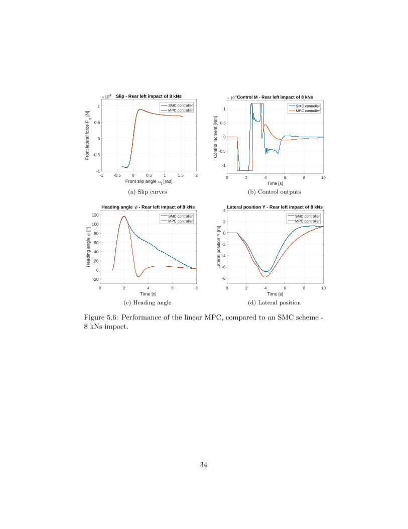
Secondly, an increased impact, the MUC (8 kNs) is simulated with bothcontrollers to further assess the performance. The comparison is demon-strated on Figure 5.6, using the same controller parameters and references.Here the maximum heading angle deviation is around 117 degrees while

30

0 2 4 6 8

time [s]

-50

-40

-30

-20

-10

0

10

20

[m/s

]

Lateral velocity - actual and predicted state

PlantPrediction model

Figure 5.4: The plant’s global lateral velocity (VY ) and the linearized(around ψ = 0) prediction model’s lateral velocity - 8 kNs impact.

approximately 7.8 and 6.8 meters of lateral deviation in the negative Ydirection can be observed with the linear MPC and SMC controllers, re-spectively. As a result of the larger impact, the heading angle’s settlingtimes increase, however the SMC controller seems to minimize the yaw ratetoo quickly allowing a much slower settling of the heading angle. Essentially,the SMC slightly outperforms the MPC. The fact that the vehicle deviatedalmost eight meters from its original path – with MPC control action – callsfor significant improvements. In normal driving scenarios this amount ofdeviation certainly leads to road departure and involves a very high risk ofsecondary collisions.

Surely, one main reason for the poor performance is the rather largemismatch between the linear prediction model’s operating point and theplant’s dynamics at such high heading and slip angles. This model mis-match is demonstrated on Figure 5.4. Between t ≈ 1.2 and t ≈ 2.8 secondsthe vehicle’s heading angle is in a region above 20 degrees. Consequently,the global lateral velocity calculated by the MPC’s prediction model devi-ates substantially from the plants global lateral velocity. When minimizingthe objective function with respect to the lateral deviation, this error isaccumulated (integrated) resulting in incorrect reference tracking along theprediction horizon thus poor control performance.

Another main reason for the dissatisfactory control performance is dueto the prediction model formulation. A constant lateral velocity is assumedin the model which when the vehicle turns more than ± 90 degrees points inthe opposite direction. This means that the linear bicycle prediction modelcan not settle at any different ”optimal” heading angle than zero. This raises

31

the question whether zero degrees is the optimal heading angle to track inthe MUC.

Therefore, in order to minimize model mismatch when optimizing futurevehicle motion, and allow settling at heading angles different than zero, amore elaborate prediction model has to be used. Furthermore, to avoid thecomputational burden of nonlinear MPC [34], choosing a linear time varyingMPC is a well motivated decision.

32

-1 -0.5 0 0.5 1 1.5

Front slip angle f [rad]

-1

-0.5

0

0.5

1

Fro

nt la

tera

l for

ce F

y [N]

104 Slip - Rear left impact of 4 kNs

SMC controllerMPC controller

(a) Slip curves

0 1 2 3 4 5 6Time [s]

-1

-0.5

0

0.5

1

Con

trol

mom

ent [

Nm

]

104Control M - Rear left impact of 4 kNs

SMC controllerMPC controller

(b) Control outputs

0 1 2 3 4 5 6 7

Time [s]

-20

-10

0

10

20

30

40

Hea

ding

ang

le

[°]

Heading angle - Rear left impact of 4 kNs

SMC controllerMPC controller

(c) Heading angle

0 2 4 6 8 10

Time [s]

-1

0

1

2

3

4

5

Late

ral p

ositi

on Y

[m]

Lateral position Y - Rear left impact of 4 kNs

SMC controllerMPC controller

(d) Lateral position

Figure 5.5: Performance of the linear MPC, compared to an SMC scheme -4 kNs impact.

33

-1 -0.5 0 0.5 1 1.5 2

Front slip angle f [rad]

-1

-0.5

0

0.5

1

Fro

nt la

tera

l for

ce F

y [N]

104 Slip - Rear left impact of 8 kNs

SMC controllerMPC controller

(a) Slip curves

0 2 4 6 8 10

Time [s]

-1

-0.5

0

0.5

1

Con

trol

mom

ent [

Nm

]

104Control M - Rear left impact of 8 kNs

SMC controllerMPC controller

(b) Control outputs

0 2 4 6 8

Time [s]

-20

0

20

40

60

80

100

120

Hea

ding

ang

le

[°]

Heading angle - Rear left impact of 8 kNs

SMC controllerMPC controller

(c) Heading angle

0 2 4 6 8 10

Time [s]

-8

-6

-4

-2

0

2

4

Late

ral p

ositi

on Y

[m]

Lateral position Y - Rear left impact of 8 kNs

SMC controllerMPC controller

(d) Lateral position

Figure 5.6: Performance of the linear MPC, compared to an SMC scheme -8 kNs impact.

34

5.3 LTV-MPC results

To improve the control performance a more advanced concept, LTV-MPCis implemented for the same vehicle motion control problem. The main aimof using LTV-MPC is to effectively control vehicle motion in high slip anglesituations, when the vehicle may spin half a rotation or even more. Thusthis section presents the controller’s capability of making the vehicle settle atheading angles of multiples of π, other then zero. The controller is primarilytested in the MUC with the two track plant model in simulation.

5.3.1 Performance comparison

The implemented LTV-MPC is tested in the MUC with the impact actingon the rear left axle. As before, at t = 1 an impulse of 8 kNs is injected fora duration of 0.2 seconds. The controller has the following parameters:

� Ts,MPC = 0.2 s, N = 6, umin = −12 kNm, umax = 12 kNm, ∆umin =−200 kNm/s, ∆umax = 200 kNm/s;

� Q =

2500 0 00 250 00 0 7

, R = 0;

� Constant reference over the horizon: ψref = 0 deg, Yref = 0 m.

Since the heading angle deviation has crossed 90 degrees with the linearMPC, seen on 5.6c, tracking ψref = π heading angle reference is added tothe comparison. Although here a slightly modified weight matrix Q′ is used,

Q′ =

2450 0 00 20 00 0 3

Figure 5.8 demonstrates the performance of the LTV-MPC tracking both

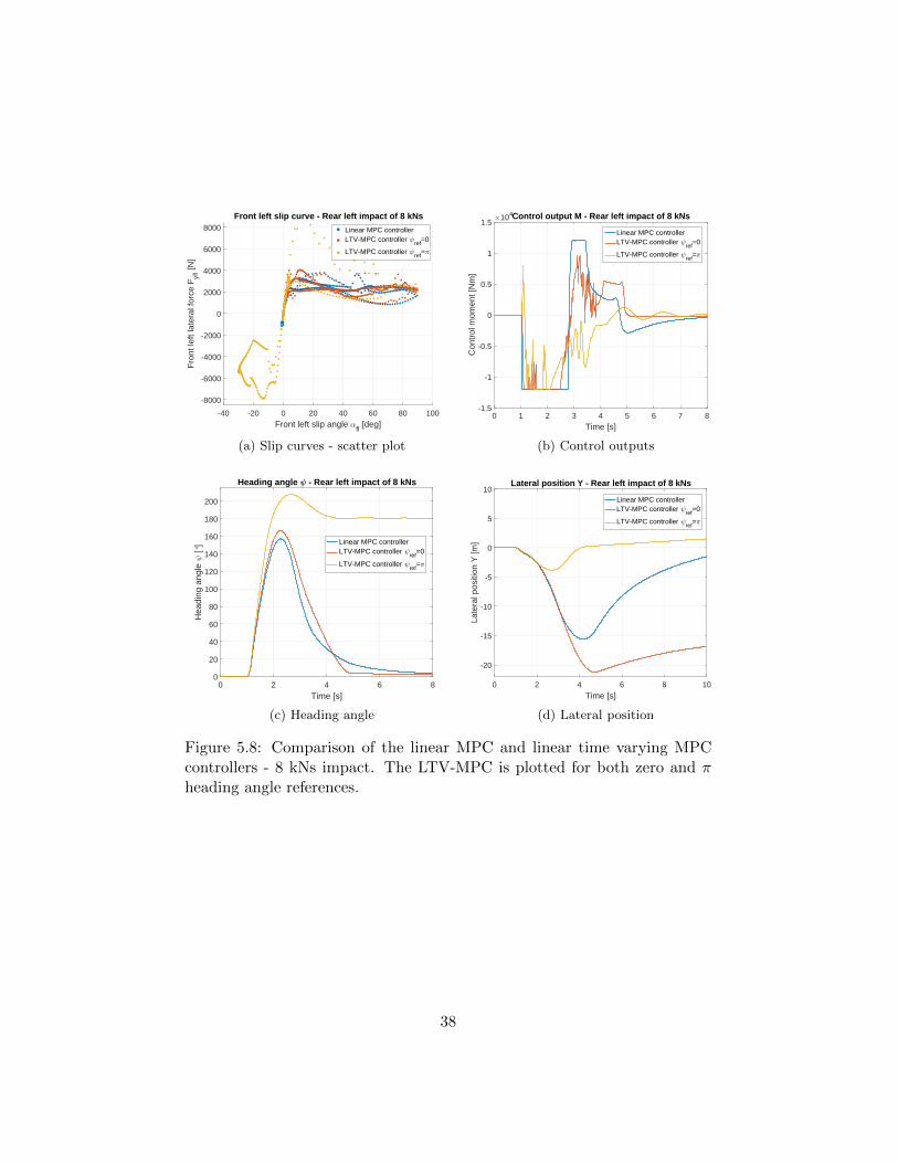
ψref = 0 and ψref = π references and the linear MPC controller, still trackingzero heading angle.

Results suggest very interesting behaviours. First of all, when trackingzero heading angle reference – contrary to expectations – the LTV-MPCseems to perform worse than the linear MPC. The question why this ishappening can be answered when analysing the system states with the LTV-MPC tracking π heading angle i.e. allowing half a rotation. In simpleterms, for the injected impact settling at 180 degrees gives substantially

35

less lateral deviation from the original path, thus this heading angle can becalled optimal for the case.

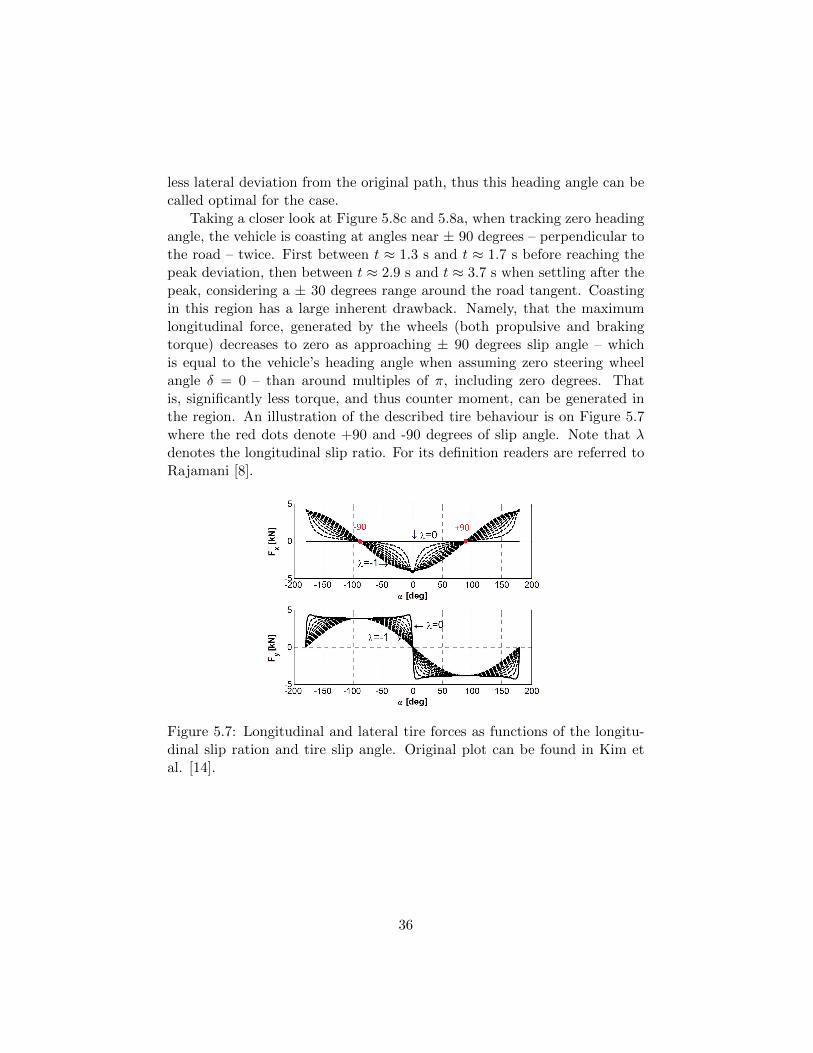
Taking a closer look at Figure 5.8c and 5.8a, when tracking zero headingangle, the vehicle is coasting at angles near ± 90 degrees – perpendicular tothe road – twice. First between t ≈ 1.3 s and t ≈ 1.7 s before reaching thepeak deviation, then between t ≈ 2.9 s and t ≈ 3.7 s when settling after thepeak, considering a ± 30 degrees range around the road tangent. Coastingin this region has a large inherent drawback. Namely, that the maximumlongitudinal force, generated by the wheels (both propulsive and brakingtorque) decreases to zero as approaching ± 90 degrees slip angle – whichis equal to the vehicle’s heading angle when assuming zero steering wheelangle δ = 0 – than around multiples of π, including zero degrees. Thatis, significantly less torque, and thus counter moment, can be generated inthe region. An illustration of the described tire behaviour is on Figure 5.7where the red dots denote +90 and -90 degrees of slip angle. Note that λdenotes the longitudinal slip ratio. For its definition readers are referred toRajamani [8].

Figure 5.7: Longitudinal and lateral tire forces as functions of the longitu-dinal slip ration and tire slip angle. Original plot can be found in Kim etal. [14].

36

Table 5.1: Performance comparison of the linear MPC and LTV-MPCcontrollers. With the LTV-MPC, two different reference heading angle istracked.

Controller ψmax [deg] Ymax [m] tsettling [s]

Linear MPC 157 -21.22 4.6LTV-MPC, ψref = 0 166.3 -15.64 3.6LTV-MPC, ψref = ψ 207.8 -3.83 3

Table 5.1 summarizes the three compared controllers’ performance. Ithas been shown that the LTV-MPC controller, tracking ψref = π, reduces thelateral deviation to a maximum of 3.8 meters in the global frame’s negativedirection. Meaning a departure from the original lane and violating theadjacent lane, reducing the chance of a secondary collisions. This allows todraw the conclusion that tracking the optimal final heading angle referenceis really crucial to achieve sufficiently good controller performance. It hasalso been demonstrated that extending the MPC’s prediction model wasnecessary to allow settling at different heading angles. With the newlygained intuitions and understanding, simulations with a high fidelity vehicledynamics model is a natural extension.

37

-40 -20 0 20 40 60 80 100Front left slip angle

fl [deg]

-8000

-6000

-4000

-2000

0

2000

4000

6000

8000

Fro

nt le

ft la

tera

l for

ce F

yfl [N

]

Front left slip curve - Rear left impact of 8 kNs

Linear MPC controllerLTV-MPC controller

ref=0

LTV-MPC controller ref

=

(a) Slip curves - scatter plot

0 1 2 3 4 5 6 7 8Time [s]

-1.5

-1

-0.5

0

0.5

1

1.5

Con

trol

mom

ent [

Nm

]

104Control output M - Rear left impact of 8 kNs

Linear MPC controllerLTV-MPC controller

ref=0

LTV-MPC controller ref

=

(b) Control outputs

0 2 4 6 8Time [s]

0

20

40

60

80

100

120

140

160

180

200

Hea

ding

ang

le

[°]

Heading angle - Rear left impact of 8 kNs

Linear MPC controllerLTV-MPC controller

ref=0

LTV-MPC controller ref

=

(c) Heading angle

0 2 4 6 8 10Time [s]

-20

-15

-10

-5

0

5

10

Late

ral p

ositi

on Y

[m]

Lateral position Y - Rear left impact of 8 kNs

Linear MPC controllerLTV-MPC controller

ref=0

LTV-MPC controller ref

=

(d) Lateral position

Figure 5.8: Comparison of the linear MPC and linear time varying MPCcontrollers - 8 kNs impact. The LTV-MPC is plotted for both zero and πheading angle references.

38

5.3.2 Simulations with IPG CarMaker

A generic sedan is defined in IPG CarMaker based on the Saab 9-3 compactexecutive car, using vehicle parameters of [48]. The control action is acti-vated after the injected impact, just as before and an additional deactivationalgorithm is deployed handing the control back to the driver model if theyaw rate is below a threshold of 2 deg/s for 50 iterations (i.e. half a second).

During the process of tuning the controllers, results of two different out-put maps, hA and hB have been compared. Where output map hA is definedby equation (3.21) and hB is,

hB =

[0 0 1 0 0 00 0 0 0 1 0

](5.1)

By changing the output map from hA to hB the yaw rate ψ is excludedfrom the minimization. This should intuitively not increase the control per-formance significantly. Extensive simulation results, using a prediction hori-zon of N = 5÷ 6, allow however to draw the following general conclusions:in most cases, exclusion of the yaw rate from the performance index allows amuch quicker settling of the heading angle. Maximum lateral deviations areonly slightly affected. Nevertheless, controller performance mainly dependson the injected impact’s magnitude and the performance difference due tochoosing one output map over the other is insignificant.

With the vehicle’s plant model defined in IPG CarMaker, the controllerapplied in the MUC has the following parameters:

� Ts,MPC = 0.2 s, N = 5, umin = −12 kNm, umax = 12 kNm, ∆umin =−200 kNm/s, ∆umax = 200 kNm/s;

� Q =

2550 0 00 20 00 0 3

, R = 0;

� Constant reference over the horizon: ψref = 180 deg, Yref = 0 m.

The performance of the controller is demonstrated on Figure 5.9. Asseen using the two track plant model, the heading angle trajectory displays aconsiderable overshoot before settling at π. This results in a lateral deviationfrom the original path in both directions, as shown on Figure 5.9d. Afterdeparture from the original lane as a direct consequence of the impact, thevehicle deviates towards the opposite direction while correcting the heading

39

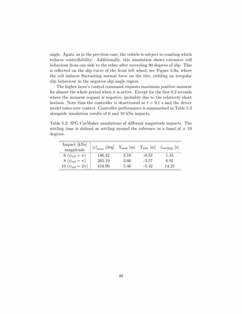
angle. Again, as in the previous case, the vehicle is subject to coasting whichreduces controllability. Additionally, this simulation shows extensive rollbehaviour from one side to the other after exceeding 90 degrees of slip. Thisis reflected on the slip curve of the front left wheel, see Figure 5.9a, wherethe roll induces fluctuating normal force on the tire, yielding an irregularslip behaviour in the negative slip angle region.

The higher layer’s control command requests maximum positive momentfor almost the whole period when it is active. Except for the first 0.2 secondswhere the moment request is negative, probably due to the relatively shorthorizon. Note that the controller is deactivated at t = 9.1 s and the drivermodel takes over control. Controller performance is summarised in Table 5.2alongside simulation results of 6 and 10 kNs impacts.

Table 5.2: IPG CarMaker simulations of different magnitude impacts. Thesettling time is defined as settling around the reference in a band of ± 10degrees.

Impact [kNs]magnitude

|ψ|max [deg] Ymax [m] Ymin [m] tsettling [s]

6 (ψref = π) 186.42 3.10 -0.52 1.458 (ψref = π) 265.19 3.66 -3.57 6.91

10 (ψref = 2π) 416.90 5.46 -5.42 14.25

40

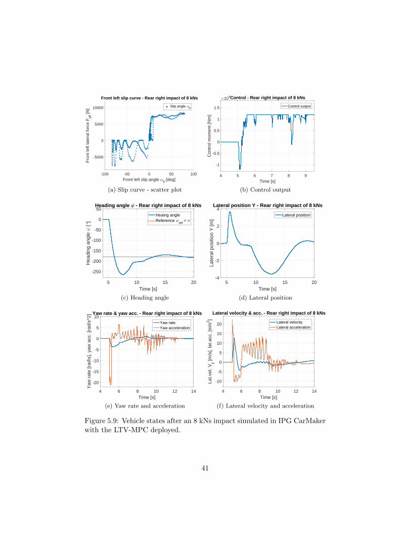
-100 -50 0 50 100Front left slip angle

fl [deg]

-5000

0

5000

10000

Fro

nt le

ft la

tera

l for

ce F

yfl [N

]

Front left slip curve - Rear right impact of 8 kNs

Slip angle fl

(a) Slip curve - scatter plot

4 5 6 7 8 9Time [s]

-1

-0.5

0

0.5

1

1.5

Con

trol

mom

ent [

Nm

]

104Control - Rear right impact of 8 kNs

Control output

(b) Control output

5 10 15 20

Time [s]

-250

-200

-150

-100

-50

0

50

Hea

ding

ang

le

[°]

Heading angle - Rear right impact of 8 kNs

Heaing angleReference

ref =

(c) Heading angle

5 10 15 20

Time [s]

-4

-2

0

2

4La

tera

l pos

ition

Y [m

]Lateral position Y - Rear right impact of 8 kNs

Lateral position

(d) Lateral position

4 6 8 10 12 14Time [s]

-20

-15

-10

-5

0

5

10

Yaw

rat

e [r

ad\s

], ya

w a

cc. [

rad/

s^2]

Yaw rate & yaw acc. - Rear right impact of 8 kNs

Yaw rateYaw acceleration

(e) Yaw rate and acceleration

4 6 8 10 12 14Time [s]

-10

-5

0

5

10

15

20

Lat.v

el. V

y [m/s

], la

t.acc

. [m

/s2 ]

Lateral velocity & acc. - Rear right impact of 8 kNs

Lateral velocityLateral acceleration

(f) Lateral velocity and acceleration

Figure 5.9: Vehicle states after an 8 kNs impact simulated in IPG CarMakerwith the LTV-MPC deployed.

41

5 6 7 8 9 10 11Time [s]

-2000

-1000

0

1000

2000W

heel

torq

ue r

eque

sts

[Nm

]Wheel torque requests - Rear right impact of 8 kNs

FLFRRLRR

(a) Torque requests

4 6 8 10 12 14

Time [s]

-1

-0.5

0

0.5

1

Long

itudi

nal s

lip r

atio

s

Longitudinal slip ratios - Rear right impact of 8 kNs

FLFRRLRR

(b) Longitudinal slip ratios

Figure 5.10: Longitudinal slip ratios and torque requests on the wheels(motors) after an 8 kNs impact simulated in IPG CarMaker with the LTV-MPC deployed.

It is worth taking a look at the lower layer’s output. Figure 5.10a dis-plays the torque requests on the wheels whereas Figure 5.10b shows thelongitudinal slip ratios λ at each wheel throughout the MUC. At first sightthe requested slips seem to be rather fluctuating and this apparently resultsin a similar trend of the slip ratios. However, since the MUC is an emergencyscenario, overloading the actuators and saturating the tires is not necessarilya major concern, given that the safety limits are not exceeded.

To better illustrate what is really happening with the vehicle post-crash,Figure 5.11 shows the vehicle’s trajectories subject to a 6 and 8 kNs impact,demonstrating the scenarios with and without controller action.

42

100 120 140 160 180 200 220 240 260Longitudinal distance [m]

-6

-4

-2

0

2

4

6

Late

ral d

evia

tion

[m]

Vehicle trajectory with and without controller action, rear right impact of 6kNs

Controlled - headingControlled - trajectoryUncontrolled - headingUncontrolled - trajectory

(a) Vehicle trajectory after a 6 kNs impact

100 120 140 160 180 200 220 240 260Longitudinal distance [m]

-6

-4

-2

0

2

4

6

Late

ral d

evia

tion

[m]

Vehicle trajectory with and without controller action, rear right impact of 8kNsControlled - headingControlled - trajectoryUncontrolled - headingUncontrolled - trajectory

(b) Vehicle trajectory after an 8 kNs impact

Figure 5.11: Vehicle trajectories after a 6 and 8 kNs impact simulated inIPG CarMaker with the LTV-MPC deployed. The open loop trajectoriesare included as a reference.

In this section it has been shown that a vehicle in the MUC deviatesaround 3.6 meters in the direction of the impact and then deviates thesame distance in the opposite direction due to overcompensation and thedecreased yaw rate. Theoretically, if the vehicle is travelling in any of thelanes of a three lane highway, when the impact occurs, the controller issuitable to save the vehicle from crashing into the left or right road bar-riers. This allows to conclude that actuation exclusively through brakingand propulsive torques (i.e. torque vectoring) and using LTV-MPC in thehigher control layer, is a suitable method to mitigate secondary collisions.It is however important to note that active steering could potentially fur-ther decrease the lateral deviation and eliminate additional deviation whensettling after an overshoot of the heading angle.

43

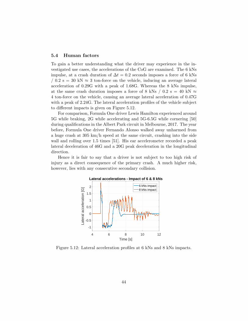
5.4 Human factors

To gain a better understanding what the driver may experience in the in-vestigated use cases, the accelerations of the CoG are examined. The 6 kNsimpulse, at a crash duration of ∆t = 0.2 seconds imposes a force of 6 kNs/ 0.2 s = 30 kN ≈ 3 ton-force on the vehicle, inducing an average lateralacceleration of 0.29G with a peak of 1.68G. Whereas the 8 kNs impulse,at the same crash duration imposes a force of 8 kNs / 0.2 s = 40 kN ≈4 ton-force on the vehicle, causing an average lateral acceleration of 0.47Gwith a peak of 2.24G. The lateral acceleration profiles of the vehicle subjectto different impacts is given on Figure 5.12.

For comparison, Formula One driver Lewis Hamilton experienced around5G while braking, 2G while accelerating and 5G-6.5G while cornering [50]during qualifications in the Albert Park circuit in Melbourne, 2017. The yearbefore, Formula One driver Fernando Alonso walked away unharmed froma huge crash at 305 km/h speed at the same circuit, crashing into the sidewall and rolling over 1.5 times [51]. His ear accelerometer recorded a peaklateral deceleration of 46G and a 20G peak deceleration in the longitudinaldirection.

Hence it is fair to say that a driver is not subject to too high risk ofinjury as a direct consequence of the primary crash. A much higher risk,however, lies with any consecutive secondary collision.

4 6 8 10 12

Time [s]

-1

-0.5

0

0.5

1

1.5

2

Late

ral a

ccel

erat

ion

[G]

Lateral accelerations - Impact of 6 & 8 kNs

6 kNs impact8 kNs impact

Figure 5.12: Lateral acceleration profiles at 6 kNs and 8 kNs impacts.

44

6 Conclusion and further work

Throughout this thesis the design steps of an active safety system have beendescribed, proposing a vehicle motion control algorithm for post-crash sce-narios, aiming to minimize lateral deviation from the original lane whileachieving a safe heading angle. For the control problem, a model basedcontrol algorithm is chosen, namely model predictive control.. Therefore,careful modelling of the vehicle dynamics as plant and as prediction modelhas been carried out. Then a simple time invariant linear MPC and a morecomplex linear time varying MPC is designed. Parallel to the design pro-cess extensive simulations have been run to assist the main design decisionsarguing the necessity of the more sophisticated controller. Results of theLTV-MPC formulation show that a vehicle subject to an initial crash de-fined in the main use case can be saved from secondary collision with theroad boundaries on a standard three lane highway, violating only the adja-cent lanes while recovering to a stable state. Thereby, the conclusion is thatMPC indeed is a suitable higher layer controller in a hierarchical controlarchitecture, for the described post-crash vehicle motion control problem.

In the following sections, possible extensions to the overall control archi-tecture and to the MPC formulation are discussed.

6.1 Extensions of the controller architecture

Considering the active safety function as a whole, several subfunctions areleft unexplored. First of all a suitable online system identification scheme re-mains to be elaborated. Such a system would enable to account for changingvehicle dynamics properties, detect actuator and sensor damage or failuresand other faults. Second, the controller’s activation and deactivation al-gorithm shall be studied in more detail. A crucial point here is the exacttiming of these algorithms. In a crash scenario the activation algorithm hasto act as soon as possible, without any misdetection. And the controllerdeactivation has to ensure safe hand-back of control to the driver. Analy-sis on human factors is key, as to determine this exact timing. Perhaps alearning algorithm could be utilised as such, to adapt to different driver re-action profiles. Another obvious further improvement of the control systemis to introduce a supervisory controller scheme, regulating the longitudinaldynamics of the vehicle in post-crash scenarios. Just as the human instinctimplies, this controller should reduce the vehicle’s longitudinal velocity withrespect to the global coordinate frame, bringing the vehicle to a safe stop.Furthermore, utilizing the perception of vehicles’ environment, commonly

45

available in today’s cars, fusing the data of multiple sensors e.g., camerasand radars, improved higher level decision making could be achieved. Itwould also allow more elaborate reference generation. For example follow-ing a nonlinear, curved path as a reference while the controller is active.The vehicle motion control algorithm, described in this thesis assumes animpact detection scheme in place. Determining the magnitude, directionand exact location of the impact is required for the system to work. Sucha scheme could be assisted by the vehicle’s perception, even in a predictivemanner. Introducing another actuator to the already over-actuated system– namely active steering – could drastically change the control performance.A frequent outcome of the method in this thesis is the fact that when the ve-hicle’s yaw rate gets reduced to the vicinity of zero, actuation only throughthe four wheels cannot efficiently reduce heading angle errors with respectto the reference. Adding active steering would of course impose additionalcomplexity to the control system, trading off computational effort. On topof that, a steer-by-wire system would be necessary in the vehicle with anappropriate human-machine interface.

6.2 Extensions of the MPC formulation

Finding the correct penalty weights of the objective function proved to bea long and empirical process due to frequent infeasibility of the optimiza-tion. Therefore finding out which constraints are violated and adding a slackvariable to these constraints would be a logical and necessary extension. Bysoftening these constraints, feasibility may be assured with an even longerprediction horizon, allowing to optimize future vehicle motion further aheadin time. Additionally, investigating the applicability of adaptive weight ma-trices might give significant increase of controller performance. Nevertheless,the problem may be infeasible independently of the penalty weights. Re-vised formulation of the MPC could also be an interesting extension. Forexample, defining the longitudinal and lateral forces – perhaps even thelongitudinal slip values – as control outputs and including the tire forcelimitations directly as constraints. Furthermore, since robustness is an es-sential aspect of active safety systems, exploring robust and nonlinear MPCtechniques is another possible extension of the project. Improving compu-tational efficiency, further investigation of the available QP solvers could bedone, considering both specific software and hardware solutions, allowingreal-time implementability.

46

References

[1] European Commission - Press Release Database, 2016 roadsafety statistics: What is behind the figures?, [Online]. Available:http://europa.eu/rapid/press-release MEMO-17-675 en.htm, [Ac-cessed: 2017-07-20]

[2] D. Yang, B. Jacobson, and M. Lidberg, Benefit prediction of passengercar post impact stability control based on accident statistics and vehi-cle dynamics simulations, Proceedings of 21st IAVSD Symposium onDynamics of Vehicles on Roads and Tracks, 2009.

[3] S. I. Sakai, H. Sado, Y. Hori, Motion Control in an Electric Vehiclewith Four Independently Driven In-Wheel Motors, IEEE/ASME Trans-actions on Mechatronics, vol. 4, NO. 1, March, 1999.

[4] K. Yoshimoto, H. Tanaka, S.Kawakami, Proposal of Driver AssistanceSystem for Recovering Vehicle Stability from Unstable States by Au-tomatic Steering, Dept. of Mechano-Informatics, University of Tokyo,1999.

[5] J. Zhou, J. Lu, H. Peng, Vehicle Stabilization in Response to ExogenousImpulsive Disturbances to the Vehicle Body, 2009 American ControlConference, Hyatt Regency Riverfront, St. Louis, MO, USA, June 10-12, 2009.

[6] R. Wang, H. R. Karimi, N. Chen, G. Yin, J. Wang, Motion Control ofFour-Wheel Independently Actuated Electric Ground Vehicles consid-ering Tire Force Saturation, Hindawi Publishing Corporation, Mathe-matical Problems in Engineering, Article ID 819302, 8 pages, Volume2013.

[7] K. Sawase, Y. Sano, Application of active Yaw control to vehicle dynam-ics by utilizing driving/braking force, New Technologies & New Cars,JSAE Review 20 289-295, 1999.

[8] R. Rajamani, Vehicle dynamics and control, Mechanical EngineeringSeries, Second Edition, Springer, 2012.

[9] D. Yang, Vehicle Dynamics Control after Impacts in Multiple-Event Ac-cidents, Thesis for the Degree of Doctor of Philosophy in Machine andVehicle Systems, Department of Applied Mechanics, Chalmers Univer-sity of Technology, Goteborg, Sweden, 2013.

47

[10] A. Haussler, R. Schaffler, A. Georgi, S. Stabrey, Networking of airbagand ESP for prevention of further collisions., ATZ - Automobiltechnis-che Zeitschrift, vol. 114, pp. 22-26, 2012.

[11] D. Wanner, Controlling over-actuated road vehicles during failure condi-tions, Doctoral Thesis, KTH Royal Institute of Technology, Stockholm,Sweden, 2015.

[12] J. Zhou, H. Peng and J. Lu, Collision model for vehicle motion predic-tion after light impacts, Vehicle System Dynamics, Vol. 46, Supplement,2008.

[13] B.J. Kim, H. Peng, Vehicle Stability Control of Heading Angle and Lat-eral Deviation to Mitigate Secondary Collisions, University of Michigan,11th International Symposium on Advanced Vehicle Control (AVEC),Seoul, South Korea, 2012.

[14] B. Kim, Huei Peng, Optimal Vehicle Motion Control to Mitigate Sec-ondary Crashes After an Initial Impacts, 2014 ASME Dynamic Systemsand Control Conference, San Antonio, TX, Oct. 22-24, 2014. Winnerof the 2014 DSCC Best Student Paper Award.

[15] V. Turri, A. Carvalho, H. E. Tseng, K. H. Johansson, F. Borelli, Lin-ear Model Predictive Control for Lane Keeping and Obstacle Avoidanceon Low Curvature Roads, Proceedings of the 16th International IEEEAnnual Conference on Intelligent Transportation Systems (ITSC 2013),The Hague, The Netherlands, October 6-9, 2013.

[16] P. Falcone, F. Borelli, H. E. Tseng, J. Asgari, D. Hrovat, Low Complex-ity MPC Schemes for Integrated Vehicle Dynamics Control Problems,Vol. 402Automotive Model Predictive Control, pp. 211-230, 2010.

[17] H. B. Pacejka, Tire and Vehicle Dynamics, Second edition, SAE Inter-national, 2015.

[18] NHTSA: Traffic Safety Facts 2006. NHTSA Report DOT HS 810 818(2008).

[19] A. Eigen, W. Najm, Problem definition for pre-crash sensing advancedrestraints, DOT HS 811 114, 2009.

[20] S. A. Ferguson, The effectiveness of electronic stability control in reduc-ing real-world crashes: a literature review, Traffic Injury Prevention,vol. 8, pp. 329-338, 2007.

48

[21] A. Erke, Effects of electronic stability control on accidents: A reviewof empirical evidence, Accident Analysis and Prevention, vol. 40, no. 1,pp.167-173, 2008.

[22] B. Fildes, J. C. Lane, J. Lenard, A. Vlcan, Passenger cars and occupantinjury: side impact crashes, 1994.

[23] IEA/OECD, World Energy Outlook 2012, International Energy Agencyand Organisation for Economic Co-operation and Development, Tech.Rep., 2012.

[24] J. Bahouth, K. Digges, ”Characteristics of Multiple Impact CrashesThat Produce Serious Injuries,” in Proceedings of the 19th InternationalTechnical Conference on the Enhanced Safety of Vehicles, WashingtonDC, USA, 2005.

[25] U. Sander, K. Mroz, O. Bostrom, R. Fredriksson, ”The effect of pre-pretensioning in multiple impact crashes,” in 21st International Tech-nical Conference on the Enhanced Safety of Vehicles (ESV), 2009.

[26] A. Togawa, D. Murakami, H. Saeki, C. Pal, T. Okabe, ”An Insightinto Multiple Impact Crash Statistics to Search for Future Directionsof Counter-Approaches,” in 22th International Technical Conference onthe Enhanced Safety of Vehicles (ESV), 2011.

[27] J. Lenard and R. Frampton, Two-Impact Crashes-Implications for Oc-cupant Protection Technologies, in Proceedings of 18th InternationalTechnical Conference on the Enhanced Safety of Vehicles, Nagoya,Japan, 2003.

[28] C. Song, F. Xiao, S. Song, S. Li, J. Li, Stability control of 4WD electricvehicle with in-wheel motors based on sliding mode control, Sixth inter-national conference on intelligent control and information processing,2015.

[29] B.J. Kim, H. Peng, Collision Strength Estimation and Preemptive Steer-ing Control for Post-Impact Vehicle Motion Control, In 12th Interna-tional Symposium on Advanced Vehicle Control, September, 2014.

[30] F. Gustafsson, Slip-based tire-road friction estimation, Automatica 33.6(1997): 1087-1099.

49

[31] A. Albinsson, Tire Force Estimation Utilizing Wheel Torque Measure-ments and Validation in Simulations and Experiments, 12th Interna-tional Symposium on Advanced Vehicle Control (AVEC’14), Tokyo,Japan, 2014.

[32] Dimos Dimarogonas, EL2425 - Hybrid and Embedded Control Systems,Reading Material, School of Electrical Engineering, KTH Royal Insti-tute of Technology, Stockholm, Sweden, 2016.

[33] F. Borelli, A. Bemporad, M. Morari, Predictive Control for Linear andHybrid Systems, October 19, 2015.

[34] P. Falcone, F. Borelli, J. Asgari, H. E. Tseng, D. Hrovat, Predictiveactive steering control for autonomous vehicle systems, IEEE Transac-tions on Control System Technology, vol. 15, no. 3, May, 2007.

[35] P. Falcone, M. Tufo, F. Borelli, J. Asgari, H. E. Tseng, A Linear TimeVarying Model Predictive Controller Approach to the Integrated VehicleDynamics Control Problem in Autonomous Systems, IEEE, 2007.

[36] P. Falcone, F. Borelli, H. E. Tseng, J. Asgari, D. Hrovat, Linear time-varying model predictive control and its application to active steeringsystems: Stability analysis and experimental validation, InternationalJournal of Robust Nonlinear Control, 2008., 18:862-875

[37] P.Falcone, F. Borelli, H. E. Tseng, J. Asgari, D. Hrovat, Linear time-varying model predictive control and its application to active steer-ing systems: Stability analysis and experimental validation, Interna-tional Journal of Robust and Nonlinear Control, Published online 18July 2007 in Wiley InterScience (www.interscience.wiley.com). DOI:10.1002/rnc.1245

[38] C. Chatzikomis, A. Sorniotti, P. Gruber, M. Bastin, et al., Torque-Vectoring Control for an Autonomous and Driverless Electric RacingVehicle with Multiple Motors, SAE Int. J. Veh. Dyn., Stab., and NVH1(2):338-351, 2017, doi:10.4271/2017-01-1597.

[39] N. Jain, Robust post impact vehicle motion control using torque vec-toring, MSc. Thesis, School of Aeronautical and Vehicle Engineering,KTH Royal Institute of Technology, Stockholm, Sweden, 2017.

[40] R. Samefors, K. J. Hagelin, Vehicle Motion Priority, Motion Analysisof Deceleration While Cornering, MSc. Thesis, Department of Applied

50

Mechanics, Division of Vehicle Engineering and Autonomous Systems,Chalmers University of Technology, Goteborg, Sweden, 2016.

[41] J. Beltran and Y. Song, Methods for verification of post impact controlincluding driver interaction Master’s Thesis 2011:11, ISSN 1652-8557,Chalmers University of Technology, 2011.

[42] IPG Automotive, CarMaker model environment, [Online]. Available:https://ipg-automotive.com/, [Accessed: 2017-07-06]

[43] MOSEK ApS, MOSEK QP solver, [Online]. Available:https://mosek.com/, [Accessed: 2017-06-12]

[44] Gurobi, Gurobi Optimizer 7.0, [Online]. Available:http://www.gurobi.com, [Accessed: 2017-06-12]

[45] IBM, IBM ILOG CPLEX Optimizer Studio, [Online]. Available:https://www-01.ibm.com/software/commerce/optimization/cplex-optimizer/, [Accessed: 2017-06-12]

[46] Johan Lofberg, YALMIP, [Online]. Available:https://yalmip.github.io/, [Accessed: 2017-06-12]

[47] VUFO GmbH, Unfallforschung - GIDAS, [Online]. Available:http://www.vufo.de/forschung-und-entwicklung/gidas/, [Accessed:2017-04-18]

[48] saabmedia.net, Model specifications, [Online]. Available:https://web.archive.org/web/20070929015213/http://www.saabmedia.net/models/9-3/pressinfo/2008-SS-SC/specifications/index.html,[Accessed: 2017-06-25]

[49] Vagverket, Svenska Kommunforbundet, Vagar och gators utformning,ISSN:1401-9612, 2004.

[50] formula1.com, Analysing 2017’s massive rises in G-Force, [Online].Available: https://www.formula1.com/en/latest/features/2017/3/f1-video-2017-vs-2016-g-force-comparison.html, [Accessed: 2017-07-19]

[51] fia.com, F1 - SAFETY MEASURES, [Online]. Available:http://www.fia.com/news/f1-safety-measures, [Accessed:2017-07-19]

TRITA EE 2017:015ISSN 1653-5146

www.kth.se