1/11 طراحی و آموزش شبکه های عصبی slide from dr. m. pomplun

1/11

های شبکه آموزش و طراحیعصبی

Slide from Dr. M. Pomplun

2

In supervised learning:

• We train an ANN with a set of vector pairs, so-called exemplars.

• Each pair (x, y) consists of an input vector x and a corresponding

output vector y.

• Whenever the network receives input x, we would like it to provide

output y.

• The exemplars thus describe the function that we want to “teach”

our network.

• Besides learning the exemplars, we would like our network to

generalize, that is, give plausible output for inputs that the network

had not been trained with.

3

Classification

Neural networks have been used success fully in a large number of practical classificationtasks, such as the following:•Recognizing printed or handwritten characters•Classifying loan applications into credit-worthy and non-credit-worthy groups•Analyzing sonar and radar data to determine the nature of the source of a signal

4

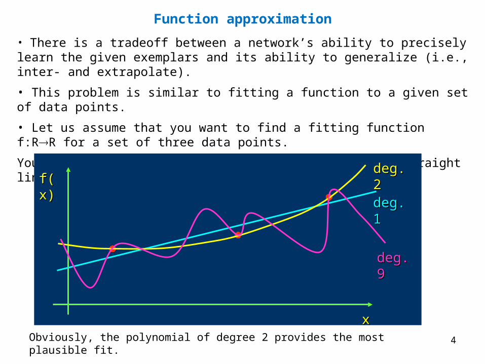
• There is a tradeoff between a network’s ability to precisely learn the given exemplars and its ability to generalize (i.e., inter- and extrapolate).

• This problem is similar to fitting a function to a given set of data points.

• Let us assume that you want to find a fitting function f:RR for a set of three data points.

You try to do this with polynomials of degree one (a straight line), two, and nine.

f(x)f(x)

xx

deg. 1deg. 1

deg. 2deg. 2

deg. 9deg. 9

Obviously, the polynomial of degree 2 provides the most plausible fit.

Function approximation

5

The same principle applies to ANNs:

• If an ANN has too few neurons, it may not have enough degrees of freedom to precisely approximate the desired function.

• If an ANN has too many neurons, it will learn the exemplars perfectly, but its additional degrees of freedom may cause it to show implausible behavior for untrained inputs; it then presents poor ability of generalization.

• Unfortunately, there are no known equations that could tell you the optimal size of your network for a given application; there are only heuristics.

6

Evaluation of networks

Basic idea: define error function and measure error for untrained data (testing set)

• Typical:

where d is the desired output, and o is the actual output.

Root Mean square error:

i

ii od 2)(E

N

odi

ii

2)(E

7

Data Representation

All networks process one of two types of signal components: analog (continuously variable) signals or discrete (quantized) signals.

In both cases, signals have a finite amplitude; their amplitude has a minimum and a maximum value.analog

discrete

max

minminSlide from Dr. M. Pomplun

8

The main question is:

How can we appropriately capture these signals and represent them as pattern vectors that we can feed into the network?

We should aim for a data representation scheme that maximizes the ability of the network to detect (and respond to) relevant features in the input pattern.

Relevant features are those that enable the network to generate the desired output pattern.

Similarly, we also need to define a set of desired outputs that the network can actually produce.

We are going to consider internal representation and external interpretation issues as well as specific methods for creating appropriate representations.

Data Representation


9

Internal Representation Issues

As we said before, in all network types, the amplitude of input signals and internal signals is limited:

analog networks: values usually between 0 and 1

binary networks: only values 0 and 1 allowed

bipolar networks: only values –1 and 1 allowed

Without this limitation, patterns with large amplitudes would dominate the network’s behavior.

A disproportionately large input signal can activate a neuron even if the relevant connection weight is very small.


10

Without any interpretation, we can only use standard methods to define the difference (or similarity) between signals.

For example, for binary patterns x and y, we could…

… treat them as binary numbers and compute their difference as | x – y |

… treat them as vectors and use the cosine of the angle between them as a measure of similarity

… count the numbers of digits that we would have to flip in order to transform x into y (Hamming distance)

External Interpretation Issues


11

Creating Data Representation

The patterns that can be represented by an ANN most easily

are binary patterns.

Even analog networks “like” to receive and produce binary

patterns – we can simply round values < 0.5 to 0 and values

0.5 to 1.

To create a binary input vector, we can simply list all

features that are relevant to the current task.

Each component of our binary vector indicates whether one

particular feature is present (1) or absent (0).


12


With regard to output patterns, most binary-data applications

perform classification of their inputs.

The output of such a network indicates to which class of patterns

the current input belongs.

Usually, each output neuron is associated with one class of

patterns.

As you already know, for any input, only one output neuron

should be active (1) and the others inactive (0), indicating the

class of the current input.


13


00000000 00010001 00100010

01000100 01010101 01100110

10001000 10011001 10101010

Similarly, instead of nine output

units, four would suffice, using

the following output patterns to

indicate a square:


14

The problem with such representations is that the meaning of the

output of one neuron depends on the output of other neurons.

This means that each neuron does not represent (detect) a certain

feature, but groups of neurons do.

In general, such functions are much more difficult to learn.

Such networks usually need more hidden neurons and longer

training, and their ability to generalize is weaker than for the

one-neuron-per-feature-value networks.



15

Another way of representing n-ary data in a neural network is

using one neuron per feature, but scaling the (analog) value to

indicate the degree to which a feature is present.

• Good examples:

• the brightness of a pixel in an input image

• the distance between a robot and an obstacle

• Poor examples:

• the letter (1 – 26) of a word

• the type (1 – 6) of a chess piece



16

Therefore, it is appropriate to represent a non-binary feature by a

single analog input value only if this value is scaled, i.e., it

represents the degree to which a feature is present.

This is the case for the brightness of a pixel or the output of a

distance sensor (feature = obstacle proximity).

It is not the case for letters or chess pieces.

For example, assigning values to individual letters (a = 0, b =

0.04, c = 0.08, …, z = 1) implies that a and b are in some way

more similar to each other than are a and z.

Obviously, in most contexts, this is not a reasonable assumption.



17

Exemplar Analysis

When building a neural network application, we must make sure

that we choose an appropriate set of exemplars (training

data):

•The entire problem space must be covered.

•There must be no inconsistencies (contradictions)

in the data.

•We must be able to correct such problems without

compromising the effectiveness of the network.


18

Training and Performance Evaluation

How many samples should be used for training?

Heuristic: At least 5-10 times as many samples as there are weights in the network.

Formula (Baum & Haussler, 1989):

P is the number of samples, |W| is the number of weights to be

trained, and ‘a’ is the desired accuracy (e.g., proportion of

correctly classified samples).

)1(

||

a

WP


19

What learning rate should we choose?

The problems that arise when is too small or to big are

similar to the Adaline.

Unfortunately, the optimal value of entirely depends on the

application.

Values between 0.1 and 0.9 are typical for most applications.

Often, is initially set to a large value and is decreased during

the learning process.

Leads to better convergence of learning, also decreases

likelihood of “getting stuck” in local error minimum at early

learning stage.



20

When training a BPN, what is the acceptable error, i.e.,

when do we stop the training?

The minimum error that can be achieved does not only

depend on the network parameters, but also on the specific

training set.

Thus, for some applications the minimum error will be higher

than for others.



21

An insightful way of performance evaluation is partial-set

training.

The idea is to split the available data into two sets – the training

set and the test set.

The network’s performance on the second set indicates how well

the network has actually learned the desired mapping.

We should expect the network to interpolate, but not

extrapolate.

Therefore, this test also evaluates our choice of training samples.



22

Some examples: Predicting the Weather

Let us study an interesting neural network application.

Its purpose is to predict the local weather based on a set of

current weather data:

• temperature (degrees Celsius)

• atmospheric pressure (inches of mercury)

• relative humidity (percentage of saturation)

• wind speed (kilometers per hour)

• wind direction (N, NE, E, SE, S, SW, W, or NW)

• cloud cover (0 = clear … 9 = total overcast)

• weather condition (rain, hail, thunderstorm, …)Slide from Dr. M. Pomplun

23

We assume that we have access to the same data from several

surrounding weather stations.

There are 8 such stations that surround our position.

How should we format the input patterns?

We need to represent the current weather conditions by an

input vector whose elements range in magnitude between zero

and one.

When we inspect the raw data, we find that there are two types

of data that we have to account for:

• Scaled, continuously variable values

• n-ary representations of category values Slide from Dr. M. Pomplun

24

The following data can be scaled:

• temperature (-10… 40 degrees Celsius)

• atmospheric pressure (26… 34 inches of mercury)

• relative humidity (0… 100 percent)

• wind speed (0… 250 km/h)

• cloud cover (0… 9)

We can just scale each of these values so that its lower limit is

mapped to some and its upper value is mapped to (1 - ).

These numbers will be the components of the input vector.


25

Usually, wind speeds vary between 0 and 40 km/h.

By scaling wind speed between 0 and 250 km/h, we can account

for all possible wind speeds, but usually only make use of a small

fraction of the scale.

Therefore, only the most extreme wind speeds will exert a

substantial effect on the weather prediction.

Consequently, we will use two scaled input values:

• wind speed ranging from 0 to 40 km/h

• wind speed ranging from 40 to 250 km/h


26

How about the non-scalable weather data?

• Wind direction is represented by an eight- component vector, where only one element (or possibly two adjacent ones) is active, indicating one out of eight wind directions.

• The subjective weather condition is represented by a nine-component vector with at least one, and possibly more, active elements.

With this scheme, we can encode the current conditions at a given weather station with 23 vector components:

• one for each of the four scaled parameters

• two for wind speed

• eight for wind direction

• nine for the subjective weather condition


27

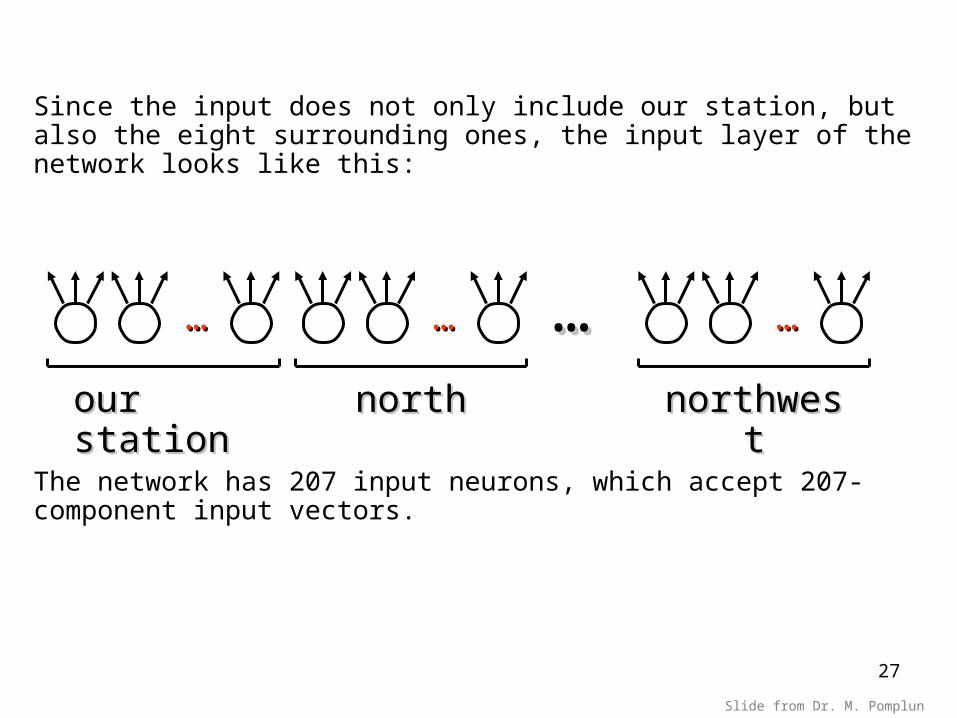
Since the input does not only include our station, but also the eight surrounding ones, the input layer of the network looks like this:

……

our stationour station

……

northnorth

…… ……

northwestnorthwest

The network has 207 input neurons, which accept 207-component input vectors.


28

What should the output patterns look like?

We want the network to produce a set of indicators that we

can interpret as a prediction of the weather in 24 hours from

now.

In analogy to the weather forecast on the evening news, we

decide to demand the following four indicators:

• a temperature prediction

• a prediction of the chance of precipitation occurring

• an indication of the expected cloud cover

• a storm indicator (extreme conditions warning)


29

Each of these four indicators can be represented by one scaled

output value:

• temperature (-10… 40 degrees Celsius)

• chance of precipitation (0%… 100%)

• cloud cover (0… 9)

• storm warning: two possibilities:

– 0: no storm warning; 1: storm warning

– probability of serious storm (0%… 100%)

Of course, the actual network outputs range from to (1 - ), and

after their computation, if necessary, they are scaled to match

the ranges specified above.


30

We decide (or experimentally determine) to use a hidden layer

with 42 sigmoidal neurons.

In summary, our network has

• 207 input neurons

• 42 hidden neurons

• 4 output neurons

Because of the small output vectors, 42 hidden units may suffice

for this application.


31

The next thing we need to do is collecting the training

exemplars.

First we have to specify what our network is supposed to do:

In production mode, the network is fed with the

current weather conditions, and its output will be

interpreted as the weather forecast for tomorrow.

Therefore, in training mode, we have to present the network with

exemplars that associate known past weather conditions at a time

t with the conditions at t – 24 hrs.

So we have to collect a set of historical exemplars with known

correct output for every input.


32

Obviously, if such data is unavailable, we have to start

collecting them.

The selection of exemplars that we need depends, among

other factors, on the amount of changes in weather at our

location.And how about the granularity of our exemplar data, i.e., the

frequency of measurement?

Using one sample per day would be a natural choice, but it

would neglect rapid changes in weather.

If we use hourly instantaneous samples, however, we

increase the likelihood of conflicts.


33

Therefore, we decide to do the following:

We will collect input data every hour, but the corresponding

output pattern will be the average of the instantaneous patterns

over a 12-hour period.

This way we reduce the possibility of errors while increasing the

amount of training data.

Now we have to train our network.

If we use samples in one-hour intervals for one year, we have

8,760 exemplars.

Our network has 20742 + 424 = 8862 weights, which means

that data from ten years, i.e., 87,600 exemplars would be

desirable (rule of thumb).


34

Since with a large number of samples the hold-one-out

training method is very time consuming, we decide to use

partial-set training instead.

The best way to do this would be to acquire a test set

(control set), that is, another set of input-output pairs

measured on random days and at random times.

After training the network with the 87,600 exemplars, we

could then use the test set to evaluate the performance of

our network.


35

Neural network troubleshooting:

Plot the global error as a function of the training epoch. The

error should decrease after every epoch. If it oscillates, do

the following tests.

• Try reducing the size of the training set. If then the network

converges, a conflict may exist in the exemplars.

• If the network still does not converge, continue pruning the

training set until it does converge. Then add exemplars back

gradually, thereby detecting the ones that cause conflicts.

• If this still does not work, look for saturated neurons (extreme weights) in the hidden layer. If you find those, add more hidden-layer neurons, possibly an extra 20%.

• If there are no saturated units and the problems still exist, try lowering the learning parameter and training longer.


36

• If the network converges but does not accurately learn the desired function, evaluate the coverage of the training set. If the coverage is adequate and the network still does not learn the function precisely, you could refine the pattern representation. For example, you could include a season indicator to the input, helping the network to discriminate between similar inputs that produce very different outputs.


1/11 طراحی و آموزش شبکه های عصبی slide from dr. m. pomplun

Documents