vtu syllabus dsp lab using compose - … · figure 3.a.1: linear convolution of two sequence . 3b:...
TRANSCRIPT
1
VTU Syllabus DSP lab using Compose
Author: Sijo George
Altair Engineering – Bangalore
(2)
2
Contents
Experiment 1: Verification of Sampling Theorem ........................................................................................ 3
Experiment 2: Impulse response of a system ............................................................................................... 5
Experiment 3: Linear Convolution of two signals ......................................................................................... 7
3a: Linear Convolution of two sequences ..................................................................................................... 7
3b: Linear Convolution using DFT/IDFT ........................................................................................................ 8
Experiment 4: Circular convolution of two given sequences ..................................................................... 10
Experiment 5: Autocorrelation of a given sequence and verification of its properties ............................. 12
Experiment 6: Solving a given difference equation. ................................................................................... 14
Software Code: ............................................................................................................................................ 14
Experiment 7: Computation of N point DFT of a given sequence and to plot magnitude and phase spectrum. .................................................................................................................................................... 16
Experiment 8: Circular convolution of two given sequences using DFT and IDFT ...................................... 18
Experiment 9: Design and implementation of IIR Butterworth filter to meet given specifications ........... 20
Table of figures
Figure 1: Verification of Sampling Theorem ................................................................................................. 4
Figure 2: Impulse Response of a system ....................................................................................................... 6
Figure 3.a.1: Linear Convolution of two sequences ...................................................................................... 8
Figure 3.b.1: Linear Convolution using DFT .................................................................................................. 9
Figure 4.1: Circular convolution of two sequence .................................................................................... 111
Figure 5.1: Auto correlation of Two Discrete Sequences ......................................................................... 133
Figure 6.1: Difference Equation .................................................................................................................. 15
Figure 7.1: Computation of N point DFT of a sequence and plotting magnitude and phase spectrum ... 177
Figure 8.1: Circular Convolution of two sequences using DFT ................................................................... 19
Figure 9.1: Frequency response of IIR butterworth digital filter ................................................................ 21
3
Experiment 1: Verification of Sampling Theorem
Description:
In this experiment the task is to understand how sampling theorem works and demonstrate the ideal sampling, under sampling as well as over sampling scenarios for a given signal
Software code:
clc;clear all;close all; T=0.04; % Time period of 50 Hz signal t=0:0.0005:0.02; f = 1/T; n1=0:40; size(n1) xa_t=sin(2*pi*2*t/T); subplot(2,2,1); plot(200*t,xa_t); title('Verification of sampling theorem'); title('Continuous signal'); xlabel('t'); ylabel('x(t)'); ts1=0.002;%>niq rate ts2=0.01;%=niq rate ts3=0.1;%<niq rate n=0:20; x_ts1=2*sin(2*pi*n*ts1/T); subplot(2,2,2); stem(n,x_ts1); title('greater than Nq'); xlabel('n'); ylabel('x(n)'); n=0:4; x_ts2=2*sin(2*pi*n*ts2/T); subplot(2,2,3); stem(n,x_ts2); title('Equal to Nq'); xlabel('n'); ylabel('x(n)'); n=0:10; x_ts3=2*sin(2*pi*n*ts3/T);
4
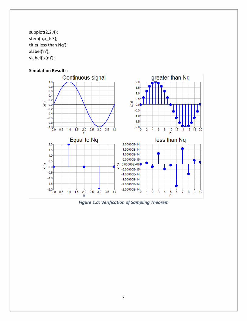
subplot(2,2,4); stem(n,x_ts3); title('less than Nq'); xlabel('n'); ylabel('x(n)'); Simulation Results:
Figure 1.a: Verification of Sampling Theorem
5
Experiment 2: Impulse response of a system
Description: Impulse response of a dynamic system is its output when presented with a brief input signal called an impulse. Since it contains all frequencies, the impulse response defines the response of a LTI system for all frequencies.
Software Code:
clc; clear all; close all;
% Difference equation of a second order system
% y(n) = x(n)+0.5x(n-1)+0.85x(n-2)+y(n-1)+y(n-2)
b=input('enter the coefficients of x(n),x(n-1)----- respectively in Matrix form');
a=input('enter the coefficients of y(n),y(n-1)---- respectively in Matrix form');
N=input('enter the number of samples of imp response ');
[h,t]=impz(b,a,N); % Function defined for finding Impulse response
stem(t,h); % Plot Impulse response
title('Impulse response of the system');
ylabel('Amplitude');
xlabel('Time index, N');
grid on;
disp(h);
%-------------Function for finding the impulse response of a system
function [h,t]=impz(b,a,N)
imp=[1 zeros(1,N-1)]; % Padding Zeros from 1 to N-1 points since impulse fn is defined only at 0.
h=filter(b,a,imp); % Finding the filter response
t=0:N-1; % Time duration for plotting purpose
end
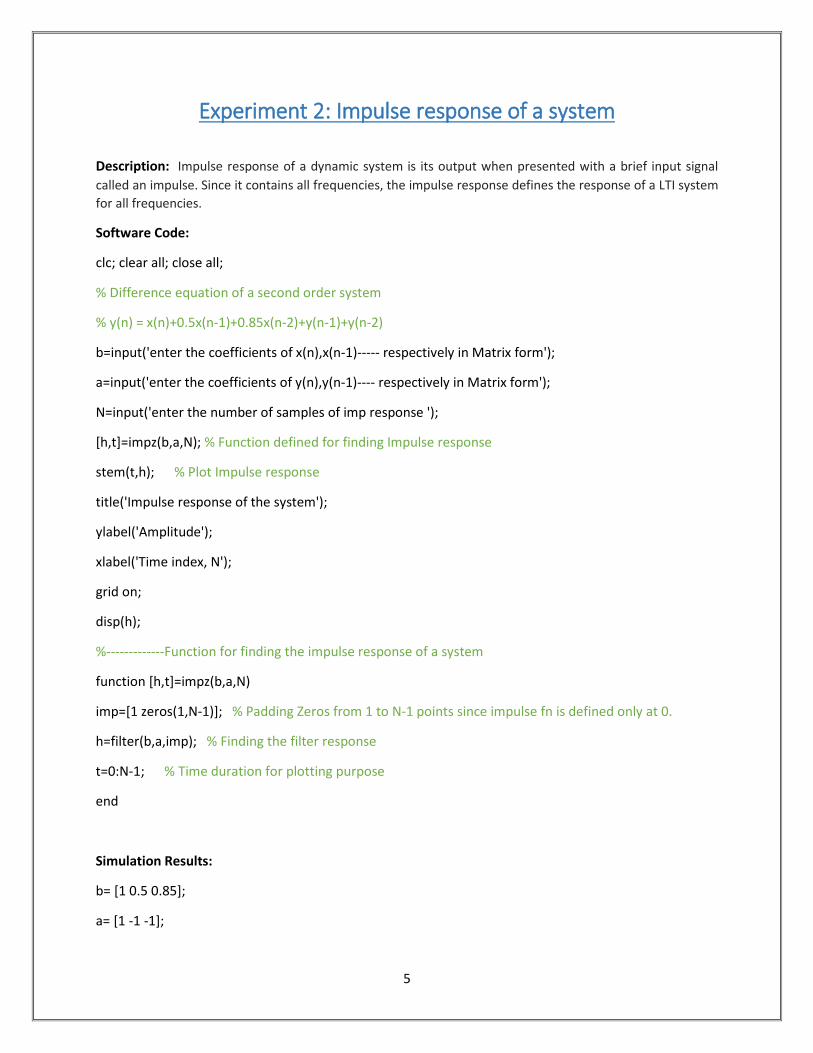
Simulation Results:
b= [1 0.5 0.85];
a= [1 -1 -1];
6
Number of samples=10;
Output sequence= [1, 1.5, 3.35, 4.85, 8.2, 13.05, 21.25, 34.3, 55.55, 89.85]
Figure 1: Impulse Response of the given system
7
Experiment 3: Linear Convolution of two signals
3a: Linear Convolution of two sequences Description: To find the convolution of two sequences using the conv function. Convolution is the mathematical operation on two functions to produce a third function which will be a modified version of one of the original function
Software Code:
clc; clear all; close all; x1=input('Enter the first sequence'); subplot(3,1,1); stem(x1); % plot for first sequence xlabel('Time index n'); ylabel('Amplitude'); title('First sequence'); grid on; x2=input('Enter 2nd sequence'); subplot(3,1,2); stem(x2); % plot for second sequence xlabel('Time index, n'); ylabel('Amplitude'); title('Second sequence'); grid on; f=conv(x1,x2); % Convolution of the two sequences disp('output of linear conv is'); disp(f); subplot(3,1,3); stem(f); % plot for convoluted sequence title('Linearly Convoluted Sequence'); xlabel('Time index, n'); ylabel('Amplitude'); grid on; Simulation Results: Sequence1: [1 2 3] Sequence2: [1 2 3 4] Out put sequence=[1, 4, 10, 16, 17, 12]

8
Figure 3.a.1: Linear Convolution of two sequence
3b: Linear Convolution using DFT/IDFT Description: To find the linear convolution of two given sequences using DFT and IDFT
Software code:
clc; close all; clear all; x1=input('Enter the first sequence:'); x2=input('Enter the second sequence:'); subplot(3,1,1); stem(x1); % Plot for first sequence title('First sequence'); xlabel('Time index, n'); ylabel('Amplitude');grid on; subplot(3,1,2); stem(x2); % Plot for second sequence title('Second sequnce'); xlabel('Time index, n'); ylabel('Amplitude');grid on; n1 = length(x1); % Length of First signal n2 = length(x2); % Length of Second signal

9
m = n1+n2-1; % Length of linear convolution x = [x1 zeros(1,n2-1)]; % Padding of zeros to make it of length m y = [x2 zeros(1,n1-1)]; x_fft = fft(x,m); % Finding dft y_fft = fft(y,m); dft_xy = x_fft.*y_fft; % Convoluted sequence in frequency domain y=ifft(dft_xy,m); % Circular convoluted sequence in discrete domain disp('The circular convolution result is ......'); disp(y); subplot(3,1,3); stem(y); % Plot for convoluted sequence title('Circularly convoluted sequence'); xlabel('Time index, n'); ylabel('Amplitude');grid on; Simulation Results:
Sequence 1:[1 2 3]
Sequence 2: [ 1 2 3 4]
Out put sequence=[1, 4, 10, 16, 17, 12]
Figure 3.b.1: Linear Convolution using DFT/IDFT
10
Experiment 4: Circular convolution of two given sequences
Description: To find the circular convolution of two given sequences. The circular convolution, also known as cyclic convolution, of two aperiodic functions occurs when one of them is convolved in the normal way with a periodic summation of the other function.
Software code:
clc; clear all; close all;
x1=input('Enter the first sequence:');
x2=input('Enter the second sequence:');
n=input('Enter the number of points:');
n1 = length(x1); % length of first signal
n2 = length(x2); % length of second signal
subplot(3,1,1);
stem(x1); % Plot for First sequence
title('First sequence');
xlabel('Time index, n');
ylabel('Amplitude');grid on;
subplot(3,1,2);
stem(x2); % Plot for Second sequence
title('Second sequence');
xlabel('Time index, n');
ylabel('Amplitude');grid on;
y1=fft(x1,n); % Finding DFT
y2=fft(x2,n);
y3=y1.*y2;
y=ifft(y3,n) %Convoluted sequence in discrete domain
disp('the circular convolution result is ......');
disp(y);
11
subplot(3,1,3);
stem(y); % Plot for convoluted sequence
title('Circular convoluted sequence');
xlabel('Time index, n');
ylabel('Amplitude');grid on;
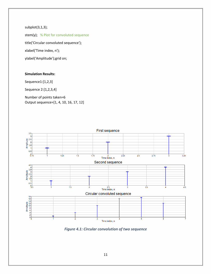
Simulation Results:
Sequence1:[1,2,3]
Sequence 2:[1,2,3,4]
Number of points taken=6 Output sequence=[1, 4, 10, 16, 17, 12]
Figure 4.1: Circular convolution of two sequence
12
Experiment 5: Autocorrelation of a given sequence and verification of its properties
Description: To find the auto correlation of two sequences. Autocorrelation, also known as serial correlation or cross-autocorrelation, is the cross-correlation of a signal with itself at different points in time (that is what the cross stands for). Informally, it is the similarity between observations as a function of the time lag between them.
Software code:
clc; close all; clf; x=[1,2,3,6,5,4]; % Input signal subplot(2,1,1) stem(x) % plot for the input sequence title('Input sequence') ylabel('Amplitude'); xlabel('Time index,n');grid on; Rxx=xcorr(x,x); % Auto correlation of the signal nRxx=-length(x)+1:length(x)-1 ; % Axis for auto correlation results subplot(2,1,2) stem(nRxx,Rxx) % plot for the auto-correlated sequence title('Auto-correlated sequence') ylabel('Amplitude'); xlabel('Time index,n');grid on; % properties :Rxx(0) gives the energy of the signal % find energy of the signal energy=sum(x.^2) centre_index=ceil(length(Rxx)/2) %set index of the center value Rxx_0=Rxx(centre_index) % Access the center value Rxx(0) % Check if the Rxx(0)=energy if Rxx_0==energy disp('Rxx(0) gives energy proved'); else disp('Rxx(0) gives energy not proved'); end Rxx_right=Rxx(centre_index:1:length(Rxx)) Rxx_left=Rxx(centre_index:-1:1) if Rxx_right==Rxx_left disp('Rxx is even'); else disp('Rxx is not even'); end
13
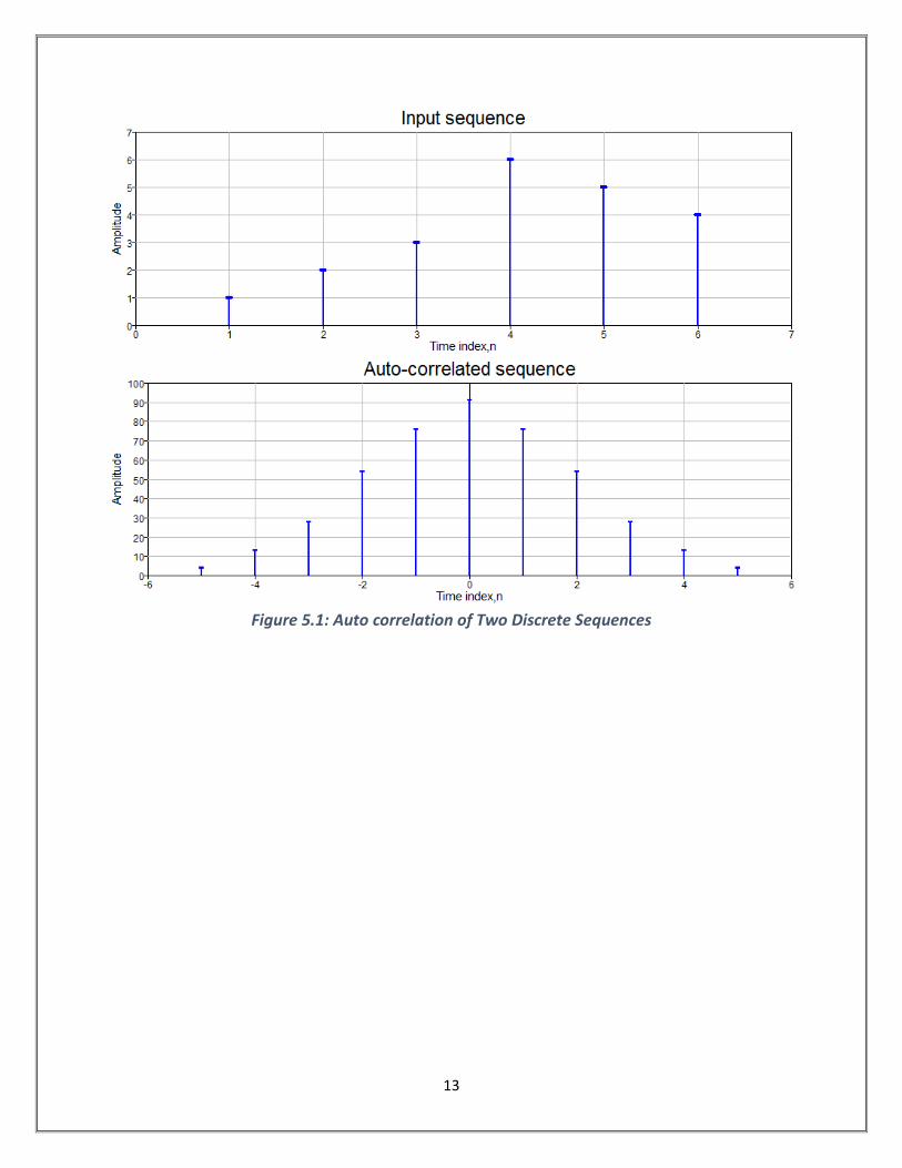
Figure 5.1: Auto correlation of Two Discrete Sequences
14
Experiment 6: Solving a given difference equation.
Description: To solve a difference equation. The difference equation is a formula for computing an output sample at time, n based on past and present input samples and past output samples in the time domain.
Software Code: clc; clear all; close all;
X = [1 2 3 4]; % input sequence
% Compute the output sequences
xcoeff = [0.5 0.27 0.77]; % x(n), x(n-1), x(n-2)… coefficients
ycoeff = [0.5 0.27 0.77];
subplot(3,1,1);
stem(X); % Plot for input sequence
xlabel('Time index,n');
ylabel('Amplitude');
title('Input sequence'); grid on;
y1 = filter(xcoeff,ycoeff,X); % Output of the filter for the given sequence
subplot(3,1,2);
stem(y1); % Plot the output sequences
xlabel('Time index,n');
ylabel('Amplitude');
title('Filtered output sequence'); grid on;
% to find out h(n) of the difference equation
% y(n)-(1/2)*y(n-1) = (1/2)*x(n)+(1/2)*x(n-1)
b=input('Enter the coefficients of x(n),x(n-1)-----');
a=input('Enter the coefficients of y(n),y(n-1)----');
N=input('Enter the number of samples of imp response');
[h,t]=impz(b,a,N); % Function defined for finding Impulse response (Details in Exp.2)
subplot(3,1,3)
stem(t,h);
15
title('plot of impulse response');
ylabel('amplitude');
xlabel('time index----->N');
disp(h); grid on;
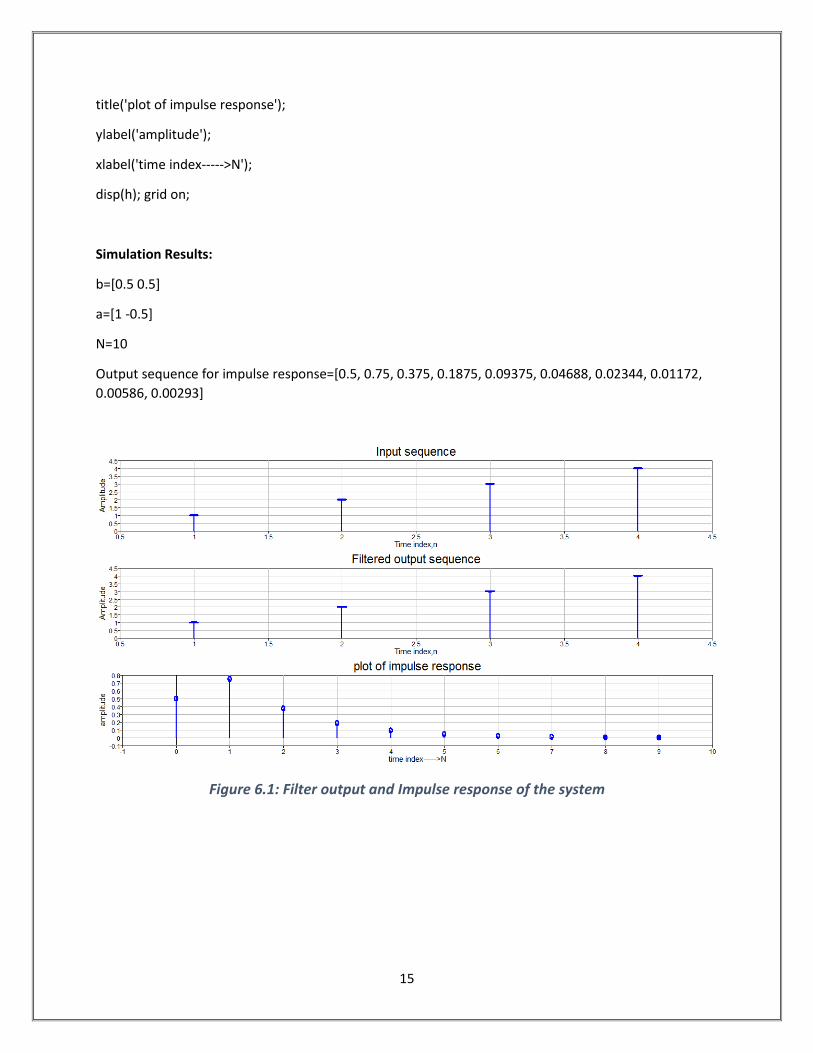
Simulation Results:
b=[0.5 0.5]
a=[1 -0.5]
N=10
Output sequence for impulse response=[0.5, 0.75, 0.375, 0.1875, 0.09375, 0.04688, 0.02344, 0.01172, 0.00586, 0.00293]
Figure 6.1: Filter output and Impulse response of the system
16
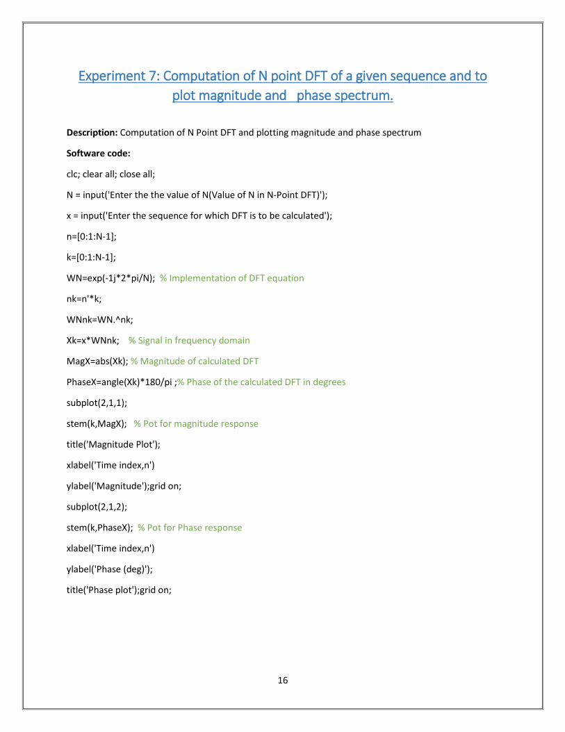
Experiment 7: Computation of N point DFT of a given sequence and to plot magnitude and phase spectrum.
Description: Computation of N Point DFT and plotting magnitude and phase spectrum
Software code:
clc; clear all; close all;
N = input('Enter the the value of N(Value of N in N-Point DFT)');
x = input('Enter the sequence for which DFT is to be calculated');
n=[0:1:N-1];
k=[0:1:N-1];
WN=exp(-1j*2*pi/N); % Implementation of DFT equation
nk=n'*k;
WNnk=WN.^nk;
Xk=x*WNnk; % Signal in frequency domain
MagX=abs(Xk); % Magnitude of calculated DFT
PhaseX=angle(Xk)*180/pi ;% Phase of the calculated DFT in degrees
subplot(2,1,1);
stem(k,MagX); % Pot for magnitude response
title('Magnitude Plot');
xlabel('Time index,n')
ylabel('Magnitude');grid on;
subplot(2,1,2);
stem(k,PhaseX); % Pot for Phase response
xlabel('Time index,n')
ylabel('Phase (deg)');
title('Phase plot');grid on;
17
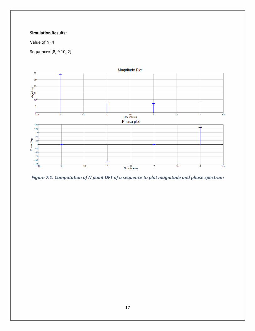
Simulation Results:
Value of N=4
Sequence= [8, 9 10, 2]
Figure 7.1: Computation of N point DFT of a sequence to plot magnitude and phase spectrum

18
Experiment 8: Circular convolution of two given sequences using DFT and IDFT
Description: To find the circular convolution of two given sequences using DFT and IDFT
Software Code:
clc; close all; clear all;
x1=input('Enter the first sequence:');
x2=input('Enter the second sequence:');
n=input('Enter the no of points of the DFT:');
subplot(3,1,1);
stem(x1); % First sequence plot
title('First sequence');
xlabel('Time index,n')
ylabel('Amplitude');grid on;
subplot(3,1,2);
stem(x2); % Second sequence plot
title('Second sequence');
xlabel('Time index,n')
ylabel('Amplitude');grid on;
y1=fft(x1,n); %Finding DFT
y2=fft(x2,n);
y3=y1.*y2;
y=ifft(y3,n); % Convoluted sequence in discrete time domain
disp('The circular convolution result is: ');
disp(y);
subplot(3,1,3);
stem(y); % Convoluted sequence plot
title('Circularly convoluted sequence');
xlabel('Time index,n');
19
ylabel('Amplitude');grid on;
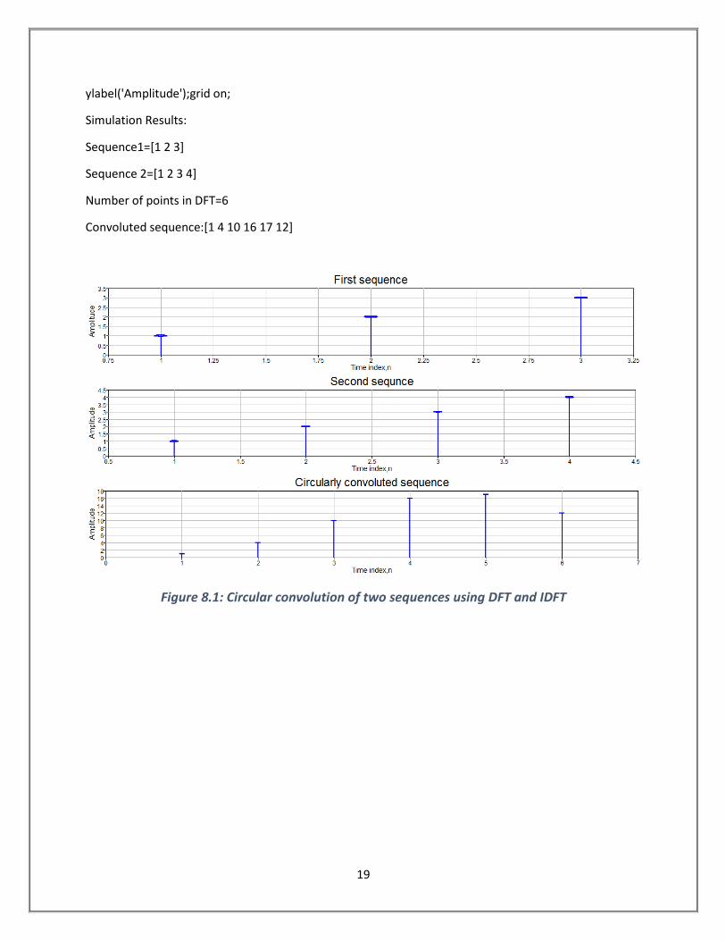
Simulation Results:
Sequence1=[1 2 3]
Sequence 2=[1 2 3 4]
Number of points in DFT=6
Convoluted sequence:[1 4 10 16 17 12]
Figure 8.1: Circular convolution of two sequences using DFT and IDFT
20
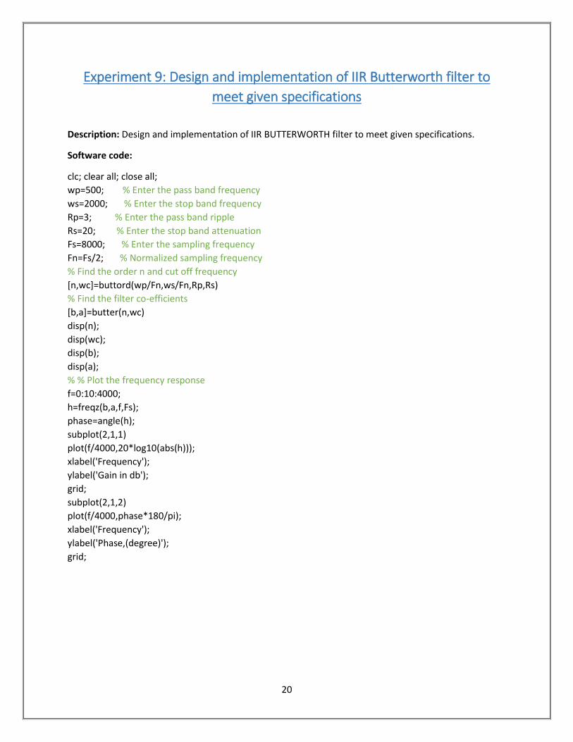
Experiment 9: Design and implementation of IIR Butterworth filter to meet given specifications
Description: Design and implementation of IIR BUTTERWORTH filter to meet given specifications.
Software code:
clc; clear all; close all; wp=500; % Enter the pass band frequency ws=2000; % Enter the stop band frequency Rp=3; % Enter the pass band ripple Rs=20; % Enter the stop band attenuation Fs=8000; % Enter the sampling frequency Fn=Fs/2; % Normalized sampling frequency % Find the order n and cut off frequency [n,wc]=buttord(wp/Fn,ws/Fn,Rp,Rs) % Find the filter co-efficients [b,a]=butter(n,wc) disp(n); disp(wc); disp(b); disp(a); % % Plot the frequency response f=0:10:4000; h=freqz(b,a,f,Fs); phase=angle(h); subplot(2,1,1) plot(f/4000,20*log10(abs(h))); xlabel('Frequency'); ylabel('Gain in db'); grid; subplot(2,1,2) plot(f/4000,phase*180/pi); xlabel('Frequency'); ylabel('Phase,(degree)'); grid;

21
Simulation results
Figure 9.1: Frequency Response of Butterworth IIR digital filter