basic filters (7) - swarthmore · pdf filebasic filters (7) –...
TRANSCRIPT

Basic Filters (7) – Convolution/correlation/Linear filtering – Gaussian filters – Smoothing and noise reduction – First derivatives of Gaussian – Second derivative of Gaussian: Laplacian – Oriented Gaussian filters – Steerability

Convolution • 1D Formula:
• 2D Formula:
• Example on the web: – http://www.jhu.edu/~signals/convolve/


1/9 1/9 1/9
1/9 1/9 1/9
1/9 1/9 1/9
Kernel:

0.04
0.04
0.04
0.04
0.04
0.04
0.04
0.04
0.04
0.04
0.04
0.04
0.04
0.04
0.04
0.04
0.04
0.04
0.04
0.04
0.04
0.04
0.04
0.04
0.04
Kernel:

Kernel: 15 x 15
matrix of value 1/225

Basic Properties
• Commutes: f * g = g * f • Associative: (f * g) * h = f * (g * h) • Linear: (af + bg) * h = a f * h + b g * h • Shift invariant: ft * h = (f * h)t
• Only operator both linear and shift invariant • Differentiation:

Practicalities (discrete convolution/correlation) • MATLAB: conv (1D) or conv2
(2D), corr • Border issues:
– When applying convolution with a KxK kernel, the result is undefined for pixels closer than K pixels from the border of the image
• Options:
K
Warp around Expand/Pad
Crop

1-D:
2-D:
Slight abuse of notations: We ignore the normalization constant such that

, ! = 5
Kernel:

Simple Averaging
Gaussian Smoothing

Image Noise

Gaussian Smoothing to Remove Noise
! = 2 ! = 4 No smoothing

! = 1
! = 3
! = 5
Shape of Gaussian filter as function of !"

• Gaussian function has infinite support
• In discrete filtering, we have finite kernel size
Note about Finite Kernel Support

Increasing !"
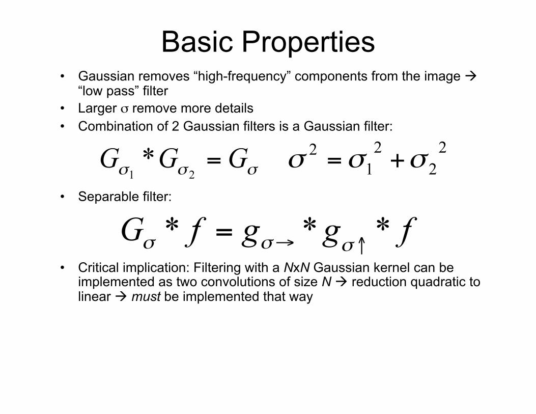
Basic Properties • Gaussian removes “high-frequency” components from the image !
“low pass” filter • Larger ! remove more details • Combination of 2 Gaussian filters is a Gaussian filter:
• Separable filter:
• Critical implication: Filtering with a NxN Gaussian kernel can be implemented as two convolutions of size N ! reduction quadratic to linear ! must be implemented that way
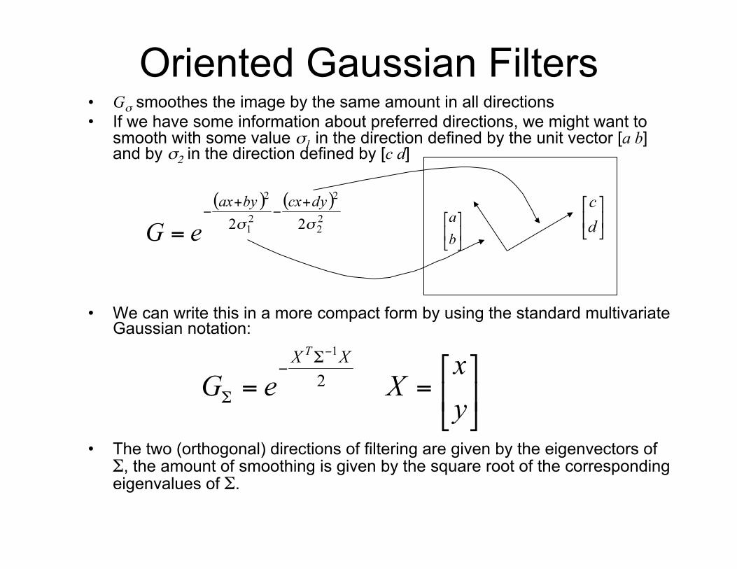
Oriented Gaussian Filters • G! smoothes the image by the same amount in all directions • If we have some information about preferred directions, we might want to
smooth with some value !1 in the direction defined by the unit vector [a b] and by !2 in the direction defined by [c d]
• We can write this in a more compact form by using the standard multivariate Gaussian notation:
• The two (orthogonal) directions of filtering are given by the eigenvectors of #, the amount of smoothing is given by the square root of the corresponding eigenvalues of #.


Image Derivatives
• Image Derivatives • Derivatives increase noise • Derivative of Gaussian • Laplacian of Gaussian (LOG)

Image Derivatives
Difference between Actual image values
True difference (derivative)
Twice the amount of noise as in the original image
• We want to compute, at each pixel (x,y) the derivatives: • In the discrete case we could take the difference
between the left and right pixels:
• Convolution of the image by
• Problem: Increases noise
-1 0 1

Orig
inal
Imag
e Noise A
dded
Derivative in the horizontal direction

Smooth Derivatives • Solution: First smooth the image by a Gaussian G! and then take
derivatives:
• Applying the differentiation property of the convolution:
• Therefore, taking the derivative in x of the image can be done by convolution with the derivative of a Gaussian:
• Crucial property: The Gaussian derivative is also separable:

G
Gx

Derivative + Smoothing
Better but still blurs away edge information
Without smoothing With smoothing

Applying the first derivative of Gaussian
I

Input
Difference operator
Derivative from difference operator
Gaussian derivative operator
Derivative from Gaussian derivative

There is ALWAYS a tradeoff between smoothing and good edge localization!
Image with Edge Edge Location
Image + Noise Derivatives detect edge and noise
Smoothed derivative removes noise, but blurs edge

g
gxx
Second derivatives: Laplacian

DOG Approximation to LOG

Separable, low-pass filter
Not-separable, approximated by A difference of Gaussians. Output of convolution is Laplacian of image: Zero-crossings correspond to edges
Separable, output of convolution is gradient at scale !:
Gaussian
Derivatives of Gaussian
Directional Derivatives
Laplacian
Output of convolution is magnitude of derivative in direction $. Filter is linear combination of derivatives in x and y
Oriented Gaussian
Smooth with different scales in orthogonal directions

Edge Detection • Edge Detection
– Gradient operators – Canny edge detectors – Laplacian detectors

What is an edge?
Edge = discontinuity of intensity in some direction. Could be detected by looking for places where the derivatives of the image have large values.

$
Edge pixels are at local maxima of gradient magnitude Gradient computed by convolution with Gaussian derivatives Gradient direction is always perpendicular to edge direction

Small sigma Large sigma

!= 10 != 1
Large ! ! Good detection (high SNR) Poor localization
Small ! ! Poor detection (low SNR) Good localization

Canny’s Result • Given a filter f, define the two objective functions:
%(f) large if f produces good localization #(f) large if f produces good detection (high SNR)
• Problem: Find a family of filters f that maximizes the compromise criterion %(f)#(f) under the constraint that a single peak is generated by a step edge • Solution: Unique solution, a close approximation is the Gaussian derivative
filter!
Canny Derivative of Gaussian

Next Steps • The gradient magnitude enhances the edges but 2
problems remain: – What threshold should we use to retain only the “real” edges? – Even if we had a perfect threshold, we would still have poorly
localized edges. How to extract optimally localize contours? • Solution: Two standard tools:
– Non-local maxima suppression – Hysteresis thresholding
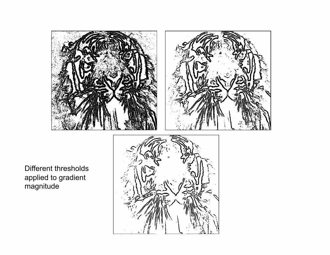
Different thresholds applied to gradient magnitude

Input image

Different thresholds applied to gradient magnitude

Non-Local Maxima Suppression
1.5
2
2
4.1
Gradient magnitude at center pixel is lower than the gradient magnitude of a neighbor in the direction of the gradient ! Discard center pixel (set magnitude to 0)
Gradient magnitude at center pixel is greater than gradient magnitude of all the neighbors in the direction of the gradient ! Keep center pixel unchanged
2.5
1.0

T = 15 T = 5
Two thresholds applied to gradient magnitude

Weak pixels but connected
Very strong edge response. Let’s start here
Weaker response but it is connected to a confirmed edge point. Let’s keep it.
Continue….
Note: Darker squares illustrate stronger edge response (larger M)
Weak pixels but isolated
Hysteresis Thresholding

T=15 T=5
Hysteresis Th=15 Tl = 5
Hysteresis thresholding


Summary • Edges are discontinuities of intensity in images • Correspond to local maxima of image gradient • Gradient computed by convolution with derivatives of
Gaussian • General principle applies:
– Large !: Poor localization, good detection – Small !: Good localization, poor detection
• Canny showed that Gaussian derivatives yield good compromise between localization and detection
• Edges correspond to zero-crossings of the second derivative (Laplacian in 2-D)