Data smoothing

Raymond Cuijpers

Index

• The moving average

• Convolution

• The difference operator

• Fourier transforms

• Gaussian smoothing

• Butterworth filters

0

1/3

i i+1i-1

Si

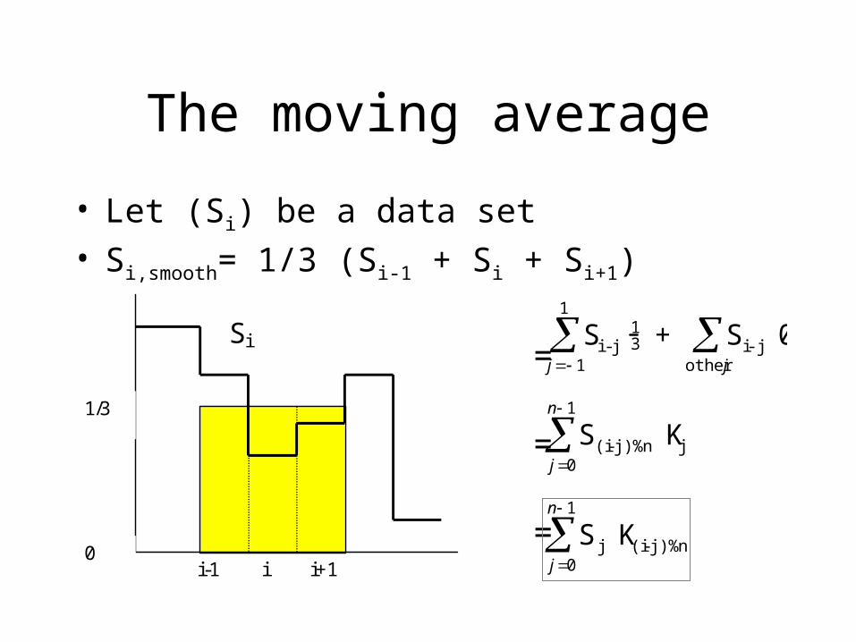
The moving average

• Let (Si) be a data set• Si,smooth= 1/3 (Si-1 + Si + Si+1)

=

=

=

Si - j 13

j 1

1

+ Si- j 0other j

S(i - j)%n Kjj 0

n 1

S j K(i - j)%nj 0

n 1

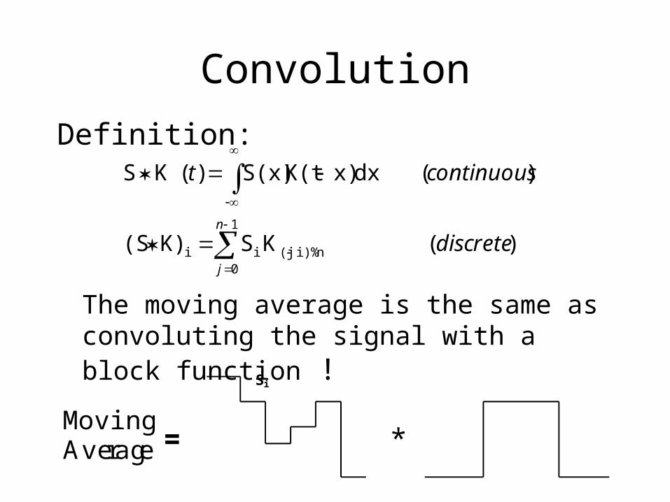
Convolution

Definition:

The moving average is the same as convoluting the signal with a block function !

S K (t) S(x)

K(t x)dx (continuous )

(S K)i Si K(j i)% nj0

n 1

(discrete )

Si

*MovingAverage =

Convolution

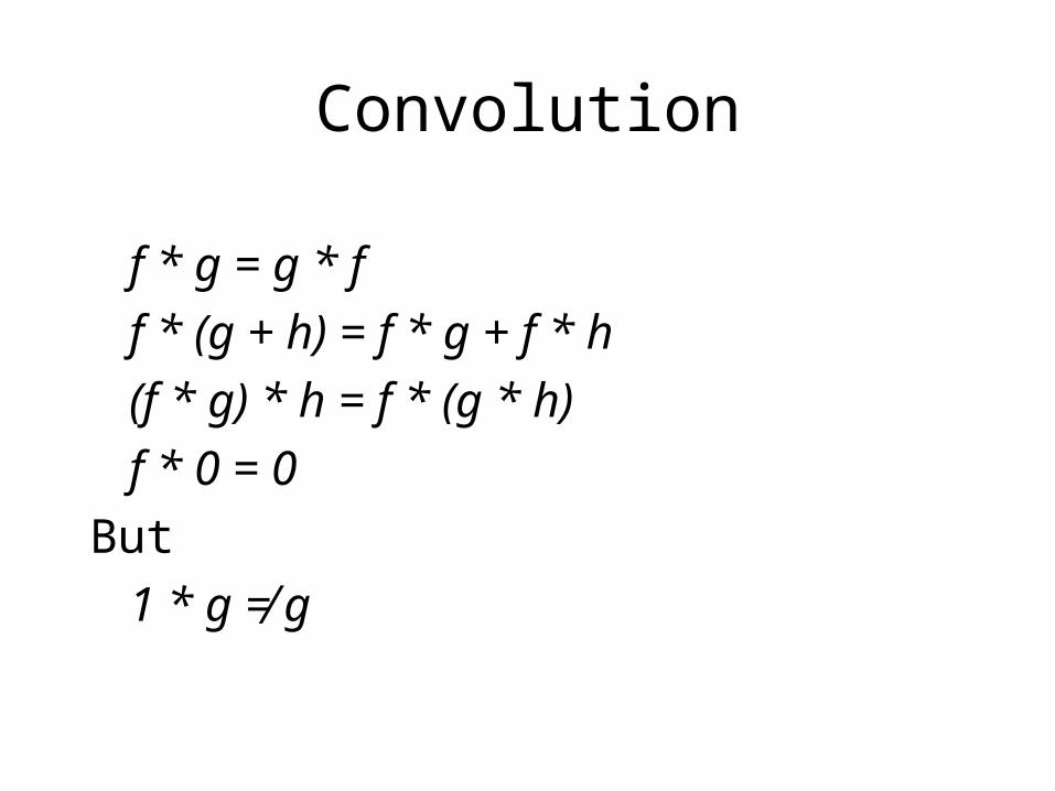
f * g = g * f

f * (g + h) = f * g + f * h

(f * g) * h = f * (g * h)

f * 0 = 0

But

1 * g ≠ g

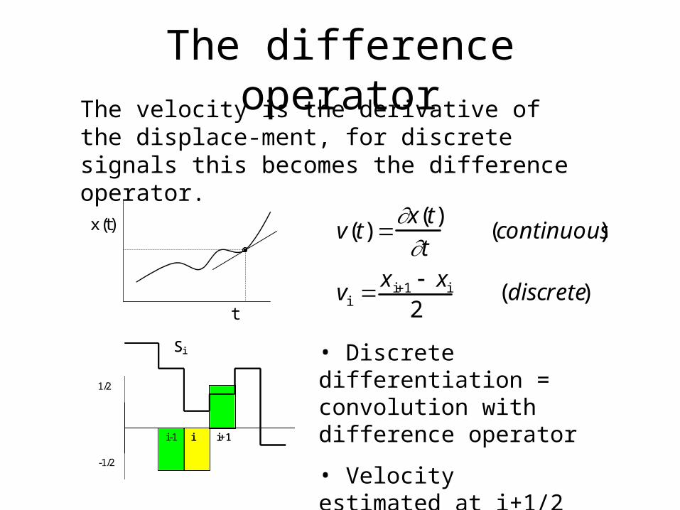
The difference operatorThe velocity is the derivative of the displace-ment, for discrete signals this becomes the difference operator.

x(t)

t

v(t) x(t)

t(continuous )

vi x i1 xi

2(discrete )

-1/2

1/2

i i+1

Si • Discrete differentiation = convolution with difference operator

• Velocity estimated at i+1/2i

-1/2

1/2

i+1

Si

i-1

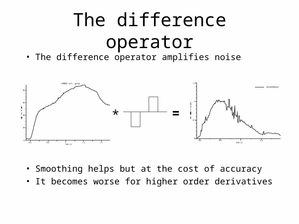
The difference operator• The difference operator amplifies noise

• Smoothing helps but at the cost of accuracy

• It becomes worse for higher order derivatives

0.6 0.8 1 1.2 1.4time (s)

0

20

40

60

80

c#002.rc1, grip

* =

0.6 0.8 1 1.2time (s)

0

0.5

1

1.5

massamiddelpunt

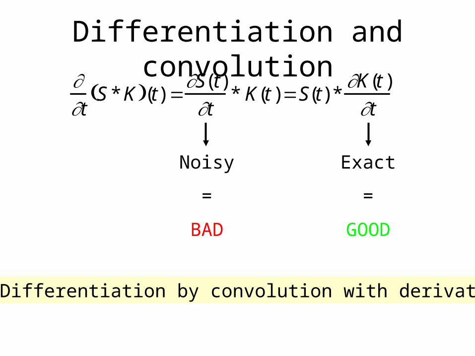
Differentiation and convolutiont

S * K (t) S( t)

t* K(t ) S(t) *

K(t )

t

Noisy

=

BAD

Exact

=

GOOD

• Differentiation by convolution with derivative

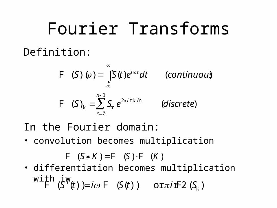
Fourier TransformsDefinition:

In the Fourier domain:• convolution becomes multiplication

• differentiation becomes multiplication with iw

F (S)() S(t)e i tdt

(continuous )

F (S)k Sr e2 i r k / n

r0

n 1

(discrete )

F (S K) F (S)F (K)

F (S' (t)) i F (S(t)) or 2 irF (Sk )

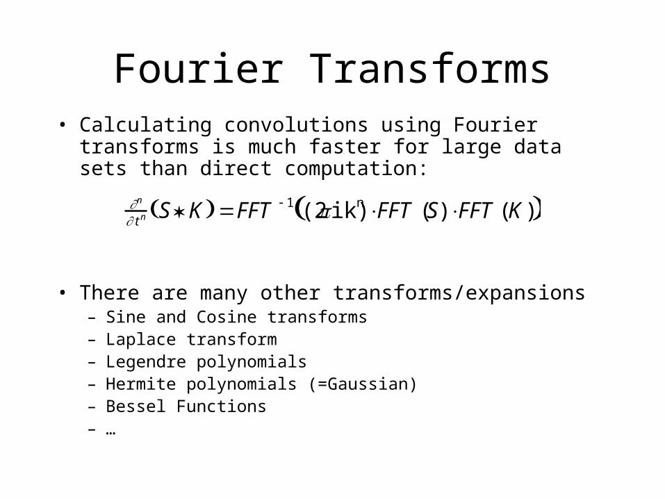
Fourier Transforms• Calculating convolutions using Fourier transforms is much

faster for large data sets than direct computation:

• There are many other transforms/expansions– Sine and Cosine transforms– Laplace transform– Legendre polynomials – Hermite polynomials (=Gaussian)– Bessel Functions– …

n

t n S K FFT 1 (2ik)n FFT (S) FFT (K)

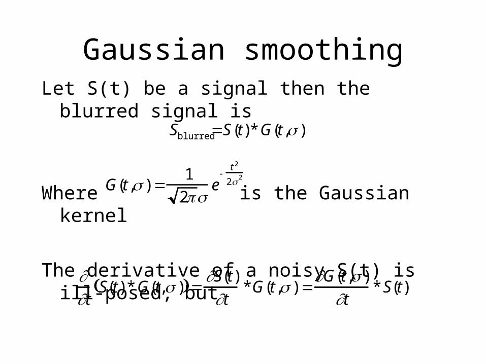
Gaussian smoothingLet S(t) be a signal then the blurred signal is

Where is the Gaussian kernel

The derivative of a noisy S(t) is ill-posed, but

G(t, ) 1

2e

t 2

2 2

t

S(t) * G(t, ) S(t)

t*G(t, )

G(t, )

t* S(t)

Sblurred S(t)* G(t, )

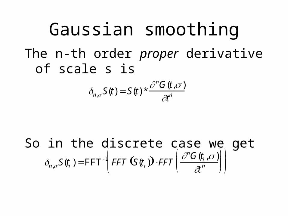
Gaussian smoothingThe n-th order proper derivative of scale s is

So in the discrete case we get

n, S(t) S(t) * nG(t, )

tn

n , S(ti ) FFT -1 FFT S(t i) FFTnG(ti , )

t n

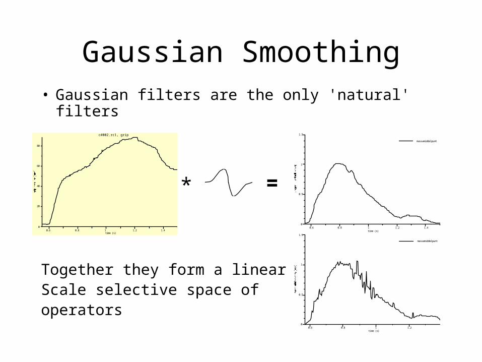
Gaussian Smoothing• Gaussian filters are the only 'natural' filters

Together they form a linearScale selective space of operators

0.6 0.8 1 1.2 1.4time (s)

0

20

40

60

80

c#002.rc1, grip

* =

0.6 0.8 1 1.2time (s)

0

0.5

1

1.5

massamiddelpunt

0.6 0.8 1 1.2 1.4time (s)

0

0.5

1

1.5

massamiddelpunt

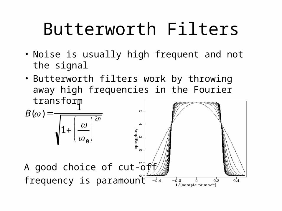
Butterworth Filters• Noise is usually high frequent and not the signal• Butterworth filters work by throwing away high

frequencies in the Fourier transform

A good choice of cut-off

frequency is paramount

B() 1

1 0

2n

Butterworth filtersAdvantage:• Easy to implement in electronic circuit

Disadvantage:• Introduces a phase shift. Solution is to apply it

twice in opposite directions• 'Ringing': jumps in the signal produces oscillations• Depends strongly on the nature of the noise and

the choice of cut-off frequency