design of fir filters - information engineering … convolution using circular convolution 14 proof...
TRANSCRIPT

1
Design of FIR Filters
Elena Punskayawww-sigproc.eng.cam.ac.uk/~op205
Some material adapted from courses by Prof. Simon Godsill, Dr. Arnaud Doucet,
Dr. Malcolm Macleod and Prof. Peter Rayner
2
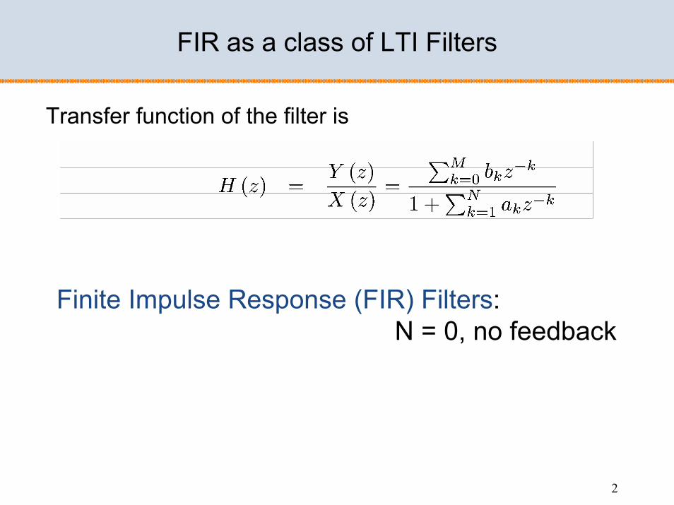
FIR as a class of LTI Filters
Transfer function of the filter is
Finite Impulse Response (FIR) Filters: N = 0, no feedback

3
FIR Filters
Let us consider an FIR filter of length M (order N=M-1, watch out! order – number of delays)
xn
yn
b0 bM
= unit delay

4
Can immediately obtain the impulse response, with x(n)= δ(n)
The impulse response is of finite length M, as required
Note that FIR filters have only zeros (no poles). Hence known also as all-zero filters
FIR filters also known as feedforward or non-recursive, or transversal
FIR filters
δ

5
FIR Filters
Digital FIR filters cannot be derived from analog filters –rational analog filters cannot have a finite impulse response.
Why bother?
1. They are inherently stable2. They can be designed to have a linear phase3. There is a great flexibility in shaping their magnitude
response4. They are easy and convenient to implement
Remember very fast implementation using FFT?

6
FIR Filter using the DFT
FIR filter:
Can we use DFT and then IDFT to compute standard convolution product and thus to perform linear filtering (given how efficient FFT is)?

7
Circular Convolution
circular convolution

8
Example of Circular Convolution
1
20
3
5 4
Circular convolution of x1={1,2,0} and x2={3,5,4}clock-wise anticlock-wise
1
20
3
5 4
1
20
5
4 3
1
20
4
3 50 spins 1 spin 2 spins
x1(n)x2(2-n)|mod3
y(0)=1×3+2×4+0×5 y(1)=1×5+2×3+0×4 y(2)=1×4+2×5+0×3
folded sequence
x1(n)x2(0-n)|mod3 x1(n)x2(1-n)|mod3
…

9
Example of Circular Convolution
clock-wise anticlock-wise
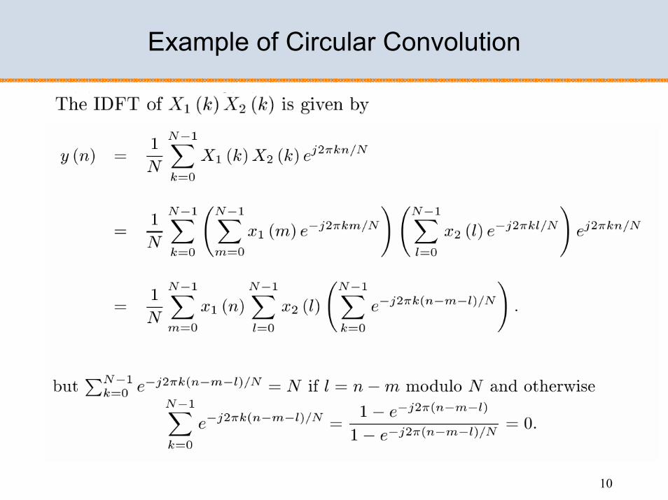
10
Example of Circular Convolution

11
Standard Convolution using Circular Convolution
12
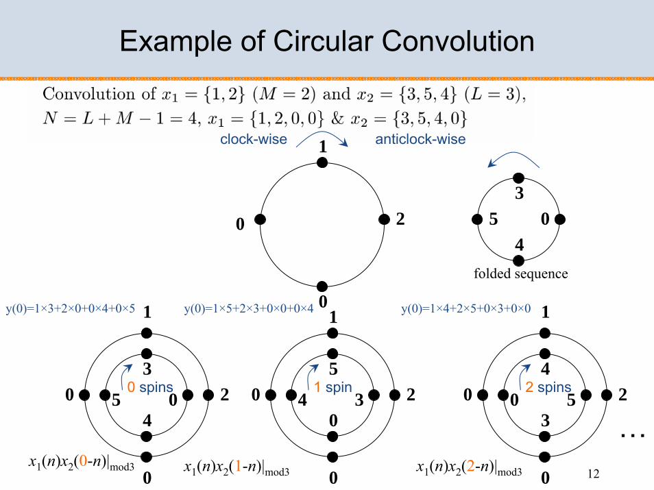
Example of Circular Convolution
1
203
5 0
clock-wise anticlock-wise1
23
5 0
0 spins
y(0)=1×3+2×0+0×4+0×5
folded sequence
x1(n)x2(0-n)|mod3 x1(n)x2(1-n)|mod3 x1(n)x2(2-n)|mod3
…
04
4
0
1
205
4 31 spin
0
0
1
204
0 52 spins
3
0
0y(0)=1×5+2×3+0×0+0×4 y(0)=1×4+2×5+0×3+0×0

13
Standard Convolution using Circular Convolution

14
Proof of Validity
Circular convolution of the padded sequence corresponds to the standard convolution

15
Linear Filtering using the DFT
FIR filter:
DFT and then IDFT can be used to compute standard convolution product and thus to perform linear filtering (given how efficient FFT is)!
Frequency domain equivalent:
16
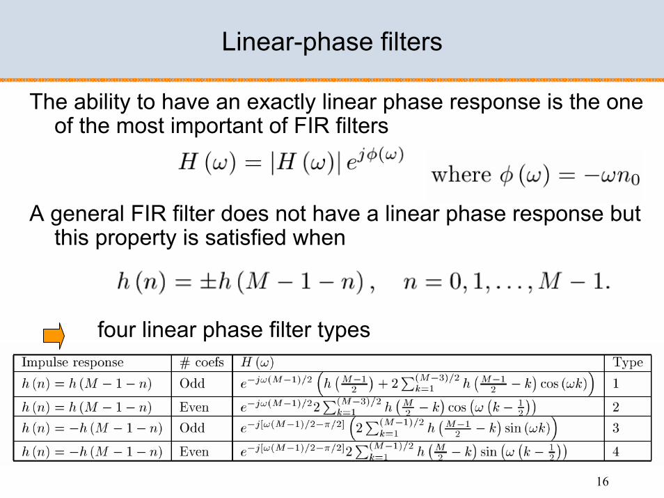
Linear-phase filters
The ability to have an exactly linear phase response is the one of the most important of FIR filters
A general FIR filter does not have a linear phase response but this property is satisfied when
four linear phase filter types

17
Linear-phase filters – Filter types
Some observations:
• Type 1 – most versatile
• Type 2 – frequency response is always 0 at ω=π – not suitable as a high-pass
• Type 3 and 4 – introduce a π/2 phase shift, frequency response is always 0 at ω=0 - – not suitable as a high-pass
18
FIR Design Methods
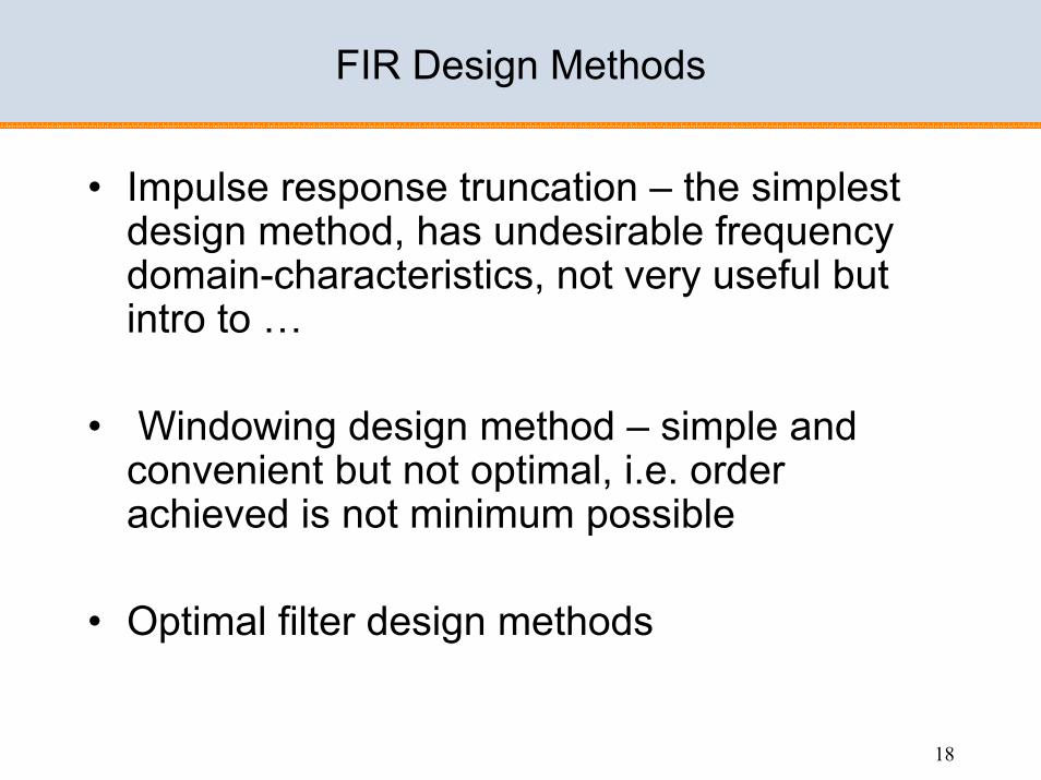
• Impulse response truncation – the simplest design method, has undesirable frequency domain-characteristics, not very useful but intro to …
• Windowing design method – simple and convenient but not optimal, i.e. order achieved is not minimum possible
• Optimal filter design methods

19
Back to Our Ideal Low- pass Filter Example

20
Approximation via truncation
M
M

21
Approximated filters obtained by truncation
transition band
M
M
M M
M
22
Window Design Method
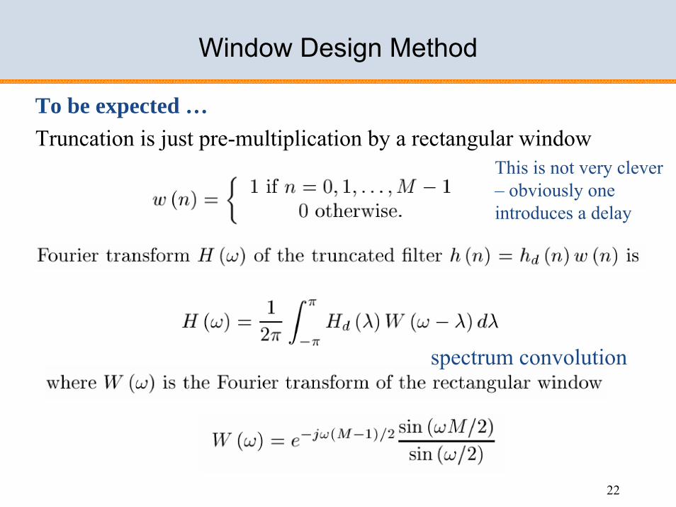
To be expected …Truncation is just pre-multiplication by a rectangular window
spectrum convolution
This is not very clever – obviously one introduces a delay

23
Rectangular Window Frequency Response
24
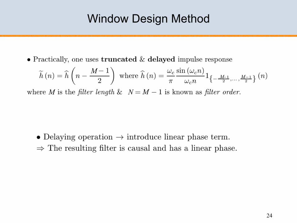
Window Design Method
M
M MN
M M

25
Magnitude of Rectangular Window Frequency Response

26
Truncated Filter

27
Truncated Filter

28
Ideal Requirements
Ideally we would like to have • small – few computations• close to a delta Dirac mass for
to be close to
These two requirements are conflicting!
our ideal low-pass filter

29
Increasing the dimension of the window
• The width of the main lobe decreases as M increases
M M
M M
M

30
Conflicting Ideal Requirements

31
Approximated filters obtained by truncation
transition bandtransition band
M
M
M M
M

32
Solution to Sharp Discontinuity of Rectangular Window
Use windows with no abrupt discontinuity in their time-domain response and consequently low side-lobes in their frequency response.
In this case, the reduced ripple comes at the expense of a wider transition region but this
However, this can be compensated for by increasing the length of the filter.

33
Alternative Windows –Time Domain
• Hanning• Hamming• Blackman
Many alternatives have been proposed, e.g.

34
Windows –Magnitude of Frequency Response

35
Summary of Windows Characteristics
We see clearly that a wider transition region (wider main-lobe) is compensated by much lower side-lobes and thus less ripples.
36
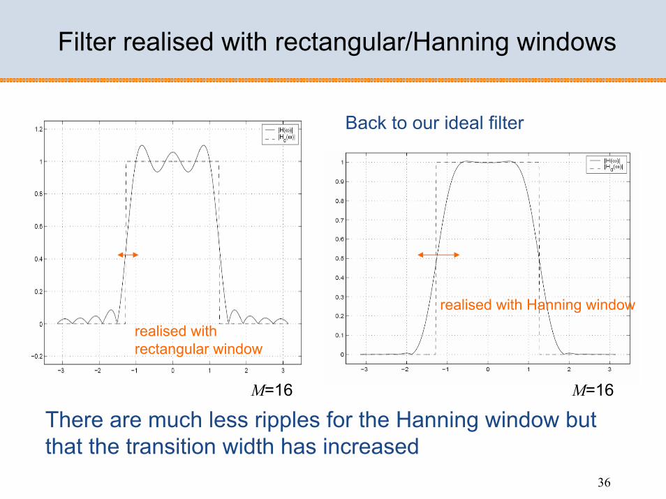
Filter realised with rectangular/Hanning windows
Back to our ideal filter
realised with rectangular window
realised with Hanning window
There are much less ripples for the Hanning window but that the transition width has increased
M=16M=16

37
Transition width can be improved by increasing the size of the Hanning window to M = 40
realised with Hanning windowM=40
realised with Hanning windowM=16
Filter realised with Hanning windows
38
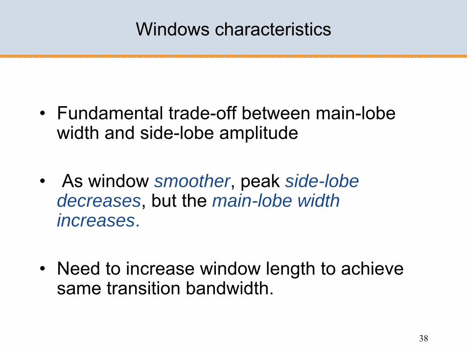
Windows characteristics
• Fundamental trade-off between main-lobe width and side-lobe amplitude
• As window smoother, peak side-lobe decreases, but the main-lobe width increases.
• Need to increase window length to achieve same transition bandwidth.

39
Specification necessary for Window Design Method
Response must not enter shaded regions
ωc - cutoff frequency
δ - maximum passbandripple
Δω – transition bandwidth
Δωm – width of the window mainlobe

40
Key Property 1 of the Window Design Method

41
Key Property 2 of the Window Design Method

42
Key Property 3 of the Window Design Method

43
Key Property 4 of the Window Design Method
44
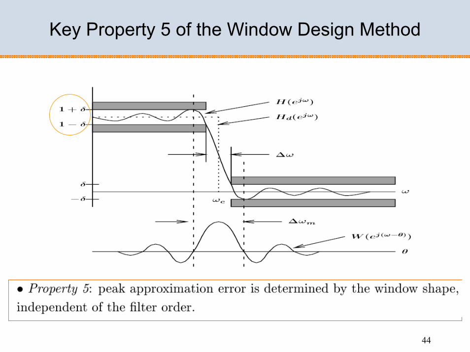
Key Property 5 of the Window Design Method

45
Passband / stopband ripples
Passband / stopband ripples are often expressed in dB:
passband ripple = 20 log10 (1+δp ) dB, or peak-to-peak passband ripple ≅ 20 log10 (1+2δp) dB;minimum stopband attenuation = -20 log10 (δs ) dB.
Example: δp= 6% peak-to-peak passband ripple ≅ 20 log10 (1+2δp) = 1dB;
δs = 0.01 minimum stopband attenuation = -20 log10 (δs) = 40dB.
The band-edge frequencies ωs and ωp are often called corner frequencies, particularly when associated with specified gain or attenuation (e.g. gain = -3dB).

46
Summary of Window Design Procedure
• Ideal frequency response has infinite impulse response
• To be implemented in practice it has to be – truncated– shifted to the right (to make is causal)
• Truncation is just pre-multiplication by a rectangular window– the filter of a large order has a narrow transition band– however, sharp discontinuity results in side-lobe
interference independent of the filter’s order and shape Gibbs phenomenon
• Windows with no abrupt discontinuity can be used to reduce Gibbs oscillations (e.g. Hanning, Hamming, Blackman)

47
1. Equal transition bandwidth on both sides of the ideal cutoff frequency.
2. Equal peak approximation error in the pass-band and stop-band.
3. Distance between approximation error peaks is approximately equal to the width of the window main-lobe.
4. The width of the main-lobe is wider than the transition band.
Summary of the Key Properties of the Window Design Method
5. Peak approximation error is determined by the window shape, independent of the filter order.
transition bandwidth
approximation error peaks
mainlobewidth

48
Summary of the windowed FIR filter design procedure
1. Select a suitable window function
2. Specify an ideal response Hd(ω)
3. Compute the coefficients of the ideal filter hd(n)
4. Multiply the ideal coefficients by the window function to give the filter coefficients
5. Evaluate the frequency response of the resulting filter and iterate if necessary (typically, it means increase M if the constraints you have been given have not been satisfied)

49
Step by Step Windowed Filter Design Example
ωp =0.2πωs =0.3πδ1 =0.01 δ2 =0.01
Design a type I low-pass filter according to the specification
passband frequency
stopband frequency

50
Step 1. Select a suitable window function
Choosing a suitable window function can be done with the aid of published data such as
The required peak error spec δ2 = 0.01, i.e. -20log10 (δs ) = - 40 dBHanning window
Main-lobe width ωs- ωp = 0.3π−0.2π = 0.1π, i.e. 0.1π = 8π / M filter length M ≥ 80, filter order N ≥ 79
Type-I filter have even order N = 80although for Hanning window first and last ones are 0 so only 78 in reality

51
Step 2 Specify the Ideal Response
Property 1: The band-edge frequency of the ideal response if the midpoint between ωs and ωp
ωc = (ωs + ωp)/2 = (0.2π+0.3π)/2 = 0.25π
our ideal low-pass filter frequency response
1 if |ω| ≤ 0.25π0 if 0.25π < |ω|< π

52
Step 3 Compute the coefficients of the ideal filter
• The ideal filter coefficients hd are given by the Inverse Discrete time Fourier transform of Hd(ω)
• Delayed impulse response (to make it causal)N
• Coefficients of the ideal filter
4040

53
Step 3 Compute the coefficients of the ideal filter
• For our example this can be done analytically, but in general (for more complex Hd (ω) functions) it will be computed approximately using an N-point InverseFast Fourier Transform (IFFT).
• Given a value of N (choice discussed later), create a sampled version of Hd (ω):
Hd(p) = Hd(2πp/N), p=0,1,...N-1.
[ Note frequency spacing 2π/N rad/sample ]

54
If the Inverse FFT, and hence the filter coefficients, are to be purely real-valued, the frequency response must be conjugate symmetric:
Hd(-2πp/N) = Hd* (2πp/N) (1)
Since the Discrete Fourier Spectrum is also periodic, we see that
Hd(-2πp/N) = Hd(2π - 2πp/N) = Hd(2π(N-p)/N) (2)
Equating (1) & (2) we must set Hd(N-p) = Hd* (p) for p = 1, ..., (N/2-1).
The Inverse FFT of Hd*(p) is an N-sample time domain function h´(n).
For h´(n) to be an accurate approximation of h(n), N must be made large enough to avoid time-domain aliasing of h(n), as illustrated below.
Step 3 Compute the coefficients of the ideal filter
55
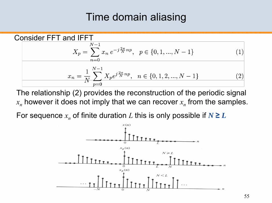
Time domain aliasing
Consider FFT and IFFT
The relationship (2) provides the reconstruction of the periodic signal xn however it does not imply that we can recover xn from the samples.
For sequence xn of finite duration L this is only possible if N ≥ L

56
Step 4 Multiply to obtain the filter coefficients
• Coefficients of the ideal filter
• Multiplied by a Hamming window function
4040

57
The frequency response is computed as the DFT of the filter coefficient vector.
If the resulting filter does not meet the specifications, one of the following could be done
• adjust the ideal filter frequency response (for example, move the band edge) and repeat from step 2
• adjust the filter length and repeat from step 4
• change the window (and filter length) and repeat from step 4
Step 5 Evaluate the Frequency Response and Iterate

58
Matlab Implementation of the Window Method
Two methods FIR1 and FIR2
B=FIR2(N,F,M)
Designs a Nth order FIR digital filter F and M specify frequency and magnitude breakpoints
for the filter such that plot(N,F,M)shows a plot of desired frequency
The frequencies F must be in increasing order between 0 and 1, with 1 corresponding to half the sample rate.
B is the vector of length N+1, it is real, has linear phase and symmetric coefficients
Default window is Hamming – others can be specified
59
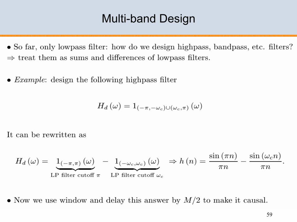
Multi-band Design

60
Frequency sampling method

61
FIR Filter Design Using Windows
FIR filter design based on windows is simple and robust, however, it is not optimal:• The resulting pass-band and stop-band parameters
are equal even though often the specification is more strict in the stop band than in the pass band
unnecessary high accuracy in the pass band
• The ripple of the window is not uniform (decays as we move away from discontinuity points according to side-lobe pattern of the window)
by allowing more freedom in the ripple behaviour we may be able to reduce filter’s order and hence its complexity

62
FIR Design by Optimisation: Least-Square Method
The integral of the weighted square frequency-domain error is given by
ε 2 = ∫E2(ω)dω
and we assume that the order and the type of the filter are known. Under this assumptions designing the FIR filter now reduces to determining the coefficients that would minimise ε 2 .
We now present a method that approximates the desired frequency response by a linear-phase FIRamplitude function according to the following optimality criterion.

63
Recall Our Example
ωp =0.2πωs =0.3πδ1 =0.1 δ2 =0.01
passband frequency
stopband frequency
But assume the pass-band tolerance of 0.1
Design a type I low-pass filter according to specification
The filter designed using window method cannot benefit from thisrelaxation, however, a least-square method design gives N = 33 (compared to N = 80).

64
Least-Square Design of FIR Filters
• Meeting the specification is not guaranteed a-priori, trial and error is often required. It might be useful to set the transition bands slightly narrower than needed, and it is often necessary to experiment with the weights
• Occasionally the resulting frequency response may be peculiar. Again, changing the weights would help to resolve the problem

65
Equiripple Design
The least-square criterion of minimising
is not entirely satisfactory.
A better approach is to minimize the maximum error at each band
ε 2 = ∫E2(ω)dω
ε = maxω |E(ω)|

66
Equiripple Design
The method is optimal in a sense of minimising the maximum magnitude of the ripple in all bands of interest, the filter order is fixed
It can be shown that this leads to an equiripple filter – a filter which amplitude response oscillates uniformly between the tolerance bounds of each band

67 67
-80
-60
-40
-20
0
0 1 2 3 4frequency (kHz)
resp
onse
(dB
)
-2
-1
0
1
2
0 1 2 3 4frequency (kHz)
resp
onse
(dB
)
Overall and passband-only frequency response of length 37 minimax filter
Many ripples achieve maximum Permitted amplitude
Passband
Equiripple Design

68
Remez method
• There exists a computational procedure known as the Remez method to solve this mathematical optimization problem.
• There are also exist formulae for estimating the required filter length in the case of lowpass, bandpass and narrow transition bandwidths. However, these formulae are not always reliable so it might be necessary to iterate the procedure so as to satisfy the design constraints.

69 69
The weights can be determined in advance from a minimax specification.
For example, if a simple lowpass filter has a requirement for the passbandgain to be in the range 1-∂p to 1+∂p, and the stopband gain to be less than ∂s, the weightings given to the passband and stopband errors would be ∂s and ∂p respectively.
The detailed algorithm is beyond the (time!) constraints of this module.
Equiripple Design: Weights
70
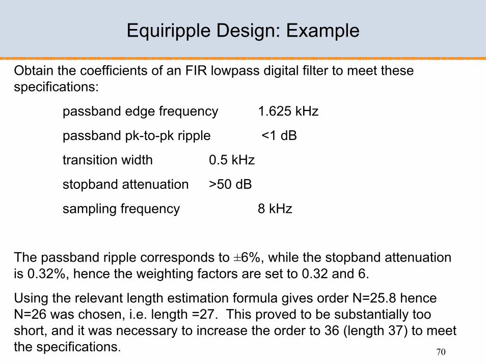
Obtain the coefficients of an FIR lowpass digital filter to meet these specifications:
passband edge frequency 1.625 kHz
passband pk-to-pk ripple <1 dB
transition width 0.5 kHz
stopband attenuation >50 dB
sampling frequency 8 kHz
The passband ripple corresponds to ±6%, while the stopband attenuation is 0.32%, hence the weighting factors are set to 0.32 and 6.
Using the relevant length estimation formula gives order N=25.8 hence N=26 was chosen, i.e. length =27. This proved to be substantially too short, and it was necessary to increase the order to 36 (length 37) to meet the specifications.
Equiripple Design: Example
71 71
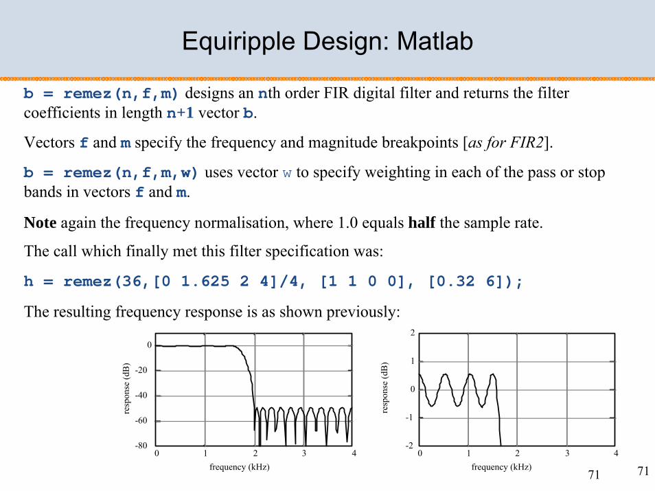
b = remez(n,f,m) designs an nth order FIR digital filter and returns the filter coefficients in length n+1 vector b.
Vectors f and m specify the frequency and magnitude breakpoints [as for FIR2].
b = remez(n,f,m,w) uses vector w to specify weighting in each of the pass or stop bands in vectors f and m.
Note again the frequency normalisation, where 1.0 equals half the sample rate.
The call which finally met this filter specification was:
h = remez(36,[0 1.625 2 4]/4, [1 1 0 0], [0.32 6]);
The resulting frequency response is as shown previously:
-80
-60
-40
-20
0
0 1 2 3 4frequency (kHz)
resp
onse
(dB
)
-2
-1
0
1
2
0 1 2 3 4frequency (kHz)
resp
onse
(dB
)
Equiripple Design: Matlab

72 72
The computational procedure the optimization problem is by Remez
The algorithm in common use is by Parks and McClellan.
The Parks-McClellan Remez exchange algorithm is widely available and versatile.
Important: it designs linear phase (symmetric) filters or antisymmetric filters of any of the standard types
The Parks-McClellan Remez exchange algorithm

73
The frequency response of the direct form FIR filter may be rearranged by grouping the terms involving the first and last coefficients, the second and next to last, etc.:
Linear Symmetric Filters
and then taking out a common factor exp( -jMΩ/2):
If the filter length M+1 is odd, then the final term in curly brackets above is the single term bM/2, that is the centre coefficient ('tap') of the filter.

74 74
Symmetric impulse response: if we put bM = b0, bM-1 = b1, etc., and note that exp(jθ)+exp(-jθ) = 2cos(θ), the frequency response becomes
This is a purely real function (sum of cosines) multiplied by a linear phase term, hence the response has linear phase, corresponding to a pure delay of M/2 samples, ie half the filter length.
A similar argument can be used to simplify antisymmetric impulse responses in terms of a sum of sine functions (such filters do not give a pure delay, although the phase still has a linear form π/2-mΩ/2)
Symmetric impulse response
75 75
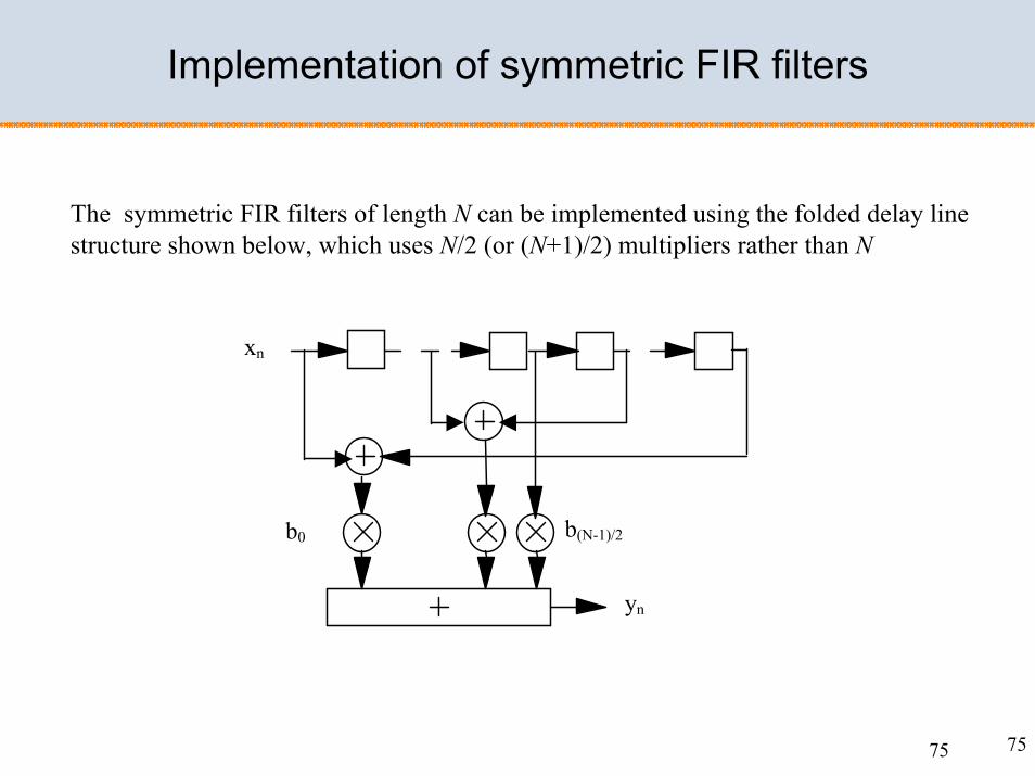
The symmetric FIR filters of length N can be implemented using the folded delay line structure shown below, which uses N/2 (or (N+1)/2) multipliers rather than N
xn
b0 b(N-1)/2
yn
Implementation of symmetric FIR filters

76 76
Linear phase in the stopbands is never a real requirement, and in some applications strictly linear phase in the passband is not needed either.
The linear phase filters designed by this method are therefore longer than optimum non-linear phase filters.
However, symmetric FIR filters of length N can be implemented using the folded delay line structure shown below, which uses N/2 (or (N+1)/2) multipliers rather than N, so the longer symmetric filter may be no more computationally intensive than a shorter non-linear phase one.
xn
b0 b(N-1)/2
yn
Limitations of the algorithm

77 77
More general non-linear optimisation (least squared error or minimax) can of course be used to design linear or non-linear phase FIR filters to meet more general frequency and/or time domain requirements.
Matlab has suitable optimisation routines.
Further options for FIR filter design

78
Thank you!