1

Part III. OFDM

Discrete Fourier Transform; Circular Convolution; Eigen Decomposition of Circulant Matrices

2

Motivation

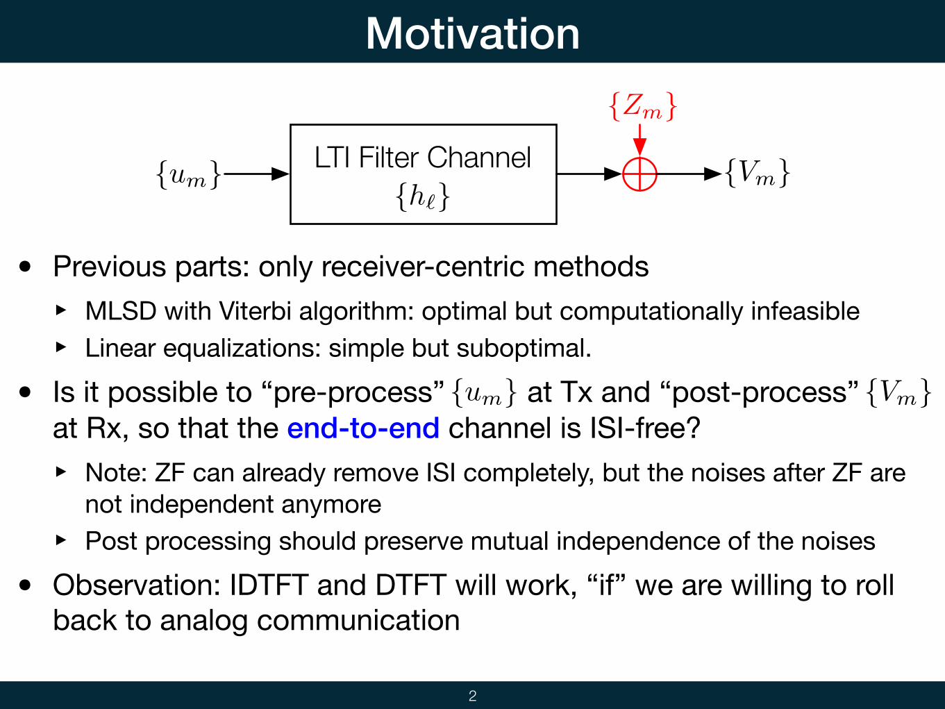
LTI Filter Channel{um} {Vm}{h`}

{Zm}

• Previous parts: only receiver-centric methods‣ MLSD with Viterbi algorithm: optimal but computationally infeasible‣ Linear equalizations: simple but suboptimal.

• Is it possible to “pre-process” at Tx and “post-process” at Rx, so that the end-to-end channel is ISI-free?‣ Note: ZF can already remove ISI completely, but the noises after ZF are

not independent anymore‣ Post processing should preserve mutual independence of the noises

• Observation: IDTFT and DTFT will work, “if” we are willing to roll back to analog communication

{um} {Vm}

3

{h`}

{Zm}

{um}

{Vm}

IDTFT

DTFT

u(f)

V (f)

um =

Z 1/2

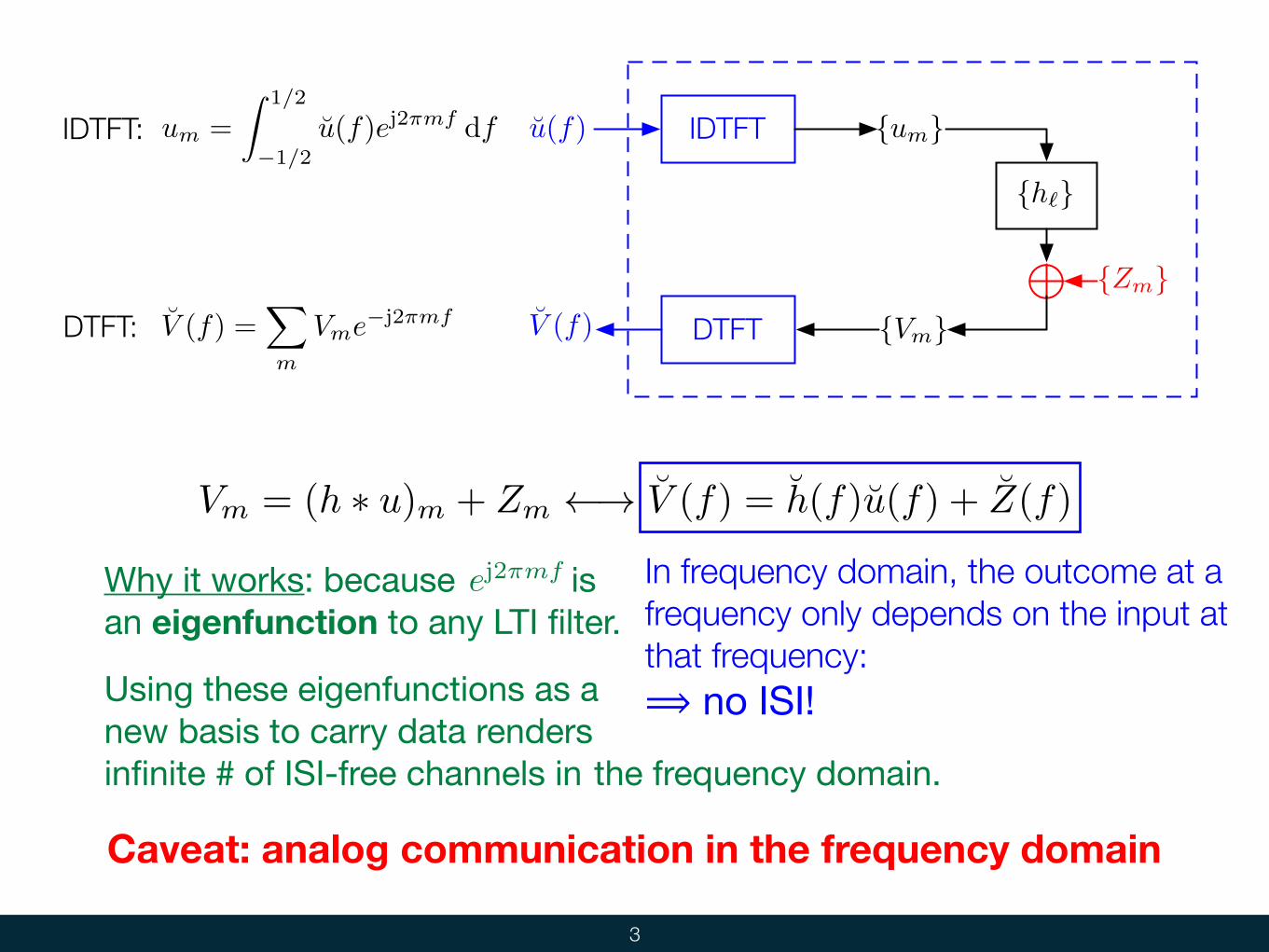
�1/2u(f)ej2⇡mf dfIDTFT:

DTFT: V (f) =X

m

Vme�j2⇡mf

Vm = (h ⇤ u)m + Zm ! V (f) = h(f)u(f) + Z(f)

In frequency domain, the outcome at a frequency only depends on the input at that frequency:⟹ no ISI!

Caveat: analog communication in the frequency domain

Why it works: because is an eigenfunction to any LTI filter.

ej2πmf

Using these eigenfunctions as a new basis to carry data renders infinite # of ISI-free channels in the frequency domain.

4

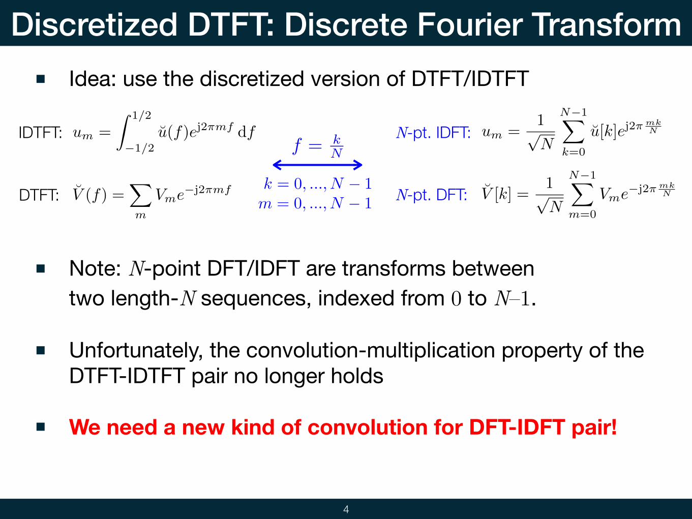
Discretized DTFT: Discrete Fourier TransformIdea: use the discretized version of DTFT/IDTFT

um =

Z 1/2

�1/2u(f)ej2⇡mf dfIDTFT:

DTFT: V (f) =X

m

Vme�j2⇡mf

N-pt. IDFT:

N-pt. DFT:

um =1pN

N�1X

k=0

u[k]ej2⇡mkN

V [k] =1pN

N�1X

m=0

Vme�j2⇡mkN

f = kN

k = 0, ..., N − 1m = 0, ..., N − 1

Note: N-point DFT/IDFT are transforms between two length-N sequences, indexed from 0 to N–1.

Unfortunately, the convolution-multiplication property of the DTFT-IDTFT pair no longer holds

We need a new kind of convolution for DFT-IDFT pair!

Circular Convolution

5

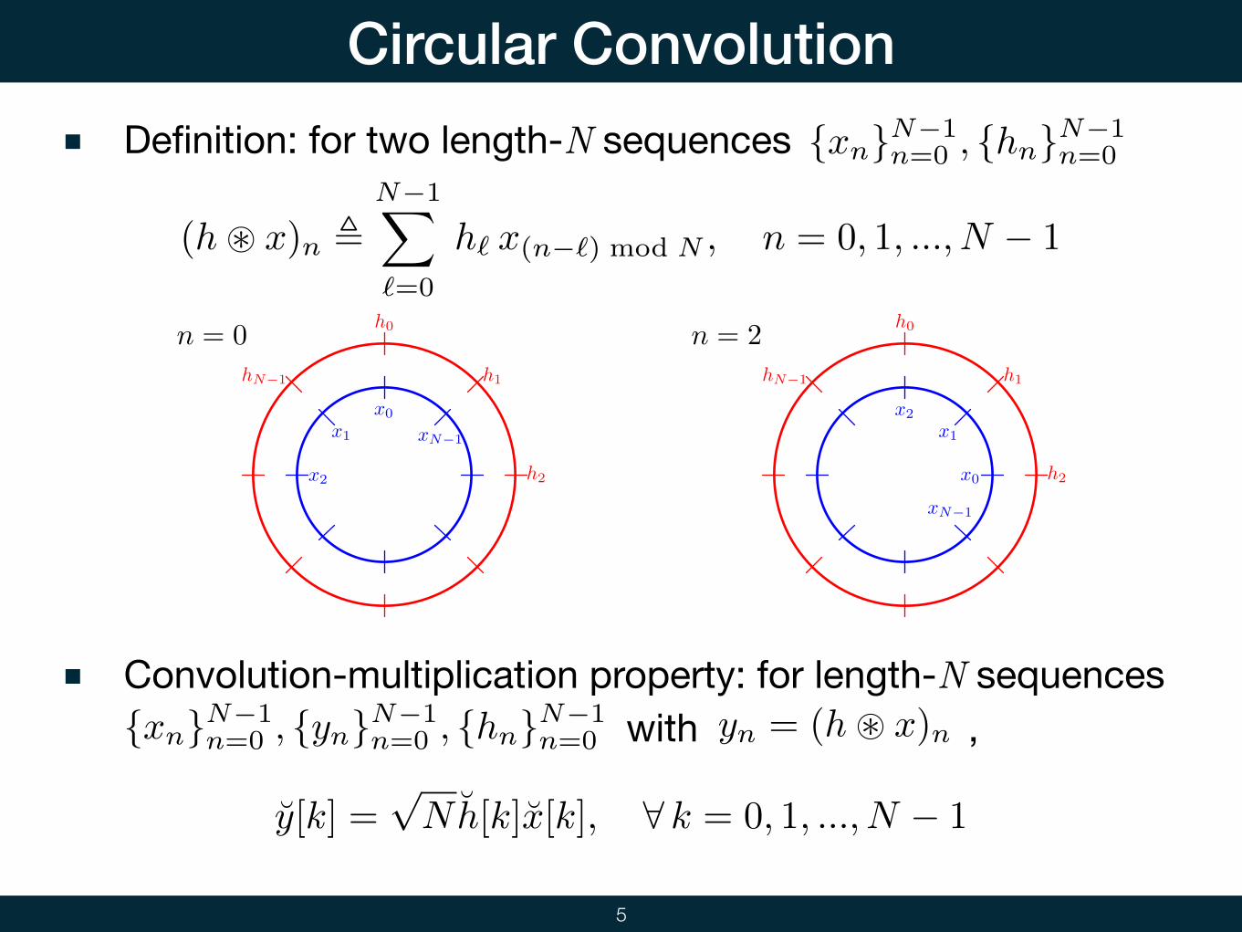
Definition: for two length-N sequences

Convolution-multiplication property: for length-N sequences with , {xn}N−1

n=0 , {yn}N−1n=0 , {hn}N−1

n=0 yn = (h~ x)n

y[k] =pNh[k]x[k], 8 k = 0, 1, ..., N � 1

{xn}N−1n=0 , {hn}N−1

n=0

(h~ x)n ,N�1X

`=0

h` x(n�`) mod N , n = 0, 1, ..., N � 1

h0

h1

h2

hN�1

xN�1

x0

x1

x2

n = 0h0

h1

h2

hN�1

xN�1

x0

x1

x2

n = 2

h0 h1 hL�1· · ·

u0uN�1 · · · · · ·uN�L+1

uN�1 · · · uN�L+1

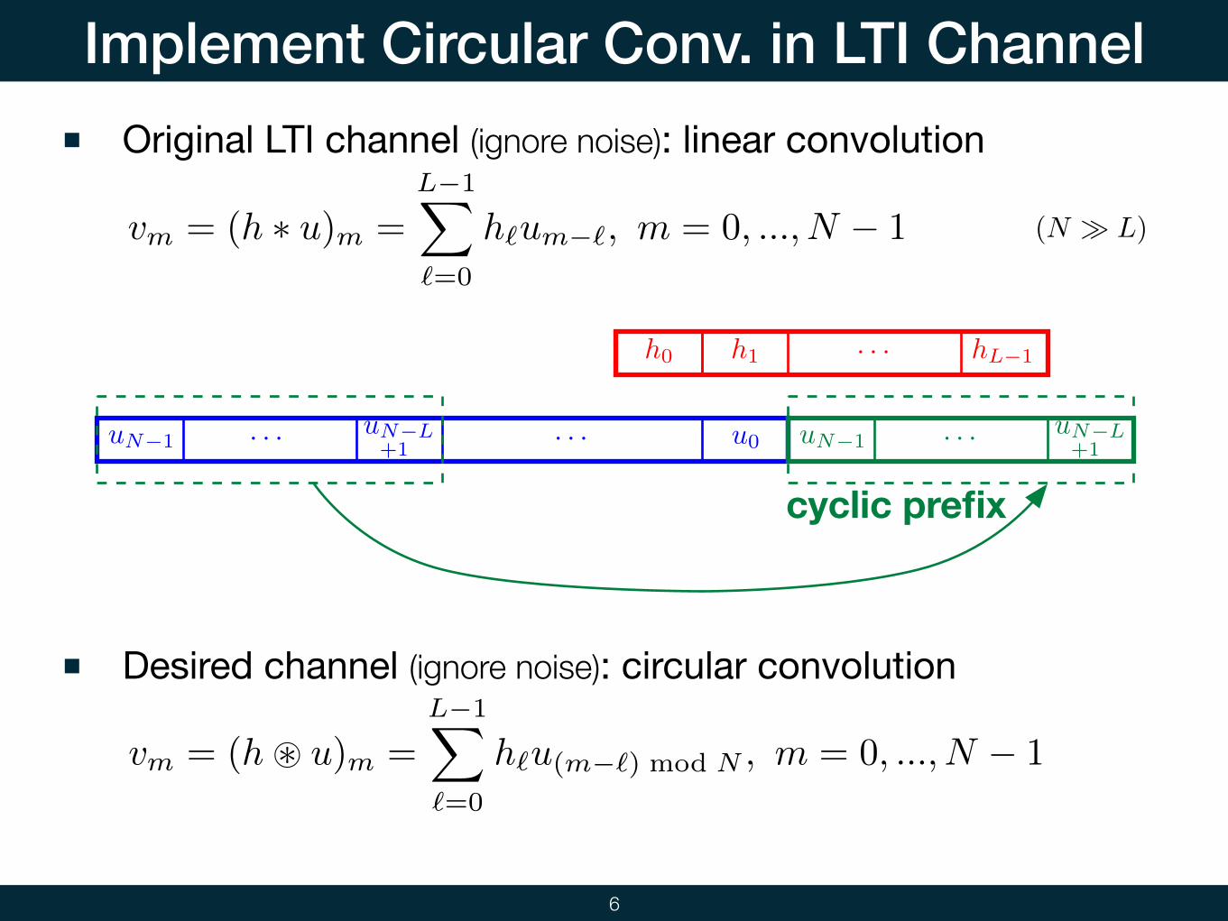
Implement Circular Conv. in LTI Channel

6

Original LTI channel (ignore noise): linear convolution

(N � L)vm = (h ⇤ u)m =L�1X

`=0

h`um�`, m = 0, ..., N � 1

Desired channel (ignore noise): circular convolution

vm = (h~ u)m =L�1X

`=0

h`u(m�`) mod N , m = 0, ..., N � 1

cyclic prefix

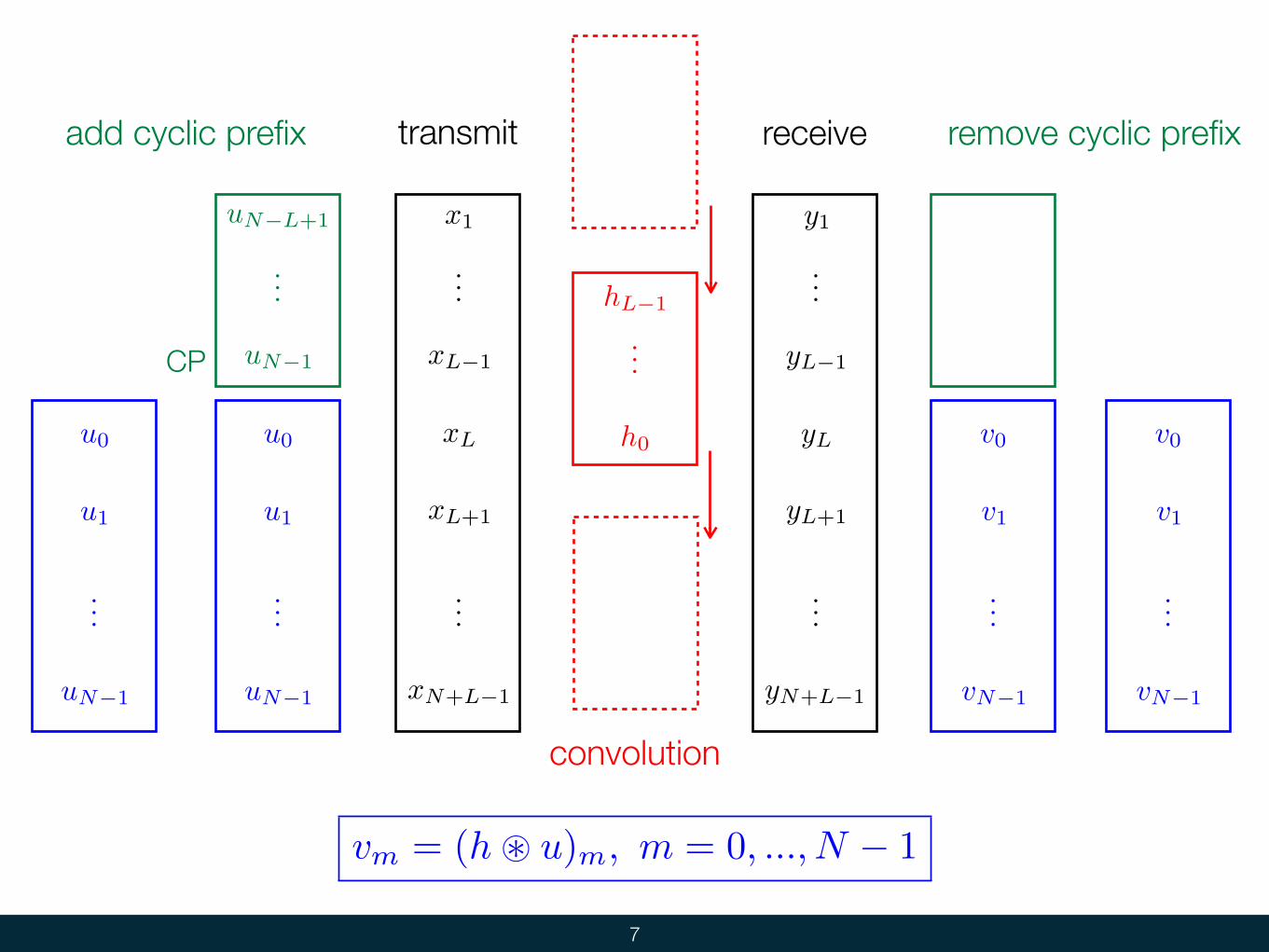
7

transmit

uN�L+1

uN�1

u0

u1

uN�1

u0

u1

uN�1

CP

x1

xL�1

xL

xN+L�1

xL+1

add cyclic prefix

convolution

receive

y1

yL�1

yL

yL+1

yN+L�1 vN�1

v1

v0

remove cyclic prefix

vN�1

v1

v0

vm = (h~ u)m, m = 0, ..., N � 1

h0

hL�1

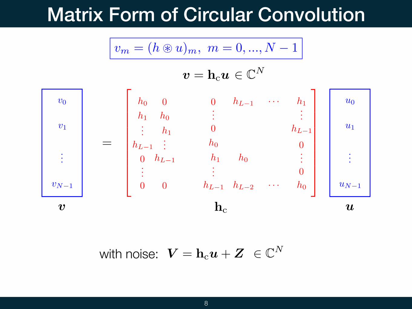
Matrix Form of Circular Convolution

8

u0

u1

uN�1vN�1

v1

v0

=

vm = (h~ u)m, m = 0, ..., N � 1

v u

3

777777775

2

666666664

h0

h1

hL�1

0

0

0

h0

h1

hL�1

0

h0

h1

hL�1

0

0

hL�1 h1· · ·

h0

hL�2 h0· · ·

0

0

hL�1

hc

v = hcu

V = hcu+Zwith noise: ∈ CN

∈ CN

Linear Algebraic View

9

3

777777775

2

666666664

h0

h1

hL�1

0

0

0

h0

h1

hL�1

0

h0

h1

hL�1

0

0

hL�1 h1· · ·

h0

hL�2 h0· · ·

0

0

hL�1

hc

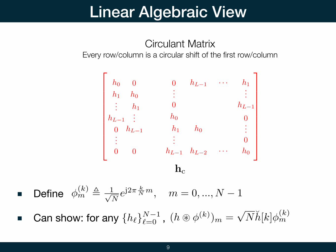
Circulant MatrixEvery row/column is a circular shift of the first row/column

Define

Can show: for any , {hℓ}N−1ℓ=0

φ(k)m ! 1√

Nej2π

kN m, m = 0, ..., N − 1

(h! φ(k))m =√Nh[k]φ(k)

m

10

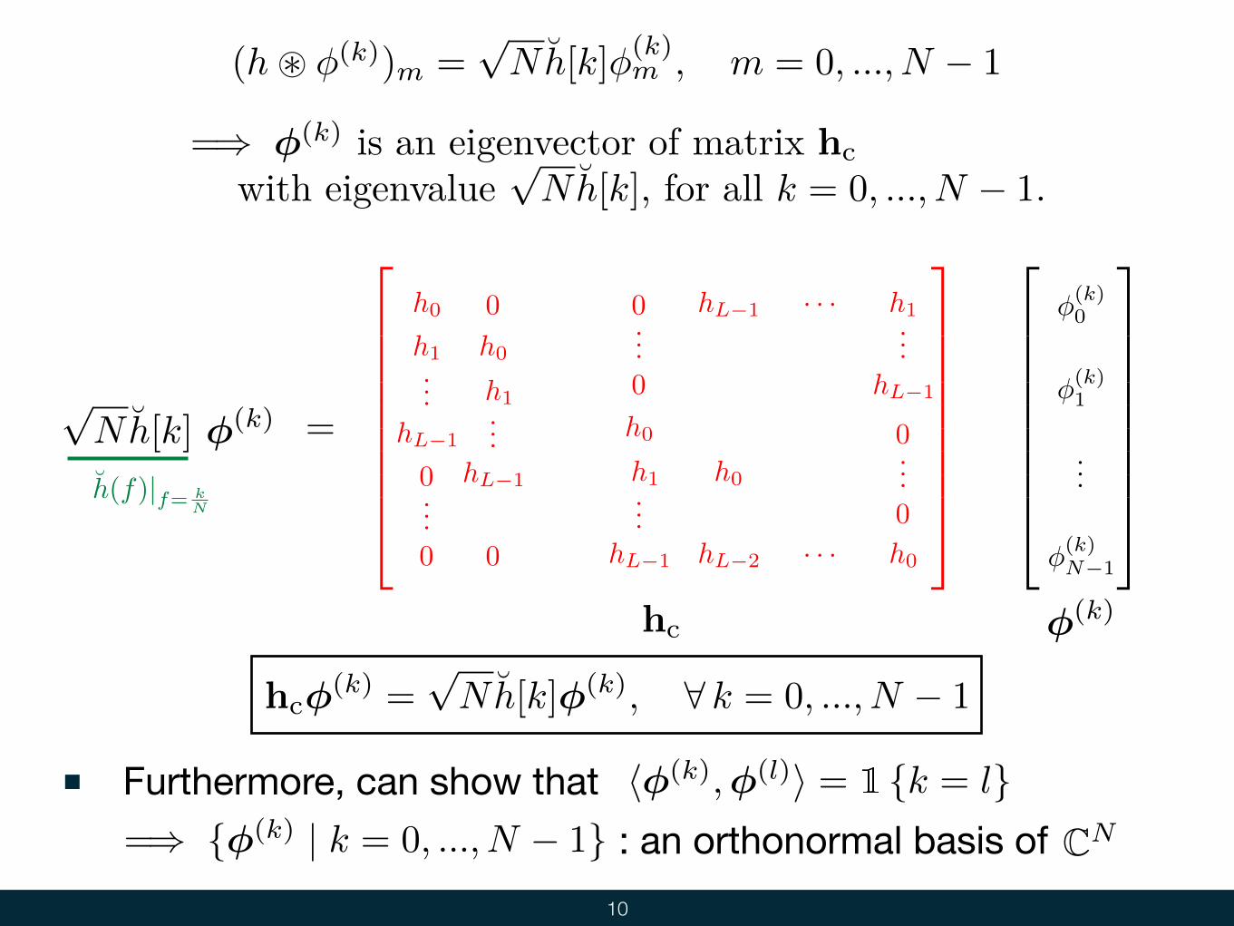
(h! φ(k))m =√Nh[k]φ(k)

m , m = 0, ..., N − 1

=) �(k) hcpNh[k] k = 0, ..., N � 1

3

777777775

2

666666664

h0

h1

hL�1

0

0

0

h0

h1

hL�1

0

h0

h1

hL�1

0

0

hL�1 h1· · ·

h0

hL�2 h0· · ·

0

0

hL�1

hc

=�(k)

2

666666664

3

777777775

�(k)0

�(k)1

�(k)N�1

�(k)

pNh[k]

h(f)|f= kN

hc�(k) =

pNh[k]�(k), 8 k = 0, ..., N � 1

Furthermore, can show that ⟨φ(k),φ(l)⟩ = {k = l}=) {�(k) | k = 0, ..., N � 1} CN: an orthonormal basis of

11

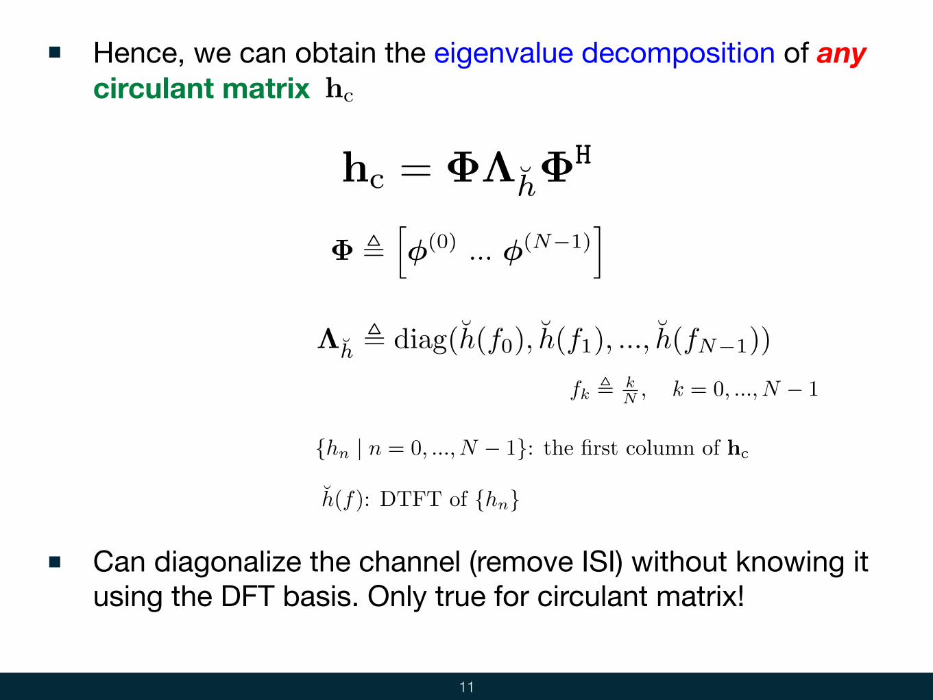
Hence, we can obtain the eigenvalue decomposition of any circulant matrix hc

hc = ΦΛhΦH

Φ !!φ(0) ... φ(N−1)

"

Λh ! diag(h(f0), h(f1), ..., h(fN−1))

fk ! kN , k = 0, ..., N − 1

{hn | n = 0, ..., N � 1} hc

h(f) {hn}

Can diagonalize the channel (remove ISI) without knowing it using the DFT basis. Only true for circulant matrix!

12

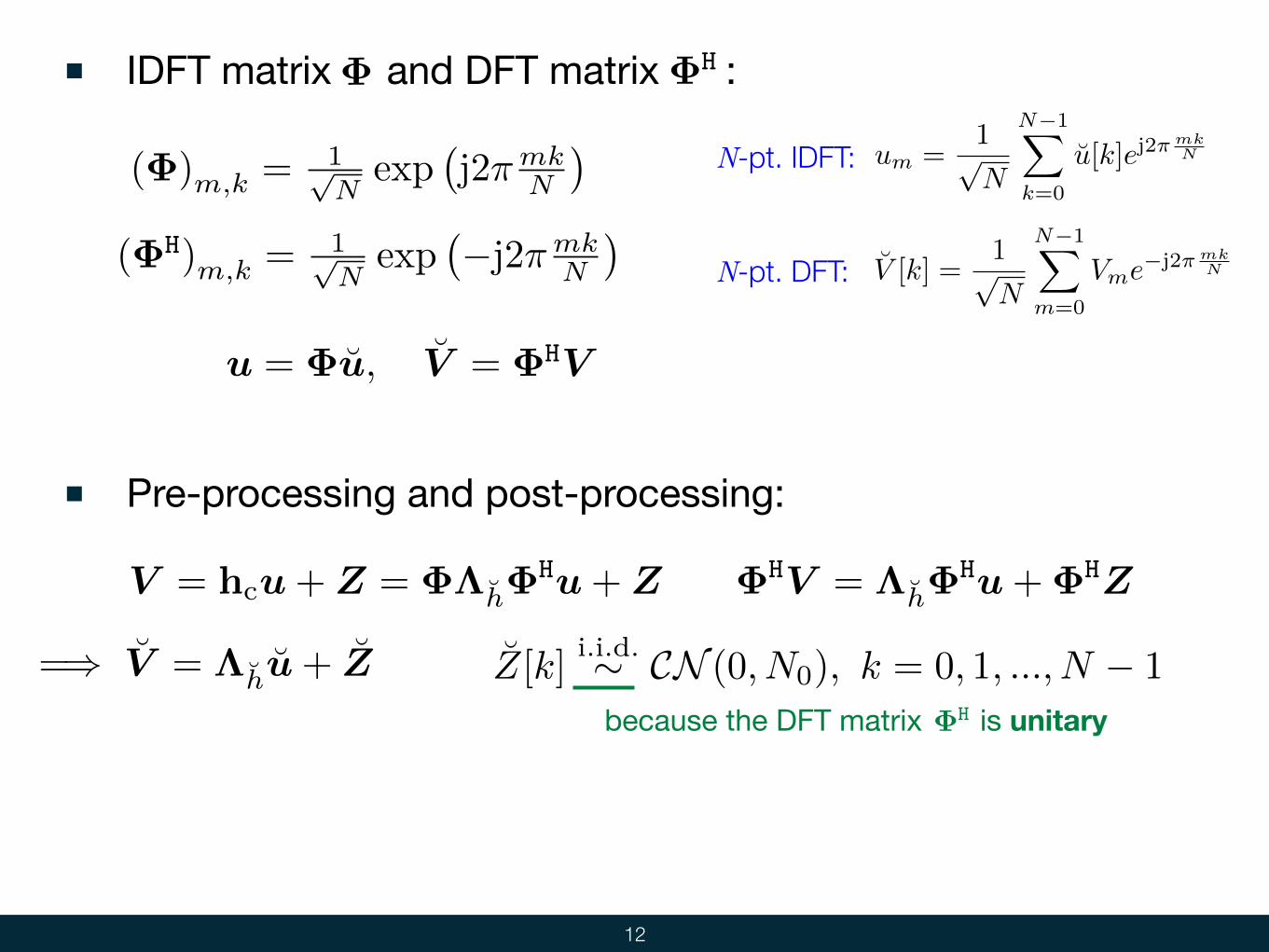
(Φ)m,k = 1√Nexp

!j2πmk

N

"IDFT matrix and DFT matrix : Φ

(ΦH)m,k = 1√Nexp

!−j2πmk

N

"

ΦH

N-pt. IDFT:

N-pt. DFT:

um =1pN

N�1X

k=0

u[k]ej2⇡mkN

V [k] =1pN

N�1X

m=0

Vme�j2⇡mkN

u = Φu, V = ΦHV

V = hcu+Z = �⇤h�Hu+Z �HV = ⇤h�

Hu+�HZ

Pre-processing and post-processing:

=) V = ⇤hu+ Z Z[k] ⇠ CN (0, N0), k = 0, 1, ..., N � 1because the DFT matrix is unitary ΦH

Equivalent Parallel Channels

13

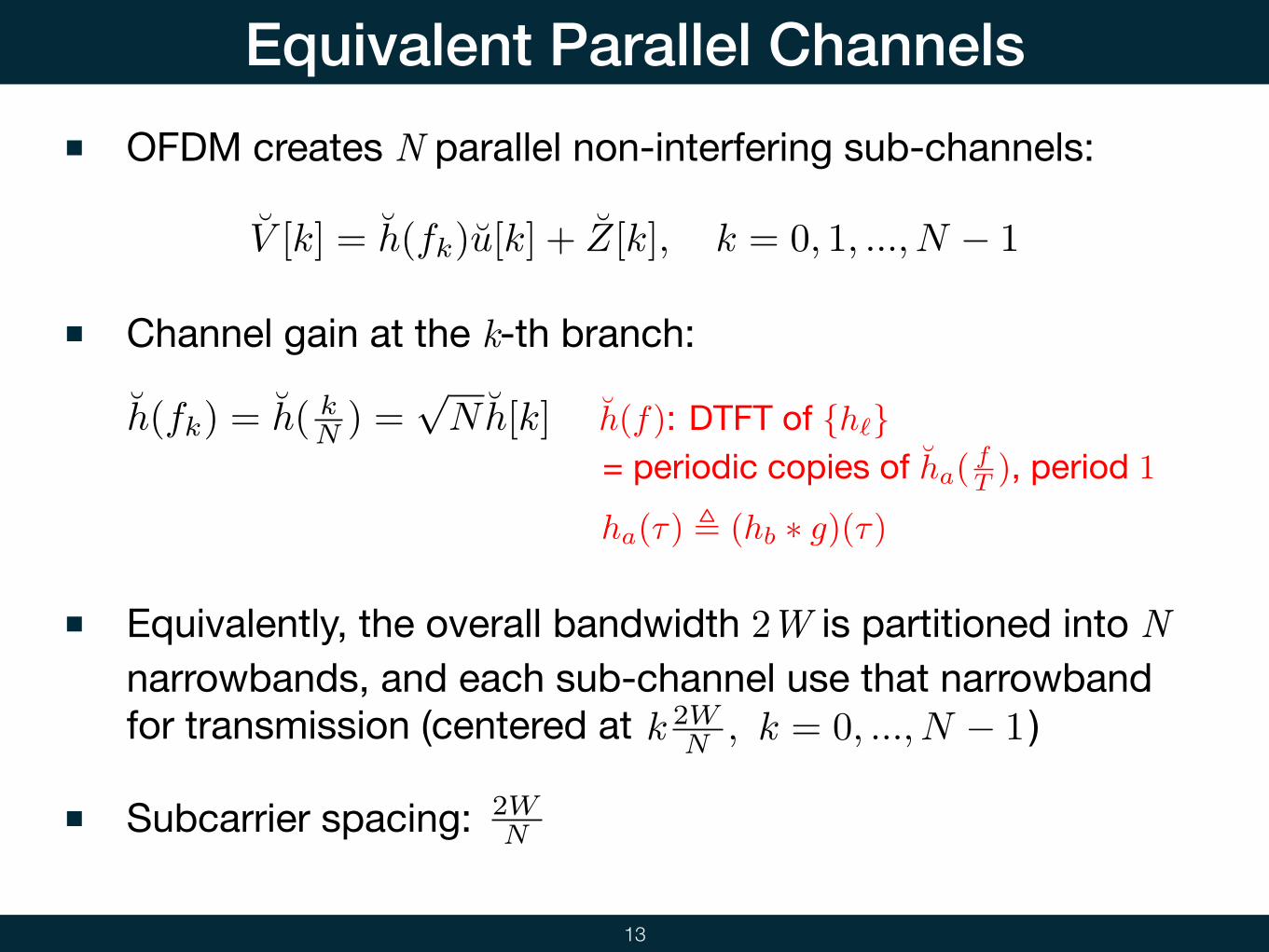
OFDM creates N parallel non-interfering sub-channels:

V [k] = h(fk)u[k] + Z[k], k = 0, 1, ..., N − 1

Channel gain at the k-th branch:

h(fk) = h( kN ) =

√Nh[k] h(f): DTFT of {h`}

= periodic copies of ha(fT ), period 1

ha(τ) ! (hb ∗ g)(τ)

Equivalently, the overall bandwidth 2W is partitioned into N narrowbands, and each sub-channel use that narrowband for transmission (centered at ) k 2W

N , k = 0, ..., N − 1

Subcarrier spacing: 2WN

Capacity of Parallel Channels

14

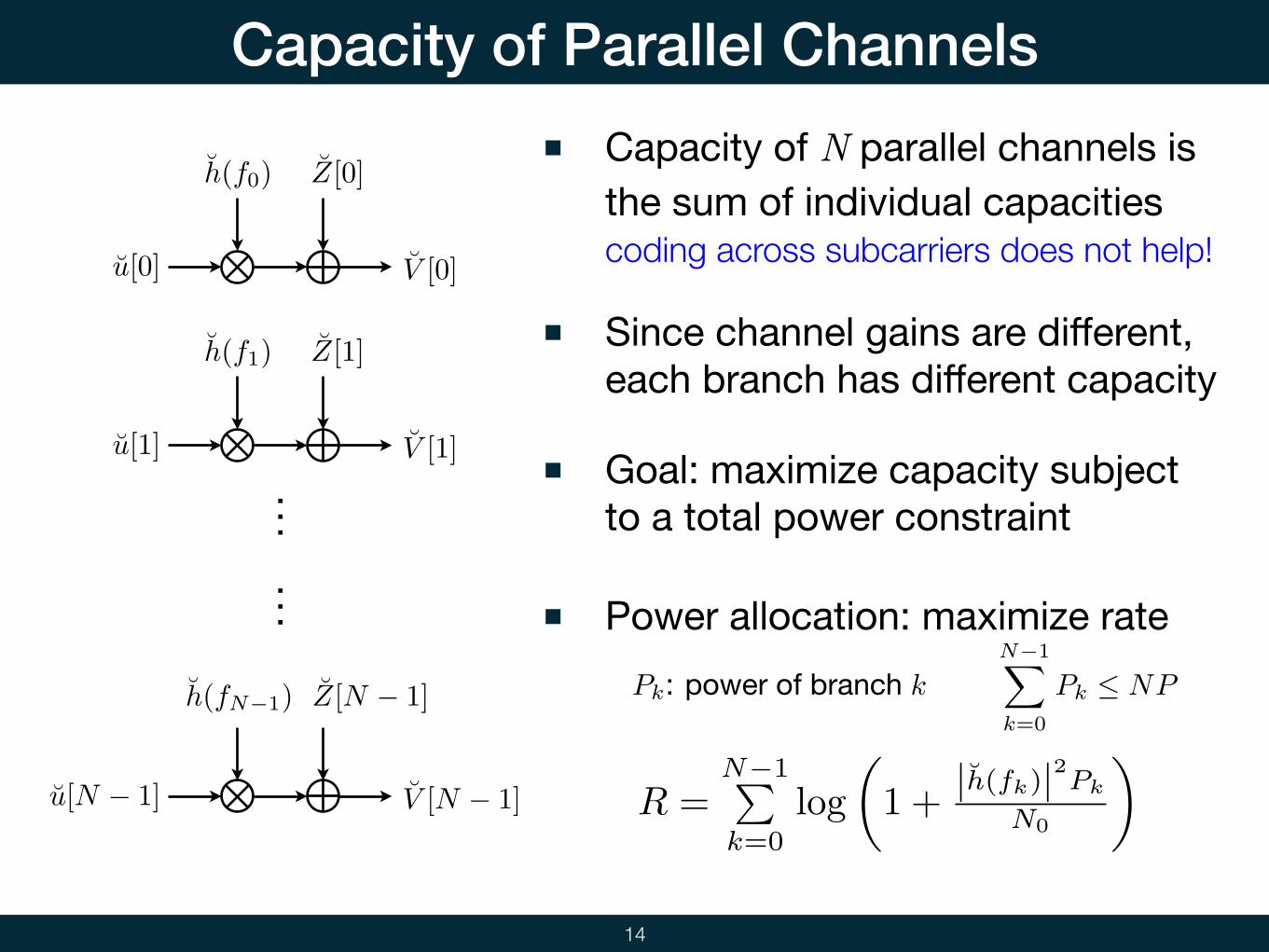
h(f0)

u[0] V [0]

Z[0]

u[1]

h(f1) Z[1]

V [1]

u[N − 1]

h(fN−1) Z[N − 1]

V [N − 1]

...

...

Capacity of N parallel channels is the sum of individual capacities

Since channel gains are different, each branch has different capacity

coding across subcarriers does not help!

Goal: maximize capacity subject to a total power constraint

Power allocation: maximize ratePk: power of branch k

N�1X

k=0

Pk NP

R =N−1!k=0

log

"1 +

|h(fk)|2Pk

N0

#

Water-filling

15

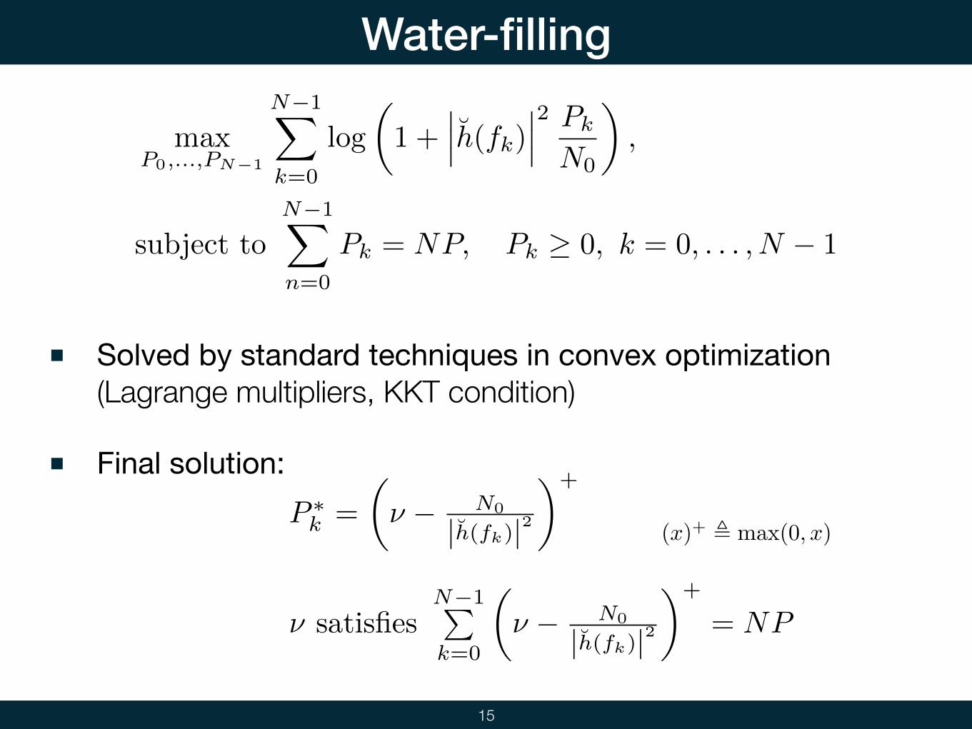
max

P0,...,PN�1

N�1X

k=0

log

✓1 +

���˘h(fk)���2 Pk

N0

◆,

N�1X

n=0

Pk = NP, Pk � 0, k = 0, . . . , N � 1

Solved by standard techniques in convex optimization (Lagrange multipliers, KKT condition)

Final solution:P ∗k =

!ν − N0

|h(fk)|2"+

νN−1!k=0

"ν − N0

|h(fk)|2#+

= NP

(x)+ ! max(0, x)

16

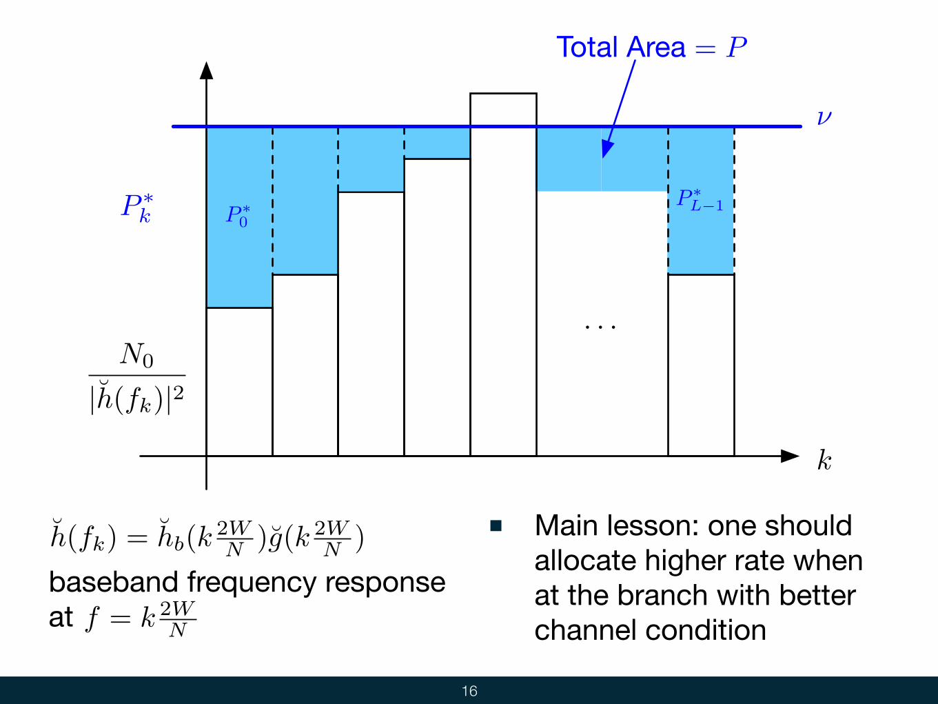
h(fk) = hb(k2WN )g(k 2W

N )

baseband frequency response at f = k 2W

N

Main lesson: one should allocate higher rate when at the branch with better channel condition

N0

|h(fk)|2

k

⌫

Total Area = P

· · ·

P ⇤k P ⇤

0

P ⇤L�1

17

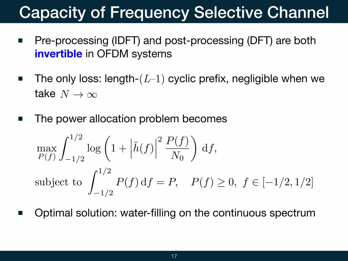
Capacity of Frequency Selective ChannelPre-processing (IDFT) and post-processing (DFT) are both invertible in OFDM systems

The only loss: length-(L–1) cyclic prefix, negligible when we take N → ∞

The power allocation problem becomes

Optimal solution: water-filling on the continuous spectrum

max

P (f)

Z 1/2

�1/2log

✓1 +

���˘h(f)���2 P (f)

N0

◆df,

Z 1/2

�1/2P (f) df = P, P (f) � 0, f 2 [�1/2, 1/2]

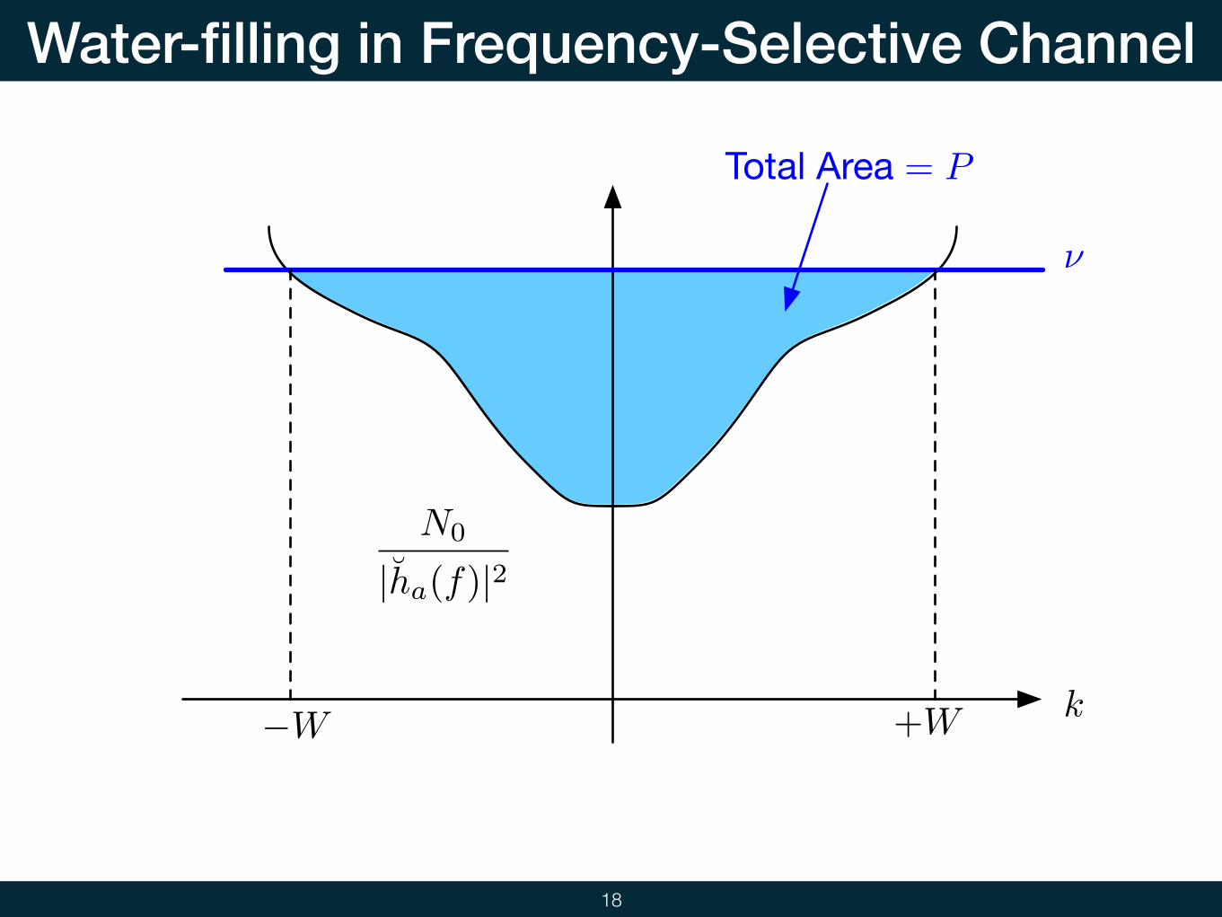
Water-filling in Frequency-Selective Channel

18

k

N0

|ha(f)|2

⌫

Total Area = P

�W +W

19

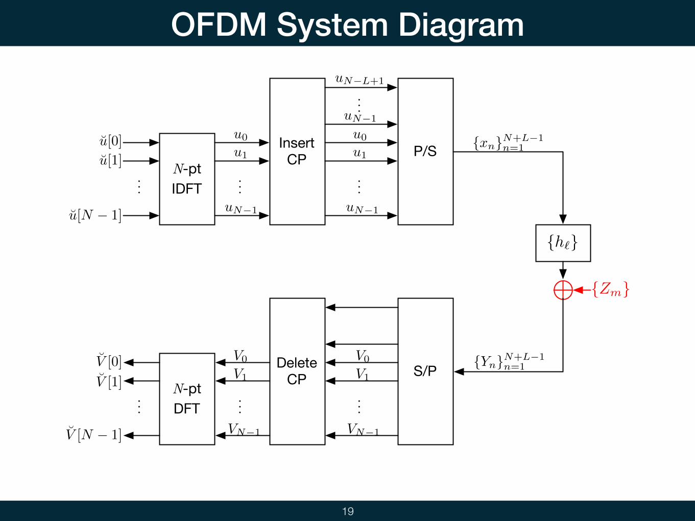
OFDM System Diagram

N-ptIDFT

u[0]

u[1]

u[N � 1]

u0

u1

uN�1

Insert CP

uN�L+1

uN�1

u0

u1

uN�1

P/S {xn}N+L�1n=1

{h`}

{Zm}

S/PDelete CP

{Yn}N+L�1n=1

V0

V1

VN�1

V0

V1

VN�1

N-ptDFT

V [N � 1]

V [0]

V [1]

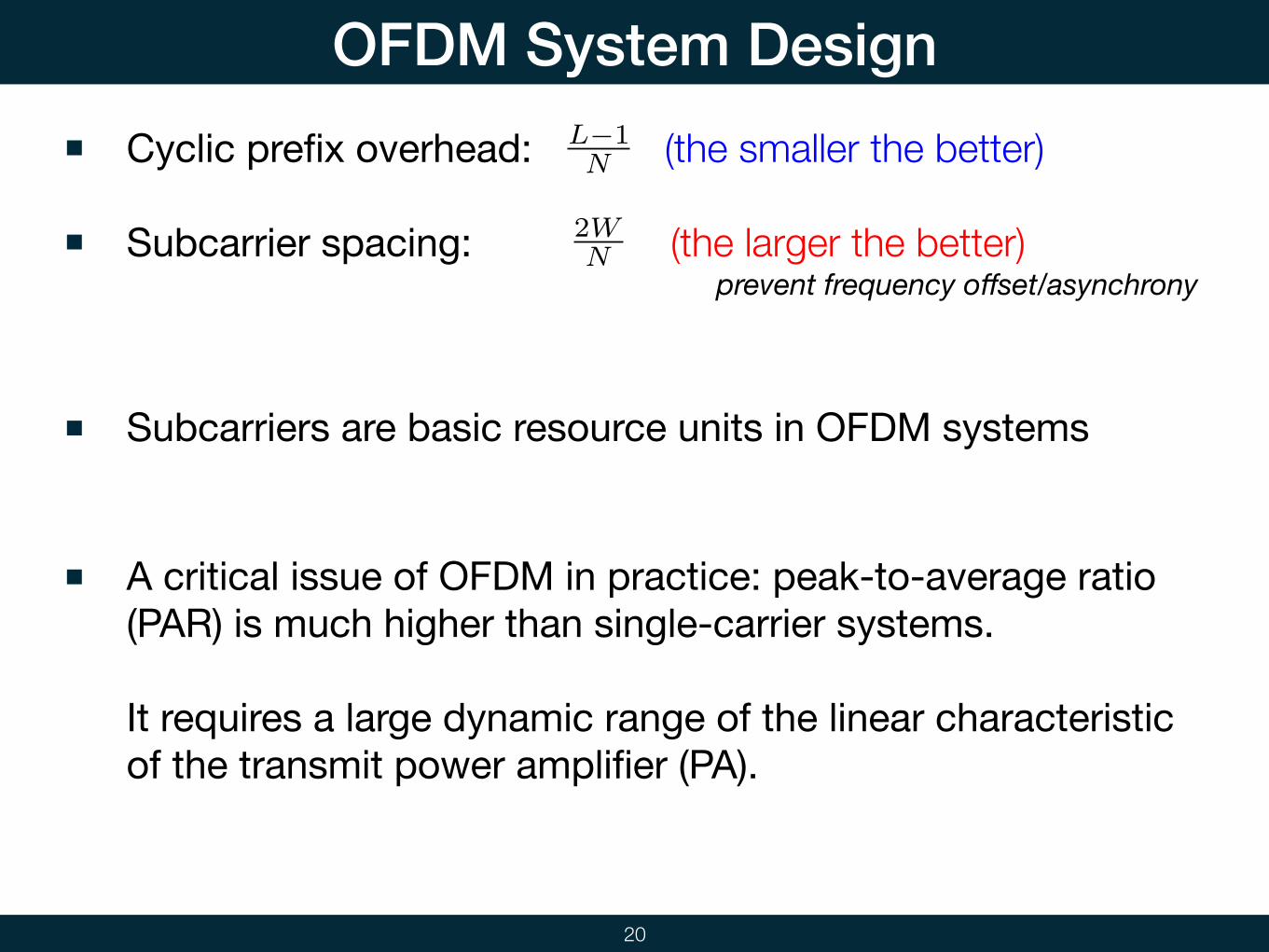
OFDM System Design

20

Cyclic prefix overhead: (the smaller the better) L−1N

Subcarrier spacing: (the larger the better)prevent frequency offset/asynchrony

2WN

Subcarriers are basic resource units in OFDM systems

A critical issue of OFDM in practice: peak-to-average ratio (PAR) is much higher than single-carrier systems.

It requires a large dynamic range of the linear characteristic of the transmit power amplifier (PA).