half-delocalization of eigenfunctions for the …irma.math.unistra.fr/~anantharaman/lap12.pdf ·...

HALF-DELOCALIZATION OF EIGENFUNCTIONS FOR THELAPLACIAN ON AN ANOSOV MANIFOLD

NALINI ANANTHARAMAN AND STÉPHANE NONNENMACHER

Abstract. We study the high-energy eigenfunctions of the Laplacian on a compact Rie-mannian manifold with Anosov geodesic flow. The localization of a semiclassical measureassociated with a sequence of eigenfunctions is characterized by the Kolmogorov-Sinaientropy of this measure. We show that this entropy is necessarily bounded from belowby a constant which, in the case of constant negative curvature, equals half the maximalentropy. In this sense, high-energy eigenfunctions are at least half-delocalized.

The theory of quantum chaos tries to understand how the chaotic behaviour of a clas-sical Hamiltonian system is reflected in its quantum version. For instance, let M be acompact Riemannian C∞ manifold, such that the geodesic flow has the Anosov property— the ideal chaotic behaviour. The corresponding quantum dynamics is the unitary flowgenerated by the Laplace-Beltrami operator on L2(M). One expects that the chaoticproperties of the geodesic flow influence the spectral theory of the Laplacian. The RandomMatrix conjecture [6] asserts that the high-lying eigenvalues should, after proper renormal-ization, statistically resemble those of a large random matrix, at least for a generic Anosovmetric. The Quantum Unique Ergodicity conjecture [27] (see also [5, 30]) deals with thecorresponding eigenfunctions ψ: it claims that the probability density |ψ(x)|2dx shouldapproach (in a weak sense) the Riemannian volume, when the eigenvalue correspondingto ψ tends to infinity. In fact a stronger property should hold for the Wigner transformWψ, a distribution on the cotangent bundle T ∗M which describes the distribution of thewave function ψ on the phase space T ∗M . We will adopt a semiclassical point of view,that is consider the eigenstates of eigenvalue unity of the semiclassical Laplacian −~24, inthe semiclassical limit ~→ 0. Weak limits of the distributions Wψ are called semiclassicalmeasures: they are invariant measures of the geodesic flow on the unit energy layer E . TheQuantum Unique Ergodicity conjecture asserts that on an Anosov manifold there exists aunique semiclassical measure, namely the Liouville measure on E ; in other words, in thesemiclassical régime all eigenfunctions become uniformly distributed over E .

For manifolds with an ergodic geodesic flow (with respect to the Liouville measure), it hasbeen shown by Schnirelman, Zelditch and Colin de Verdière that almost all eigenfunctionsbecome uniformly distributed over E , in the semiclassical limit: this property is dubbed asQuantum Ergodicity [28, 32, 8]. The possibility of exceptional sequences of eigenstates withdifferent semiclassical limits remains open in general. The Quantum Unique Ergodicityconjecture states that such sequences do not exist for an Anosov manifold [27].

1

2 N. ANANTHARAMAN AND S. NONNENMACHER

So far the most precise results on this question were obtained for Anosov manifoldsM with arithmetic properties: see Rudnick–Sarnak [27], Wolpert [31]. Recently, Linden-strauss [24] proved the asymptotic equidistribution of all “arithmetic” eigenstates (theseare believed to exhaust the full family of eigenstates). The proof, unfortunately, cannot beextended to general Anosov manifolds.

To motivate the conjecture, one may instead invoke the following dynamical explanation.By the Heisenberg uncertainty principle, an eigenfunction cannot be strictly localized ona submanifold in phase space. Its microlocal support must contain a symplectic cubeof volume ~d, where d is the dimension of M . Since ψ is invariant under the quantumdynamics, which is semiclassically approximated by the geodesic flow, the fast mixingproperty of the latter will spread this cube throughout the energy layer, showing that thesupport of the eigenfunction must also spread throughout E .

This argument is however too simplistic. First, Colin de Verdière and Parisse showedthat, on a surface of revolution of negative curvature, eigenfunctions can concentrate ona single periodic orbit in the semiclassical limit, despite the exponential unstability ofthat orbit [9]. Their construction shows that one cannot use purely local features, suchas instability, to rule out localization of eigenfunctions on closed geodesics. Second, theargument above is based on the classical dynamics, and does not take into account theinterferences of the wavefunction with itself, after a long time. Faure, Nonnenmacher andDe Bièvre exhibited in [14] a simple example of a symplectic Anosov dynamical system,namely the action of a linear hyperbolic automorphism on the 2-torus (also called “Arnold’scat map”), the quantization of which does not satisfy the Quantum Unique Ergodicityconjecture. Precisely, they construct a family of eigenstates for which the semiclassicalmeasure consists in two ergodic components: half of it is the Liouville measure, while theother half is a Dirac peak on a single unstable periodic orbit. It was also shown that —in the case of the “cat map” — this half-localization on a periodic orbit is maximal [15].Another type of semiclassical measures was recently exhibited by Kelmer for quantizedautomorphisms on higher-dimensional tori and some of their perturbations [19, 20]: itconsists in the Lebesgue measure on some invariant co-isotropic subspace of the torus. Inthose cases, the existence of exceptional eigenstates is due to some nongeneric algebraicproperties of the classical and quantized systems.

In a previous paper [2], we discovered how to use an information-theoretic variant ofthe uncertainty principle [22, 25], called the Entropic Uncertainty Principle, to constrainthe localization properties of eigenfunctions in the case of another toy model, the Walsh-quantized baker’s map. For any dynamical system, the complexity of an invariant measurecan be described through its Kolmogorov–Sinai entropy. In the case of the Walsh-baker’smap, we showed that the entropy of semiclassical measures must be at least half the entropyof the Lebesgue measure. Thus, our result can be interpreted as a “half-delocalization” ofeigenstates. The Walsh-baker model being very special, it was not clear whether thestrategy could be generalized to more realistic systems, like geodesic flows or more generalsymplectic systems quantized à la Weyl.

HALF-DELOCALIZATION 3

In this paper we show that it is the case: the strategy used in [2] is rather general,and its implementation to the case of Anosov geodesic flows only requires more technicalsuffering.

1. Main result.

Let M be a compact Riemannian manifold. We will denote by |·|x the norm on T ∗xMgiven by the metric. The geodesic flow (gt)t∈R is the Hamiltonian flow on T ∗M generatedby the Hamiltonian

H(x, ξ) =|ξ|2x2.

In the semiclassical setting, the corresponding quantum operator is −~242, which generates

the unitary flow (U t) = (exp(it~42)) acting on L2(M).

We denote by (ψk)k∈N an orthonormal basis of L2(M) made of eigenfunctions of theLaplacian, and by ( 1

~2k)k∈N the corresponding eigenvalues:

−~2k4ψk = ψk, with ~k+1 ≤ ~k .

We are interested in the high-energy eigenfunctions of −4, in other words the semiclassicallimit ~k → 0.

The Wigner distribution associated to an eigenfunction ψk is defined by

Wk(a) = 〈Op~k(a)ψk, ψk〉L2(M), a ∈ C∞c (T ∗M) .

Here Op~kis a quantization procedure, set at the scale ~k, which associates a bounded oper-

ator on L2(M) to any smooth phase space function a with nice behaviour at infinity (see forinstance [10]). If a is a function on the manifold M , we have Wk(a) =

∫Ma(x)|ψk(x)|2dx:

the distribution Wk is a microlocal lift of the probability measure |ψk(x)|2dx into a phasespace distribution. Although the definition of Wk depends on a certain number of choices,like the choice of local coordinates, or of the quantization procedure (Weyl, anti-Wick,“right” or “left” quantization...), its asymptotic behaviour when ~k −→ 0 does not. Ac-cordingly, we call semiclassical measures the limit points of the sequence (Wk)k∈N, in thedistribution topology.

Using standard semiclassical arguments, one easily shows the following [8]:

Proposition 1.1. Any semiclassical measure is a probability measure carried on the energylayer E = H−1(1

2) (which coincides with the unit cotangent bundle E = S∗M). This measure

is invariant under the geodesic flow.

If the geodesic flow has the Anosov property — for instance if M has negative sectionalcurvature — then there exist many invariant probability measures on E , in addition to theLiouville measure. The geodesic flow has countably many periodic orbits, each of themcarrying an invariant probability measure. There are still many others, like the equilibriumstates obtained by variational principles [18]. The Kolmogorov–Sinai entropy, also calledmetric entropy, of a (gt)-invariant probability measure µ is a nonnegative number hKS(µ)that describes, in some sense, the complexity of a µ-typical orbit of the flow. For instance,


a measure carried on a closed geodesic has zero entropy. An upper bound on the entropy isgiven by the Ruelle inequality: since the geodesic flow has the Anosov property, the energylayer E is foliated into unstable manifolds of the flow, and for any invariant probabilitymeasure µ one has

(1.1) hKS(µ) ≤∣∣∣∣∫

Elog Ju(ρ)dµ(ρ)

∣∣∣∣ .

In this inequality, Ju(ρ) is the unstable Jacobian of the flow at the point ρ ∈ E , defined asthe Jacobian of the map g−1 restricted to the unstable manifold at the point g1ρ. Althoughlog Ju(ρ) depends on the metric structure on E , its average over any invariant measure doesnot, and this average is always negative. If M has dimension d and has constant sectionalcurvature −1, this inequality just reads hKS(µ) ≤ d− 1. The equality holds in (1.1) if andonly if µ is the Liouville measure on E [23]. Our central result is the following

Theorem 1.2. Let M be a compact smooth Riemannian manifold with Anosov geodesicflow. Let µ be a semiclassical measure associated to the eigenfunctions of the Laplacian onM . Then the metric entropy of µ with respect to the geodesic flow satisfies

(1.2) hKS(µ) ≥ 3

2

∣∣∣∣∫

Elog Ju(ρ)dµ(ρ)

∣∣∣∣− (d− 1)λmax ,

where d = dimM and λmax = limt→±∞ 1tlog supρ∈E |dgtρ| is the maximal expansion rate of

the geodesic flow on E.In particular, if M has constant sectional curvature −1, this means that

(1.3) hKS(µ) ≥ d− 1

2.

The first author proved in [1] that the entropy of such a semiclassical measure is boundedfrom below by a positive (hardly explicit) constant. The bound (1.3) in the above theoremis much sharper in the case of constant curvature. On the other hand, if the curvaturevaries a lot (still being negative everywhere), the right hand side of (1.2) may actuallybe negative, in which case the above bound is trivial. In fact, if the sectional curvaturesvary in the interval [−K2

2 ,−K21 ] then λmax = K2, whereas

∣∣∫E log Ju(ρ)dµ(ρ)

∣∣ could be anynumber between (d− 1)K1 and (d− 1)K2. This “problem” is not very surprising, since theabove bound is generally not optimal. Indeed, in a subsequent work in collaboration withHerbert Koch [3], we have managed to slightly improve the above bound to

(1.4) hKS(µ) ≥∣∣∣∣∫

Elog Ju(ρ)dµ(ρ)

∣∣∣∣−(d− 1)λmax

2.

The numbers 3/2 and (d− 1) appearing in (1.2), which follow from the estimate in Theo-rem 2.7, are thus not fundamental, but result from some choices we have made. The lowerbound in (1.4) can still be negative in case of a strongly varying curvature. We believe that,by further improving the method presented below, the following bound could be obtained:

(1.5) hKS(µ) ≥ 1

2

∣∣∣∣∫

Elog Ju(ρ)dµ(ρ)

∣∣∣∣ .


This conjectured lower bound is now strictly positive for any invariant measure, and im-proves the bounds (1.2,1.4) proved so far.

Remark 1.3. Proposition 1.1 and Theorem 1.2 still apply if µ is not associated to asubsequence of eigenstates, but rather a sequence (u~)~→0 of quasimodes of the Laplacian,of the following order:

‖(−~2 4−1)u~‖ = o(~| log ~|−1)‖u~‖ , ~→ 0 .

This extension of the theorem requires little modifications, which we leave to the reader.It is also possible to prove lower bounds on the entropy in the case of quasimodes of thetype

‖(−~2 4−1)u~‖ ≤ c ~| log ~|−1‖u~‖ , ~→ 0 ,

as long as c > 0 is sufficiently small. However, this extension is not as straightforward asin [1], so we defer it to a future work.

Remark 1.4. In this article we only treat the case of Anosov geodesic flows. The samemethod could hopefully be extended to the case of manifolds with nonpositive sectionalcurvature, or even assuming only that there are no conjugate points (and maybe somegrowth condition on the volume of spheres). Such manifolds include the surfaces consideredby H. Donnelly [11], which contain a flat cylinder supporting “bouncing ball quasimodes”.In the future, we plan to try proving (1.5) in this more general context (with an adequatedefinition of log Ju). In the case of bouncing ball modes, of course, the associated invariantmeasure has vanishing entropy; the measure is supported on a set of geodesics which arenot unstable, so that log Ju vanishes on this support. The bound (1.5) therefore still makessense in that case, but is trivial. However, (1.5) would have the interesting consequencethat µ cannot be supported on an unstable closed orbit : in this case the average of | log Ju|coincides with the positive Lyapunov exponents, whereas the entropy vanishes.

In a more straightforward way, the present results can easily be adapted to the case ofa general Hamiltonian flow, assumed to be Anosov on some compact energy layer. Thequantum operator can then be any self-adjoint ~-quantization of the Hamilton function.The tools needed to prove estimates of the type (2.18) in a more general setting have beenused in [26].

Although this paper is overall in the same spirit as [1], certain aspects of the proofare quite different. We recall that the proof given in [1] required to study the quantumdynamics far beyond the Ehrenfest time — i.e. the time needed by the classical flow totransform wavelengths ∼ 1 into wavelengths ∼ ~. In this paper we will study the dynamicsuntil twice the Ehrenfest time, but not beyond. In variable curvature, the fact that theEhrenfest time depends on the initial position seems to be the reason why the bounds(1.2,1.4) are not optimal.

Quantum Unique Ergodicity would mean that hKS(µ) =∣∣∫E log Ju(ρ) dµ(ρ)

∣∣. We believehowever that (1.5) is the optimal result that can be obtained without using more preciseinformation, like for instance upper bounds on the multiplicities of eigenvalues. Indeed,in the above mentioned examples of Anosov systems where Quantum Unique Ergodicity


fails, the bound (1.5) is actually sharp [14, 19, 2]. In those examples, the spectrum hashigh degeneracies in the semiclassical limit, which allows for a lot of freedom to select theeigenstates. Such high degeneracies are not expected to happen in the case of the Laplacianon a negatively curved manifold. Yet, for the moment we have no clear understanding ofthe relationship between spectral degeneracies and failure of Quantum Unique Ergodicity.

Acknowledgements. Both authors were partially supported by the Agence Nationale dela Recherche, under the grant ANR-05-JCJC-0107-01. They are grateful to Yves Colin deVerdière for his encouragement and his comments. S. Nonnenmacher also thanks MaciejZworski and Didier Robert for interesting discussions, and Herbert Koch for his enlighten-ing remarks on the Riesz-Thorin theorem.

2. Outline of the proof

2.1. Weighted entropic uncertainty principle. Our main tool is an adaptation of theentropic uncertainty principle conjectured by Kraus in [22] and proven by Maassen andUffink [25]. This principle states that if a unitary matrix has “small” entries, then any of itseigenvectors must have a “large” Shannon entropy. For our purposes, we need an elaborateversion of this uncertainty principle, which we shall prove in Section 6.

Let (H, 〈., .〉) be a complex Hilbert space, and denote ‖ψ‖ =√〈ψ, ψ〉 the associated

norm. Let π = (πk)k=1,...,N be an quantum partition of unity, that is, a family of operatorson H such that

(2.1)N∑

k=1

πkπ∗k = Id.

In other words, for all ψ ∈ H we have

‖ψ‖2 =N∑

k=1

‖ψk‖2 where we denote ψk = π∗kψ for all k = 1, . . . ,N .

If ‖ψ‖ = 1, we define the entropy of ψ with respect to the partition π as

hπ(ψ) = −N∑

k=1

‖ψk‖2 log‖ψk‖2 .

We extend this definition by introducing the notion of pressure, associated to a family(αk)k=1,...,N of positive real numbers: it is defined by

pπ,α(ψ) = −N∑

k=1

‖ψk‖2 log‖ψk‖2 −N∑

k=1

‖ψk‖2 logα2k.

In Theorem 2.1 below, we use two families of weights (αk)k=1,...,N , (βj)j=1,...,N , and considerthe corresponding pressures pπ,α, pπ,β.

Besides the appearance of the weights α, β, we also modify the statement in [25] byintroducing an auxiliary operator O — for reasons that should become clear later.


Theorem 2.1. Let O be a bounded operator and U an isometry on H. Define A = maxk αk,B = maxj βj and

c(α,β)O (U)

def= sup

j,kαkβj‖π∗j U πk O‖L(H) .

Then, for any ϑ ≥ 0, for any normalized ψ ∈ H satisfying

∀k = 1, . . . ,N , ‖(Id−O)π∗kψ‖ ≤ ϑ ,

the pressures pπ,β(Uψ)

, pπ,α(ψ

)satisfy

pπ,β(Uψ)

+ pπ,α(ψ

) ≥ −2 log(c(α,β)O (U) +N AB ϑ

).

Remark 2.2. The result of [25] corresponds to the case where H is an N -dimensionalHilbert space, O = Id, ϑ = 0, αk = βj = 1, and the operators πk are orthogonal projectorson an orthonormal basis of H. In this case, the theorem reads

hπ(Uψ) + hπ(ψ) ≥ −2 log c(U) ,

where c(U) is the supremum of all matrix elements of U in the orthonormal basis definedby π.

2.2. Applying the entropic uncertainty principle to the Laplacian eigenstates. Inthe whole article, we consider a certain subsequence of eigenstates (ψkj

)j∈N of the Laplacian,such that the corresponding sequence of Wigner functions (Wkj

) converges to a certainsemiclassical measure µ (see the discussion preceding Proposition 1.1). The subsequence(ψkj

) will simply be denoted by (ψ~)~→0, using the slightly abusive notation ψ~ = ψ~kjfor

the eigenstate ψkj. Each state ψ~ satisfies

(2.2) (−~2 4−1)ψ~ = 0 ,

and we assume that

(2.3) the Wigner measures Wψ~~→0−−→ µ in the weak-∗ topology.

In this section we define the data to input in Theorem 2.1, in order to obtain informationson the eigenstates ψ~ and the measure µ. Only the Hilbert space is fixed, H def

= L2(M). Allother data depend on the semiclassical parameter ~: the quantum partition π, the operatorO, the positive real number ε, the weights (αj), (βk) and the unitary operator U .2.2.1. Smooth partition of unity. As usual when computing the Kolmogorov–Sinai entropy,we start by decomposing the manifoldM into small cells of diameter ε > 0. More precisely,let (Ωk)k=1,...,K be an open cover of M such that all Ωk have diameters ≤ ε, and let(Pk)k=1,...,K be a family of smooth real functions on M , with suppPk b Ωk, such that

(2.4) ∀x ∈M,

K∑

k=1

P 2k (x) = 1 .

Most of the time, the notation Pk will actually denote the operator of multiplication byPk(x) on the Hilbert space L2(M): the above equation shows that they form a quantumpartition of unity (2.1), which we will call P(0).


2.2.2. Refinement of the partition under the Schrödinger flow. We denote the quantumpropagator by U t = exp(it~4 / 2). With no loss of generality, we will assume that theinjectivity radius of M is greater than 2, and work with the propagator at time unity,U = U1. This propagator quantizes the flow at time one, g1. The ~-dependence of U willbe implicit in our notations.

As one does to compute the Kolmogorov–Sinai entropy of an invariant measure, we definea new quantum partition of unity by evolving and refining the initial partition P(0) underthe quantum evolution. For each time n ∈ N and any sequence of symbols ε = (ε0 · · · εn),εi ∈ [1, K] (we say that the sequence ε is of length |ε| = n), we define the operators

Pε = PεnUPεn−1 . . . UPε0

Pε = U−nPε = Pεn(n)Pεn−1(n− 1) . . . Pε0 .(2.5)

Throughout the paper we will use the notation A(t) = U−tAU t for the quantum evolutionof an operator A. From (2.4) and the unitarity of U , the family of operators Pε|ε|=nobviously satisfies the resolution of identity

∑|ε|=n Pε P

∗ε = IdL2 , and therefore forms a

quantum partition which we call P(n). The operators Pε also have this property, they willbe used in the proof of the subadditivity, see sections 2.2.7 and 4.

2.2.3. Energy localization. In the semiclassically setting, the eigenstate ψ~ of (2.2) is as-sociated with the energy layer E = E(1/2) = ρ ∈ T ∗M, H(ρ) = 1/2. Starting from thecotangent bundle T ∗M , we restrict ourselves to a compact phase space by introducing anenergy cutoff (actually, several cutoffs) near E . To optimize our estimates, we will needthis cutoff to depend on ~ in a sharp way. For some fixed δ ∈ (0, 1), we consider a smoothfunction χδ ∈ C∞(R; [0, 1]), with χδ(t) = 1 for |t| ≤ e−δ/2 and χδ(t) = 0 for |t| ≥ 1. Then,we rescale that function to obtain a family of ~-dependent cutoffs near E :(2.6) ∀~ ∈ (0, 1), ∀n ∈ N, ∀ρ ∈ T ∗M, χ(n)(ρ; ~) def

= χδ(e−nδ ~−1+δ(H(ρ)− 1/2)

).

The cutoff χ(0) is localized in an energy interval of length 2~1−δ. Choosing 0 < Cδ < δ−1−1,we will only consider indices n ≤ Cδ| log ~|, such that the “widest” cutoff will be supportedin an interval of microscopic length 2~1−(1+Cδ)δ << 1. In our applications, we will alwaystake δ small enough, so that we can take Cδ of the form

(2.7) 4/λmax < Cδ < δ−1 − 1 .

These cutoffs can be quantized into pseudodifferential operators Op(χ(n)) = OpE,~(χ(n))

described in Section 5.1 (the quantization uses a nonstandard pseudodifferential calculusdrawn from [29]). It is shown there (see Proposition 5.4) that the eigenstate ψ~ satisfies

(2.8) ‖( Op(χ(0))− 1)ψ~‖ = O(~∞) ‖ψ~‖.

Here and below, the norm ‖·‖ will either denote the Hilbert norm on H = L2(M), or thecorresponding operator norm.

Remark 2.3. Although the use of these sharp cutoffs is quite tedious (due to the non-standard pseudodifferential calculus they require), their use seems necessary to obtain the


lower bound (1.2) (and similarly for (1.4)). Using cutoffs localizing in an energy strip ofwidth ~1/2−δ would allow us to use more standard symbol classes (of the type (5.4)), butit would lead to the lower bound 3/2|∫E log Ju dµ| − dλmax for the entropy, which is worsethan (1.2) (see the remark following Theorem 2.7). In constant curvature, in particular,we would get the lower bound d−3

2which is trivial for d ≤ 3.

Remark 2.4. We will constantly use the fact that sharp energy localization is almost pre-served by the operators Pε. Indeed, using results of section 5.4, namely the first statementof Corollary 5.6 and the norm estimate (5.13), we obtain that for ~ small enough and anym, m′ ≤ Cδ| log ~|/2,(2.9) ∀|ε| = m, ‖Op(χ(m′+m))P ∗ε Op(χ(m′))− P ∗ε Op(χ(m′))‖ = O(~∞) .

Here the implied constants are uniform with respect to m, m′ — and of course the sameestimates hold if we replace P ∗ε by Pε. Similarly, from §5 one can easily show that

∀|ε| = m, ‖Pε Op(χ(m′))− P fε Op(χ(m′))‖ = O(~∞) ,

where P fεj

def= Op~(Pεj f), f is a smooth, compactly supported function in T ∗M which takes

the value 1 in a neighbourhood of E — and P fε = P f

εmUPfεm−1

. . . UP fε0.

In the whole paper, we will fix a small δ′ > 0, and call “Ehrenfest time” the ~-dependentinteger

(2.10) nE(~) def=

⌊(1− δ′)| log ~|λmax

⌋.

Unless indicated otherwise, the integer n will always be taken equal to nE. For us, thesignificance of the Ehrenfest time is that it is the largest time interval on which the (non–commutative) dynamical system formed by (U t) acting on pseudodifferential operators canbe treated as being, approximately, commutative (see (4.2)).

Using the estimates (2.9) with m = n, m′ = 0 together with (2.8), one easily checks thefollowing

Proposition 2.5. Fix δ > 0, Cδ satisfying (2.7). For any fixed L > 0, there exists ~δ,L > 0such that, for any ~ ≤ ~δ,L, any n ≤ Cδ| log ~|, the Laplacian eigenstate ψ~ satisfies

(2.11) ∀ε, |ε| = n, ‖( Op(χ(n))− Id)P ∗ε ψ~‖ ≤ ~L‖ψ~‖ .

Notice that this estimate includes the sequences ε of length n = nE(~).

2.2.4. Applying the entropic uncertainty principle. We now precise some of the data wewill use in the entropic uncertainty principle, Theorem 2.1:

• the quantum partition π is given by the family of operators Pε, |ε| = n = nE.In the semiclassical limit, this partition has cardinality N = Kn ³ ~−K0 for somefixed K0 > 0.

• the operator O is O = Op(χ(n)), and by Proposition 2.5, we can take ϑ = ~L, whereL will be chosen very large (see §2.2.6).

• the isometry will be U = Un = UnE .


• the weights αε, βε will be selected in §2.2.6. They will be semiclassically tempered,meaning that there exists K1 > 0 such that, for ~ small enough, all αε, βε arecontained in the interval [1, ~−K1 ].

As in Theorem 2.1, the entropy and pressures associated with a normalized state φ ∈ Hare given by

hn(φ) = hP(n)(φ) = −∑

|ε|=n‖P ∗ε φ‖2 log

(‖P ∗ε φ‖2),(2.12)

pn,α(φ) = hn(φ)− 2∑

|ε|=n‖P ∗ε φ‖2 logαε.(2.13)

We may apply Theorem 2.1 to any sequence of states satisfying (2.11), in particular theeigenstates ψ~.

Corollary 2.6. Define

(2.14) cα,βOp(χ(n))

(Un)def= max

|ε|=|ε′|=n

(αε βε′‖P ∗ε′ Un Pε Op(χ(n))‖

),

Then for ~ ≤ ~δ,L, and for any normalized state φ satisfying the property (2.11) withn = nE(~), we have

pn,β(Un φ) + pn,α(φ) ≥ −2 log

(cα,βOp(χ(n))

(Un) + hL−K0−2K1

).

Most of Section 3 will be devoted to obtaining a good upper bound for the norms‖P ∗ε′ Un Pε Op(χ(n))‖ involved in the above quantity. The bound is given in Theorem 2.7below. Our choice for the weights αε, βε will then be guided by these upper bounds.

2.2.5. Unstable Jacobian for the geodesic flow. We need to recall a few definitions pertain-ing to Anosov flows. For any λ > 0, the geodesic flow gt is Anosov on the energy layerE(λ) = H−1(λ) ⊂ T ∗M . This implies that for each ρ ∈ E(λ), the tangent space TρE(λ)splits into

TρE(λ) = Eu(ρ)⊕ Es(ρ)⊕ RXH(ρ)

where Eu is the unstable subspace and Es the stable subspace. The unstable JacobianJu(ρ) at the point ρ is defined as the Jacobian of the map g−1, restricted to the unstablesubspace at the point g1ρ: Ju(ρ) = det

(dg−1|Eu(g1ρ)

)(the unstable spaces at ρ and g1ρ are

equipped with the induced Riemannian metric). This Jacobian can be “coarse-grained” asfollows in a neighbourhood Eε def

= E([1/2− ε, 1/2 + ε]) of E . For any pair (ε0, ε1) ∈ [1, K]2,we define

(2.15) Ju1 (ε0, ε1)def= sup

Ju(ρ) : ρ ∈ T ∗Ωε0 ∩ Eε, g1ρ ∈ T ∗Ωε1

if the set on the right hand side is not empty, and Ju1 (ε0, ε1) = e−Λ otherwise, whereΛ > 0 is a fixed large number. For any sequence of symbols ε of length n, we define thecoarse-grained Jacobian

(2.16) Jun (ε)def= Ju1 (ε0, ε1) . . . J

u1 (εn−1, εn) .


Although Ju and Ju1 (ε0, ε1) are not necessarily everywhere smaller than unity, there existsC, λ+, λ− > 0 such that, for any n > 0, all the coarse-grained Jacobians of length n satisfy

(2.17) C−1 e−n(d−1)λ+ ≤ Jun (ε) ≤ C e−n(d−1)λ− .

One can take λ+ = λmax(1+ε). We can now give our central estimate, proven in Section 3.

Theorem 2.7. Given δ′ ∈ (0, 1), δ > 0, small enough to satisfy (2.7), define the Ehrenfesttime nE(~) by (2.10), and the family of cut-off functions χ(n) as in (2.6).

Given a partition P(0), there exists ~P(0),δ,δ′ such that, for any ~ ≤ ~P(0),δ,δ′, for anypositive integer n ≤ nE(~), and any pair of sequences ε, ε′ of length n,

(2.18) ‖P ∗ε′ Un Pε Op(χ(n))‖ ≤ C ~−(d−1+cδ) Jun (ε)1/2 Jun(ε′) .

Here d = dimM , and the constants c, C only depend on the Riemannian manifold (M, g).

We notice that the numbers appearing in the lower bound (1.2) already appear in theabove right hand side: the power of ~ leads to the factor −(d−1), while adding the powersof the two Jacobians gives the factor 3/2. The use of the sharp cutoffs χ(n) is crucial toget (2.18): with cutoffs of width ≥ ~1/2, the first factor on the right hand side would havebeen C ~−(d+cδ).

2.2.6. Choice of the weights. There remains to choose the weights (αε, βε) to use in The-orem 2.1. Our choice is guided by the following idea: in the quantity (2.14), the weightsshould balance the variations (with respect to ε, ε′) in the norms, such as to make all termsin (2.14) of the same order. Using the upper bounds (2.18), we end up with the followingchoice for all ε of length n:

(2.19) αεdef= Jun (ε)−1/2 and βε

def= Jun(ε)−1 .

All these quantities are defined using the Ehrenfest time n = nE(~). From (2.17), thereexists K1 > 0 such that, for ~ small enough, all the weights are bounded by(2.20) 1 ≤ |αε| ≤ ~−K1 , 1 ≤ |βε| ≤ ~−K1 ,

as announced in §2.2.4. The estimate (2.18) can then be rewritten as

cα,βOp(χ(n))

(Un) ≤ C ~−(d−1+cδ) .

We now apply Corollary 2.6 to the particular case of the eigenstates ψ~. We choose Llarge enough such that ~L−K0−2K1 is negligible in comparison with ~−(d−1+cδ), and con-sider the parameter ~0 = min(~δ,L, ~P(0),δ,δ′), where ~δ,L, ~P(0),δ,δ′ appear respectively inProposition 2.5 and Theorem 2.7.

Proposition 2.8. Let (ψ~)~→0 be our sequence of eigenstates (2.2). Then, for ~ < ~0, thepressures of ψ~ at the Ehrenfest time n = nE(~) (see (2.10)) relative to the weights (2.19)satisfy

(2.21) pn,α(ψ~) + pn,β(ψ~) ≥ 2(d− 1 + cδ) log ~− C ≥ −2(d− 1 + cδ)λmax

(1− δ′)n− C .

Here C only depends on the constant C appearing in (2.18).


2.2.7. Subadditivity until the Ehrenfest time. Before taking the limit ~→ 0, we prove thata similar lower bound holds if we replace n ³ | log ~| by some fixed no, and P(n) by thecorresponding partition P(no). This is due to the following subadditivity property, which isthe semiclassical analogue of the classical subadditivity of pressures for invariant measures.

Proposition 2.9 (Subadditivity). Let δ′ > 0 and define the Ehrenfest time nE(~) as in(2.10). There exists a real number R > 0 independent of δ′ and a function R(•, •) onN× (0, 1] such that

∀no ∈ N, lim sup~→0

|R(no, ~)| ≤ R ,

and with the following properties. For any ~ ∈ (0, 1], any no,m ∈ N with no +m ≤ nE(~),for ψ~ any normalized eigenstate satisfying (2.2), the pressures associated with the weightsαε of (2.19) satisfy

pno+m,α(ψ~) ≤ pno,α(ψ~) + pm−1,α(ψ~) +R(no, ~) .The same inequality holds for the pressures pno+m,β(ψ~) associated with the weights βε.

The proof is given in §4. The time no +m needs to be smaller than the Ehrenfest timebecause, in order to show the subadditivity, the various operators Pεi(i) composing Pε

have to approximately commute with each other. Indeed, for m ≥ nE(~) the commutator[Pεm(m), Pε0 ] may have a norm of order unity.

Equipped with this subadditivity, we may finish the proof of Theorem 1.2. Let no ∈ Nbe fixed and n = nE(~). Using the Euclidean division n = q(no + 1) + r, with r ≤ no,Proposition 2.9 implies that for ~ small enough,

pn,α(ψ~)

n≤ pno,α(ψ~)

no+pr,α(ψ~)

n+R(no, ~)no

.

Using (2.21) and the fact that pr,α(ψ~) + pr,β(ψ~) stays uniformly bounded (by a quantitydepending on no) when ~→ 0, we find

(2.22)pno,α(ψ~)

no+pno,β(ψ~)

no≥ −2

(d− 1 + cδ)λmax

(1− δ′)− 2

R(no, ~)no

+Ono(1/n) .

We are now dealing with the partition P(no), n0 being independent of ~.

2.2.8. End of the proof. Because ψ~ are eigenstates of U , the norms appearing in thedefinition of hno(ψ~) can be alternatively written as

(2.23) ‖P ∗ε ψ~‖ = ‖P ∗ε ψ~‖ = ‖Pε0Pε1(1) · · ·Pεno(no)ψ~‖ .

We may take the limit ~ → 0 (so that n → ∞) in (2.22). The assumption (2.3) impliesthat, for any sequence ε of length no, ‖P ∗ε ψ~‖2 converges to µ(ε), where ε is thefunction P 2

ε0(P 2

ε1 g1) . . . (P 2

εno gno) on T ∗M . Thus hno(ψ~) semiclassically converges to

the classical entropy

hno(µ) = hno(µ, (P2k )) = −

∑

|ε|=no

µ(ε) log µ(ε) .


As a result, the left hand side of (2.22) converges to

(2.24)2

nohno(µ) +

3

no

∑

|ε|=no

µ(ε) log Juno(ε) .

Since the semiclassical measure µ is gt-invariant and Junohas the multiplicative structure

(2.16), the second term in (2.24) can be simplified:∑

|ε|=no

µ(ε) log Juno(ε) = no

∑ε0,ε1

µ(ε0ε1) log Ju1 (ε0, ε1) .

We have thus obtained the lower bound

(2.25)hno(µ)

no≥ −3

2

∑ε0,ε1

µ(ε0ε1) log Ju1 (ε0, ε1)− (d− 1 + cδ)λmax

(1− δ′)− 2

R

no.

δ and δ′ could be taken arbitrarily small, and at this stage they can be let vanish.The Kolmogorov–Sinai entropy of µ is by definition the limit of the first term hno (µ)

no

when no goes to infinity, with the notable difference that the smooth functions Pk shouldbe replaced by characteristic functions associated with some partition of M , M =

⊔k Ok.

Thus, let us consider such a partition of diameter ≤ ε/2, such that µ does not charge theboundaries of the Ok. This last requirement can be easily enforced, if necessary by slightlyshifting the Ok. One may for instance construct a “hypercubic partition” defined locallyby a finite family of hypersurfaces (Si)i=1,...,I . If some of the Si charge µ, one can (usinglocal coordinates) translate them by arbitrarily small amounts ~vi such that µ(Si +~vi) = 0.The boundary of the partition defined by those translated hypersurfaces does not chargeµ (see e.g. [1, Appendix A2] for a similar construction).

By convolution we can smooth the characteristic functions (1lOk) into a smooth partition

of unity (Pk) satisfying the conditions of section 2.2.1 (in particular, each Pk is supportedon a set Ωk of diameter ≤ ε). The lower bound (2.25) holds with respect to the smoothpartition (P 2

k ), and does not depend on the derivatives of the Pk: as a result, the samebound carries over to the characteristic functions (1lOk

).We can finally let no tend to +∞, then let the diameter ε/2 of the partition tend to 0.

From the definition (2.15) of the coarse-grained Jacobian, the first term in the right handside of (2.25) converges to the integral −3

2

∫E log Ju(ρ)dµ(ρ) as ε → 0. Since the integral

of log Ju is negative, this proves (1.2).¤

The next sections are devoted to proving, successively, Theorem 2.7, Proposition 2.9 andTheorem 2.1.

3. The main estimate: proof of Theorem 2.7

3.1. Strategy of the proof. We want to bound from above the norm of the operatorP ∗ε′ U

n Pε Op(χ(n)). This norm can be obtained as follows:

‖P ∗ε′ Un Pε Op(χ(n))‖ = sup|〈Pε′Φ, U

n Pε Op(χ(n))Ψ〉| : Ψ, Φ ∈ H, ‖Ψ‖ = ‖Φ‖ = 1.


Using Remark 2.4, we may insert Op(χ(4n)) on the right of Pε′ , up to an error OL2(~∞).In this section we will prove the following

Proposition 3.1. For ~ small enough, for any time n ≤ nE(~), for any sequences ε, ε′ oflength n and any normalized states Ψ, Φ ∈ L2(M), one has

(3.1) |〈Pε′ Op(χ(4n)) Φ, Un Pε Op(χ(n))Ψ〉| ≤ C ~−(d−1)−cδ Jun (ε)1/2Jun (ε′) .

Here we have taken δ small enough such that Cδ > 4/λmax, and nE(~) is the Ehrenfest time(2.10). The constants C and c = 2 + 5/λmax only depend on the Riemannian manifold M .

For such times n, the right hand side in the above bound is larger than C ~ 12(d−1), in

comparison to which the errors O(~∞) are negligible. Theorem 2.7 therefore follows fromthe above proposition.

The idea in Proposition 3.1 is rather simple, although the technical implementationbecomes cumbersome. We first show that any state of the form Op(χ(∗))Ψ, as thoseappearing on both sides of the scalar product (3.1), can be decomposed as a superpositionof essentially ~−

(d−1)2 normalized “elementary" Lagrangian states, supported on Lagrangian

manifolds transverse to the stable leaves of the flow: see §3.2. In fact, our elementaryLagrangian states, defined in (3.2), are truncated δ–functions, microlocally supported onLagrangians of the form ∪tgtS∗zM , where S∗zM is the unit sphere at the point z. Anyfunction of the form Op(χ(∗))Ψ is a superposition, in the z variable, of such states. Theaction of the Schrödinger flow U t on a Lagrangian state is done by the WKB method,described in §3.3.1; it shows that U t is a Fourier integral operator associated with gt, thegeodesic flow at time t. Then, the action of the operator Pε = PεnUPεn−1U · · ·UPε0 ona Lagrangian state is intuitively simple to understand: each application of U amountsto applying g1 to the underlying Lagrangian manifold, which it stretches in the unstabledirection (the rate of elongation being described by the unstable Jacobian) whereas eachmultiplication by Pε cuts out a small piece of the stretched Lagrangian. This iteration ofstretching and cutting accounts for the exponential decay, see §3.4.2.

3.2. Decomposition of Op(χ)Ψ into elementary Lagrangian states. In Proposi-tion 3.1, we apply the cutoff Op(χ(n)) on Ψ, respectively Op(χ(4n)) on Φ. To avoid toocumbersome notations, we treat both cases at the same time, denoting both cutoffs byχ = χ(∗), and their associated quantization by Op(χ). The original notations will berestored only when needed. The energy cutoff χ is supported on a microscopic energyinterval, where it varies between 0 and 1. In spite of those fast variations in the direc-tion transverse to E , it can be quantized such as to satisfy some sort of pseudodifferentialcalculus. As explained in Section 5.3, the quantization Op

def= OpE,~ (see (5.11)) uses a

finite family of Fourier Integral Operators (Uκj) associated with local canonical maps (κj).

Each κj sends an open bounded set Vj ⊂ T ∗M intersecting E to Wj ⊂ R2d, endowed withcoordinated (y, η) = (y1, . . . , yd, η1, . . . , ηd), such that H κ−1

j = η1 + 1/2. In other words,each κj defines a set of local flow-box coordinates (y, η), such that y1 is the time variableand η1 + 1/2 the energy, while (y′, η′) ∈ R2(d−1) are symplectic coordinates in a Poincarésection transverse to the flow.


3.2.1. Integral representation of Uκj. Since κj is defined only on Vj, one may assume that

Uκju = 0 for functions u ∈ L2(M \ πVj) (here and below π will represent either the

projection from T ∗M to M along fibers, or from R2dy,η to Rdy). If Vj is small enough, the

action of Uκjon a function Ψ ∈ L2(M) can be represented as follows:

[UκjΨ](y) = (2π~)−

D+d2

∫

πVj

ei~S(z,y,θ) a~(z, y, θ) Ψ(z) dz dθ ,

where– θ takes values in an open neighbourhood Θj ⊂ RD for some integer D ≥ 0,– the Lagrangian manifold generated by S is the graph of κj,– a~(z, y, θ) has an asymptotic expansion a~ ∼

∑l≥0 ~l al, and it is supported on πVj ×

πWj ×Θj.When applying the definition (5.11) to the cutoff χ, we notice that the product χ(1−φ) ≡

0, so that Op(χ) is given by the sum of operators Op(χ)j = U∗κjOpw~ (χj)Uκj

, each of themeffectively acting from L2(πVj) to itself. We denote by δj(x; z) the kernel of the operatorOp(χ)j: it is given by the integral

(3.2) δj(x; z) = (2π~)−(D+2d)

∫e−

i~S(x,y,θ)e

i~ 〈y−y,η〉e

i~S(z,y,θ)×

a~(x, y, θ) a~(z, y, θ)ϕj(y, η)χ(η1) dy dθ dy dθ dη .

For any wavefunction Ψ ∈ L2(M), we have therefore

(3.3) [Op(χ)Ψ](x) =∑j

∫

πVj

Ψ(z)δj(x; z) dz .

We temporarily restore the dependence of δj(x; z) on the cutoffs, calling δ(n)j (x; z) the

kernel of the operator Op(χ(n))j. In order to prove Proposition 3.1, we will for each set(j, j′, z, z′), obtain approximate expressions for the wavefunctions U t Pε δ

(n)j (z), respectively

Pε′ δ(4n)j′ (z′), and use these expressions to bound from above their overlaps:

Lemma 3.2. Under the assumptions and notations of Proposition 3.1, the upper bound

|〈U−n/2Pε′ δ(4n)j′ (z′), Un/2 Pε δ

(n)j (z)〉| ≤ C ~−(d−1)−cδ Jun (ε)1/2Jun (ε′) .

holds uniformly for any j, j′, any points z ∈ πVj, z′ ∈ πVj′ and any n-sequences ε, ε′.

Using (3.3) and the Cauchy-Schwarz inequality ‖Ψ‖L1 ≤√

Vol(M) ‖Ψ‖L2 , this Lemmayields Proposition 3.1.

In the following sections we study the action of the operator Pε on the state δ(z) = δ(∗)j (z)

of the form (3.2). By induction on n, we propose an Ansatz for that state, valid for timesn = |ε| of the order of | log ~|. Apart from the sharp energy cutoff, this Ansatz is similarto the one described in [1].


3.3. WKB Ansatz for the first step. The first step of the evolution consists in ap-plying the operator UPε0 to δ(z). For this aim, we will use the decomposition (3.2) intoWKB states of the form a(x)eiS(x)/~, and evolve such states individually through the aboveoperator. We briefly review how the propagator U t = eit~4/2 evolves such states.

Remark 3.3. The ~-dependent presentation we use here is called the WKB method, fromthe work of Wentzell, Kramers and Brillouin on the Schrödinger equation. An alternativeapproach would have been to use the wave equation, and the Hadamard parametrix forthe kernel of its propagator : see [16], and Bérard’s paper [4] for a modern presentation.

An advantage of the wave equation is that it has finite speed of propagation. On theother hand, the fact that the Hamiltonian |ξ|2x

2(vs. |ξ|x) is smooth and strictly convex

makes the parametrix of the Schrödinger equation somewhat simpler to write, and avoidscertain technical discussions.

In the case when there are no conjugate points, and if we introduce a fixed compactlysupported energy cutoff χ, the parametrix of the Schrödinger equation reads :

(3.4) U t Op~(χ)δz(x) ∼ ed2(x,z)

2i~t

(2iπ~)d/2+∞∑

k=0

~kak(t, x, z),

this approximation being valid if x is such that there is at most one geodesic starting inthe support of χ, and joining z to x in time t. Otherwise one would just have to sumover the contributions of all such geodesics (belonging to different homotopy classes). Thecoefficients ak can be expressed explicitly in terms of the geodesic flow and its derivatives,in particular a0 is related to the Jacobian of the exponential map.

Paragraphs 3.3.1 and 3.3.2 recall the construction of this well known parametrix. Becauseour cutoff χ is not fixed, but its support shrinks rapidly as ~ −→ 0, we get an expression(3.13) which is slightly more complicated than the usual one (3.4) : we cannot apply thestationary phase method with respect to the energy parameter in (3.14), to get a niceexpression such as (3.4).

We take the opportunity to introduce a certain number of notations and recall how theremainder terms behave in L2-norm.

3.3.1. Evolution of a WKB state. Consider an initial state u(0) of the form u(0, x) =

a~(0, x) ei~S(0,x), where S(0, •), a~(0, •) are smooth functions defined on a subset Ω ⊂ M ,

and a~ expands as a~ ∼∑

k ~k ak. This represents a WKB (or Lagrangian) state, supportedon the Lagrangian manifold L(0) = (x, dxS(0, x)), x ∈ Ω.

Then, for any integer N , the state u(t) def= U tu(0) can be approximated, to order ~N , by

a WKB state u(t) of the following form:

(3.5) u(t, x) = eiS(t,x)~ a~(t, x) = e

iS(t,x)~

N−1∑

k=0

~kak(t, x) .


Since we want u(t) to solve ∂u∂t

= i~4xu2

up to a remainder of order ~N , the functions Sand ak must satisfy the following partial differential equations:

(3.6)

∂S∂t

+H(x, dxS) = 0 (Hamilton-Jacobi equation)

∂a0

∂t= −〈dxa0, dxS(t, x)〉 − a0

4xS(t,x)2

(0-th transport equation) ,

∂ak

∂t= i4ak−1

2− 〈dxak, dxS〉 − ak

4S2

(k-th transport equation) .

Assume that, on a certain time interval — say s ∈ [0, 1] — the above equations have awell defined smooth solution S(s, x), meaning that the transported Lagrangian manifoldL(s) = gsL(0) is of the form L(s) = (x, dxS(s, x)), where S(s) is a smooth functionon the open set πL(s). We shall say that a Lagrangian manifold L is “projectible" if theprojection π : L −→ M is a diffeomorphism onto its image. If the projection of L to Mis simply connected, this implies L is the graph of dS for some function S : we say that Lis generated by S.

Thus, we assume L(s) is projectible for s ∈ [0, 1], and that it is generated by S(s). Underthese conditions, we denote as follows the induced flow on M :

(3.7) gtS(s) : x ∈ πL(s) 7→ πgt(x, dxS(s, x)

) ∈ πL(s+ t) ,

This flow satisfies the property gtS(s+τ) gτS(s) = gt+τS(s). We then introduce the following(unitary) operator T tS(s), which transports functions on πL(s) into functions on L(s+ t):

(3.8) T tS(s)(a)(x) = a g−tS(s+t)(x)(J−tS(s+t)(x)

)1/2.

Here J tS(s)(x) is the Jacobian of the map gtS(s) at the point x (measured with respect to theRiemannian volume on M). It is given by

(3.9) J tS(s)(x) = exp ∫ t

0

4S(s+ τ, gτS(s)(x))

)dτ

.

The 0-th transport equation in (3.6) is explicitly solved by

(3.10) a0(t) = T tS(0) a0 , t ∈ [0, 1] ,

and the higher-order terms k ≥ 1 are given by

(3.11) ak(t) = T tS(0)ak +

∫ t

0

T t−sS(s)

(i4 ak−1

2(s)

)ds .

The function u(t, x) defined by (3.5) satisfies the approximate equation

∂u

∂t= i~

4u2− i~N e

i~S(t,x)4aN−1

2(t, x) .


From Duhamel’s principle and the unitarity of U t, the difference between u(t) and theexact solution u(t) is bounded, for t ∈ [0, 1], by

(3.12) ‖u(t)− u(t)‖L2 ≤ ~N

2

∫ t

0

‖4aN−1(s)‖L2 ds ≤ C t ~N(N−1∑

k=0

‖ak(0)‖C2(N−k)

).

The constant C is controlled by the volumes of the sets πL(s) (0 ≤ s ≤ t ≤ 1), and by acertain number of derivatives of the flow g−tS(s+t) (0 ≤ s+ t ≤ 1).

3.3.2. The Ansatz for time n = 1. We now apply the above analysis to study the evolutionof the state δ(z) given by the integral (3.2). Until section 3.5.2, we will consider a singlepoint z. Selecting in (3.2) a pair (y, θ) in the support of a~, we consider the state

u(0, x) = e−i~S(x,y,θ) aε0~ (x, y, θ), where aε0~ (x, y, θ)

def= Pε0(x) a~(x, y, θ) .

Notice that this state is compactly supported in Ωε0 . We will choose a (large) integer N > 0(see the condition at the very end of §3.6), truncate the ~-expansion of aε0~ to the orderN = N + D + 2d, and apply to that state the WKB evolution described in the previoussection, up to order N and for times 0 ≤ t ≤ 1. We then obtain an approximate stateaε0~ (t, x; y, θ) e−

i~S(t,x;y,θ). By the superposition principle, we get the following representation

for the state U tPε0 δ(z):

(3.13) [U tPε0 δ(z)](x) = (2π~)−d+12

∫v(t, x; z, η1)χ(η1) dη1 +OL2(~N) ,

where for each energy parameter η1 we took

(3.14) v(t, x; z, η1) = (2π~)−D−3d−1

2

∫e−

i~S(t,x;y,θ) e

i~ 〈y−y,η〉 e

i~S(z,y,θ)×

aε0~ (t, x; y, θ) a~(z; y, θ)ϕj(y, η) dy dθ dy dθ dη′

(here η′ = (η2, . . . , ηd)). The reason why we integrate over all variables but η1 lies in thesharp cutoff χ: due to this cutoff one cannot apply a stationary phase analysis in thevariable η1.

At time t = 0, the state v(0, •; z, η1) is a WKB state, supported on the Lagrangianmanifold

L0η1

(0) =ρ ∈ E(1/2 + η1), π(ρ) ⊂ Ωε0 , ∃τ ∈ [−1, 1], g−τρ ∈ T ∗zM

.

This Lagrangian is obtained by propagating the sphere S∗z,η1M =ρ = (z, ξ), |ξ|z =

√1 + 2η1

on the interval τ ∈ [−1, 1], and keeping only the points situated above Ωε0 . The projectionof L0

η1(0) on M is not one-to-one: the point z has infinitely many preimages, while other

points x ∈ Ωε0 have in general two preimages (x, ξx) and (x,−ξx).Let us assume that the diameter of the partition ε is less than 1/6. For 0 < t ≤ 1,

v(t; z, η1) is a WKB state supported on L0η1

(t) = gt L0η1

(0). If the time is small, L0η1

(t) stillintersects T ∗zM . On the other hand, all points in E(1/2 + η1) move at a speed

√1 + 2η1 ∈

[1 − 2ε, 1 + ε], so for times t ∈ [3ε, 1] any point x ∈ πL0η1

(t) is at distance greater than εfrom Ωε0 . Since the injectivity radius of M is ≥ 2, such a point x is connected to z by a


0

ΩZΩε

ε1

T*z

0L(0)

0L(1)

L(0)1

Figure 3.1. Sketch of the Lagrangian manifold L0η1

(0) situated above Ωε0

and centered at z (center ellipse, dark pink), its image L0η1

(1) through theflow (external annulus, light pink) and the intersection L1

η1(0) of the latter

with T ∗Ωε1 . The thick arrows show the possible momenta at points x ∈ M(black dots)

single short geodesic arc. Furthermore, since x is outside Ωε0 , there is no ambiguity aboutthe sign of the momentum at x: in conclusion, there is a unique ρ ∈ L0

η1(t) sitting above x

(Fig. 3.1).For times 3ε ≤ t ≤ 1, the Lagrangian L0

η1(t) is therefore projectible, and it is generated

by a function S0(t, •; z, η1). Equivalently, for any x in the support of v(t, •; z, η1), theintegral (3.14) is stationary at a unique set of parameters •c = (yc, θc, yc, θc, η

′c), and leads

to an expansion (up to order ~N):(3.15)

v(t; z, η1) = v0(t; z, η1) +O(~N) , where v0(t, x; z, η1) = ei~S

0(t,x;z,η1) b0~(t, x; z, η1) .

The above discussion shows that L0η1

def= ∪3ε≤t≤1L0

η1(t) is a projectible Lagrangian manifold

which can be generated by a single function S0(•; z, η1) defined on πL0η1. The phase func-

tions S0(t, •; z, η1) obtained through the stationary phase analysis depend very simply on


time:

S0(t, x; z, η1) = S0(x; z, η1)− (1/2 + η1) t .

The symbol b0~ is given by a truncated expansion b0~ =∑N−1

k=0 ~k b0k. The principal symbolreads

b00(t, x; z, η1) = aε00 (t, x; yc, θc) a0(z; yc, θc) ,

while higher order terms b0k are given by linear combination of derivatives of aε0~ (t, x; •) a~(z; •)at the critical point • = •c. Since aε0~ (0, •; yc, θc) is supported inside Ωε0 , the transportequation (3.11) shows that b0~(t, •; z, η1) is supported inside πL0

η1(t).

If we take in particular t = 1, the state

(3.16) v0(1; z) = (2π~)−d+12

∫v0(1; z, η1)χ(η1) dη1

provides an approximate expression for UPε0δ(z), up to a remainder OL2(| suppχ| ~N− d+12 ).

3.4. Iteration of the WKB Ansätze. In this section we will obtain an approximateAnsatz for Pεn . . . UPε1UPε0δ(z). Above we have already performed the first step, obtainingan approximation v0(1; z) of UPε0δ(z), which was decomposed into fixed-energy WKBstates v0(1; z, η1). The next steps will be performed by evolving each component v0(1; z, η1)individually, and integrating over η1 only at the end. Until Lemma 3.4 we will fix thevariables (z, η1), and omit them in our notations when no confusion may arise.

Applying the multiplication operator Pε1 to the state v0(1) = v0(1; z, η1), we obtainanother WKB state which we denote as follows:

v1(0, x) = b1~(0, x) ei~S

1(0,x) , with

S1(0, x) = S0(1, x; z, η1) ,

b1~(0, x) = Pε1(x) b0~(1, x; z, η1) .

This state is associated with the manifold

L1(0) = L0η1

(1) ∩ T ∗Ωε1 .

If this intersection is empty, then v1(0) = 0, which means that Pε1U v(0; z, η1) = O(~N).In the opposite case, we can evolve v1(0) following the procedure described in §3.3.1. Fort ∈ [0, 1], and up to an error OL2(~N), the evolved state U tv1(0) is given by the WKBAnsatz

v1(t, x) = b1~(t, x) ei~S

1(t,x) , b1~(t) =N−1∑

k=0

b1k(t) .

The state v1(t) is associated with the Lagrangian L1(t) = gt L1(0), and the function b1~(t)is supported inside πL1(t). The Lagrangian L1 def

= ∪0≤t≤1L1(t) is generated by the functionS1(0, x), and for any t ∈ [0, 1] we have S1(t, x) = S1(0, x)− (1/2 + η1) t.


3.4.1. Evolved Lagrangians. We can iterate this procedure, obtaining a sequence of ap-proximations

(3.17) vj(t) = U t Pεjvj−1(1) +O(~N) , where vj(t, x) = bj~(t, x) e

i~S

j(t,x) .

To show that this procedure is consistent, we must check that the Lagrangian manifoldLj(t) supporting vj(t) is always projectible : that it does not develop caustics through theevolution (t ∈ [0, 1]), and that the projection π : Lj(t) −→M is injective. This will ensurethat Lj(t) is generated by a function Sj(t). We now show that these properties hold, dueto the assumptions on the classical flow.

The manifolds Lj(t) are obtained by the following procedure. Knowing Lj−1(1), whichis generated by the phase function Sj−1(1), we take for Lj(0) the intersection

Lj(0) = Lj−1(1) ∩ T ∗Ωεj .

If this set is empty, we then stop the construction. Otherwise, this Lagrangian is evolvedinto Lj(t) = gtLj(0) for t ∈ [0, 1]. Notice that the Lagrangian Lj(t) corresponds to theevolution at time j+t of a piece of L0(0); the latter is contained in the union ∪|τ |≤1g

τS∗z,η1M ,where S∗z,η1M is the sphere of energy 1/2 + η1 above z. If the geodesic flow is Anosov, thegeodesic flow has no conjugate points [21]. This implies that gtL0(0) will not developcaustics: in other words, the phase functions Sj(t) will never become singular.

On the other hand, when j → ∞ the Lagrangian gj+tL0(0) is no longer projectible, itcovers any x ∈ M many times, so that several local generating functions are needed todescribe the different sheets (see §3.5.3). However, the small piece Lj(t) ⊂ gj+tL0(0) isgenerated by only one of them. Indeed, because the injectivity radius is ≥ 2, any pointx ∈ Ωεj can be connected to another point x′ ∈ M by at most one geodesic of length√

1 + 2η1 ≤ 1+ ε. Also, if ε is small enough, it is impossible for two geodesics, issued fromthe same point z and going successively through the same Ωεj at integer times, to intersectagain at a later time : otherwise they would be homotopic, and thus give rise to twogeodesics with same endpoints in the universal cover. This ensures that, for any j ≥ 1, themanifold Lj = ∪t∈[0,1]Lj(t) is projectible, and thus generated by a function Sj(0) definedon πLj, or equivalently by Sj(t) = Sj(0)− (1/2 + η1) t (this Sj is a stationary solution ofthe Hamilton–Jacobi equation, and we will often omit to show its time dependence in thenotations).

Finally, since the flow on E(1/2 + η1) is Anosov, the sphere bundleS∗z,η1M, z ∈M

is uniformly transverse to the strong stable foliation [21]. As a result, under the flowa piece of sphere becomes exponentially close to an unstable leaf when t → +∞. TheLagrangians Lj thus become exponentially close to the weak unstable foliation as j →∞. This transversality argument is crucial in our choice to decompose the state Ψ intocomponents δj(z).

3.4.2. Exponential decay of the symbols. We now analyze the behaviour of the symbolsbj~(t, x) appearing in (3.17), when j → ∞. These symbols are constructed iteratively:starting from the function bj−1

~ (1) =∑N−1

k=0 bj−1k (1) supported inside πLj−1(1), we define

(3.18) bj~(0, x) = Pεj(x) bj−1~ (1, x) , x ∈ πLj(0) .


The WKB procedure of §3.3.1 shows that for any t ∈ [0, 1],

(3.19) U t vj(0) = vj(t) +RjN(t) ,

where the transported symbol bj−1~ (t) =

∑N−1k=0 ~k b

j−1k (t) is supported inside πLj(t). The

remainder satisfies

(3.20) ‖RjN(t)‖L2 ≤ C t ~N

(N−1∑

k=0

‖bjk(0)‖C2(N−k)

).

To control this remainder when j → ∞, we need to bound from above the derivatives ofbj~. Lemma 3.4 below shows that all terms bjk(t) and their derivatives decay exponentiallywhen j →∞, due to the Jacobian appearing in (3.8).

To understand the reasons of the decay, we first consider the principal symbols bj0(1, x).They satisfy the following recurrence:

(3.21) bj0(1, x) = T 1Sj(Pεj × bj−1

0 (1))(x) = Pεj(g−1Sj (x)) bj−1

0 (1, g−1Sj (x))

√J−1Sj (x) .

Iterating this expression, and using the fact that 0 ≤ Pεj ≤ 1, we get at time n and forany x ∈ πLn(0):

(3.22) |bn0 (0, x)| ≤ |b00(1, g−n+1Sn (x))| ×

(J−1Sn−1(x) J

−1Sn−2(g

−1Sn (x)) · · · J−1

S1 (g−n+2Sn (x))

)1/2

.

Since the Lagrangians Lj converge exponentially fast to the weak unstable foliation, theassociated Jacobians satisfy for some C > 0:

∀j ≥ 2, ∀ρ = (x, ξ) ∈ Lj(0),

∣∣∣∣∣J−1Sj (x)

J−1Su(ρ)(x)

− 1

∣∣∣∣∣ ≤ C e−j/C .

Here Su(ρ) generates the local weak unstable manifold at the point ρ (which is a Lagrangiansubmanifold of E(1/2 + η1)). The product of Jacobians in (3.22) therefore satisfies, uni-formly with respect to n and ρ ∈ Ln(0):

n−1∏j=1

J−1Sn−j(g

−j+1Sn (x)) = eO(1)

n−1∏j=1

J−1Su(g−j+1ρ)

(g−j+1Sn (x)) = eO(1) J1−n

Su(ρ)(x) , n→∞ .

The Jacobian J−1Su(ρ) measures the contraction of g−1 along Eu(ρ): so does the Jacobian

Ju(ρ) defined in §2.2.5, but with respect to different coordinates. When iterating thecontraction n times, the ratio of these Jacobians remains bounded:

J1−nSu(ρ)(x) = eO(1)

n−1∏j=1

Ju(g−j+1ρ) , n→∞ .

We finally express the upper bound in terms of the “coarse-grained” Jacobians (2.15,2.16).Since ρ ∈ Ln(0) ⊂ T ∗Ωεn and g−jρ ∈ T ∗Ωεn−j

for all j = 1, . . . , n − 1, we obtain thefollowing estimate on the principal symbol bn0 (0):

(3.23) ∀n ≥ 1 ‖bn0 (0)‖L∞ ≤ C ‖b00(1; z, η1)‖L∞ Jun−1(ε1 · · · εn)1/2 .


The constant C only depends on the Riemannian manifold M . Finally, by constructionthe symbol b00(1; z, η1) is bounded uniformly with respect to the variables (z, η1) (assuming|η1| < ε).

The following lemma shows that the above bound extends to the full symbol bn~(0, x)and its derivatives (which are supported on πLn(0)).

Lemma 3.4. Take any index 0 ≤ k ≤ N and m ≤ 2(N − k). Then there exists a constantC(k,m) such that

∀n ≥ 1, ∀x ∈ πLn(0), |dmbnk(0, x)| ≤ C(k,m)nm+3k Jun (ε0 · · · εn)1/2 .

This bound is uniform with respect to the parameters (z, η1). For (k,m) 6= (0, 0), theconstant C(k,m) depends on the partition P(0), while C(0, 0) does not.

Before giving the proof of this lemma, we draw somes consequences. Taking into accountthe fact that the remainders Rj

N(1) are dominated by the derivatives of the bjk (see (3.20)),the above statement translates into

∀j ≥ 1, ‖RjN(1)‖L2 ≤ C(N) j3N Juj (ε0 · · · εj)1/2 ~N .

A crucial fact for us is that the above bound also holds for the propagated remainderPεnU · · ·UPεj+1

RjN(1), due to the fact that the operators PεjU are contracting. As a result,

the total error at time n is bounded from above by the sum of the errors ‖RjN(1)‖L2 . We

obtain the following estimate for any n > 0:

(3.24) ‖PεnUPεn−1 · · ·Pε1U v(0; z, η1)− vn(0; z, η1)‖L2 ≤ C(N) ~Nn∑j=0

j3N Juj (ε0 · · · εj)1/2 .

From the fact that the Jacobians Juj decay exponentially with j, the last term is boundedby C(N)~N . This bound is uniform with respect to the data (z, η1).

By the superposition principle, we obtain the following

Corollary 3.5. For small enough ~ > 0, any point z ∈ πVj, and any sequence ε ofarbitrary length n ≥ 0, we have

Pε δj(z) = (2π~)−d+12

∫vn(0; z, η1)χ(η1) dη1 +OL2(| suppχ| ~N− d+1

2 ) .

Here we may take χ = χ(n′) with an arbitrary 0 ≤ n′ ≤ Cδ| log ~| (see (2.6) and thefollowing discussion).

Proof of Lemma 3.4. The transport equation (3.10,3.11) linking bj to bj−1,

bjk(t) = T tSj bjk(0) + (1− δk,0)

∫ t

0

T t−sSj

( i4 bjk−1(s)

2

)ds , k = 0, . . . , N − 1 ,

bjk(0) = Pεj × bj−1k (1) ,

(3.25)


can be m times differentiated. We can write the recurrence equations for the m-differentialforms dmbjk(t) as follows:(3.26)

dmbjk(t, x) =∑

`≤mT tSjd`b

j−1k (1, x).θjm`(t, x) +

∑

`≤m

∫ t

0

T t−sSj d`+2bjk−1(s, x).α

jm`(t, s, x) ds .

Above we have extended the transport operator T tS defined in (3.8) to multi-differentialforms on M . Namely,

(T tSj d`b)(x)def=

√J−tSj (x) d`b(g−t

Sj (x))

is an `-form on (Tg−tS (x)M)`. The linear form θjm`(t, x) sends (TxM)m to (Tg−t

Sj (x)M)` (resp.

αjm`(t, s, x) sends (TxM)m to (Tgs−t

Sj (x)M)`+2). These forms can be expressed in terms of

derivatives of the maps g−tSj , gs−tSj at the point x, and θjm` also depends on m− ` derivatives

of the function Pεj . These forms are uniformly bounded with respect to j, x and t ∈ [0, 1].We only need to know the explicit expression for θjmm:

(3.27) θjmm(t, x) = Pεj(g−tSj (x)

)×(dg−t

Sj (x))⊗m

.

Since the above expressions involve several sets of parameters, to facilitate the bookkeepingwe arrange the functions bjk(t, x) and the m-differential forms dmbjk(t, x), m ≤ 2(N − k),inside a vector bj. We will denote the entries by bj(k,m) = dmbjk, and with 0 ≤ k ≤ N − 1,m ≤ 2(N − k):

bj = bj(t, x)def=

(bj0, db

j0, . . . . . . , d

2Nbj0,

bj1, dbj1, . . . , d

2(N−1)bj1,

. . . ,

bjN−1, dbjN−1, d

2bjN−1

).

(3.28)

The set of recurrence equations (3.26) may then be cast in a compact form, using threeoperator-valued matrices Mj

∗ (here the subscript j is not a power, but refers to the La-grangian Lj on which the transformation is based):

(3.29) (I−Mj1)b

j = (Mj0,0 + Mj

0,1)bj−1 .

The first matrix act as follows on the indices (k,m):(Mj

1 bj)(k,m)

(t) =∑

`≤m

∫ t

0

ds T t−sSj bj(k−1,`+2)(s) . α

jm`(t, s) .

Since Mj1 relates bk to bk−1, it is obviously a nilpotent matrix of order N . The matrix

Mj0,1: (

Mj0,1b

j−1)(k,m)

(t) =∑

`<m

T tSj bj−1(k,`)(1) . θjm`(t) ,


which relates m-derivatives to `-derivatives, ` < m, is also nilpotent. Finally, the lastmatrix Mj

0,0 acts diagonally on the indices (k,m):

(3.30)(Mj

0,0bj−1

)(k,m)

(t) = T tSj bj−1(k,m)(1) . θjmm(t) .

From the nilpotence of Mj1, we can invert (3.29) into

bj =( N−1∑

kj=0

[Mj1]kj

)(Mj

0,0 + Mj0,1

)bj−1 ,

where [M]k denotes the k-th power of the matrix M. The above expression can be iterated:

(3.31) bn =N−1∑

k1,...,kn=0

1∑α1,...,αn=0

[Mn1 ]kn Mn

0,αn[Mn−1

1 ]kn−1 Mn−10,αn−1

. . . [M11]k1 M1

0,α1b0 .

Notice that the first step M10,α1

b0 only uses the vector b0 at time t = 1, where it iswell-defined.

From the nilpotence of Mj1 and Mj

0,1, the terms contributing to bn(k,m) must satisfy∑kj ≤ k and

∑αj ≤ m+ 2(

∑kj). In particular,

∑kj ≤ N ,

∑αj ≤ 2N , so for n large,

all terms in (3.31) are made of few (long) strings of successive matrices Mj0,0, separated by

a few matrices Mj0,1 or Mj

1 (the total number of matrices Mj0,1 or Mj

1 in each term is atmost 3N). As a result, the total number of terms on the right hand side grows at mostlike O(nm+3k) when n→∞.

Using the fact that θjm` and αjm` are uniformly bounded, the actions of the nilpotentmatrices Mj

1, Mj0,1 induce the following bounds on the sup-norm of bjk,m(t):

sup0≤t≤1

‖Mj1b

j(k,m)(t)‖L∞ ≤ C max

m′≤m+2sup

0≤t≤1‖bj(k−1,m′)(t)‖L∞ ,

sup0≤t≤1

‖(Mj0,1b

j−1)(k,m)(t)‖L∞ ≤ C(m) maxm′≤m−1

‖bj−1(k,m′)(1)‖L∞ .

(3.32)

The constant C(m) depends on the partition P(0): for a partition of diameter ε, it is oforder ε−m.

On the other hand, for any pair (k,m), the “diagonal” action (3.30) on bj(k,m) is verysimilar with its action on bj(0,0), which is the recurrence relation (3.21). The only differencecomes from the appearance of the m-forms θjmm instead of the functions θj00. From theexplicit expression (3.27) and the fact that 0 ≤ Pεj ≤ 1, one easily gets

|(Mj0,0b

j−1)(k,m)(t, x)| ≤√J−tSj (x) |dg−t

Sj (x)|m |bj−1(k,m)(1, g

−tSj (x))| .

By contrast with (3.32), in the above bound there is no potentially large constant prefactorin front of the right hand side. This allows us to iterate this inequality, and obtain a boundsimilar with (3.22). Indeed, using the composition of the maps g−1

Sj and their derivatives,


we get for any j, j′ ∈ N and t ∈ [0, 1]:

(3.33) |(Mj+j′0,0 · · ·Mj

0,0bj−1)(k,m)(t, x)| ≤

√J−t−j

′

Sj′+j (x) |dg−t−j′Sj+j′ (x)|m |bj−1

(k,m)(1, g−t−j′Sj′+j (x))| .

As we explained above, the flow gt acting on Lj is asymptotically expanding except inthe flow direction, because gtLj converges to the weak unstable manifold. As a result, theinverse flow g−j

′ acting on Lj+j′ ⊂ gj′Lj, and its projection g−j

′

Sj+j′ , have a tangent mapdg−j

′

Sj+j′ uniformly bounded with respect to j, j′. In each “string” of operators M∗0,0, the

factor dg−j′

S can be replaced by a uniform constant. For each term in (3.31), we can theniteratively combine the bounds (3.32,3.33), to get

|(MnMn−1 · · ·M1b0)(k,m)(t, x)| ≤ C√J−t−n+1Sn (x) ‖b0(1)‖

Summing over those terms, we obtain

(3.34) |bn(k,m)(t, x)| ≤ C(k,m)nm+3k√J−t−n+1Sn (x) ‖b0(1)‖ .

The Jacobian on the right hand side is the same as in the bound (3.22). We can thus followthe same reasoning and replace J−t−n+1

Sn by Jun (ε) to obtain the lemma. ¤This ends the proof of Lemma 3.4 and Corollary 3.5. We proceed with the proof of our

main Lemma 3.2, and now describe the states U−n/2Pε′ δ(4n)j′ (z′) and Un/2 Pε δ

(n)j (z).

3.5. Evolution under U−n/2 and Un/2. Applying Corollary 3.5 with n′ = 4n, resp.n′ = n, we have approximate expressions for the states appearing in Lemma 3.2:

Pε δ(n)j (z) = (2π~)−

d+12

∫vn(0; z, η1, ε)χ

(n)(η1) dη1 +OL2(enδ ~N−d−12 ) ,(3.35)

Pε′ δ(4n)j′ (z′) = (2π~)−

d+12

∫vn(0; z′, η′1, ε

′)χ(4n)(η′1) dη′1 +OL2(e4nδ ~N−

d−12 ) ,(3.36)

we notice that for n ≤ nE(~) the remainders are of the form O(~N−N1) for some fixed N1.To prove the bound of Lemma 3.2, we assume n is an even integer, and consider the

individual overlaps

(3.37)⟨U−n/2vn(0; z′, η′1, ε

′), Un/2 vn(0; z, η1, ε)⟩,

Until the end of the section, we will fix z, η1, z′, η′1 and omit them in the notations. On the

other hand, we will sometimes make explicit the dependence on the sequences ε′, ε. Wethen need to understand the states U−n/2 vn(0; ε′) and Un/2 vn(0; ε).

3.5.1. Evolution under U−n/2. We use WKB approximations to describe the backwards-evolved state U−tvn(0; ε′). Before entering into the details, let us sketch the backwardsevolution of the Lagrangian Ln = Ln(0; ε′) supporting vn(0) = vn(0; ε′) (for a moment weomit to indicate the dependence in ε′). Since Ln had been obtained by evolving L0 andtruncating it at each step, for any 0 ≤ t ≤ n − 1, the Lagrangian Ln(−t) def

= g−tLn willbe contained in Ln−btc−1(1 − t), where we decomposed the time t into its integral andfractional part. This Lagrangian projects well onto the base manifold, and is generated by


the function Sn(−t) = Sn−btc−1(1− t) (which satisfies the Hamilton-Jacobi equation fornegative times). This shows that the WKB method of §3.3.1, applied to the backwardsflow U−t acting on vn(0), can be formally used for all times 0 ≤ t ≤ n − 1. The evolvedstate can be written as

(3.38) U−t vn(0) = vn(−t) + RN(−t) ,and vn(−t) has the WKB form

(3.39) vn(−t) = bn~(−t) eiSn(−t)/~ , bn~(−t) =

N−1∑

k=0

~k bnk(−t) .

The symbols bnk(−t) are obtained from bnk(0) using the backwards transport equations (seeEqs. (3.10, 3.11)):

bn0 (−t) = T−tSn(0) bn0 (0) =

(J tSn(−t)

)1/2bn(0) gtSn(−t) ,(3.40)

bnk(−t) = T−tSn(0) bnk(0)−

∫ t

0

T−t+sSn(−t)

(i4 bnk−1

2(−s)

)ds .(3.41)

These symbols are supported on πLn(−t). We need to estimate their Cm norms uniformlyin t. The inverse of the Jacobian J tSn(−t) approximately measures the volume of the La-grangian Ln(−t). Since the latter remains close to the weak unstable manifold as long asn − t >> 1, the backwards flow has the effect to shrink it along the unstable directions.Thus, for n − 1 ≥ t >> 1, Ln(−t) consist in a thin, elongated subset of Ln−btc−1 (seefigure 3.2), with a volume of order

(3.42) Vol(Ln(−t)) ≤ C(infxJ tSn(−t)(x)

)−1 ≤ C Jubtc(ε′n−btc · · · ε′n) , 0 ≤ t ≤ n− 1 .

When differentiating bn0 (−t), the derivatives of the flow gtSn(−t) also appear. Since Ln(−t)is close to the weak unstable manifold, the derivatives become large as t >> 1:

|∂αx gtSn(−t)(x)| ≤ C(α) etλ+ , where λ+def= λmax(1+δ′/2) , 0 ≤ t ≤ n−1, x ∈ πLn(−t) .

Hence, for any t ≤ n− 1 and index 0 ≤ m ≤ 2N the m-derivatives of the principal symbolcan be bounded as follows:

∀t ≤ n− 1, |dmbn0 (−t, x)| ≤ C(J tSn(−t)(x)

)1/2 |dgtSn(−t)(x)|m ‖bn0 (0)‖Cm

≤ C Jubtc(ε′n−btc · · · ε′n)−1/2 etmλ+ ‖bn0 (0)‖Cm

≤ C Jun−btc(ε′0 · · · ε′n−btc)1/2 etmλ+ .

(3.43)

In the last line we used the estimates of Lemma 3.4 for ‖bn(0)‖Cm . From now on wewill abbreviate Jun−btc(ε

′0 · · · ε′n−btc) by Jun−btc(ε

′). By iteration, we similarly estimate thederivatives of the higher-order symbols (k < N, m ≤ 2(N − k)):

(3.44) ∀t ≤ n− 1, |dmbnk(−t, x)| ≤ C Jun−btc(ε′)1/2 et(m+2k)λ+ .

We see that the higher-order symbols may grow faster (with t) than the principal one. As aresult, when t becomes too large, the expansion (3.39) does not make sense any more, since


the remainder in (3.38) becomes larger than the main term. From (3.12), this remainderis bounded by

‖RN(−t)‖ ≤ ~N

2

∫ t

0

‖4bnN−1(−s)‖ ds ≤ C ~N et 2N λ+ Jun−btc(ε′)1/2 .

This remainder remains smaller than the previous terms if t ≤ nE(~)/2. Since we assumen ≤ nE(~), the WKB expansion still makes sense if we take t = n/2. To ease the nota-tions in the following sections, we call wn/2 def

= vn(−n/2) the WKB state approximatingU−n/2vn(0), its phase function Sn/2 = Sn(−n/2) and its symbol cn/2~ (x)

def= bn~(−n/2, x), all

these data depending on ε′. The above discussion shows that

(3.45) ‖U−n/2 vn(0; ε′)− wn/2(ε′)‖ = ‖RN(−n/2)‖ ≤ C ~Nδ′/2 Jun/2(ε′)1/2 .

We will select an integer N large enough (Nδ′ >> 1), so that the above remainder issmaller than the estimate Jun(ε′)1/2 we have on ‖vn(ε′)‖.3.5.2. Evolution under Un/2. We now study the forward evolution Un/2 vn(0; ε). From nowon we omit to indicate the dependence in the parameter t = 0. Using the smooth partition(2.4), we decompose Un/2 as:

Un/2 =∑

αi,1≤i≤n/2P 2αn/2

U P 2αn/2−1

U · · ·P 2α1U

def=

∑α

Qα .

The operators (Qα) are very similar with the (Pα) of Eq. (2.5): the cutoffs Pk are replacedby their squares P 2

k . As a result, the iterative WKB method presented in the previoussections can be adapted to obtain approximate expressions for each stateQα v

n(ε), similarlyas in (3.24):

Qα vn(ε) = v

32n(εα) +OL2(

√Jun (ε) ~N) , v

32n(x; εα) = b

32n

~ (x; εα) ei~S

32 n(x;εα) .

Here εα is the sequence of length 3n/2 with elements ε0 · · · εnα1 · · ·αn/2. That state is

localized on the Lagrangian manifold L 32n(εα). The symbols b

32n

k (εα) and their derivativessatisfy the bounds of Lemma 3.4. The state Un/2vn(ε) is therefore given by a sum ofcontributions

(3.46) Un/2vn(ε) =∑

α

v32n(εα) +OL2

(~N−NK

).

Here NK is a constant depending on the cardinal K of the partition P(0), and we assumedn ≤ nE(~). The integer N will be taken large enough, such that ~N−NK is smaller thanthe remainder appearing in (3.45).

Remark 3.6. The WKB Ansatz for Un/2 on M = π1(M)\M can be deduced from thesimilar Ansatz on the universal cover M by summing over the contributions of geodesicsin different homotopy classes. As the referee pointed out to us, we could have expressed(3.46) as a sum over homotopy classes, as in [4], Section E.


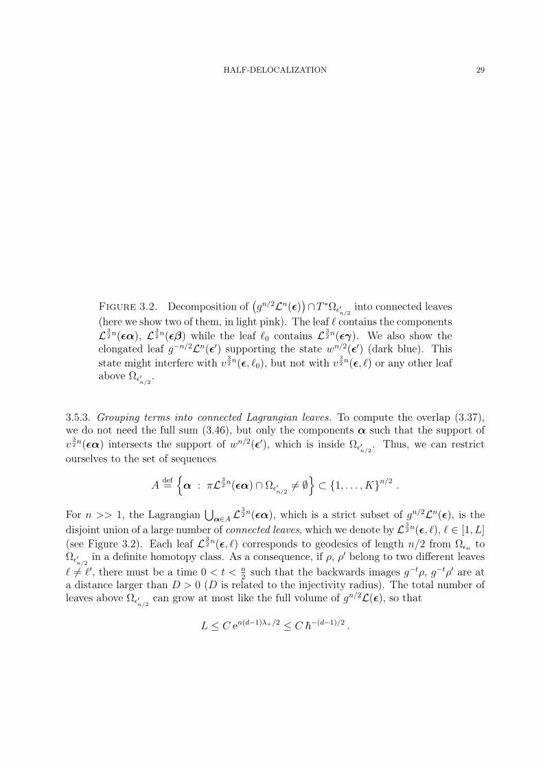
Figure 3.2. Decomposition of(gn/2Ln(ε))∩T ∗Ωε′

n/2into connected leaves

(here we show two of them, in light pink). The leaf ` contains the componentsL 3

2n(εα), L 3

2n(εβ) while the leaf `0 contains L 3

2n(εγ). We also show the

elongated leaf g−n/2Ln(ε′) supporting the state wn/2(ε′) (dark blue). Thisstate might interfere with v

32n(ε, `0), but not with v

32n(ε, `) or any other leaf

above Ωε′n/2

.

3.5.3. Grouping terms into connected Lagrangian leaves. To compute the overlap (3.37),we do not need the full sum (3.46), but only the components α such that the support ofv

32n(εα) intersects the support of wn/2(ε′), which is inside Ωε′

n/2. Thus, we can restrict

ourselves to the set of sequences

Adef=

α : πL 3

2n(εα) ∩ Ωε′

n/26= ∅

⊂ 1, . . . , Kn/2 .

For n >> 1, the Lagrangian⋃

α∈A L32n(εα), which is a strict subset of gn/2Ln(ε), is the

disjoint union of a large number of connected leaves, which we denote by L 32n(ε, `), ` ∈ [1, L]

(see Figure 3.2). Each leaf L 32n(ε, `) corresponds to geodesics of length n/2 from Ωεn to

Ωε′n/2

in a definite homotopy class. As a consequence, if ρ, ρ′ belong to two different leaves` 6= `′, there must be a time 0 < t < n

2such that the backwards images g−tρ, g−tρ′ are at

a distance larger than D > 0 (D is related to the injectivity radius). The total number ofleaves above Ωε′

n/2can grow at most like the full volume of gn/2L(ε), so that

L ≤ C en(d−1)λ+/2 ≤ C ~−(d−1)/2 .


Each leaf L 32n(ε, `) is the union of a certain number of components L 3

2n(εα), and we group

the corresponding sequences α into the subset A` ⊂ 1, . . . , Kn/2:L 3

2n(ε, `) =

⋃α∈A`

L 32n(εα) .

We obviously have A =⊔`A`. All components L 3

2n(εα) with α ∈ A` are generated by the

same phase function S32n(εα)

def= S

32n(ε, `), so that the state

(3.47) v32n(x; ε, `)

def=

∑α∈A`

v32n(x; εα) = b

32n

~ (x; ε, `) ei~S

32 n(x;ε,`)

is a Lagrangian state supported on L 32n(ε, `), with symbol

b32n

~ (x; ε, `) =∑α∈A`

b32n

~ (x; εα) .

By inspection one can check that, at each point ρ ∈ L 32n(ε, `), the above sum over α ∈ A`

has the effect to insert partitions of unity∑

k P2k = 1 at each preimage g−j(ρ), j =

0, . . . , n2− 1. As a result, the principal symbol will satisfy the same type of upper bound

as in (3.22):

|b32n

0 (x; ε, `)| ≤ |bn(g−n/2S (x))| J−12n

S (x)1/2 ≤ C J− 3

2n

S (x)1/2 , with S = S32n(ε, `) .

The same argument holds for the higher-order terms and their derivatives. Besides, becausethe action of g−3n/2 on L 3

2n(ε, `) is contracting, for any x ∈ Ωε′

n/2the Jacobian J−

32n

S (x) isof the order of Ju3

2n(εα), where α can be any sequence in A` (all these Jacobians are of the

same order). Defining

Ju32n(ε, `) = max

α∈A`

Ju32n(εα) ≥ 1

Cminα∈A`

Ju32n(εα) ,

the full symbol b32n

~ (x; ε, `) satisfies similar bounds as in Lemma 3.4:

(3.48) |dmb32n

k (x; ε, `)| ≤ C nm+3k Ju32n(ε, `)1/2 , k ≤ N − 1, m ≤ 2(N − k) .

3.6. Overlaps between the Lagrangian states. Putting together (3.45, 3.47, 3.46),the overlap (3.37) is approximated by the following sum:

⟨U−n/2vn(ε′), Un/2 vn(ε)

⟩=

L∑

`=1

〈wn/2(ε′), v 32n(ε, `)〉+O(~Nδ′/2) , where(3.49)

〈wn/2(ε′), v 32n(ε, `)〉 =

∫e

i~

(S

32 n(x;ε,`)−Sn/2(x;ε′)

)cn/2~ (x; ε′) b

32n

~ (x; ε, `) .(3.50)

Each term is the overlap between the WKB state wn/2(ε′) supported on g−n/2Ln(ε′), andthe WKB state v

32n(ε, `) supported on L 3

2n(ε, `), both Lagrangians sitting above Ωε′

n/2(see


Figure 3.2). The sup-norms of these two states, governed by the principal symbols cn/20 (ε′),b

32n

0 (ε, `), are bounded by

(3.51) ‖wn/2(ε′)‖L∞ ≤ C Jun/2(ε′)1/2, ‖v 3

2n(ε, `)‖L∞ ≤ C Ju3

2n(ε, `)1/2 .

Here C > 0 is independent of all parameters, including the diameter ε of the partition.The integral (3.49) takes place on the support of cn/2~ (x; ε′), that is (see (3.42)), on a setof volume O(Jun/2(ε

′n/2 · · · ε′n)). It follows that each overlap (3.50) is bounded by

(3.52) |〈wn/2(ε′), v 32n(ε, `)〉| ≤ C Jun/2(ε

′)1/2 Ju32n(ε, `)1/2 Jun/2(ε

′n/2 · · · ε′n) .

We show below that the above estimate can be improved for almost all leaves `, when onetakes into account the phases in the integrals (3.50). Actually, for times n ≤ nE(~), there isat most a single term `0 in the sum (3.49) for which the above bound is sharp; for all otherterms `, the phase oscillates fast enough to make the integral negligible. Geometrically,this phase oscillation means that the Lagrangians L 3

2n(ε, `), g−n/2Ln(ε′) ⊂ Ln/2(ε′) are “far

enough” from each other (see Fig. 3.2). The “distance” between two Lagrangians aboveΩε′

n/2is actually measured by the height

H(L 3

2n(ε, `),Ln/2(ε′)) def

= infx∈Ωε′

n/2

|dS 32n(x; ε, `)− dSn/2(x; ε′)| .

The overlap between “distant” leaves can be estimated through a nonstationary phaseargument:

Lemma 3.7. Assume that, for some δ′′ < δ′/2, for some ~ > 0 and some time n ≤ nE(~),the height

H(L 3

2n(ε, `),Ln/2(ε′)) ≥ ~ 1−δ′′

2 .

Then, provided ~ is small enough, the overlap

(3.53) |〈wn/2(ε′), v 32n(ε, `)〉| ≤ C ~Nδ′′

√Jun/2(ε

′)Ju32n(ε, `) .

The constant C > 0 is uniform with respect to ε′, ε and the implicit parameters z, z′, η1, η′1.

Proof. Let us call s(x) = S32n(x; ε, `) − Sn/2(x; ε′) the phase function appearing in the

integral (3.50). Notice that the assumption on the height means that |ds(x)| ≥ ~ 1−δ′′2 for

all x. We then expand the product cn/2~ b32n

~ and keep only the first N terms:

cn/2~ (x; ε′) b

32n

~ (x; ε, `) = a~(x) +RemN(x) , a~(x) =N−1∑

k=0

~k ak(x) .

From the estimates (3.44,3.48), we control the sup-norm of the remainder:

‖RemN‖L∞ ≤ C ~Nδ′/2√Jun/2(ε

′)Ju32n(ε, `) .


Through the Leibniz rule we control the derivatives of ak:

‖ak‖Cm ≤ C nm+3k√Jun/2(ε

′)Ju32n(ε, `) e

n2(m+2k)λ+ , k ≤ N − 1, m ≤ 2(N − k) .

For each k < N and m ≤ 2(N − k), we have at our disposal the following nonstationaryphase estimate [17, Section 7.7]:

∣∣∣∫ak(x) exp

( i~s(x)

)dx

∣∣∣ ≤ C ~m∑

m′≤msupx

( |dm′ak(x)||ds(x)|2m−m′

)

≤ C ~mδ′′−k(1−δ′/2)√Jun/2(ε

′)Ju32n(ε, `) .

Here we used the assumption on |ds(x)| and the fact that δ′′ < δ′/2. By taking m = N −kfor each k and summing the estimate over k, we get:

∣∣∣∫a~(x) exp

( i~s(x)

)dx

∣∣∣ ≤ C ~Nδ′′√Jun/2(ε

′)Ju32n(ε, `) .

Since δ′/2 > δ′′, the remainder RemN yields a smaller contribution, which ends the proof.¤

We now show that there is at most one Lagrangian leaf L 32n(ε, ò) which can be very

close to Ln/2(ε′):Lemma 3.8. Take as above δ′′ < δ′/2, assume the diameter ε is much smaller than theinjectivity radius, and for ~ small enough take n ≤ (1−δ′)| log ~|

λmax.

If there is some ò ∈ 1, . . . , L such that the height H(L 3

2n(ε, ò),Ln/2(ε′)

) ≤ ~ 1−δ′′2 ,

then for any ` 6= ò we must have H(L 3

2n(ε, `),Ln/2(ε′)) > ~ 1−δ′′

2 .

Proof. Assume ab absurdo the existence of ρo ∈ L 32n(ε, ò), ρ ∈ L 3

2n(ε, `) and ρ′1, ρ

′2 ∈

Ln/2(ε′), such that the Riemannian distances d(ρo, ρ′1) ≤ ~1−δ′′

2 and d(ρ, ρ′2) ≤ ~1−δ′′

2 . Whenapplying the backwards flow for times 0 ≤ t ≤ n

2, these points depart at most like

d(g−tρo, d−tρ′1) ≤ C etλ+ ~1−δ′′

2 ≤ C ~δ′/4−δ′′/2 ,

d(g−tρ, d−tρ′2) ≤ C etλ+ ~1−δ′′

2 ≤ C ~δ′/4−δ′′/2 .

Besides, on this time interval the points g−tρ′1, g−tρ′2 remain in the small Lagrangian pieceg−tLn/2(ε′) of diameter ≤ ε, so that d(g−tρo, g−tρ) ≤ ε. Since ε has been chosen small, thiscontradicts the property that the points g−tρo, g−tρ must depart at a distance ≥ D (seethe discussion at the beginning of §3.5.3). ¤

If there exists a leaf ò such that H(L 32n(ε, ò),Ln/2(ε′)) ≤ ~ 1−δ′′

2 , there is a point ρo ∈L 3

2n(ε, ò) such that g−jρo stays at small distance from Ln/2−j(ε′) for all j = 0, . . . , n/2−1,

and therefore satisfies πg−jρo ∈ Ωε′n/2−j

. This shows that the set Aò contains the sequence


(ε′1 · · · ε′n/2)def= ε′. The overlap corresponding to this leaf is bounded as in (3.52), and after

replacing Ju32n(ε, ò) by Ju3

2n(εε′) we obtain

(3.54) |〈wn/2(ε′), v 32n(ε; ò)〉| ≤ C Jun(ε′) Jun(ε)1/2 .

According to the above two Lemmas, all the remaining leaves are “far from” Ln/2(ε′), andtheir contributions to (3.49) sum up to

∑

` 6=ò〈wn/2(ε′), v 3

2n(ε; `)〉 = O(~Nδ′′−(d−1)/2) .

We take N large enough (say, Nδ′′ >> 1), such that this is negligible compared with (3.54).We finally get, whether such an ò exists or not:

|〈U−n/2vn(z′, η′1, ε′), Un/2vn(z, η1, ε)〉| ≤ C Jun(ε′) Jun(ε)1/2 .

To finish the proof of Lemma 3.2, there remains to integrate over the parameters η1, η′1

in (3.35). Since χ(n) (resp. χ(4n)) is supported on an interval of length ~1−δenδ (resp.~1−δe4nδ), the overlap of Lemma 3.2 finally satisfies the following bound:

|〈U−n/2Pε′ δ(4n)j′ (z′), Un/2 Pε δ

(n)j (z)〉| ≤ C ~−(d+1) e5δn ~2−2δ Jun (ε′) Jun (ε)1/2 .

This is the estimate of Lemma 3.2, with c = 2 + 5/λmax. Proposition 3.1 and Theorem 2.7follow. ¤

4. Subadditivity

The aim of this section is to prove Proposition 2.9. It is convenient here to use somenotions of symbolic dynamics. Starting from our partition of unity (Pk)k=1,...,K , we intro-duce a symbolic space Σ = 1, . . . , KN. The shift σ acts on Σ by shifting a sequenceε = ε0ε1 . . . to the left and deleting the first symbol. For ε = (ε0 . . . εn), we denote [ε] ⊂ Σthe subset (n-cylinder) formed of sequences starting with the symbols ε0 . . . εn (throughoutthis section the integer n will generally differ from nE(~)).

To any normalized eigenfunction ψ~ we can associate a probability measure µΣ~ on Σ by

letting, for any n-cylinder [ε],

µΣ~ ([ε])

def= ‖PεnPεn−1(1) . . . Pε0(n)ψ~‖2 = ‖Pεn(−n)Pεn−1(−(n− 1)) . . . Pε0 ψ~‖2 .

If we denote ε = (εnεn−1 · · · ε0), this quantity is equal to ‖P ∗ε ψ~‖2 = ‖P ∗ε ψ~‖2 (see (2.23)).To ensure that this defines a probability measure on Σ, one needs to check the followingcompatibility condition

(4.1) µΣ~ ([ε0 . . . εn]) =

K∑εn+1=1

µΣ~ ([ε0 . . . εnεn+1])

for all n and all ε0 . . . εn. This identity is obvious from (2.4).


4.1. Invariance until the Ehrenfest time. By the Egorov theorem, if µ is the weak-∗limit of the Wigner measures Wψ~ on T ∗M , then for every n and any fixed n-cylinder[ε] ⊂ Σ we have µΣ

~ ([ε])~→0−−→ µ(ε), where ε was defined in §2.2.7 as the function

P 2εn (P 2

εn−1 g1) . . . (P 2

ε0 gn) on T ∗M . This means that the measures µΣ

~ converge to a

measure µΣ0 defined by µΣ

0 ([ε])def= µ(ε).

Since the ψ~ are eigenfunctions, µ is localized on E and is (gt)-invariant (Prop. 1.1), sothat µΣ

0 is σ-invariant. For ~ > 0 the measures µΣ~ are not exactly σ-invariant; yet, we

show below that µΣ~ is almost invariant under the shift, until the Ehrenfest time.

For small γ, ν > 0 we introduce the time Tν,γ,~def= (1−γ)| log ~|

2(1+ν)λmax.

Proposition 4.1. For any given no ∈ N, for any small enough ~ and any n ∈ N such thatn+ no ≤ 2Tν,γ,~, for any cylinder [ε] = [ε0ε1 . . . εno ] of length no, one has

∑εi,−n≤i≤−1

µΣ~ ([ε−n . . . ε−1ε0ε1 . . . εno ]) = µΣ

~ ([ε0ε1 . . . εno ]) +O(~γ/2) .

The implied constant is uniform with respect to no and n in the allowed interval. In otherwords, the measure µΣ

~ is almost σ-invariant:

σn] µΣ~ ([ε])

def= µΣ

~ (σ−n[ε]) = µΣ~ ([ε]) +O(~γ/2) .

Proof. For simplicity we prove the result for no = 0; the argument can easily be adaptedto any no > 0.

We use an estimate on the norm of commutators, proved in Lemma 5.2. If A is anoperator on L2(M), remember that we denote A(t) = U−tAU t. According to Lemma 5.2,for any smooth observables a, b supported inside Eν = E(1/2− ν, 1/2 + ν), one has

(4.2) ‖[Op~(a)(t),Op~(b)(−t)]‖L2(M) = O(~γ) ,

or equivalently

‖[Op~(a)(2t),Op~(b)]‖L2(M) = O(~γ),

for any time |t| ≤ Tν,γ,~. This result will be applied to the observables a = Pε0 f , b = Pεj f ,where f is compactly supported in Eν and identically 1 near E . According to Remark 2.4,inserting the cutoff f after each Pεj only modifies µΣ

~ ([ε]) by an amount O(~∞). In thefollowing, we will omit to indicate these insertions and the O(~∞) errors.


To prove Proposition 4.1, we first write∑

εi,−n≤i≤−1

µΣ~ ([ε−nε−(n−1) . . . ε0]) =

∑εi,−n≤i≤−1

‖Pε0Pε−1(1) . . . Pε−n(n)ψ~‖2

=∑

〈Pε−1(1)P 2ε0Pε−1(1)P ∗[ε−2...ε−n](2)ψ~, P

∗[ε−2...ε−n](2)ψ~〉

=∑

〈P 2ε0Pε−1(1)2P ∗[ε−2...ε−n](2)ψ~, P

∗[ε−2...ε−n](2)ψ~〉

+O(~γ)[ ∑εi,−n≤i≤−2

‖P ∗[ε−2...ε−n](2)ψ~‖2]

=∑

εi,−n≤i≤−2

〈P 2ε0P ∗[ε−2...ε−n](2)ψ~, P

∗[ε−2...ε−n](2)ψ~〉+O(~γ) .

We have used the identities∑

ε−1Pε−1(1)2 = I and

∑ε−n,...,ε−2

‖P ∗[ε−2...ε−n] ψ~‖2 = 1. Werepeat the procedure:

∑εi,−n≤i≤−2

〈P 2ε0P ∗[ε−2...ε−n](2)ψ~, P

∗[ε−2...ε−n](2)ψ~〉

=∑

〈Pε−2(2)P 2ε0Pε−2(2)P ∗[ε−3...ε−n](3)ψ~, P

∗[ε−3...ε−n](3)ψ~〉

=∑

〈P 2ε0Pε−2(2)2P ∗[ε−3...ε−n](3)ψ~, P

∗[ε−3...ε−n](3)ψ~〉

+O(~γ)[ ∑εi,−n≤i≤−3

‖P ∗[ε−3...ε−n](3)ψ~‖2]

=∑

εi,−n≤i≤−3

〈P 2ε0P ∗[ε−3...ε−n](3)ψ~, P

∗[ε−3...ε−n](3)ψ~〉+O(~γ) .

Iterating this procedure n times we obtain∑

εi,−n≤i≤−1

µΣ~ ([ε−nε−(n−1) . . . ε0]) = 〈P 2

ε0ψ~, ψ~〉+ nO(~γ) ,

which proves the Proposition for n0 = 0, since n = O(| log ~|). The proof for any fixedn0 > 0 is identical. ¤

4.2. Proof of Proposition 2.9. For ψ~ an eigenstate of the Laplacian, the entropy hn(ψ~)introduced in (2.12) can be expressed in terms of the measure µΣ

~ :

hn(ψ~) = −∑

|ε|=n‖P ∗ε ψ~‖2 log‖P ∗ε ψ~‖2 = −

∑

|ε|=nµΣ~ ([ε]) log µΣ

~ ([ε])

= −∑

|ε|=nµΣ~ ([ε]) log µΣ

~ ([ε])def= hn(µ

Σ~ ) .

(4.3)

In ergodic theory, the last term is called the entropy of the measure µΣ~ with respect to

the partition of Σ into n-cylinders. Before using the results of the previous section, wechoose the parameters ν, γ appearing in Proposition 4.1 such that ν = γ = δ′/2, where δ′


is the small parameter in Proposition 2.9. This ensures that the time 2Tν,γ,~ ≥ nE(~) (see(2.10)).

We then have, for any no and n such that n+ no ≤ Tν,γ,~,

(4.4) hno+n(µΣ~ ) ≤ hn−1(µ

Σ~ ) + hno(σ

n] µ

Σ~ ) = hn−1(µ

Σ~ ) + hno(µ

Σ~ ) +Ono(~δ

′/4) .

The notation Ono means that the last term is bounded by Cno~δ′/4, with a constant Cno

depending on no. The first inequality is a general property of the entropy, due to theconcavity of the logarithm. The second equality comes from the almost invariance of µΣ

~(Proposition 4.1) and the continuity of the function x 7→ −x log x. The pressure for ψ~(see (2.13)) also involves sums of the type

∑ε=ε0...εno+n

µΣ~ ([ε]) log Juno+n(ε)

def= µΣ

~ (log Juno+n) .

Using the factorization (2.16) of the Jacobian, this sum can be split into

µΣ~ (log Juno+n) = µΣ

~ (log Jun−1) + σn−1] µΣ

~ (log Ju1 ) + σn] µΣ~ (log Juno

)

= µΣ~ (log Jun−1) + µΣ

~ (log Ju1 ) + µΣ~ (log Juno

) +Ono(~δ′/4) .

(4.5)

We used once more the quasi-invariance of µΣ~ to get the second equality. Combining the

inequalities (4.4,4.5) with (4.3), we obtain the Proposition 2.9 with the constant

R = 3 maxρ∈Eε

| log Ju1 (ρ)| .

¤

5. Some results of pseudodifferential calculus

5.1. Pseudodifferential calculus on a manifold. In this section we present the stan-dardWeyl quantization of observables defined on the cotangent of the compact d-dimensionalmanifold M (see for instance [13]). The manifold can be equipped with an atlas f`, V`,such that the V` form an open cover of M , and for each `, f` is a diffeomorphism from V`to a bounded open set W` ⊂ Rd. Each f` induces a pullback f ∗` : C∞(W`) → C∞(V`). Wedenote by f` the induced canonical map between T ∗V` and T ∗W`:

(x, ξ) ∈ T ∗V` 7→ f`(x, ξ) = (f`(x), (Df`(x)−1)T ξ) ∈ T ∗W` ,

(AT is the transposed of A) and by f ∗` : C∞(T ∗W`) → C∞(T ∗V`) the corresponding pull-back. One then chooses a smooth partition of unity on M adapted to the charts V`,namely a set of functions φ` ∈ C∞c (V`) such that

∑` φ` = 1 on M .

Any observable a ∈ C∞(T ∗M) can now be split into a =∑

j a`, with a` = φ` a, eachterm being pushed to a` = (f−1

` )∗a` ∈ C∞(T ∗W`). If a belongs to a nice class of functions(possibly depending on ~), for instance the space of symbols

(5.1) a ∈ Sm,k = Sk(〈ξ〉m)def=

a = a~ ∈ C∞(T ∗M), |∂αx∂βξ a| ≤ Cα,β~−k 〈ξ〉m−|β|

,


then Weyl-quantization associates to each a` a pseudodifferential operator on S(Rd):

(5.2) ∀u ∈ S(Rd) , Opw~ (a`) u(x) =1

(2π~)d

∫e

i~ 〈x−y,ξ〉a`

(x+ y

2, ξ; ~

)u(y) dy dξ .

To pull this pseudodifferential operator back on C∞(V`), one takes a smooth cutoff ψ` ∈C∞c (V`) such that ψ`(x) = 1 close to suppφ`. The quantization of a ∈ Sm,k is finallydefined as follows:

(5.3) ∀u ∈ C∞(M), Op~(a)u =∑

`

ψ` × f ∗` Opw~ (a`) (f−1` )∗(ψ` × u) .

The space of pseudodifferential operators image of Sm,k through this quantization is de-noted by Ψm,k(M). The quantization obviously depends on the cutoffs φ`, ψ`. How-ever, this dependence only appears at second order in ~, and the principal symbol mapσ : Ψm,k(M) → Sm,k/Sm,k−1 is intrinsically defined. All microlocal properties of pseudo-differential operators on Rd are carried over to Ψm,k(M). The Laplacian −~24 belongs toΨ2,0(M), with principal symbol σ(−~24) = |ξ|2x.

We actually need to consider symbols more general than (5.1). Following [10], for any0 ≤ ε < 1/2 we introduce the symbol class

(5.4) Sm,kεdef=

a ∈ C∞(T ∗M), |∂αx∂βξ a| ≤ Cα,β ~−k−ε|α+β| 〈ξ〉m−|β|

.

The induced functions a` will then belong to the corresponding class on T ∗W`, for whichwe can use the results of [10]. For instance, the quantization of any a ∈ S0,0

ε leads to abounded operator on L2(M) (the norm being bounded uniformly in ~).

5.2. Egorov theorem up to logarithmic times. We need analogous estimates to Bouzouina-Robert’s [7] concerning the quantum-classical equivalence for long times. Our setting ismore general, since we are interested in observables on T ∗M for an arbitrary manifold M .On the other hand, we will only be interested in the first order term in the Egorov theorem,whereas [7] described the complete asymptotic expansion in power of ~.

The evolution is given by the propagator U t on L2(M), which quantizes the flow gt onT ∗M . We will consider smooth observables a ∈ C∞c (T ∗M) supported in a thin neighbour-hood of the energy layer E , say inside the energy strip Eν = E([1/2− ν, 1/2 + ν]) for somesmall ν > 0. This strip is invariant through the flow, so the evolved observable at = a gtwill remain supported inside Eν . If λmax is the maximal expansion rate of the flow on E (seethe definition in Theorem 1.2), then by homogeneity the maximal expansion rate inside Eνis√

1 + 2νλmax. If we let λνdef= (1 + ν)λmax, the successive derivatives of the flow on Eν

are controlled as follows:

(5.5) ∀t ∈ R, ∀ρ ∈ Eν , ‖∂αρ gt(ρ)‖ ≤ Cα eλν |α t| .

Obviously, the derivatives of the evolved observable also satisfy

(5.6) ∀t ∈ R, ∀ρ ∈ Eν , ‖∂αat(ρ)‖ ≤ Ca,α eλν |α t| .


For times of the order of | log ~|, each derivative is bounded by some power of ~−1. Moreprecisely, for any γ ∈ (0, 1] and any ~ ∈ (0, 1/2), we call Tν,γ,~ the following time:

(5.7) Tν,γ,~ =(1− γ)| log ~|

2λν=

(1− γ)| log ~|2(1 + ν)λmax

.

Starting from a smooth observable a = a0, the bounds (5.6) show that the family of functionat = a gt : |t| ≤ Tν,γ,~ remains in the symbol class S−∞,0

ε , with ε = 1−γ2. Furthermore,

any quasi-norm is uniformly bounded within the family. To prove a Egorov estimate, westart as usual from the identity

U−t Op~(a)Ut −Op~(a gt) =

∫ t

0

dsU−s (Diff at−s)U s,(5.8)

with Diff atdef=

i

~[−~24,Op~(at)]−Op~(H, at) .(5.9)

Since −~24 belongs to Ψ2,0 ⊂ Ψ2,0ε and Op~(at) ∈ Ψ−∞,0

ε for times |t| ≤ Tν,γ,~, thesemiclassical calculus of [10, Prop. 7.7] (performed locally on each chart Vj) shows thatDiff at ∈ Ψ−∞,−α

ε , with α = 1 − ε = 1+γ2. From the Calderon-Vaillancourt theorem on

Ψ−∞,−αε [10, Thm. 7.11], we extract a constant Ca > 0 such that, for any small enough~ > 0 and any time |t| ≤ Tν,γ,~,

‖Diff at‖ ≤ Ca ~α = Ca ~1+γ2 .

We can finally combine the above estimate in (5.8) and use the unitarity of U t (Duhamel’sprinciple) to obtain the following Egorov estimate.

Proposition 5.1. Fix ν, γ ∈ (0, 1]. Let a be a smooth, ~-independent observable supportedin Eν. Then, there is a constant Ca such that, for any time |t| ≤ Tν,γ,~, one has

(5.10) ‖U−t Op~(a)Ut −Op~(a gt)‖ ≤ Ca |t| ~

1+γ2 .

Let us now consider two observables a, b ∈ C∞c (Eν), evolve one in the future, the other inthe past. The calculus in S−∞,0

ε (with again ε = 1−γ2) shows that, for any time |t| ≤ Tν,γ,~,

one has

[Op~(a gt), Op~(b g−t)] ∈ S−∞,−γε .

Together with the above Egorov estimate and the Calderon-Vaillancourt theorem on Ψ−∞,−γε ,

this shows the following

Lemma 5.2. Fix ν, γ ∈ (0, 1]. Let a, b ∈ C∞c (Eν) be independent of ~. Then there is aconstant C > 0 such that, for small ~ and any time |t| ≤ Tν,γ,~,

‖[U−t Op~(a)Ut, U t Op~(b)U

−t]‖ ≤ C ~γ .


5.3. Cutoff in a thin energy strip. As explained in §2.2.3, we need an energy cutoffχ(0) localizing in the energy strip of width ∼ ~ε around E , with ε ∈ [0, 1) arbitrary close to1. As a result, the m-th derivatives of χ transversally to E will grow like ~−mε. The symbolclasses (5.4) introduced in the previous sections do not include such functions if ε > 1/2.Yet, because the fluctuations occur close to E and only transversally, it is possible to workwith a “second-microlocal” pseudodifferential calculus which includes such fast-varying,anisotropic symbols. We summarize here the treatment of this problem performed in [29,Section 4].

5.3.1. Local behavior of the anisotropic symbols. For any ε ∈ [0, 1), we introduce a class ofsymbols Sm,kE,ε , made of functions a = a~ satisfying the following properties:

• for any family of smooth vectors fields V1, . . . , Vl1 tangent to E , and of smoothvector fields W1, . . . ,Wl2 , one has in each energy strip Eν = E([1/2− ν, 1/2 + ν]):

supρ∈Eν

|V1 . . . Vl1 W1 . . .Wl2 a(ρ)| = O(h−k−ε l2) .

• away from E , we have |∂αx∂βξ a(ρ)| = O(h−k〈ξ〉m−|β|).Notice that Sm,k ⊂ Sm,kE,ε′ ⊂ Sm,kE,ε if 1 > ε > ε′ ≥ 0.

To quantize this class of symbols, we cover a certain neighbourhood Eν of E by a familyof bounded open sets Vj, such that for each j, Vj is mapped by a canonical diffeomorphismκj to a bounded open set Wj ⊂ T ∗Rd, with (0, 0) ∈ Wj. We will denote by (x, ξ) the localcoordinates on Vj ⊂ T ∗M , and (y, η) the image coordinates on Wj. The canonical map κjis chosen such that H κ−1

j = η1 + 1/2. In particular, the image of E ∩ Vj is a piece of thehyperplane η1 = 0.

We consider a smooth cutoff function φ supported inside Eν , with φ ≡ 1 in Eν/2, and asmooth partition of unity (ϕj) such that 1 =

∑j ϕj on ∪jVj, and suppϕj b Vj. For any

symbol a ∈ Sm,kE,ε , the function a(1 − φ) is supported outside Eν/2, and it belongs to thestandard class Sm,k of (5.1). On the other hand, for each index j the function

ajdef= (a φϕj) κ−1

j

is compactly supported inside Wj ⊂ T ∗Rd. That function can be Weyl-quantized as in(5.2). Although aj(y, η) can oscillate at a rate ~−ε along the coordinate η1 near η1 = 0,for a, b ∈ Sm,kE,ε the product Opw~ (aj) Opw~ (bj) is still of the form Opw~ (cj), where the functioncj(y, η) is given by the Moyal product aj]bj and satisfies an asymptotic expansion in powersof ~1−ε and ~.

Mimicking the proof of the Calderon-Vaillancourt theorem in [10, Thm. 7.11], we usethe isometry (in L2(Rd)) between Opw~ (A) and Opw1 (A T~), where the rescalingT~(y, η) = (y1~

1−ε2 , y′~1/2; η1~

1+ε2 , η′~1/2) ensures that the derivatives of aj T~ are uniformly

bounded in ~. As a consequence we get the following

Proposition 5.3. There exist Nd and C > 0 such that the following bound holds. For anysymbol a ∈ Sm,kE,ε and any j, the operator Opw~ (aj) acts continuously on L2(Rd), and its


norm is bounded as follows:

‖Opw~ (aj)‖ ≤ ‖aj‖L∞ + C∑

1≤|α|+|β|≤Nd

~12(|α′|+|β′|+(1−ε)α1+(1+ε)β1) ‖∂αy ∂βη aj‖L∞ .

5.3.2. Global quantization of the anisotropic symbols. We now glue together the variouspieces of a ∈ Sm,kE,ε to define its global quantization. First of all, since a(1 − φ) belongs tothe standard class Sm,k of (5.1), we can quantize it as in §5.1.

Then, for each index j we select a Fourier integral operator Uκj: L2(π(Vj)) → L2(π(Wj)),

elliptic near suppϕj × κj(suppϕj) ⊂ Vj ×Wj, and associated with the diffeomorphism κj(an explicit expression is given in §3.2.1). Since aj describes the symbol a in the coordinates(y, η), it makes sense to pull Opw~ (aj) back to the original coordinates (x, ξ) using Uκj

. Thequantization of the global symbol a ∈ Sm,kE,ε is then defined as follows:

(5.11) OpE,~(a)def= Op~(a(1− φ)) +

∑j

U∗κjOpw~ (aj)Uκj

.

The Fourier integral operators (Uκj) can and will be chosen such that OpE,~(1) = Id +

OL2→L2(~∞). The operators OpE,~(a) make up a space Ψm,kE,ε of pseudodifferential operators

on M . The quantization OpE,~ depends on the choice of the cutoffs φ, ϕj, the diffeomor-phisms κj and the associated FIOs (Uκj

). It is equal to the quantization Op~ for symbolsa supported outside the energy strip Eν ; otherwise, it differs from Op~ by higher-orderterms.

The space Ψ−∞,kE,ε is invariant under conjugation by FIOs which preserve the energy layer

E . We will apply that property to the propagator U = ei~4/2, which quantizes the flow g1.One actually has a Egorov property

U−1 OpE,~(a)U = OpE,~(b) , with b− a g ∈ S−∞,k−1+εE,ε .

One is naturally lead to the definition of an ~-dependent essential support of a symbola~ ∈ Sm,kE,ε (we will only consider the finite part of the essential support, the infinite partat |ξ| = ∞ being irrelevant for our purposes). A family of sets (V~ ⊂ T ∗M)~→0 doesnot intersect ess− suppa~ iff there exists χ~ ∈ S−∞,0

E,ε , with χ~ ≥ 1 on V~, such thatχ~ a~ ∈ S−∞,−∞

E,ε . The essential support of a~ is also the wavefront set of its quantization,WF~(OpE,~(a~)).

The above Egorov property can be iterated to all orders, showing that the wavefront setof an operator A ∈ Ψ−∞,k

E,ε is transported classically:

(5.12) WF~(U−1AU

)= g−1(WF~(A)) .

5.4. Properties of the energy cutoffs. Take some small δ > 0 and Cδ > 0 as in§2.2.3, and define ε = 1 − δ. One can easily check that the cutoffs χ(n) defined in (2.6),with n ≤ Cδ| log ~|, all belong to the symbol class S−∞,0

E,ε . From the above results, theirquantizations Op(χ(n)) = OpE,ε(χ

(n)) are continuous operators on L2(M), of norms

(5.13) ‖Op(χ(n))‖ = 1 +O(~δ/2) ,


with an implied constant independent of n. We want to check that these cutoffs havelittle influence on an eigenstate ψ~ satisfying (2.2). For this, we invoke the ellipticity of(−~24−1) ∈ Ψ2,0 ⊂ Ψ2,0

E,ε away from E . Using [29, Prop. 4.1], one can adapt the standarddivision lemma to show the followingProposition 5.4. For ~ > 0 small enough and any n ∈ N, 0 ≤ n ≤ C| log ~|, there existsA

(n)~ ∈ Ψ−2,ε

E,ε and R(n)~ ∈ Ψ−∞,−∞

E,ε such that

OpE,~(1− χ(n)) = A(n)~ (−~24− 1) +R

(n)~ .

As a result, for any eigenstate ψ~ = −~2 4 ψ~, one has

‖ψ~ −OpE,~(χ(n))ψ~‖ = O(~∞) ‖ψ~‖ .

The implied constant is uniform with respect to n.This result contains in particular the estimate (2.8).

We end this section by proving some properties of the cutoffs χ(n). The general idea isthat an eigenstate ψ~ is localized in an energy strip of width ~, so that inserting cutoffsχ(n) in expressions of the type Op(a)ψ~ has a negligible effect.Lemma 5.5. The following estimates are uniform for ~ > 0 small enough and 0 ≤ n ≤Cδ| log ~|:

‖(1−Op(χ(n+1)))U Op(χ(n))‖ = O(~∞) ,

∀k = 0, . . . , K, ‖(1−Op(χ(n+1)))U Pk Op(χ(n))‖ = O(~∞) .

Here Pk is any element of the partition of unity (2.4).Proof. For the symbols χ(n) the essential support (which has been defined above in a ratherindirect way) coincides with the support. The first statement of the Lemma uses theclassical transport of the wavefront set (5.12), applied to Op(χ(n)). Since χ(n) is invariantthrough the geodesic flow, U Op(χ(n))U−1 has the same wavefront set as Op(χ(n)). Fromthe definition (2.6), the support of (1 − χ(n+1)) is at a distance ≥ C ~ε from the supportof χ(n). The calculus on S0,0

E,ε then implies that the product (1−Op(χ(n+1))) Op(χ(n)) is inΨ−∞,−∞E,ε .The second statement is a consequence of the first: the calculus on Ψ0,0

E,ε, which con-tains the cutoffs Op(χ(n)) and the multiplication operators Pk, shows that Op(χ(n)) andPk Op(χ(n)) have the same wavefront set. ¤

We draw from this Lemma two properties which we use in the text (see (2.5) for thedefinition of Pε).Corollary 5.6. For any sequence ε of length n ≤ Cδ| log ~|, one has

‖(1−Op(χ(n)))Pε Op(χ(0))‖ = O(~∞) .

For any two sequence ε, ε′ of length n ≤ Cδ| log ~|/4, one has

‖(1−Op(χ(4n)))P ∗ε′ Un Pε Op(χn))‖ = O(~∞) .


6. The entropic uncertainty principle: an application of complexinterpolation

In this section we prove the weighted entropic uncertainty principle, namely theorem 2.1,by adapting the original proof of [25].

We consider a complex Hilbert space (H, 〈., .〉), and denote the associated norm by‖ψ‖ =

√〈ψ, ψ〉. The same notation ‖·‖ will also be used for the operator norm on L(H).

Let (αk)k=1,...,N be a family of positive numbers. We consider the weighted lp–norms onHN 3 Ψ = (Ψ1, . . . ,ΨN ):

(6.1) ‖Ψ‖(α)p

def=

( N∑

k=1

αp−2j ‖Ψk‖p

)1/p

, 1 ≤ p <∞ , and ‖Ψ‖(α)∞

def= max

k(αk ‖Ψk‖) .

For p = 2, this norm does not depend on (αk) and coincides with the Hilbert norm derivingfrom the scalar product

〈Ψ,Φ〉HN =∑

k

〈Ψk,Φk〉H.

If Ψ ∈ HN has Hilbert norm unity, we define its entropy as

h(Ψ) = −N∑

k=1

‖Ψk‖2 log‖Ψk‖2 ,

and its pressure with respect to the weights (αk) is defined by

(6.2) pα(Ψ) = −N∑

k=1

‖Ψk‖2 log‖Ψk‖2 −N∑

k=1

‖Ψk‖2 logα2k .

This is the derivative of ‖Ψ‖(α)p with respect to p, evaluated at p = 2.

Similarly, let (βj)j=1,...,M be a family of weights. They induce the following l(β)p –norms

on HM 3 Φ = (Φ1, . . . ,ΦM):

(6.3) ‖Φ‖(β)p

def=

( M∑j=1

βp−2j ‖Φj‖p

)1/p

, 1 ≤ p <∞ , and ‖Φ‖(β)∞

def= max

j(βj ‖Φj‖) .

We can define the entropy of a normalized vector Φ ∈ HM, and its pressure pβ(Φ) withrespect to the weights (βj)j=1,...,M. The standard lp − lq duality [12, Thm.IV.8.1] reads asfollows in the present context:

Proposition 6.1. For any 1 < p, q <∞ such that 1p

+ 1q

= 1, then

(6.4) sup‖Ψ‖(α)

p =1

|〈Λ,Ψ〉| = ‖Λ‖(α)q .


6.1. Complex interpolation. A bounded operator T : HN → HM can be representedby a M×N matrix (Tj k) of bounded operators on H. For 1 ≤ p, q ≤ ∞ we denote by‖T‖(α,β)

p,q the norm of T from l(α)p (HN ) to l(β)

q (HM). We assume that ‖T‖2,2 = 1, whichimplies in particular that ‖Tjk‖ ≤ 1 for all k, j.

Example 1. Suppose we have two partitions of unity (πk)Nk=1 and (τj)

Mj=1 on H, that is,

two families of operators such that

(6.5)N∑

k=1

πkπ∗k = Id,

M∑j=1

τjτ∗j = Id.

The main example we have in mind is the case where U is a unitary operator on H andTj k

def= τ ∗j Uπk.

Let O be a bounded operator on H, and let ϑ ≥ 0. We will be interested in the actionof T on the cone

C(O, ϑ) = Ψ ∈ HN , ‖OΨk −Ψk‖ ≤ ϑ‖Ψ‖2 for all k = 1, . . . ,N ⊂ HN .

Notice that the cone C(O, ϑ) coincides with HN in the special case O = Id, ϑ = 0, whichis already an interesting case.

We introduce the positive number

cO(T ) = maxj,k

αkβj‖TjkO‖L(H) ,

and also A = maxk αk, B = maxj βj. The following theorem extends the result of [25].

Theorem 6.2. For all Ψ ∈ C(O, ϑ) such that ‖Ψ‖2 = 1 and ‖TΨ‖2 = 1, we have

pβ(TΨ) + pα(Ψ) ≥ −2 log(cO(T ) +NABϑ)

.

The proof of this theorem follows the standard proof of the Riesz-Thorin theorem [12,sec.VI.10]. In particular, one uses the following convexity property of complex analyticfunctions.

Lemma 6.3 (3-circle theorem). Let f(z) be analytic and bounded in the strip 0 < x < 1,and continuous on the closed strip. Then, the function logM(x) = log supy∈R |f(x+ iy)|is convex in the interval 0 ≤ x ≤ 1.

We will define an appropriate analytic function in the unit strip. Let Ψ ∈ C(O, ϑ) with‖Ψ‖2 = 1. Fix t ∈ [0, 1], close to 0, and let

Ψ =Ψ

‖Ψ‖(α)2

1+t

.

From the definition of the norm and Hölder’s inequality, we have

‖Ψ‖(α)2

1+t

≥ A−t .


Consider any state Φ ∈ HM such that ‖Φ‖(β)2

1+t

≤ 1. For each z = x + iy in the strip0 ≤ x ≤ 1, we define

a(z) =1 + z

1 + t,

and the states

Ψ(z) =(Ψ(z)k = Ψk‖Ψk‖a(z)−1α

a(z)−1k

)k=1...N

,

Φ(z) =(Φ(z)j = Φj‖Φj‖a(z)−1β

a(z)−1j

)j=1...M

.

By construction, we have

∀z = x+ iy, ‖Ψ(z)‖(α)2

1+x

= 1 and ‖Φ(z)‖(β)2

1+x

≤ 1 .

In particular, for any y ∈ R we have

(6.6) ‖Ψ(iy)‖2 = 1 and ‖Φ(iy)‖2 ≤ 1 =⇒∣∣∣〈T Ψ(iy),Φ(iy)〉

∣∣∣ ≤ ‖T‖2,2 .

Similarly, for any y ∈ R,‖Φ(1 + iy)‖(β)

1 ≤ 1 =⇒∣∣〈T Ψ(1 + iy),Φ(1 + iy)〉

∣∣ ≤ ‖T Ψ(1 + iy)‖(β)∞ .

We decompose the right hand side by inserting the operator O:

‖T Ψ(1 + iy)‖(β)∞ = max

jβj‖

∑

k

TjkΨ(1 + iy)k‖

≤ maxjβj‖

∑

k

TjkOΨ(1 + iy)k‖+ maxjβj‖

∑

k

Tjk(Id−O)Ψ(1 + iy)k‖ .

The first term on the right hand side is bounded above by cO(T )‖Ψ(1 + iy)‖(α)1 = cO(T ).

For the second term, we remark that

‖Ψ(1 + iy)k‖ = |αk|1−t1+t‖Ψk‖

21+t =

|αk|1−t1+t‖Ψk‖

21+t

(‖Ψ‖(α)2

1+t

) 21+t

.

On the one hand, ‖Ψk‖ ≤ ‖Ψ‖2 ≤ 1 and |αk|1−t1+t ≤ A

1−t1+t . On the other hand we have

already stated that ‖Ψ‖(α)2

1+t

≥ A−t. Putting these bounds together and using the fact thatΨ ∈ C(O, ϑ), we get

∀k = 1, . . . ,N , ‖(Id−O)Ψ(1 + iy)k‖ ≤ Aϑ .

Summing over k and using ‖Tjk‖ ≤ 1, we find

maxjβj‖

N∑

k=1

Tjk(Id−O)Ψ(1 + iy)k‖ ≤ N AB ϑ .

We have proved that for all y ∈ R,(6.7)

∣∣〈T Ψ(1 + iy),Φ(1 + iy)〉∣∣ ≤ cO(T ) +N AB ϑ .


The function z 7→ 〈T Ψ(z),Φ(z)〉 is bounded and analytic in the strip 0 ≤ x ≤ 1: this isthe function to which we apply the 3-circle theorem (Lemma 6.3). Taking in to account(6.6,6.7), we obtain for any x ∈ [0, 1], y ∈ R,

log∣∣〈T Ψ(x+ iy),Φ(x+ iy)〉

∣∣ ≤ (1− x) log‖T‖2,2 + x log(cO(T ) +NABϑ)

≤ x log(cO(T ) +NABϑ)

.

The last inequality is due to our assumption ‖T‖2,2 = 1. In particular, taking x + iy = t,and exponentiating, we get

∣∣〈T Ψ,Φ〉∣∣ ≤ (cO(T ) +NABϑ)t

.

Taking the supremum over

Φ ∈ HM, ‖Φ‖(β)2

1+t

≤ 1

and using the l(β)

21+t

− l(β)

21−t

duality(Prop. 6.1), we obtain

‖T Ψ‖(β)2

1−t

≤ (cO(T ) +NABϑ)t

,

and by homogeneity

(6.8) ‖TΨ‖(β)2

1−t

≤ (cO(T ) +NABϑ)t ‖Ψ‖(α)

21+t

.

We may now take the limit t → 0 in this inequality. Using the assumption ‖Ψ‖2 = 1, wenotice that

log‖Ψ‖(α)2

1+t

∼ 1 + t

2log

(∑

k

‖Ψk‖2 exp−t log‖Ψk‖2 − t logα2k

)∼ t

2pα(Ψ).

Similarly, log‖TΨ‖(β)2

1−t

∼ − t2pβ(TΨ). Therefore, in the limit t → 0, (6.8) implies Theo-

rem 6.2.¤

6.2. Specialization to particular operators T and states Ψ. We now come back tothe case of Example 1.

Lemma 6.4. Let U : H → H be a bounded operator. Using the two partitions of Example 1,we construct the operator T : HN → HM through its components Tjk = τ ∗j Uπk. Then thetwo following norms are equal:

‖T‖2,2 = ‖U‖L(H) .

Proof. The operator T may be described as follows. Consider a line and column vectors ofoperators on H:

Ldef= (π1, . . . , πN) , respectively C =

τ ∗1...τ ∗M

.

We can write T = CUL. We insert this formula in the identity

‖T‖22,2 = ‖T ∗T‖L(HN ) = ‖L∗U∗C∗CUL‖L(HN )


Using the resolution of identity of the τj, we notice that C∗C = IdH, so that the abovenorm reads

‖L∗U∗UL‖L(HN ) .

Then, using the resolution of identity of the πk, we get

‖(UL)∗(UL)‖L(HN ) = ‖(UL)(UL)∗‖L(H) = ‖(UL)L∗U∗‖L(H) = ‖UU∗‖L(H) .

¤Therefore, if U is contracting (resp. ‖U‖L(H) = 1) one has ‖T‖2,2 ≤ 1 (resp. ‖T‖2,2 = 1).We also specialize the vector Ψ ∈ HN by taking Ψk = π∗kψ for some normalized ψ ∈ H.

From the resolution of identity on the πk, we check that ‖Ψ‖2 = ‖ψ‖, and also (TΨ)j =τ ∗j Uψ. Thus, if ‖Uψ‖ = 1, the second resolution of identity induces ‖TΨ‖2 = ‖Uψ‖ = 1.With this choice for T and Ψ, Theorem 6.2 reads as follows:

Theorem 6.5. We consider the setting of Example 1. Let U be an isometry on H.Define c(α,β)

O (U)def= supj,k αkβj‖τ ∗j U πk O‖L(H).

Then, for any normalized ψ ∈ H satisfying

∀k = 1, . . . ,N , ‖(Id−O)π∗kψ‖ ≤ ϑ ,

and defining the pressures as in (6.2), we have

pβ((τ ∗j Uψ)j=1...M

)+ pα

((π∗kψ)k=1...N

) ≥ −2 log(c(α,β)O (U) +N AB ϑ

).

This theorem implies Theorem 2.1, if we take the same partition π = τ (in particularN = M), and if we remark that the pressures pα

((π∗kψ)k=1...N

)and pβ

((π∗jUψ)j=1...N

)are

the same as the quantities pπ,α(ψ), pπ,β(Uψ) appearing in the theorem.

References

[1] N. Anantharaman, Entropy and the localization of eigenfunctions, to appear in Ann. of Math.(2007)

[2] N. Anantharaman, S. Nonnenmacher, Entropy of semiclassical measures of the Walsh-quantizedbaker’s map, Ann. H. Poincaré 8, 37–74 (2007)

[3] N. Anantharaman, H. Koch and S. Nonnenmacher, Entropy of eigenfunctions, to appear in theProceedings of the International Congress on Mathematical Physics - Rio de Janeiro, August 6 -11, 2006.

[4] P. Bérard, On the wave equation on a compact Riemannian manifold without conjugate points,Math. Z. 155, 249–276 (1977).

[5] M.V. Berry, Regular and irregular semiclassical wave functions, J.Phys. A 10, 2083–2091 (1977)[6] O. Bohigas, Random matrix theory and chaotic dynamics, in M.J. Giannoni, A. Voros and J. Zinn-

Justin eds., Chaos et physique quantique, (École d’été des Houches, Session LII, 1989), NorthHolland, 1991

[7] A. Bouzouina and D. Robert: Uniform Semi-classical Estimates for the Propagation of QuantumObservables, Duke Math. J. 111, 223–252 (2002)

[8] Y. Colin de Verdière, Ergodicité et fonctions propres du laplacien, Commun. Math. Phys. 102,497–502 (1985)

[9] Y. Colin de Verdière, B. Parisse, Équilibre instable en régime semi-classique I : concentrationmicrolocale, Commun. Partial Differential Equations 19 no. 9-10, 1535–1563 (1994)


[10] M. Dimassi, J. Sjöstrand, Spectral asymptotics in the semi-classical limit, London MathematicalSociety Lecture Note Series, 268. Cambridge University Press, Cambridge, 1999.

[11] H. Donnelly, Quantum unique ergodicity, Proc. AMS 131, 2945–2951 (2002)[12] N. Dunford and J.T. Schwartz, Linear Operators, Part I, Interscience, New York, 1958.[13] L.C. Evans and M. Zworski, Lectures on semiclassical analysis (version 0.2), available at

http://math.berkeley.edu/∼zworski[14] F. Faure, S. Nonnenmacher and S. De Bièvre, Scarred eigenstates for quantum cat maps of

minimal periods, Commun. Math. Phys. 239, 449–492 (2003).[15] F. Faure and S. Nonnenmacher, On the maximal scarring for quantum cat map eigenstates,

Commun. Math. Phys. 245, 201–214 (2004).[16] J. Hadamard, Le problème de Cauchy et les équations aux dérivées partielles linéaires hyper-

boliques, Paris, Hermann 1932.[17] L. Hörmander, The analysis of linear partial differential operators I, Springer (Heidelberg), 1983.[18] A. Katok and B. Hasselblatt, Introduction to the modern theory of dynamical systems, Encyclo-

pedia of Mathematics and its applications vol.54, Cambridge University Press, 1995.[19] D. Kelmer, Arithmetic quantum unique ergodicity for symplectic linear maps of the multidimen-

sional torus, to appear in Ann. of Math., math-ph/0510079[20] D. Kelmer, Scarring on invariant manifolds for perturbed quantized hyperbolic toral automor-

phisms, preprint, arXiv:math-ph/0607033[21] W.P.A. Klingenberg, Riemannian manifolds with geodesic flows of Anosov type, Ann. of Math.

(2) 99, 1–13 (1974)[22] K. Kraus, Complementary observables and uncertainty relations, Phys. Rev. D 35, 3070–3075

(1987)[23] F. Ledrappier, L.-S. Young, The metric entropy of diffeomorphisms. I. Characterization of mea-

sures satisfying Pesin’s entropy formula, Ann. of Math. (2) 122 (1985), no. 3, 509–539.[24] E. Lindenstrauss, Invariant measures and arithmetic quantum unique ergodicity, Annals of Math.

163, 165-219 (2006)[25] H. Maassen and J.B.M. Uffink, Generalized entropic uncertainty relations, Phys. Rev. Lett. 60,

1103–1106 (1988)[26] S. Nonnenmacher and M. Zworski, Quantum decay rates in chaotic scattering, preprint 2007,

arXiv:0706.3242[27] Z. Rudnick and P. Sarnak, The behaviour of eigenstates of arithmetic hyperbolic manifolds, Com-

mun. Math. Phys. 161, 195–213 (1994)[28] A. Schnirelman, Ergodic properties of eigenfunctions, Usp. Math. Nauk. 29, 181–182 (1974)[29] J. Sjöstrand and M. Zworski, Asymptotic distribution of resonances for convex obstacles, Acta

Math. 183, 191–253 (1999)[30] A. Voros, Semiclassical ergodicity of quantum eigenstates in the Wigner representation, Lect.

Notes Phys. 93, 326-333 (1979) in: Stochastic Behavior in Classical and Quantum HamiltonianSystems, G. Casati, J. Ford, eds., Proceedings of the Volta Memorial Conference, Como, Italy,1977, Springer, Berlin

[31] S.A. Wolpert, The modulus of continuity for Γ0(m)/H semi-classical limits, Commun. Math.Phys. 216, 313–323 (2001)

[32] S. Zelditch, Uniform distribution of the eigenfunctions on compact hyperbolic surfaces, DukeMath. J. 55, 919–941 (1987)

Unité de Mathématiques Pures et Appliquées, École Normale Supérieure, 6, alléed’Italie, 69364 LYON Cedex 07, France

E-mail address: [email protected]


Service de Physique Théorique, CEA/DSM/PhT, Unité de recherche associé CNRS,CEA/Saclay, 91191 Gif-sur-Yvette, France

E-mail address: [email protected]

half-delocalization of eigenfunctions for the …irma.math.unistra.fr/~anantharaman/lap12.pdf ·...

Documents