volatility forecast combination of brazilian selic ... · volatility forecast combination of...

Volatility Forecast Combination of Brazilian Selic interest rate and exchange rate by means of Principal Component Analysis

LIZANDRA SALAU DA ROCHA* ADRIANO MENDONÇA SOUZA*

ROSELAINE RUVIARO ZANINNI* MEIRE MEZZOMO **

*Department of Statistics, Federal University of Santa Maria, Av. Roraima, 1000, Santa Maria, Brazil.

[email protected], [email protected], [email protected] **Department of Informatics and statistics, Federal University of Santa Catarina, Av. Campus

University Rector John David Ferreira Lima Trindade, Florianópolis, Brazil. [email protected]

Abstract: - Using volatility models for macroeconomic variables can provide more efficient results than models which estimate the average of the process. In this context, the purpose of this research was to evaluate the efficiency of individual models and combination models in forecasting the Brazilian SELIC interest rate and exchange rate between January, 1974 and June, 2012 and from January, 1980 to May, 2012, respectively. The analysis of the series confirmed the presence of volatility in those periods, where Brazil’s economic scenario, marked by both internal and external crises, was decisive for such variance. For this purpose, joint modeling was used for the average (ARIMA) and variance (ARCH, GARCH, EGARCH, TARCH) of the process. The results showed that, in general, the performance measures considered (MAPE, MSE, and U-THEIL) are better for forecast combinations. In addition, forecast combinations by PCA using different kinds of weighting were not conclusive for the kinds of weighting used. This shows that when forecast combination by the PCA method is performed, the best alternative is to use more than one type of PCA in order to obtain the best results.

Key-Words: - time series, volatility models, selic interest rate, exchange rate, forecast combination, pca method. 1 Introduction In a country’s economic scenario, the behavior of macroeconomic variables, such as interest rate and exchange rate, can influence other variables and change the economy’s performance. The interest rate, for example, plays a significant role in the economy by influencing economic agents, and exchange rate fluctuations directly influence country’s imports and exports, thus affecting the balance of trade. The assessment and measurement of variance within macroeconomic variables is not a simple task, because these variables are closely associated with other variables that depend not only on the Brazilian scenario, but also on the international scenario. However, many studies are currently being conducted to find models where estimates can reflect reality more accurately. These models started

being developed in the 1980 to measure, analyze and forecast the volatility intrinsic to the financial and/or macroeconomic series to reduce the risks of previous investment while trying to increase the expected return, as opposed to previous econometric models that focused on the first condition only. Thus, measuring the variance of economic series allows decision-makers to obtain better results, reducing risks inherent in financial transactions. Although volatility models are widely applicable to economic series, their use is not restricted; several economic variables use this kind of modeling because they have volatile properties in the series. The use of models that capture the volatility of the series are important because there are time series whose behavior typically features volatility clustering, i.e., periods in which the variable shows great fluctuations for a long period of time followed

WSEAS TRANSACTIONS on BUSINESS and ECONOMICSLizandra Salau Da Rocha, Adriano Mendonça Souza,

Roselaine Ruviaro Zaninni, Meire Mezzomo

E-ISSN: 2224-2899 514 Volume 11, 2014

mailto:[email protected]



by moments of relative calm. This justifies the use of such models, which enables research on the process that generates the series, producing consistent results because of the stability of the series over time. The macroeconomic series used in this research are the SELIC interest rate and the exchange rate. These series were chosen because they have a strong influence on economic activity and change companies willingness to invest. The economic literature provides many volatility forecasting models with the aim of forecasting variance more accurately. The most prominent volatility models are known as the ARCH family models. According to Engle [7], Bollerslev [1], Nelson [15], Zakoian [26] and Bueno [2], volatility models have been developed over time, creating terms and parameters that did not exist in their predecessors. Thus, volatility modeling gradually improved and acquired properties of volatile series that had not been captured by early models. In this way, each volatility model has preserved its own properties and contains the parameters that can determine conditional variance (volatility). According to Rausser and Oliveira [19], Libby and Blashfield [14], Makridakis and Winkler [16] and Werner [25], it is known that forecast combination produces better results than individual models when the level of a time series is forecasted. Thus, the research hypothesis of this study is to verify whether or not forecast combination is also better when applied to volatility models. It also investigates whether or not the use of principal component analysis (PCA) as a way of weighting the different models produces efficient results in the composition of the weights of the combination, as well as in dimensionality reduction. The objective of this study was to make the forecast combination of the exchange rate and the SELIC interest rate by using the models ARCH, GARCH, EGARCH, and TARCH, using the weights obtained by principal component analysis as the weighting factor, and verifying which method is the best to perform forecast combination, compared with others methods of combination. This paper is organized as follows: Section 2 describes volatility models; Section 3 presents performance criteria; Section 4 on describes the methods for forecast combination used in this study; Section 5 contains the analysis and discussion; and Section 6 makes the final considerations, which are followed by the references. 2 Volatility Models

Many mathematical models are used for researching the volatility of financial series, and such models assume that conditional heteroscedasticity exists, that is, non constant variance in the residuals from linear models or from non autocorrelated series. 2.1 ARCH Model In the literature, models are commonly used to capture intrinsic volatility in financial time series because they allow capturing the behavior of variance in the series, which reveals the risk of making decisions towards these variables as well as the return of such variables, usually the price of assets, interest rates, exchange rates, among others. The - ARCH (p) – model, proposed by Engle in 1982 [7], seeks to estimate volatility by using the variance of previous errors. According to Souza, Souza, and Menezes [23], this kind of model emerges because the series depends on the residuals of the estimation of the process average. Thus, variance is observed to emerge from the volatility that exists between the periods of the residuals.

Where errors are independent and identically distributed with mean 0 and variance 1.

Where p corresponds to the model order; is the autoregressive component of the quadratic residuals of the model (ARCH parameter); correspond to non-serially autocorrelated residuals. This model must satisfy the assumption that the conditional variance must be positive; thus, the parameter must satisfy the following assumptions:

> 0 and > 0 and so that the assumption of stationarity is satisfied [3]. 2.2 GARCH Model Bollerslev [1] has proposed the Generalized Autoregressive Conditional Heteroscedasticity (GARCH) model, where the author included the past variance of the series into the ARCH model. This way, the model captures the effects of the quadratic errors and of the variance itself at the past instants. Thus, it is possible to obtain a more



E-ISSN: 2224-2899 515 Volume 11, 2014

economic model, free from the estimation problems of the ARCH model, as shown in equation 4:

Which can be rewritten as:

Where ,and ensuring that . Being able to be rewritten as:

2.3 EGARCH Model Nelson [15] has proposed an extension of the GARCH model, the Exponential GARCH (EGARCH), which captures the asymmetric effects of random shocks suffered by the series. These shocks tend to influence the variance of the series, and there is a difference of impact of these shocks compared to their impact signal. However, negative shocks are usually known to cause greater impact on volatility [24]. For this reason, this model can verify if positive or negative shocks influence volatility with the same weight.

Where Nelson [15] uses the logarithm (ln) of variance described in equation 6, thus modifying, the formulation of the model, besides including the term that captures the asymmetry of the series.

Where εt i.i.d. (0.1).

The parameter γ adjusts the asymmetry of the effects, evidencing that negative and positive shocks produce a different impact on the volatility of the series. If the effect of leverage is observed, with negative shocks (bad news) causing a greater impact on volatility than positive ones (good news), the parameter must be: . 2.4 TARCH Model The asymmetries in volatility can be captured by the model developed by [26]. This model is another variant of the GARCH model, referred to as TARCH by some researchers. In the financial markets, there are periods of price downfalls which are often followed by periods of intense volatility, while in periods of price increases, volatility is not so intense. This effect is designated as leverage. The conditional variance of the TARCH (Threshold Autoregressive Conditional Heteroscedasticity) model (p, q) can be defined by:

Where

If = 0, there is no asymmetry in the conditional variance. Negative market forecasts ( ), such as an abrupt dollar downfall or political instability, have an impact of while positive information ( ), for example, intense demand for an asset, has an impact α. To confirm the leverage effect for this model, The use of these models favors the behavior analysis of the time series, jointly estimating the average and the process variance, enabling distinct models to capture different behaviors, since the models are not excluding; they are able to complement each other. 3 Evaluation Criteria This section describes the methodological steps as a way to test the research hypothesis, which is the use of principal component analysis (PCA) as a way to weight the forecast combination, and achieve the



E-ISSN: 2224-2899 516 Volume 11, 2014

research objective, which is to perform the forecast combination for the volatility of the series of interest rate and SELIC rate, in order to obtain the better results than the models previously used. First, the series was estimated by the linear models of the ARIMA general class; later, a series of residuals is obtained, with such series presenting the characteristics of white noise. Volatility is then estimated by the models of the ARCH family. This way, the ARIMA-ARCH mixed model is obtained. After estimating various models for the series, the Akaike Information Criterion (AIC) and the Bayesian Information Criterion (BIC) penalization criteria are used to help to choose the best model, using the maximized value of the Likelihood Function for the estimated model (L), the number of parameters (n) and the size of the sample (T) [23].

As described by Diebold and Lopez [6], there are other evaluation criteria that help to evaluate the performance of the forecasting models. These indicators evaluate precision capacity. Among the accuracy evaluation measures available in the literature, the expressions 12, 13, and 14 will be used; they respectively correspond to: mean absolute percentage error (MAPE), mean squared error (MSE) and U-Theil statistics.

Where n corresponds to the number of standard forecasts carried out, represents the real value at instant i, and represents the value forecast at instant i. 4 Forecast Combination Techniques

To carry out the forecast combination of the interest rate and exchange rate, the ARCH, GARCH, EGARCH and TARCH individual models were used to obtain the best estimates and consequently the best values forecasted by each model, following the MAPE, MSE, and U-Theil criteria. To compose the proposed combinations, principal component analysis (PCA), Simple Average (SA) and the Ordinary Least Squares (OLS) method will be used. The first forecast combination technique is PCA, first proposed by Pearson [18] and later by Hotelling [13]. Other researchers, such as Morrison [17], Seber [22], Reinsel [20], and Jackson [11];[12], showed that this method enables the reduction of the data set to be analyzed, for example, when the data are composed by a great number of interrelated variables. When the set of original variables are transformed into a new set that keeps, at most, the variance of the data set, reduction of information takes place. This new set of transformed variables is called Principal Components (PC), which are independent and non-correlated, thus favoring analysis, especially when many variables have to be analyzed [21]. Each principal component is represented by equation 15:

Where the vector of constants that must keep the normality condition. Forecast combination by the PCA method will be carried out by choosing the best individual models out of the four different models - ARCH, GARCH, EGARCH, TARCH. PCA will be performed with the forecasts within the samples of each model previously mentioned. This analysis will allow the construction of weights for each model in the principal components in addition to the weighting of eigenvalues. The principal component analysis allows the use of more than one weighting factor, which can provide the weights given by the factor loading or factor loadings based on the correlation of the variables - which in this study are models of the ARCH family, or the Variable Contributions weight or contribution of the variables also based on the correlations of the models in each PC. Besides these considerations, weighting will also be used to explain each component as performed by Casarin et al [4]. In addition, verification can take place through the correlation matrix between the PCs and the estimates of the models to find out which model has



E-ISSN: 2224-2899 517 Volume 11, 2014

greater representation in each component, thus forming the combination based on the strength of expression of each model. The formulation of the CPs principal components is described in equation 16. (16) Where is the the factor loadings or the contribution of the models, and is the variables that form the linear combination. Besides, it should be noted that the components to be used in the present research will be the significant ones, that is, the ones whose eigenvalues are bigger than one

. The forecast combination by PCA will be given by three different weightings to verify if any of the weightings provides a better forecast result according to the performance indicators. The weights of the first combination by PCA will consider the values given by the matrix of factor loadings shown in equation 17. The second PCA is given by weighting the contribution of models in the components represented by equation 18. The third and final PCA combination will be given considering the weight of the explanation of each component according to equation 19.

Considering that X1, X2, ..., Xn are the variables, represented by the ARCH family models; correspond to the factorial load or the correlation between the PCs and the forecasts of the models used; aij correspond to the contribution of each one of the models in the formation of the PC, that is, the weight that each model has on the formation of the PC, and represents the eigenvalues referring to the main component and that represents the variance corresponding to the explanation of each component. In this study, eigenvalues bigger than one were selected. The second combination technique to be used was proposed by Gupta and Wilton in [9], and it is based

on the arithmetic mean of the forecast models as shown below by expression 20.

Where is the forecast combination, correspond to the forecasts of the individual models and n is the number of individual models used in the combination. According to Makridakis and Winkler [16], using a combination of arithmetic average is better than using the forecast of a bad model. This method is one of the most frequently used in the literature for the sake of convenience and because of the good results it generates compared to individual analyses. The third technique is the estimation by Ordinary Least Squares (OLS) method, having as regressors the forecasts of individual models and as a dependent variable, the differenced series that gave rise to each model, where it is known that each regressor will have a weight factor to be estimated by considering the time horizon used in the forecast.

Where corresponds to the linear coefficient of the regression; is the angular coefficient, the one which will give the weight to each model (regressor); Using the forecast combination by the techniques mentioned above aims to produce better results than those achieved by using individual models. In addition, it can also show which combination method provides better forecast performance, considering the series under study. Soon after volatility was modeled with ARCH models, the principal component analysis will be used for the combination of forecasts formulating three different kinds of combination by PCA, considering the weight factors: factor loading, the contribution of models and eigenvalues. These will be evaluated jointly to verify which kind of weighting works best. Furthermore, the combinations by PCA will be compared to combinations by OLS and Arithmetic Mean, and also the individual models. These comparisons will be made by the following performance criteria: MAPE, MSE and U-THEIL. The combined forecasts are expected to have better results than individual forecasts. In addition, it is believed that the combination by PCA will provide better results than the others for all criteria because of the differenced method to obtain the weights.



E-ISSN: 2224-2899 518 Volume 11, 2014

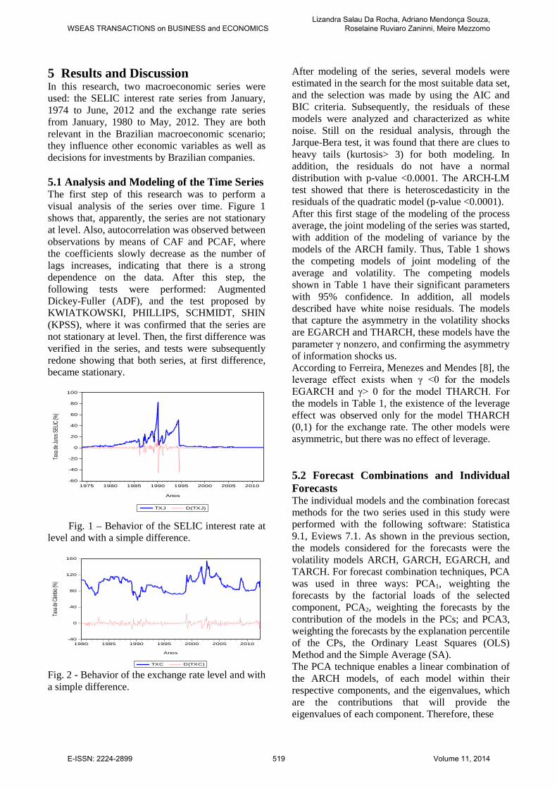
5 Results and Discussion In this research, two macroeconomic series were used: the SELIC interest rate series from January, 1974 to June, 2012 and the exchange rate series from January, 1980 to May, 2012. They are both relevant in the Brazilian macroeconomic scenario; they influence other economic variables as well as decisions for investments by Brazilian companies. 5.1 Analysis and Modeling of the Time Series The first step of this research was to perform a visual analysis of the series over time. Figure 1 shows that, apparently, the series are not stationary at level. Also, autocorrelation was observed between observations by means of CAF and PCAF, where the coefficients slowly decrease as the number of lags increases, indicating that there is a strong dependence on the data. After this step, the following tests were performed: Augmented Dickey-Fuller (ADF), and the test proposed by KWIATKOWSKI, PHILLIPS, SCHMIDT, SHIN (KPSS), where it was confirmed that the series are not stationary at level. Then, the first difference was verified in the series, and tests were subsequently redone showing that both series, at first difference, became stationary.

Fig. 1 – Behavior of the SELIC interest rate at level and with a simple difference.

Fig. 2 - Behavior of the exchange rate level and with a simple difference.

After modeling of the series, several models were estimated in the search for the most suitable data set, and the selection was made by using the AIC and BIC criteria. Subsequently, the residuals of these models were analyzed and characterized as white noise. Still on the residual analysis, through the Jarque-Bera test, it was found that there are clues to heavy tails (kurtosis> 3) for both modeling. In addition, the residuals do not have a normal distribution with p-value <0.0001. The ARCH-LM test showed that there is heteroscedasticity in the residuals of the quadratic model (p-value <0.0001). After this first stage of the modeling of the process average, the joint modeling of the series was started, with addition of the modeling of variance by the models of the ARCH family. Thus, Table 1 shows the competing models of joint modeling of the average and volatility. The competing models shown in Table 1 have their significant parameters with 95% confidence. In addition, all models described have white noise residuals. The models that capture the asymmetry in the volatility shocks are EGARCH and THARCH, these models have the parameter γ nonzero, and confirming the asymmetry of information shocks us. According to Ferreira, Menezes and Mendes [8], the leverage effect exists when γ <0 for the models EGARCH and γ> 0 for the model THARCH. For the models in Table 1, the existence of the leverage effect was observed only for the model THARCH (0,1) for the exchange rate. The other models were asymmetric, but there was no effect of leverage. 5.2 Forecast Combinations and Individual Forecasts The individual models and the combination forecast methods for the two series used in this study were performed with the following software: Statistica 9.1, Eviews 7.1. As shown in the previous section, the models considered for the forecasts were the volatility models ARCH, GARCH, EGARCH, and TARCH. For forecast combination techniques, PCA was used in three ways: PCA1, weighting the forecasts by the factorial loads of the selected component, PCA2, weighting the forecasts by the contribution of the models in the PCs; and PCA3, weighting the forecasts by the explanation percentile of the CPs, the Ordinary Least Squares (OLS) Method and the Simple Average (SA). The PCA technique enables a linear combination of the ARCH models, of each model within their respective components, and the eigenvalues, which are the contributions that will provide the eigenvalues of each component. Therefore, these

-60

-40

-20

0

20

40

60

80

100

1975 1980 1985 1990 1995 2000 2005 2010

TXJ D(TXJ)

Taxa

de Ju

ros SE

LIC (%

)

Anos

-40

0

40

80

120

160

1980 1985 1990 1995 2000 2005 2010

TXC D(TXC)

Taxa

de Câ

mbio (

%)

Anos



E-ISSN: 2224-2899 519 Volume 11, 2014

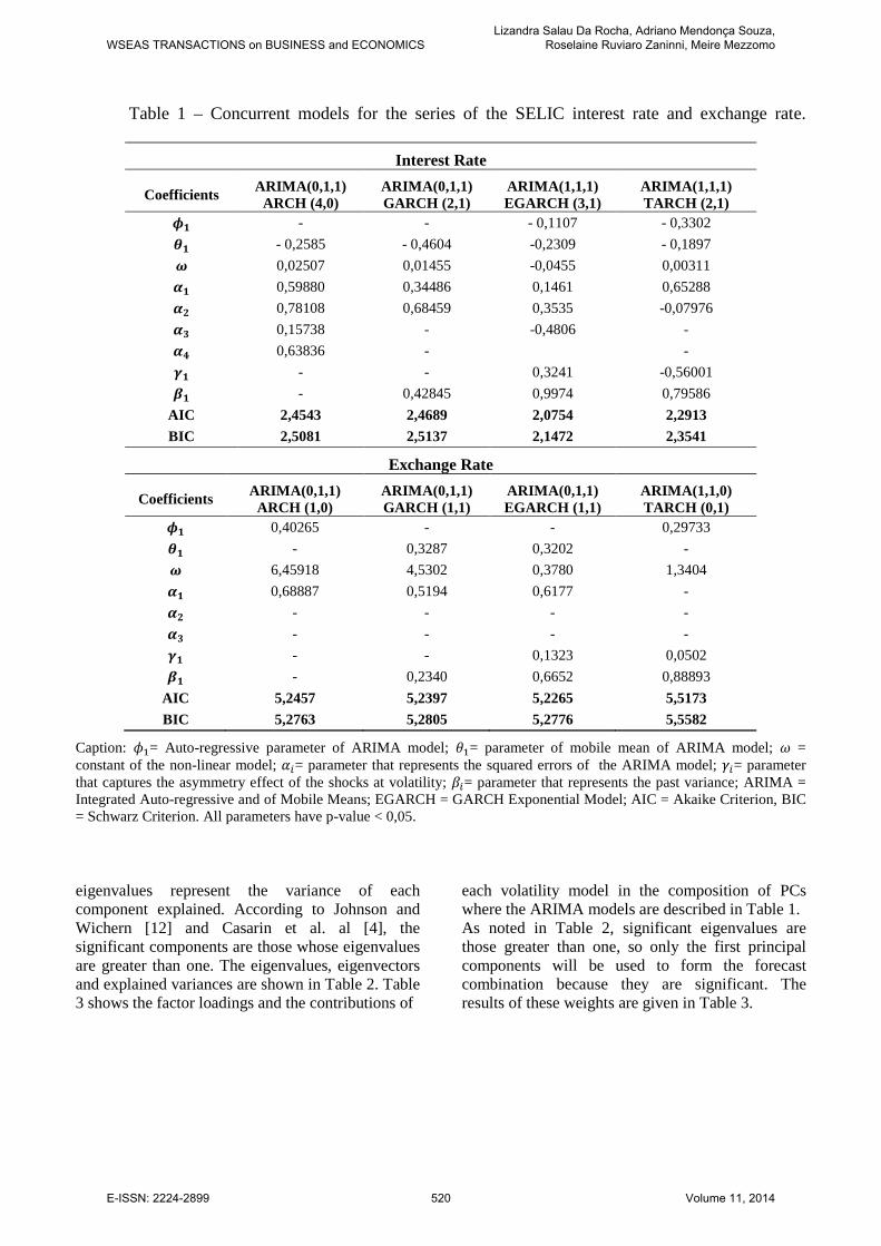
Table 1 – Concurrent models for the series of the SELIC interest rate and exchange rate.

Interest Rate

Coefficients ARIMA(0,1,1) ARCH (4,0)

ARIMA(0,1,1) GARCH (2,1)

ARIMA(1,1,1) EGARCH (3,1)

ARIMA(1,1,1) TARCH (2,1)

- - - 0,1107 - 0,3302 - 0,2585 - 0,4604 -0,2309 - 0,1897 0,02507 0,01455 -0,0455 0,00311 0,59880 0,34486 0,1461 0,65288 0,78108 0,68459 0,3535 -0,07976 0,15738 - -0,4806 - 0,63836 - - - - 0,3241 -0,56001 - 0,42845 0,9974 0,79586

AIC 2,4543 2,4689 2,0754 2,2913 BIC 2,5081 2,5137 2,1472 2,3541

Exchange Rate

Coefficients ARIMA(0,1,1) ARCH (1,0)

ARIMA(0,1,1) GARCH (1,1)

ARIMA(0,1,1) EGARCH (1,1)

ARIMA(1,1,0) TARCH (0,1)

0,40265 - - 0,29733 - 0,3287 0,3202 - 6,45918 4,5302 0,3780 1,3404 0,68887 0,5194 0,6177 - - - - - - - - - - - 0,1323 0,0502 - 0,2340 0,6652 0,88893

AIC 5,2457 5,2397 5,2265 5,5173 BIC 5,2763 5,2805 5,2776 5,5582

Caption: = Auto-regressive parameter of ARIMA model; = parameter of mobile mean of ARIMA model; = constant of the non-linear model; = parameter that represents the squared errors of the ARIMA model; = parameter that captures the asymmetry effect of the shocks at volatility; = parameter that represents the past variance; ARIMA = Integrated Auto-regressive and of Mobile Means; EGARCH = GARCH Exponential Model; AIC = Akaike Criterion, BIC = Schwarz Criterion. All parameters have p-value < 0,05. eigenvalues represent the variance of each component explained. According to Johnson and Wichern [12] and Casarin et al. al [4], the significant components are those whose eigenvalues are greater than one. The eigenvalues, eigenvectors and explained variances are shown in Table 2. Table 3 shows the factor loadings and the contributions of

each volatility model in the composition of PCs where the ARIMA models are described in Table 1. As noted in Table 2, significant eigenvalues are those greater than one, so only the first principal components will be used to form the forecast combination because they are significant. The results of these weights are given in Table 3.



E-ISSN: 2224-2899 520 Volume 11, 2014

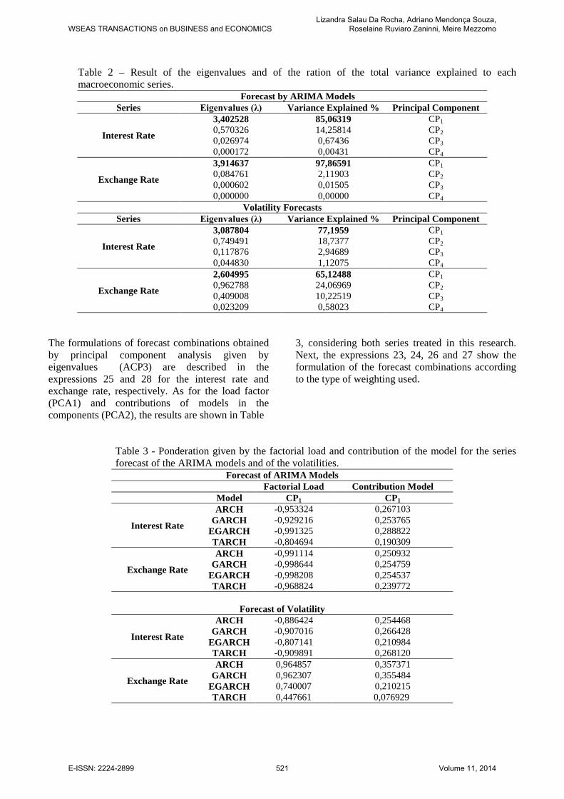
Table 2 – Result of the eigenvalues and of the ration of the total variance explained to each macroeconomic series.

Forecast by ARIMA Models Series Eigenvalues (λ) Variance Explained % Principal Component

Interest Rate

3,402528 85,06319 CP1 0,570326 14,25814 CP2 0,026974 0,67436 CP3 0,000172 0,00431 CP4

Exchange Rate

3,914637 97,86591 CP1 0,084761 2,11903 CP2 0,000602 0,01505 CP3 0,000000 0,00000 CP4

Volatility Forecasts Series Eigenvalues (λ) Variance Explained % Principal Component

Interest Rate

3,087804 77,1959 CP1 0,749491 18,7377 CP2 0,117876 2,94689 CP3 0,044830 1,12075 CP4

Exchange Rate

2,604995 65,12488 CP1 0,962788 24,06969 CP2 0,409008 10,22519 CP3 0,023209 0,58023 CP4

The formulations of forecast combinations obtained by principal component analysis given by eigenvalues (ACP3) are described in the expressions 25 and 28 for the interest rate and exchange rate, respectively. As for the load factor (PCA1) and contributions of models in the components (PCA2), the results are shown in Table

3, considering both series treated in this research. Next, the expressions 23, 24, 26 and 27 show the formulation of the forecast combinations according to the type of weighting used.

Table 3 - Ponderation given by the factorial load and contribution of the model for the series forecast of the ARIMA models and of the volatilities.

Forecast of ARIMA Models

Factorial Load Contribution Model

Model CP1 CP1

Interest Rate

ARCH -0,953324 0,267103 GARCH -0,929216 0,253765

EGARCH -0,991325 0,288822 TARCH -0,804694 0,190309

Exchange Rate

ARCH -0,991114 0,250932 GARCH -0,998644 0,254759

EGARCH -0,998208 0,254537 TARCH -0,968824 0,239772

Forecast of Volatility

Interest Rate

ARCH -0,886424 0,254468 GARCH -0,907016 0,266428

EGARCH -0,807141 0,210984 TARCH -0,909891 0,268120

Exchange Rate

ARCH 0,964857 0,357371 GARCH 0,962307 0,355484

EGARCH 0,740007 0,210215 TARCH 0,447661 0,076929



E-ISSN: 2224-2899 521 Volume 11, 2014

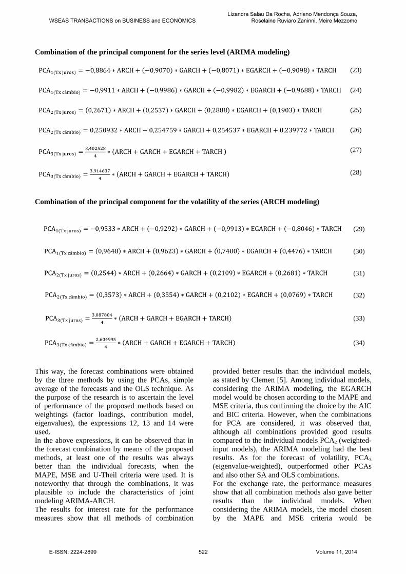
Combination of the principal component for the series level (ARIMA modeling)

(23)

(24)

(25)

(26)

(27)

(28)

Combination of the principal component for the volatility of the series (ARCH modeling)

(29)

(30)

(31)

(32)

(33)

(34)

This way, the forecast combinations were obtained by the three methods by using the PCAs, simple average of the forecasts and the OLS technique. As the purpose of the research is to ascertain the level of performance of the proposed methods based on weightings (factor loadings, contribution model, eigenvalues), the expressions 12, 13 and 14 were used. In the above expressions, it can be observed that in the forecast combination by means of the proposed methods, at least one of the results was always better than the individual forecasts, when the MAPE, MSE and U-Theil criteria were used. It is noteworthy that through the combinations, it was plausible to include the characteristics of joint modeling ARIMA-ARCH. The results for interest rate for the performance measures show that all methods of combination

provided better results than the individual models, as stated by Clemen [5]. Among individual models, considering the ARIMA modeling, the EGARCH model would be chosen according to the MAPE and MSE criteria, thus confirming the choice by the AIC and BIC criteria. However, when the combinations for PCA are considered, it was observed that, although all combinations provided good results compared to the individual models PCA2 (weighted-input models), the ARIMA modeling had the best results. As for the forecast of volatility, PCA3 (eigenvalue-weighted), outperformed other PCAs and also other SA and OLS combinations. For the exchange rate, the performance measures show that all combination methods also gave better results than the individual models. When considering the ARIMA models, the model chosen by the MAPE and MSE criteria would be



E-ISSN: 2224-2899 522 Volume 11, 2014

THARCH, while the AIC and BIC criteria would choose EGARCH. When considering the combinations of PCA, it is found that PCA3 (eigenvalue-weighted) had the best results for the ARIMA models. Between the performance measures for the volatility forecasts, PCA1 (weighting-factor loading) performed better compared to other PCAs and also the other SM and OLS combinations. Therefore, it is important to use more than one combination of principal components, considering various weight factors to check which one can better fit the models when performance indicators are considered. As evidenced by the results, the forecast combinations provide better results by allowing the relevant characteristics of each concurrent model to be taken into account, contrary to forecasts by an individual model. Thus, it is feasible to obtain better forecasts for the series under study. This means that this methodology can be applied to any type of time series. 6 Conclusion This paper sought to evaluate different volatility models for the SELIC interest rate and the Brazilian exchange rate to verify, by means of performance measures, which models would achieve better results. The individual models adopted were ARCH, GARCH, EGARCH and THARCH, plus three forecast combination methods (PCA, SA and OLS), where three different weights were considered for the PCA technique, resulting in five forecast combinations. The MAPE, MSE and U-THEIL criteria were used to evaluate the performance of the models and combinations. The forecast results show that, in general, the combination techniques produce better results than the individual models for the two series (interest rate and exchange rate). Considering the PCA combination techniques for the interest rate for the ARIMA forecasts, PCA2 outperformed other PCs, and the OLS combination technique had the worst performance. The best and worst performance for the volatility forecasts were PCA3 and OLS, respectively. For the exchange rate, the best performance was given by PCA3 when the ARIMA models are considered, and by PCA1for volatility, while OLS produced the worst measures. Thus, it is relevant to use more than one type of combination, in addition to considering more than one weight factor for the combination by Principal Component Analysis. A suggestion for future research is the comparison with other forecasting models such as VAR-VEC

models, econometric models, among others, comparing them with time-series models, and use other techniques such as moving average combination. ACKNOWLEDGEMENTS We would like to thank to Brazilian National Council for Scientific and Technological Development (CNPQ) for partially supporting this research, and for the anonymous references for their valuables contributions. References: [1] BOLLERSLEV,T., Generalized autoregressive

conditional heteroscedasticity. Journal of Econometrics, Vol. 31, 1986.

[2] BUENO, R. L. S., Econometria de Séries Temporais. São Paulo: Cengage Learning, 2008.

[3] BUENO, R. L. S., Econometria de Séries Temporais. São Paulo: Cengage Learning, 2012.

[4] CASARIN, V. A. et al., Continuous casting process stability evaluated by means of residuals control charts in the presence of cross-correlation and autocorrelation. International Journal of Academic Research, Vol. 4, No. 3, 2012.

[5] CLEMEN, R.T., Combining forecasts: a review and annotated bibliography. International Journal of Forecasting, Vol.5, 1989.

[6] DIEBOLD, F. X.; LOPEZ, J. A., Forecast evaluation and combination. In: NB ER Working Paper n. T0192. Available at: http://ssrn.com/abstract=225136, Mar, 1996.

[7] ENGLE, R. F. Autoregressive conditional heteroscedasticity with estimates of the variance of United Kingdom inflation. Econometrica, Vol. 50, 1982, pp.987- 1007.

[8] FERREIRA N. B.; MENEZES RUI, MENDES, D. A. Asymmetric conditional volatility in international stock markets. Phisica A, Vol. 382, 2007.

[9] GUPTA, S.; WILTON, P. C. Combination of Forecasts: Na Extension. Management Sience, Vol. 13, No. 3, 1977.

[10] JACKSON, J.E. Principal components and factor analysis: Part I – principal components. Journal of Quality Technology, October. Vol.12, No.4, 1981.

[11] JACKSON, J.E. Principal components and factor analysis: Part II – additional topics related to principal components. Journal of



E-ISSN: 2224-2899 523 Volume 11, 2014

http://ssrn.com/abstract=225136

Quality Technology, January, Vol.13. No.1, 1981.

[12] JOHNSON, R.A., WICHERN, D.W. Applied multivariate statistical analysis. Prentice-Hall. New Jersey, 1992.

[13] HOTTELLING, H. Analysis of a complex of Statistical variables into principal components. The Journal of Educational Psychology, Vol.24, 1933.

[14] LIBBLY, R. e BLASHFIELD, R.K, Performance of a Composite as a Function of Number of Judges. Organizacional Behavior and human Performance, Vol. 21, 1978.

[15] NELSON, B. Daniel., Conditional Heteroscedasticity in Asset Returns: A New Approach. Econometrica, Vol. 59, 1991.

[16] MAKRIDAKIS, S.G.;WINKLER, R.L. Averages of forecasts: some empirical results. Maganament Science. Vol.29, No. 9, 1983.

[17] MORRISON, D.F, Multivariate statistical methods. 2. Ed., New York, NY. Mc Graw Hill, 1976.

[18] PEARSON, K. On lines and planes of closed fit to system of point in space. Philosophical. Magazine, Vol. 6, 1901.

[19] RAUSSER, G.C.; OLIVEIRA, R. A., An econometric analysis of wilerness area use. Journal of the American Statical Association, Vol.71, No. 354, 1976.

[20] REINSEL, G. C, Elements of multivariate time series analysis. Springer-Verlag. New York, 1993.

[21] REIS, E. Estatística Multivariada Aplicada. Edições. Sílabo, 2001.

[22] SEBER, G.A.F, Multivariate observation. Wiley Series in Probability and Mathematical Statistics. John Wiley and Sons, Inc. NY, 1984.

[23] SOUZA, M. A.; SOUZA, M. F.; MENEZES, R. Procedure to evaluate multivariate statistical process control using ARIMA-ARCH models. Japan Industrial Management Association, Vol. 63, 2012.

[24] TSAY, S. RUEY. Analysis of Financial Time Series. New Jersey: John Wiley & Sons, Inc., Hoboken, 2005.

[25] WERNER, L. Um modelo Composto para realizar previsão de demanda através da integração da Combinação de previsões e do ajuste baseado na opinião. Tese de Doutorado do Curso de Pós-Graduação em Engenharia de Produção da Universidade Federal do Rio Grande do Sul, 2004.

[26] ZAKOIAN, J.M. Threshold Heteroskedasticity Models. Journal of Economic Dynamics and Control, Vol.18, 1994, pp. 931-955.



E-ISSN: 2224-2899 524 Volume 11, 2014

volatility forecast combination of brazilian selic ... · volatility forecast combination of...

Documents