EUROPEAN UNIVERSITY INSTITUTEDEPARTMENT OF ECONOMICS

EUI Working Paper ECO No. 2004/8

Residual Autocorrelation Testing

for Vector Error Correction Models

RALF BRÜGGERMANN, HELMUT LÜTKEPOHL

and

PENTTI SAIKKONEN

BADIA FIESOLANA, SAN DOMENICO (FI)

All rights reserved.No part of this paper may be reproduced inany form

Without permission of the author(s).

©2004 Ralf Brüggermann, Helmut Lütkepohl and Pentti SaikkonenPublished in Italy in January 2004

European University InstituteBadia Fiesolana

I-50016 San Domenico (FI)Italy

*Revisions of this work can be found at: http://www.iue.it/Personal/Luetkepohl/

January 8, 2004

Residual Autocorrelation Testing for Vector Error

Correction Models 1

Ralf Bruggemann

European University Institute, Florence and Humboldt University, Berlin

Helmut Lutkepohl

European University Institute, Florence and Humboldt University, Berlin

Pentti Saikkonen

University of Helsinki

Address for correspondence: Helmut Lutkepohl, Economics Department, European Univer-

sity Institute, Via della Piazzuola 43, I-50133 Firenze, ITALY

email: helmut.luetkepohl@iue.it

Abstract

In applied time series analysis, checking for autocorrelation in a fitted model is a routine

diagnostic tool. Therefore it is useful to know the asymptotic and small sample properties

of the standard tests for the case when some of the variables are cointegrated. The prop-

erties of residual autocorrelations of vector error correction models (VECMs) and tests for

residual autocorrelation are derived. In particular, the asymptotic distributions of Lagrange

multiplier (LM) and portmanteau tests are given. Monte Carlo simulations show that the

LM tests have advantages if autocorrelation of small order is tested whereas portmanteau

tests are preferable for higher order residual autocorrelation. Their critical values have to

be adjusted for the cointegration rank of the system, however.

JEL classification: C32

Keywords: Cointegration, dynamic econometric models, vector autoregressions, vector error

correction models, residual autocorrelation

1The third author thanks the Yrjo Jahnsson Foundation, the Academy of Finland and the Alexander vonHumboldt Foundation under a Humboldt research award for financial support. Part of this research wasdone while he was visiting the European University Institute in Florence.

1

1 Introduction

When a model for the data generation process (DGP) of a time series or a set of time series

has been constructed, it is common to perform checks of the model adequacy. Tests for

residual autocorrelation (AC) are prominent tools for this task. A number of such tests

are in routine use for both stationary as well as nonstationary processes with integrated or

cointegrated variables. Well-known examples are portmanteau and Lagrange multiplier (LM)

tests for residual AC. They are, for example, available in commercial econometric software

such as EViews and PcGive. The theoretical properties of these tests are well explored for

stationary DGPs (see, e.g., Ahn (1988), Hosking (1980, 1981a, 1981b), Li & McLeod (1981)

or Lutkepohl (1991) for a textbook exposition with more references and Edgerton & Shukur

(1999) for a large scale small sample comparison of various tests). An explicit treatment of

the properties of residual ACs of vector error correction models (VECMs) for cointegrated

variables does not seem to be available, however. This may also be the reason why no

critical values or p-values are presented in PcGive for some AC tests for VECMs. On the

other hand, p-values based on the asymptotic distributions of portmanteau and LM tests for

AC are provided in EViews 4 although a theoretical justification seems to be missing. In

fact, it will be seen from our results that the degrees of freedom of the portmanteau tests

should be adjusted in the presence of cointegration.

In this study it will be assumed that all variables are stationary or integrated of order one

(I(1)) and the DGP is a VECM with cointegration rank r. The asymptotic distribution of

the residual ACs is derived for a model estimated by reduced rank (RR) regression or some

similar method. The crucial condition here is that the cointegration matrix is estimated

superconsistently. In that case it turns out that the residual ACs have the same asymptotic

distribution as if the cointegration relations were known. There may also be restrictions on

the cointegration or short-run parameters.

Because standard tests for residual AC are based on the estimated autocovariances or

ACs, the asymptotic properties of the tests follow from those of these quantities. In partic-

ular, we consider LM tests and portmanteau tests in more detail. While the former tests

have the same asymptotic distribution as in the stationary case, the situation is different

for the portmanteau tests. For the latter tests the degrees of freedom have to be adjusted

to account for the cointegration rank of the system. Thus, the practice used in EViews 4,

2

for example, to subtract only the number of parameters associated with differenced lagged

values from the number of autocorrelations included in the statistic when determining the

degrees of freedom, has no asymptotic justification.

We also analyze the small sample properties of the tests in a Monte Carlo study. Not

surprisingly, some of the tests have small sample properties for which the asymptotic theory

is a poor guide. Similar results have also been found for stationary processes (Edgerton &

Shukur (1999) and Doornik (1996)). It turns out, however, that for low-dimensional systems

and moderately large samples, the usual tests perform reasonably well if the cointegration

properties of the process are taken into account properly.

The study is organized as follows. In the next section the model setup is presented and

the asymptotic properties of the residual autocovariances and ACs are discussed in Section

3. Tests for residual AC are considered in Section 4. The results of a Monte Carlo study are

presented in Section 5 and concluding remarks follow in Section 6. Proofs are presented in

the Appendix.

The following general notation will be used. The differencing and lag operators are

denoted by ∆ and L, respectively. Convergence in distribution is signified byd→ and log

denotes the natural logarithm. Op(·) and op(·) are the usual symbols for boundedness in

probability. Independently, identically distributed is abbreviated by iid. The trace, deter-

minant and rank of the matrix A are denoted by tr(A), det(A) and rk(A), respectively. The

symbol vec is used for the column vectorization operator. If A is an (n × m) matrix of

full column rank (n > m), we denote an orthogonal complement by A⊥. The orthogonal

complement of a nonsingular square matrix is zero and the orthogonal complement of a zero

matrix is an identity matrix of suitable dimension. An (n×n) identity matrix is denoted by

In. DGP, ML, LS, GLS, RR, LR and LM are used to abbreviate data generation process,

maximum likelihood, least squares, generalized least squares, reduced rank, likelihood ratio

and Lagrange multiplier, respectively. VAR and VECM stand for vector autoregression and

vector error correction model, respectively. A sum is defined to be zero if the lower bound

of the summation index exceeds the upper bound.

3

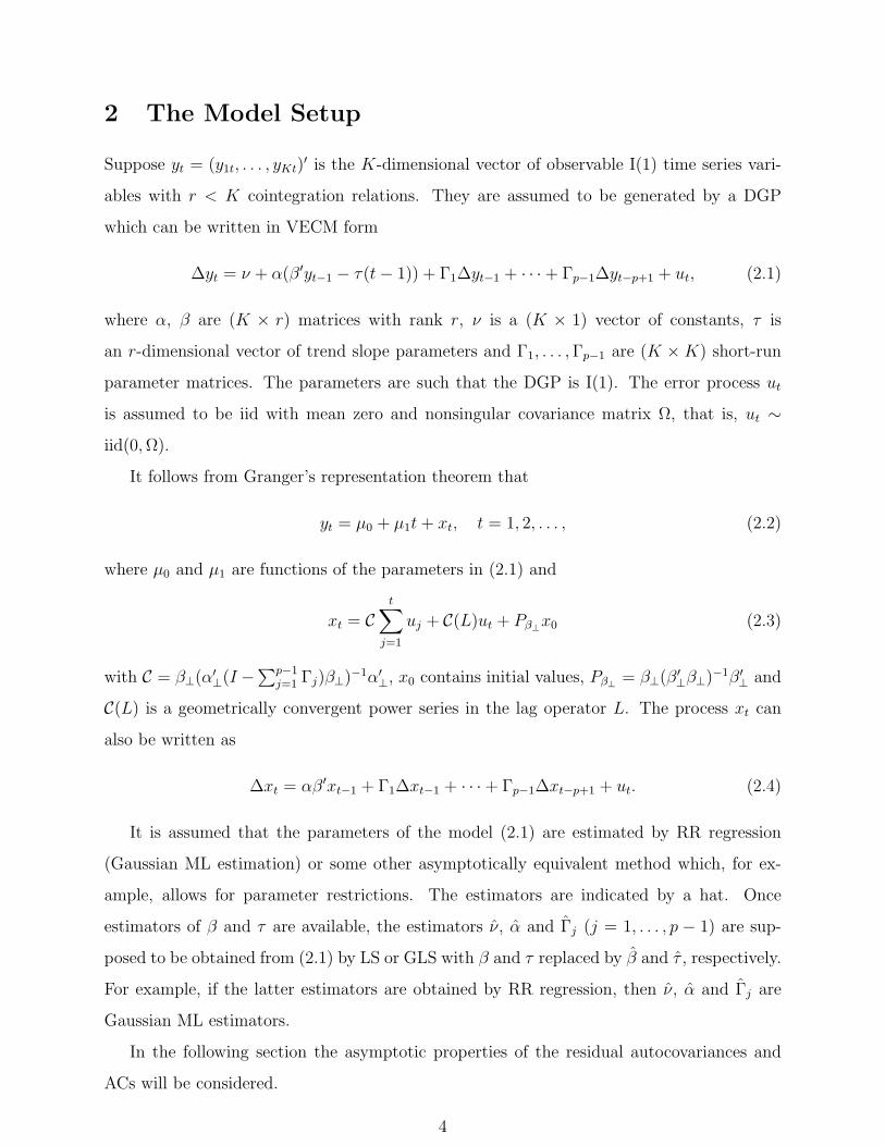
2 The Model Setup

Suppose yt = (y1t, . . . , yKt)′ is the K-dimensional vector of observable I(1) time series vari-

ables with r < K cointegration relations. They are assumed to be generated by a DGP

which can be written in VECM form

∆yt = ν + α(β′yt−1 − τ(t− 1)) + Γ1∆yt−1 + · · ·+ Γp−1∆yt−p+1 + ut, (2.1)

where α, β are (K × r) matrices with rank r, ν is a (K × 1) vector of constants, τ is

an r-dimensional vector of trend slope parameters and Γ1, . . . , Γp−1 are (K ×K) short-run

parameter matrices. The parameters are such that the DGP is I(1). The error process ut

is assumed to be iid with mean zero and nonsingular covariance matrix Ω, that is, ut ∼iid(0, Ω).

It follows from Granger’s representation theorem that

yt = µ0 + µ1t + xt, t = 1, 2, . . . , (2.2)

where µ0 and µ1 are functions of the parameters in (2.1) and

xt = Ct∑

j=1

uj + C(L)ut + Pβ⊥x0 (2.3)

with C = β⊥(α′⊥(I −∑p−1j=1 Γj)β⊥)−1α′⊥, x0 contains initial values, Pβ⊥ = β⊥(β′⊥β⊥)−1β′⊥ and

C(L) is a geometrically convergent power series in the lag operator L. The process xt can

also be written as

∆xt = αβ′xt−1 + Γ1∆xt−1 + · · ·+ Γp−1∆xt−p+1 + ut. (2.4)

It is assumed that the parameters of the model (2.1) are estimated by RR regression

(Gaussian ML estimation) or some other asymptotically equivalent method which, for ex-

ample, allows for parameter restrictions. The estimators are indicated by a hat. Once

estimators of β and τ are available, the estimators ν, α and Γj (j = 1, . . . , p − 1) are sup-

posed to be obtained from (2.1) by LS or GLS with β and τ replaced by β and τ , respectively.

For example, if the latter estimators are obtained by RR regression, then ν, α and Γj are

Gaussian ML estimators.

In the following section the asymptotic properties of the residual autocovariances and

ACs will be considered.

4

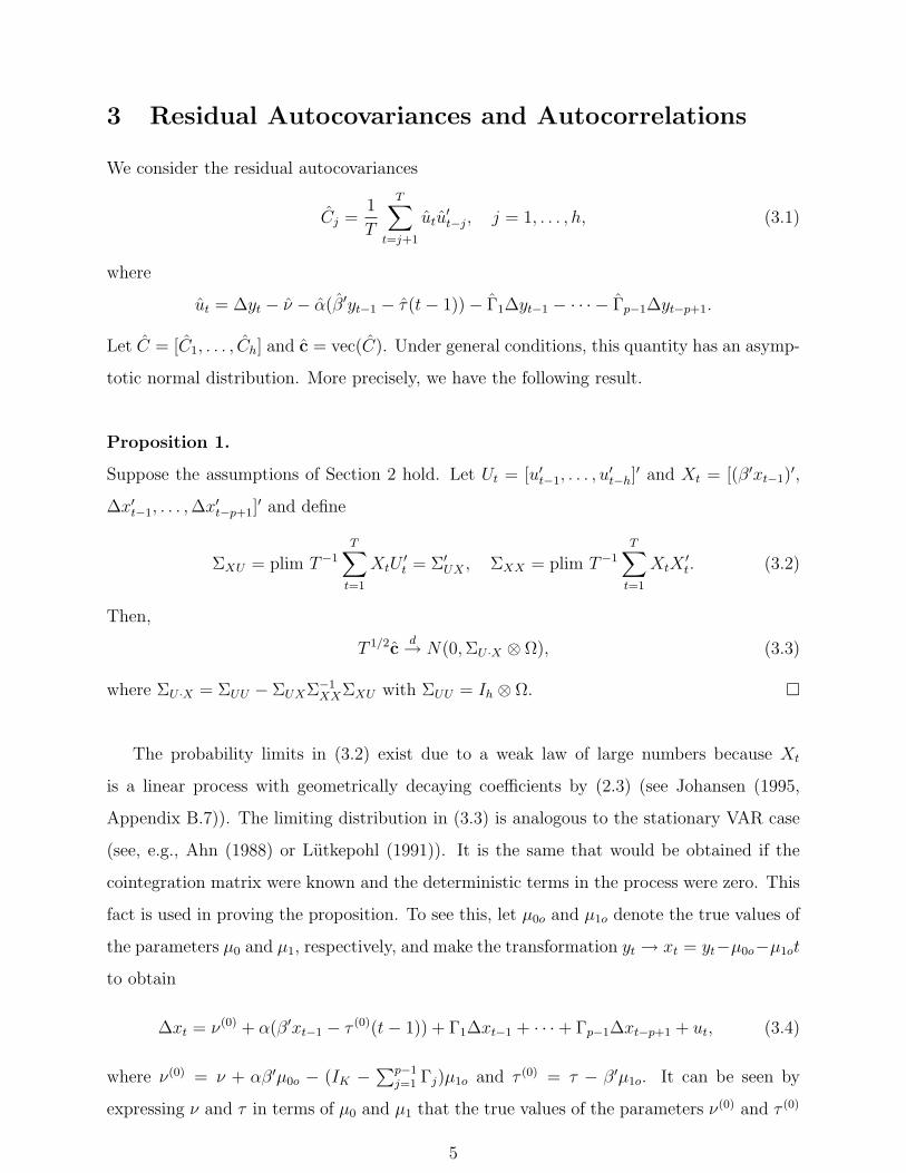
3 Residual Autocovariances and Autocorrelations

We consider the residual autocovariances

Cj =1

T

T∑t=j+1

utu′t−j, j = 1, . . . , h, (3.1)

where

ut = ∆yt − ν − α(β′yt−1 − τ(t− 1))− Γ1∆yt−1 − · · · − Γp−1∆yt−p+1.

Let C = [C1, . . . , Ch] and c = vec(C). Under general conditions, this quantity has an asymp-

totic normal distribution. More precisely, we have the following result.

Proposition 1.

Suppose the assumptions of Section 2 hold. Let Ut = [u′t−1, . . . , u′t−h]

′ and Xt = [(β′xt−1)′,

∆x′t−1, . . . , ∆x′t−p+1]′ and define

ΣXU = plim T−1

T∑t=1

XtU′t = Σ′

UX , ΣXX = plim T−1

T∑t=1

XtX′t. (3.2)

Then,

T 1/2cd→ N(0, ΣU ·X ⊗ Ω), (3.3)

where ΣU ·X = ΣUU − ΣUXΣ−1XXΣXU with ΣUU = Ih ⊗ Ω. ¤

The probability limits in (3.2) exist due to a weak law of large numbers because Xt

is a linear process with geometrically decaying coefficients by (2.3) (see Johansen (1995,

Appendix B.7)). The limiting distribution in (3.3) is analogous to the stationary VAR case

(see, e.g., Ahn (1988) or Lutkepohl (1991)). It is the same that would be obtained if the

cointegration matrix were known and the deterministic terms in the process were zero. This

fact is used in proving the proposition. To see this, let µ0o and µ1o denote the true values of

the parameters µ0 and µ1, respectively, and make the transformation yt → xt = yt−µ0o−µ1ot

to obtain

∆xt = ν(0) + α(β′xt−1 − τ (0)(t− 1)) + Γ1∆xt−1 + · · ·+ Γp−1∆xt−p+1 + ut, (3.4)

where ν(0) = ν + αβ′µ0o − (IK − ∑p−1j=1 Γj)µ1o and τ (0) = τ − β′µ1o. It can be seen by

expressing ν and τ in terms of µ0 and µ1 that the true values of the parameters ν(0) and τ (0)

5

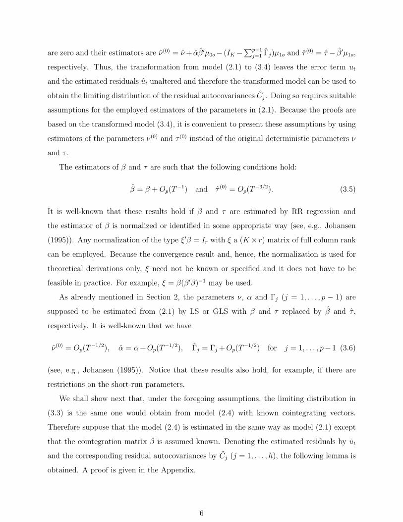
are zero and their estimators are ν(0) = ν + αβ′µ0o− (IK −∑p−1

j=1 Γj)µ1o and τ (0) = τ − β′µ1o,

respectively. Thus, the transformation from model (2.1) to (3.4) leaves the error term ut

and the estimated residuals ut unaltered and therefore the transformed model can be used to

obtain the limiting distribution of the residual autocovariances Cj. Doing so requires suitable

assumptions for the employed estimators of the parameters in (2.1). Because the proofs are

based on the transformed model (3.4), it is convenient to present these assumptions by using

estimators of the parameters ν(0) and τ (0) instead of the original deterministic parameters ν

and τ .

The estimators of β and τ are such that the following conditions hold:

β = β + Op(T−1) and τ (0) = Op(T

−3/2). (3.5)

It is well-known that these results hold if β and τ are estimated by RR regression and

the estimator of β is normalized or identified in some appropriate way (see, e.g., Johansen

(1995)). Any normalization of the type ξ′β = Ir with ξ a (K× r) matrix of full column rank

can be employed. Because the convergence result and, hence, the normalization is used for

theoretical derivations only, ξ need not be known or specified and it does not have to be

feasible in practice. For example, ξ = β(β′β)−1 may be used.

As already mentioned in Section 2, the parameters ν, α and Γj (j = 1, . . . , p − 1) are

supposed to be estimated from (2.1) by LS or GLS with β and τ replaced by β and τ ,

respectively. It is well-known that we have

ν(0) = Op(T−1/2), α = α+Op(T

−1/2), Γj = Γj +Op(T−1/2) for j = 1, . . . , p− 1 (3.6)

(see, e.g., Johansen (1995)). Notice that these results also hold, for example, if there are

restrictions on the short-run parameters.

We shall show next that, under the foregoing assumptions, the limiting distribution in

(3.3) is the same one would obtain from model (2.4) with known cointegrating vectors.

Therefore suppose that the model (2.4) is estimated in the same way as model (2.1) except

that the cointegration matrix β is assumed known. Denoting the estimated residuals by ut

and the corresponding residual autocovariances by Cj (j = 1, . . . , h), the following lemma is

obtained. A proof is given in the Appendix.

6

Lemma 1.

Cj − Cj = Op(T−1), j = 1, . . . , h. (3.7)

¤

A proof of Proposition 1 based on this lemma is also given in the Appendix. It follows

immediately from Proposition 1 that an analogous result also holds for the residual ACs.

Notice that the AC matrix corresponding to Cj is Rj = S−1CjS−1, where S is a diagonal

matrix with the square roots of the diagonal elements of Ω = T−1∑T

t=1 utu′t on the diag-

onal. Moreover, let S be the corresponding diagonal matrix with the square roots of the

diagonal elements of Ω on the diagonal and let R0 = S−1ΩS−1 be the correlation matrix

corresponding to Ω. With this notation we can state the following corollary of Proposition 1.

Corollary 1.

Let R = [R1, . . . , Rh] and r = vec(R) = (Ih ⊗ S−1 ⊗ S−1)c. Then, under the conditions of

Proposition 1,

T 1/2rd→ N(0, [(Ih ⊗ S−1)ΣU ·X(Ih ⊗ S−1)]⊗R0). (3.8)

¤

This result can be used to set up confidence intervals around zero for the residual ACs

of an estimated VECM in the same way as for stationary processes (see, e.g., Lutkepohl

(1991)). As in the latter case, the asymptotic standard errors are smaller than the crude

1/√

T approximations which are sometimes used as a rough check for residual AC. A couple

of extensions may be worth noting.

Extension 1. The results also hold if there is no deterministic trend term in the model.

In other words, τ = 0 is known a priori. Moreover, seasonal dummies may be added to the

model. They do not have an effect on the asymptotic distributions of the residual autoco-

variances and ACs.

Extension 2. There may be linear or smooth nonlinear restrictions on the parameters α

7

and Γj (j = 1, . . . , p− 1). Zero restrictions are, of course, a leading case of such restrictions.

Suppose that α = α(θ) and Γj = Γj(θ) (j = 1, . . . , p − 1) with θ an underlying structural

parameter. Suppose the estimator of θ is consistent and asymptotically normal. Then the

previous results continue to hold with the usual adjustments to the asymptotic covariance

matrix of the parameter estimators and, hence of ΣU ·X (see Ahn (1988) or Lutkepohl (1991)),

if the corresponding estimators of α and Γj satisfy (3.6) and the estimators of β and τ main-

tain their convergence rates and are asymptotically independent of the estimator of θ. It has

been discussed by Johansen (1991, Appendix) and Reinsel & Ahn (1992) that the required

asymptotic estimation theory holds for restricted versions of model (2.1). One restriction

of particular importance is obtained by confining the intercept term to the cointegration

relations. This constraint may be imposed if there are no linear deterministic trends in the

variables. It is considered by Saikkonen (2001a, b).

Extension 3. The same asymptotic distributions are also obtained for the residual autoco-

variances and ACs if the model (2.1) is estimated without the cointegration restriction, that

is, the cointegration rank r is ignored and no restriction is placed on the error correction

term. Instead of (2.1) we then consider

∆yt = ν + ν1(t− 1) + Πyt−1 + Γ1∆yt−1 + · · ·+ Γp−1∆yt−p+1 + ut, (3.9)

where ν1 = −ατ and Π = αβ′. The parameters are assumed to be estimated by LS and the

resulting estimators are again indicated by a hat. The error term ut and the LS residuals

ut are again invariant to subtracting the deterministic term so that the corresponding true

parameter values may be assumed to be zero and yt = xt can be assumed in (3.9). Using

further the transformation

Πxt−1 = αβ′[ξo : βo⊥]

β′o

ξ′o⊥

xt−1 = a(β′oxt−1) + b(ξ′o⊥xt−1),

where a = αβ′ξo, b = αβ′βo⊥ and ‘o’ refers to true parameter values, the limiting distribution

of the residual autocovariances can be derived by replacing (3.9) by

∆xt = ν(0) + ν(0)1 (t− 1) + av0t + bv1t + Γ1∆xt−1 + · · ·+ Γp−1∆xt−p+1 + ut, (3.10)

where v0t = β′oxt−1, v1t = ξ′o⊥xt−1, ν(0) is as defined before and ν(0)1 = −ατ (0) so that the true

values of the parameters ν(0), ν(0)1 and b are zero. The processes ∆xt and v0t are stationary

8

and have zero mean whereas v1t is I(1) and not cointegrated. The LS residuals ut from

(3.9) can be considered as LS residuals from (3.10). In the same way as in the proof of

Lemma 1, we can use well-known limit results of stationary and I(1) processes and obtain

an analog of Lemma 1 with Cj residual autocovariance matrices based on (3.10) and Cj LS

residual autocovariance matrices obtained from (3.10) with the constraints ν = 0, ν1 = 0

and b = 0 (see (A.2) in the Appendix). Thus, it suffices to obtain the limiting distribution

of Cj (j = 1, . . . , h) and Proposition 1 can be applied directly.

4 Testing for Residual Autocorrelation

Two types of tests for residual AC are quite popular in applied work, Breusch-Godfrey LM

tests and portmanteau tests. They are both based on statistics of the form

Q = T c′Σ−1c. (4.1)

where Σ is a suitable scaling matrix. In other words, they are based on the residual au-

tocovariances. The choice of scaling matrix Σ determines the type of test statistic and

its asymptotic distribution under the null hypothesis of no residual AC. For the Breusch-

Godfrey LM statistic, Σ is an estimator of the covariance matrix of the limiting distribution

in (3.3) of Proposition 1, whereas the portmanteau statistic uses an estimator of Ih⊗Ω⊗Ω

instead. We will consider both types of tests in turn.

4.1 Breusch-Godfrey Test

The Breusch-Godfrey test can be viewed as considering a VAR(h) model

ut = B1ut−1 + · · ·+ Bhut−h + εt (4.2)

for the error terms and testing the pair of hypotheses

H0 : B1 = · · · = Bh = 0 vs. H1 : B1 6= 0 or · · · or Bh 6= 0. (4.3)

For this purpose the auxiliary model

ut = B1ut−1 + · · ·+ Bhut−h + αβ∗′y∗t−1 + Γ1∆yt−1 + · · ·+ Γp−1∆yt−p+1

+ν + (y′t−1ξ⊥ ⊗ α)φ11 − α(t− 1)φ21 + et

= (U ′t ⊗ IK)γ + (Z ′

t ⊗ IK)φ + Z ′1tφ1 + et, t = 1, . . . , T,

(4.4)

9

may be used with β∗′ = [β′ : τ ], y∗t−1′ = [y′t−1 : t − 1], U ′

t = [u′t−1, . . . , u′t−h] (ut = 0 for

t ≤ 0), γ = vec[B1, . . . , Bh], Z ′t = [(β∗′y∗t−1)

′, ∆y′t−1, . . . , ∆y′t−p+1], φ = vec[α, Γ1, . . . , Γp−1],

Z ′1t = [IK : y′t−1ξ⊥ ⊗ α : −α(t − 1)] and φ′1 = [ν ′, φ′11, φ

′21]. The terms in Z1t are related to

the scores of ν, β and τ . Allowing for ν simply means including an intercept term in (4.4)

which is again denoted by ν for simplicity. Regarding β, the situation depends on a possible

normalization. If a normalization ξ′β = Ir with ξ known is used, the natural additional

regressor is y′t−1ξ⊥ ⊗ α. If a particular normalization is not used, the choice ξ⊥ = β⊥ can be

considered. The terms y′t−1ξ⊥ ⊗ α and −α(t− 1) may in fact be deleted from the auxiliary

model (see Remark 1 below).

The Breusch-Godfrey test statistic, say Q∗BG, is a standard LM test statistic for the null

hypothesis γ = 0 in (4.4),

Q∗BG = T γ′(Σγγ)−1γ = T c′(IhK ⊗ Ω−1)Σγγ(IhK ⊗ Ω−1)c, (4.5)

where γ is the GLS estimator of γ and Σγγ is the part of

T−1

T∑t=1

Ut ⊗ IK

Zt ⊗ IK

Z1t

Ω−1[U ′

t ⊗ IK : Z ′t ⊗ IK : Z ′

1t]

−1

corresponding to γ. That is,

Σγγ =(ΣUU −ΣUZΣ−1

ZZΣ′

UZ

)−1

with

ΣUU = T−1

T∑t=1

(Ut ⊗ IK)Ω−1(Ut ⊗ IK)′,

ΣUZ = T−1

T∑t=1

(Ut ⊗ IK)Ω−1[Z ′t ⊗ IK : Z ′

1t]

and

ΣZZ = T−1

T∑t=1

Zt ⊗ IK

Z1t

Ω−1[Z ′

t ⊗ IK : Z ′1t].

Here Ω = T−1∑T

t=1 utu′t as before and, hence, Ω is the residual covariance estimator from

the restricted auxiliary model (4.4). Because the scaling matrix used in (4.5) is a consistent

estimator of ΣU ·X ⊗ Ω, it follows immediately from Proposition 1 that

Q∗BG

d→ χ2(hK2).

10

Several remarks are worth making regarding this result.

Remark 1. Notice that the regressors y′t−1ξ⊥ ⊗ α and −α(t − 1) may be deleted from the

auxiliary model (4.4) without affecting the limiting distribution of the test. This result holds

because the estimators of β and τ are asymptotically independent of the estimators of γ and

φ. As far as the small sample properties of the test are concerned, it is not clear that deleting

these terms is a good idea because the independence does not hold in finite samples. We

will denote the statistic obtained from the auxiliary model without the regressors y′t−1ξ⊥⊗ α

and −α(t− 1) by QBG in the following. ¤

Remark 2. As mentioned in the previous section, Proposition 1 holds also if there are, for

example, seasonal dummies in the VECM (2.1). Because the limiting distribution of the LM

test statistics follows directly from the proposition, it is clear that the LM tests can also be

used to test for residual AC in models with seasonal dummies. In that case the seasonal

dummies should also be included in the auxiliary model (4.4). Also, from Extension 3 of

Proposition 1 it follows that Q∗BG has the same limiting null distribution if the cointegrating

rank is not taken into account and the model is estimated in unrestricted form. Equivalently,

the corresponding levels version may be estimated. ¤

Remark 3. There may be parameter restrictions on φ so that φ = φ(θ), as discussed in

Extension 2 in the previous section. Again, the limiting distributions of the LM statistics

are unaffected. Here the restrictions have to be taken into account in the auxiliary model in

the usual way, however. ¤

Remark 4. Rather than considering the full VAR(h) model (4.2) for the error term, a single

lag as in ut = Bhut−h + εt may be used in the alternative. In that case the null hypothesis is

H0 : Bh = 0. The relevant test statistic is obtained by replacing Ut with ut−h and considering

an auxiliary model just like (4.4) or the corresponding version without the terms y′t−1ξ⊥⊗ α

and −α(t − 1). In that case the limiting distribution of the LM statistic is χ2(K2). This

version of the test is, for example, given in EViews 4. ¤

11

Remark 5. It can be shown that the Breusch-Godfrey statistic can be written alternatively

as

QBG = T(K − tr(Ω−1Ωe)

),

where Ωe is the unrestricted residual covariance estimator of the auxiliary model used for

the test (see Edgerton & Shukur (1999)). Instead of using this LM version of the test

statistic, the asymptotically equivalent likelihood ratio (LR) or Wald versions may be used.

For example,

QLR = T (log det Ω− log det Ωe) (4.6)

or

QW = T(tr(Ω−1

e Ω)−K)

may be considered. The corresponding statistics based on the auxiliary model (4.4) with

regressors related to the scores of the cointegration parameters will be denoted by Q∗LR and

Q∗W , respectively. ¤

In the next subsection the portmanteau test will be discussed.

4.2 Portmanteau Test

Although portmanteau tests may also be regarded as tests for the pair of hypotheses in (4.3),

it may be more natural to think of them as tests for the null hypothesis

H0 : E(utu′t−i) = 0, i = 1, 2, . . . , (4.7)

which is tested against the alternative that at least one of these autocovariances and, hence,

one autocorrelation is nonzero. The basic form of the portmanteau test statistic is

QP = T

h∑j=1

tr(C ′jΩ

−1CjΩ−1) = T c′(Ih ⊗ Ω⊗ Ω)−1c. (4.8)

Appealing to Lemma 1, the limiting distribution of this statistic can be derived by using the

auxiliary regression model (2.4), with β treated as known. Transform xt to

zt = ξβ′xt + β⊥ξ′⊥∆xt

and define the lag polynomial matrix

D(L) = [Γ(L)ξ∆− αL : Γ(L)β⊥][β : ξ⊥]′,

12

where Γ(L) = IK −∑p−1

j=1 ΓjLj. Note that D(L) is of order p with D(L) = IK −

∑pj=1 DjL

j.

From Lemma 1 of Saikkonen (2003) and the subsequent discussion it follows that we can

transform model (2.4) to

zt =

p∑j=1

Djzt−j + ut. (4.9)

Note that this transformation does not affect the error term and that the process zt is station-

ary. Moreover, the parameter matrices D1, . . . , Dp are smooth functions of the parameters

α, Γ1, . . . , Γp−1 (see the definition of D(L) and recall that β (and ξ) are treated as known).

Using the LS estimators α, Γ1, . . . , Γp−1 of (2.4) one can obtain Gaussian ML estimators of

D1, . . . , Dp in an obvious way. The residuals ut can then be considered as residuals from a

Gaussian ML estimation of (4.9). Thus, we can conclude that the approximate distribution

of the portmanteau test can be obtained by applying the general result of Ahn (1988),

QP ≈ χ2(hK2 −K2(p− 1)−Kr)

in large samples if h is also large. Notice that due to the restrictions in the Dj parameter

matrices the degrees of freedom are different than for a stationary VAR(p) model where the

degrees of freedom are hK2 −K2p (e.g., Lutkepohl (1991)).

A related statistic with potentially superior small sample properties is the adjusted port-

manteau statistic,

Q∗P = T 2

h∑j=1

1

T − jtr(C ′

jC−10 CjC

−10 ),

(see, e.g., Hosking (1980)). Its asymptotic properties are the same as those of QP . A

number of other small sample adjustments with equivalent asymptotic properties have also

been considered in the literature for stationary models (e.g., Li & McLeod (1981), Johansen

(1995, p. 21/22)). They could be used for the presently considered case of cointegrated

processes as well.

If there are parameter restrictions for α, Γ1, . . . , Γp−1 the limiting theory still holds. How-

ever, the test statistics have approximate χ2(df) distributions, where the degrees of freedom

df = hK2− #freely estimated parameters in α and Γj, j = 1, . . . , p− 1.

13

5 Simulations

We check the small sample properties of the residual AC tests by using Monte Carlo simu-

lations because earlier studies for stationary processes (see Doornik (1996) and Edgerton &

Shukur (1999)) have shown that some tests have poor small sample properties and relying

on their asymptotic properties may be quite misleading. We therefore investigate the small

sample properties of different test variants discussed in Section 4 in the context of VECMs.

In particular, we consider the two variants of the LM tests, Q∗BG and QBG, as well as the

related LR and Wald versions of the BG test in our Monte Carlo study and compare their

properties. Moreover, the portmanteau tests, QP and Q∗P from Section 4.2 are considered.

The objective of our simulations is to see how the test versions considered in the previous

section perform in small samples when they are applied to cointegrated processes. It is

not our intension to provide a full scale investigation of all potential modifications of the

statistics that have been proposed for stationary processes.

5.1 Monte Carlo Design

Our Monte Carlo experiments are based on the following DGP specification

∆yt = ν + α(β′yt−1 − τ(t− 1)) + Γ1∆yt−1 + ut. (5.1)

Using this DGP structure a number of experiments have been conducted varying factors that

are likely to influence the small sample performance of different AC tests. In particular, we

change the dimension of the system (K = 2, . . . , 5), the cointegration rank (r = 1, . . . , K−1),

the parameters of the loading coefficients α, the dynamic structure Γ1 and the structure of

the error covariance matrix. Instead of reporting all Monte Carlo results we present a few

typical results in Section 5.2. Most of the results will be illustrated using a variant of the 3-

dimensional DGP (a) from Table 1. The cointegration matrix β of this DGP contains typical

(1,−1) relations, which are loaded into some of the VECM equations by the parameters a1.

The dynamic correlation structure given by Γ1 can be controlled by setting γ and γ1 as

in Edgerton & Shukur (1999). Trend term and intercept parameters are set by τ and ν,

respectively. Cross-equation error correlation is given by ρ, whereas the AC structure of

the error ut can be controlled by the parameters π1 and π2. The effects of increasing the

14

dimension is illustrated by using the 5-dimensional DGP (b) from Table 1. We give the

actual parameter values for different experiments in Table 2.

For each DGP variant given in Table 2 we have simulated M = 1000 sets of time series

data for yt using the levels version of (5.1) such that T = 50, 100, 200, 500, 1000 observations

can be used for estimation of the VECM model. We use the Johansen RR regression on

a VAR with correct lag length p = 2 and obtain an estimate of β and τ using the correct

rank restriction r. This estimate is used to setup a VECM for obtaining the residuals used

in AC testing. In each Monte Carlo replication we have applied the QBG, QLR, and QW

tests, the variants with cointegration terms (y′t−1ξ⊥ ⊗ α and −α(t − 1)) in the auxiliary

regression (Q∗BG, Q∗

LR, and Q∗W ) and both variants of the portmanteau test (QP and Q∗

P ) to

the residuals of the VECM. To investigate the size and power properties of the tests we have

recorded the relative rejection frequencies for different values of h. Results of the Monte

Carlo study will be discussed in the following subsection.

5.2 Monte Carlo Results

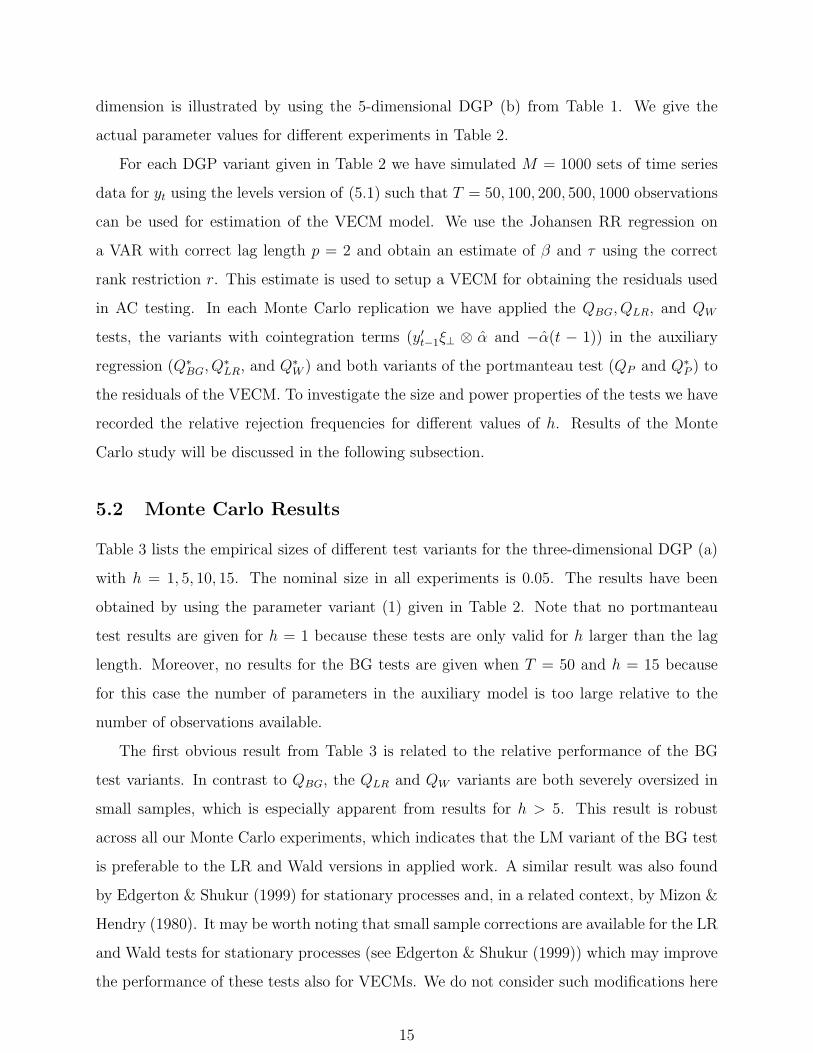
Table 3 lists the empirical sizes of different test variants for the three-dimensional DGP (a)

with h = 1, 5, 10, 15. The nominal size in all experiments is 0.05. The results have been

obtained by using the parameter variant (1) given in Table 2. Note that no portmanteau

test results are given for h = 1 because these tests are only valid for h larger than the lag

length. Moreover, no results for the BG tests are given when T = 50 and h = 15 because

for this case the number of parameters in the auxiliary model is too large relative to the

number of observations available.

The first obvious result from Table 3 is related to the relative performance of the BG

test variants. In contrast to QBG, the QLR and QW variants are both severely oversized in

small samples, which is especially apparent from results for h > 5. This result is robust

across all our Monte Carlo experiments, which indicates that the LM variant of the BG test

is preferable to the LR and Wald versions in applied work. A similar result was also found

by Edgerton & Shukur (1999) for stationary processes and, in a related context, by Mizon &

Hendry (1980). It may be worth noting that small sample corrections are available for the LR

and Wald tests for stationary processes (see Edgerton & Shukur (1999)) which may improve

the performance of these tests also for VECMs. We do not consider such modifications here

15

because Edgerton & Shukur (1999) find that they only partially correct the size distortions

in stationary systems.

Comparing results for QBG with those for Q∗BG reveals that including (y′t−1ξ⊥ ⊗ α) and

−α(t − 1)) in the auxiliary regression is not advantageous in small sample situations. On

the contrary, the variant without these additional terms typically outperforms Q∗BG in the

sense that its size is closer to the nominal size of the test. With the exception of T = 50,

the QBG variant has a size reasonably close to the nominal level of 5%.

Not surprisingly, the portmanteau test variants are oversized for h = 5, emphasizing

that they are only valid when h is considerably larger than the lag length of the model.

Accordingly, the size decreases when lags up to h = 10 or h = 15 are used. When using

a sufficiently large number of lags, we find the standard portmanteau statistic QP to have

an empirical size smaller than the nominal one (see Panels (c) and (d) of Table 3) in small

samples which is in line with earlier results for stationary processes (e.g., Hosking (1980))

and was the reason for proposing the adjusted statistic in the first place. In contrast, the

modified statistic Q∗P typically has size close to the nominal level for large h. Results from

Panels (b) through (d) suggest that the size of Q∗P decreases with increasing h. Therefore,

we also checked results for Q∗P with h = 20 and found that the size did not drop significantly

below the nominal level. Overall, the results for the portmanteau tests suggest that Q∗P

works better than QP in models with sample sizes common in applied work.

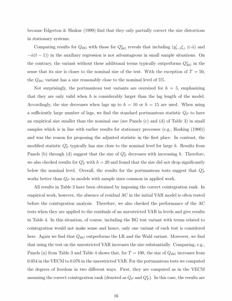
All results in Table 3 have been obtained by imposing the correct cointegration rank. In

empirical work, however, the absence of residual AC in the initial VAR model is often tested

before the cointegration analysis. Therefore, we also checked the performance of the AC

tests when they are applied to the residuals of an unrestricted VAR in levels and give results

in Table 4. In this situation, of course, including the BG test variant with terms related to

cointegration would not make sense and hence, only one variant of each test is considered

here. Again we find that QBG outperforms the LR and the Wald variant. Moreover, we find

that using the test on the unrestricted VAR increases the size substantially. Comparing, e.g.,

Panels (a) from Table 3 and Table 4 shows that, for T = 100, the size of QBG increases from

0.054 in the VECM to 0.076 in the unrestricted VAR. For the portmanteau tests we computed

the degrees of freedom in two different ways. First, they are computed as in the VECM

assuming the correct cointegration rank (denoted as QP and Q∗P ). In this case, the results are

16

similar to estimating the VECM. Second, the degrees of freedom are calculated based on the

usual formula for unrestricted VAR models (denoted as QV AR−DFP and Q∗,V AR−DF

P ). Doing

so almost doubles the size of the portmanteau tests. In other words, using the information

on the cointegration properties is important for the portmanteau tests. As a consequence,

an uncritical application of the portmanteau tests to a levels VAR is problematic if there are

integrated and possibly cointegrated variables. In that case, a VECM should be specified

and then the tests should be applied or the BG tests should be used.

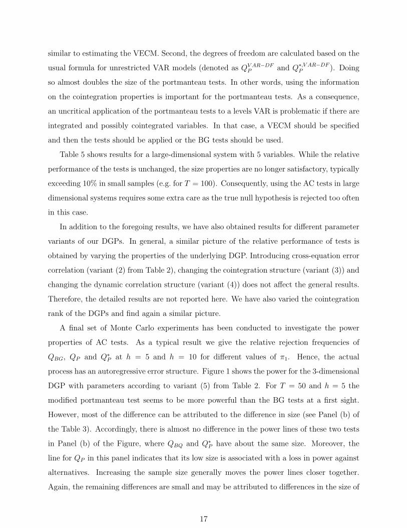
Table 5 shows results for a large-dimensional system with 5 variables. While the relative

performance of the tests is unchanged, the size properties are no longer satisfactory, typically

exceeding 10% in small samples (e.g. for T = 100). Consequently, using the AC tests in large

dimensional systems requires some extra care as the true null hypothesis is rejected too often

in this case.

In addition to the foregoing results, we have also obtained results for different parameter

variants of our DGPs. In general, a similar picture of the relative performance of tests is

obtained by varying the properties of the underlying DGP. Introducing cross-equation error

correlation (variant (2) from Table 2), changing the cointegration structure (variant (3)) and

changing the dynamic correlation structure (variant (4)) does not affect the general results.

Therefore, the detailed results are not reported here. We have also varied the cointegration

rank of the DGPs and find again a similar picture.

A final set of Monte Carlo experiments has been conducted to investigate the power

properties of AC tests. As a typical result we give the relative rejection frequencies of

QBG, QP and Q∗P at h = 5 and h = 10 for different values of π1. Hence, the actual

process has an autoregressive error structure. Figure 1 shows the power for the 3-dimensional

DGP with parameters according to variant (5) from Table 2. For T = 50 and h = 5 the

modified portmanteau test seems to be more powerful than the BG tests at a first sight.

However, most of the difference can be attributed to the difference in size (see Panel (b) of

the Table 3). Accordingly, there is almost no difference in the power lines of these two tests

in Panel (b) of the Figure, where QBQ and Q∗P have about the same size. Moreover, the

line for QP in this panel indicates that its low size is associated with a loss in power against

alternatives. Increasing the sample size generally moves the power lines closer together.

Again, the remaining differences are small and may be attributed to differences in the size of

17

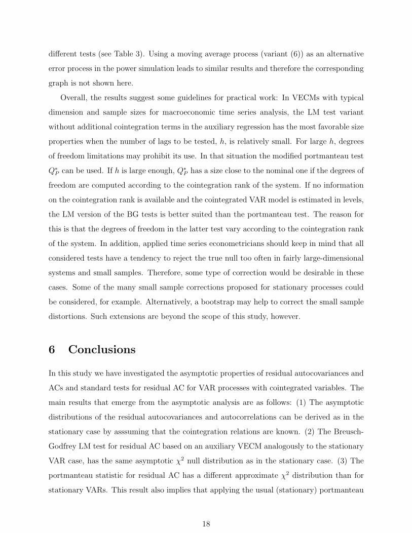
different tests (see Table 3). Using a moving average process (variant (6)) as an alternative

error process in the power simulation leads to similar results and therefore the corresponding

graph is not shown here.

Overall, the results suggest some guidelines for practical work: In VECMs with typical

dimension and sample sizes for macroeconomic time series analysis, the LM test variant

without additional cointegration terms in the auxiliary regression has the most favorable size

properties when the number of lags to be tested, h, is relatively small. For large h, degrees

of freedom limitations may prohibit its use. In that situation the modified portmanteau test

Q∗P can be used. If h is large enough, Q∗

P has a size close to the nominal one if the degrees of

freedom are computed according to the cointegration rank of the system. If no information

on the cointegration rank is available and the cointegrated VAR model is estimated in levels,

the LM version of the BG tests is better suited than the portmanteau test. The reason for

this is that the degrees of freedom in the latter test vary according to the cointegration rank

of the system. In addition, applied time series econometricians should keep in mind that all

considered tests have a tendency to reject the true null too often in fairly large-dimensional

systems and small samples. Therefore, some type of correction would be desirable in these

cases. Some of the many small sample corrections proposed for stationary processes could

be considered, for example. Alternatively, a bootstrap may help to correct the small sample

distortions. Such extensions are beyond the scope of this study, however.

6 Conclusions

In this study we have investigated the asymptotic properties of residual autocovariances and

ACs and standard tests for residual AC for VAR processes with cointegrated variables. The

main results that emerge from the asymptotic analysis are as follows: (1) The asymptotic

distributions of the residual autocovariances and autocorrelations can be derived as in the

stationary case by asssuming that the cointegration relations are known. (2) The Breusch-

Godfrey LM test for residual AC based on an auxiliary VECM analogously to the stationary

VAR case, has the same asymptotic χ2 null distribution as in the stationary case. (3) The

portmanteau statistic for residual AC has a different approximate χ2 distribution than for

stationary VARs. This result also implies that applying the usual (stationary) portmanteau

18

test for checking the residuals of a VAR model with integrated and cointegrated variables

has no sound theoretical basis.

We have also performed a small Monte Carlo study to check the finite sample perfor-

mance of the tests and found generally similar results as in earlier studies for stationary

processes. For relatively small systems and moderately large samples, the Breusch-Godfrey

QBG statistic can be recommended if only low order AC is tested. In contrast, the modified

portmanteau test Q∗P performs reasonably well if higher order AC is to be tested. For the

performance of the latter test it is important, however, that the cointegration rank of the

system is taken into account when the degrees of freedom for the approximate distribution

are determined. The test tends to reject far too often if it is applied to VARs in levels of

cointegrated variables without such adjustments. Also for higher dimensional systems, the

asymptotic distribution is generally a poor guide for small sample inference based on these

tests. Thus, one may consider small sample adjustments or perhaps bootstrap procedures

to correct for the size distortions in these cases.

Our results suggest that some commercial software for VAR and VECM analysis should

be modified. In particular, the p-values for the portmanteau tests reported by EViews are

apparently based on an incorrect approximate distribution when VARs with cointegrated

variables in levels or VECMs are considered. Moreover, asymptotic p-values could be pro-

vided by PcGive for tests of residual AC for VECMs based on our theoretical results. In

contrast, proper tests for residual AC of VECMs are available in JMulTi (Lutkepohl &

Kratzig (2004)).

Appendix. Proofs

In this Appendix the notation from the previous sections is used.

A.1 Proof of Lemma 1

As discussed after Proposition 1, we can use model (3.4). Hence,

ut = ∆xt − (X ′t ⊗ IK)φ− α(β∗ − β∗)′x∗t−1 − ν(0), t = 1, . . . , T, (A.1)

19

where φ = vec[α : Γ1 : · · · : Γp−1], β∗′= [β′ : τ (0)], β∗

′= [β′ : τ (0)] and x∗t−1 = [x′t−1 : −(t−1)]′.

Denoting the LS estimator of φ from the model

∆xt = (X ′t ⊗ IK)φ + ut (A.2)

by φ, we can express ut in (A.1) as

ut = ∆xt − (X ′t ⊗ IK)φ + wt = ut + wt, (A.3)

where wt = (X ′t ⊗ IK)(φ− φ)− α(β∗ − β∗)′x∗t−1 − ν(0). Thus,

Cj − Cj = T−1

T∑t=j+1

utw′t−j + T−1

T∑t=j+1

wtu′t−j + T−1

T∑t=j+1

wtw′t−j, (A.4)

and it suffices to show that each of the three terms on the right-hand side (r.h.s.) is of order

Op(T−1). To this end we shall first demonstrate that

φ− φ = Op(T−1). (A.5)

Define X∗t = [(β∗

′x∗t−1)

′, ∆x′t−1, . . . , ∆x′t−p+1]′. Then φ and ν(0) can be obtained by LS

estimation from the regression model

∆xt = (X∗′t ⊗ IK)φ + ν(0) + u∗t , (A.6)

where u∗t = ut−α(β∗−β∗)′x∗t−1. Using (3.5), the fact that τ (0) = 0 and well-known properties

of stationary and I(1) processes (see Johansen (1995, Appendix B.7)), it is straightforward

to check that the sample means of X∗t , u∗t and ut are of order Op(T

−1/2). From this it further

follows, using standard LS formulas, that

φ = φ +

(T∑

t=1

X∗t X∗′

t

)−1

⊗ IK

T∑t=1

(X∗t ⊗ IK)u∗t + Op(T

−1). (A.7)

Defining X∗t = [(β∗

′x∗t−1)

′, ∆x′t−1, . . . , ∆x′t−p+1]′, we get X∗

t − X∗t = [((β∗ − β∗)′x∗t−1)

′ : 0]′.

Hence, it follows from standard limit results for stationary and I(1) processes that

T−1

T∑t=1

(X∗t ⊗ IK)u∗t = T−1

T∑t=1

(X∗t ⊗ IK)ut + Op(T

−1)

and

T−1

T∑t=1

X∗t X∗′

t = T−1

T∑t=1

X∗t X∗′

t + Op(T−1).

20

Using these results and

φ = φ +

(T∑

t=1

XtX′t

)−1

⊗ IK

T∑t=1

(Xt ⊗ IK)ut (A.8)

together with (A.7), it is finally straightforward to obtain (A.5).

Now consider the first term on the r.h.s. of (A.4). By the definition of wt,

T−1

T∑t=j+1

utw′t−j = T−1

T∑t=j+1

ut(φ−φ)′(Xt⊗IK)−T−1

T∑t=j+1

utx∗′t (β∗−β∗)α′−T−1

T∑t=j+1

utν(0)′.

Because ut is the LS residual from a standard stationary regression model, limit results for

stationary and I(1) processes already used along with (3.5) and (A.5) show that the first two

terms on the r.h.s. are of order Op(T−1). That the same is true for the last term follows by

observing that the sample mean of ut is of order Op(T−1/2) and ν(0) = Op(T

−1/2) because

ν(0) = 0. Thus, the desired result has been established for the first term on the r.h.s. of

(A.4) and similar arguments clearly apply for the second term. The third term involves no

new features either, so details are omitted.

A.2 Proof of Proposition 1

According to Lemma 1, it suffices to show the proposition for the Cj. We therefore consider

the regression model (A.2) and the LS estimator φ. Defining Ut = [u′t−1, . . . , u′t−h]

′ gives

c = vec([C1, . . . , Ch]) = T−1

T∑t=1

(Ut ⊗ IK)ut,

where ut = 0 for t ≤ 0. Let c be the counterpart of c obtained by replacing ut by ut. Because

Xt is stationary and E(Xtu′t+j) = 0, j ≥ 0, it is straightforward to check that

c = c + T−1

T∑t=1

(Ut ⊗ IK)(ut − ut) + Op(T−1)

= c− T−1

T∑t=1

(UtX′t ⊗ IK)(φ− φ) + Op(T

−1)

(cf. Ahn (1988)). Denote MUX = T−1∑T

t=1 UtX′t = M ′

XU and define MUU and MXX

analogously. From the preceding representation of c and (A.8) we then find that

T 1/2c = [IhK2 : −(MUXM−1XX ⊗ IK)]T−1/2

T∑t=1

Ut ⊗ IK

Xt ⊗ IK

ut + Op(T

−1/2).

21

Proposition 1 follows from this result, plim T−1∑T

t=1 utu′t = Ω and

1√T

T∑t=1

Ut ⊗ IK

Xt ⊗ IK

ut

d→ N(0, Σ), (A.9)

where

Σ =

ΣUU ΣUX

ΣXU ΣXX

⊗ Ω

with ΣUU = Ih ⊗ Ω. The limit result in (A.9) follows from a standard martingale central

limit theorem using (2.3) (see Johansen (1995, Appendix B.7)).

References

Ahn, S. K. (1988). Distribution for residual autocovariances in multivariate autoregressive

models with structured parameterization, Biometrika 75: 590–593.

Doornik, J. A. (1996). Testing vector error autocorrelation and heteroscedasticity, unpub-

lished paper, Nuffield College.

Edgerton, D. & Shukur, G. (1999). Testing autocorrelation in a system perspective, Econo-

metric Reviews 18: 343–386.

Hosking, J. R. M. (1980). The multivariate portmanteau statistic, Journal of the American

Statistical Association 75: 602–608.

Hosking, J. R. M. (1981a). Equivalent forms of the multivariate portmanteau statistic,

Journal of the Royal Statistical Society B43: 261–262.

Hosking, J. R. M. (1981b). Lagrange-multiplier tests of multivariate time series models,

Journal of the Royal Statistical Society B43: 219–230.

Johansen, S. (1991). Estimation and hypothesis testing of cointegration vectors in Gaussian

vector autoregressive models, Econometrica 59: 1551–1581.

Johansen, S. (1995). Likelihood-based Inference in Cointegrated Vector Autoregressive Models,

Oxford University Press, Oxford.

22

Li, W. K. & McLeod, A. I. (1981). Distribution of the residual autocorrelations in multivari-

ate ARMA time series models, Journal of the Royal Statistical Society B43: 231–239.

Lutkepohl, H. (1991). Introduction to Multiple Time Series Analysis, Springer Verlag, Berlin.

Lutkepohl, H. & Kratzig, M. (eds) (2004). Applied Time Series Econometrics, Cambridge

University Press, Cambridge.

Mizon, G. E. & Hendry, D. F. (1980). An empirical application and Monte Carlo analysis

of tests of dynamic specification, Review of Economic Studies 47: 21–45.

Reinsel, G. C. & Ahn, S. K. (1992). Vector autoregressive models with unit roots and

reduced rank structure: Estimation, likelihood ratio test, and forecasting, Journal of

Time Series Analysis 13: 353–375.

Saikkonen, P. (2001a). Consistent estimation in cointegrated vector autoregressive models

with nonlinear time trends in cointegrating relations, Econometric Theory 17: 296–326.

Saikkonen, P. (2001b). Statistical inference in cointegrated vector autoregressive models

with nonlinear time trends in cointegrating relations, Econometric Theory 17: 327–356.

Saikkonen, P. (2003). Stability results for nonlinear error correction models, Technical report,

University of Helsinki.

23

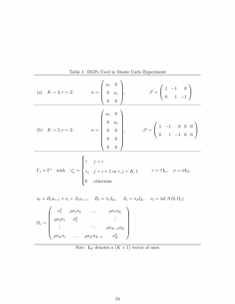
Table 1: DGPs Used in Monte Carlo Experiment

(a) K = 3, r = 2: α =

a1 0

0 a1

0 0

, β′ =

1 −1 0

0 1 −1

(b) K = 5, r = 2: α =

a1 0

0 a1

0 0

0 0

0 0

, β′ =

1 −1 0 0 0

0 1 −1 0 0

Γ1 = Γ∗ with γ∗ij =

γ j = i

γ1 j = i + 1 or i, j = K, 1

0 otherwise

τ = τ1r, ν = ν1K

ut = B1ut−1 + et + A1et−1, B1 = π1IK , A1 = π2IK , et ∼ iid N(0, Ωe)

Ωe =

σ21 ρσ1σ2 . . . ρσ1σK

ρσ2σ1 σ22

......

. . . ρσK−1σK

ρσKσ1 . . . ρσKσK−1 σ2K

Note: 1K denotes a (K × 1) vector of ones.

24

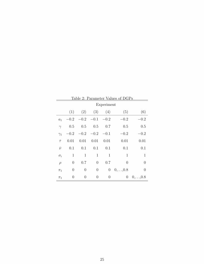
Table 2: Parameter Values of DGPs

Experiment

(1) (2) (3) (4) (5) (6)

a1 −0.2 −0.2 −0.1 −0.2 −0.2 −0.2

γ 0.5 0.5 0.5 0.7 0.5 0.5

γ1 −0.2 −0.2 −0.2 −0.1 −0.2 −0.2

τ 0.01 0.01 0.01 0.01 0.01 0.01

ν 0.1 0.1 0.1 0.1 0.1 0.1

σi 1 1 1 1 1 1

ρ 0 0.7 0 0.7 0 0

π1 0 0 0 0 0,. . .,0.8 0

π1 0 0 0 0 0 0,. . .,0.8

25

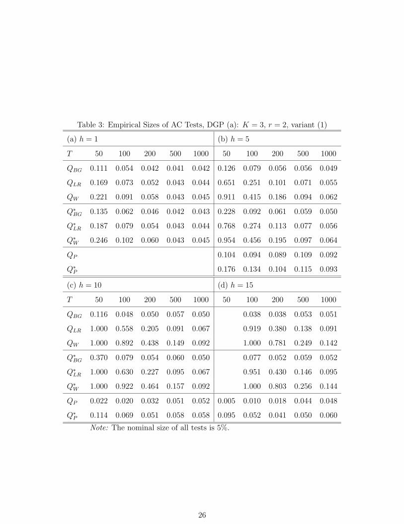
Table 3: Empirical Sizes of AC Tests, DGP (a): K = 3, r = 2, variant (1)

(a) h = 1 (b) h = 5

T 50 100 200 500 1000 50 100 200 500 1000

QBG 0.111 0.054 0.042 0.041 0.042 0.126 0.079 0.056 0.056 0.049

QLR 0.169 0.073 0.052 0.043 0.044 0.651 0.251 0.101 0.071 0.055

QW 0.221 0.091 0.058 0.043 0.045 0.911 0.415 0.186 0.094 0.062

Q∗BG 0.135 0.062 0.046 0.042 0.043 0.228 0.092 0.061 0.059 0.050

Q∗LR 0.187 0.079 0.054 0.043 0.044 0.768 0.274 0.113 0.077 0.056

Q∗W 0.246 0.102 0.060 0.043 0.045 0.954 0.456 0.195 0.097 0.064

QP 0.104 0.094 0.089 0.109 0.092

Q∗P 0.176 0.134 0.104 0.115 0.093

(c) h = 10 (d) h = 15

T 50 100 200 500 1000 50 100 200 500 1000

QBG 0.116 0.048 0.050 0.057 0.050 0.038 0.038 0.053 0.051

QLR 1.000 0.558 0.205 0.091 0.067 0.919 0.380 0.138 0.091

QW 1.000 0.892 0.438 0.149 0.092 1.000 0.781 0.249 0.142

Q∗BG 0.370 0.079 0.054 0.060 0.050 0.077 0.052 0.059 0.052

Q∗LR 1.000 0.630 0.227 0.095 0.067 0.951 0.430 0.146 0.095

Q∗W 1.000 0.922 0.464 0.157 0.092 1.000 0.803 0.256 0.144

QP 0.022 0.020 0.032 0.051 0.052 0.005 0.010 0.018 0.044 0.048

Q∗P 0.114 0.069 0.051 0.058 0.058 0.095 0.052 0.041 0.050 0.060

Note: The nominal size of all tests is 5%.

26

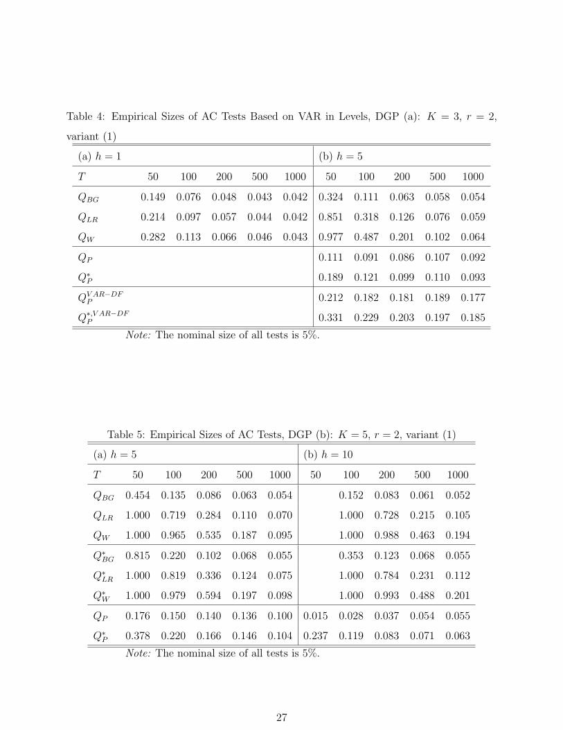
Table 4: Empirical Sizes of AC Tests Based on VAR in Levels, DGP (a): K = 3, r = 2,

variant (1)

(a) h = 1 (b) h = 5

T 50 100 200 500 1000 50 100 200 500 1000

QBG 0.149 0.076 0.048 0.043 0.042 0.324 0.111 0.063 0.058 0.054

QLR 0.214 0.097 0.057 0.044 0.042 0.851 0.318 0.126 0.076 0.059

QW 0.282 0.113 0.066 0.046 0.043 0.977 0.487 0.201 0.102 0.064

QP 0.111 0.091 0.086 0.107 0.092

Q∗P 0.189 0.121 0.099 0.110 0.093

QV AR−DFP 0.212 0.182 0.181 0.189 0.177

Q∗,V AR−DFP 0.331 0.229 0.203 0.197 0.185

Note: The nominal size of all tests is 5%.

Table 5: Empirical Sizes of AC Tests, DGP (b): K = 5, r = 2, variant (1)

(a) h = 5 (b) h = 10

T 50 100 200 500 1000 50 100 200 500 1000

QBG 0.454 0.135 0.086 0.063 0.054 0.152 0.083 0.061 0.052

QLR 1.000 0.719 0.284 0.110 0.070 1.000 0.728 0.215 0.105

QW 1.000 0.965 0.535 0.187 0.095 1.000 0.988 0.463 0.194

Q∗BG 0.815 0.220 0.102 0.068 0.055 0.353 0.123 0.068 0.055

Q∗LR 1.000 0.819 0.336 0.124 0.075 1.000 0.784 0.231 0.112

Q∗W 1.000 0.979 0.594 0.197 0.098 1.000 0.993 0.488 0.201

QP 0.176 0.150 0.140 0.136 0.100 0.015 0.028 0.037 0.054 0.055

Q∗P 0.378 0.220 0.166 0.146 0.104 0.237 0.119 0.083 0.071 0.063

Note: The nominal size of all tests is 5%.

27

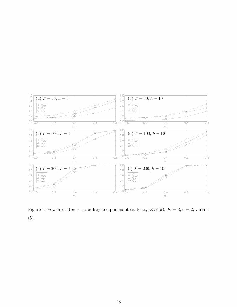
(a) T = 50, h = 5

(c) T = 100, h = 5

(e) T = 200, h = 5

(b) T = 50, h = 10

(d) T = 100, h = 10

(f) T = 200, h = 10

Figure 1: Powers of Breusch-Godfrey and portmanteau tests, DGP(a): K = 3, r = 2, variant

(5).

28