universit`a degli studi di torino - diunitophd/documents/tesi/xx/corderophdthesis.pdf ·...
TRANSCRIPT

Universita degli Studi di Torino
Dipartimento di InformaticaC.so Svizzera 185, 10149 Torino, Italy
DOTTORATO DI RICERCA IN INFORMATICA
Ciclo XX
Ph. D. thesis
Graphical models for the prediction of transcriptionfactor binding sites
Francesca Cordero
ADVISOR:
Prof. Marco BottaCO-ADVISOR:
Prof. Gary D. StormoTUTOR:
Prof. Giuliana Franceschinis
Ph. D. COORDINATOR:
Prof. Pietro Torasso

2

Acknowledgements
I would like to thanks to Professor Marco Botta for his help and continuous
encouragements in during the years of my Ph.D.
Professor Gary Stormo, for give me the opportunity to research in his
lab and for his support and more scientific suggestions.
Professor Giuliana Franceschinis and Raffaele Calogero for their com-
ments and careful reading.
All the great scientists and great colleagues I had the opportunity to
meet during this years at University of Turin and at WashU, from them
I have learned more. I am particularly grateful to Roberto Esposito and
Ryan Christensen.
I also would like thanks to my family for having stayed with me also this
time, as in all challenges of my life.
A very special thanks to Marco, for all scientific support, always being
an endless source of love, comfort and motivation. I dedicate this thesis to
him.

4

Contents
1 Introduction 3
2 Biological Background 7
2.1 From DNA to Protein . . . . . . . . . . . . . . . . . . . . . 7
2.2 DNA . . . . . . . . . . . . . . . . . . . . . . . . . . . . . . . 9
2.2.1 Nucleotides . . . . . . . . . . . . . . . . . . . . . . . 9
2.2.2 Structure and main features of DNA . . . . . . . . . 12
2.3 Genes . . . . . . . . . . . . . . . . . . . . . . . . . . . . . . 13
2.3.1 Regulatory Region . . . . . . . . . . . . . . . . . . . 15
2.4 Proteins . . . . . . . . . . . . . . . . . . . . . . . . . . . . . 17
2.4.1 Amino acids and protein structure . . . . . . . . . . 18
2.4.2 Protein organization . . . . . . . . . . . . . . . . . . 19
2.5 Structural Motifs of Gene Regulatory Proteins . . . . . . . . 22
2.5.1 The Helix-Turn-Helix Motif . . . . . . . . . . . . . . 23
2.5.2 The Zinc Finger Motif . . . . . . . . . . . . . . . . . 23
2.5.3 The β sheets Motif . . . . . . . . . . . . . . . . . . . 24
2.5.4 The Leucine Zipper Motif . . . . . . . . . . . . . . . 25
2.6 Crystal structure . . . . . . . . . . . . . . . . . . . . . . . . 25
3 State of the Art 27
3.1 DNA binding sites: representation . . . . . . . . . . . . . . . 27
3.2 DNA binding sites: identification . . . . . . . . . . . . . . . 31
3.2.1 Complete ab initio methodologies . . . . . . . . . . . 33
3.2.2 Partial ab initio methodologies . . . . . . . . . . . . 35
3.2.3 Matrix-based methodologies . . . . . . . . . . . . . . 39

CONTENTS ii
4 Graphical Models 43
4.1 Graph . . . . . . . . . . . . . . . . . . . . . . . . . . . . . . 45
4.2 Conditional Independence . . . . . . . . . . . . . . . . . . . 46
4.3 Markov Random Fields . . . . . . . . . . . . . . . . . . . . . 47
4.3.1 Conditional Independencies in Markov Random Fields 51
4.3.2 Example . . . . . . . . . . . . . . . . . . . . . . . . . 52
4.4 Bayesian Networks . . . . . . . . . . . . . . . . . . . . . . . 54
4.4.1 Conditional Independencies in Bayesian Networks . . 55
4.4.2 Example . . . . . . . . . . . . . . . . . . . . . . . . . 58
4.5 Learning . . . . . . . . . . . . . . . . . . . . . . . . . . . . . 58
4.6 Inference . . . . . . . . . . . . . . . . . . . . . . . . . . . . . 60
4.6.1 Gibbs Sampling . . . . . . . . . . . . . . . . . . . . . 61
4.6.2 Junction Tree . . . . . . . . . . . . . . . . . . . . . . 63
5 Representation of the crystal structure with graphical mod-
els 65
5.1 Links identification . . . . . . . . . . . . . . . . . . . . . . . 69
5.2 Graphical model construction . . . . . . . . . . . . . . . . . 73
5.3 Inference . . . . . . . . . . . . . . . . . . . . . . . . . . . . . 82
6 Results 84
6.1 Extraction of Crystal structures . . . . . . . . . . . . . . . . 87
6.2 Links identifications in Cys2His2 family . . . . . . . . . . . . 87
6.3 Data sets . . . . . . . . . . . . . . . . . . . . . . . . . . . . 92
6.4 Experimental Results . . . . . . . . . . . . . . . . . . . . . . 94
7 Discussion and future works 102

Abstract
An important challenge in molecular biology is to understand the mech-
anisms that regulate the expression of genes. A main step in this challenge
is the ability to identify regulatory elements in DNA, known as the Tran-
scription Factors Binding Sites (TFBS) or cis-regulatory. Moreover, the
genome research are interested to decipher the cis-regulatory code that gov-
erns complex transcriptional regulation. This apparently simple problem is
complicated by the fact that most TFBS are short, and they are character-
ized by sequence degeneration without loss of their function, which results
in a great variability in the binding sites for a single factor.
The discovery of motifs in sequences is an important topic of compu-
tational biology. In the last years has been develop many algorithms that
search in a different ways a list of features of TFBS allowing the discrimi-
nation between non-coding and coding sequence. The discrimination power
of this algorithms can be improved using acquired biological knowledge.
In many cases motifs discovery algorithms model DNA-protein inter-
actions using a set of Positional Weight Matrices (PWM) obtained from
TRANSFAC database as the input data. This search approach results in
a large number of hits characterized by many false positives. The limited
efficacy of these algorithms is due both to the limited amount of data used
to build a PWM, which is therefore a weak representation of the TFBS, and
to the assumption of independence among the positions in the motif, which
is an oversemplification.
In this thesis we have developed a method that infers the sequence speci-
ficity of a TF from x-ray co-crystal structure of DNA-protein interaction.
In our work we expand the probabilistic representation of DNA-protein
interaction using Markov Random Field and Bayesian Network built con-
sidering crystal data. In this way we want to model a structural (not only
textual) vision of DNA-protein interactions. contribute One of the major
contribute in this thesis is the mapping in every graphical model, of the
set of DNA-protein links that characterize a class of transcription factors.
CONTENTS 2
The results of the inference algorithm give a list of TFBSs ranked by a
probability value.
The crystal structure helps highlight the amino acids interacting with
specific positions of the DNA Binding Domain (DBD). If an amino acid
changes we know which positions in the DBD is changed and we can in-
fer which nucleotide interaction should also be changed. In this way we
can predict the binding motifs for new proteins not characterized from the
structural point of view.

Chapter 1
Introduction
An important challenge in molecular biology is the understanding of gene
expression regulation. Gene expression regulation is controlled by a com-
plex network of interactions involving DNA cis-regulatory elements, also
known as Transcriptions Factor Binding Sites (TFBS), and trans regulatory
polypeptides, transcription factors (TF). The binding of the TF to specific
sites on DNA is a central feature of transcriptional regulation. In general,
the motif that is recognized by DNA binding proteins is not a unique se-
quence. As a matter of fact recognition sites are a set of similar sequences
that are somewhat complementary in structure to their corresponding TFs
within a certain degree of variability.
Currently, genome-wide detection of DNA motif discovery algorithms
can be divided into three main classes: complete ab initio methodologies,
partial ab initio methodologies and matrix-based methodologies.
Since TFBS recognition is due to the chemical-physical interactions be-
tween amino acids in the DNA binding site of TF and the bases of TFBS, TF
binding site profiles should be predictable starting from protein-DNA com-
plex structures. Therefore, protein-DNA interaction roles could be grasped
from structural studies. TF binding sites could be predicted on the basis
of amino acids identities at the protein-DNA interface, resulting in simple
degenerated codes in which amino acid and base-pair combinations are cat-
egorised as either permissible or not. Although very intriguing, these codes
do not allow the prediction of affinities for different sequence combinations.
The most popular way of modeling binding sites assumes that each base

CHAPTER 1. INTRODUCTION 4
in the site occurs independently of the others. Methods based on this in-
dependence assumption between positions are relatively simple and based
on the definition of a limited set of parameters. These methods are widely
used and often producing acceptable models for binding site predictions.
However, recent experimental evidences shown the importance of the incor-
poration in the model of dependence on specific positions.
In this thesis we have developed a method for modeling the interaction
occurring between DNA and proteins in order to predict TFBS given a
protein sequence. We expanded the probabilistic representation of DNA-
protein interactions using graphical models built from crystal data. The core
of our approach is the detection in the 3D structure of DNA-TF complex,
of protein sequences positions linked to TFBS nucleotides. Since in crystal
structure these direct interactions are known and we can determine which
amino acid in a protein family plays a critical role in the interaction with
DNA and which is its specific interaction position in TFBS. As a result, we
model a structural vision of DNA-protein interactions.
Probabilistic graphical models are suitable for this task for several rea-
sons. They provide a concise language for describing probability distribu-
tions over the observations. The computational procedures for reasoning on
graphical models are derived from basic principles of probability theory.
Between the possible probabilistic graphical models we choose Markov Ran-
dom Fields (MRF) and Bayasian Network (BN). MRF belongs to the class
of undirected models. They represent a joint distribution as a product of po-
tentials. Each potential captures the interactions among a set of variables
and specifies the likelihood of joint value assignments to these variables.
The joint probabilities are determined by the overall compatibility of each
assignment of values according to all potentials. In BN the joint distribu-
tion over a set of random variables is represented as a product of conditional
probabilities. The graphical representation is given by a direct graph.

CHAPTER 1. INTRODUCTION 5
We use graphical models to obtain a more realistic approach to determine
a good way to capture the variability of the interactions between nucleotides
and amino acids. The graphical models allow to infer the best binding motif
in a family of transcriptional factors. Every graphical model represents a set
of DNA-protein links extracted from each crystal structure of a specif family
of TF. The mapping from DNA-protein complex to a graphical models is
not simple and is a significant contribution in this work. We starting from
the extraction of crystal structures: here, the main idea is to find which
positions in a protein sequence link to which positions in a TFBS. In a
crystal structure these direct interactions are known and we can determine
which critical amino acids in this protein family interacts with the DNA
and its specific position in TFBS. In a model-based approach we exploit
extensive biological domain knowledge to build the model that best fits the
links that characterize the DNA-protein interaction. The crystal structure
helps to highlight the amino acids interacting with specific positions of the
DNA Binding Domain (DBD) in a specific family of transcription factors.
In order to implement the graphical model we map the interaction using
edges and the nucleotides and amino acids positions using vertices.
Our aim is to learn a different set of nucleotide and amino acids recogni-
tion preferences for each of the vertices in the model. Then we need a set of
frequencies for every possible configuration of values in each links position.
Then, we are able to use our model as a predictor: given the observations
for all or some AA vertices, we can infer on DNA sequences that the protein
links.
In reading the following one needs to take into account that the empirical
assessment of the present system, especially in comparison to other systems,
is a difficult task. As a consequence the output of our system is conceptually
different from the output of state-of-the-art systems implying that a direct
comparison cannot be performed. On the other side, the ideal input of our
system is not publicly available yet. In order to deal with this difficulty,
we contented ourselves with less than optimal input data (the mutagenesis
data sets). This allowed to perform the experiments, but allegedly hindered

CHAPTER 1. INTRODUCTION 6
the results. The data sets that we use are have been selected form a set
of papers where biological experiments like SELEX and phage display have
been performed and affinity results are reported.
The inference algorithms applied on graphical models, return a list of
TFBSs ranked by a probability value. Differently from existing approaches
to TFBS prediction, that implicitly account for the information about the
DNA binding domain in the transcription factor, the developed model ex-
plicitly represents and uses this information to condition the probability of
the binding site.
This view on DNA-protein interaction was never investigated until now,
and represents an innovative way of looking at TFBS prediction. Moreover,
existing approaches can only check if a DNA sequence is likely to be a bind-
ing site for a known transcription factor, while the approach we developed
is able to also predict which is the most likely sequence of nucleotides that
binds to a new protein sequence.
Part of the work has been carry on during my visiting period at Washing-
ton University Medical School in St. Louis, in the Department of Genetics,
Center for Genome Sciences under supervision of prof. Gary Stormo.
This thesis is organized as follows: Chapter 2 present basic biological
background introduction to the concepts used in the rest of the thesis. If
the reader is already familiar with this knowledge, he can directly start with
Chapter 3, where we review the state of the art related to the representation
and discovery TFBSs. In Chapter 4 we introduce concepts and definitions
concerning the two graphical models: Markov Random Fields and Bayesian
Networks.
Chapter 5 present our contributions, the strategy that we use in order
to map the interactions data on graphical models as it has been published
in [23].
The results obtained in the thesis are describe in Chapter 6.
Finally in chapter 7, the conclusions and the possible future develop-
ments are outlined.
Chapter 2
Biological Background
It is bewildering that what separates humans from bacteria is merely the
organization and assembly of the same basic bio-molecules. At the micro-
scopic level, complex and simple organisms alike are made up of the same
unit of life, the cell. A cell contains all the information and machinery
necessary for its growth, maintenance and replication. Within a cell, virtu-
ally all functional roles are fulfilled by proteins, the most versatile type of
macro-molecule. Various types of proteins fulfill an immense array of tasks.
DeoxyriboNucleic Acid (DNA) in turn carries the genetic information that
encodes the precise sequence of all proteins, the signals that control their
production, and all other inheritable traits. The purpose of this chapter
is to provide a introduction to molecular biology, passing among the gen-
eral proprieties of DNA, proteins and RiboNucleic Acid (RNA) and genes
structure and regulation.
All this chapter is based on the main works in this area: [11], [35].
2.1 From DNA to Protein
Only when the structure of DNA was discovered in the early 1950s did it
become clear how the hereditary information in cells is encoded in DNA’s
sequence of nucleotides. Fifty years later, genome sequences was completed
for many organisms, including humans, therefore the maximum amount of
information that is required to produce a complex organism had known.
Much has been learned about how the genetic instructions written in
CHAPTER 2. BIOLOGICAL BACKGROUND 8
an alphabet of just four ”letters” (the four different nucleotides in DNA)
direct the formation of a bacterium, a fruit fly, or a human. Nevertheless,
we still have a great deal to discover about how the information stored
in an organism’s genome produces even the simplest unicellular bacterium
with 500 genes, let alone how it directs the development of a human with
approximately 30,000 genes.
Much of the DNA-encoded information present in all genomes is used to
specify the sequence of amino acids for every protein the organism makes.
The amino acid sequence in turn dictates how each protein folds to give a
molecule with a distinctive shape and chemistry. When a particular protein
is made by the cell, the corresponding region of the genome must therefore
be accurately decoded. Additional information encoded in the DNA of the
genome specifies exactly when and in which cell types each gene is to be
expressed into protein. Since proteins are the main constituents of cells, the
decoding of the genome determines not only the size, shape, biochemical
properties, and behavior of cells, but also the distinctive features of each
species.
Small bits of coding DNA (DNA that codes for protein) are interspersed
with large blocks of seemingly meaningless DNA. Some sections of the
genome contain many genes and others lack genes altogether. Proteins that
work closely with one another in the cell often have their genes located on
different chromosomes1, and adjacent genes typically encode proteins that
have little to do with each other in the cell. Even with the aid of compu-
tational approaches, it is still difficult to locate definitively the beginning
and end of genes in the DNA sequences of complex genomes, much less to
predict when each gene is expressed.
The DNA in genomes does not direct protein synthesis itself, but instead
uses RNA as an intermediary molecule. Transcription is the synthesis of
RNA under the direction of DNA. DNA sequence is copied by an enzyme to
produce a complementary nucleotide RNA strand, called messenger RNA
1Chromosomes are organized structures of DNA and proteins that are found in cells.
A chromosome is a continuous piece of DNA, which contains many genes, regulatory ele-
ments and other nucleotide sequences. Chromosomes also contain DNA-bound proteins,
which serve to package the DNA and control its functions.
CHAPTER 2. BIOLOGICAL BACKGROUND 9
(mRNA), because it carries a genetic message from the DNA to the protein-
synthesizing machinery of the cell. It is these mRNA copies of segments of
the DNA that are used directly as templates to direct the synthesis of the
protein translation. The flow of genetic information in cells is therefore
DNA⇒ RNA⇒ Protein
All cells, from bacteria to humans, express their genetic information in this
way. This principle is called the central dogma of molecular biology.
Despite the universality of the central dogma, there are important vari-
ations in the way information flows from DNA to protein. Principal among
these is that RNA transcripts in eucaryotic cells are subject to a series of
processing steps in the nucleus, like RNA splicing, before they are permitted
to exit from the nucleus and be translated into proteins. These processing
steps can critically change the ”meaning” of an RNA molecule and are there-
fore crucial for understanding how eucaryotic cells read the genome. Like
proteins, many of these RNAs fold into precise three-dimensional structures
that have structural and catalytic roles in the cell.
However, the simplified representation of the central dogma does not
reflect the role of proteins in the synthesis of nucleic acids. Moreover, as
discussed below, proteins are largely responsible for regulating gene expres-
sion that characterizes various cell types.
2.2 DNA
The names of James Watson and Francis Crick are so closely linked with
DNA that it is easy to forget that, when they began their collaboration
in October 1951, the detailed structure of the DNA polymer was already
known. Their contribution was not to determine the structure of DNA per
se, but to show that in living cells two DNA chains are intertwined to form
the double helix.
2.2.1 Nucleotides
DNA and RNA are a linear, unbranched polymer in which the monomeric
subunits are chemically distinct nucleotides, also called bases, that can be
CHAPTER 2. BIOLOGICAL BACKGROUND 10
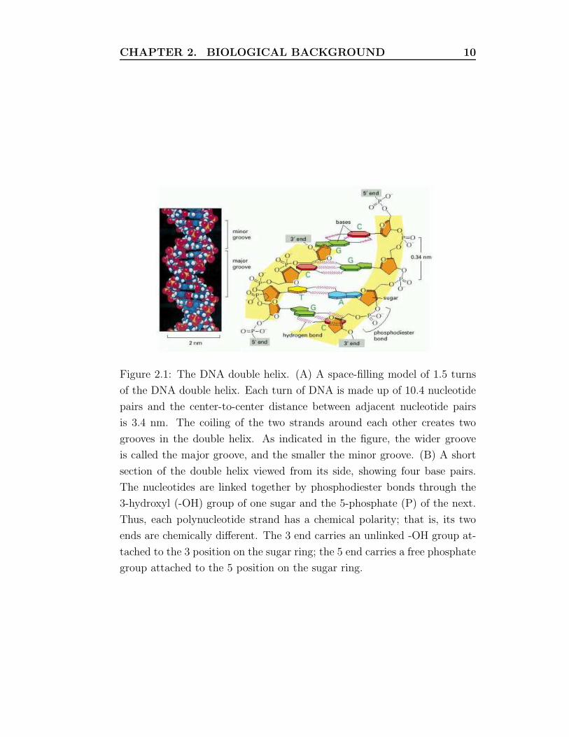
Figure 2.1: The DNA double helix. (A) A space-filling model of 1.5 turns
of the DNA double helix. Each turn of DNA is made up of 10.4 nucleotide
pairs and the center-to-center distance between adjacent nucleotide pairs
is 3.4 nm. The coiling of the two strands around each other creates two
grooves in the double helix. As indicated in the figure, the wider groove
is called the major groove, and the smaller the minor groove. (B) A short
section of the double helix viewed from its side, showing four base pairs.
The nucleotides are linked together by phosphodiester bonds through the
3-hydroxyl (-OH) group of one sugar and the 5-phosphate (P) of the next.
Thus, each polynucleotide strand has a chemical polarity; that is, its two
ends are chemically different. The 3 end carries an unlinked -OH group at-
tached to the 3 position on the sugar ring; the 5 end carries a free phosphate
group attached to the 5 position on the sugar ring.

CHAPTER 2. BIOLOGICAL BACKGROUND 11
Figure 2.2: The five different nitrogenous bases for the nucleotides guanine,
adenine, thymine, cytosine and uracil.
linked together in any order in chains hundreds, thousands or even millions
of units in length. Only four different bases are used in DNA molecules:
guanine, adenine, thymine and cytosine (G, A, T and C). Also the RNA
is composed by four nucleotides, three in common with DNA (guanine,
adenine and cytosine) and one specific in a RNA molecule uracil (U). Each
base is attached to a phosphate group and a sugar to form a nucleotide.
The sugar involved in the synthesis and structure of a nucleotide may be
either ribose or deoxyribose in RNA and DNA respectively. The only thing
that makes one nucleotide different from another is which nitrogenous base
it contains (see Figure 2.2).
The chemical linkage between adjacent nucleotides, commonly called
a phosphodiester bond, actually consists of two phosphoester bonds, that
connects the phosphate group of one nucleotide to the deoxyribose sugar
of the next. The linear sequence of nucleotides linked by phosphodiester
bonds constitutes the primary structure of nucleic acids.
CHAPTER 2. BIOLOGICAL BACKGROUND 12
2.2.2 Structure and main features of DNA
A single nucleic acid strand has a backbone composed of repeating pentose-
phosphate units from which the purine and pyrimidine bases extend as
side groups. A nucleic acid strand has an end-to-end chemical orientation:
the 5’ end and the 3’ end (see Figure 2.1). This directionality, plus the
fact that synthesis proceeds 5’ to 3’, has given rise to the convention that
polynucleotide sequences are written and read in the 5’→ 3’ direction (from
left to right); for example, the sequence AUG is assumed to be (5’)AUG(3’).
As we will see, the 5’→ 3’ directionality of a nucleic acid strand is an
important property of the molecule.
DNA consists of two associated polynucleotide strands that wind to-
gether to form a double helix. The two sugar phosphate backbones are on
the outside of the double helix, and the bases project into the interior. The
adjoining bases in each strand stack on top of one another in parallel planes.
The orientation of the two strands is antiparallel; that means that their 5’→
3’ directions are opposite. The strands are held in precise register by forma-
tion of base pairs between the two strands: A is paired with T through two
hydrogen bonds; G is paired with C through three hydrogen bonds. This
base-pair complementarity is a consequence of the size, shape, and chemi-
cal composition of the bases. The presence of thousands of such hydrogen
bonds in a DNA molecule contributes greatly to the stability of the double
helix. These associations between a larger purine and smaller pyrimidine
are often called Watson-Crick base pairs. Two polynucleotide strands in
which all the nucleotides form such base pair are said to be complementary.
For 20 years after the discovery of the DNA double helix in 1953, DNA
was thought to have the same monotonous structure, with exactly 36 of
helical twist between its adjacent nucleotide pairs (10 nucleotide pairs per
helical turn) and a uniform helix geometry. This view was based on struc-
tural studies of heterogeneous mixtures of DNA molecules and it changed
once the three-dimensional structures of short DNA molecules were deter-
mined using x-ray crystallography (section 2.6 for more details) and NMR
spectroscopy. Whereas the earlier studies provided a picture of an average,
idealized DNA molecule, the later studies showed that any given nucleotide
sequence had local irregularities, such as tilted nucleotide pairs or a heli-
CHAPTER 2. BIOLOGICAL BACKGROUND 13
cal twist angle larger or smaller than 36. These unique features can be
recognized by specific DNA-binding proteins.
Most of the DNA in eukaryotic cells is located in the nucleus, exten-
sively folded into the familiar structures we know as chromosomes. Each
chromosome contains a single linear DNA molecule associated with certain
proteins. The genome of an organism comprises its entire complement of
DNA.
2.3 Genes
Gene have different meanings for different point of views [57]: in classical
genetics, a gene was an abstract concept: a unit of inheritance that ferries
a characteristic from parent to child. As biochemistry came into its own,
those characteristics were associated with enzyme or proteins, one for each
gene. And with the advent of molecular biology, genes became real, physi-
cal things: sequences of DNA which when converted into strands of so-called
messenger RNA could be used as the basis for building their associated pro-
tein piece by piece. The great coiled DNA molecules of the chromosomes
were seen as long strings on which gene sequences sat like discrete beads.
Using the molecular biology definition most genes specify one or more
protein molecules, the ”expression” of these genes involving an RNA that is
used to direct synthesis of the protein. Other genes do not specify proteins,
the end-products of their expression being non-coding RNA, which plays
various roles in the cell.
The functions of about half of the 30.000/40.000 human genes are known
or can be inferred with a reasonable degree of certainty. The vast majority
code for proteins; less than 2500 specify the various types of non-coding
RNA. Almost a quarter of the protein-coding genes are involved in expres-
sion, replication and maintenance of the genome and another 20% specify
components of the signal transduction pathways that regulate genome ex-
pression and other cellular activities in response to signals received from
outside the cell.
Cell differentiation generally depends on changes in gene expression
rather than on any changes in the nucleotide sequence of the cell’s genome.

CHAPTER 2. BIOLOGICAL BACKGROUND 14
The different cell types in a multicellular organism differ dramatically in
both structure and function. Comparing a mammalian neuron with a lym-
phocyte, for example, the differences are so extreme that it is difficult to
imagine that the two cells contain the same genome. For this reason, cell dif-
ferentiation is often irreversible. The cell types in a multicellular organism
become different from one another because they synthesize and accumulate
different sets of RNA and protein molecules. They generally do this without
altering the sequence of their DNA but only by different regulation in gene
expression.
There are many steps in the pathway leading from DNA to protein, and
all of them can in principle be regulated. Thus a cell can control the proteins
it makes by:
• Controlling when and how often a given gene is transcribed, transcrip-
tional control.
• Controlling how the RNA transcript is spliced or otherwise processed,
RNA processing control.
• Selecting which completed mRNAs in the cell nucleus are exported to
the cytosol and determining where in the cytosol they are localized,
RNA transport and localization control.
• Selecting which mRNAs in the cytoplasm are translated by ribosomes,
translational control.
• Selectively destabilizing certain mRNA molecules in the cytoplasm
mRNA degradation control.
• Selectively activating, inactivating, degrading, or compartmentalizing
specific protein molecules after they have been made, protein activity
control.
The gene structure starts with the promoter region, which is followed
by a transcribed but non-coding region called 5’ untranslated region (5’
UTR). Then follows the coding region, this is usually not continuous, it is
composed of alternating stretches of exons (coding sequences) and introns
(non conding sequences). During transcription, both exons and introns are
CHAPTER 2. BIOLOGICAL BACKGROUND 15
transcribed onto the RNA, in their linear order. Thereafter, a process called
splicing takes place, in which, the intron sequences are excised and discarded
from the RNA sequence. The alternating sequence of exons and introns is
followed by another non-coding region called the 3’ UTR.
2.3.1 Regulatory Region
In the promoter region there are most of the regulatory region that control
the transcription of each gene. Some regulatory regions are simple and act
as switches that are thrown by a single signal. Many others are complex
and act as tiny microprocessors, responding to a variety of signals that they
interpret and integrate to switch the neighboring gene on or off. Whether
complex or simple, these switching devices contain two types of fundamental
components:
1. Short stretches of DNA of defined sequence, cis-factor.
2. Gene regulatory proteins, called Transcription Factors, TF that rec-
ognize and bind to them, trans-acting factor.
The fundamental units of gene regulation are the three types of spe-
cific DNA sequences that determine the level of expression under particular
physiological conditions [66]. Promoters, originally defined as elements that
determine the maximal potential level of gene expression, are recognized by
RNA polymerase II (the enzyme that makes an RNA copy of a DNA tem-
plate) and contain all the information necessary for accurate transcriptional
initiation. RNA polymerase II, which transcribes all protein-coding genes,
cannot initiate transcription on its own. It requires a set of proteins called
general transcription factors, which must be assembled at the promoter be-
fore transcription can begin. These proteinis help position the RNA poly-
merase correctly at the promoter. The term general refers to the fact that
these proteins assemble on all promoters transcribed by RNA polymerase
II; in this they differ from gene regulatory proteins, which act only at par-
ticular genes. This assembly process provides, in principle, multiple steps
at which the rate of transcription initiation can be speeded up or slowed
down in response to regulatory signals, and many TFs influence these steps.

CHAPTER 2. BIOLOGICAL BACKGROUND 16
The cells use transcriptional factor (activators and repressors) to regu-
late the expression of their genes but in a somewhat different way. Silencers
sequences are recognized by repressor proteins which inhibit transcription
that would otherwise occur from the promoters. Positive control elements,
enhancers, are recognized by activator proteins that stimulate transcription
from the promoter. The function of activators and repressors can be mod-
ulated by specific physiological conditions, thereby permitting regulated
expression of the cognate genes.
Efficient transcription generally requires the synergistic action of multi-
ple activator bound at distinct sites upstream (or downstream) for the pro-
moter. Thus, transcriptional activation is inherently combinatorial; each of
the large number of possible combinations is biologically distinct, and an
individual core promoter can be regulated with remarkable diversity and
precision.
Transcriptional factors must recognize specific nucleotide sequences em-
bedded within this structure. It was originally thought that these proteins
might require direct access to the hydrogen bonds between base pairs in the
interior of the double helix to distinguish between one DNA sequence and
another. The outside of the double helix is studded with DNA sequence
information that gene regulatory proteins can recognize without having to
open the double helix. The edge of each base pair is exposed at the surface of
the double helix, presenting a distinctive pattern of hydrogen bond donors,
hydrogen bond acceptors, and hydrophobic patches for proteins to recognize
in both the major and minor groove. But only in the major groove are the
patterns markedly different for each of the four base-pair arrangements. For
this reason, gene regulatory proteins generally bind to the major groove.
Although the patterns of hydrogen bond donor and acceptor groups are
the most important features recognized by gene regulatory proteins, they
are not the only ones: the nucleotide sequence also determines the overall
geometry of the double helix, creating distortions of the ”idealized” helix
that can also be recognized.
A specific nucleotide sequence can be detected as a pattern of structural
features on the surface of the DNA double helix. Particular nucleotide
sequences, each typically less than 20 nucleotide pairs in length, function

CHAPTER 2. BIOLOGICAL BACKGROUND 17
as fundamental components of genetic switches by serving as recognition
sites for the binding of specific gene regulatory proteins. Thousands of such
DNA sequences have been identified, each recognized by a different gene
regulatory protein (or by a set of related gene regulatory proteins).
Molecular recognition in biology generally relies on an exact fit between
the surfaces of two molecules, and the study of gene regulatory proteins
has provided some of the clearest examples of this principle. A gene reg-
ulatory protein recognizes a specific DNA sequence because the surface of
the protein is extensively complementary to the special surface features of
the double helix in that region. In most cases the protein makes a large
number of contacts with the DNA, involving hydrogen bonds, ionic bonds,
and hydrophobic interactions. Although each individual contact is weak,
the 20 or so contacts that are typically formed at the protein-DNA inter-
face add together to ensure that the interaction is both highly specific and
very strong. In fact, DNA-protein interactions include some of the tightest
and most specific molecular interactions known in biology.
2.4 Proteins
Proteins (also known as polypeptides), the working molecules of a cell, carry
out the program of activities encoded by genes. From a chemical point
of view, they are by far the most structurally complex and functionally
sophisticated molecules known. The structure and chemistry of each protein
has been developed and fine tuned over billions of years of evolutionary
history.
The proteins acquired specialized abilities and can be grouped into sev-
eral broad functional classes: structural proteins, which provide structural
rigidity to the cell; transport proteins, which control the flow of materials
across cellular membranes; regulatory proteins, which act as sensors and
switches to control protein activity and gene function; signaling proteins,
including cell surface receptors and other proteins that transmit external
signals to the cell interior; and motor proteins, which cause motion. Several
critical and complex cell processes synthesis of nucleic acids and proteins,
signal transduction, and photosynthesis are carried out by huge complexes

CHAPTER 2. BIOLOGICAL BACKGROUND 18
Figure 2.3: The amino acids. A) Amino acids possess common fea-
tures: 1)NH2 amino group, 2)central hydro-carbon group, 3) COOH (car-
boxyl)group,4) R group, specific to each amino acid. B) Both three-letter
and one-letter abbreviations are listed. The R group is possibly split in two
main groups based on the polarity of the side chain.
of protein, sometimes called molecular machines.
A protein molecule is made from a long chain of amino acids. Each
type of protein has a unique sequence of amino acids. Many thousands
of different proteins are known, each with its own particular amino acid
sequence.
2.4.1 Amino acids and protein structure
The 20 amino acids have similar chemical structure, varying only in the
chemical group attached in the R position. The constant region of each
amino acid is called the backbone, while the varying R group is called the
side chain. As DNA, the protein chain has directionality. One end of the
protein chain has free amino (NH2) group (its N-terminus), while the other
end of the chain terminates in a carboxylic acid (COOH) group (its C-
terminus),see Figure 2.3. The individual amino acids in the protein are
usually numbered starting at the amino terminus and proceeding toward
the carboxy terminus. The sequence of a protein chain is conventionally
written with its N-terminal amino acid on the left and its C-terminal amino
acid on the right.
Each amino acid is linked to the other in a head-to-tail way by a covalent
linkage, called peptide bond. As a consequence of the peptide linkage, the
backbone exhibits directionality because all the amino groups are located
CHAPTER 2. BIOLOGICAL BACKGROUND 19
on the same side of the Cα atoms. The primary structure of a protein is
simply the linear sequence of the amino acids residues that compose it. The
second level of protein structure consists of the various spatial arrangements
resulting from the folding of localized parts of a polypeptide chain. These
arrangements are referred to as secondary structures. A single protein may
exhibit multiple types of secondary structure depending on its sequence.
The three principal types of structures are alpha (α) helix, beta (β) sheet
and Turns. α helix forms when the carbonyl oxygen atom of each peptide
bond is hydrogen bonded to the amide hydrogen atom of the amino acid four
residues toward the C-terminus. beta (β) sheet consists of laterally packed
by hydrogen bonding between back bone adjacent of β strands (5-8 residues
nearly fully extended polypeptide segment). Turns are composed of three
or four residues and are located on the surface of a protein forming sharp
bends that redirect the polypeptide backbone back toward the interior. The
third structure refers to overall conformation of a polypeptide chain, that is,
the three-dimensional arrangement of all its amino acid residues stabilized
by hydrophobic interactions hydrogen bonds and peptide bonds.
To understand the structures and functions of proteins, it is necessary
to understand some of the distinctive properties of amino acids, which are
determined by their side chains. The side chains of different amino acids
vary in size, shape, charge, hydrophobicity, and reactivity. Amino acids can
be classified into several broad categories based primarily on their solubility
in water. Amino acids with polar side chains are hydrophilic and tend to be
on the surfaces of proteins; by interacting with water, they make proteins
soluble in aqueous solutions. In contrast, amino acids with nonpolar side
chains are hydrophobic; they avoid water and often aggregate to help form
the water insoluble cores of many proteins. The polarity of amino acid side
chains thus is responsible for shaping the final three dimensional structure
of proteins.
2.4.2 Protein organization
Studies of the conformation, function, and evolution of proteins have re-
vealed the central importance of a unit of organization. The organization of
large proteins into multiple domains illustrates the principle that complex

CHAPTER 2. BIOLOGICAL BACKGROUND 20
molecules are built from simpler components.
The term motif refers to a set of contiguous secondary structure elements
that either have a particular functional significance or define a portion of
an independently folded domain. An example is the helix-turn-helix mo-
tif found in many DNA-binding proteins, explained in section 2.5.1. This
simple structural motif will not exist as a stably folded domain if expressed
separately from the rest of its protein context, but when it can be detected
in a protein that is already thought to bind nucleic acids, it is a likely
candidate for the recognition element.
The tertiary structure is typically subdivided into distinct regions called
domains. From the structural point of view, a domain is a compactly
folded region of a protein. The protein domain consists of 100-150 residues
in various combinations of motifs. Often a domain is characterized by some
interesting structural feature: an unusual abundance of a particular amino
acid, sequences common to (conserved in) many proteins or a particular
secondary-structure motif. Domains are sometimes defined in functional
terms on the basis of observations that an activity of a protein is localized
to a small region along its length. For instance, a particular region of a
protein may be responsible for its catalytic activity or binding ability (e.g.,
a DNA-binding domain, a membrane-binding domain). In large proteins
a ”modular approach” to protein architecture is easily recognized. These
proteins are like a mosaic of different domains which can perform different
functions simultaneously.
In addition to primary, secondary and third levels of structural organi-
zation, proteins have a quater level, see Figure 2.4. A fourth level of struc-
tural organization, also called quaternary structure, describes the number
and relative positions of the subunits in multimeric proteins.
The links between the different levels of protein structure are more
clearly understood at the primary-to-secondary level. Because of the chem-
ical properties of their R groups, certain amino acids are more commonly
found in αhelices while others have a predisposition for βsheets. A seconda-
ry structure therefore forms around a group of amino acids that favor that
particular secondary structure and initiate its formation. It then extends
to include adjacent amino acids that either favor the structure or have no

CHAPTER 2. BIOLOGICAL BACKGROUND 21
Figure 2.4: Different levels of protein structure. (A) Primary structure.
(B) Secondary structure. The polypeptide shown in part a is drawn into an
α helix by hydrogen bonds. (C) Tertiary structure: the three-dimensional
structure of myoglobin. (D) Quaternary structure: the arrangement of two
α subunits and two β subunits to form the complete quaternary structure
of hemoglobin
.
CHAPTER 2. BIOLOGICAL BACKGROUND 22
strong disinclination towards it, and finally terminates when one or more
blocking amino acids, which cannot participate in that particular type of
structure, are reached. This process is repeated along the polypeptide until
each part of the chain has adopted its preferred secondary structure.
By identifying which amino acids are most frequently located in which
secondary structures, and by studying the structures taken up by small
polypeptides of known sequence, biochemists have been able to deduce rules
for this level of protein folding, and, to a certain extent, can predict which
secondary structures will be adopted by a polypeptide simply by examining
its primary sequence [7]. It is less easy to predict the outcomes of the next
two stages of protein folding, which result in the secondary structural units
becoming arranged into the tertiary structure, and tertiary units associat-
ing to form quaternary multi-subunit structures. The tertiary structures
of most proteins are made up of two or more structural domains, possibly
with little interaction between them; these domains are thought to fold in-
dependently of one another. The difficulty in identifying rules for predicting
tertiary and quaternary structures does not detract from the fact that these
higher levels of structure are determined by the amino acid sequence of the
polypeptide.
2.5 Structural Motifs of Gene Regulatory Pro-
teins
The DNA-binding domains of eucaryotic activator and repressor contain
a variety of structural motifs that bind specific DNA sequences. These
motifs generally use either helices or sheets to bind to the major groove
of DNA; this groove contains sufficient information to distinguish one DNA
sequence (Transcriptional Factor Binding Site, TFBS ) from any other. The
fit is so good that it has been suggested that the dimensions of the basic
structural units of nucleic acids and proteins evolved together to permit
these molecules to interlock. Here we introduce several common classes of
DNA-binding proteins.

CHAPTER 2. BIOLOGICAL BACKGROUND 23
2.5.1 The Helix-Turn-Helix Motif
The first DNA-binding protein motif to be recognized was the helix-turn-
helix (HTH), also called helix-loop-helix. It is constructed from two α helices
connected by a short extended chain of amino acids, which constitutes the
turn. The two helices are held at a fixed angle, primarily through interac-
tions between the two helices. The C-terminal helix is called the recognition
helix because it fits into the major groove of DNA; its amino acid side chains,
which differ from protein to protein, play an important part in recognizing
the specific DNA sequence to which the protein binds.
Outside the helix-turn-helix region, the structure of the various proteins
that contain this motif can vary enormously. Thus each protein presents its
HTH motif to the DNA in a unique way, a feature thought to enhance the
versatility of the HTH motif by increasing the number of DNA sequences
that the motif can be used to recognize. Moreover, in most of these proteins,
parts of the polypeptide chain outside the HTH domain also make important
contacts with the DNA, helping to fine-tune the interaction.
The group of helix-turn-helix proteins is a class of dimeric transcriptional
factor. Dimeric TF bind as symmetric dimers to DNA sequences that are
composed of two very similar half-sites, which are also arranged symmet-
rically. This arrangement allows each protein monomer to make a nearly
identical set of contacts and enormously increases the binding affinity.
2.5.2 The Zinc Finger Motif
Another important group of DNA-binding motifs adds one or more zinc
atoms as structural components. All such zinc-coordinated DNA-binding
motifs are called zinc fingers. Subsequent structural studies have shown that
they fall into several distinct structural groups. The first type was initially
discovered in the protein that activates the transcription of a eucaryotic
ribosomal RNA gene. It is a simple structure, consisting of an α helix and a
β sheet held together by the zinc. This type of zinc finger is often found in
a cluster with additional zinc fingers, arranged one after the other so that
the α helix of each can contact the major groove of the DNA, forming a
nearly continuous stretch of α helices along the groove. In this way, a strong

CHAPTER 2. BIOLOGICAL BACKGROUND 24
and specific DNA-protein interaction is built up through a repeating basic
structural unit. A particular advantage of this motif is that the strength and
specificity of the DNA-protein interaction can be adjusted during evolution
by changes in the number of zinc finger repeats.
The first most common DNA-binding motif is C2H2 zinc finger, this mo-
tif has two conserved cysteine (C) and two conserved histidine (H)residues,
whose side chains bind one Zn2+ ion. Many transcription factors contain
multiple C2H2 zinc fingers, which interact with successive groups of base
pairs, within the major groove, as the protein wraps around the DNA double
helix. A second type of zinc finger structure, the C4 zinc finger, is composed
by four conserved cysteines in contact with Zn2+ ion. A particular impor-
tant difference between the two is that C2H2 zinc-finger proteins generally
contain three or more repeating finger units and bind as monomers, whereas
C4 zinc finger proteins generally contain only two finger units and generally
bind to DNA as dimer, homodimer (composed of two identical motifs linked
together) or eterodimer (composed of two different motifs linked together).
2.5.3 The β sheets Motif
In the DNA-binding motifs discussed so far, α helices are the primary mech-
anism used to recognize specific DNA sequences. This group of gene reg-
ulatory proteins has evolved an entirely different recognition strategy. In
this case the information on the surface of the major groove is read by a
two-stranded β sheet, with side chains of amino acids extending from the
sheet toward the DNA. β sheet, consists of laterally packed β strands. Each
β strand is a short (from 5 to 8 residue), nearly fully extended polypeptide
chain. Hydrogen bonding between backbone atoms in adjacent β strands,
within either the same or different polypeptide chains, forms a β sheet. As
in the case of a recognition α helix, this β sheet motif can be used to rec-
ognize many different DNA sequences; the exact DNA sequence recognized
depends on the sequence of amino acids that make up the β sheet.
CHAPTER 2. BIOLOGICAL BACKGROUND 25
2.5.4 The Leucine Zipper Motif
The first transcription factors recognized in this class contained the hy-
drophobic amino acid leucine at every seventh position in the C-terminal
portion of their DNA-binding domains. These proteins bind to DNA as
dimers showed that they were required for dimerization. Consequently, the
name leucine zipper was coined to denote this structural motif.
Crystallographic analysis (see refCryStr) of complexes between DNA
and this type of domain has shown that the dimeric protein contains two
extended α helices that ”grip” the DNA molecule, much like a pair of scis-
sors, at two adjacent major grooves separated by about half a turn of the
double helix. The portions of the α helices contacting the DNA include basic
residues that interact with phosphates in the DNA backbone and additional
residues that interact with specific bases in the major groove.
Leucin-zipper proteins dimers via hydrophobic interactions between the
C-terminal regions of the α helices, forming a coiled-coil structure. This
structure is common in proteins containing amphipathic α helices in which
hydrophobic amino acid residues are regularly spaced alternately three or
four positions apart in the sequence. As a result of this characteristic spac-
ing, the hydrophobic side chains form a stripe down one side of the α helix.
These hydrophobic stripes make up the interacting surfaces between the α
helical monomers in a coiled-coil dimer.
The first transcription factors in this class to be analyzed contained
leucine residues at every seventh position in the dimerization region and
thus were named leucine-zipper proteins. However, additional DNA-binding
proteins containing other hydrophobic amino acids in these positions subse-
quently were identified. Like leucine-zipper proteins, they form dimers con-
taining a C-terminal coiled-coil dimerization region and N-terminal DNA-
binding domain.
2.6 Crystal structure
An increasing number of structural studies are aimed at identifying the
principles that govern protein-DNA recognition in gene regulation. This
work depends on the successful reconstruction of protein-DNA complex from

CHAPTER 2. BIOLOGICAL BACKGROUND 26
their purified components.
To figure out how a protein works, its three-dimensional structure must
be known. Determining a proteins conformation requires sophisticated
physical methods and complex analyses of the experimental data.
While even the most powerful microscopy techniques are insufficient to
determine the molecular coordinates of each atom in a protein, the discov-
ery of X-rays has led to the development of a powerful tool for analyzing
protein structure: x-ray crystallography. The first step on crystallographic
determination of a protein’s structure is to grow a crystal of the protein.
Just a sugar crystals are often grown by slow evaporation of a solution of
sugar and water, protein crystals are often grown by evaporation of a pure
protein solution. Protein crystals, however, are generally very small (0.3 to
1.5 mm in each dimension), and consist of as much as 70% water. Growing
protein crystal generally requires carefully controlled conditions and a great
deal of time; it sometimes take months or even years of experimentation
to find the appropriate crystallization condition for a single protein. Once
protein crystals are obtained, they are loaded into a capillary tube and ex-
posed to a beam of X-ray radiation, which is then diffracted by the protein
crystal. In early crystallography, the diffraction pattern was captured on
x-ray film. Modern crystallography equipment uses x-ray detectors that
transfer the diffraction pattern directly to a computer for analysis. Once
the diffraction data are obtained, a crystallographer uses a very complex
mix of reverse Fourier transformations, crystallographic software tools and
protein modelling skills to determine the three dimensional structure of the
protein.
Chapter 3
State of the Art
An important challenge in molecular biology is the understanding of gene
expression regulation. Gene expression regulation controlled by a com-
plex network of interactions involving DNA cis-regulatory elements, also
known as Transcriptions Factor Binding Sites (TFBS), and trans regula-
tory polypeptides, transcription factors (TF).
An important open question for the comprehension of a gene expression
regulation is the mapping of TFBS. The purpose of this chapter is to provide
a brief introduction to the main algorithms for the analysis and prediction
of DNA binding sites described in the literature. In section 3.1 we will
introduce the necessary background to understand these algorithms. In
section 3.2 we will present the algorithms in details.
3.1 DNA binding sites: representation
In the last 30 years a lot of date have been obtained about transcription
factor interactions with DNA sequences also due to the development of
more efficient sequencing methods which allowed the massive sequencing of
multiple genomes. Thanks to this, the total amount of genomic sequences
annually was increasing rapidly and highlight the need of dedicated algo-
rithms for identification of regulative sequences (i.e. TFBS). For instance,
TFBSs can be represented by strings based on 4-letter alphabet [A, C, G,
T], called base or nucleotide, so that all pattern matching algorithms can
be used to map them in DNA sequences.

CHAPTER 3. STATE OF THE ART 28
Figure 3.1: Representation of transcription-factor binding sites. (a) An
example of six sequences and the consensus sequence that can be derived
from them. The consensus simply gives the nucleotide that is found most
often in each position; the alternate (or degenerate) consensus sequence
gives the possible nucleotides in each position; R represents A or G; N
represents any nucleotide. (b) A position weight matrix for the -10 region of
E. coli promoters, as an example of a well-studied regulatory element. The
boxed elements correspond to the consensus sequence (TATAAT). The score
for each nucleotide at each position is derived from the observed frequency of
that nucleotide at the corresponding position in the input set of promoters.
The score for any particular site is the sum of the individual matrix values
for that site’s sequence; for example, the score for TATAAT is 85. Note that
the matrix values in (b) do not come from the example shown in (a) but
rather are derived from a much larger collection of -10 promoter regions [30].
CHAPTER 3. STATE OF THE ART 29
In order to capture the variability of TFBSs, it is necessary to use a
set of single character codes that represent all possible combinations of
nucleotides. The consensus sequence is a sequence that shows both con-
served and variable bases in transcription factors binding sites (an example
is shown in Figure 3.1). In consensus definition, after aligning some binding
sites (so that they match each other), if one position contains 70% adenine,
10% cytosine, 10% guanine and 10% thymine, the consensus for this posi-
tions is the most represented base ‘A’. TFBSs representation by consensus
sequence frequently results in a distorted pictures of binding sites [69]. A
problem arises when a position that is 100% ’A’ in the original set is treated
in the same way of another one which is represented by an ‘A’ only in 70%
of all the sequences. This reduces the efficacy of consensus sequence in the
detection of TFBSs. In this example, we will find mismatches for 30% of
the acceptable sequences.
An alternative to consensus sequences for representing a TFBS is given
by the Positional Weight Matrix (PWM). The PWM is a formalism to rep-
resents DNA motifs using on the statistical properties of a collection of TF-
BSs. The PWMs are able to capture, in quantitative way, the variability of
a collection of DNA sites, which is missed if DNA consensus sequences [16].
Therefore, PWM summarizes the statistical properties of a collection of
TFBS, where every position in the site corresponds to a column in PWM,
Figure 3.1(B).
The score for any particular site is given by the sum of the matrix values
for that site’s sequence. Any sequence that differs from the consensus will
have a lower score. PWMs represent a convenient way to account that some
positions are more highly conserved than others, and presumably are more
important for the activity of the site.
Since, PWMs are based on the observed sites on which they are built,
the sites sample size used to build PWM is an important issue affecting the
ability of a PWM to capture TFBS. This results in false negative calls on
the new sites that do not match well with the previous characterization [3].
Bussemaker at al. [37] give a new interpretation of the information en-
coded by PWM. In their view PWMs contain two kinds of knowledge:
the thermodynamics interactions between Transcription Factor (TF) (Sec-

CHAPTER 3. STATE OF THE ART 30
tion 2.3 for more details) and DNA, and evolutionary selection. The under-
lying assumptions are that natural selection gives rise to a certain level of
sequence specificity for each TF and sequences that give rise to the same
physically binding affinity are equally likely to be selected. In this view,
PWM should represent the properties of the DNA Binding Domain (DBD)
of a TF, instead of the properties for DNA motifs. Moreover, the additiv-
ity of the binding energy for each base pair is assumed. Provided that the
selected model assumptions are satisfied, the discrimination energy associ-
ated with the TF-DNA interaction at a given position in the binding site
is proportional to the logarithm of the ratio between the frequency in the
PWM and the background frequency for each nucleotide [31].
According with the additivity assumption each position contributes in-
dependently to the total binding energy, there is some matrix H(b, i) that
contains those binding energy contributions as its elements. Given any par-
ticular sequence Sα its total binding energy is since given by H(b, i) · Sα.
The measure of significance for one position in the PWM, compared with
the frequency in the genome, is commonly given by the Information Content
(IC) defined by [70]:
Ii = 2 +
T∑
b=A
fb,i log2 fb,i (3.1)
where i is the position in the site, b refers to each of the possible nucleotides,
and fb,i is the observed frequency of each base at ith position. The I values
are between 0, for positions that are 25% of each base, and 2 bits for posi-
tions completely conserved1. This formula provides a good approximation
only in genomes with a perfect balance distribution of frequency among
the four nucleotides (25% for each bases). Berg et al. [26] shows that the
logarithms of base frequencies should be proportional to the binding en-
ergy contribution of the bases. Equation 3.1 can be generalized accounting
genomic base probabilities:
1The information content is measured in bits. In the case of DNA sequences, this
measure ranges from 0 to 2 bits. A position in the motif at which all nucleotides occur
with equal probability has an information content of 0 bits, while a position at which
only a single nucleotide can occur has an information content of 2 bits.

CHAPTER 3. STATE OF THE ART 31
Iseq(i) =∑
b
fb,i log2
fb,i
pb
(3.2)
It is notable that IC corresponds to high variability in the site. [16].
A limitation of the weight matrix approach is given by the assumption
that the positions in site contribute additively to the total activity. More
complex models are possible in the framework of the matrix method but they
require some prior information about which positions are non-independent.
Currently, there are two comprehensive and annotated databases that
contain information on TFs binding site profiles: JASPAR [2] which con-
tains a smaller set that is non-redundant (each TF has only one profile),
and TRANSFAC [73] which contains multiple profile models for some TFs.
3.2 DNA binding sites: identification
The identification id TFBSs organization nearby gene transcription initia-
tion site, i.e. promoter analysis, represents a mandatory issue to define the
regulative networks of protein-DNA relations that control gene expression
in eukariotic cells.
TFBSs occurrences in a specific genome and their evolutionarily con-
servation among different species allow their computational retrieval. This
means that regulatory elements can be discovered by searching for over
represented motifs across promoters [33].
The interest in promoter analysis received a great improvement due to
the identification of co-regulated groups of gene, i.e. genes characterized by
similar expression profiles, by mean of high-throughput genome-wide tran-
scription analysis. A basic assumption is that these profiles reflect a similar
structure of the regions involved in transcription regulation. To understand
the common regulative structure of promoter regions of co-regulated genes,
a standard approach is the reduction of the complexity of the analysis.
Therefore as fist step, single common motifs are searched in co-regulated
gene promoter regions (Section 2.3 for more details) [72]
However, this apparently simple approach is complicated by the fact
that most TFBSs are short, and they can have some sequence degeneration
CHAPTER 3. STATE OF THE ART 32
without loss of function. There can be a great variability in the binding
sites for a single factor and the nature of the allowable variations is not well
understood [63]. Moreover it has been estimated that in human DNA about
3% of intergenic regions are regulatory elements [44]e.g. enanchers. This
means that several motifs are also found as random hits throughout the
genome so that a challenging problem to distinguish between false positive
sites and true positive binding sites arises. Hence motif searching can be
considered as a signal-to-noise problem.
For this reason most algorithms for identification of genomic regulatory
elements use orthogonal data.
For instance several algorithms include additional prior knowledge about
gene regulation: regulatory elements are not randomly distributed, but they
are clustered in transcription modules [27], and the presence of co-occurring
motifs can be used to identify putative regulatory modules.
Transcription modules are“self-consistent regulatory units”: a set of
genes are co-regulated, responding to different conditions that alter expres-
sion of all genes in the module. The modular structure discovered in the
genome-wide gene expression data may be due to the co-regulations of mul-
tiple genes by the same modulators that are activated or suppressed under
different conditions. Transcription modules are conceptually distinct from
cluster of co-expressed genes, because transcription modules represent self-
consistent subset of both genes and conditions such that all conditions of a
module affect all genes in the module, and different modules can overlap,
sharing some genes and/or conditions. Specific arrangements of TFBS into
transcription modules are necessary to achieve proper biological function.
Promoter analysis in many organisms has confirmed the modular architec-
ture of promoter sequences, and algorithms devoted to the identifications of
transcription modules can be based on a given set of DNA motifs or by“de
novo” methodologies.
Another type of orthogonal data are functional sequences that are pref-
erentially conserved over the course of evolution by selective pressure: this is
another characteristic, with the over representation, that Cora et al. [15] ap-
plied to determine transcription factor binding sites in the human genome.
The hypothesis that many orthologous genes expressed similarly in a tissue-
CHAPTER 3. STATE OF THE ART 33
specific manner in human and mouse, are likely to be co-regulated by or-
thologous transcriptional factors is the basis of the cis-regulatory regions
search [10].
It is worth noting that the analysis of non-coding regions in eukaryotic
genome (Section2.2 for more details) in order to identify regulatory elements
is a difficult problem not well solved yet [45].
The DNA motif discovery algorithms that have been developed can be di-
vided into three main classes [22]:
• Complete ab initio methodologies: parameter-free algorithms for
de novo identification of potential TFBS. This class contains all the
methodologies implementing a simple search for the most probable
sub-sequence in a set of sequences. In this case, there are no assump-
tions about the biological features of the sequences.
• Partial ab initio methodologies: introducing a refiner posterior
step based on biological knowledge the performance of the previous
class of algorithms is improved. There are two categories of algo-
rithms. The first contains algorithms that use complementary infor-
mation, while the second contains algorithms which assume that the
found subsequences are possible TFBS, and describe a sequence motif
by means of a position-specific scoring matrix.
• Matrix-based methodologies: algorithms that assume biological
knowledge. They detect potential TFBS by an efficient approach (e.g.
sliding windows), with one specific PWM, as matching subsequences.
We are going to describe in details these classes of algorithms.
3.2.1 Complete ab initio methodologies
Many of these algorithms are designed to identify longer or more general
motifs than those required for transcription factor binding sites detection.
The price paid for this generality is that many of these algorithms are not
CHAPTER 3. STATE OF THE ART 34
guaranteed to find globally optimal solutions, since they employ some form
of local search (i.e. Gibbs sampling, expectation maximization or greedy
algorithms) that may terminate in a locally optimal solution.
An example of a Complete ab initio methodology is Weeder [28]. This
algorithm allows to extend exhaustive enumeration of signals without given
as input the exact length of the patterns to be found. Each motif is evaluated
according with the number of sequences in which it appears and how well
it is conserved in each sequence with respect to expected values derived
from the oligo2 frequencies analysis of upstream sequences (Section 2.3 for
more details) in the same organism. Then, the algorithm compares the
top-scoring motifs of each run with a clustering method to detect which
one more likely correspond to a TFBS. The consensus for a set of TFBSs
can be seen as a perfect sequence recognized by a TF. Then, the algorithm
enumerates all possible oligos of the same length of the motif to be found.
For each one, it counts how many times it appears in the sequences. The
over represented sequences create a new set of sequences. Then, it ranks
the motifs.
Another algorithm in this category is YMF (Yeast Motif Finder) written
by Sinha et al [65]. YMF uses an exhaustive search algorithm to find mo-
tifs with the greatest z-score; where the z-score of a motif is the number of
standard deviations by which its observed number of instances in the actual
input sequences exceeds its expected number of instances. The algorithm
inputs are: the number of non-spacer characters in the motifs to be enu-
merated (called the motif length); the maximum number of spacers in the
motifs; the transition matrix for a third order Markov chain modeling the
background distribution of promoter regions. The number of non-spacer
characters and the maximum number of spacers along with the implicitly
assumed motif model define a search space of all candidate motifs that will
be evaluated. This space consists of all motifs that have a number of non-
spacer characters, (in case of biological sequences the non-spacer characters
are A,C,G,T,R,Y,S,W) and between 0 and the maximum number of spac-
ers in the middle (in case of biological sequences the spacer character is N).
2An Oligonucleotide (or Oligo) is a short segment of RNA or DNA, typically with
twenty or fewer nucleotides.

CHAPTER 3. STATE OF THE ART 35
YMF first makes a pass over the input sequences, tabulating the number
of occurrences of each motif in either orientation, including overlapping oc-
currences. For each motif for which the number of occurrences is more than
0, they compute the mean and standard deviation of the motif count. Fi-
nally, it computes the z-score and its output motifs are sorted by descending
z-score values.
These algorithms, searching for the co-occurrence of known core pro-
moter motifs, had only limited success [29]. The most successful promoter
prediction programs are instead based on the analysis of training data sets
to look for functionally undefined sequences and for new occurrences of such
sequence contexts.
3.2.2 Partial ab initio methodologies
The algorithms classified in this class use complementary information (e.g.
evolutionarily conserved upstream regions, the inference on co-regulation
genes, structural information) to improve the quality of the identified TFBS.
An example is CONSENSUS algorithm. It is an alignment method
aiming to identify unknown signal by a significant local multiple alignment
on all sequences. This algorithm employs a greedy heuristic [32] and builds
up an entire alignment of the sites by adding a new site at each iteration and
by optimizing the information contained in the weight matrix constructed
from the alignment. This algorithm assumes that each sequence contains
one motif site, the algorithm starts by examining all possible locations of
the motif sites in the first two sequences and choose the top X pairs of
motif sites according to the relative entropy score of their corresponding
motif matrix, where the score is defined as:
ψENT =
w∑
j=1
T∑
k=A
log{fjk/θ0k} (3.3)
where fjk is the observed frequency of base type k in the jth position and
log fjk/θ0k is the weight matrix. Then another scoring function was deduced
to estimate the p-value of each motif, which is the probability of observing a
motif from random alignment of the same size that score equally or higher.
Only motifs with high information content (Section 3.1 for more details)

CHAPTER 3. STATE OF THE ART 36
or low p-value are retained, and each one is aligned with every possible
subsequence of a specific length w in the third sequence to form a set of
new matrices and the most significant matrices are retained. Then, the
algorithm compares the top-scoring motifs of each run with a clustering
method to detect which one more likely corresponds to a TFBS. Finally,
the algorithm enumerates all possible words of the same length of the motif
to be found. For each one, it counts how many times it appears in the
sequences. The over represented sequences create a new set of sequences.
It ranks the motifs and gives as output the highest-ranking motifs.
Gibbs sampling algorithms for motif discovery were also developed. For
example, new methods have been explored to extend the functionality of
Gibbs sampling. Gibbs Motif Sampler [13] incorporates a prior probability
of motif occurrence in the sampling, thus allowing variable number of motif
sites in each input sequence. Since one of the original assumptions of this
algorithm is that at least one instance of a motif exists in every sequence, the
method is sometimes called the ”site sampler”. Gibbs sampler is a Markov
Chain Monte Carlo (MCMC) approach: ”Markov-Chain”, since the results
from every step depends only on the results of the preceding one; ”Monte-
Carlo”, since the way to select the next step is not deterministic but rather
based on random sampling. The algorithm is initialized by choosing random
starting positions within the various sequences. Then it proceeds through
many iterations to execute the following two steps of the Gibbs sampler.
• predictive update step One of the N sequences is chosen either at ran-
dom or in specified order. The pattern description qi,j and back-
ground frequencies pj are then calculated from the current positions
ak in all sequences excluding the sequence chosen previously.
• sampling step Every possible segment of width within sequence chosen
is considered as a possible instance of the pattern.
The probabilities Qx of generating each segment x according with the cur-
rent pattern probabilities qi,j are calculated, as are the probabilities Px of
generating these segments by the background probabilities pj . The weight
Ax = Qx
Pxis assigned to segment x, and with each segment so weighted, a

CHAPTER 3. STATE OF THE ART 37
random one is selected. Its position then becomes the new ak. This simple
iterative procedure constitutes the basic algorithm.
Roth at al. developed an other algorithm based on Gibbs sampling
strategy called Aligns Nucleic Acid Conserved Elements, AlignACE [24].
This algorithm returns a series of motifs as weight matrices that are over
represented in the input set of DNA sequences. In this algorithm, a motif is
defined as the characteristic base frequency patterns of the most information
rich columns of a set of aligned sites. It differs from the original Gibbs
sampling algorithm in the following major features.
• The motif model is changed so that the base frequencies for non-site
sequence are fixed according with the source genome (e.g., 62% A+T
in the case of yeast).
• Both strands of the input sequence are simultaneously considered at
each step of the algorithm and overlapping sites are not allowed even
if the sites are on opposite strands.
• Simultaneous multiple motif searching is replaced by an approach in
which single motifs are found and iteratively masked.
• It uses an improved near-optimum sampling method. AlignACE uses
the MAP (maximum a priori log-likelihood) score to judge different
motifs sampled.
It is a measure of the degree of over representation of a motif as compared
to the expected random occurrence of that motif in the sequence under
consideration.
An expectation-maximization (EM) method was implemented in the
MEME program [71]. MEME method allows the simultaneous identification
of multiple patterns, the starting point divided each subsequence occurring
in the input sequences. For every subsequence the algorithm evaluated the
quality and the accuracy of the statistical significance by a product of the
P-value of column information contents. EM approach can be described as
an integration between two steps: given a matrix it can calculate the score
for all possible binding sites on a sequence. Using that score it obtains a
weighted alignment of all possible sites. The alignment is used to derive

CHAPTER 3. STATE OF THE ART 38
a new matrix representation for those sites. Those two steps are repeated
until the method converge.
There are a set of algorithm where the complementary information is
evolutionarily conserved in upstream regions, by comparing it to the or-
thologous sequences in different species; this technique is also called phy-
logenetic footprinting. The phylogenetic footprinting approach works over
coregulated genes allows the identification of motifs specific to even a single
gene. Two examples of this type of algorithms are: OrthoMEME [1] and
PhyloCon [68]. The algorithm OrthoMEME is designed to handle ortholo-
gous sequences from two species. OrthoMEME is based on an EM approach
that uses mixed data of two types of sequences. This algorithm searches the
space of motifs and motif alignments simultaneously. Each motif occurrence
is assumed to have an orthologous copy in the other species, which could
be located anywhere in the corresponding promoter.
PhyloCon (Phylogenetic Consensus) is based on the Consensus algo-
rithm that takes into account both conservation among orthologous genes
and coregulation of genes within a species. This algorithm first aligns con-
served regions of orthologous sequences into multiple sequence alignments or
profiles, and then compares profiles representing non-orthologous sequences.
Motifs are found as common regions in these profiles. PhyloCon is based
on a novel statistic to compare profiles of DNA sequences and a greedy
approach to search for common subprofiles.
Since the structural context of both DNA and protein can contribute
towards specific DNA binding by TF (Section 2.3 for more details), some
studies have investigated the use of structural information of protein-DNA
recognitions in building predictive models for DNA binding sites. For in-
stance the two following algorithms use this structural information as com-
plementary information.
Barash at al. [75] proposed an algorithm that uses probabilistic graph-
ical models to capture important characteristics of motifs. In particular,
the probabilistic graphical model is a Bayesian Network, a formalism that
captures probabilistic dependencies among random variables in complex
domains by using graphical-theoretic representations in association with
probabilistic semantics. They suggest that a mixture of PWM models can

CHAPTER 3. STATE OF THE ART 39
capture potential multimodalities of the biophysical mechanism underly-
ing the protein-DNA recognition between a TF and its target motif sites.
They further proposed a tree-based Bayesian network capable of capturing
pairwise dependencies of nucleotide contents among nonadjacent positions
within the motif.
Xing at al. [21] present MotifPrototyper, a profile Hidden MarkovDirich-
let Multinomial (HMDM) model using Bayesian estimation of the profile
motif model. This methodology can capture regularities of nucleotide-
distribution prototypes and site-conservation couplings typical of each par-
ticular family of motifs that corresponds to TFs with similar types of struc-
tural signatures in their DNA-binding domains.
Central to the framework is the idea of formulating a profile motif model
as a family-specific, structured by Bayesian prior model for the PWMs of
motifs belonging to the family being modeled. They learn family specific
profile HMDMs from biologically identified motifs categorized in standard
biological databases. This model can be used as a classifier for aligned mul-
tiple instances of motifs. Moreover the authors show how MotifPrototyper
can also detect motif using “de novo” methodology. The Bayesian esti-
mation approach connects biologically identified motifs in the database to
previously unknown motifs in a statistically consistent way and turns “de
novo” motif detection into a semiunsupervised learning problem that makes
substantial use of existing biological knowledge.
3.2.3 Matrix-based methodologies
The third class is a set of methodologies that perform the research of a
PWM in all sequence positions using a sliding window approach.
An example is MatInspector [40]: this algorithm detects potential se-
quence matches by automatic searches using a library of pre-compiled ma-
trices. The search method uses position weighting of the matrices based
on the information content of individual positions and calculates a relative
matrix similarity. It assigns a quality rating to matches and thus allows
quality-based filtering and selection of matches. The algorithms split into
two components. MatInd is the program that performs a description for a
consensus consisting of a nucleotide distributions matrix and for the con-
CHAPTER 3. STATE OF THE ART 40
servations of each position within the matrix. In MatInd the matrices are
represented by an array of values termed the consensus index vector (Ci
vector). This Ci vector represents the conservations of the individual nu-
cleotide positions in the matrix as numerical values and is used by the
second program, MatInspector. MatInspector uses the nucleotide distribu-
tions matrix and the Ci vector to scan sequences of unlimited length for
matches to consensus matrix description.
Berezikov et al. [20] reported the motif finding algorithm CONREAL
based on phylogenetic footprinting and statistical information in the PWM.
This algorithm uses potential motifs as represented by positional weight
matrices to establish anchors among orthologous sequences and to guide
promoter sequence alignment. CONREAL assumes that the sequence and
the order of functional regulatory elements are conserved in orthologous
promoters. CONREAL uses orthologous sequences that can optionally be
masked for repeated regions as input and applies a defined set of PWMs
for the analysis. This set should be large enough to produce comprehensive
results. The PWMs, that the authors use in this paper, represent about
30% of all transcription factors present in a mammalian genome. The or-
thologous sequences are searched independently with the PWMs set, and
raw lists of predicted TFBSs are generated for each promoter. For each
matrix, a hit start, end, strand, and score are stored. Next, for a given
matrix, all predicted TFBSs from one orthologous sequence are compared
with all hits for the same matrix in the same orientation from the second
orthologous sequence. Sequence identity is calculated for the region span-
ning a hit, including predefined flanking sequences on each side. Results of
these pairwise comparisons are used to generate a list that is sorted first by
descending percentage of identity and then by matrix information content.
As a result, CONREAL produces a list of consistent conserved TFBSs for
all PWMs used in the analysis. This list essentially represents an alignment
of orthologous sequences on the basis of conservation of potential regula-
tory elements, and conventional clustalW-like3 sequence representation of
3ClustalW is a general purpose multiple sequence alignment program for DNA or
proteins. It produces biologically meaningful multiple sequence alignments of divergent
sequences. ClustalW gives in output a multialignment in a his specific format

CHAPTER 3. STATE OF THE ART 41
the alignment can easily be produced from this list.
−
A large number of motif finding algorithms are available, therefore, users
may like to have some guidance in choosing the best tools for their motif
finding endeavor. However, it has been a challenging task to conduct studies
on performance comparisons of motif finding tools. A statistic comparison
of the accuracy of the main tools to discovery TFBSs is found in Tompa
et al. [46], but it is very difficult to compare the performance of methods,
in particular on complex genomes like the human genome. The tools have
been developed based on many different and complex motif models, and
therefore, individual tools may do better on one type of data but do worse
on other types of data. Also our incomplete understanding of the biology of
regulatory mechanism does not provide adequate evaluation of underlying
algorithms over motif models [51].
All the previous presented algorithm model the feature about the ”tex-
tually” of DNA. In fact these algorithms search, in a different ways, a list
of features of TFBS allowing the discrimination between non-coding and
coding sequence (Section 2.3 for more details). Moreover we have shown
how this discrimination can be improved by means of the ”complementary
information”, like orthologous sequences (OrthoMEME and PhyloCon) or
in PWM (CONSENSUS, Gibbs Motif Sampler, AlignACE or MEME) or
structural information (MotifPrototyper).
In the papers of Barash et al. and Xing et al. they show that the additive
model is not the best model to explain the DNA-protein interactions. The
main conclusion from all these studies is that the additivity hypothesis is
not true and interdependent effects should be considered in order to explain
these types of interactions. Then the positions in the binding site do not con-
tribute independently to the binding affinity. Barash et al. have provided
a description of these dependencies in the language of Bayesian Network.
Bayesian Network learns motif models from a set of aligned binding sites
of the transcriptions factor. Then the information about the nucleotide
dependent position is obtained only from a PWM: probabilistic model on
DNA sequences. The algorithm developed by Xing et al., is based on a

CHAPTER 3. STATE OF THE ART 42
statistical model capturing the generic properties of a motif family, so that
it can be generalize to new motifs belonging to the same family. Given a set
of aligned instances of a motif, the authors compute directly the posterior
distribution of PWM in according with the Bayesian rule. The Bayesian
estimation of a PWM is defined as expectation of the PWM with respect
to this posterior distribution.
In this case the authors wants to model the DNA-protein interactions
using as the input data a set of PWM obtained from TRANSFAC. Usually,
the search results using PWMs are a large number of hits many of them
are false positives. This problem can arise because the data used to build
a PWM are insufficient, and/or the PWM model, which assumes indepen-
dence among the positions in the pattern, is over simplified.
We have developed a method that infers the sequence specificity of a
TF from x-ray co-crystal structure of DNA-protein interaction and binding
data from different public data sets obtained from biological experiment like
selex and phage display.
In our work we expand the probabilistic representation of DNA-protein
interaction using graphical model built considering crystal data. In this way
we want to model a structural, and not only textual, vision of DNA-protein
interactions. Every graphical model represents a set of DNA-protein links
that characterize a class of transcription factors. The results of the inference
algorithm give a list of TFBSs ranked by a probability value.
By our algorithm it is possible to infer on DNA binding site also given
in input a new protein sequence. In fact the crystal structure helps to find
which amino acid interacts with which position in DBD. If the amino acid
changes we know which positions in the DBD is changed and we can infer
which nucleotide interaction should also be changed. In this way we can
predict the binding motifs for proteins on which we do not have any binding
data for.

Chapter 4
Graphical Models
Graphical Models have become an extremely popular formalism for mod-
elling uncertainty. They provide a principled approach for dealing with un-
certainty through the use of probability theory, and an effective approach
to cope with complexity through the use of graph theory.
In most cases, there is some structure in distribution that allows us to
factor the representation for the distribution into modular components. The
structure that graphical models exploit is the independence property that
exist in many real-world phenomena. The independence property in the
distribution can be used to represent such high-dimensional distributions
much more compactly. Probabilistic graphical models provide a general-
purpose modeling language for exploiting this type of structure.
Probabilistic graphical models offer several useful properties:
• They provide a simple way to visualize the structure of a probabilistic
model and can be used to design and motivate new models.
• Insights into the properties of the model, including conditional inde-
pendence properties, can be obtained by inspection of the graph.
• Complex computations, required to perform inference and learning
in sophisticated models, can be expressed in terms of graphical ma-
nipulations, in which underlying mathematical expression are carried
along implicitly.
Probabilistic graphical models represent multivariate joint probability

CHAPTER 4. GRAPHICAL MODELS 44
distributions via a product of terms, each of which involves only a few vari-
ables. The structure of the product is represented by a graph that relates
variables that appear in a common term. This graph specifies the prod-
uct form of the distribution and also provides tool for reasoning about the
properties entailed by the product. For a sparse graph, the representation
is compact and in many cases allows effective inference and learning. [54]
The model-based approach is widely used in biological sequence analysis,
for which there is a range of established sequence models such as Hidden
Markov Models (HMM). A HMM is a statistical model in which the system
being modeled is assumed to be a Markov process with unknown parameters,
an the challenge is to determine the hidden parameters form the observable
parameters.
HMMs are useful tools for analyzing and modeling sequences that have
spatial structure and are generated by a process that has low-dimensional
local and spatial dependencies. This because the key property of a Markov
chain is that the probability of each position depends only on the value of
the preceding position, not on the entire previous sequence.
Statistical modelling problem often involve large numbers of interacting
random variables and it is often convenient to express the dependencies be-
tween the variables graphically. In particular, such graphical models are an
intuitive tool for visualising conditional independence relationships between
variables. By exploiting conditional independence relationships, graphical
models provide a backbone upon which it has been possible to derive ef-
ficient message propagating algorithms for conditioning and marginalising
variables in the model given observation data [56] [50] [25].
Two classes of graphical models are Bayesian Networks (BN) [38]
which are directed acyclic graphs whose arrows represent causal influence or
class-property relationships, and Markov Random Fields (MRF, known
as Markov Networks) [59] which are undirected graphs whose links represent
symmetrical probabilistic dependencies.
All this chapter is based on the main works in this area: [56], [5], [59], [38]
and [9].
This chapter is organized as follows: Section 4.2 introduces the concepts

CHAPTER 4. GRAPHICAL MODELS 45
and the definitions concerning conditional independence, while Sections 4.3
and 4.4 present the two most common graphical models (Markov Random
Fields and Bayesian Networks). Section 4.5 introduces the learning pro-
cess, while Section 4.6 focus on the inference problem and compares two
algorithms for exact and approximate inference.
Before beginning, let us introduce our notation. With uppercase letters
(e.g. X, Y) we denote (discrete) stochastic variables. Given variables X and
Y, the corresponding values are denoted by lowercase letters x and y. With
X we denote the universe. Let D be a set of random variables, with V al(D)
we denote the set of all possible values taken by the variables in D.
4.1 Graph
For the sake of self containers we provide here a brief introduction to graph
theory.
Definition 1 (Undirected graph)
A undirected graph is a pair G = (V, E) where:
• V, is a finite, non-empty set. The elements of V are called the vertices
of G.
• E , is a finite set of sets. Each set in E is comprised of exactly two
(distinct) vertices. The elements of E are called the edges of G.
The edge set E induces a symmetric binary relation on V that is called the
adjacency relation of G.
Definition 2 (Neighbor) Two points are called neighbors if G contains
an edge connecting them.
Definition 3 (Directed graph)
A directed graph is a pair G = (V, E) where:
• V, is a finite, non-empty set. The elements of V are called the vertices
of G.
• E , is a finite set of pairs. The elements of E are called the edges of G.
CHAPTER 4. GRAPHICAL MODELS 46
An edge e = (x, y) is a direct link from x to y; x is called the parent of y
and denote (Pay).
Definition 4 (DAG) Let G = (V, E) be a directed graph. A path is a
sequence of nodes, X1, ..., Xm , m > 0 such that (Xi, Xi+1) ∈ E with 1 ≤
i < m. G is called an acyclic directed graph (DAG) if it contains no paths
X1, ..., Xm , m > 1 such that X1 = Xm .
A DAG is basically a graph with no way of returning to the“starting
point”
4.2 Conditional Independence
In probability theory, the notion of informational relevance is given quanti-
tative underpinning through the device of conditional independence, which
successfully captures the intuition about how dependencies should change
in response to new facts [56].
Definition 5 We say that X is conditionally independent of Z given Y, and
we write X ⊥ Z|Y iff the probability of X conditioned on both Y and Z is
the same as the probability of X conditioned only on Y:
P (X|Y, Z) = P (X|Y ) (4.1)
Using the definition 4.1 we can demonstrate that:
Theorem 1 Hypothesis: X ⊥ Z|Y Thesis: P (X,Z|Y ) = P (X|Y )P (Z|Y )
Demonstration: P (X|Y )(P (Z|Y ) = P (X|Y, Z)P (Z|Y ) = P (X,Y,Z)P (Y Z)
cot P (ZY )P (Y )
=
P (X,Z|Y )
Conditioned on X, the joint distribution of Z and Y factorizes into the
product of the marginal distribution of Z and Y, both conditioned on X.
This means that the variables Y and Z are statistically independent, given
X. Note that this definition of conditional independence will require that
4.1, must hold for every possible value of X,Y and Z and not just for some
values.

CHAPTER 4. GRAPHICAL MODELS 47
4.3 Markov Random Fields
Markov Random Fields are probabilistic models associated with an undi-
rected graph G = (V, E)
Each node in V correspond to a variable or group of variables. The edges
in E correspond to some notion of direct probabilistic interaction between
the neighboring variables. The graph structure represents the qualitative
properties of the distribution.
An other elements in MRF are the labels. We will assign to each point
in the graph one of a finite set S of labels. Such an assignment will be
called a configuration. We shall assign probability measures to the set D
of all possible configurations ω. We denote by ωv the values given to the
vertex v by the configurations ω. We use ωC to represent the configuration
ω restricted to the subset C of V. We can think of ωC as a configuration on
the smaller graph restricting V to points of C. A potential ψC will be a way
to assign a number ψC(ω) to every subconfiguration ωC of a configuration
ω. The local characteristics of a probability measure defined on D are the
conditional probabilities of the form P (ωv|ωV−v), the probability that the
vertex v is assigned the value ωt, given the values at all other vertex of the
graph. This probability measure will be said to define a MRF if the local
characteristics depend only on the knowledge of the outcomes at neighboring
points. The we can assume that in MRF:
P (ωv|ωV−v) = P (ωv|ωNv) (4.2)
where Nv indicates all neighbor of the vertex v.
Definition 6 Let D be a set of random variables. We define a factor to be
a function from Val(D) to R+
Definition 7 Let G = (V, E) be the graph associated to a MRF. A distri-
bution PG factorizes over G if there exists
• a set of subset D1, ..., Dm where each Di is a clique of G, and
• the distributions of P [D1], ..., P [Dm]
CHAPTER 4. GRAPHICAL MODELS 48
are such that
PG(X1, ..., Xn) =1
ZP ′
G(X1, ..., Xn)
where
P ′H(X1, ..., Xn) = P [D1]× P [D2]× ...× P [Dm]
and
Z =∑
X1,...,Xn
P ′H(X1, ...Xn)
is a normalizing constant called the partition function.
We recall that a clique is a graphical concept defined as a subset of nodes
in a graph such that there exists a link between all pairs of nodes in the sub-
set. In other words, the set of nodes in a clique is fully connected. A maximal
clique is a clique such that it is not possible to include any other nodes from
the graph in the set without it ceasing to be a clique. These concepts are
illustrated by Figure 4.1. In this graph the set of nodes {x1, x2}, {x2, x3},
{x3, x4}, {x4, x2}, and {x1, x3}, are two-nodes cliques while {x1, x2, x3} and
{x2, x3, x4} are maximal cliques. The set {x1, x2, x3, x4} is not a clique
because of the missing link from x1 to x4 .
Definition 8 Let G be a finite graph. A Gibbs distribution with respect to
G is a probability mass function expressed as a product of potential functions
ψC(xC):
p(x) =1
Z
∏
C:isamaximalclique
ψC(xC) (4.3)
where each ψC(xC) is a function that depends only on the values of variables
in C and Z is a normalization constant.
We shall now examine the sense in which every MRF is a Gibbs distri-
bution.
Theorem 2 (Hammersley-Clifford) Suppose that X = (x1, ..., xn) has
positive joint probability mass function. X is a Markov random field on G
if and only if X has a Gibbs distribution with respect to G.

CHAPTER 4. GRAPHICAL MODELS 49
Figure 4.1: A four-node undirected graph showing a clique (outlines in red)
and a maximal clique (outlined in green).
CHAPTER 4. GRAPHICAL MODELS 50
In Equation 4.3 the normalization constant Z is sometimes called the
partition function. Z can be calculated as follows:
Z =∑
x
∏
C
ψC(xC) (4.4)
By considering only potential functions which satisfy ψC(xC) ≥ 0 we ensure
that p(x) ≥ 0. In Equation 4.4 x is assumed to be discrete, but the frame-
work is equally applicable to continuous variables, or a combination of the
two, in which the sum is replaced by the appropriate combination of sum
and integration. The choice of potential functions are not restricted to those
that have a specific probabilistic interpretation as marginal or conditional
distributions.
However, in special cases, for instance where the undirected graph is
constructed by starting from a directed graph, the potential functions may
indeed have such an interpretation.
One consequence of the generality of the potential functions ψC(xC) is
that their product will, in general, not be correctly normalized. For directed
graphs, the joint distribution is automatically normalized as a consequence
of the normalization of each of the conditional distributions in the factor-
ization. The presence of this normalization constant is one of the major
limitations of undirected graphs. If we have a model with M discrete nodes
each having K states, then the evaluation of the normalization term involves
summing over KM states and so (in the worst case) is exponential in the
size of the model.
As every complete subgraph is a subset of some clique, we can simplify
the parametrization by introducing factor only for cliques, these factor we
have introduces before, the clique potentials. The clique potentials as rep-
resenting the marginal probabilities of the variables in their scope. It is
important to note that the parametrization using clique potentials can ob-
scure the structure that is present in the original parametrization, and can
be possibly lead to an exponential increase in the size of representation.
Because we are restricted to potential functions which are strictly positive
it is convenient to express them as exponential, so that
CHAPTER 4. GRAPHICAL MODELS 51
ψC(XC) = exp{−E(XC )}
where E(XC) is called an energy function, and the exponential represen-
tation is called Boltzmann distribution.
As mentioned, the potentials in an undirected graph do not have a spe-
cific probabilistic interpretation. Although this gives greater flexibility in
choosing the potential functions it does raise the question of how to mo-
tivate a choice of potential function for a particular application. This can
be done by viewing the potential function as expressing which configura-
tions of the local variables are preferred over others. Global configurations
that have a relatively high probability are those that find a good balance in
satisfying the (possibly conflicting) influences of the clique potentials.
4.3.1 Conditional Independencies in Markov Random
Fields
The graphical representation of conditional independence offers a sound
inference mechanism for deducing, at any state of knowledge, which propo-
sitional variables are relevant to each other.
Suppose that in an undirected graph we identify three sets of nodes,
denoted A, B, and C, and that we consider the conditional independence
property A ⊥ B|C. To test whether this property is satisfied by a prob-
ability distribution defined by a graph we consider all possible paths that
connect nodes in set A to nodes in set B. If all such paths pass through
one or more nodes in set C, then all such paths are blocked and so the
conditional independence property holds. However, if there is at least one
such path that is not blocked, then the property does not necessarily hold,
or more precisely there will exist at least some distributions corresponding
to the graph that do not satisfy this conditional independence relation.
Testing for conditional independence in undirected graphs is therefore
simpler than in directed graphs. An alternative way to view the conditional
independence test is to imagine removing all nodes in set C from the graph
together with any links that connect to those nodes. We then ask if there
exists a path that connects any node in A to any node in B. If there are no

CHAPTER 4. GRAPHICAL MODELS 52
such paths, then the conditional independence property must hold.
4.3.2 Example
Figure 4.2 shows a simple MRF. This toy example has random variables de-
scribing the tuberculosis status of four patients. Patients that have been in
contact are linked by undirected edges. The edges indicate the possibilities
for the disease transmission. For example, Patient 1 has been in contact
with Patient 2 and Patient 3, but has not been in contact with Patient 4.
Figure 4.2 shows the same MRF along with the node and edge potentials.
We use P1, P2, P3 and P4 for shorthand. The node potentials show that
the patients are much more likely to be uninfected. The edge potentials
capture the intuition that it is most likely for two people to have the same
infection state - either both infected, or both not. Furthermore, it is more
likely that they are both not infected. Maximal cliques in the graph are:
(P1, P2)(P1, P3)(P2, P4)(P3, P4)4 ∗ 22 = 16 = 24 so in this case no advantage
is generate by exploiting the factorization. However, even in this case the
probabilities pi, pj are simple to obtain than calculate the joint probabilities
for each variables.

CHAPTER 4. GRAPHICAL MODELS 53
Figure 4.2: (A) A simple MRF describing the tuberculosis status of four
patient. The link between patients indicate which patient have been in
contact with each other. (B) The same MRF, together with the node and
edge potentials.

CHAPTER 4. GRAPHICAL MODELS 54
4.4 Bayesian Networks
The main weakness of Markov networks is their inability to represent in-
duced and non-transitive dependencies; two independent variables will be
directly connected by an edge, because some other variable depends on both.
As a result, many useful independencies go unrepresented in the network.
To overcome this problem, the Bayesian networks use the richer language of
directed graphs, where the directions of the arrows permit us to distinguish
genuine dependencies from spurious dependencies induced by hypothetical
observations.
Before defining the concept of Bayesian network, we will start with the
definitions of acyclic graphs and d-separation:
The semantic of Bayesian networks demands a clear correspondence be-
tween the topology of a DAG and the dependence relationships portrayed
by it. With MRF this correspondence was based on a simple separation
criterion: if the removal of some subset Z of nodes from the network ren-
dered nodes X and Y disconnected, then X and Y were mannered to be
independent given Z.
The core of the BN representation is a directed acyclic graph(DAG) G.
The nodes of G are the random variables in our domain and the edges con-
nects dependent nodes. Let G be a BN graph over the variables X1, ..., Xn.
Each random variableXi in the network has an associated conditional proba-
bility distribution (CPD) or local probabilistic model. The CPD for Xi, given
its parents in the graph is P (Xi|PaXi). CPDs can be described in a variety
of ways. A common, but not necessarily compact, representation for a CPD
is a table which contains a row for each possible set of values for the parents
of the node describing the probability of different values for Xi. These are
often referred to as table CPDs and are tables of multinomial distributions.
Definition 9 Let G be a Bayesian network graph over the variables X =
{X1, ...Xn}. We say that a distributions PG factorizes according to G if PG
can be expressed as a product
PB(X1, ...Xn) =n
∏
i=1
P (Xi|PaXi) (4.5)

CHAPTER 4. GRAPHICAL MODELS 55
A BN is a graph and probability distribution where PG factorizes according
G, and where PG is specified as a set of CPDs.
The Equation 4.5 is called the chain rule for BN. It gives us a method
for determining the probability of any complete assignment to the set of
random variables.
4.4.1 Conditional Independencies in Bayesian Networks
Another way to view a BN is as a compact representation for a set of con-
ditional independence assumptions about a distribution. These conditional
independence assumptions are called the Local Markov assumptions. While
we will not go into full details here, this view is equivalent to the view of the
Bayesian network as a way of providing a factorization of the distribution.
DAG use a slightly more complex separability criterion, called d-separation,
which takes into consideration the directionality of the arrows in the graph.
Definition 10 (d-separation) If X, Y and Z are three disjoint subsets
of nodes in a DAG D, then Z is said to d-separate X from Y, denoted by
〈X|Z|Y 〉D, if there is no path between a node in X and a node in Y along
which the following two conditions hold: (1) every node with converging
arrows is in Z or has a descendent in Z and (2) every other node is outside
Z.
A path that satisfies the conditions above, is said to be active; otherwise, it
is said to be blocked by Z. This direction-dependent criterion of connectivity
captures the induced dependency relationship among three variables: the
outcome of X and Y are marginally independent but they become mutually
dependent when we learn the outcome of Z.
Definition 11 Given a BN structure G over random variables X1, ...Xn,
let NonDescendantsXidenote the variables in the graph that are not de-
scendants of Xi. G encodes a set of conditional independence assumptions,
called the local Markov assumptions.
i.e. For each variable Xi:
Xi ⊥ NonDescendantsXi|PaXi
(4.6)

CHAPTER 4. GRAPHICAL MODELS 56
Figure 4.3: (A) An indirect causal effect. (B) A common cause. (C) A
common effect.
Local Markov assumptions state that each node Xi is independent of its
NonDescendants given its parents.
These are not the only independence assertions that are encoded by a net-
work. The d-separation can answer whether an independence assertion must
hold in any distribution consistent with the graph G. However, note that
other independencies may hold in some distributions consistent with G;
these are due to flukes in the particular choice of parameters of the net-
work. Based on definition of d-separation it is useful to view probabilistic
influence as a flow in the graph. The influence from X can ”flow” through
Z to affect our beliefs about Y. Consider a simple three-node path X-Y-Z If
influence can flow from X to Y via Z, we say that the path X-Z-Y is active.
There are three types of paths:
• Serial connections
• Diverging connections
• Converging connections

CHAPTER 4. GRAPHICAL MODELS 57
Serial connections
Consider the situation in Figure 4.3A. X has an influence on Z, which in
turn has an influence on Y. Obviously, evidence on X will influence the
certainty of Z, which influences the certainty of Y. Similarly, evidence on
Y will influence the certainty in X through Z. If the state of Z is known,
then the channel is blocked, and X and Y become independent. X and Y
are d-separated given Z. We say that X and Y are d-separated given Z,
and when the state of a variable is known, we say that it is instantiated.
The evidence may be transmitted through a serial connection unless the
state of the variable in the connection is known. That is if the state of the
intermediate node for Z is known, then no knowledge of X will alter the
probability of Y and hence
P (Y |X,Z) = P (Y |Z) (4.7)
Diverging connections
The situation in the Figure 4.3B is called a diverging connection. Influence
can pass between all the children of Z unless the state of Z is known. We
say that X and Y are d-separated given Z. Evidence may be transmitted
through a diverging connection unless Z is instantiated. That is if the state
of the intermediate node for Z is known, it blocks communications between
its children (X and Y):
P (Y |Z,X) = P (Y |Z) (4.8)
Converging connections
If nothing is known about Z except what may be inferred from knowledge
of its parents X and Y the the parents are independent: evidence on one of
them has no influence in the knowledge of the others. If anything is known
about the consequences, then information on one possible cause may tell us
something about the other causes. If Z has occurred, X or Y may be the

CHAPTER 4. GRAPHICAL MODELS 58
cause. If we get the information that X has occurred, the certainty of Y
will decrease. Also, if we get the information that X has not occurred, the
the certainty of Y will increase. X and Y are not conditionally dependent
given Z:
4.4.2 Example
Consider a simple BN shown in Figure 4.4. This is a toy example indicating
the interaction between two potential disease, pneumonia and tuberculosis.
Both of them may cause a patient to have lung infiltrates. There are two
tests that can be performed. An x-ray can be taken, which may indicate
whether the patient has lung infiltrates. There is a separate sputum smear
test for tuberculosis. Figure 4.4 shows the dependency structure among the
variables. All of the variables are assumed to be Boolean. Figure 4.4 shows
the conditional probabilities distributions for each of the random variables.
We use initials P, T, I, X and S for shorthand. At the roots, we have the
prior probability of the patient having each disease. The probability that a
priori the patient does not have the disease is simply 1 minus the probability
he or she has the disease; for simplicity only the probabilities for the true
case are shown. Similarly, the conditional probabilities for the non-root
nodes give the probability that the random variable is true, for different
possible instantiations of the parents.
4.5 Learning
In probabilistic graphical models, each graph implies a set of conditional
independence statements between the variables in the graph. The model
structure learning problem is the problem of inferring the conditional inde-
pendence relationships that hold given a set of (complete or incomplete)
observations of the variables. Another related problem is learning the di-
rection of the dependencies, i.e. the causal relationships between variables
Learning can be thought of as the process of acquiring an effective in-
ternal representation for the persistent constraints in the worlds as well as
assembling the computational facilities by which predictions and explana-

CHAPTER 4. GRAPHICAL MODELS 59
Figure 4.4: (A) A simple BN showing two potential disease, Pneumonia and
Tuberculosis, either of which may cause a patient to have lung infiltrates.
The lung infiltrates may show up on an XRay; there is also a separate
sputum smear test for tuberculosis. All of the random variables are boolean.
(B) The same BN together with the conditional probabilities tables. The
probabilities shown are the probability that the random variable takes the
value true (given the values of its parents); the conditional probability that
the random variables is false is simply 1 minus the probability that it is
true.

CHAPTER 4. GRAPHICAL MODELS 60
tions are produced. Taking BN and MRF as the basic scheme of knowledge
representation, the learning task separates nicely into two additional sub-
tasks: learning the numerical parameters (i.e. the conditional probabilities)
for a given network topology and identifying the topology itself. Learning
the topology requires to learn the connection between nodes of the graph
as well as their directionality, the missing links and directionality of the
arrows. Params respect topology are clearly not independent because the
set of parameters needed depends largely on the topology assumed, and
conversely, the structure of the network is formally dictated by the joint
distribution function. As a special case the parameter estimation task, one
assumes that the qualitative dependency structure of the graphical model
is known; i.e. in the directed model case , G is given, and in the undirected
case, G is given. In this case, the learning task is to fill in the parameters
that define the CPDs of the attributes or the parameters which define the
potential functions of the Markov network. General the goal is to extract a
Bayesian network or Markov Random Fields structure and their parameters,
from the training data alone.
4.6 Inference
The problem of probabilistic inference in graphical models is the problem of
computing a conditional probability distribution over the values of some of
the nodes, (the “hidden” or “unobserved” nodes), given the values of other
nodes, (the “evidence” or “observed” nodes).
General exact inference algorithms have been developed to perform this
calculation. These algorithms take systematic advantage of the conditional
independencies present in the joint distribution as inferred from the pattern
of missing edges in the graph.
Although there are many cases in which exact algorithms provide a
satisfactory solution to inference and learning problems, there are other
cases in which the time or space complexity of the exact calculation is
unacceptable and it is necessary to use approximation procedures.
Both direct and undirected graphical models represent a full joint prob-
ability distribution over X . The most common query type is the standard

CHAPTER 4. GRAPHICAL MODELS 61
conditional probability query, P (Y |E = e). Such a query consists of two
parts: the evidence, a subset E of random variables in the network, and
an instantiation e to these variables; and the query, a subset Y of random
variables in the network. The goal is to compute
P (Y |E = e) =P (Y, e)
P (e)
i.e. the probability distribution over the values y of Y, conditioned on the
fact that E = e. Another type of query that often arise is that of finding the
most probable assignment to some subset of variables. As with conditional
probability queries, we have evidence E = e. In this case, however we
are trying to compute the most likely assignment to some subset of the
remaining variables. This problem has two variants. The simplest variant
of this task is the Most Probable Explanation (MPE) queries. An MPE query
tries to find the most likely assignment to all of the (non-evidence) variables.
More precisely, let W = X−E, the task is to find the most likely assignment
to the variables in W given the evidence E = e : argmaxwP (w, e), where
in general, argmaxxf(x) represent the value of x for whichf(x) is maximal.
Note that there might be more than one assignment that has the highest
posterior probability. In this case, we can either decide that the MPE task
return the set of possible assignments, or return an arbitrary member of
that set. The second variant is the Maximum A Posteriori (MAP) query.
The task is to find the most likely assignment to the variables Y given the
evidence E = e : armaxyP (y|e). This class of query is clearly more general
than MPE queries. The difference becomes clearer if we explicitly write out
the expression for a general MAP query. If we let Z = X − Y − E, the
MAP task is to compute: argmaxY
∑
Z P (Y, Z|e). There are techniques
and analysis for the MPE tasks that do not generalize to the MAP task.
Here we describe two different algorithms that we will use in order to
calculate inference in graphical models.
4.6.1 Gibbs Sampling
In this section, we discuss one of many sampling methods known as Gibbs
sampling, introduced by [62]. In Gibbs sampling, the message-passing is
CHAPTER 4. GRAPHICAL MODELS 62
particularly simple: each node learns the current instantiation of its Markov
blanket. With enough samples the node can estimate the distribution over
its Markov blanket 1and (roughly speaking) determine its own statistics.
The advantage of this scheme is that in the limit of many samples, it is
guaranteed to converge to the correct statistics. The disadvantage is that
many samples may be required.
Given variables X = X1, ..., Xn with some joint distribution p(x), we
can use a Gibbs sampler to approximate the expectation of a function f(x)
with respect to p(x) as follows. First, we choose an initial state for each of
the variables in X somehow (e.g., at random). Next, we pick some variable
Xi and compute its probability distribution given the states of the other
n − 1 variables. Then, we sample a state for Xi based on this probability
distribution, and compute f(x). Finally, we iterate the previous two steps,
keeping track of the average value of f(x). The Gibbs sampling algorithm is
shown in Algorithm 1. In the limit, as the number of cases approach infinity,
this average is equal to Ep(x)(f(x)) provided two conditions are met. First,
the Gibbs sampler must be irreducible. The probability distribution p(x)
must be such that we can eventually sample any possible configuration of
X given any possible initial configuration. For example, if p(x) contains no
zero probabilities, then the Gibbs sampler will be irreducible. Second, each
Xi must be able to choose infinitely often. In practice, an algorithm for
deterministically rotating through the variables is typically used.
1In a Bayesian network, Markov blanket for a node Xi is the set of nodes composed of
parents of Xi, its children, and its children’s parents. In a Markov network, the Markov
blanket of a node is its set of neighbouring nodes.
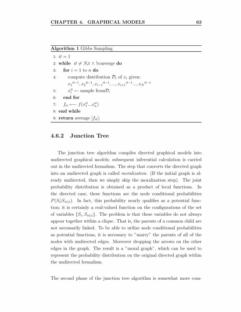
CHAPTER 4. GRAPHICAL MODELS 63
Algorithm 1 Gibbs Sampling
1: it = 1
2: while it 6= Nit ∧ !converge do
3: for i = 1 to n do
4: compute distribution Di of xi given:
x1it−1, x2
it−1, xi−1it−1, ..., xi+1
it−1..., xNit−1
5: xiti ← sample fromDi
6: end for
7: fit ←− f(xit1 ...x
itn )
8: end while
9: return average [fit];
4.6.2 Junction Tree
The junction tree algorithm compiles directed graphical models into
undirected graphical models; subsequent inferential calculation is carried
out in the undirected formalism. The step that converts the directed graph
into an undirected graph is called moralization. (If the initial graph is al-
ready undirected, then we simply skip the moralization step). The joint
probability distribution is obtained as a product of local functions. In
the directed case, these functions are the node conditional probabilities
P (Si|Sπ(i)). In fact, this probability nearly qualifies as a potential func-
tion; it is certainly a real-valued function on the configurations of the set
of variables {Si, Sπ(i)}. The problem is that these variables do not always
appear together within a clique. That is, the parents of a common child are
not necessarily linked. To be able to utilize node conditional probabilities
as potential functions, it is necessary to ”marry” the parents of all of the
nodes with undirected edges. Moreover dropping the arrows on the other
edges in the graph. The result is a ”moral graph”, which can be used to
represent the probability distribution on the original directed graph within
the undirected formalism.
The second phase of the junction tree algorithm is somewhat more com-

CHAPTER 4. GRAPHICAL MODELS 64
plex. This phase, known as triangulation, takes a moral graph as input
and produces as output an undirected graph in which additional edges have
(possibly) been added. This latter graph has a special property that allows
recursive calculation of probabilities to take place. In particular, in a trian-
gulated graph, it is possible to build up a joint distribution by proceeding
sequentially through the graph, conditioning blocks of interconnected nodes
only on predecessor blocks in the sequence.
A graph is not triangulated if there are, for example, the cycle of four
nodes which do not have a chord, where a chord is an edge between non-
neighboring nodes. More generally, once a graph has been triangulated it
is possible to arrange the cliques of the graph into a data structure known
as a junction tree. A junction tree has the running intersection property: If
a node appears in any two cliques in the tree, it appears in all cliques that
lie on the path between the two cliques. This property has the important
consequence that a general algorithm for probabilistic inference can be based
on achieving local consistency between cliques. (That is, the cliques assign
the same marginal probability to the nodes that they have in common). In a
junction tree, because of the running intersection property, local consistency
implies global consistency. The probabilistic calculations that are performed
on the junction tree involve marginalizing and rescaling the clique potentials
so as to achieve local consistency between neighboring cliques. The time
complexity of performing this calculation depends on the size of the cliques;
in particular for discrete data the number of values required to represent the
potential is exponential in the number of nodes in the clique. For efficient
inference, it is therefore critical to obtain small cliques.

Chapter 5
Representation of the crystal
structure with graphical
models
Structural knowledge can help explaining not only the behavior of individual
molecules, but also grasping the type and nature of DNA-protein or protein-
protein interactions.
A lot of work has been dome to describe the physical interactions occur-
ring between transcription factors and their cis-acting element located on
DNA. One of the best type of data that better describe the interaction be-
tween molecules are the crystal structures, see Section 2.6 for mode details.
As of November 2007 there were over 800 structures of transcription factors
available in the Protein Data Bank (PDB) [8] 1, and approximately 200 of
them are co-structure with small fragments of DNA or RNA. [60]. Analysis
of the protein-DNA complexes has shown that recognition of DNA or RNA
is usually achieved using a limited number of structural motifs.
Specific sequence recognition is mainly achived by interaction of the
motif via the DNA major groove and these interactions can be stabilized by
other interactions encompassing DNA backbone or minor groove. Several
Transcriptional Factors (TF) contain multiple copies of zinc fingers, allowing
1The PDB is the single worldwide repository for the processing and distribution of
3-D structure data of biological molecules and complexes.

CHAPTER 5. REPRESENTATION OF THE CRYSTALSTRUCTURE WITH GRAPHICAL MODELS 66
the recognition of longer stretches of the DNA sequence, thus achieving
greater specificity. Other popular motifs are the helix-turn-helix and leucine
zipper, it is possible to find more details in Section 2.5.2 .
Large biomolecules such as proteins, DNA and RNA tend to be dynamic
entities, constantly in motion. In addition to their thermal vibrations and
rotations these molecules can exhibit a range of other motions, often associ-
ated with their function, including bending, twisting, opening, closing and
movements of side chains, loops, flaps and domains.
Let us consider the case of typical DNA binding protein characterized by
a binding site of about ten base pairs in length. There are over 106 possible
sequences for a 10 bases site. Furthermore, if the protein uses 10 amino acid
residues to recognise its DNA target, then the number of possible residues
is 2010. Therefore, a table encompassing all the affinity values would be
made by more than 1019 values.
Since it is not practical to perform such huge number of experiments, we
use graphical models to obtain a more realistic approach to determine a
good way to capture the variability of the interactions between nucleotides
and amino acids. The graphical models allow to infer the best binding motif
in a family of transcriptional factors.
In Section 3.1 we described the two main ways used to represent TFBSs.
The most commonly used representation of TFBSs is the position weight
matrix (PWM). This matrix contains a score for all possible bases at each
position in the binding site. PWMs are a good way to represent a TFBS
since they can capture the variability of different TFBSs obtained from
biological experiment.
However, all existing algorithms that build the PWMs assume each nu-
cleotide in a DNA sequence as independent from the others. Under such
assumption their log independence model turns to be an additive one.
However, the independent assumption does not represent the real sit-
uation of dependencies in a DNA-protein interaction where the same nu-
cleotide can interact with two or more, different amino acids and individual
CHAPTER 5. REPRESENTATION OF THE CRYSTALSTRUCTURE WITH GRAPHICAL MODELS 67
amino acid may interact with more then one base.
The inadequacy of such representation is showed, for instance, in Bulyk’s
paper [52]. Bulyk et al. studied the protein-DNA interactions of the
wild-type mouse EGR1 zinc finger protein and four mutants with amino
acid substitutions in the middle finger. Using microarray technology, they
measured the DNA-binding affinity of the five proteins to 10mer targets
encompassing all 64 possible trinucleotides in their central positions, i.e.
those that interact directly with the middle finger according to the co-
crystal structure. From this analysis they concluded that each nucleotide in
the binding site does not contribute independently to the binding affinity,
and a dinucleotide model provides a better fit compared to a simple additive
model.
Initially, the first mathematical model that we considered to represent
DNA-protein interactions has been a Pair Hidden Markov Model (PHMM) [19].
PHMM is an extension of HMM [19], where the observations are formed by
a couple of sequences and the model assumes that the hidden alignment
sequence is a Markov chain that determines the probability distribution of
the observations. Figure 5.1(A) shows a PHMM, where each state emits
either a residue or a gap for both sequences. Using this formalism, the out-
put is made of sorted couples of bases which form two aligned sequences.
As shown in Figure 5.1(B), the PHMM formalism only models interaction
among two sequences in a linear and consecutive way, because the key prop-
erty of a Markov chain is that the probability of each position depends only
on the value of the preceding position, not on the entire previous sequence.
However, evidence from few crystal structures showed that links among
DNA and protein are “intertwisted”. Following this assumption, the situa-
tion that we would like to represent is that shown in Figure 5.1(C) Inter-
wisted interaction can not be represented by pairHMM for the key Markov
property if the Markov chain is not anymore satisfied. In fact the emission
of symbol couples means a hidden links among them, but this is not always
true. We need a formalism that allow to model more complex and crossed
links as shown in Figure 5.1(C). Moreover if we increase the number of state
of PHMM, where each state represent a link in the crystal structure we have
the state space explosion problem. Instead using the graphical models pro-

CHAPTER 5. REPRESENTATION OF THE CRYSTALSTRUCTURE WITH GRAPHICAL MODELS 68
Figure 5.1: PairHMM. A PairHMM can generate two sequences at the same
time according to model shown in (A). The rectangles represent state emit-
ting residues for one or both sequences. (B) Output of a typical PairHMM,
the symbol with the same colour are emitting at the same time. This means
a link among these bases. (C) The situation that we want to represent,
where the links among the bases have crossed each other; and that can not
be represented by a Markov model due to its memory property.

CHAPTER 5. REPRESENTATION OF THE CRYSTALSTRUCTURE WITH GRAPHICAL MODELS 69
posed in this thesis, allows the representation of sequences interacting in a
intertwisted manner, they provide a concise language for describing prob-
ability distributions over the observations. The graphical models proposed
in this thesis to represent such interactions are MRF and BN.
Our goal is to determine a model of DNA-protein interactions in terms of:
the atom type, atomic coordinates, and other experimental parameters that
improve the description of the DNA protein interactions. Our methodology
can be applied to every type of crystal structure representing an interaction
between DNA and proteins. In order to estimate distribution frequencies
of nucleotide and amino acids involved in all possible interactions we have
integrated the data from crystal structure with experimental data from
SELEX and phage display.
Our development strategy consists of three main steps:
• Links identification. Links identification denotes the problem of deter-
mining the interactions between proteins and DNA. Three techniques
namely distance, HBPLUS and JRP were used to identify hydrogen
bonds and Van der Waals contacts involved in the interaction of amino
acid residues and water molecules with DNA atoms.
• Graphical model construction. MRF and BN are used to build two
models representing DNA-proteins links previously identified.
• Inference. For each model we exploit the inference algorithms to pre-
dict the DNA sequence given a protein. Even though we are not
explicitly interested in the reverse inference problem, i.e. predicting
protein sequence given DNA sequence, the model would support this
inference without further modifications.
5.1 Links identification
There are two main types of interactions between protein and DNA: hy-
drogen bonds and van der Waals contacts. Van der Waals contacts exist if
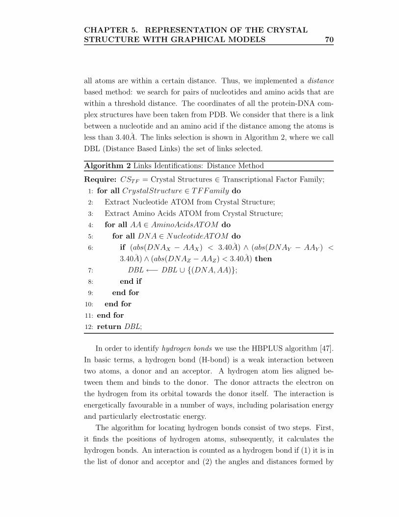
CHAPTER 5. REPRESENTATION OF THE CRYSTALSTRUCTURE WITH GRAPHICAL MODELS 70
all atoms are within a certain distance. Thus, we implemented a distance
based method: we search for pairs of nucleotides and amino acids that are
within a threshold distance. The coordinates of all the protein-DNA com-
plex structures have been taken from PDB. We consider that there is a link
between a nucleotide and an amino acid if the distance among the atoms is
less than 3.40A. The links selection is shown in Algorithm 2, where we call
DBL (Distance Based Links) the set of links selected.
Algorithm 2 Links Identifications: Distance Method
Require: CSTF = Crystal Structures ∈ Transcriptional Factor Family;
1: for all CrystalStructure ∈ TFFamily do
2: Extract Nucleotide ATOM from Crystal Structure;
3: Extract Amino Acids ATOM from Crystal Structure;
4: for all AA ∈ AminoAcidsATOM do
5: for all DNA ∈ NucleotideATOM do
6: if (abs(DNAX − AAX) < 3.40A) ∧ (abs(DNAY − AAY ) <
3.40A) ∧ (abs(DNAZ −AAZ) < 3.40A) then
7: DBL ←− DBL ∪ {(DNA,AA)};
8: end if
9: end for
10: end for
11: end for
12: return DBL;
In order to identify hydrogen bonds we use the HBPLUS algorithm [47].
In basic terms, a hydrogen bond (H-bond) is a weak interaction between
two atoms, a donor and an acceptor. A hydrogen atom lies aligned be-
tween them and binds to the donor. The donor attracts the electron on
the hydrogen from its orbital towards the donor itself. The interaction is
energetically favourable in a number of ways, including polarisation energy
and particularly electrostatic energy.
The algorithm for locating hydrogen bonds consist of two steps. First,
it finds the positions of hydrogen atoms, subsequently, it calculates the
hydrogen bonds. An interaction is counted as a hydrogen bond if (1) it is in
the list of donor and acceptor and (2) the angles and distances formed by

CHAPTER 5. REPRESENTATION OF THE CRYSTALSTRUCTURE WITH GRAPHICAL MODELS 71
the atoms surrounding the hydrogen bond satisfy a fixed set of constraints.
If the donor (D) and acceptor (A) are only one or two covalent bonds apart,
the interaction is not counted as a hydrogen bond. The set of constraints
exploited by HBPLUS are shown in Algorithm 3, where we call HL (H
Links) the set of links selected.
Algorithm 3 Links Identifications: HBPLUS
Require: Crystal Structure
1: N = { Set of atoms neighboring H in the Crystal Structure};
2: for all Ni ∈ N do
3: for all Nj ∈ N do
4: FirstCheck =∧
coord∈x,y,z
|Hcoord −Nicoord| < 2.7A
5: SecondCheck =∧
coord∈x,y,z
|Nicoord−Njcoord
| < 3.35A
6: ThirdCheck = angle(Nj −Ni −H) > 90◦
7: FourthCheck = angle(Nj − AA−H) > 90◦
8: if FirstCheck ∧ SecondCheck ∧ ThirdCheck ∧ FourthCheck
then
9: HL ←− HL ∪ {(Nj, Ni)}
10: end if
11: end for
12: end for
13: return HL;
To refine the detected links chosen we perform a Mutual Information
analysis (MI) using the Master alignment of binding sites described by
Gutell at al. [61], identifying co-variant positions on the mutual informa-
tion observed between them. Given an alignment of multiple sequences, we
wish to determine the degree of covariation between two positions x and
y. We begin by determining the frequency at which every base occurs at
every positions, fbx and fby, where b ∈ (A, T, C,G). We also determine the
frequencies of the pairs of bases occurring at positions x and y in the same
sequence, fbxby. If the two positions vary independently of one another
then fbxby ≈ fbx×fby, and we measure the divergence from independence.
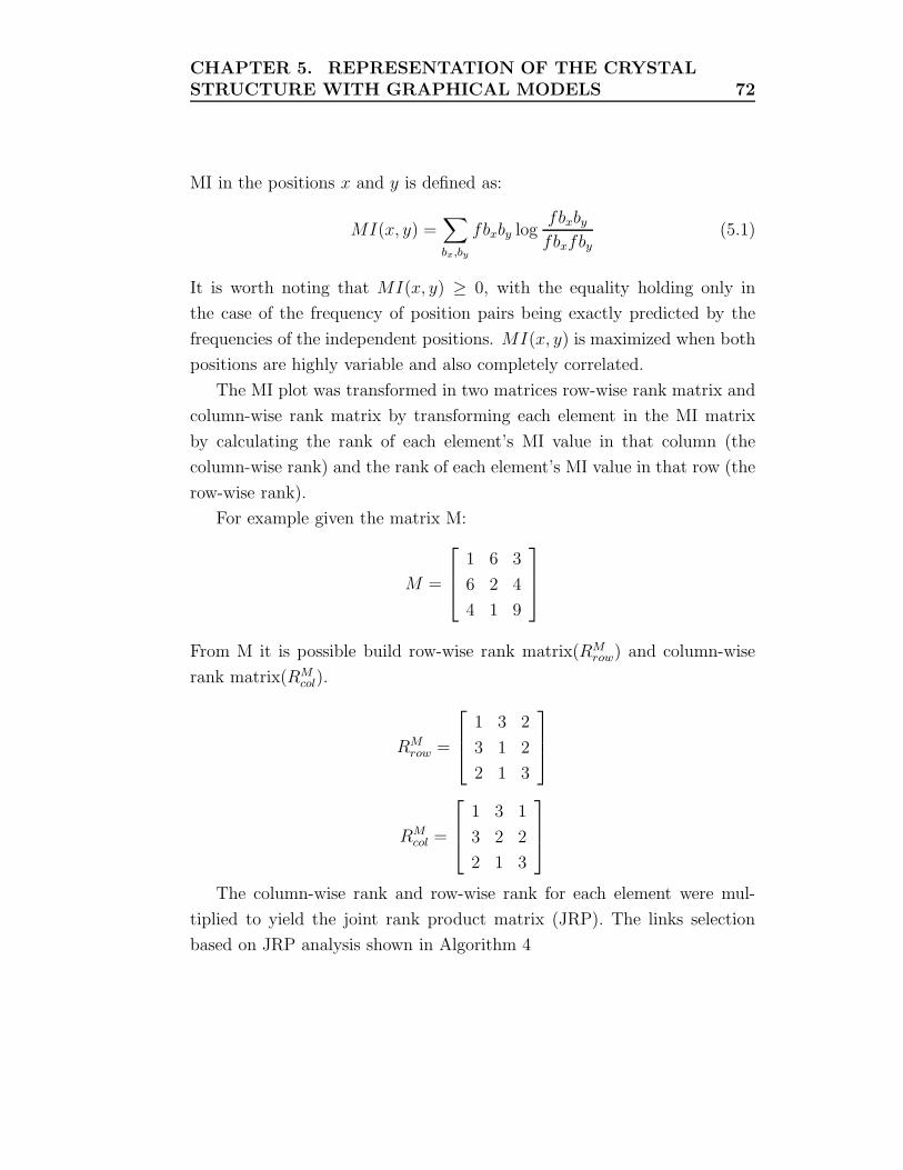
CHAPTER 5. REPRESENTATION OF THE CRYSTALSTRUCTURE WITH GRAPHICAL MODELS 72
MI in the positions x and y is defined as:
MI(x, y) =∑
bx,by
fbxby logfbxbyfbxfby
(5.1)
It is worth noting that MI(x, y) ≥ 0, with the equality holding only in
the case of the frequency of position pairs being exactly predicted by the
frequencies of the independent positions. MI(x, y) is maximized when both
positions are highly variable and also completely correlated.
The MI plot was transformed in two matrices row-wise rank matrix and
column-wise rank matrix by transforming each element in the MI matrix
by calculating the rank of each element’s MI value in that column (the
column-wise rank) and the rank of each element’s MI value in that row (the
row-wise rank).
For example given the matrix M:
M =
1 6 3
6 2 4
4 1 9
From M it is possible build row-wise rank matrix(RMrow) and column-wise
rank matrix(RMcol).
RMrow =
1 3 2
3 1 2
2 1 3
RMcol =
1 3 1
3 2 2
2 1 3
The column-wise rank and row-wise rank for each element were mul-
tiplied to yield the joint rank product matrix (JRP). The links selection
based on JRP analysis shown in Algorithm 4

CHAPTER 5. REPRESENTATION OF THE CRYSTALSTRUCTURE WITH GRAPHICAL MODELS 73
Algorithm 4 Links Identifications: MI and JRP
Require: SDNA, SAA = sequences interact between them;
1: MI = matrix of SDNA.length rows and SAA.length columns;
2: X = element wise product;
3: for i = 0 to SDNA.length do
4: for j = 0 to SAA.length do
5: MI(i, j) as specified in 5.1
6: end for
7: end for
8: JRP = matrix of SDNA.length rows and SAA.length columns;
9: JRP = RMIrow X RMI
col
10: return JRP ;
We have manually assigned a score to every potential link found by
either distance, HBPLUS, or JRP. First we considered only the links for
which two out of the three methods agree. We calculate, for each links,
the average number of occurrences in the set of crystal structures that we
analyzed. The set of constraints that we applied in order to determine a
score are:
• the values of JRP minus a threshold.
• the average number of occurrences are greater than 1
• the link is recognized as “canonical” link in the protein family that
we analyze.
5.2 Graphical model construction
Graphical model attributes are usually either given by some domain expert
or learned from data. In this work, we do not follow this path. Instead,
our strategy consists in using data from “crystallography experiments” as
graphical templates for our models. Further experimental evidence is then
used in order to induce the probabilities distributions associated to the
graphs obtained in this way.
CHAPTER 5. REPRESENTATION OF THE CRYSTALSTRUCTURE WITH GRAPHICAL MODELS 74
In order to understand our implementation it is useful to refer to Fig-
ure 5.2 where there are reported set of links characterizing Zif 268-DNA
(PDB code: 1a1f). Nucleotides are represented by one letter codes and are
coloured according to their type. Nucleotides pairs are connected by a solid
black line between them. The DNA backbones are drawn next to the bases:
the sugar are represented as light blue pentagons and phosphates as purple
circles. The base numbers, as given in the canonical numeration for Zinc
Finger protein, are written inside the sugar. Interactions are plotted on
either side of the strands; interacting protein residues are represented by
residue name and number.
The rest of this section details the design choices we made to implement
the structural information crystal structure in graphical models.
Markov Random Fields
The the first step in building a MRF is the choice of the model structure.
We represent the interaction between DNA and protein using a graph
G = (V, E) where vertices of the graph represent nucleotides (we will refer
to them as DNA vertices) and amino acid positions (that we will refer to
them as AA vertices) and edges represent interactions between residues.
We will assign to each vertex in the graph one of a finite set∑
of
labels. Since we have two types of vertices we also have two finite sets
of labels and two different alphabets. The alphabet associated to DNA
vertices is∑
D = A, T, C,G, while the alphabet associated to AA vertices
is∑
A = A,R,N,D,C,E,Q,G,H, I, L,K,M, F, P, S, T,W, Y, V .
Let us consider Figure 5.3. where we have shown the model structure
that we obtain representing the direct links between DNA nucleotides and
protein amino acids. This model best reflects the dependencies known to
exists in the 1a1f crystal structure. Since we model a structural vision of
DNA-protein interactions this is a model that best reflects the dependencies
in the biological domain.
However, in order to be complete, this model we also require the addi-
tion of the direct links existing among nucleotides and among amino acids.
Moreover, biological observations suggest that there are interactions also
among not adjacent positions of nucleotides and amino acids. The resulting

CHAPTER 5. REPRESENTATION OF THE CRYSTALSTRUCTURE WITH GRAPHICAL MODELS 75
Figure 5.2: A diagram of the Zif 268-DNA complex

CHAPTER 5. REPRESENTATION OF THE CRYSTALSTRUCTURE WITH GRAPHICAL MODELS 76
Figure 5.3: Model that reflects the dependencies known to exists in DNA-
Zif268 complex.

CHAPTER 5. REPRESENTATION OF THE CRYSTALSTRUCTURE WITH GRAPHICAL MODELS 77
Figure 5.4: Graph with a complete biological knowledge
model structure is reported in Figure 5.4.
Unfortunately, the complexity of estimating the MAP assignment (as
defined in Section 4.6) on the graph is exponential in the size of the largest
clique of the graph. [In some cases it is possible to exploit the special form
of potential to design optimal MAP algorithms like the mincut algorithm
for associative potentials. However this type of algorithm suggests binary
labels, but we have two alphabet label sets with four and twenty elements
respectively]. This implies that even though the model in Figure 5.4 is
more precise from a biological perspective, its implementation would require
computational resources beyond those at our disposal. As a compromise we
decided to implement the graphical model reported in Figure 5.5.
Here, due to the fact that we want to infer on DNA binding sites rather
than on amino acids, we decided to eliminate the links between the amino
acids positions. In this way, on one side we drastically reduce the computa-
tional resources needed to work with the model, while on the other side we

CHAPTER 5. REPRESENTATION OF THE CRYSTALSTRUCTURE WITH GRAPHICAL MODELS 78
Figure 5.5: MRF Topology graph in implementation of Zif268-DNA inter-
actions
do not lose information about the dependencies between DNA positions.
Once the structure is fixed, we still need to find a proper potential
function. More specifically we must assign a value ψC(ωC) > 0 to every
subconfiguration ωC of a configuration ω, where C ranges on the set of all
cliques of G.
By theorem 2 (Hammersley-Clifford): every choice of potentials, ψC(ω)
such that ∀ψC(ωC), ∀ω : ψC(ωC) > 0 induces a probability distribution that
is a MRF with respect to graph G.
We choose the values of ψC(ωC) based on the frequencies of the joint
probability of the bases that are involved in the same clique. i.e. ψC(ωC) =
freq(ωC) in a separate experimental dataset. To obtain the frequencies
of different nucleotides and amino acids involved in the links we must use
different data sets, to since in PDB there are not sufficient replicates of

CHAPTER 5. REPRESENTATION OF THE CRYSTALSTRUCTURE WITH GRAPHICAL MODELS 79
the same crystal structure. Using experimental data from SELEX or phage
display we can also obtain an indirect measurement of the binding affinity
of the protein and its mutants to particular DNA targets. These values are
not a real measure of affinity, however the frequency should be related to
the affinity.
Since ψC(ωC) is required to be strictly positive, when freq(ωC) = 0 we
set ψC(ωC) to the Laplace distribution [53].
Bayesian Network
In order to compare the results obtained from MRF with another graph-
ical model we have implemented a Bayesian Network (Section 4.4), an al-
ternative approach to describe the links in DNA protein interaction.
BNs are models based on a directed graph G = (V, E), where verticies,
as in MRF, represent DNA and amino acid positions and edges represent
the links among bases. The topology of our BN is represented in Figure 5.6
where links from DNA and protein have been selected using the technique
explained in Section 5.1.
Since BNs are directed models, if an arrow connects node A to node B,
this means that A influences the output of B, but not viceversa.
Defining a direction is hard since nucleotides and amino acids influence
each other.
We arbitrarily decided to model influences from protein amino acids to
DNA nucleotides since this is the directionality that best fulfills our purpose.
While this choice is far from optimal it is, from our point of view, the most
sensible one. The difficulty in creating a coherent BN is indeed an indicator
that MRF are better suited for the task at hand since are biological intuitive.
This direction is intuitive when we consider the type of inference that we
want to perform: given a protein sequence, we ask which are the highest
affinity DNA sequences that produce such a sequence.
In defining a BN, one needs to define the conditional probability distri-
butions associated to each node. In our approach we estimate such distri-
bution from a separate dataset using an approach similar to what we did

CHAPTER 5. REPRESENTATION OF THE CRYSTALSTRUCTURE WITH GRAPHICAL MODELS 80
Figure 5.6: BN Topology graph in implementation of Zif268-DNA interac-
tions

CHAPTER 5. REPRESENTATION OF THE CRYSTALSTRUCTURE WITH GRAPHICAL MODELS 81
for MRF ψC function.
Following standard practices in BN, it is necessary to use a prior distri-
bution to any possible configuration of values. Using frequencies extracted
from experimental data sets we have the same problem that occurs in MRF,
we do not observe all possible combinations of nucleotides and amino acids
in the interacting positions. To overcome this problem we have used Laplace
correction [53].
−−
In the previous Section of this chapter we have explained in details the
design choices we made to implement the MRF and BN from crystal struc-
tures. In order to obtain a good model we decided to partition the crystal
structures by family of transcriptional factors they represent. We need to
classify TFs into classes so that TFs with similar DNA-binding domains are
grouped together. For this purpose, we use the TRANSFAC database [73].
TRANSFAC is a publicly accessible database that maintains a comprehen-
sive list of eukaryotic TFs, along with their structural domains and the
sequences to which they are known to bind. TRANSFAC organizes TFs in
a hierarchy; at the top level, there are four families: zinc-coordinating, basic
domains, helix-turn-helix and beta scaffold. Each family is further divided
into a larger number of classes.
Given a family, we extract from the PDB database all the crystal struc-
tures of proteins of that family and containing that complex.
Once all relevant crystal structures have been found, there exist at least
two ways to build a graphical model based on them:
• Single comprehensive. Build a unique model that describes the whole
family of TFs.
• One model per structure Build a model from each crystal structure
belonging to a specific TF family.
In order to implement the first method, one would have to find a way to
align all the PDB entries that are present in the same family. Unfortunately,
this is a difficult process since the TF in crystal structures have different

CHAPTER 5. REPRESENTATION OF THE CRYSTALSTRUCTURE WITH GRAPHICAL MODELS 82
orientations. Moreover, if we consider a family of Zinc Finger Cys2His2,
the crystal structure also contain a different number of zinc finger. This
constrains establish a difficult environment from which extracting a unique
model.
In our approach, we follow the second way, we build for every crystal
structure, belonging to the same family, a separate graphical model.
5.3 Inference
The models so constructed embed knowledge about a given interaction do-
main.Given the observations for all (or some) AA vertexes, we can infer on
DNA sequences that can link to the protein.
We perform the chosen inference algorithms on each graphical model
that we implement: Gibbs samplig algorithm on MRF and Junction Tree
on BN. Since we want to obtain transcriptional factor binding sites that
summarize the interaction characteristics of a specific TF family.
We perform inference stating from the graphical models on each family
of TF. The output of the inference algorithms is a probability distribution
of DNA labels for each DNA vertex present in the model.
If a DNA vertex is present only in one crystal structure we have only one
probability distribution that we assign to that specific vertex. If the DNA
vertex is present in more structures we must to combine these probability
distributions in order to obtain a unique distribution on the four nucleotides.
We now consider three ways to combine the probability distributions
and explain why the third is the most satisfactory.
majority voting : for each distribution, we replace the largest probability
by 1 and the others by 0s; then, we sum the values for each nucleotide
and divide by the number of sequences. In other words, we assign to each
nucleotide a probability equal to the fraction of distributions in which it has
the largest probability. The limit of this procedure is that, if a nucleotide
does not have the largest probability in all distributions, then we retain no
information about it. Since we want a probability for every nucleotides, we
dismiss this method.
sum and mean: for each nucleotide, we sum the probabilities assigned by

CHAPTER 5. REPRESENTATION OF THE CRYSTALSTRUCTURE WITH GRAPHICAL MODELS 83
each distribution, then we divide the result by the number of distributions.
In other words, we assign to each nucleotide the mean probability it is
assigned by the distributions. This method is more informative than the
first, but too sensitive to outliers.
weighted arithmetic mean: we divide the probability values of each nu-
cleotide by the number of sequences and we sum these values. In this way
each probability values is weighted using the frequency of each appears in
each sequences. we weighted every value with respect to its frequency and
obtain a value that reflects all distributions.
Chapter 6
Results
The focus of the presented work is the definition of TFBS structure on the
basis of protein-DNA interaction data. Specially we focus our experiments
on the DNA-protein interactions for a specific family of transcription fac-
tors(TFs) even thought we can use this method on all TFs family. We built
a model in such way that it can summarize the common features between
the transcriptional factors in the same family but also pick up the links that
characterize also a single TF.
To test our methodology we implemented both graphical models on a
zinc finger family of transcriptional factors the Zinc finger, Cystein 2 His-
tine 2 (Cys2His2). Zinc-coordinating proteins represent up the largest single
group of TF in eucaryotic genomes, and the DNA-binding motif is charac-
terized by the tetrahedral coordination of one or two zinc ions by conserved
cysteine (C) and histidine (H) residues (Figure 6.1). The widespread use of
this arrangement is believed to be due to the structural stability the metal
ions offer to domains that have not a hydrophobic core large enough to
stabilize the domain structure.
Protein subunits often contain multiple fingers that wrap around the
DNA in a spiral manner. Fingers bind adjacent 3 bases subsites by inserting
the α helix in the major groove, and the recognition pattern between the
helix and DNA is well characterized. Amino acids at positions -1, 2, 3 and
6 relative to the start of the α helix are used to interact with the bases.
These are the links that we define “canonical”, Figure 6.1.
Our system is summarized by Figure 6.2. The first step is the extraction
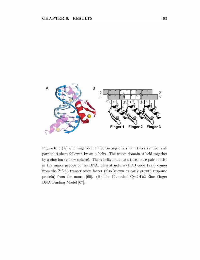
CHAPTER 6. RESULTS 85
Figure 6.1: (A) zinc finger domain consisting of a small, two stranded, anti
parallel β sheet followed by an α helix. The whole domain is held together
by a zinc ion (yellow sphere). The α helix binds to a three base-pair subsite
in the major groove of the DNA. This structure (PDB code 1aay) comes
from the Zif268 transcription factor (also known as early growth response
protein) from the mouse [60]. (B) The Canonical Cys2His2 Zinc Finger
DNA Binding Model [67].

CHAPTER 6. RESULTS 86
Figure 6.2: Pipeline of our strategy.
of crystal structures(first block in Figure 6.2), the main idea is to find which
positions in a protein sequence link to which positions in Transcription Fac-
tor Binding Site (TFBS). In a crystal structure these direct interactions are
known and we can determine which critical amino acid in this protein fam-
ily interacts with the DNA and its specific position in TFBS. To implement
the graphical model we map the interaction using edges and the nucleotides
and amino acids positions using vertices (second block in Figure 6.2), and,
our aim is to learn a different set of nucleotide and amino acids recogni-
tion preference for each of the vertices present in the model. To be able
to use our model like predictor, ie. given the observation (fourth block in
Figure 6.2) for all or some AA verticies, we can infer on DNA sequences
that the protein link, a set of frequencies (third block in Figure 6.2) as to be
determined for every possible configuration of values in each links position.
Following this pipeline we will go to explain in details the realization of
each block.
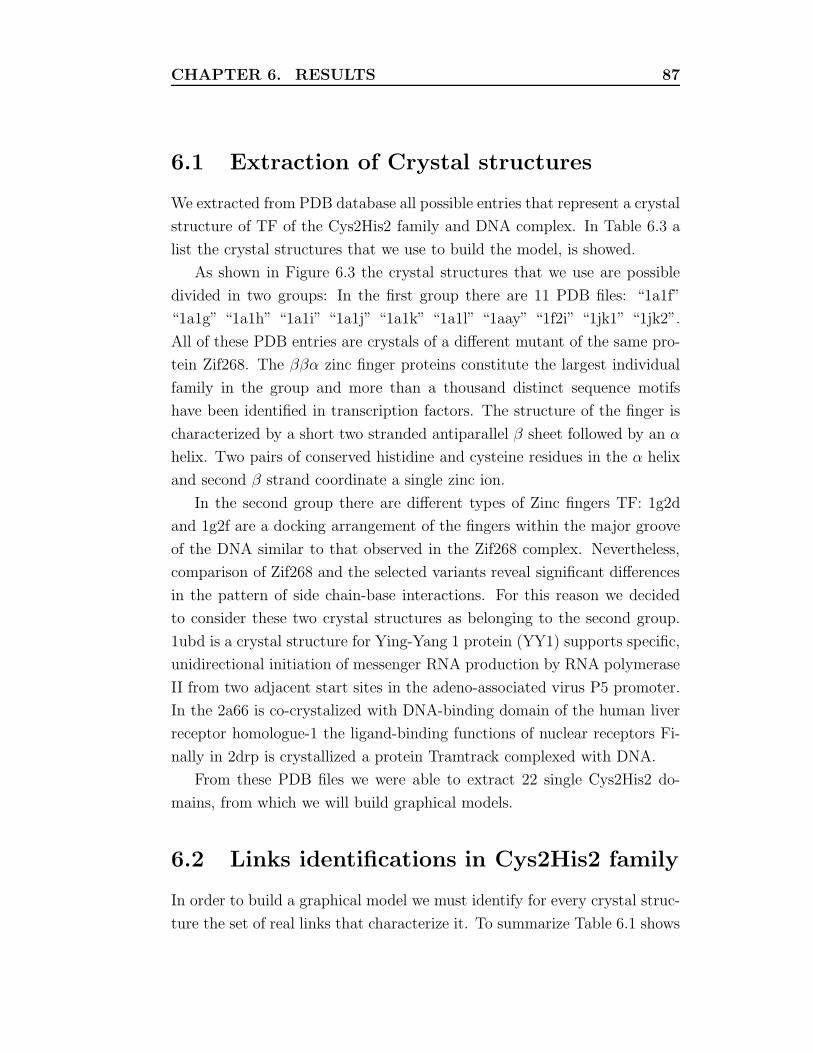
CHAPTER 6. RESULTS 87
6.1 Extraction of Crystal structures
We extracted from PDB database all possible entries that represent a crystal
structure of TF of the Cys2His2 family and DNA complex. In Table 6.3 a
list the crystal structures that we use to build the model, is showed.
As shown in Figure 6.3 the crystal structures that we use are possible
divided in two groups: In the first group there are 11 PDB files: “1a1f”
“1a1g” “1a1h” “1a1i” “1a1j” “1a1k” “1a1l” “1aay” “1f2i” “1jk1” “1jk2”.
All of these PDB entries are crystals of a different mutant of the same pro-
tein Zif268. The ββα zinc finger proteins constitute the largest individual
family in the group and more than a thousand distinct sequence motifs
have been identified in transcription factors. The structure of the finger is
characterized by a short two stranded antiparallel β sheet followed by an α
helix. Two pairs of conserved histidine and cysteine residues in the α helix
and second β strand coordinate a single zinc ion.
In the second group there are different types of Zinc fingers TF: 1g2d
and 1g2f are a docking arrangement of the fingers within the major groove
of the DNA similar to that observed in the Zif268 complex. Nevertheless,
comparison of Zif268 and the selected variants reveal significant differences
in the pattern of side chain-base interactions. For this reason we decided
to consider these two crystal structures as belonging to the second group.
1ubd is a crystal structure for Ying-Yang 1 protein (YY1) supports specific,
unidirectional initiation of messenger RNA production by RNA polymerase
II from two adjacent start sites in the adeno-associated virus P5 promoter.
In the 2a66 is co-crystalized with DNA-binding domain of the human liver
receptor homologue-1 the ligand-binding functions of nuclear receptors Fi-
nally in 2drp is crystallized a protein Tramtrack complexed with DNA.
From these PDB files we were able to extract 22 single Cys2His2 do-
mains, from which we will build graphical models.
6.2 Links identifications in Cys2His2 family
In order to build a graphical model we must identify for every crystal struc-
ture the set of real links that characterize it. To summarize Table 6.1 shows
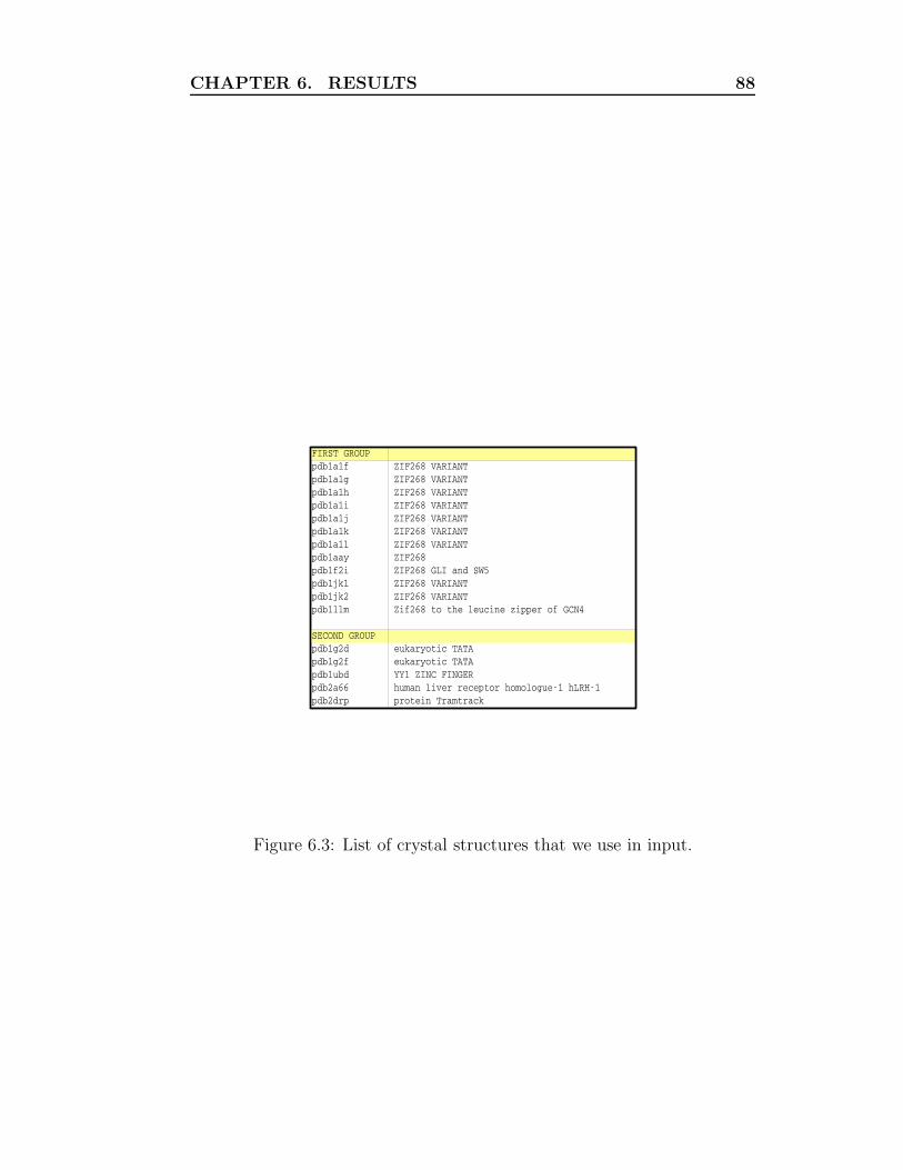
CHAPTER 6. RESULTS 88
Figure 6.3: List of crystal structures that we use in input.
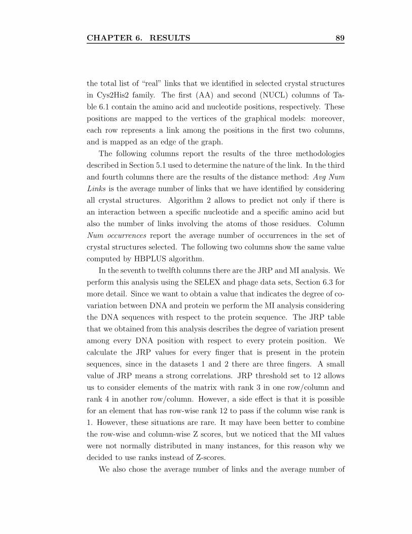
CHAPTER 6. RESULTS 89
the total list of “real” links that we identified in selected crystal structures
in Cys2His2 family. The first (AA) and second (NUCL) columns of Ta-
ble 6.1 contain the amino acid and nucleotide positions, respectively. These
positions are mapped to the vertices of the graphical models: moreover,
each row represents a link among the positions in the first two columns,
and is mapped as an edge of the graph.
The following columns report the results of the three methodologies
described in Section 5.1 used to determine the nature of the link. In the third
and fourth columns there are the results of the distance method: Avg Num
Links is the average number of links that we have identified by considering
all crystal structures. Algorithm 2 allows to predict not only if there is
an interaction between a specific nucleotide and a specific amino acid but
also the number of links involving the atoms of those residues. Column
Num occurrences report the average number of occurrences in the set of
crystal structures selected. The following two columns show the same value
computed by HBPLUS algorithm.
In the seventh to twelfth columns there are the JRP and MI analysis. We
perform this analysis using the SELEX and phage data sets, Section 6.3 for
more detail. Since we want to obtain a value that indicates the degree of co-
variation between DNA and protein we perform the MI analysis considering
the DNA sequences with respect to the protein sequence. The JRP table
that we obtained from this analysis describes the degree of variation present
among every DNA position with respect to every protein position. We
calculate the JRP values for every finger that is present in the protein
sequences, since in the datasets 1 and 2 there are three fingers. A small
value of JRP means a strong correlations. JRP threshold set to 12 allows
us to consider elements of the matrix with rank 3 in one row/column and
rank 4 in another row/column. However, a side effect is that it is possible
for an element that has row-wise rank 12 to pass if the column wise rank is
1. However, these situations are rare. It may have been better to combine
the row-wise and column-wise Z scores, but we noticed that the MI values
were not normally distributed in many instances, for this reason why we
decided to use ranks instead of Z-scores.
We also chose the average number of links and the average number of

CHAPTER 6. RESULTS 90
Table 6.1: List of links that we extract from a complete set of crystal
structures belonging to the same family.

CHAPTER 6. RESULTS 91
Figure 6.4: 3D graph reporting the average number of links and the average
number of occurrences of a link. Each point is depicted in different colors
that correspond to different JRP values.
occurrences among the distance and HBPLUS methodologies present in
fourteenth and fifteenth columns, respectively, as information to determine
the nature of the links. This choice have been done since we observe that
there is a proportionality among it and JRP values. In fact we have cal-
culated the number of times each link was observed as well as the average
number of atoms involved in each link and we have compared these to the
minimum JRP values. If we consider the 3D graph reported in Figure 6.4,
it is possible to observe that the average number of links and the average
number of occurrences of a link can be used to separate some of the low
JRP links from the set of all observed links.
Since proteins that are similar should have similar HBPLUS results,
and proteins that are divergent may have “novel” HBPLUS links that are
real but which have low number of occurrences, we decided to take into
consideration also such links (with a low number of occurrences), so as to
be able to also build models for underrepresented links.
Table 6.1 shows all possible links that we extracted by analysing the
fingers belonging to one TF all together. If considered positions -1 in protein

CHAPTER 6. RESULTS 92
sequences it is possible observe that this position amino acid positions links
with 4 different nucleotide positions: 3, 6, 9 and 10. These four links are
not with the same amino acid at positions -1, but with different amino acid
coming from the three different fingers of the protein. Since the goal of this
theses is to create a tool that allows to build a model that summarizes all the
features in the DNA protein interaction in a specific TF family, we obtain
Table 6.1 from an analysis performed considering all zinc fingers present in
the protein.
6.3 Data sets
Since in PDB database, every crystal structure is present only once we have
not the possibility to create a set of frequencies from the same types of data.
To overcome this problem we decided to use datasets that are obtained
from other types of biological experiments, the mutagenesis experiments
that offer the creations of recombinant DNA-Protein library.
The data of this group of papers derived from in vitro selection experi-
ments, namely SELEX and phage display. In SELEX experiment a protein
of known sequence is used to select DNA target form a pool of randomised
oligonucleotides. This procedure usually yields more that one DNA tar-
get. In a phage display experiment, the reverse randomisation and selection
procedure applies. A recombinant DNA library is built from this data and
consists of variants of the cDNA sequences of a known DNA-binding protein.
The nucleotides that code for certain amino acid positions are randomised.
Upon expression, the polypeptides are displayed on the outer coat of the
phages. Thus, proteins can be selected that bind with high affinity to the
fixed DNA target.
Table 6.2 shown the selected paper of experimental data collected from
the literature by Ryan Christensen. From which extracted the frequencies
to use as training and test data set.
All the data sets present in literature are using the same type of biologi-
cal experiments but limited only on a reduced set of residues. In particular
these experiments only explore the “canonical” links. Figure 6.3 shows a
portion of the type of data we used: each row represent an interaction be-

CHAPTER 6. RESULTS 93
Type of Data First Author Reference
SELEX Benos [58]
Additional Phage Display Dreier2001 [17]
Dreier2005 [18]
Hurt2003 [36]
Meng2007 [48]
Segal1999 [64]
Quantitative Data Bae2003 [6]
Bulyk2002 [12]
Segal1999 [64]
Cornu2007 [14]
Dreier2001 [17]
Dreier2005 [18]
Hamilton1998 [34]
Hurt2003 [36]
Liu2001 [43]
Liu2005 [41]
Liu2005b [42]
Segal1999 [64]
Wolf1999 [74]
Zhang2000 [76]
Table 6.2: List of selected paper that we use in order to extract the data to
test our model
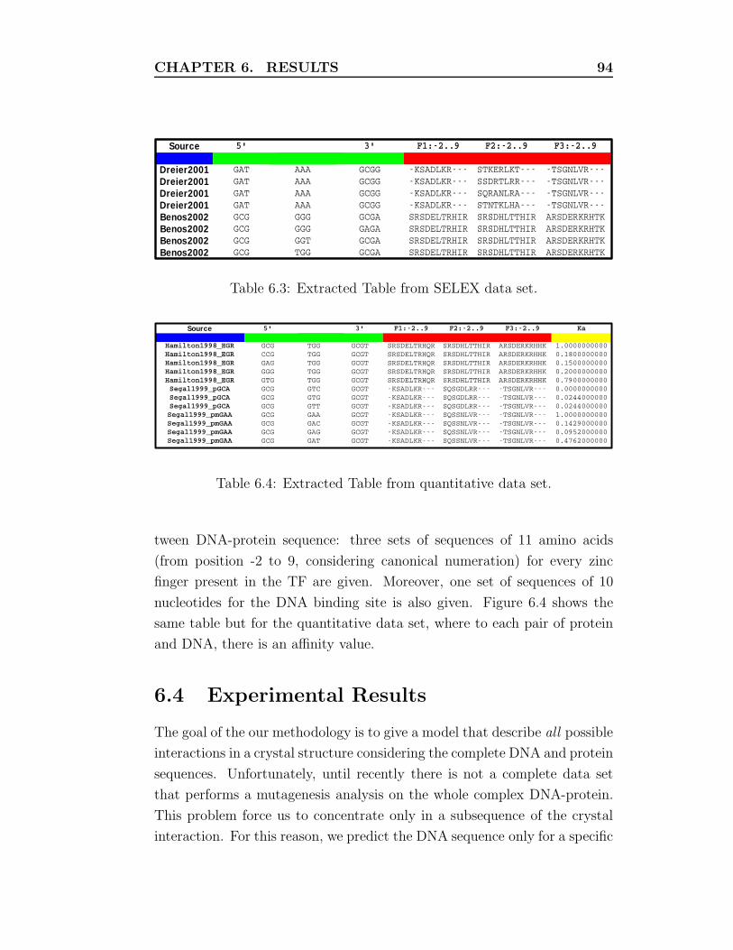
CHAPTER 6. RESULTS 94
Table 6.3: Extracted Table from SELEX data set.
Table 6.4: Extracted Table from quantitative data set.
tween DNA-protein sequence: three sets of sequences of 11 amino acids
(from position -2 to 9, considering canonical numeration) for every zinc
finger present in the TF are given. Moreover, one set of sequences of 10
nucleotides for the DNA binding site is also given. Figure 6.4 shows the
same table but for the quantitative data set, where to each pair of protein
and DNA, there is an affinity value.
6.4 Experimental Results
The goal of the our methodology is to give a model that describe all possible
interactions in a crystal structure considering the complete DNA and protein
sequences. Unfortunately, until recently there is not a complete data set
that performs a mutagenesis analysis on the whole complex DNA-protein.
This problem force us to concentrate only in a subsequence of the crystal
interaction. For this reason, we predict the DNA sequence only for a specific

CHAPTER 6. RESULTS 95
part of the DBD. Then, we decide to improve the performance of our method
combining the prediction that we obtain. In our approach, we build for every
crystal structure, belonging to the same family, many graphical models, one
for every zinc finger in the crystal structure.
In Section 5.3 we described the how to combine the probability distri-
butions obtained, from each graphical model, in order to provide a unique
distribution on the four nucleotides for every DNA vertex position. We re-
organized the distribution that we obtained extracting from each zinc finger
a set of column, more precisely, columns 1, 2 and 3 from Finger 3; columns
4, 5 and 6 from Finger 2 and columns 7, 8 and 9 from Finger1. This choice
it was performed following the canonical connection.
Even though there are many algorithms that search a TFBS in the
genome we can not compare our results with these methods. In fact the
assumptions that we impose in our methodologies, with respect to the other
works, are more different between each other. The strong assumption about
the structural dependencies between DNA and protein sequence is never
used before. Moreover the type of data that we obtain in output, even
though they are probability distributions associated to every DNA vertices,
we can not consider and then use them like a PWM.
First of all, we would like to test if the presented method is able to
distinguish between real TFBS and intergenic DNA. To do this we used a
set of TF sequences along with their TFBS sequences and computed a score
value that represents the binding probability. We also used the same TF
sequences against intergenic DNA sequences and computed the score values.
The score for any particular site is given by the product of the probability
values for every nucleotides in the site.
The score for each nucleotide at a given position is derived from the
combination of the probability distributions obtained from the inference
algorithms.
Figure 6.5 and Figure 6.6 plot the scores obtained from the graphical
models for true TFBS (solid line) against the scores of intergenic DNA
sequences (dash line).

CHAPTER 6. RESULTS 96
Figure 6.5: Graph of correlation of score obtained using real TFBS and
intergenic DNA sequences in MRF Models.
Figure 6.6: Graph of correlation of score obtained using real TFBS and
intergenic DNA sequences in BN Models.
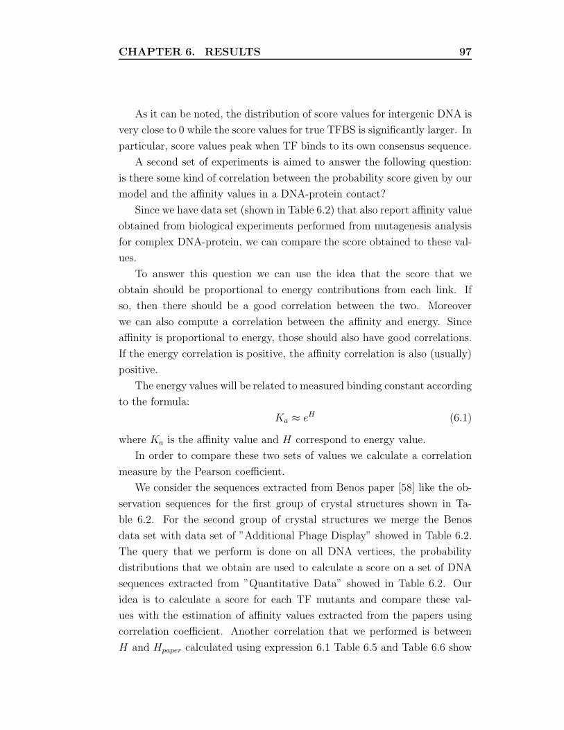
CHAPTER 6. RESULTS 97
As it can be noted, the distribution of score values for intergenic DNA is
very close to 0 while the score values for true TFBS is significantly larger. In
particular, score values peak when TF binds to its own consensus sequence.
A second set of experiments is aimed to answer the following question:
is there some kind of correlation between the probability score given by our
model and the affinity values in a DNA-protein contact?
Since we have data set (shown in Table 6.2) that also report affinity value
obtained from biological experiments performed from mutagenesis analysis
for complex DNA-protein, we can compare the score obtained to these val-
ues.
To answer this question we can use the idea that the score that we
obtain should be proportional to energy contributions from each link. If
so, then there should be a good correlation between the two. Moreover
we can also compute a correlation between the affinity and energy. Since
affinity is proportional to energy, those should also have good correlations.
If the energy correlation is positive, the affinity correlation is also (usually)
positive.
The energy values will be related to measured binding constant according
to the formula:
Ka ≈ eH (6.1)
where Ka is the affinity value and H correspond to energy value.
In order to compare these two sets of values we calculate a correlation
measure by the Pearson coefficient.
We consider the sequences extracted from Benos paper [58] like the ob-
servation sequences for the first group of crystal structures shown in Ta-
ble 6.2. For the second group of crystal structures we merge the Benos
data set with data set of ”Additional Phage Display” showed in Table 6.2.
The query that we perform is done on all DNA vertices, the probability
distributions that we obtain are used to calculate a score on a set of DNA
sequences extracted from ”Quantitative Data” showed in Table 6.2. Our
idea is to calculate a score for each TF mutants and compare these val-
ues with the estimation of affinity values extracted from the papers using
correlation coefficient. Another correlation that we performed is between
H and Hpaper calculated using expression 6.1 Table 6.5 and Table 6.6 show
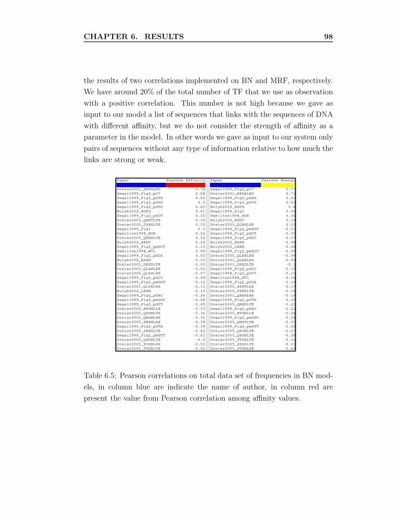
CHAPTER 6. RESULTS 98
the results of two correlations implemented on BN and MRF, respectively.
We have around 20% of the total number of TF that we use as observation
with a positive correlation. This number is not high because we gave as
input to our model a list of sequences that links with the sequences of DNA
with different affinity, but we do not consider the strength of affinity as a
parameter in the model. In other words we gave as input to our system only
pairs of sequences without any type of information relative to how much the
links are strong or weak.
Table 6.5: Pearson correlations on total data set of frequencies in BN mod-
els, in column blue are indicate the name of author, in column red are
present the value from Pearson correlation among affinity values.

CHAPTER 6. RESULTS 99
Table 6.6: Pearson correlations on total data set of frequencies in MRF
models, in column blue are indicate the name of author, in column red are
present the value from Pearson correlation among affinity values.
Then, we left out from the quantitative data one paper that we use as
test data the sequences listed in Bulyk’s paper [12], and used them as test
data. For every sequence of TFs we calculate the median value between the
affinity data, in this way we can discriminate the couple of sequences with
high (greater than median value) or low (less than median value) affinity.
We build a MRF and BN for this two set of sequences. The data reported in
Table 6.9 and Table 6.8 represent the results using BN.The data reported
in Table 6.10 and Table 6.7 represent the results using MRF. When we
build the graphical models with the positive training set means that our
models contain the features that allow the model to learn the structure of
DNA-protein complexes characterized by high values of affinity, shown in
Table 6.7 and Table 6.8.
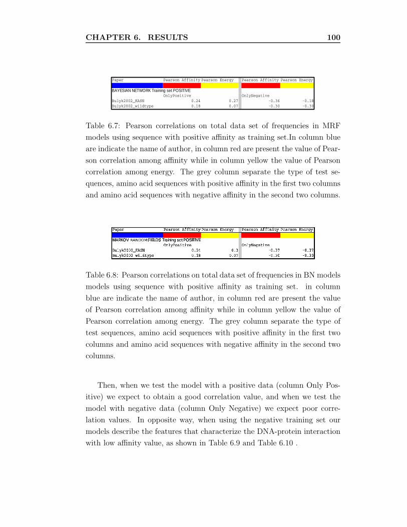
CHAPTER 6. RESULTS 100
Table 6.7: Pearson correlations on total data set of frequencies in MRF
models using sequence with positive affinity as training set.In column blue
are indicate the name of author, in column red are present the value of Pear-
son correlation among affinity while in column yellow the value of Pearson
correlation among energy. The grey column separate the type of test se-
quences, amino acid sequences with positive affinity in the first two columns
and amino acid sequences with negative affinity in the second two columns.
Table 6.8: Pearson correlations on total data set of frequencies in BN models
models using sequence with positive affinity as training set. in column
blue are indicate the name of author, in column red are present the value
of Pearson correlation among affinity while in column yellow the value of
Pearson correlation among energy. The grey column separate the type of
test sequences, amino acid sequences with positive affinity in the first two
columns and amino acid sequences with negative affinity in the second two
columns.
Then, when we test the model with a positive data (column Only Pos-
itive) we expect to obtain a good correlation value, and when we test the
model with negative data (column Only Negative) we expect poor corre-
lation values. In opposite way, when using the negative training set our
models describe the features that characterize the DNA-protein interaction
with low affinity value, as shown in Table 6.9 and Table 6.10 .

CHAPTER 6. RESULTS 101
Table 6.9: Pearson correlations on total data set of frequencies in BN mod-
els using sequence with negative affinity as training set. In column blue are
indicate the name of author, in column red are present the value of Pear-
son correlation among affinity while in column yellow the value of Pearson
correlation among energy. The grey column separate the type of test se-
quences, amino acid sequences with positive affinity in the first two columns
and amino acid sequences with negative affinity in the second two columns.
Table 6.10: Pearson correlations on total data set of frequencies in MRF
models using sequence with negative affinity as training set. In column
blue are indicate the name of author, in column red are present the value
of Pearson correlation among affinity while in column yellow the value of
Pearson correlation among energy. The grey column separate the type of
test sequences, amino acid sequences with positive affinity in the first two
columns and amino acid sequences with negative affinity in the second two
columns.
Using a positive data as test set we expect a negative correlation, in-
stead when using negative data as test set we expect a positive correlation.
We show the results performed on mutant KASN and wild type, because
for the other mutants we can not observe a meaningful correlation since
the DNA with low affinity have the same value. For the protein that we
show the correlation is quite satisfactory, because even though the value of
correlations are not high it is possible to observe the same trend that we
expect.

Chapter 7
Discussion and future works
In this thesis we proposed a completely new approach for modelling DNA-
protein interaction based on graphical models. Our goal is build a model
that allows a compact and exhaustive view of interactions that characterize
a family of transcriptional factors. Every graphical model represents a set
of DNA-protein links the summarize the interactions in a specific crystal
structure. We infer on graphical models using amino acids sequences as
observations. The output of inference algorithms are a list of TFBSs ranked
by a probability value.
The results that we present are obtained from a Zinc Finger Cys2His2
family of TF.
Unfortunately, the data sets that we using in order to test our algorithm
are obtained from SELEX and phage display performed only in a restrictive
sub sequence of bases. Even though the main goal of our work is to build
a model that describes all links between DNA and a specific TF we can
not represent in a unique model on all these interactions. This is because
there is not a complete data sets that perform a mutagenesis analysis on the
amino acid and DNA complete sequence, but the data are split in the three
different fingers. Then we do have not any type of information about how
these fingers interact between them. The data that we extract from crystal
structures suggest a crossing of the links between DNA positions and amino
acid positions in the same protein. In order to model this tangled structure
we choose graphical models since it is possible represent it in compact way
and with simple semantics.

CHAPTER 7. DISCUSSION AND FUTURE WORKS 103
These incomplete data set can be carried also to a incomplete selection
analysis of the links. In Table 6.1 are presents only the links that we consider
“real”. This table was extracted from a more comprehensive table where
are summarized the total links that we extract from all crystal structures.
Since the constrains that we choose in order to decide which links are real or
not consider the JRP analysis, if the links are out of range of the sequences
present in the data sets we are not able to calculate the MI and the JRP
value. This can be influence the choice about a link.
A good data set for our model would be obtained using the Bulyk’s
array [49].
The Bulyk Lab has recently developed an improved in vitro protein bind-
ing microarray (PBM) technology to characterize TFs’ sequence specifies in
a high-throughput manner. The PBM technology allowed to determine the
DNA binding site specificity of proteins in a single day. Using this tech-
nique it is possible perform a large-scale project to characterize the DNA
binding site specifies of all known and most predicted S. Cerevisiae TFs
whose binding specifies are as yet not well characterized. The output of
this technology would allow us to build a complete frequencies data set on
the complete sequence of DNA and TF.
In the previous Chapter In Table 6.1 we summarized the total links
that we extract from crystal structure. This Table describes a list of all
possible amino acids that interact with a specific nucleotide position. In
a real system there is a low probability that three amino acids interact at
same moment with the same position. In order to help the model in a links
selection we will can use also a non specific interactions i.e. interactions
with DNA backbone.
In TF Zif268, there are three nonspecific interactions with phosphate
groups of the DNA and the side chains of arginine 42, serine 45 and histidine
53. The nonspecific interactions anchor the zinc finger into the major groove
of the DNA and are important for the tandem arrangement of the fingers
along the groove. Furthermore, the nonspecific interactions of the glutamine
at the N-terminal side of zinc finger 1 in SP1 play a key role to induce DNA
bending and also participate in total base specificity [55].

CHAPTER 7. DISCUSSION AND FUTURE WORKS 104
In the following we present the results of our experimentation. In reading
the following one needs to take into account that the empirical assessment of
the present system, especially in comparison to other systems, is a difficult
task. On one side, the system presented here is unique in its genre: no
other system to date is able to taking into account the structure of DNA
and protein interaction. Multiple structures from the same TF family to
identify the variety of links between DNA bases and protein amino acids and
using all of that information to predict binding affinities of novel interacting
pairs. The few current systems that attempt to predict the binding specifies
of novel proteins do so by assuming a “canonical” set of interacting positions,
usually in a one-to-one correspondence. But this assumption limits the
accuracy of their predictions on novel proteins.
As a consequence the output of our system is conceptually different from
the output of state-of-the-art systems implying that a direct comparison
cannot be performed. On the other side, as mentioned above, the ideal
input of our system is not publicly available yet. In order to deal with this
difficulty, we contented ourselves with less than optimal input data (the
mutagenesis data sets). This allowed us to obtain the results, but allegedly
hindered the results.
We report in Tables 6.6 and 6.5 a comparison of some statistics as com-
puted by our system and reported in literature. First column reports about
bound affinity values. Second column reports about energy values.
We observe that only a few statistics (energy and affinity) cited in liter-
ature have positive correlations with our results. However, our system has
not explicitly trained for predicting the difference between strong and weak
affinity (or strong and weak energy): it has been trained to predict which
DNA/protein links are more probable (frequent). Then, if on one side the
comparison between our results and the literature is unfair since the sys-
tem did not have access to complete (i.e., energy and affinity) information
at learning time, on the other side strong affinity of residues is expected
to be positively correlated with the probability of the link. Unfortunately,
the latter conjecture cannot be really assessed since results of biological

CHAPTER 7. DISCUSSION AND FUTURE WORKS 105
experiment present in the input dataset are not homogeneous in scale and
experimental setup.
In order to (partially) alleviate the aforementioned problems we designed
a novel experiment. In this new experiment we built two different MRF and
BN models. One model has been built using only DNA/protein sequences
with high affinity. The other model has been built using the rest of the data
(i.e., sequences having low affinity). Even though it would be preferable to
explicitly provide affinity information to the model (which we postpone
to future work), this preliminary experiment shows that even the implicit
information provided in this way allows our system to separate DNA/protein
sequences with strong affinity (or energy) from those having weak affinity.
Results are provided in Tables 6.9, 6.8, 6.10, and 6.7.
One problem in the experiments performed so far is that in order to accu-
rately estimate the parameters of the models one would require much larger
datasets. A possible way out consists in augmenting the domain knowledge
put into the graphical model by constructing the energy potential in such
a way that specific (impossible) combinations of amino acids are given very
low potential values. One possible implementation of this principle may
require the energy potential function to take into consideration the φ and
ψ angles in such a way to rule out impossible rotameries. Moreover, some
application of biophysical approaches has improved in recent years [4] [39].
We can consider to combine the technique rotamer-based protein design in
order to structurally characterized protein-DNA complexes. In this way
the model needs not to gather statistics about all possible configuration of
interactions making then possible to train the model using smaller data sets.
In order to provide the system with the ability of infer energy and affinity
values, our model can be easily updated by the addition of vertices repre-
senting those quantities. In principle a single node can be used to represent
the energy of the complex and a single node can be used to represent its
affinity. Those vertices would be connected with every other vertices in the
graph since they are influenced (and influence) by the values taken by all
other vertices. We believe this technique to be highly advantageous for the
system. However, the high connectivity of the newly introduced vertices
may create many new cliques (possibly) hindering performances. How ex-
CHAPTER 7. DISCUSSION AND FUTURE WORKS 106
actly to implement this improvement in such a way to retain computational
performances and gain at the same time in accuracy is a complex research
problem that we will address in future work.
In our experiments, BN and MRF showed substantially the same per-
formances. It can be said that, from an empirical point of view, there is
no reason to prefer one over the other. However, from a biological perspec-
tive, our feeling is that MRFs are superior to BNs for the task proposed
in this work. In fact, no real directionality can be argued for the graphical
model. Using undirected edges simplifies the modeling process and avoid in-
troducing arbitrary directions in the graph. However, we are conscious that
lack of data as well as its quality may have altered our measurements. A
real assessment of the difference of the two models cannot be done without
improving the input datasets.
The results show that we have been partially successful but there are
many improvements that can be made in future work. The technologies
for obtaining the type of data we need have been improving and we expect
that in the near future there will be many, much large data sets that we
can use to train our models and that will improve their accuracies. We also
expect that additional crystal structure information and improvements in
biophysical potential parameters can also be utilized to reinforce the most
important links in our models and reduce some of the noise that currently
limits their accuracy.

Bibliography
[1] Prakash A, Blanchette M, Sinha S, and Tompa M. Motif discovery in
heterogeneous sequence data. In Proceedings of the Ninth Pacific
Symposium on Biocomputing, pages 348–359, 2004.
[2] Sandelin A, Alkema W, and Engstrom P. JASPAR: an open-access
database for eukaryotic transcription factor binding profiles.
Nucleic Acids Res, 32, 2004.
[3] Sandelin A and Wasserman WW. Constrained binding site diver-
sity within families of transcription factors enhances pattern
discovery bioinformatics.. J Mol Biol., 23:207–215, 2004.
[4] Morozov AV, Havranek JJ, Baker D, and Siggia ED. Protein-DNA
binding specificity predictions with structural models. Nucleic
Acids Res., 24:5781–5798, 2005.
[5] Taskar B and Getoor Lise. Introduction to statistical relational
learning. Machine Learning, 37:183233, 1988.
[6] K. Bae, Y.D. Kwon, H. Shin, M. Hwang, E. Ryu, K. Park, H. Yang,
D. Lee, Y. Lee, J. Park, H.S. Kwon, H. Kim, B. Yeh, H. Lee, S.H. Sohn,
J. Yoon, W. Seol, and J. Kim. Human zinc fingers as building
blocks in the construction of artificial transcription factors.
Nat Biotechnol, 21:275–280, 2003.
[7] GJ Barton. Protein secondary structure prediction. Curr. Opin.
Struct. Biol., 5:372–376, 1995.

BIBLIOGRAPHY 108
[8] H.M. Berman, J. Westbrook, Z. Feng, G. Gilliland, T.N. Bhat, H. Weis-
sig, I.N. Shindyalov, and P.E. Bourne. The Protein Data Bank.
Nucleic Acids Research, page 235242, 2000.
[9] CM Bishop. Pattern recognition and machine learning.
Springer, 2006.
[10] Huber BR and Bulyk ML. Meta-analysis discovery of tissue-
specific DNA sequence motifs from mammalian gene expres-
sion data. BMC Bioinformatics, 7, 2006.
[11] Alberts Bruce, Johnson Alexander, Lewis Julian, Raff Martin, Roberts
Keith, and Walter Peter. Molecular Biology of the Cell. New
York, 2002.
[12] M.L. Bulyk, P.L.F. Johnson, and G.M. Church. Nucleotides of tran-
scription factor binding sites exert interdependent effects on
the binding affinities of transcription factors. Nucleic Acids Res.,
30:1255–1261, 2002.
[13] Lawrence CE, Altschul SF, Boguski MS, Liu JS, Neuwald AF, and
Wootton JC. Detecting subtle sequence signals: a Gibbs sam-
pling strategy for multiple alignment. Science, 262:208–214, 1993.
[14] T.I. Cornu, S. Thibodeau-Beganny, E. Guhl, S. Alwin, M. Eichtinger,
J. Joung, and T. Cathomen. DNA-binding Specificity Is a Ma-
jor Determinant of the Activity and Toxicity of Zinc-finger
Nucleases. Mol Ther, 2007.
[15] Cora D, Herrmann C, Dieterich C, Di Cunto F, Provero P, and Caselle
M. Ab initio identification of putabinding sites by comparative
genomics. BMC Bioinformatics, 6, 2005.
[16] GuhaThakurta D. Computational identification of transcrip-
tional regulatory elements in DNA sequence. Nucleic Acids Res,
34:3585–3598, 2006.
[17] B. Dreier, R.R. Beerli, D.J. Segal, J.D. Flippin, and C.F. Barbas.
Development of zinc finger domains for recognition of the

BIBLIOGRAPHY 109
5’-ANN-3’ family of DNA sequences and their use in the
construction of artificial transcription factors. J Biol Chem,
276:29466–29478, 2001.
[18] B. Dreier, R.P. Fuller, D.J. Segal, C.V. Lund, P. Blancafort, A. Huber,
B. Koksch, and C.F. Barbas. Development of zinc finger domains
for recognition of the 5’-CNN-3’ family DNA sequences and
their use in the construction of artificial transcription factors.
J Biol Chem, 280:35588–35597, 2005.
[19] R. Durbin, S. Eddy, A. Krogh, and G. Mitchison. Biological se-
quence analysis: probabilistic models of proteins and nucleic
acids. Cambridge University Press., 1998.
[20] Berezikov E, Guryev V, Plasterk RHA, and Cuppen E. CONREAL:
Conserved regulatory elements anchored alignment algorithm
for identification of transcription factor binding sites by phy-
logenetic footprinting. Genome Res., 14:170–178, 2004.
[21] Xing EP and Karp RM. MotifPrototyper: A Bayesian profile
model fof motif families. PNAS, 101:10523–10528, 2004.
[22] Cordero F, Botta M, and Calogero RA. Microarray data analy-
sis and mining approaches. Functional Genomics and Proteomics,
12:265–281, 2007.
[23] Cordero F. and Gary D Stormo. Crystal structure and phyloge-
netic data to infer the binding motif for new protein. In The
4th Annual RECOMB Satellite on Regulatory Genomics 2007, 2007.
[24] Roth FP, Hughes JD, Estep PW, and Church GM. Finding DNA
regulatory motifs within unaligned noncoding sequences clus-
tered by whole-genome mRNA quantitation. Nature Biotechnol-
ogy, 16:939–945, 1998.
[25] Jensen FV and Jensen F. Optimal junction trees. In Uncertainty
and Articial Intelligence: Proceedings of the Tenth Conference., San
Mateo, CA, 1994. Morgan Kaufmann.
BIBLIOGRAPHY 110
[26] Berg O. G. and von Hippel P. H. Selection of DNA binding sites
by regulatory proteins. Statistical-mechanical theory and ap-
plication to operators and promoters. J Mol Biol, 193:723–750,
1987.
[27] Kreiman G. Identification of sparsely distributed clusters of
cis-regulatory elements in sets of co-expressed genes. Nucleic
Acids Res, 32:2889–2900, 2004.
[28] Pavesi G, Mauri G, and Pesole G. An algorithm for finding signals
of unknown length in DNA sequences. Bioinformatics, 17, 2001.
[29] Maston GA, Evans SK, and Green MR. Transcriptional regulatory
elements in the human genome. Annu Rev Genomics Hum Genet.,
7:29–59, 2006.
[30] Stormo GD. DNA binding sites: representation and discovery.
Bioinformatics, 16:16–23, 2000.
[31] Stormo GD and Fields DS. Specificity, free energy and informa-
tion content in protein-DNA interactions. Trends Biochem. Sci.,
23:109–113, 1998.
[32] Stormo GD and Hartzell GW. Indentifying protein binding site
from unaligned DNA fragment. Proc. Natl Acad. Sci., 86:1183–
1187, 1989.
[33] Sandve GK and Drablos F. A survey of motif discovery methods
in an integrated framework. Biol Direct, 1, 2006.
[34] T.B. Hamilton, F. Borel, and P.J. Romaniuk. Comparison of the
DNA binding characteristics of the related zinc finger proteins
WT1 and EGR1. Biochemistry, 37:2051–2058, 1998.
[35] Lodish Harvey, Berk Arnold, Zipursky S. Lawrence, Matsudaira Paul,
Baltimore David, and Darnell James E. Molecular Cell Biology.
New York, 1999.

BIBLIOGRAPHY 111
[36] J. A. Hurt, S. A. Thibodeau, S. A. Hirsh, O.P. Carl, and J.K. Joung.
Highly Specific Zinc Finger Proteins Obtained by Directed
Domain Shuffling and Cell-Based Selection. In Proceedings of
the National Academy of Sciences of the United States of America,
volume 100, pages 12271–12276, 2003.
[37] Bussemaker H. J., Foat B. C., and Ward L. D. Predictive mod-
eling of genome-wide mRNA expression: from modules to
molecules. Annu Rev Biophys Biomol Struct, 36:329–347, 2007.
[38] FV Jensen. Bayesian metworks and decision graphs. Springer,
2001.
[39] Havranek JJ, Duarte CM, and Baker D. A simple physical model
for the prediction and design of protein-DNA interactions. J
Mol Biol., 12:59–70, 2004.
[40] Quandt K, Frech K, Karas H, Wingender E, and Werner T. MatInd
and MatInspector: new fast and versatile tools for detection
of consensus matches in nucleotide sequence data. Nucleic Acids
Res., 23:4878–4884, 1995.
[41] J. Liu and G.D. Stormo. Combining SELEX with quantitative
assays to rapidly obtain accurate models of protein-DNA in-
teractions. Nucleic Acids Res., 33, 2005.
[42] J. Liu and G.D. Stormo. Quantitative analysis of EGR proteins
binding to DNA: assessing additivity in both the binding site
and the protein. BMC Bioinformatics., 6, 2005.
[43] P.Q. Liu, E.J. Rebar, L. Zhang, Q. Liu, A.C. Jamieson, Y. Liang, H. Qi,
P.X. Li, B. Chen, M.C. Mendel, X. Zhong, Y.L. Lee, S.P. Eisenberg,
S.K. Spratt, C.C. Case, and A.P. Wolffe. Regulation of an endoge-
nous locus using a panel of designed zinc finger proteins tar-
geted to accessible chromatin regions.Activation of vascular
endothelial growth factor Activation of vascular endothelial
growth factor. J Biol Chem., 276:11323–11334, 1998.

BIBLIOGRAPHY 112
[44] Kellis M, Patterson N, Endrizzi M, Birren B, and Lander ES. Se-
quencing and comparison of yeast species to identify genes
and regulatory elements. Nature, 423:241–254, 2003.
[45] Tompa M. Discovery of novel... Nucleic Acids Research, 30:5549–
5560, 2002.
[46] Tompa M, Li N, Bailey TL, Church GM, De Moor B, Eskin E, Fa-
vorov AV, Frith MC, Fu Y, Kent WJ, Makeev VJ, Mironov AA, Noble
WS, Pavesi G, Pesole G, Rgnier M, Simonis N, Sinha S, Thijs G, van
Helden J, Vandenbogaert M, Weng Z, Workman C, Ye C, and Zhu
Z. Assessing computational tools for the discovery of tran-
scription factor binding sites. Nature Biotechnology, 23:137–144,
2005.
[47] I.K. McDonald and J.M. Thornton. Satisfying Hydrogen Bonding
Potential in Proteins. JMB, 238:777793, 1994.
[48] X. Meng, Thibodeau-Beganny S., Jiang T, Joung J.K., and Wolfe
S.A. Profiling the DNA-binding specificities of engineered
Cys2His2 zinc finger domains using a rapid cell-based method.
Nucleic Acids Res, 35, 2007.
[49] Berger MF and Bulyk ML. Protein binding microarrays (PBMs)
for rapid, high-throughput characterization of the sequence
specificities of DNA binding proteins. Methods Mol Biol, 6:245–
260, 2006.
[50] Jordan MI, Ghahramani Z, Jaakkola TS, and Saul LK. An Introduc-
tion to Variational Methods for Graphical Models. Morgan
Kaufmann Pubblishers, San Matteo, California, 1999.
[51] Das MK and Dai H. A survey of DNA motif finding algorithms.
BMC Bioinformatics, 8, 2007.
[52] Bulyk ML, Johnson PL, and Church GM. Nucleotides of transcrip-
tion factor binding sites exert interdependent effects on the
BIBLIOGRAPHY 113
binding affinities of transcription factors. Nucleic Acids Res,
30:12551261, 2002.
[53] D. Mladenic and M. Grobelnik. Feature selection for unbalanced
class distribution and naive bayes. In Proceedings of ICML., 1999.
[54] Friedman N. Inferring Cellular networks using probabilistic
graphical models. Science, 303:799–805, 2004.
[55] Makoto Nagaoka and Yukio Sugiura. Distinct Phosphate Back-
bone Contacts Revealed by Some Mutant Peptides of Zinc
Finger Protein Sp1: Effect of Protein-Induced Bending on
DNA Recognition. Biochemistry, 36:8761–8768, 1996.
[56] J Pearl. Probabilistic reasoning in intelligent systems: net-
works of plausible inference. Morgan Kaufmann Pubblishers, San
Matteo, California, 1988.
[57] Helen Pearson. Genetics:What is a genes? Nature, 441:398–401,
2006.
[58] Benos PV, Lapedes AS, and Stormo GD. Probabilistic code for
DNA recognition by proteins of the EGR family. J Mol Biol.,
323:701–727, 2002.
[59] Kinderman R. and Snell J. Markov Random Fields and their
Applications. AMS Press, 1980.
[60] Laskowski R.A. and Thornton J.M. Understanding the molecular
machinery of genetics through 3D structures. Nature Reviews,
9:141–152, 2008.
[61] Gutell RR, Power A, Hertz GZ, Putz EJ, and Stormo GD. Identifying
constraints on the higher-order structure of RNA: continued
development and application of comparative sequence analysis
methods. Nucleic Acids Res, 20:57855795, 1992.

BIBLIOGRAPHY 114
[62] Geman S. and Geman D. Stochastic relaxation, Gibbs distribu-
tion and the Bayesian restoration of images. In IEEE Trans-
actions on Pattern Analysis and Machine Intelligence, pages 721–741.
IEEE, 1984.
[63] Sinha S and Tompa M. Discovery of novel transcription factor
binding sites by statistical overrepresentation. Nucleic Acids
Res., 30:5549– 5560, 2002.
[64] D.J. Segal, B. Dreier, R.R. Beerli, and C.F. Barbas. Toward con-
trolling gene expression at will: selection and design of zinc
finger domains recognizing each of the 5’-GNN-3’ DNA target
sequences. In Proceedings of the National Academy of Sciences of the
United States of America, volume 96, pages 2758–2763, 1999.
[65] S. Sinha and M. Tompa. Discovery of novel transcription factor
binding sites by statistical overrepresentation. Nucleic Acids
Research, 30:55495560, 2002.
[66] Kevin Struhl. Fundamentally different logic of gene regulation
in eukaryotes and prokaryotes. Cell, 98:1–4, 1999.
[67] Kaplan T, Friedman N, and Margalit H. Ab initio prediction of
transcription factor targets using structural knowledge. PLoS
Comput Biol., 1, 2005.
[68] Wang T and Stormo GD. Combining phylogenetic data with
coregulated genes to identify regulatory motifs. Bioinformatics,
19:2369–2380, 2003.
[69] Schneider TD. Consensus sequence Zen. Appl Bioinformatics,
1:111–119, 2002.
[70] Schneider TD, Stormo GD, Gold L, and Ehrenfeucht A. Information
content of binding sites on nucleotide sequences. J Mol Biol.,
188:415–431, 1986.

BIBLIOGRAPHY 115
[71] Bailey TL and Elkan C. Unsupervised learning of multiple mo-
tifs in biopolymers using expectation maximization. Machine
Learning, 21:51–80, 1995.
[72] Ohler U and Niemann H. Identification and analysis of eukaryotic
promoters: recent computational approaches. Trends Genet.,
17:56–60, 2001.
[73] Matys V, Fricke E, and Geffers R. TRANSFAC: transcriptional
regulation, from patterns to profiles. Nucleic Acids Res, 31:374–
378, 2003.
[74] S.A. Wolfe, H.A. Greisman, E.I. Ramm, and C.O. Pabo.. Analysis
of zinc fingers optimized via phage display: evaluating the
utility of a recognition code. . J Mol Biol., 285:1917–1934, 1999.
[75] Barash Y., Elidan G., Friedman N., and Kaplan T. Modelling de-
pendencies in protein-DNA binding sites. In Proceedings of the
7th International Conference on Research in Computational Molecular
Biology, pages 28–37, New York, NY, USA, 2003. ACM.
[76] L. Zhang, Q. Liu S.K. Spratt, B. Johnstone, H. Qi, E.E. Raschke, A.C.
Jamieson, E.J. Rebar, A.P. Wolffe, and C.C. Case. Synthetic zinc
finger transcription factor action at an endogenous chromoso-
mal site. Activation of the human erythropoietin gene. J Mol
Biol., 275:33850–33860, 2000.