universit a degli studi di milano - università di paviarocca/roccawiasmay13.pdf · universit a...
TRANSCRIPT

Optimal control of multifrequency induction hardening
E Rocca
Universita degli Studi di Milano
IFIP TC 72 WorkshopldquoElectromagnetics ndash Modelling Simulation Control and Industrial Applicationsrdquo
WIAS Berlin May 13 ndash 17 2013
joint work with
Dietmar Homberg (WIAS Berlin)
Supported by the FP7-IDEAS-ERC-StG Grant ldquoEntroPhaserdquo 256872
E Rocca (Universita di Milano) Induction hardening May 14 2013 1 39
Outline
The process of Induction Hardening
- classical induction hardening
- multifrequency induction hardening
- aims simulation and optimization of the process
A thermodynamically consistent model
- the volume fraction relation
- the energy balance
- the induction heating (Maxwell equations)
Our main results on
existence of solution for the corresponding initial-boundary value problem
stability estimates
first-order optimality conditions
Comment on some numerics ([Homberg Petzold WIAS])
E Rocca (Universita di Milano) Induction hardening May 14 2013 2 39
Hardening process
In most structural components in mechanicalengineering the surface is particularly stressedTherefore the aim of surface hardening is toincrease the hardness of the boundary layers of aworkpiece by rapid heating and subsequentquenching
This heat treatment leads to a change inmicrostructure which produces the desiredhardening effect Typical examples of applicationare gear-wheels
The mode of operation in induction hardeningfacilities relies on the transformer principle Agiven current density in the induction coil(inductor) Ω induces eddy currents inside theworkpiece Σ
E Rocca (Universita di Milano) Induction hardening May 14 2013 3 39
Advantages and Disadvantages
Because of the Joule effect these eddy currentslead to an increase in temperature in theboundary layers of the workpiece
Then the current is switched off and theworkpiece is quenched by spray-water cooling
E Rocca (Universita di Milano) Induction hardening May 14 2013 4 39
Advantages and Disadvantages
Since the magnitude of the eddy currentsdecreases with growing distance from theworkpiece surface because of the frequencydependent skin-effect induction heating issuitable for surface hardening if the currentfrequency is big enough
After heating the workpiece is quenched byspray-water cooling and another phase transitionleads to the desired hardening effect in theboundary layers of the workpiece
E Rocca (Universita di Milano) Induction hardening May 14 2013 4 39
Advantages and Disadvantages
There is a growing demand in industry for amore precise process control
I for weight reduction especially in automotiveindustry leading to components made ofthinner and thinner steel sheets The surfacehardening of these sheets is a very delicate tasksince one must be careful not to harden thecomplete sheet which would lead toundesirable fatigue effects
I for tendency to use high quality steels with onlya small carbon content Since the hardenabilityof a steel is directly related to its carboncontent already from a metallurgical point ofview the treatment of these steels is extremelydifficult
Advantage Very fast and energy-efficient process
Drawback Difficult to generate desired close to contour hardening profile forcomplex work pieces such as gears
MF+HF Actually simultaneous supply of medium and high frequences (MF+HF)gives the best result
E Rocca (Universita di Milano) Induction hardening May 14 2013 4 39
Multi-frequency induction hardening
Simultaneous supply of medium - and high frequency power on one induction coil
Close to contour hardening profile for gears and other complex-shaped parts
Only the bases heated Only the tips heated Both bases and tips heated
E Rocca (Universita di Milano) Induction hardening May 14 2013 5 39
The model
The reason why one can change the hardness ofsteel by thermal treatment lies in the occurringphase transitions
In the case of surface hardening owing to highcooling rates most of the austenite istransformed to martensite by a diffusionlessphase transition leading to the desired increaseof hardness
E Rocca (Universita di Milano) Induction hardening May 14 2013 6 39
The model
Hence a mathematical model for induction surface hardening has to account for
the electromagnetic effects that lead to the surface heating
the thermomechanical effects
the phase transitions that are caused by the enormous changes in temperatureduring the heat treatment
E Rocca (Universita di Milano) Induction hardening May 14 2013 6 39
The phase transitions
The reason why one can change the hardness of steel by thermal treatment lies in theoccuring phase transitions
z0 ferritepearlitemartensite
z0(t0) = 1
heatingminusminusminusminusrarr
z0 initial com-position
z1 austenite
z0 + z1 = 1
coolingminusminusminusminusrarr
z0 initial com-position
z1 austenitez2 ferritez3 pearlitez4 martensitesum
zi = 1
At room temperature in coil workpiece general steel is a mixture of ferrite pearliteand martensite
Upon heating these phases are transformed to austenite
Then during cooling austenite is transformed back to a mixture of ferrite pearliteand martensite ndash we do not consider this part of the process ndash less interesting
The actual phase distribution at the end of the heat treatment depends on the coolingstrategy In the case of surface hardening owing to high cooling rates most of theaustenite is transformed to martensite by a diffusionless phase transition leading to thedesired increase of hardness
E Rocca (Universita di Milano) Induction hardening May 14 2013 7 39
The evolution of the phase fraction of austenite z = z1
According to [Leblond and Deveaux (1984)] theformation of austenite cannot be described bythe additivity rule since for fixed temperaturewithin the transformation range one can get anequilibrium volume fraction of austenite lessthan one
Therefore they propose to use the rate law
z(0) = 0 in Σ
zt(t) =1
τ(θ)max (zeq(θ)minus z(t)) 0
=1
τ(θ)(zeq(θ)minus z(t))+ in Q = Σtimes (0T )
zeq isin [0 1] is an equilibrium fraction of austenite
E Rocca (Universita di Milano) Induction hardening May 14 2013 8 39
The magnetic field
In the eddy current problems we get the Maxwellrsquosequations in D times (0T )
curlH = J curlE = minusBt divB = 0
where
E is the electric field
B the magnetic induction
H the magnetic field
J the spatial current density
and we have neglected the electric displacementin the first relation (| partD
partt| ltlt |J|)
E Rocca (Universita di Milano) Induction hardening May 14 2013 9 39
The magnetic field
Assume the Ohmrsquos law and a linear relation betweenthe magnetic induction and the magnetic field
J = σE B = microH
where the electrical conductivity σ and the magneticpermeability micro (sufficiently regular and bounded forbelow and above) may depend both on the spatial vari-ables and also on the phase parameter z
σ(x z) =
0 x isin D (Ω cup Σ)
σw (z) x isin Σ
σi x isin Ω
and
micro(x z) =
micro0 x isin D (Ω cup Σ)
microw (z) x isin Σ
microi x isin Ω
E Rocca (Universita di Milano) Induction hardening May 14 2013 9 39
The magnetic vector potentialSince divB = 0 we can introduce the magnetic vector potential A such that
B = curlA in D
and since A is not uniquely defined we impose the Coulomb gauge
divA = 0 in D
Using curlE + Bt = 0 and B = curlA we define the scalar potential φ by
E + At = minusnablaφ in D times (0T )
and we get the total current density
J = σE = minusσAt︸ ︷︷ ︸Jeddy
minusσnablaφ︸ ︷︷ ︸Jsource
in D times (0T )
Since Jsource = 0 in D Ω we get
σAt + curl
(1
microcurlA
)︸ ︷︷ ︸
H︸ ︷︷ ︸J
+ σχΩnablaφ = 0 in D times (0T ) and minus div(σnablaφ) = 0 in Ω
E Rocca (Universita di Milano) Induction hardening May 14 2013 10 39
Boundary conditions
Introduction of boundary conditions on partD
(1) Perfect electric conductor E times n = 0
(2) Perfect magnetic conductor H times n = 0
(1) leads toAtimes n = 0 (tangential component vanish on partD)
(2) leads tomicrominus1 curlAtimes n = 0
Inside the inductor (a closed tube) we fix a section Γ and model the current densitywhich is generated by the hardening machine by an interface condition on Γ
σnablaφ middot n = 0 on partΩ
[σnablaφ middot n] = 0 and [φ] = U0 on Γ
where n n and n denote normal unit vectors to partD partΩ and Γ resp
E Rocca (Universita di Milano) Induction hardening May 14 2013 11 39
Eliminating the scalar potential
For a given coil geometry (here a torus with rectangular cross-section) the sourcecurrent density Jsource = σnablaφ can be precomputed analytically
From div(σnablaφ) = 0 one obtains in cylindrical coordinates
φ = C1ϕ and consequently Jsource = σC1 (0 1r 0)T(rϕz)
where C1 = U0(2π) for a given voltage
For a given source current in the coil C1 is computed fromintΓ
Jsource middot n da = Icoil
In cartesian coordinates one obtains for a given source current
Jsource =Icoil
log(rArI )h
minusy(x2 + y 2)x(x2 + y 2)
0
It can be used as control for optimization Jsource = u(t)J0 where J0 is the spatialcurrent density prescribed in the induction coil Ω
J0(x) =
Ji (x) x isin Ω
0 x isin D Ω
and u = u(t) denotes a time-dependent control on [0T ]
E Rocca (Universita di Milano) Induction hardening May 14 2013 12 39
The energy balance
Assuming to have as constant density ρ = 1 (for simplicity) the internal energy balanceresults as
et + div q = JE = σ|At +nablaφ|2 = σ|At |2 in Σtimes (0T )
where
e denotes the internal energy of the system
q the heat flux which accordingly to the standard Fourier law is assumed as follows
q = minusκnablaθ κ gt 0
Boundary conditions neglect the possible radiative heat transfer between the inductorand the workpiece assuming
κpartθ
partν+ ηθ = g in partΣtimes (0T )
where ν denotes the outward unit normal vector to partΣ η stands for an heat transfercoefficient and g is a given boundary source
E Rocca (Universita di Milano) Induction hardening May 14 2013 13 39
The energy balance
Assuming to have as constant density ρ = 1 (for simplicity) the internal energy balanceresults as
et + div q = JE = σ|At +nablaφ|2 = σ|At |2 in Σtimes (0T )
where
e denotes the internal energy of the system
q the heat flux which accordingly to the standard Fourier law is assumed as follows
q = minusκnablaθ κ gt 0
Boundary conditions
neglect the possible radiative heat transfer between the inductorand the workpiece assuming
κpartθ
partν+ ηθ = g in partΣtimes (0T )
where ν denotes the outward unit normal vector to partΣ η stands for an heat transfercoefficient and g is a given boundary source
E Rocca (Universita di Milano) Induction hardening May 14 2013 13 39
The energy balance
Assuming to have as constant density ρ = 1 (for simplicity) the internal energy balanceresults as
et + div q = JE = σ|At +nablaφ|2 = σ|At |2 in Σtimes (0T )
where
e denotes the internal energy of the system
q the heat flux which accordingly to the standard Fourier law is assumed as follows
q = minusκnablaθ κ gt 0
Boundary conditions neglect the possible radiative heat transfer between the inductorand the workpiece assuming
κpartθ
partν+ ηθ = g in partΣtimes (0T )
where ν denotes the outward unit normal vector to partΣ η stands for an heat transfercoefficient and g is a given boundary source
E Rocca (Universita di Milano) Induction hardening May 14 2013 13 39
The thermodynamical consistencyFrom the Helmholtz relation e = ψ + θs where ψ = ψ(θ z) denotes the free energy ofthe system we have that the Clausius-Duhem inequality
θ(st + div
(qθ
))= et minus ψθθt minus ψzzt minus θts minus
q
θnablaθ + div q
= et + div q minus (ψθ + s)θt minus ψzzt +κ|nablaθ|2
θ
= σ|At |2 minus (ψθ + s)θt minus ψzzt +κ|nablaθ|2
θ
ge 0
is satisfied eg if we assume the standard relations ψθ + s = 0 and Lτ(θ)zt = minusψz andhence ψz = minusL(zeq(θ)minus z)+ for some positive constant L gt 0
Using the definition ofthe specific heat cv = θsθ we get
et = cvθt + (ψz + θsz)zt = cvθt + f (θ z)zt
where we have denoted for simplicity by
f (θ z) = ψz minus θ(ψz)θ = minusL(zeq(θ)minus z)+ + Lθz primeeq(θ)H(zeq(θ)minus z)
H=Heaviside function The internal energy balance results
cvθt + div q = σ|At |2 minus f (θ z)zt in Σtimes (0T )
E Rocca (Universita di Milano) Induction hardening May 14 2013 14 39
The thermodynamical consistencyFrom the Helmholtz relation e = ψ + θs where ψ = ψ(θ z) denotes the free energy ofthe system we have that the Clausius-Duhem inequality
θ(st + div
(qθ
))= et minus ψθθt minus ψzzt minus θts minus
q
θnablaθ + div q
= et + div q minus (ψθ + s)θt minus ψzzt +κ|nablaθ|2
θ
= σ|At |2 minus (ψθ + s)θt minus ψzzt +κ|nablaθ|2
θ
ge 0
is satisfied eg if we assume the standard relations ψθ + s = 0 and Lτ(θ)zt = minusψz andhence ψz = minusL(zeq(θ)minus z)+ for some positive constant L gt 0 Using the definition ofthe specific heat cv = θsθ we get
et = cvθt + (ψz + θsz)zt = cvθt + f (θ z)zt
where we have denoted for simplicity by
f (θ z) = ψz minus θ(ψz)θ = minusL(zeq(θ)minus z)+ + Lθz primeeq(θ)H(zeq(θ)minus z)
H=Heaviside function
The internal energy balance results
cvθt + div q = σ|At |2 minus f (θ z)zt in Σtimes (0T )
E Rocca (Universita di Milano) Induction hardening May 14 2013 14 39
The thermodynamical consistencyFrom the Helmholtz relation e = ψ + θs where ψ = ψ(θ z) denotes the free energy ofthe system we have that the Clausius-Duhem inequality
θ(st + div
(qθ
))= et minus ψθθt minus ψzzt minus θts minus
q
θnablaθ + div q
= et + div q minus (ψθ + s)θt minus ψzzt +κ|nablaθ|2
θ
= σ|At |2 minus (ψθ + s)θt minus ψzzt +κ|nablaθ|2
θ
ge 0
is satisfied eg if we assume the standard relations ψθ + s = 0 and Lτ(θ)zt = minusψz andhence ψz = minusL(zeq(θ)minus z)+ for some positive constant L gt 0 Using the definition ofthe specific heat cv = θsθ we get
et = cvθt + (ψz + θsz)zt = cvθt + f (θ z)zt
where we have denoted for simplicity by
f (θ z) = ψz minus θ(ψz)θ = minusL(zeq(θ)minus z)+ + Lθz primeeq(θ)H(zeq(θ)minus z)
H=Heaviside function The internal energy balance results
cvθt + div q = σ|At |2 minus f (θ z)zt in Σtimes (0T )
E Rocca (Universita di Milano) Induction hardening May 14 2013 14 39
The PDE system
Model consists of vector-potential formulation ofMaxwellrsquos equation heat equation and rate law for phasefractions
Source term u can be used as control for optimization
σAt + curl1
microcurlA = J0u in D times (0T )
θt minus div κnablaθ = σ|At |2 + F(θ z)zt in Σtimes (0T )
zt =1
τ(θ)(zeq(θ)minus z)+ in Σtimes (0T )
where
J0 =(minusy(x2 + y 2) x(x2 + y 2) 0
)TF(θ z) = L(zeq(θ)minus θz primeeq(θ)minus z)
E Rocca (Universita di Milano) Induction hardening May 14 2013 15 39
Analysis and control of Joule heating models ndash a few references
Resistance heating
heat source h = σ|nablaϕ|2 minusrarr thermistor problem
Cimatti Prodi (1988) Howison Rodrigues Shillor (1993) Antonsev Chipot(1994) Homberg Khludnev Sokolowski (2001) Homberg Meyer Rehberg (2010)Homberg R (2011)
Induction heating ndash time domain
heat source h = σ(θ)|nablaϕ+ At |2
Bossavit Rodrigues (1994) Homberg Sokolowski (2003) optimal shape designHomberg (2004) including mechanical effects minusrarr the L1-regularity of the rhs inthe internal energy balance minusrarr weak solutions via Boccardo-Gallouet estimates
Induction heating ndash frequency domain
Bachinger Langer Schoberl Numerical analysis of nonlinear multiharmonic eddy currentproblems Numer Math 100 (2005)
Druet Klein Sprekels Troltzsch Yousept Optimal control of 3D state-constrainedinduction heating problems with nonlocal radiation effects SICON 49 (2011)
Troltzsch Yousept PDEndashconstrained optimization of time-dependent 3D electromagneticinduction heating by alternating voltages ESAIM M2AN 46 (2012)
E Rocca (Universita di Milano) Induction hardening May 14 2013 16 39
Our results work in progess with D Hoemberg
Well-posedness of state system
Optimality conditions
E Rocca (Universita di Milano) Induction hardening May 14 2013 17 39
Our results work in progess with D Hoemberg
Well-posedness of state system
Optimality conditions
E Rocca (Universita di Milano) Induction hardening May 14 2013 17 39
Our results work in progess with D Hoemberg
Well-posedness of state system
Optimality conditions
E Rocca (Universita di Milano) Induction hardening May 14 2013 17 39
Solution space for vector potential
X =v isin L2(D)
∣∣∣ curl v isin L2(D) div v = 0 n times v∣∣∣partD
= 0
Assume partD isin C 11 Then X equipped with the norm
vX = curl vL2(D)
is a closed subspace of H1(D)
E Rocca (Universita di Milano) Induction hardening May 14 2013 18 39
Assumptions
(i) σ(x z) micro(x z) D times [0 1]rarr R are continuousand Lipschitz continuous (wrt z for almost allx isin D) function st
σ le σ(x z) le σ in D times [0 1]
micro le micro(x z) le micro in D times [0 1]
(ii) u isin H1(0T )
(iii) J0 D rarr R3 is an L2curl(D)-function
(iv) τ zeq isin C 2(R) and
τlowast le τ(θ) le τlowast 0 le zeq(θ) le 1
τC2(R) zeqC2(R) le M
| minus zeq(θ) + θz primeeq(θ)| |θz primeprimeeq(θ)| le M for all θ isin R
(v) g isin Linfin(0T Linfin(partΣ))
(vi) A0 isin X capH3(D) θ0 isinW 253(Σ)
E Rocca (Universita di Milano) Induction hardening May 14 2013 19 39
Weak formulation
Find a triple (A θ z) with the regularity properties
A isin H2(0T L2(D)) capW 1infin(0T X) curlA isin Linfin(0T L6(D)) (1)
θ isinW 153(0T L53(Σ)) cap L53(0T W 253(Σ)) cap L2(0T H1(Σ)) cap Linfin(Q) (2)
z isinW 1infin(0T W 1infin(Σ)) 0 le z lt 1 ae in Q (3)
solving the following systemintΩcupΣ
σ(x z)At middot v dx +
intD
1
micro(x z)curlA middot curl v dx =
intΩ
J0(x)u(t) middot v dx (4)
for all v isin X ae in (0T )
θt minus∆θ = minusF(θ z)zt + σ(x z)|At |2 ae in Q (5)
zt =1
τ(θ)(zeq(θ)minus z)+ ae in Q (6)
partθ
partν+ θ = g ae on partΣtimes (0T ) (7)
A(0) = A0 ae in D θ(0) = θ0 z(0) = 0 ae in Σ (8)
E Rocca (Universita di Milano) Induction hardening May 14 2013 20 39
Well-posedness result
Theorem 1 There exists a unique solution to (4)-(8) satisfying the regularities (1)-(3)and the following estimate
AH2(0T L2(D))capW 1infin(0T X) + curlALinfin(0T L6(D))
+ θW 153(0T L53(Σ))capL53(0T W 253(Σ))capL2(0T H1(Σ))capLinfin(Q) + zW 1infin(0T W 1infin(Σ)) le S
If we denote by (Ai θi zi ) (i = 1 2) two triples of solutions corresponding to data(A0i θ0i ui ) then there exists a positive constant C = C(S) such that the followingstability estimate holds true
(A1 minus A2)(t)2L2(D) + curl(A1 minus A2)2
L2(Dtimes(0T ))
+ partt(A1 minus A2)(t)2L2(D) + curl(partt(A1 minus A2))2
L2(Dtimes(0T ))
+ (θ1 minus θ2)(t)2L2(Σ) + θ1 minus θ22
L2(0T H1(Σ))
+ (z1 minus z2)(t)2H1(Σ) + partt(z1 minus z2)2
L2(0T H1(Σ))
le C(A01 minus A022
X + (partt(A1 minus A2))(0)2L2(D) + θ01 minus θ022
L2(Σ)
+u1J0 minus u2J02L2(0T ) + uprime1J0 minus uprime2J02
L2(0T )
)for all t isin [0T ]
E Rocca (Universita di Milano) Induction hardening May 14 2013 21 39
Idea of the proof of Thm 1
Local existence via Shauder fixed point argument exploiting the Lipschitz continuityof the map θ 7rarr z from W 1p(0T0 Lp(Σ)) in itself
Global a-priori estimates on solutions1 Exploit the regularity and boundedness of the solution z to the ODE getting
zW 1infin(0T0Linfin(Σ)) le C 0 le z(x t) lt 1 ae in Q
2 Take first v = At then differentiate it (formally) in time and take v = At inintΩcupΣ
σ(x z)At middot v dx +
intD
1
micro(x z)curlA middot curl v dx =
intΩJ0(x)u(t) middot v dx
and use Est 1 and the assumptions on micro and σ getting
AH1(0T0X)capW 1infin(0T0L2(D)) + AtL103(Dtimes(0T0)) le C
3 Testθt minus∆θ = minusF(θ z)zt + σ(x z)|At |2
by θ and using maximal regularity results for parabolic equations we get
θL2(0T0H1(Σ))capLinfin(0T0L2(Σ))capL53(0T0W 253(Σ))capW 153(0T0L53(Σ)) le C
4 Differentiating (formally) the A-eq and taking v = Att arguing by comparison andusing the results of [Kawanago rsquo93] in order to prove the Linfin-estimate for θ we getthe desired regularity of solutions and we can prolpongate it over the whole timeinterval [0T ]
E Rocca (Universita di Milano) Induction hardening May 14 2013 22 39
Stability estimate
Differentiate in time equationintΩcupΣ
σ(x z)At middot v dx +
intD
1
micro(x z)curlA middot curl v dx =
intΩ
J0(x)u(t) middot v dx
and take the difference of the two differentiated relations in two solutions (Ai θi zi )and test the difference by (A1 minus A2)t
Use the Lipschitz continuity properties of the solution map to the ODE in z
Take the differences of the equations for θ and test by θ1 minus θ2 exploit the regularityof A and sum up the two relations
E Rocca (Universita di Milano) Induction hardening May 14 2013 23 39
Optimal control problem ndash Existence
cost functional
J (A θ z u) =β1
2
Tint0
intΣ
(θ(x t)minus θd(x t))2dxdt +
β2
2
intΣ
(z(x T )minus zd)2dx +β3
2u2
H1(0T )
control problem (CP)minJ (A θ z u)such that A θ z satisfies (P) and u isin Uad sub H1(0T )
Theorem 2 (CP) has a solution u isin Uad
E Rocca (Universita di Milano) Induction hardening May 14 2013 24 39
Optimal control problem ndash Differentiability
Lipschitz-continuity the control-to-state mapping
S u 7rarr (A θ z)
is Lipschitz continuous from H1(0T ) to Z by Theorem 1
Frechet differentiability the control-to-state mapping
S u 7rarr (A θ z)
is Frechet differentiable from H1(0T ) to Y Z sub Y
E Rocca (Universita di Milano) Induction hardening May 14 2013 25 39
Optimal control problem ndash First-order necessary conditions of optimality
adjoint systemminusσαt minus curl
( 1
microcurlα
)minus σprime(x z)ztα = minus2(σAtϑ)t
minusϑt minus k∆ϑ+ fθ(θ z)ϑ = fθζ + β1(θ minus θd)
minusζt minus fz(θ z)ζ + σprimeAt middotαminus σprime|At |2ϑ =microprime
micro2curlA middot curlαminus fzϑ
αtimes n = 0 in partD times (0T )
kpartϑ
partν+ κϑ = 0 in partΣtimes (0T )
ϑ(T ) = 0 ζ(T ) = z(x T )minus zd(x) in Σ
α(T ) = 0 in D
variational inequalityTint
0
(β3u(t)minus
intD
α(x t) middot J0(x t)dx)
(u minus u)dt
+
Tint0
β3uprime(t)(uprime(t)minus uprime(t))dt ge 0 for all u isin Uad sub H1(0T )
E Rocca (Universita di Milano) Induction hardening May 14 2013 26 39
Numerical results ndash Challenges [Homberg Petzold]
Multiple time scalesMagnetic vector potential and heat conductance live on different time scales(Averaging method)
Skin effectEddy currents are distributed in a small surface layer of the workpiece (Adaptivemesh generation)
Nonlinear material dataMagnetic permeability micro depends on temperature and magnetic field H(Linearization)
3DTime consuming simulation in 3D (Model reduction to tackle optimal controlproblem numerically)
E Rocca (Universita di Milano) Induction hardening May 14 2013 27 39
Numerical realization ndash multiple time scales
Time scale for Maxwellrsquos equation governed by frequency of source currentf asymp 10 kHzminus 100 kHz consequetly τ sim 10minus5s
Time scale for heat equation governed by heat diffusion
τ sim cpρL2
kasymp 1 s
Alternating computation
I Solve for A with fixed temperature on fast time-scale
I Compute Joule heat by averaging electric energy Q = 1T
int T0 σ
∣∣∣ partApartt ∣∣∣2 dt
I Solve heat equation with fixed magnetic potential on slow time-scale (one time step)I Update A since σ and micro change with temperature
E Rocca (Universita di Milano) Induction hardening May 14 2013 28 39
Thermal and electrical conductivity heat capacity and density
Material data depend on temperature
Electrical conductivity σ(θ)Thermal conductivity κ(θ)
Density ρ(θ)Specific heat capacity cp(θ)
Nonlinear relation between magnetic induction B and magnetic field HMagnetization curve B = micro(θH)H
E Rocca (Universita di Milano) Induction hardening May 14 2013 29 39
Example 1 HF temperature and growth of austenite
(Video austenitemp4)
Figure temperature and austenite growth at high frequency
E Rocca (Universita di Milano) Induction hardening May 14 2013 30 39

Outline
The process of Induction Hardening
- classical induction hardening
- multifrequency induction hardening
- aims simulation and optimization of the process
A thermodynamically consistent model
- the volume fraction relation
- the energy balance
- the induction heating (Maxwell equations)
Our main results on
existence of solution for the corresponding initial-boundary value problem
stability estimates
first-order optimality conditions
Comment on some numerics ([Homberg Petzold WIAS])
E Rocca (Universita di Milano) Induction hardening May 14 2013 2 39
Hardening process
In most structural components in mechanicalengineering the surface is particularly stressedTherefore the aim of surface hardening is toincrease the hardness of the boundary layers of aworkpiece by rapid heating and subsequentquenching
This heat treatment leads to a change inmicrostructure which produces the desiredhardening effect Typical examples of applicationare gear-wheels
The mode of operation in induction hardeningfacilities relies on the transformer principle Agiven current density in the induction coil(inductor) Ω induces eddy currents inside theworkpiece Σ
E Rocca (Universita di Milano) Induction hardening May 14 2013 3 39
Advantages and Disadvantages
Because of the Joule effect these eddy currentslead to an increase in temperature in theboundary layers of the workpiece
Then the current is switched off and theworkpiece is quenched by spray-water cooling
E Rocca (Universita di Milano) Induction hardening May 14 2013 4 39
Advantages and Disadvantages
Since the magnitude of the eddy currentsdecreases with growing distance from theworkpiece surface because of the frequencydependent skin-effect induction heating issuitable for surface hardening if the currentfrequency is big enough
After heating the workpiece is quenched byspray-water cooling and another phase transitionleads to the desired hardening effect in theboundary layers of the workpiece
E Rocca (Universita di Milano) Induction hardening May 14 2013 4 39
Advantages and Disadvantages
There is a growing demand in industry for amore precise process control
I for weight reduction especially in automotiveindustry leading to components made ofthinner and thinner steel sheets The surfacehardening of these sheets is a very delicate tasksince one must be careful not to harden thecomplete sheet which would lead toundesirable fatigue effects
I for tendency to use high quality steels with onlya small carbon content Since the hardenabilityof a steel is directly related to its carboncontent already from a metallurgical point ofview the treatment of these steels is extremelydifficult
Advantage Very fast and energy-efficient process
Drawback Difficult to generate desired close to contour hardening profile forcomplex work pieces such as gears
MF+HF Actually simultaneous supply of medium and high frequences (MF+HF)gives the best result
E Rocca (Universita di Milano) Induction hardening May 14 2013 4 39
Multi-frequency induction hardening
Simultaneous supply of medium - and high frequency power on one induction coil
Close to contour hardening profile for gears and other complex-shaped parts
Only the bases heated Only the tips heated Both bases and tips heated
E Rocca (Universita di Milano) Induction hardening May 14 2013 5 39
The model
The reason why one can change the hardness ofsteel by thermal treatment lies in the occurringphase transitions
In the case of surface hardening owing to highcooling rates most of the austenite istransformed to martensite by a diffusionlessphase transition leading to the desired increaseof hardness
E Rocca (Universita di Milano) Induction hardening May 14 2013 6 39
The model
Hence a mathematical model for induction surface hardening has to account for
the electromagnetic effects that lead to the surface heating
the thermomechanical effects
the phase transitions that are caused by the enormous changes in temperatureduring the heat treatment
E Rocca (Universita di Milano) Induction hardening May 14 2013 6 39
The phase transitions
The reason why one can change the hardness of steel by thermal treatment lies in theoccuring phase transitions
z0 ferritepearlitemartensite
z0(t0) = 1
heatingminusminusminusminusrarr
z0 initial com-position
z1 austenite
z0 + z1 = 1
coolingminusminusminusminusrarr
z0 initial com-position
z1 austenitez2 ferritez3 pearlitez4 martensitesum
zi = 1
At room temperature in coil workpiece general steel is a mixture of ferrite pearliteand martensite
Upon heating these phases are transformed to austenite
Then during cooling austenite is transformed back to a mixture of ferrite pearliteand martensite ndash we do not consider this part of the process ndash less interesting
The actual phase distribution at the end of the heat treatment depends on the coolingstrategy In the case of surface hardening owing to high cooling rates most of theaustenite is transformed to martensite by a diffusionless phase transition leading to thedesired increase of hardness
E Rocca (Universita di Milano) Induction hardening May 14 2013 7 39
The phase transitions
The reason why one can change the hardness of steel by thermal treatment lies in theoccuring phase transitions
z0 ferritepearlitemartensite
z0(t0) = 1
heatingminusminusminusminusrarr
z0 initial com-position
z1 austenite
z0 + z1 = 1
coolingminusminusminusminusrarr
z0 initial com-position
z1 austenitez2 ferritez3 pearlitez4 martensitesum
zi = 1
At room temperature in coil workpiece general steel is a mixture of ferrite pearliteand martensite
Upon heating these phases are transformed to austenite
Then during cooling austenite is transformed back to a mixture of ferrite pearliteand martensite ndash we do not consider this part of the process ndash less interesting
The actual phase distribution at the end of the heat treatment depends on the coolingstrategy In the case of surface hardening owing to high cooling rates most of theaustenite is transformed to martensite by a diffusionless phase transition leading to thedesired increase of hardness
E Rocca (Universita di Milano) Induction hardening May 14 2013 7 39
The phase transitions
The reason why one can change the hardness of steel by thermal treatment lies in theoccuring phase transitions
z0 ferritepearlitemartensite
z0(t0) = 1
heatingminusminusminusminusrarr
z0 initial com-position
z1 austenite
z0 + z1 = 1
coolingminusminusminusminusrarr
z0 initial com-position
z1 austenitez2 ferritez3 pearlitez4 martensitesum
zi = 1
At room temperature in coil workpiece general steel is a mixture of ferrite pearliteand martensite
Upon heating these phases are transformed to austenite
Then during cooling austenite is transformed back to a mixture of ferrite pearliteand martensite ndash we do not consider this part of the process ndash less interesting
The actual phase distribution at the end of the heat treatment depends on the coolingstrategy In the case of surface hardening owing to high cooling rates most of theaustenite is transformed to martensite by a diffusionless phase transition leading to thedesired increase of hardness
E Rocca (Universita di Milano) Induction hardening May 14 2013 7 39
The phase transitions
The reason why one can change the hardness of steel by thermal treatment lies in theoccuring phase transitions
z0 ferritepearlitemartensite
z0(t0) = 1
heatingminusminusminusminusrarr
z0 initial com-position
z1 austenite
z0 + z1 = 1
coolingminusminusminusminusrarr
z0 initial com-position
z1 austenitez2 ferritez3 pearlitez4 martensitesum
zi = 1
At room temperature in coil workpiece general steel is a mixture of ferrite pearliteand martensite
Upon heating these phases are transformed to austenite
Then during cooling austenite is transformed back to a mixture of ferrite pearliteand martensite ndash we do not consider this part of the process ndash less interesting
The actual phase distribution at the end of the heat treatment depends on the coolingstrategy In the case of surface hardening owing to high cooling rates most of theaustenite is transformed to martensite by a diffusionless phase transition leading to thedesired increase of hardness
E Rocca (Universita di Milano) Induction hardening May 14 2013 7 39
The evolution of the phase fraction of austenite z = z1
According to [Leblond and Deveaux (1984)] theformation of austenite cannot be described bythe additivity rule since for fixed temperaturewithin the transformation range one can get anequilibrium volume fraction of austenite lessthan one
Therefore they propose to use the rate law
z(0) = 0 in Σ
zt(t) =1
τ(θ)max (zeq(θ)minus z(t)) 0
=1
τ(θ)(zeq(θ)minus z(t))+ in Q = Σtimes (0T )
zeq isin [0 1] is an equilibrium fraction of austenite
E Rocca (Universita di Milano) Induction hardening May 14 2013 8 39
The magnetic field
In the eddy current problems we get the Maxwellrsquosequations in D times (0T )
curlH = J curlE = minusBt divB = 0
where
E is the electric field
B the magnetic induction
H the magnetic field
J the spatial current density
and we have neglected the electric displacementin the first relation (| partD
partt| ltlt |J|)
E Rocca (Universita di Milano) Induction hardening May 14 2013 9 39
The magnetic field
Assume the Ohmrsquos law and a linear relation betweenthe magnetic induction and the magnetic field
J = σE B = microH
where the electrical conductivity σ and the magneticpermeability micro (sufficiently regular and bounded forbelow and above) may depend both on the spatial vari-ables and also on the phase parameter z
σ(x z) =
0 x isin D (Ω cup Σ)
σw (z) x isin Σ
σi x isin Ω
and
micro(x z) =
micro0 x isin D (Ω cup Σ)
microw (z) x isin Σ
microi x isin Ω
E Rocca (Universita di Milano) Induction hardening May 14 2013 9 39
The magnetic vector potentialSince divB = 0 we can introduce the magnetic vector potential A such that
B = curlA in D
and since A is not uniquely defined we impose the Coulomb gauge
divA = 0 in D
Using curlE + Bt = 0 and B = curlA we define the scalar potential φ by
E + At = minusnablaφ in D times (0T )
and we get the total current density
J = σE = minusσAt︸ ︷︷ ︸Jeddy
minusσnablaφ︸ ︷︷ ︸Jsource
in D times (0T )
Since Jsource = 0 in D Ω we get
σAt + curl
(1
microcurlA
)︸ ︷︷ ︸
H︸ ︷︷ ︸J
+ σχΩnablaφ = 0 in D times (0T ) and minus div(σnablaφ) = 0 in Ω
E Rocca (Universita di Milano) Induction hardening May 14 2013 10 39
The magnetic vector potentialSince divB = 0 we can introduce the magnetic vector potential A such that
B = curlA in D
and since A is not uniquely defined we impose the Coulomb gauge
divA = 0 in D
Using curlE + Bt = 0 and B = curlA we define the scalar potential φ by
E + At = minusnablaφ in D times (0T )
and we get the total current density
J = σE = minusσAt︸ ︷︷ ︸Jeddy
minusσnablaφ︸ ︷︷ ︸Jsource
in D times (0T )
Since Jsource = 0 in D Ω we get
σAt + curl
(1
microcurlA
)︸ ︷︷ ︸
H︸ ︷︷ ︸J
+ σχΩnablaφ = 0 in D times (0T ) and minus div(σnablaφ) = 0 in Ω
E Rocca (Universita di Milano) Induction hardening May 14 2013 10 39
The magnetic vector potentialSince divB = 0 we can introduce the magnetic vector potential A such that
B = curlA in D
and since A is not uniquely defined we impose the Coulomb gauge
divA = 0 in D
Using curlE + Bt = 0 and B = curlA we define the scalar potential φ by
E + At = minusnablaφ in D times (0T )
and we get the total current density
J = σE = minusσAt︸ ︷︷ ︸Jeddy
minusσnablaφ︸ ︷︷ ︸Jsource
in D times (0T )
Since Jsource = 0 in D Ω we get
σAt + curl
(1
microcurlA
)︸ ︷︷ ︸
H︸ ︷︷ ︸J
+ σχΩnablaφ = 0 in D times (0T ) and minus div(σnablaφ) = 0 in Ω
E Rocca (Universita di Milano) Induction hardening May 14 2013 10 39
Boundary conditions
Introduction of boundary conditions on partD
(1) Perfect electric conductor E times n = 0
(2) Perfect magnetic conductor H times n = 0
(1) leads toAtimes n = 0 (tangential component vanish on partD)
(2) leads tomicrominus1 curlAtimes n = 0
Inside the inductor (a closed tube) we fix a section Γ and model the current densitywhich is generated by the hardening machine by an interface condition on Γ
σnablaφ middot n = 0 on partΩ
[σnablaφ middot n] = 0 and [φ] = U0 on Γ
where n n and n denote normal unit vectors to partD partΩ and Γ resp
E Rocca (Universita di Milano) Induction hardening May 14 2013 11 39
Eliminating the scalar potential
For a given coil geometry (here a torus with rectangular cross-section) the sourcecurrent density Jsource = σnablaφ can be precomputed analytically
From div(σnablaφ) = 0 one obtains in cylindrical coordinates
φ = C1ϕ and consequently Jsource = σC1 (0 1r 0)T(rϕz)
where C1 = U0(2π) for a given voltage
For a given source current in the coil C1 is computed fromintΓ
Jsource middot n da = Icoil
In cartesian coordinates one obtains for a given source current
Jsource =Icoil
log(rArI )h
minusy(x2 + y 2)x(x2 + y 2)
0
It can be used as control for optimization Jsource = u(t)J0 where J0 is the spatialcurrent density prescribed in the induction coil Ω
J0(x) =
Ji (x) x isin Ω
0 x isin D Ω
and u = u(t) denotes a time-dependent control on [0T ]
E Rocca (Universita di Milano) Induction hardening May 14 2013 12 39
Eliminating the scalar potential
For a given coil geometry (here a torus with rectangular cross-section) the sourcecurrent density Jsource = σnablaφ can be precomputed analytically
From div(σnablaφ) = 0 one obtains in cylindrical coordinates
φ = C1ϕ and consequently Jsource = σC1 (0 1r 0)T(rϕz)
where C1 = U0(2π) for a given voltage
For a given source current in the coil C1 is computed fromintΓ
Jsource middot n da = Icoil
In cartesian coordinates one obtains for a given source current
Jsource =Icoil
log(rArI )h
minusy(x2 + y 2)x(x2 + y 2)
0
It can be used as control for optimization Jsource = u(t)J0 where J0 is the spatialcurrent density prescribed in the induction coil Ω
J0(x) =
Ji (x) x isin Ω
0 x isin D Ω
and u = u(t) denotes a time-dependent control on [0T ]
E Rocca (Universita di Milano) Induction hardening May 14 2013 12 39
The energy balance
Assuming to have as constant density ρ = 1 (for simplicity) the internal energy balanceresults as
et + div q = JE = σ|At +nablaφ|2 = σ|At |2 in Σtimes (0T )
where
e denotes the internal energy of the system
q the heat flux which accordingly to the standard Fourier law is assumed as follows
q = minusκnablaθ κ gt 0
Boundary conditions neglect the possible radiative heat transfer between the inductorand the workpiece assuming
κpartθ
partν+ ηθ = g in partΣtimes (0T )
where ν denotes the outward unit normal vector to partΣ η stands for an heat transfercoefficient and g is a given boundary source
E Rocca (Universita di Milano) Induction hardening May 14 2013 13 39
The energy balance
Assuming to have as constant density ρ = 1 (for simplicity) the internal energy balanceresults as
et + div q = JE = σ|At +nablaφ|2 = σ|At |2 in Σtimes (0T )
where
e denotes the internal energy of the system
q the heat flux which accordingly to the standard Fourier law is assumed as follows
q = minusκnablaθ κ gt 0
Boundary conditions
neglect the possible radiative heat transfer between the inductorand the workpiece assuming
κpartθ
partν+ ηθ = g in partΣtimes (0T )
where ν denotes the outward unit normal vector to partΣ η stands for an heat transfercoefficient and g is a given boundary source
E Rocca (Universita di Milano) Induction hardening May 14 2013 13 39
The energy balance
Assuming to have as constant density ρ = 1 (for simplicity) the internal energy balanceresults as
et + div q = JE = σ|At +nablaφ|2 = σ|At |2 in Σtimes (0T )
where
e denotes the internal energy of the system
q the heat flux which accordingly to the standard Fourier law is assumed as follows
q = minusκnablaθ κ gt 0
Boundary conditions neglect the possible radiative heat transfer between the inductorand the workpiece assuming
κpartθ
partν+ ηθ = g in partΣtimes (0T )
where ν denotes the outward unit normal vector to partΣ η stands for an heat transfercoefficient and g is a given boundary source
E Rocca (Universita di Milano) Induction hardening May 14 2013 13 39
The thermodynamical consistencyFrom the Helmholtz relation e = ψ + θs where ψ = ψ(θ z) denotes the free energy ofthe system we have that the Clausius-Duhem inequality
θ(st + div
(qθ
))= et minus ψθθt minus ψzzt minus θts minus
q
θnablaθ + div q
= et + div q minus (ψθ + s)θt minus ψzzt +κ|nablaθ|2
θ
= σ|At |2 minus (ψθ + s)θt minus ψzzt +κ|nablaθ|2
θ
ge 0
is satisfied eg if we assume the standard relations ψθ + s = 0 and Lτ(θ)zt = minusψz andhence ψz = minusL(zeq(θ)minus z)+ for some positive constant L gt 0
Using the definition ofthe specific heat cv = θsθ we get
et = cvθt + (ψz + θsz)zt = cvθt + f (θ z)zt
where we have denoted for simplicity by
f (θ z) = ψz minus θ(ψz)θ = minusL(zeq(θ)minus z)+ + Lθz primeeq(θ)H(zeq(θ)minus z)
H=Heaviside function The internal energy balance results
cvθt + div q = σ|At |2 minus f (θ z)zt in Σtimes (0T )
E Rocca (Universita di Milano) Induction hardening May 14 2013 14 39
The thermodynamical consistencyFrom the Helmholtz relation e = ψ + θs where ψ = ψ(θ z) denotes the free energy ofthe system we have that the Clausius-Duhem inequality
θ(st + div
(qθ
))= et minus ψθθt minus ψzzt minus θts minus
q
θnablaθ + div q
= et + div q minus (ψθ + s)θt minus ψzzt +κ|nablaθ|2
θ
= σ|At |2 minus (ψθ + s)θt minus ψzzt +κ|nablaθ|2
θ
ge 0
is satisfied eg if we assume the standard relations ψθ + s = 0 and Lτ(θ)zt = minusψz andhence ψz = minusL(zeq(θ)minus z)+ for some positive constant L gt 0 Using the definition ofthe specific heat cv = θsθ we get
et = cvθt + (ψz + θsz)zt = cvθt + f (θ z)zt
where we have denoted for simplicity by
f (θ z) = ψz minus θ(ψz)θ = minusL(zeq(θ)minus z)+ + Lθz primeeq(θ)H(zeq(θ)minus z)
H=Heaviside function
The internal energy balance results
cvθt + div q = σ|At |2 minus f (θ z)zt in Σtimes (0T )
E Rocca (Universita di Milano) Induction hardening May 14 2013 14 39
The thermodynamical consistencyFrom the Helmholtz relation e = ψ + θs where ψ = ψ(θ z) denotes the free energy ofthe system we have that the Clausius-Duhem inequality
θ(st + div
(qθ
))= et minus ψθθt minus ψzzt minus θts minus
q
θnablaθ + div q
= et + div q minus (ψθ + s)θt minus ψzzt +κ|nablaθ|2
θ
= σ|At |2 minus (ψθ + s)θt minus ψzzt +κ|nablaθ|2
θ
ge 0
is satisfied eg if we assume the standard relations ψθ + s = 0 and Lτ(θ)zt = minusψz andhence ψz = minusL(zeq(θ)minus z)+ for some positive constant L gt 0 Using the definition ofthe specific heat cv = θsθ we get
et = cvθt + (ψz + θsz)zt = cvθt + f (θ z)zt
where we have denoted for simplicity by
f (θ z) = ψz minus θ(ψz)θ = minusL(zeq(θ)minus z)+ + Lθz primeeq(θ)H(zeq(θ)minus z)
H=Heaviside function The internal energy balance results
cvθt + div q = σ|At |2 minus f (θ z)zt in Σtimes (0T )
E Rocca (Universita di Milano) Induction hardening May 14 2013 14 39
The PDE system
Model consists of vector-potential formulation ofMaxwellrsquos equation heat equation and rate law for phasefractions
Source term u can be used as control for optimization
σAt + curl1
microcurlA = J0u in D times (0T )
θt minus div κnablaθ = σ|At |2 + F(θ z)zt in Σtimes (0T )
zt =1
τ(θ)(zeq(θ)minus z)+ in Σtimes (0T )
where
J0 =(minusy(x2 + y 2) x(x2 + y 2) 0
)TF(θ z) = L(zeq(θ)minus θz primeeq(θ)minus z)
E Rocca (Universita di Milano) Induction hardening May 14 2013 15 39
Analysis and control of Joule heating models ndash a few references
Resistance heating
heat source h = σ|nablaϕ|2 minusrarr thermistor problem
Cimatti Prodi (1988) Howison Rodrigues Shillor (1993) Antonsev Chipot(1994) Homberg Khludnev Sokolowski (2001) Homberg Meyer Rehberg (2010)Homberg R (2011)
Induction heating ndash time domain
heat source h = σ(θ)|nablaϕ+ At |2
Bossavit Rodrigues (1994) Homberg Sokolowski (2003) optimal shape designHomberg (2004) including mechanical effects minusrarr the L1-regularity of the rhs inthe internal energy balance minusrarr weak solutions via Boccardo-Gallouet estimates
Induction heating ndash frequency domain
Bachinger Langer Schoberl Numerical analysis of nonlinear multiharmonic eddy currentproblems Numer Math 100 (2005)
Druet Klein Sprekels Troltzsch Yousept Optimal control of 3D state-constrainedinduction heating problems with nonlocal radiation effects SICON 49 (2011)
Troltzsch Yousept PDEndashconstrained optimization of time-dependent 3D electromagneticinduction heating by alternating voltages ESAIM M2AN 46 (2012)
E Rocca (Universita di Milano) Induction hardening May 14 2013 16 39
Analysis and control of Joule heating models ndash a few references
Resistance heating
heat source h = σ|nablaϕ|2 minusrarr thermistor problem
Cimatti Prodi (1988) Howison Rodrigues Shillor (1993) Antonsev Chipot(1994) Homberg Khludnev Sokolowski (2001) Homberg Meyer Rehberg (2010)Homberg R (2011)
Induction heating ndash time domain
heat source h = σ(θ)|nablaϕ+ At |2
Bossavit Rodrigues (1994) Homberg Sokolowski (2003) optimal shape designHomberg (2004) including mechanical effects minusrarr the L1-regularity of the rhs inthe internal energy balance minusrarr weak solutions via Boccardo-Gallouet estimates
Induction heating ndash frequency domain
Bachinger Langer Schoberl Numerical analysis of nonlinear multiharmonic eddy currentproblems Numer Math 100 (2005)
Druet Klein Sprekels Troltzsch Yousept Optimal control of 3D state-constrainedinduction heating problems with nonlocal radiation effects SICON 49 (2011)
Troltzsch Yousept PDEndashconstrained optimization of time-dependent 3D electromagneticinduction heating by alternating voltages ESAIM M2AN 46 (2012)
E Rocca (Universita di Milano) Induction hardening May 14 2013 16 39
Analysis and control of Joule heating models ndash a few references
Resistance heating
heat source h = σ|nablaϕ|2 minusrarr thermistor problem
Cimatti Prodi (1988) Howison Rodrigues Shillor (1993) Antonsev Chipot(1994) Homberg Khludnev Sokolowski (2001) Homberg Meyer Rehberg (2010)Homberg R (2011)
Induction heating ndash time domain
heat source h = σ(θ)|nablaϕ+ At |2
Bossavit Rodrigues (1994) Homberg Sokolowski (2003) optimal shape designHomberg (2004) including mechanical effects minusrarr the L1-regularity of the rhs inthe internal energy balance minusrarr weak solutions via Boccardo-Gallouet estimates
Induction heating ndash frequency domain
Bachinger Langer Schoberl Numerical analysis of nonlinear multiharmonic eddy currentproblems Numer Math 100 (2005)
Druet Klein Sprekels Troltzsch Yousept Optimal control of 3D state-constrainedinduction heating problems with nonlocal radiation effects SICON 49 (2011)
Troltzsch Yousept PDEndashconstrained optimization of time-dependent 3D electromagneticinduction heating by alternating voltages ESAIM M2AN 46 (2012)
E Rocca (Universita di Milano) Induction hardening May 14 2013 16 39
Analysis and control of Joule heating models ndash a few references
Resistance heating
heat source h = σ|nablaϕ|2 minusrarr thermistor problem
Cimatti Prodi (1988) Howison Rodrigues Shillor (1993) Antonsev Chipot(1994) Homberg Khludnev Sokolowski (2001) Homberg Meyer Rehberg (2010)Homberg R (2011)
Induction heating ndash time domain
heat source h = σ(θ)|nablaϕ+ At |2
Bossavit Rodrigues (1994) Homberg Sokolowski (2003) optimal shape designHomberg (2004) including mechanical effects minusrarr the L1-regularity of the rhs inthe internal energy balance minusrarr weak solutions via Boccardo-Gallouet estimates
Induction heating ndash frequency domain
Bachinger Langer Schoberl Numerical analysis of nonlinear multiharmonic eddy currentproblems Numer Math 100 (2005)
Druet Klein Sprekels Troltzsch Yousept Optimal control of 3D state-constrainedinduction heating problems with nonlocal radiation effects SICON 49 (2011)
Troltzsch Yousept PDEndashconstrained optimization of time-dependent 3D electromagneticinduction heating by alternating voltages ESAIM M2AN 46 (2012)
E Rocca (Universita di Milano) Induction hardening May 14 2013 16 39
Our results work in progess with D Hoemberg
Well-posedness of state system
Optimality conditions
E Rocca (Universita di Milano) Induction hardening May 14 2013 17 39
Our results work in progess with D Hoemberg
Well-posedness of state system
Optimality conditions
E Rocca (Universita di Milano) Induction hardening May 14 2013 17 39
Our results work in progess with D Hoemberg
Well-posedness of state system
Optimality conditions
E Rocca (Universita di Milano) Induction hardening May 14 2013 17 39
Solution space for vector potential
X =v isin L2(D)
∣∣∣ curl v isin L2(D) div v = 0 n times v∣∣∣partD
= 0
Assume partD isin C 11 Then X equipped with the norm
vX = curl vL2(D)
is a closed subspace of H1(D)
E Rocca (Universita di Milano) Induction hardening May 14 2013 18 39
Assumptions
(i) σ(x z) micro(x z) D times [0 1]rarr R are continuousand Lipschitz continuous (wrt z for almost allx isin D) function st
σ le σ(x z) le σ in D times [0 1]
micro le micro(x z) le micro in D times [0 1]
(ii) u isin H1(0T )
(iii) J0 D rarr R3 is an L2curl(D)-function
(iv) τ zeq isin C 2(R) and
τlowast le τ(θ) le τlowast 0 le zeq(θ) le 1
τC2(R) zeqC2(R) le M
| minus zeq(θ) + θz primeeq(θ)| |θz primeprimeeq(θ)| le M for all θ isin R
(v) g isin Linfin(0T Linfin(partΣ))
(vi) A0 isin X capH3(D) θ0 isinW 253(Σ)
E Rocca (Universita di Milano) Induction hardening May 14 2013 19 39
Weak formulation
Find a triple (A θ z) with the regularity properties
A isin H2(0T L2(D)) capW 1infin(0T X) curlA isin Linfin(0T L6(D)) (1)
θ isinW 153(0T L53(Σ)) cap L53(0T W 253(Σ)) cap L2(0T H1(Σ)) cap Linfin(Q) (2)
z isinW 1infin(0T W 1infin(Σ)) 0 le z lt 1 ae in Q (3)
solving the following systemintΩcupΣ
σ(x z)At middot v dx +
intD
1
micro(x z)curlA middot curl v dx =
intΩ
J0(x)u(t) middot v dx (4)
for all v isin X ae in (0T )
θt minus∆θ = minusF(θ z)zt + σ(x z)|At |2 ae in Q (5)
zt =1
τ(θ)(zeq(θ)minus z)+ ae in Q (6)
partθ
partν+ θ = g ae on partΣtimes (0T ) (7)
A(0) = A0 ae in D θ(0) = θ0 z(0) = 0 ae in Σ (8)
E Rocca (Universita di Milano) Induction hardening May 14 2013 20 39
Well-posedness result
Theorem 1 There exists a unique solution to (4)-(8) satisfying the regularities (1)-(3)and the following estimate
AH2(0T L2(D))capW 1infin(0T X) + curlALinfin(0T L6(D))
+ θW 153(0T L53(Σ))capL53(0T W 253(Σ))capL2(0T H1(Σ))capLinfin(Q) + zW 1infin(0T W 1infin(Σ)) le S
If we denote by (Ai θi zi ) (i = 1 2) two triples of solutions corresponding to data(A0i θ0i ui ) then there exists a positive constant C = C(S) such that the followingstability estimate holds true
(A1 minus A2)(t)2L2(D) + curl(A1 minus A2)2
L2(Dtimes(0T ))
+ partt(A1 minus A2)(t)2L2(D) + curl(partt(A1 minus A2))2
L2(Dtimes(0T ))
+ (θ1 minus θ2)(t)2L2(Σ) + θ1 minus θ22
L2(0T H1(Σ))
+ (z1 minus z2)(t)2H1(Σ) + partt(z1 minus z2)2
L2(0T H1(Σ))
le C(A01 minus A022
X + (partt(A1 minus A2))(0)2L2(D) + θ01 minus θ022
L2(Σ)
+u1J0 minus u2J02L2(0T ) + uprime1J0 minus uprime2J02
L2(0T )
)for all t isin [0T ]
E Rocca (Universita di Milano) Induction hardening May 14 2013 21 39
Well-posedness result
Theorem 1 There exists a unique solution to (4)-(8) satisfying the regularities (1)-(3)and the following estimate
AH2(0T L2(D))capW 1infin(0T X) + curlALinfin(0T L6(D))
+ θW 153(0T L53(Σ))capL53(0T W 253(Σ))capL2(0T H1(Σ))capLinfin(Q) + zW 1infin(0T W 1infin(Σ)) le S
If we denote by (Ai θi zi ) (i = 1 2) two triples of solutions corresponding to data(A0i θ0i ui ) then there exists a positive constant C = C(S) such that the followingstability estimate holds true
(A1 minus A2)(t)2L2(D) + curl(A1 minus A2)2
L2(Dtimes(0T ))
+ partt(A1 minus A2)(t)2L2(D) + curl(partt(A1 minus A2))2
L2(Dtimes(0T ))
+ (θ1 minus θ2)(t)2L2(Σ) + θ1 minus θ22
L2(0T H1(Σ))
+ (z1 minus z2)(t)2H1(Σ) + partt(z1 minus z2)2
L2(0T H1(Σ))
le C(A01 minus A022
X + (partt(A1 minus A2))(0)2L2(D) + θ01 minus θ022
L2(Σ)
+u1J0 minus u2J02L2(0T ) + uprime1J0 minus uprime2J02
L2(0T )
)for all t isin [0T ]
E Rocca (Universita di Milano) Induction hardening May 14 2013 21 39
Idea of the proof of Thm 1
Local existence via Shauder fixed point argument exploiting the Lipschitz continuityof the map θ 7rarr z from W 1p(0T0 Lp(Σ)) in itself
Global a-priori estimates on solutions1 Exploit the regularity and boundedness of the solution z to the ODE getting
zW 1infin(0T0Linfin(Σ)) le C 0 le z(x t) lt 1 ae in Q
2 Take first v = At then differentiate it (formally) in time and take v = At inintΩcupΣ
σ(x z)At middot v dx +
intD
1
micro(x z)curlA middot curl v dx =
intΩJ0(x)u(t) middot v dx
and use Est 1 and the assumptions on micro and σ getting
AH1(0T0X)capW 1infin(0T0L2(D)) + AtL103(Dtimes(0T0)) le C
3 Testθt minus∆θ = minusF(θ z)zt + σ(x z)|At |2
by θ and using maximal regularity results for parabolic equations we get
θL2(0T0H1(Σ))capLinfin(0T0L2(Σ))capL53(0T0W 253(Σ))capW 153(0T0L53(Σ)) le C
4 Differentiating (formally) the A-eq and taking v = Att arguing by comparison andusing the results of [Kawanago rsquo93] in order to prove the Linfin-estimate for θ we getthe desired regularity of solutions and we can prolpongate it over the whole timeinterval [0T ]
E Rocca (Universita di Milano) Induction hardening May 14 2013 22 39
Idea of the proof of Thm 1
Local existence via Shauder fixed point argument exploiting the Lipschitz continuityof the map θ 7rarr z from W 1p(0T0 Lp(Σ)) in itself
Global a-priori estimates on solutions1 Exploit the regularity and boundedness of the solution z to the ODE getting
zW 1infin(0T0Linfin(Σ)) le C 0 le z(x t) lt 1 ae in Q
2 Take first v = At then differentiate it (formally) in time and take v = At inintΩcupΣ
σ(x z)At middot v dx +
intD
1
micro(x z)curlA middot curl v dx =
intΩJ0(x)u(t) middot v dx
and use Est 1 and the assumptions on micro and σ getting
AH1(0T0X)capW 1infin(0T0L2(D)) + AtL103(Dtimes(0T0)) le C
3 Testθt minus∆θ = minusF(θ z)zt + σ(x z)|At |2
by θ and using maximal regularity results for parabolic equations we get
θL2(0T0H1(Σ))capLinfin(0T0L2(Σ))capL53(0T0W 253(Σ))capW 153(0T0L53(Σ)) le C
4 Differentiating (formally) the A-eq and taking v = Att arguing by comparison andusing the results of [Kawanago rsquo93] in order to prove the Linfin-estimate for θ we getthe desired regularity of solutions and we can prolpongate it over the whole timeinterval [0T ]
E Rocca (Universita di Milano) Induction hardening May 14 2013 22 39
Idea of the proof of Thm 1
Local existence via Shauder fixed point argument exploiting the Lipschitz continuityof the map θ 7rarr z from W 1p(0T0 Lp(Σ)) in itself
Global a-priori estimates on solutions1 Exploit the regularity and boundedness of the solution z to the ODE getting
zW 1infin(0T0Linfin(Σ)) le C 0 le z(x t) lt 1 ae in Q
2 Take first v = At then differentiate it (formally) in time and take v = At inintΩcupΣ
σ(x z)At middot v dx +
intD
1
micro(x z)curlA middot curl v dx =
intΩJ0(x)u(t) middot v dx
and use Est 1 and the assumptions on micro and σ getting
AH1(0T0X)capW 1infin(0T0L2(D)) + AtL103(Dtimes(0T0)) le C
3 Testθt minus∆θ = minusF(θ z)zt + σ(x z)|At |2
by θ and using maximal regularity results for parabolic equations we get
θL2(0T0H1(Σ))capLinfin(0T0L2(Σ))capL53(0T0W 253(Σ))capW 153(0T0L53(Σ)) le C
4 Differentiating (formally) the A-eq and taking v = Att arguing by comparison andusing the results of [Kawanago rsquo93] in order to prove the Linfin-estimate for θ we getthe desired regularity of solutions and we can prolpongate it over the whole timeinterval [0T ]
E Rocca (Universita di Milano) Induction hardening May 14 2013 22 39
Idea of the proof of Thm 1
Local existence via Shauder fixed point argument exploiting the Lipschitz continuityof the map θ 7rarr z from W 1p(0T0 Lp(Σ)) in itself
Global a-priori estimates on solutions1 Exploit the regularity and boundedness of the solution z to the ODE getting
zW 1infin(0T0Linfin(Σ)) le C 0 le z(x t) lt 1 ae in Q
2 Take first v = At then differentiate it (formally) in time and take v = At inintΩcupΣ
σ(x z)At middot v dx +
intD
1
micro(x z)curlA middot curl v dx =
intΩJ0(x)u(t) middot v dx
and use Est 1 and the assumptions on micro and σ getting
AH1(0T0X)capW 1infin(0T0L2(D)) + AtL103(Dtimes(0T0)) le C
3 Testθt minus∆θ = minusF(θ z)zt + σ(x z)|At |2
by θ and using maximal regularity results for parabolic equations we get
θL2(0T0H1(Σ))capLinfin(0T0L2(Σ))capL53(0T0W 253(Σ))capW 153(0T0L53(Σ)) le C
4 Differentiating (formally) the A-eq and taking v = Att arguing by comparison andusing the results of [Kawanago rsquo93] in order to prove the Linfin-estimate for θ we getthe desired regularity of solutions and we can prolpongate it over the whole timeinterval [0T ]
E Rocca (Universita di Milano) Induction hardening May 14 2013 22 39
Idea of the proof of Thm 1
Local existence via Shauder fixed point argument exploiting the Lipschitz continuityof the map θ 7rarr z from W 1p(0T0 Lp(Σ)) in itself
Global a-priori estimates on solutions1 Exploit the regularity and boundedness of the solution z to the ODE getting
zW 1infin(0T0Linfin(Σ)) le C 0 le z(x t) lt 1 ae in Q
2 Take first v = At then differentiate it (formally) in time and take v = At inintΩcupΣ
σ(x z)At middot v dx +
intD
1
micro(x z)curlA middot curl v dx =
intΩJ0(x)u(t) middot v dx
and use Est 1 and the assumptions on micro and σ getting
AH1(0T0X)capW 1infin(0T0L2(D)) + AtL103(Dtimes(0T0)) le C
3 Testθt minus∆θ = minusF(θ z)zt + σ(x z)|At |2
by θ and using maximal regularity results for parabolic equations we get
θL2(0T0H1(Σ))capLinfin(0T0L2(Σ))capL53(0T0W 253(Σ))capW 153(0T0L53(Σ)) le C
4 Differentiating (formally) the A-eq and taking v = Att arguing by comparison andusing the results of [Kawanago rsquo93] in order to prove the Linfin-estimate for θ we getthe desired regularity of solutions and we can prolpongate it over the whole timeinterval [0T ]
E Rocca (Universita di Milano) Induction hardening May 14 2013 22 39
Stability estimate
Differentiate in time equationintΩcupΣ
σ(x z)At middot v dx +
intD
1
micro(x z)curlA middot curl v dx =
intΩ
J0(x)u(t) middot v dx
and take the difference of the two differentiated relations in two solutions (Ai θi zi )and test the difference by (A1 minus A2)t
Use the Lipschitz continuity properties of the solution map to the ODE in z
Take the differences of the equations for θ and test by θ1 minus θ2 exploit the regularityof A and sum up the two relations
E Rocca (Universita di Milano) Induction hardening May 14 2013 23 39
Optimal control problem ndash Existence
cost functional
J (A θ z u) =β1
2
Tint0
intΣ
(θ(x t)minus θd(x t))2dxdt +
β2
2
intΣ
(z(x T )minus zd)2dx +β3
2u2
H1(0T )
control problem (CP)minJ (A θ z u)such that A θ z satisfies (P) and u isin Uad sub H1(0T )
Theorem 2 (CP) has a solution u isin Uad
E Rocca (Universita di Milano) Induction hardening May 14 2013 24 39
Optimal control problem ndash Existence
cost functional
J (A θ z u) =β1
2
Tint0
intΣ
(θ(x t)minus θd(x t))2dxdt +
β2
2
intΣ
(z(x T )minus zd)2dx +β3
2u2
H1(0T )
control problem (CP)minJ (A θ z u)such that A θ z satisfies (P) and u isin Uad sub H1(0T )
Theorem 2 (CP) has a solution u isin Uad
E Rocca (Universita di Milano) Induction hardening May 14 2013 24 39
Optimal control problem ndash Existence
cost functional
J (A θ z u) =β1
2
Tint0
intΣ
(θ(x t)minus θd(x t))2dxdt +
β2
2
intΣ
(z(x T )minus zd)2dx +β3
2u2
H1(0T )
control problem (CP)minJ (A θ z u)such that A θ z satisfies (P) and u isin Uad sub H1(0T )
Theorem 2 (CP) has a solution u isin Uad
E Rocca (Universita di Milano) Induction hardening May 14 2013 24 39
Optimal control problem ndash Differentiability
Lipschitz-continuity the control-to-state mapping
S u 7rarr (A θ z)
is Lipschitz continuous from H1(0T ) to Z by Theorem 1
Frechet differentiability the control-to-state mapping
S u 7rarr (A θ z)
is Frechet differentiable from H1(0T ) to Y Z sub Y
E Rocca (Universita di Milano) Induction hardening May 14 2013 25 39
Optimal control problem ndash First-order necessary conditions of optimality
adjoint systemminusσαt minus curl
( 1
microcurlα
)minus σprime(x z)ztα = minus2(σAtϑ)t
minusϑt minus k∆ϑ+ fθ(θ z)ϑ = fθζ + β1(θ minus θd)
minusζt minus fz(θ z)ζ + σprimeAt middotαminus σprime|At |2ϑ =microprime
micro2curlA middot curlαminus fzϑ
αtimes n = 0 in partD times (0T )
kpartϑ
partν+ κϑ = 0 in partΣtimes (0T )
ϑ(T ) = 0 ζ(T ) = z(x T )minus zd(x) in Σ
α(T ) = 0 in D
variational inequalityTint
0
(β3u(t)minus
intD
α(x t) middot J0(x t)dx)
(u minus u)dt
+
Tint0
β3uprime(t)(uprime(t)minus uprime(t))dt ge 0 for all u isin Uad sub H1(0T )
E Rocca (Universita di Milano) Induction hardening May 14 2013 26 39
Optimal control problem ndash First-order necessary conditions of optimality
adjoint systemminusσαt minus curl
( 1
microcurlα
)minus σprime(x z)ztα = minus2(σAtϑ)t
minusϑt minus k∆ϑ+ fθ(θ z)ϑ = fθζ + β1(θ minus θd)
minusζt minus fz(θ z)ζ + σprimeAt middotαminus σprime|At |2ϑ =microprime
micro2curlA middot curlαminus fzϑ
αtimes n = 0 in partD times (0T )
kpartϑ
partν+ κϑ = 0 in partΣtimes (0T )
ϑ(T ) = 0 ζ(T ) = z(x T )minus zd(x) in Σ
α(T ) = 0 in D
variational inequalityTint
0
(β3u(t)minus
intD
α(x t) middot J0(x t)dx)
(u minus u)dt
+
Tint0
β3uprime(t)(uprime(t)minus uprime(t))dt ge 0 for all u isin Uad sub H1(0T )
E Rocca (Universita di Milano) Induction hardening May 14 2013 26 39
Numerical results ndash Challenges [Homberg Petzold]
Multiple time scalesMagnetic vector potential and heat conductance live on different time scales(Averaging method)
Skin effectEddy currents are distributed in a small surface layer of the workpiece (Adaptivemesh generation)
Nonlinear material dataMagnetic permeability micro depends on temperature and magnetic field H(Linearization)
3DTime consuming simulation in 3D (Model reduction to tackle optimal controlproblem numerically)
E Rocca (Universita di Milano) Induction hardening May 14 2013 27 39
Numerical results ndash Challenges [Homberg Petzold]
Multiple time scalesMagnetic vector potential and heat conductance live on different time scales(Averaging method)
Skin effectEddy currents are distributed in a small surface layer of the workpiece (Adaptivemesh generation)
Nonlinear material dataMagnetic permeability micro depends on temperature and magnetic field H(Linearization)
3DTime consuming simulation in 3D (Model reduction to tackle optimal controlproblem numerically)
E Rocca (Universita di Milano) Induction hardening May 14 2013 27 39
Numerical results ndash Challenges [Homberg Petzold]
Multiple time scalesMagnetic vector potential and heat conductance live on different time scales(Averaging method)
Skin effectEddy currents are distributed in a small surface layer of the workpiece (Adaptivemesh generation)
Nonlinear material dataMagnetic permeability micro depends on temperature and magnetic field H(Linearization)
3DTime consuming simulation in 3D (Model reduction to tackle optimal controlproblem numerically)
E Rocca (Universita di Milano) Induction hardening May 14 2013 27 39
Numerical results ndash Challenges [Homberg Petzold]
Multiple time scalesMagnetic vector potential and heat conductance live on different time scales(Averaging method)
Skin effectEddy currents are distributed in a small surface layer of the workpiece (Adaptivemesh generation)
Nonlinear material dataMagnetic permeability micro depends on temperature and magnetic field H(Linearization)
3DTime consuming simulation in 3D (Model reduction to tackle optimal controlproblem numerically)
E Rocca (Universita di Milano) Induction hardening May 14 2013 27 39
Numerical realization ndash multiple time scales
Time scale for Maxwellrsquos equation governed by frequency of source currentf asymp 10 kHzminus 100 kHz consequetly τ sim 10minus5s
Time scale for heat equation governed by heat diffusion
τ sim cpρL2
kasymp 1 s
Alternating computation
I Solve for A with fixed temperature on fast time-scale
I Compute Joule heat by averaging electric energy Q = 1T
int T0 σ
∣∣∣ partApartt ∣∣∣2 dt
I Solve heat equation with fixed magnetic potential on slow time-scale (one time step)I Update A since σ and micro change with temperature
E Rocca (Universita di Milano) Induction hardening May 14 2013 28 39
Numerical realization ndash multiple time scales
Time scale for Maxwellrsquos equation governed by frequency of source currentf asymp 10 kHzminus 100 kHz consequetly τ sim 10minus5s
Time scale for heat equation governed by heat diffusion
τ sim cpρL2
kasymp 1 s
Alternating computation
I Solve for A with fixed temperature on fast time-scale
I Compute Joule heat by averaging electric energy Q = 1T
int T0 σ
∣∣∣ partApartt ∣∣∣2 dt
I Solve heat equation with fixed magnetic potential on slow time-scale (one time step)I Update A since σ and micro change with temperature
E Rocca (Universita di Milano) Induction hardening May 14 2013 28 39
Thermal and electrical conductivity heat capacity and density
Material data depend on temperature
Electrical conductivity σ(θ)Thermal conductivity κ(θ)
Density ρ(θ)Specific heat capacity cp(θ)
Nonlinear relation between magnetic induction B and magnetic field HMagnetization curve B = micro(θH)H
E Rocca (Universita di Milano) Induction hardening May 14 2013 29 39
Example 1 HF temperature and growth of austenite
(Video austenitemp4)
Figure temperature and austenite growth at high frequency
E Rocca (Universita di Milano) Induction hardening May 14 2013 30 39

Outline
The process of Induction Hardening
- classical induction hardening
- multifrequency induction hardening
- aims simulation and optimization of the process
A thermodynamically consistent model
- the volume fraction relation
- the energy balance
- the induction heating (Maxwell equations)
Our main results on
existence of solution for the corresponding initial-boundary value problem
stability estimates
first-order optimality conditions
Comment on some numerics ([Homberg Petzold WIAS])
E Rocca (Universita di Milano) Induction hardening May 14 2013 2 39
Outline
The process of Induction Hardening
- classical induction hardening
- multifrequency induction hardening
- aims simulation and optimization of the process
A thermodynamically consistent model
- the volume fraction relation
- the energy balance
- the induction heating (Maxwell equations)
Our main results on
existence of solution for the corresponding initial-boundary value problem
stability estimates
first-order optimality conditions
Comment on some numerics ([Homberg Petzold WIAS])
E Rocca (Universita di Milano) Induction hardening May 14 2013 2 39
Outline
The process of Induction Hardening
- classical induction hardening
- multifrequency induction hardening
- aims simulation and optimization of the process
A thermodynamically consistent model
- the volume fraction relation
- the energy balance
- the induction heating (Maxwell equations)
Our main results on
existence of solution for the corresponding initial-boundary value problem
stability estimates
first-order optimality conditions
Comment on some numerics ([Homberg Petzold WIAS])
E Rocca (Universita di Milano) Induction hardening May 14 2013 2 39
Outline
The process of Induction Hardening
- classical induction hardening
- multifrequency induction hardening
- aims simulation and optimization of the process
A thermodynamically consistent model
- the volume fraction relation
- the energy balance
- the induction heating (Maxwell equations)
Our main results on
existence of solution for the corresponding initial-boundary value problem
stability estimates
first-order optimality conditions
Comment on some numerics ([Homberg Petzold WIAS])
E Rocca (Universita di Milano) Induction hardening May 14 2013 2 39
Outline
The process of Induction Hardening
- classical induction hardening
- multifrequency induction hardening
- aims simulation and optimization of the process
A thermodynamically consistent model
- the volume fraction relation
- the energy balance
- the induction heating (Maxwell equations)
Our main results on
existence of solution for the corresponding initial-boundary value problem
stability estimates
first-order optimality conditions
Comment on some numerics ([Homberg Petzold WIAS])
E Rocca (Universita di Milano) Induction hardening May 14 2013 2 39
Hardening process
In most structural components in mechanicalengineering the surface is particularly stressedTherefore the aim of surface hardening is toincrease the hardness of the boundary layers of aworkpiece by rapid heating and subsequentquenching
This heat treatment leads to a change inmicrostructure which produces the desiredhardening effect Typical examples of applicationare gear-wheels
The mode of operation in induction hardeningfacilities relies on the transformer principle Agiven current density in the induction coil(inductor) Ω induces eddy currents inside theworkpiece Σ
E Rocca (Universita di Milano) Induction hardening May 14 2013 3 39
Advantages and Disadvantages
Because of the Joule effect these eddy currentslead to an increase in temperature in theboundary layers of the workpiece
Then the current is switched off and theworkpiece is quenched by spray-water cooling
E Rocca (Universita di Milano) Induction hardening May 14 2013 4 39
Advantages and Disadvantages
Since the magnitude of the eddy currentsdecreases with growing distance from theworkpiece surface because of the frequencydependent skin-effect induction heating issuitable for surface hardening if the currentfrequency is big enough
After heating the workpiece is quenched byspray-water cooling and another phase transitionleads to the desired hardening effect in theboundary layers of the workpiece
E Rocca (Universita di Milano) Induction hardening May 14 2013 4 39
Advantages and Disadvantages
There is a growing demand in industry for amore precise process control
I for weight reduction especially in automotiveindustry leading to components made ofthinner and thinner steel sheets The surfacehardening of these sheets is a very delicate tasksince one must be careful not to harden thecomplete sheet which would lead toundesirable fatigue effects
I for tendency to use high quality steels with onlya small carbon content Since the hardenabilityof a steel is directly related to its carboncontent already from a metallurgical point ofview the treatment of these steels is extremelydifficult
Advantage Very fast and energy-efficient process
Drawback Difficult to generate desired close to contour hardening profile forcomplex work pieces such as gears
MF+HF Actually simultaneous supply of medium and high frequences (MF+HF)gives the best result
E Rocca (Universita di Milano) Induction hardening May 14 2013 4 39
Multi-frequency induction hardening
Simultaneous supply of medium - and high frequency power on one induction coil
Close to contour hardening profile for gears and other complex-shaped parts
Only the bases heated Only the tips heated Both bases and tips heated
E Rocca (Universita di Milano) Induction hardening May 14 2013 5 39
The model
The reason why one can change the hardness ofsteel by thermal treatment lies in the occurringphase transitions
In the case of surface hardening owing to highcooling rates most of the austenite istransformed to martensite by a diffusionlessphase transition leading to the desired increaseof hardness
E Rocca (Universita di Milano) Induction hardening May 14 2013 6 39
The model
Hence a mathematical model for induction surface hardening has to account for
the electromagnetic effects that lead to the surface heating
the thermomechanical effects
the phase transitions that are caused by the enormous changes in temperatureduring the heat treatment
E Rocca (Universita di Milano) Induction hardening May 14 2013 6 39
The phase transitions
The reason why one can change the hardness of steel by thermal treatment lies in theoccuring phase transitions
z0 ferritepearlitemartensite
z0(t0) = 1
heatingminusminusminusminusrarr
z0 initial com-position
z1 austenite
z0 + z1 = 1
coolingminusminusminusminusrarr
z0 initial com-position
z1 austenitez2 ferritez3 pearlitez4 martensitesum
zi = 1
At room temperature in coil workpiece general steel is a mixture of ferrite pearliteand martensite
Upon heating these phases are transformed to austenite
Then during cooling austenite is transformed back to a mixture of ferrite pearliteand martensite ndash we do not consider this part of the process ndash less interesting
The actual phase distribution at the end of the heat treatment depends on the coolingstrategy In the case of surface hardening owing to high cooling rates most of theaustenite is transformed to martensite by a diffusionless phase transition leading to thedesired increase of hardness
E Rocca (Universita di Milano) Induction hardening May 14 2013 7 39
The phase transitions
The reason why one can change the hardness of steel by thermal treatment lies in theoccuring phase transitions
z0 ferritepearlitemartensite
z0(t0) = 1
heatingminusminusminusminusrarr
z0 initial com-position
z1 austenite
z0 + z1 = 1
coolingminusminusminusminusrarr
z0 initial com-position
z1 austenitez2 ferritez3 pearlitez4 martensitesum
zi = 1
At room temperature in coil workpiece general steel is a mixture of ferrite pearliteand martensite
Upon heating these phases are transformed to austenite
Then during cooling austenite is transformed back to a mixture of ferrite pearliteand martensite ndash we do not consider this part of the process ndash less interesting
The actual phase distribution at the end of the heat treatment depends on the coolingstrategy In the case of surface hardening owing to high cooling rates most of theaustenite is transformed to martensite by a diffusionless phase transition leading to thedesired increase of hardness
E Rocca (Universita di Milano) Induction hardening May 14 2013 7 39
The phase transitions
The reason why one can change the hardness of steel by thermal treatment lies in theoccuring phase transitions
z0 ferritepearlitemartensite
z0(t0) = 1
heatingminusminusminusminusrarr
z0 initial com-position
z1 austenite
z0 + z1 = 1
coolingminusminusminusminusrarr
z0 initial com-position
z1 austenitez2 ferritez3 pearlitez4 martensitesum
zi = 1
At room temperature in coil workpiece general steel is a mixture of ferrite pearliteand martensite
Upon heating these phases are transformed to austenite
Then during cooling austenite is transformed back to a mixture of ferrite pearliteand martensite ndash we do not consider this part of the process ndash less interesting
The actual phase distribution at the end of the heat treatment depends on the coolingstrategy In the case of surface hardening owing to high cooling rates most of theaustenite is transformed to martensite by a diffusionless phase transition leading to thedesired increase of hardness
E Rocca (Universita di Milano) Induction hardening May 14 2013 7 39
The phase transitions
The reason why one can change the hardness of steel by thermal treatment lies in theoccuring phase transitions
z0 ferritepearlitemartensite
z0(t0) = 1
heatingminusminusminusminusrarr
z0 initial com-position
z1 austenite
z0 + z1 = 1
coolingminusminusminusminusrarr
z0 initial com-position
z1 austenitez2 ferritez3 pearlitez4 martensitesum
zi = 1
At room temperature in coil workpiece general steel is a mixture of ferrite pearliteand martensite
Upon heating these phases are transformed to austenite
Then during cooling austenite is transformed back to a mixture of ferrite pearliteand martensite ndash we do not consider this part of the process ndash less interesting
The actual phase distribution at the end of the heat treatment depends on the coolingstrategy In the case of surface hardening owing to high cooling rates most of theaustenite is transformed to martensite by a diffusionless phase transition leading to thedesired increase of hardness
E Rocca (Universita di Milano) Induction hardening May 14 2013 7 39
The evolution of the phase fraction of austenite z = z1
According to [Leblond and Deveaux (1984)] theformation of austenite cannot be described bythe additivity rule since for fixed temperaturewithin the transformation range one can get anequilibrium volume fraction of austenite lessthan one
Therefore they propose to use the rate law
z(0) = 0 in Σ
zt(t) =1
τ(θ)max (zeq(θ)minus z(t)) 0
=1
τ(θ)(zeq(θ)minus z(t))+ in Q = Σtimes (0T )
zeq isin [0 1] is an equilibrium fraction of austenite
E Rocca (Universita di Milano) Induction hardening May 14 2013 8 39
The magnetic field
In the eddy current problems we get the Maxwellrsquosequations in D times (0T )
curlH = J curlE = minusBt divB = 0
where
E is the electric field
B the magnetic induction
H the magnetic field
J the spatial current density
and we have neglected the electric displacementin the first relation (| partD
partt| ltlt |J|)
E Rocca (Universita di Milano) Induction hardening May 14 2013 9 39
The magnetic field
Assume the Ohmrsquos law and a linear relation betweenthe magnetic induction and the magnetic field
J = σE B = microH
where the electrical conductivity σ and the magneticpermeability micro (sufficiently regular and bounded forbelow and above) may depend both on the spatial vari-ables and also on the phase parameter z
σ(x z) =
0 x isin D (Ω cup Σ)
σw (z) x isin Σ
σi x isin Ω
and
micro(x z) =
micro0 x isin D (Ω cup Σ)
microw (z) x isin Σ
microi x isin Ω
E Rocca (Universita di Milano) Induction hardening May 14 2013 9 39
The magnetic vector potentialSince divB = 0 we can introduce the magnetic vector potential A such that
B = curlA in D
and since A is not uniquely defined we impose the Coulomb gauge
divA = 0 in D
Using curlE + Bt = 0 and B = curlA we define the scalar potential φ by
E + At = minusnablaφ in D times (0T )
and we get the total current density
J = σE = minusσAt︸ ︷︷ ︸Jeddy
minusσnablaφ︸ ︷︷ ︸Jsource
in D times (0T )
Since Jsource = 0 in D Ω we get
σAt + curl
(1
microcurlA
)︸ ︷︷ ︸
H︸ ︷︷ ︸J
+ σχΩnablaφ = 0 in D times (0T ) and minus div(σnablaφ) = 0 in Ω
E Rocca (Universita di Milano) Induction hardening May 14 2013 10 39
The magnetic vector potentialSince divB = 0 we can introduce the magnetic vector potential A such that
B = curlA in D
and since A is not uniquely defined we impose the Coulomb gauge
divA = 0 in D
Using curlE + Bt = 0 and B = curlA we define the scalar potential φ by
E + At = minusnablaφ in D times (0T )
and we get the total current density
J = σE = minusσAt︸ ︷︷ ︸Jeddy
minusσnablaφ︸ ︷︷ ︸Jsource
in D times (0T )
Since Jsource = 0 in D Ω we get
σAt + curl
(1
microcurlA
)︸ ︷︷ ︸
H︸ ︷︷ ︸J
+ σχΩnablaφ = 0 in D times (0T ) and minus div(σnablaφ) = 0 in Ω
E Rocca (Universita di Milano) Induction hardening May 14 2013 10 39
The magnetic vector potentialSince divB = 0 we can introduce the magnetic vector potential A such that
B = curlA in D
and since A is not uniquely defined we impose the Coulomb gauge
divA = 0 in D
Using curlE + Bt = 0 and B = curlA we define the scalar potential φ by
E + At = minusnablaφ in D times (0T )
and we get the total current density
J = σE = minusσAt︸ ︷︷ ︸Jeddy
minusσnablaφ︸ ︷︷ ︸Jsource
in D times (0T )
Since Jsource = 0 in D Ω we get
σAt + curl
(1
microcurlA
)︸ ︷︷ ︸
H︸ ︷︷ ︸J
+ σχΩnablaφ = 0 in D times (0T ) and minus div(σnablaφ) = 0 in Ω
E Rocca (Universita di Milano) Induction hardening May 14 2013 10 39
Boundary conditions
Introduction of boundary conditions on partD
(1) Perfect electric conductor E times n = 0
(2) Perfect magnetic conductor H times n = 0
(1) leads toAtimes n = 0 (tangential component vanish on partD)
(2) leads tomicrominus1 curlAtimes n = 0
Inside the inductor (a closed tube) we fix a section Γ and model the current densitywhich is generated by the hardening machine by an interface condition on Γ
σnablaφ middot n = 0 on partΩ
[σnablaφ middot n] = 0 and [φ] = U0 on Γ
where n n and n denote normal unit vectors to partD partΩ and Γ resp
E Rocca (Universita di Milano) Induction hardening May 14 2013 11 39
Eliminating the scalar potential
For a given coil geometry (here a torus with rectangular cross-section) the sourcecurrent density Jsource = σnablaφ can be precomputed analytically
From div(σnablaφ) = 0 one obtains in cylindrical coordinates
φ = C1ϕ and consequently Jsource = σC1 (0 1r 0)T(rϕz)
where C1 = U0(2π) for a given voltage
For a given source current in the coil C1 is computed fromintΓ
Jsource middot n da = Icoil
In cartesian coordinates one obtains for a given source current
Jsource =Icoil
log(rArI )h
minusy(x2 + y 2)x(x2 + y 2)
0
It can be used as control for optimization Jsource = u(t)J0 where J0 is the spatialcurrent density prescribed in the induction coil Ω
J0(x) =
Ji (x) x isin Ω
0 x isin D Ω
and u = u(t) denotes a time-dependent control on [0T ]
E Rocca (Universita di Milano) Induction hardening May 14 2013 12 39
Eliminating the scalar potential
For a given coil geometry (here a torus with rectangular cross-section) the sourcecurrent density Jsource = σnablaφ can be precomputed analytically
From div(σnablaφ) = 0 one obtains in cylindrical coordinates
φ = C1ϕ and consequently Jsource = σC1 (0 1r 0)T(rϕz)
where C1 = U0(2π) for a given voltage
For a given source current in the coil C1 is computed fromintΓ
Jsource middot n da = Icoil
In cartesian coordinates one obtains for a given source current
Jsource =Icoil
log(rArI )h
minusy(x2 + y 2)x(x2 + y 2)
0
It can be used as control for optimization Jsource = u(t)J0 where J0 is the spatialcurrent density prescribed in the induction coil Ω
J0(x) =
Ji (x) x isin Ω
0 x isin D Ω
and u = u(t) denotes a time-dependent control on [0T ]
E Rocca (Universita di Milano) Induction hardening May 14 2013 12 39
The energy balance
Assuming to have as constant density ρ = 1 (for simplicity) the internal energy balanceresults as
et + div q = JE = σ|At +nablaφ|2 = σ|At |2 in Σtimes (0T )
where
e denotes the internal energy of the system
q the heat flux which accordingly to the standard Fourier law is assumed as follows
q = minusκnablaθ κ gt 0
Boundary conditions neglect the possible radiative heat transfer between the inductorand the workpiece assuming
κpartθ
partν+ ηθ = g in partΣtimes (0T )
where ν denotes the outward unit normal vector to partΣ η stands for an heat transfercoefficient and g is a given boundary source
E Rocca (Universita di Milano) Induction hardening May 14 2013 13 39
The energy balance
Assuming to have as constant density ρ = 1 (for simplicity) the internal energy balanceresults as
et + div q = JE = σ|At +nablaφ|2 = σ|At |2 in Σtimes (0T )
where
e denotes the internal energy of the system
q the heat flux which accordingly to the standard Fourier law is assumed as follows
q = minusκnablaθ κ gt 0
Boundary conditions
neglect the possible radiative heat transfer between the inductorand the workpiece assuming
κpartθ
partν+ ηθ = g in partΣtimes (0T )
where ν denotes the outward unit normal vector to partΣ η stands for an heat transfercoefficient and g is a given boundary source
E Rocca (Universita di Milano) Induction hardening May 14 2013 13 39
The energy balance
Assuming to have as constant density ρ = 1 (for simplicity) the internal energy balanceresults as
et + div q = JE = σ|At +nablaφ|2 = σ|At |2 in Σtimes (0T )
where
e denotes the internal energy of the system
q the heat flux which accordingly to the standard Fourier law is assumed as follows
q = minusκnablaθ κ gt 0
Boundary conditions neglect the possible radiative heat transfer between the inductorand the workpiece assuming
κpartθ
partν+ ηθ = g in partΣtimes (0T )
where ν denotes the outward unit normal vector to partΣ η stands for an heat transfercoefficient and g is a given boundary source
E Rocca (Universita di Milano) Induction hardening May 14 2013 13 39
The thermodynamical consistencyFrom the Helmholtz relation e = ψ + θs where ψ = ψ(θ z) denotes the free energy ofthe system we have that the Clausius-Duhem inequality
θ(st + div
(qθ
))= et minus ψθθt minus ψzzt minus θts minus
q
θnablaθ + div q
= et + div q minus (ψθ + s)θt minus ψzzt +κ|nablaθ|2
θ
= σ|At |2 minus (ψθ + s)θt minus ψzzt +κ|nablaθ|2
θ
ge 0
is satisfied eg if we assume the standard relations ψθ + s = 0 and Lτ(θ)zt = minusψz andhence ψz = minusL(zeq(θ)minus z)+ for some positive constant L gt 0
Using the definition ofthe specific heat cv = θsθ we get
et = cvθt + (ψz + θsz)zt = cvθt + f (θ z)zt
where we have denoted for simplicity by
f (θ z) = ψz minus θ(ψz)θ = minusL(zeq(θ)minus z)+ + Lθz primeeq(θ)H(zeq(θ)minus z)
H=Heaviside function The internal energy balance results
cvθt + div q = σ|At |2 minus f (θ z)zt in Σtimes (0T )
E Rocca (Universita di Milano) Induction hardening May 14 2013 14 39
The thermodynamical consistencyFrom the Helmholtz relation e = ψ + θs where ψ = ψ(θ z) denotes the free energy ofthe system we have that the Clausius-Duhem inequality
θ(st + div
(qθ
))= et minus ψθθt minus ψzzt minus θts minus
q
θnablaθ + div q
= et + div q minus (ψθ + s)θt minus ψzzt +κ|nablaθ|2
θ
= σ|At |2 minus (ψθ + s)θt minus ψzzt +κ|nablaθ|2
θ
ge 0
is satisfied eg if we assume the standard relations ψθ + s = 0 and Lτ(θ)zt = minusψz andhence ψz = minusL(zeq(θ)minus z)+ for some positive constant L gt 0 Using the definition ofthe specific heat cv = θsθ we get
et = cvθt + (ψz + θsz)zt = cvθt + f (θ z)zt
where we have denoted for simplicity by
f (θ z) = ψz minus θ(ψz)θ = minusL(zeq(θ)minus z)+ + Lθz primeeq(θ)H(zeq(θ)minus z)
H=Heaviside function
The internal energy balance results
cvθt + div q = σ|At |2 minus f (θ z)zt in Σtimes (0T )
E Rocca (Universita di Milano) Induction hardening May 14 2013 14 39
The thermodynamical consistencyFrom the Helmholtz relation e = ψ + θs where ψ = ψ(θ z) denotes the free energy ofthe system we have that the Clausius-Duhem inequality
θ(st + div
(qθ
))= et minus ψθθt minus ψzzt minus θts minus
q
θnablaθ + div q
= et + div q minus (ψθ + s)θt minus ψzzt +κ|nablaθ|2
θ
= σ|At |2 minus (ψθ + s)θt minus ψzzt +κ|nablaθ|2
θ
ge 0
is satisfied eg if we assume the standard relations ψθ + s = 0 and Lτ(θ)zt = minusψz andhence ψz = minusL(zeq(θ)minus z)+ for some positive constant L gt 0 Using the definition ofthe specific heat cv = θsθ we get
et = cvθt + (ψz + θsz)zt = cvθt + f (θ z)zt
where we have denoted for simplicity by
f (θ z) = ψz minus θ(ψz)θ = minusL(zeq(θ)minus z)+ + Lθz primeeq(θ)H(zeq(θ)minus z)
H=Heaviside function The internal energy balance results
cvθt + div q = σ|At |2 minus f (θ z)zt in Σtimes (0T )
E Rocca (Universita di Milano) Induction hardening May 14 2013 14 39
The PDE system
Model consists of vector-potential formulation ofMaxwellrsquos equation heat equation and rate law for phasefractions
Source term u can be used as control for optimization
σAt + curl1
microcurlA = J0u in D times (0T )
θt minus div κnablaθ = σ|At |2 + F(θ z)zt in Σtimes (0T )
zt =1
τ(θ)(zeq(θ)minus z)+ in Σtimes (0T )
where
J0 =(minusy(x2 + y 2) x(x2 + y 2) 0
)TF(θ z) = L(zeq(θ)minus θz primeeq(θ)minus z)
E Rocca (Universita di Milano) Induction hardening May 14 2013 15 39
Analysis and control of Joule heating models ndash a few references
Resistance heating
heat source h = σ|nablaϕ|2 minusrarr thermistor problem
Cimatti Prodi (1988) Howison Rodrigues Shillor (1993) Antonsev Chipot(1994) Homberg Khludnev Sokolowski (2001) Homberg Meyer Rehberg (2010)Homberg R (2011)
Induction heating ndash time domain
heat source h = σ(θ)|nablaϕ+ At |2
Bossavit Rodrigues (1994) Homberg Sokolowski (2003) optimal shape designHomberg (2004) including mechanical effects minusrarr the L1-regularity of the rhs inthe internal energy balance minusrarr weak solutions via Boccardo-Gallouet estimates
Induction heating ndash frequency domain
Bachinger Langer Schoberl Numerical analysis of nonlinear multiharmonic eddy currentproblems Numer Math 100 (2005)
Druet Klein Sprekels Troltzsch Yousept Optimal control of 3D state-constrainedinduction heating problems with nonlocal radiation effects SICON 49 (2011)
Troltzsch Yousept PDEndashconstrained optimization of time-dependent 3D electromagneticinduction heating by alternating voltages ESAIM M2AN 46 (2012)
E Rocca (Universita di Milano) Induction hardening May 14 2013 16 39
Analysis and control of Joule heating models ndash a few references
Resistance heating
heat source h = σ|nablaϕ|2 minusrarr thermistor problem
Cimatti Prodi (1988) Howison Rodrigues Shillor (1993) Antonsev Chipot(1994) Homberg Khludnev Sokolowski (2001) Homberg Meyer Rehberg (2010)Homberg R (2011)
Induction heating ndash time domain
heat source h = σ(θ)|nablaϕ+ At |2
Bossavit Rodrigues (1994) Homberg Sokolowski (2003) optimal shape designHomberg (2004) including mechanical effects minusrarr the L1-regularity of the rhs inthe internal energy balance minusrarr weak solutions via Boccardo-Gallouet estimates
Induction heating ndash frequency domain
Bachinger Langer Schoberl Numerical analysis of nonlinear multiharmonic eddy currentproblems Numer Math 100 (2005)
Druet Klein Sprekels Troltzsch Yousept Optimal control of 3D state-constrainedinduction heating problems with nonlocal radiation effects SICON 49 (2011)
Troltzsch Yousept PDEndashconstrained optimization of time-dependent 3D electromagneticinduction heating by alternating voltages ESAIM M2AN 46 (2012)
E Rocca (Universita di Milano) Induction hardening May 14 2013 16 39
Analysis and control of Joule heating models ndash a few references
Resistance heating
heat source h = σ|nablaϕ|2 minusrarr thermistor problem
Cimatti Prodi (1988) Howison Rodrigues Shillor (1993) Antonsev Chipot(1994) Homberg Khludnev Sokolowski (2001) Homberg Meyer Rehberg (2010)Homberg R (2011)
Induction heating ndash time domain
heat source h = σ(θ)|nablaϕ+ At |2
Bossavit Rodrigues (1994) Homberg Sokolowski (2003) optimal shape designHomberg (2004) including mechanical effects minusrarr the L1-regularity of the rhs inthe internal energy balance minusrarr weak solutions via Boccardo-Gallouet estimates
Induction heating ndash frequency domain
Bachinger Langer Schoberl Numerical analysis of nonlinear multiharmonic eddy currentproblems Numer Math 100 (2005)
Druet Klein Sprekels Troltzsch Yousept Optimal control of 3D state-constrainedinduction heating problems with nonlocal radiation effects SICON 49 (2011)
Troltzsch Yousept PDEndashconstrained optimization of time-dependent 3D electromagneticinduction heating by alternating voltages ESAIM M2AN 46 (2012)
E Rocca (Universita di Milano) Induction hardening May 14 2013 16 39
Analysis and control of Joule heating models ndash a few references
Resistance heating
heat source h = σ|nablaϕ|2 minusrarr thermistor problem
Cimatti Prodi (1988) Howison Rodrigues Shillor (1993) Antonsev Chipot(1994) Homberg Khludnev Sokolowski (2001) Homberg Meyer Rehberg (2010)Homberg R (2011)
Induction heating ndash time domain
heat source h = σ(θ)|nablaϕ+ At |2
Bossavit Rodrigues (1994) Homberg Sokolowski (2003) optimal shape designHomberg (2004) including mechanical effects minusrarr the L1-regularity of the rhs inthe internal energy balance minusrarr weak solutions via Boccardo-Gallouet estimates
Induction heating ndash frequency domain
Bachinger Langer Schoberl Numerical analysis of nonlinear multiharmonic eddy currentproblems Numer Math 100 (2005)
Druet Klein Sprekels Troltzsch Yousept Optimal control of 3D state-constrainedinduction heating problems with nonlocal radiation effects SICON 49 (2011)
Troltzsch Yousept PDEndashconstrained optimization of time-dependent 3D electromagneticinduction heating by alternating voltages ESAIM M2AN 46 (2012)
E Rocca (Universita di Milano) Induction hardening May 14 2013 16 39
Our results work in progess with D Hoemberg
Well-posedness of state system
Optimality conditions
E Rocca (Universita di Milano) Induction hardening May 14 2013 17 39
Our results work in progess with D Hoemberg
Well-posedness of state system
Optimality conditions
E Rocca (Universita di Milano) Induction hardening May 14 2013 17 39
Our results work in progess with D Hoemberg
Well-posedness of state system
Optimality conditions
E Rocca (Universita di Milano) Induction hardening May 14 2013 17 39
Solution space for vector potential
X =v isin L2(D)
∣∣∣ curl v isin L2(D) div v = 0 n times v∣∣∣partD
= 0
Assume partD isin C 11 Then X equipped with the norm
vX = curl vL2(D)
is a closed subspace of H1(D)
E Rocca (Universita di Milano) Induction hardening May 14 2013 18 39
Assumptions
(i) σ(x z) micro(x z) D times [0 1]rarr R are continuousand Lipschitz continuous (wrt z for almost allx isin D) function st
σ le σ(x z) le σ in D times [0 1]
micro le micro(x z) le micro in D times [0 1]
(ii) u isin H1(0T )
(iii) J0 D rarr R3 is an L2curl(D)-function
(iv) τ zeq isin C 2(R) and
τlowast le τ(θ) le τlowast 0 le zeq(θ) le 1
τC2(R) zeqC2(R) le M
| minus zeq(θ) + θz primeeq(θ)| |θz primeprimeeq(θ)| le M for all θ isin R
(v) g isin Linfin(0T Linfin(partΣ))
(vi) A0 isin X capH3(D) θ0 isinW 253(Σ)
E Rocca (Universita di Milano) Induction hardening May 14 2013 19 39
Weak formulation
Find a triple (A θ z) with the regularity properties
A isin H2(0T L2(D)) capW 1infin(0T X) curlA isin Linfin(0T L6(D)) (1)
θ isinW 153(0T L53(Σ)) cap L53(0T W 253(Σ)) cap L2(0T H1(Σ)) cap Linfin(Q) (2)
z isinW 1infin(0T W 1infin(Σ)) 0 le z lt 1 ae in Q (3)
solving the following systemintΩcupΣ
σ(x z)At middot v dx +
intD
1
micro(x z)curlA middot curl v dx =
intΩ
J0(x)u(t) middot v dx (4)
for all v isin X ae in (0T )
θt minus∆θ = minusF(θ z)zt + σ(x z)|At |2 ae in Q (5)
zt =1
τ(θ)(zeq(θ)minus z)+ ae in Q (6)
partθ
partν+ θ = g ae on partΣtimes (0T ) (7)
A(0) = A0 ae in D θ(0) = θ0 z(0) = 0 ae in Σ (8)
E Rocca (Universita di Milano) Induction hardening May 14 2013 20 39
Well-posedness result
Theorem 1 There exists a unique solution to (4)-(8) satisfying the regularities (1)-(3)and the following estimate
AH2(0T L2(D))capW 1infin(0T X) + curlALinfin(0T L6(D))
+ θW 153(0T L53(Σ))capL53(0T W 253(Σ))capL2(0T H1(Σ))capLinfin(Q) + zW 1infin(0T W 1infin(Σ)) le S
If we denote by (Ai θi zi ) (i = 1 2) two triples of solutions corresponding to data(A0i θ0i ui ) then there exists a positive constant C = C(S) such that the followingstability estimate holds true
(A1 minus A2)(t)2L2(D) + curl(A1 minus A2)2
L2(Dtimes(0T ))
+ partt(A1 minus A2)(t)2L2(D) + curl(partt(A1 minus A2))2
L2(Dtimes(0T ))
+ (θ1 minus θ2)(t)2L2(Σ) + θ1 minus θ22
L2(0T H1(Σ))
+ (z1 minus z2)(t)2H1(Σ) + partt(z1 minus z2)2
L2(0T H1(Σ))
le C(A01 minus A022
X + (partt(A1 minus A2))(0)2L2(D) + θ01 minus θ022
L2(Σ)
+u1J0 minus u2J02L2(0T ) + uprime1J0 minus uprime2J02
L2(0T )
)for all t isin [0T ]
E Rocca (Universita di Milano) Induction hardening May 14 2013 21 39
Well-posedness result
Theorem 1 There exists a unique solution to (4)-(8) satisfying the regularities (1)-(3)and the following estimate
AH2(0T L2(D))capW 1infin(0T X) + curlALinfin(0T L6(D))
+ θW 153(0T L53(Σ))capL53(0T W 253(Σ))capL2(0T H1(Σ))capLinfin(Q) + zW 1infin(0T W 1infin(Σ)) le S
If we denote by (Ai θi zi ) (i = 1 2) two triples of solutions corresponding to data(A0i θ0i ui ) then there exists a positive constant C = C(S) such that the followingstability estimate holds true
(A1 minus A2)(t)2L2(D) + curl(A1 minus A2)2
L2(Dtimes(0T ))
+ partt(A1 minus A2)(t)2L2(D) + curl(partt(A1 minus A2))2
L2(Dtimes(0T ))
+ (θ1 minus θ2)(t)2L2(Σ) + θ1 minus θ22
L2(0T H1(Σ))
+ (z1 minus z2)(t)2H1(Σ) + partt(z1 minus z2)2
L2(0T H1(Σ))
le C(A01 minus A022
X + (partt(A1 minus A2))(0)2L2(D) + θ01 minus θ022
L2(Σ)
+u1J0 minus u2J02L2(0T ) + uprime1J0 minus uprime2J02
L2(0T )
)for all t isin [0T ]
E Rocca (Universita di Milano) Induction hardening May 14 2013 21 39
Idea of the proof of Thm 1
Local existence via Shauder fixed point argument exploiting the Lipschitz continuityof the map θ 7rarr z from W 1p(0T0 Lp(Σ)) in itself
Global a-priori estimates on solutions1 Exploit the regularity and boundedness of the solution z to the ODE getting
zW 1infin(0T0Linfin(Σ)) le C 0 le z(x t) lt 1 ae in Q
2 Take first v = At then differentiate it (formally) in time and take v = At inintΩcupΣ
σ(x z)At middot v dx +
intD
1
micro(x z)curlA middot curl v dx =
intΩJ0(x)u(t) middot v dx
and use Est 1 and the assumptions on micro and σ getting
AH1(0T0X)capW 1infin(0T0L2(D)) + AtL103(Dtimes(0T0)) le C
3 Testθt minus∆θ = minusF(θ z)zt + σ(x z)|At |2
by θ and using maximal regularity results for parabolic equations we get
θL2(0T0H1(Σ))capLinfin(0T0L2(Σ))capL53(0T0W 253(Σ))capW 153(0T0L53(Σ)) le C
4 Differentiating (formally) the A-eq and taking v = Att arguing by comparison andusing the results of [Kawanago rsquo93] in order to prove the Linfin-estimate for θ we getthe desired regularity of solutions and we can prolpongate it over the whole timeinterval [0T ]
E Rocca (Universita di Milano) Induction hardening May 14 2013 22 39
Idea of the proof of Thm 1
Local existence via Shauder fixed point argument exploiting the Lipschitz continuityof the map θ 7rarr z from W 1p(0T0 Lp(Σ)) in itself
Global a-priori estimates on solutions1 Exploit the regularity and boundedness of the solution z to the ODE getting
zW 1infin(0T0Linfin(Σ)) le C 0 le z(x t) lt 1 ae in Q
2 Take first v = At then differentiate it (formally) in time and take v = At inintΩcupΣ
σ(x z)At middot v dx +
intD
1
micro(x z)curlA middot curl v dx =
intΩJ0(x)u(t) middot v dx
and use Est 1 and the assumptions on micro and σ getting
AH1(0T0X)capW 1infin(0T0L2(D)) + AtL103(Dtimes(0T0)) le C
3 Testθt minus∆θ = minusF(θ z)zt + σ(x z)|At |2
by θ and using maximal regularity results for parabolic equations we get
θL2(0T0H1(Σ))capLinfin(0T0L2(Σ))capL53(0T0W 253(Σ))capW 153(0T0L53(Σ)) le C
4 Differentiating (formally) the A-eq and taking v = Att arguing by comparison andusing the results of [Kawanago rsquo93] in order to prove the Linfin-estimate for θ we getthe desired regularity of solutions and we can prolpongate it over the whole timeinterval [0T ]
E Rocca (Universita di Milano) Induction hardening May 14 2013 22 39
Idea of the proof of Thm 1
Local existence via Shauder fixed point argument exploiting the Lipschitz continuityof the map θ 7rarr z from W 1p(0T0 Lp(Σ)) in itself
Global a-priori estimates on solutions1 Exploit the regularity and boundedness of the solution z to the ODE getting
zW 1infin(0T0Linfin(Σ)) le C 0 le z(x t) lt 1 ae in Q
2 Take first v = At then differentiate it (formally) in time and take v = At inintΩcupΣ
σ(x z)At middot v dx +
intD
1
micro(x z)curlA middot curl v dx =
intΩJ0(x)u(t) middot v dx
and use Est 1 and the assumptions on micro and σ getting
AH1(0T0X)capW 1infin(0T0L2(D)) + AtL103(Dtimes(0T0)) le C
3 Testθt minus∆θ = minusF(θ z)zt + σ(x z)|At |2
by θ and using maximal regularity results for parabolic equations we get
θL2(0T0H1(Σ))capLinfin(0T0L2(Σ))capL53(0T0W 253(Σ))capW 153(0T0L53(Σ)) le C
4 Differentiating (formally) the A-eq and taking v = Att arguing by comparison andusing the results of [Kawanago rsquo93] in order to prove the Linfin-estimate for θ we getthe desired regularity of solutions and we can prolpongate it over the whole timeinterval [0T ]
E Rocca (Universita di Milano) Induction hardening May 14 2013 22 39
Idea of the proof of Thm 1
Local existence via Shauder fixed point argument exploiting the Lipschitz continuityof the map θ 7rarr z from W 1p(0T0 Lp(Σ)) in itself
Global a-priori estimates on solutions1 Exploit the regularity and boundedness of the solution z to the ODE getting
zW 1infin(0T0Linfin(Σ)) le C 0 le z(x t) lt 1 ae in Q
2 Take first v = At then differentiate it (formally) in time and take v = At inintΩcupΣ
σ(x z)At middot v dx +
intD
1
micro(x z)curlA middot curl v dx =
intΩJ0(x)u(t) middot v dx
and use Est 1 and the assumptions on micro and σ getting
AH1(0T0X)capW 1infin(0T0L2(D)) + AtL103(Dtimes(0T0)) le C
3 Testθt minus∆θ = minusF(θ z)zt + σ(x z)|At |2
by θ and using maximal regularity results for parabolic equations we get
θL2(0T0H1(Σ))capLinfin(0T0L2(Σ))capL53(0T0W 253(Σ))capW 153(0T0L53(Σ)) le C
4 Differentiating (formally) the A-eq and taking v = Att arguing by comparison andusing the results of [Kawanago rsquo93] in order to prove the Linfin-estimate for θ we getthe desired regularity of solutions and we can prolpongate it over the whole timeinterval [0T ]
E Rocca (Universita di Milano) Induction hardening May 14 2013 22 39
Idea of the proof of Thm 1
Local existence via Shauder fixed point argument exploiting the Lipschitz continuityof the map θ 7rarr z from W 1p(0T0 Lp(Σ)) in itself
Global a-priori estimates on solutions1 Exploit the regularity and boundedness of the solution z to the ODE getting
zW 1infin(0T0Linfin(Σ)) le C 0 le z(x t) lt 1 ae in Q
2 Take first v = At then differentiate it (formally) in time and take v = At inintΩcupΣ
σ(x z)At middot v dx +
intD
1
micro(x z)curlA middot curl v dx =
intΩJ0(x)u(t) middot v dx
and use Est 1 and the assumptions on micro and σ getting
AH1(0T0X)capW 1infin(0T0L2(D)) + AtL103(Dtimes(0T0)) le C
3 Testθt minus∆θ = minusF(θ z)zt + σ(x z)|At |2
by θ and using maximal regularity results for parabolic equations we get
θL2(0T0H1(Σ))capLinfin(0T0L2(Σ))capL53(0T0W 253(Σ))capW 153(0T0L53(Σ)) le C
4 Differentiating (formally) the A-eq and taking v = Att arguing by comparison andusing the results of [Kawanago rsquo93] in order to prove the Linfin-estimate for θ we getthe desired regularity of solutions and we can prolpongate it over the whole timeinterval [0T ]
E Rocca (Universita di Milano) Induction hardening May 14 2013 22 39
Stability estimate
Differentiate in time equationintΩcupΣ
σ(x z)At middot v dx +
intD
1
micro(x z)curlA middot curl v dx =
intΩ
J0(x)u(t) middot v dx
and take the difference of the two differentiated relations in two solutions (Ai θi zi )and test the difference by (A1 minus A2)t
Use the Lipschitz continuity properties of the solution map to the ODE in z
Take the differences of the equations for θ and test by θ1 minus θ2 exploit the regularityof A and sum up the two relations
E Rocca (Universita di Milano) Induction hardening May 14 2013 23 39
Optimal control problem ndash Existence
cost functional
J (A θ z u) =β1
2
Tint0
intΣ
(θ(x t)minus θd(x t))2dxdt +
β2
2
intΣ
(z(x T )minus zd)2dx +β3
2u2
H1(0T )
control problem (CP)minJ (A θ z u)such that A θ z satisfies (P) and u isin Uad sub H1(0T )
Theorem 2 (CP) has a solution u isin Uad
E Rocca (Universita di Milano) Induction hardening May 14 2013 24 39
Optimal control problem ndash Existence
cost functional
J (A θ z u) =β1
2
Tint0
intΣ
(θ(x t)minus θd(x t))2dxdt +
β2
2
intΣ
(z(x T )minus zd)2dx +β3
2u2
H1(0T )
control problem (CP)minJ (A θ z u)such that A θ z satisfies (P) and u isin Uad sub H1(0T )
Theorem 2 (CP) has a solution u isin Uad
E Rocca (Universita di Milano) Induction hardening May 14 2013 24 39
Optimal control problem ndash Existence
cost functional
J (A θ z u) =β1
2
Tint0
intΣ
(θ(x t)minus θd(x t))2dxdt +
β2
2
intΣ
(z(x T )minus zd)2dx +β3
2u2
H1(0T )
control problem (CP)minJ (A θ z u)such that A θ z satisfies (P) and u isin Uad sub H1(0T )
Theorem 2 (CP) has a solution u isin Uad
E Rocca (Universita di Milano) Induction hardening May 14 2013 24 39
Optimal control problem ndash Differentiability
Lipschitz-continuity the control-to-state mapping
S u 7rarr (A θ z)
is Lipschitz continuous from H1(0T ) to Z by Theorem 1
Frechet differentiability the control-to-state mapping
S u 7rarr (A θ z)
is Frechet differentiable from H1(0T ) to Y Z sub Y
E Rocca (Universita di Milano) Induction hardening May 14 2013 25 39
Optimal control problem ndash First-order necessary conditions of optimality
adjoint systemminusσαt minus curl
( 1
microcurlα
)minus σprime(x z)ztα = minus2(σAtϑ)t
minusϑt minus k∆ϑ+ fθ(θ z)ϑ = fθζ + β1(θ minus θd)
minusζt minus fz(θ z)ζ + σprimeAt middotαminus σprime|At |2ϑ =microprime
micro2curlA middot curlαminus fzϑ
αtimes n = 0 in partD times (0T )
kpartϑ
partν+ κϑ = 0 in partΣtimes (0T )
ϑ(T ) = 0 ζ(T ) = z(x T )minus zd(x) in Σ
α(T ) = 0 in D
variational inequalityTint
0
(β3u(t)minus
intD
α(x t) middot J0(x t)dx)
(u minus u)dt
+
Tint0
β3uprime(t)(uprime(t)minus uprime(t))dt ge 0 for all u isin Uad sub H1(0T )
E Rocca (Universita di Milano) Induction hardening May 14 2013 26 39
Optimal control problem ndash First-order necessary conditions of optimality
adjoint systemminusσαt minus curl
( 1
microcurlα
)minus σprime(x z)ztα = minus2(σAtϑ)t
minusϑt minus k∆ϑ+ fθ(θ z)ϑ = fθζ + β1(θ minus θd)
minusζt minus fz(θ z)ζ + σprimeAt middotαminus σprime|At |2ϑ =microprime
micro2curlA middot curlαminus fzϑ
αtimes n = 0 in partD times (0T )
kpartϑ
partν+ κϑ = 0 in partΣtimes (0T )
ϑ(T ) = 0 ζ(T ) = z(x T )minus zd(x) in Σ
α(T ) = 0 in D
variational inequalityTint
0
(β3u(t)minus
intD
α(x t) middot J0(x t)dx)
(u minus u)dt
+
Tint0
β3uprime(t)(uprime(t)minus uprime(t))dt ge 0 for all u isin Uad sub H1(0T )
E Rocca (Universita di Milano) Induction hardening May 14 2013 26 39
Numerical results ndash Challenges [Homberg Petzold]
Multiple time scalesMagnetic vector potential and heat conductance live on different time scales(Averaging method)
Skin effectEddy currents are distributed in a small surface layer of the workpiece (Adaptivemesh generation)
Nonlinear material dataMagnetic permeability micro depends on temperature and magnetic field H(Linearization)
3DTime consuming simulation in 3D (Model reduction to tackle optimal controlproblem numerically)
E Rocca (Universita di Milano) Induction hardening May 14 2013 27 39
Numerical results ndash Challenges [Homberg Petzold]
Multiple time scalesMagnetic vector potential and heat conductance live on different time scales(Averaging method)
Skin effectEddy currents are distributed in a small surface layer of the workpiece (Adaptivemesh generation)
Nonlinear material dataMagnetic permeability micro depends on temperature and magnetic field H(Linearization)
3DTime consuming simulation in 3D (Model reduction to tackle optimal controlproblem numerically)
E Rocca (Universita di Milano) Induction hardening May 14 2013 27 39
Numerical results ndash Challenges [Homberg Petzold]
Multiple time scalesMagnetic vector potential and heat conductance live on different time scales(Averaging method)
Skin effectEddy currents are distributed in a small surface layer of the workpiece (Adaptivemesh generation)
Nonlinear material dataMagnetic permeability micro depends on temperature and magnetic field H(Linearization)
3DTime consuming simulation in 3D (Model reduction to tackle optimal controlproblem numerically)
E Rocca (Universita di Milano) Induction hardening May 14 2013 27 39
Numerical results ndash Challenges [Homberg Petzold]
Multiple time scalesMagnetic vector potential and heat conductance live on different time scales(Averaging method)
Skin effectEddy currents are distributed in a small surface layer of the workpiece (Adaptivemesh generation)
Nonlinear material dataMagnetic permeability micro depends on temperature and magnetic field H(Linearization)
3DTime consuming simulation in 3D (Model reduction to tackle optimal controlproblem numerically)
E Rocca (Universita di Milano) Induction hardening May 14 2013 27 39
Numerical realization ndash multiple time scales
Time scale for Maxwellrsquos equation governed by frequency of source currentf asymp 10 kHzminus 100 kHz consequetly τ sim 10minus5s
Time scale for heat equation governed by heat diffusion
τ sim cpρL2
kasymp 1 s
Alternating computation
I Solve for A with fixed temperature on fast time-scale
I Compute Joule heat by averaging electric energy Q = 1T
int T0 σ
∣∣∣ partApartt ∣∣∣2 dt
I Solve heat equation with fixed magnetic potential on slow time-scale (one time step)I Update A since σ and micro change with temperature
E Rocca (Universita di Milano) Induction hardening May 14 2013 28 39
Numerical realization ndash multiple time scales
Time scale for Maxwellrsquos equation governed by frequency of source currentf asymp 10 kHzminus 100 kHz consequetly τ sim 10minus5s
Time scale for heat equation governed by heat diffusion
τ sim cpρL2
kasymp 1 s
Alternating computation
I Solve for A with fixed temperature on fast time-scale
I Compute Joule heat by averaging electric energy Q = 1T
int T0 σ
∣∣∣ partApartt ∣∣∣2 dt
I Solve heat equation with fixed magnetic potential on slow time-scale (one time step)I Update A since σ and micro change with temperature
E Rocca (Universita di Milano) Induction hardening May 14 2013 28 39
Thermal and electrical conductivity heat capacity and density
Material data depend on temperature
Electrical conductivity σ(θ)Thermal conductivity κ(θ)
Density ρ(θ)Specific heat capacity cp(θ)
Nonlinear relation between magnetic induction B and magnetic field HMagnetization curve B = micro(θH)H
E Rocca (Universita di Milano) Induction hardening May 14 2013 29 39
Example 1 HF temperature and growth of austenite
(Video austenitemp4)
Figure temperature and austenite growth at high frequency
E Rocca (Universita di Milano) Induction hardening May 14 2013 30 39

Outline
The process of Induction Hardening
- classical induction hardening
- multifrequency induction hardening
- aims simulation and optimization of the process
A thermodynamically consistent model
- the volume fraction relation
- the energy balance
- the induction heating (Maxwell equations)
Our main results on
existence of solution for the corresponding initial-boundary value problem
stability estimates
first-order optimality conditions
Comment on some numerics ([Homberg Petzold WIAS])
E Rocca (Universita di Milano) Induction hardening May 14 2013 2 39
Outline
The process of Induction Hardening
- classical induction hardening
- multifrequency induction hardening
- aims simulation and optimization of the process
A thermodynamically consistent model
- the volume fraction relation
- the energy balance
- the induction heating (Maxwell equations)
Our main results on
existence of solution for the corresponding initial-boundary value problem
stability estimates
first-order optimality conditions
Comment on some numerics ([Homberg Petzold WIAS])
E Rocca (Universita di Milano) Induction hardening May 14 2013 2 39
Outline
The process of Induction Hardening
- classical induction hardening
- multifrequency induction hardening
- aims simulation and optimization of the process
A thermodynamically consistent model
- the volume fraction relation
- the energy balance
- the induction heating (Maxwell equations)
Our main results on
existence of solution for the corresponding initial-boundary value problem
stability estimates
first-order optimality conditions
Comment on some numerics ([Homberg Petzold WIAS])
E Rocca (Universita di Milano) Induction hardening May 14 2013 2 39
Outline
The process of Induction Hardening
- classical induction hardening
- multifrequency induction hardening
- aims simulation and optimization of the process
A thermodynamically consistent model
- the volume fraction relation
- the energy balance
- the induction heating (Maxwell equations)
Our main results on
existence of solution for the corresponding initial-boundary value problem
stability estimates
first-order optimality conditions
Comment on some numerics ([Homberg Petzold WIAS])
E Rocca (Universita di Milano) Induction hardening May 14 2013 2 39
Hardening process
In most structural components in mechanicalengineering the surface is particularly stressedTherefore the aim of surface hardening is toincrease the hardness of the boundary layers of aworkpiece by rapid heating and subsequentquenching
This heat treatment leads to a change inmicrostructure which produces the desiredhardening effect Typical examples of applicationare gear-wheels
The mode of operation in induction hardeningfacilities relies on the transformer principle Agiven current density in the induction coil(inductor) Ω induces eddy currents inside theworkpiece Σ
E Rocca (Universita di Milano) Induction hardening May 14 2013 3 39
Advantages and Disadvantages
Because of the Joule effect these eddy currentslead to an increase in temperature in theboundary layers of the workpiece
Then the current is switched off and theworkpiece is quenched by spray-water cooling
E Rocca (Universita di Milano) Induction hardening May 14 2013 4 39
Advantages and Disadvantages
Since the magnitude of the eddy currentsdecreases with growing distance from theworkpiece surface because of the frequencydependent skin-effect induction heating issuitable for surface hardening if the currentfrequency is big enough
After heating the workpiece is quenched byspray-water cooling and another phase transitionleads to the desired hardening effect in theboundary layers of the workpiece
E Rocca (Universita di Milano) Induction hardening May 14 2013 4 39
Advantages and Disadvantages
There is a growing demand in industry for amore precise process control
I for weight reduction especially in automotiveindustry leading to components made ofthinner and thinner steel sheets The surfacehardening of these sheets is a very delicate tasksince one must be careful not to harden thecomplete sheet which would lead toundesirable fatigue effects
I for tendency to use high quality steels with onlya small carbon content Since the hardenabilityof a steel is directly related to its carboncontent already from a metallurgical point ofview the treatment of these steels is extremelydifficult
Advantage Very fast and energy-efficient process
Drawback Difficult to generate desired close to contour hardening profile forcomplex work pieces such as gears
MF+HF Actually simultaneous supply of medium and high frequences (MF+HF)gives the best result
E Rocca (Universita di Milano) Induction hardening May 14 2013 4 39
Multi-frequency induction hardening
Simultaneous supply of medium - and high frequency power on one induction coil
Close to contour hardening profile for gears and other complex-shaped parts
Only the bases heated Only the tips heated Both bases and tips heated
E Rocca (Universita di Milano) Induction hardening May 14 2013 5 39
The model
The reason why one can change the hardness ofsteel by thermal treatment lies in the occurringphase transitions
In the case of surface hardening owing to highcooling rates most of the austenite istransformed to martensite by a diffusionlessphase transition leading to the desired increaseof hardness
E Rocca (Universita di Milano) Induction hardening May 14 2013 6 39
The model
Hence a mathematical model for induction surface hardening has to account for
the electromagnetic effects that lead to the surface heating
the thermomechanical effects
the phase transitions that are caused by the enormous changes in temperatureduring the heat treatment
E Rocca (Universita di Milano) Induction hardening May 14 2013 6 39
The phase transitions
The reason why one can change the hardness of steel by thermal treatment lies in theoccuring phase transitions
z0 ferritepearlitemartensite
z0(t0) = 1
heatingminusminusminusminusrarr
z0 initial com-position
z1 austenite
z0 + z1 = 1
coolingminusminusminusminusrarr
z0 initial com-position
z1 austenitez2 ferritez3 pearlitez4 martensitesum
zi = 1
At room temperature in coil workpiece general steel is a mixture of ferrite pearliteand martensite
Upon heating these phases are transformed to austenite
Then during cooling austenite is transformed back to a mixture of ferrite pearliteand martensite ndash we do not consider this part of the process ndash less interesting
The actual phase distribution at the end of the heat treatment depends on the coolingstrategy In the case of surface hardening owing to high cooling rates most of theaustenite is transformed to martensite by a diffusionless phase transition leading to thedesired increase of hardness
E Rocca (Universita di Milano) Induction hardening May 14 2013 7 39
The phase transitions
The reason why one can change the hardness of steel by thermal treatment lies in theoccuring phase transitions
z0 ferritepearlitemartensite
z0(t0) = 1
heatingminusminusminusminusrarr
z0 initial com-position
z1 austenite
z0 + z1 = 1
coolingminusminusminusminusrarr
z0 initial com-position
z1 austenitez2 ferritez3 pearlitez4 martensitesum
zi = 1
At room temperature in coil workpiece general steel is a mixture of ferrite pearliteand martensite
Upon heating these phases are transformed to austenite
Then during cooling austenite is transformed back to a mixture of ferrite pearliteand martensite ndash we do not consider this part of the process ndash less interesting
The actual phase distribution at the end of the heat treatment depends on the coolingstrategy In the case of surface hardening owing to high cooling rates most of theaustenite is transformed to martensite by a diffusionless phase transition leading to thedesired increase of hardness
E Rocca (Universita di Milano) Induction hardening May 14 2013 7 39
The phase transitions
The reason why one can change the hardness of steel by thermal treatment lies in theoccuring phase transitions
z0 ferritepearlitemartensite
z0(t0) = 1
heatingminusminusminusminusrarr
z0 initial com-position
z1 austenite
z0 + z1 = 1
coolingminusminusminusminusrarr
z0 initial com-position
z1 austenitez2 ferritez3 pearlitez4 martensitesum
zi = 1
At room temperature in coil workpiece general steel is a mixture of ferrite pearliteand martensite
Upon heating these phases are transformed to austenite
Then during cooling austenite is transformed back to a mixture of ferrite pearliteand martensite ndash we do not consider this part of the process ndash less interesting
The actual phase distribution at the end of the heat treatment depends on the coolingstrategy In the case of surface hardening owing to high cooling rates most of theaustenite is transformed to martensite by a diffusionless phase transition leading to thedesired increase of hardness
E Rocca (Universita di Milano) Induction hardening May 14 2013 7 39
The phase transitions
The reason why one can change the hardness of steel by thermal treatment lies in theoccuring phase transitions
z0 ferritepearlitemartensite
z0(t0) = 1
heatingminusminusminusminusrarr
z0 initial com-position
z1 austenite
z0 + z1 = 1
coolingminusminusminusminusrarr
z0 initial com-position
z1 austenitez2 ferritez3 pearlitez4 martensitesum
zi = 1
At room temperature in coil workpiece general steel is a mixture of ferrite pearliteand martensite
Upon heating these phases are transformed to austenite
Then during cooling austenite is transformed back to a mixture of ferrite pearliteand martensite ndash we do not consider this part of the process ndash less interesting
The actual phase distribution at the end of the heat treatment depends on the coolingstrategy In the case of surface hardening owing to high cooling rates most of theaustenite is transformed to martensite by a diffusionless phase transition leading to thedesired increase of hardness
E Rocca (Universita di Milano) Induction hardening May 14 2013 7 39
The evolution of the phase fraction of austenite z = z1
According to [Leblond and Deveaux (1984)] theformation of austenite cannot be described bythe additivity rule since for fixed temperaturewithin the transformation range one can get anequilibrium volume fraction of austenite lessthan one
Therefore they propose to use the rate law
z(0) = 0 in Σ
zt(t) =1
τ(θ)max (zeq(θ)minus z(t)) 0
=1
τ(θ)(zeq(θ)minus z(t))+ in Q = Σtimes (0T )
zeq isin [0 1] is an equilibrium fraction of austenite
E Rocca (Universita di Milano) Induction hardening May 14 2013 8 39
The magnetic field
In the eddy current problems we get the Maxwellrsquosequations in D times (0T )
curlH = J curlE = minusBt divB = 0
where
E is the electric field
B the magnetic induction
H the magnetic field
J the spatial current density
and we have neglected the electric displacementin the first relation (| partD
partt| ltlt |J|)
E Rocca (Universita di Milano) Induction hardening May 14 2013 9 39
The magnetic field
Assume the Ohmrsquos law and a linear relation betweenthe magnetic induction and the magnetic field
J = σE B = microH
where the electrical conductivity σ and the magneticpermeability micro (sufficiently regular and bounded forbelow and above) may depend both on the spatial vari-ables and also on the phase parameter z
σ(x z) =
0 x isin D (Ω cup Σ)
σw (z) x isin Σ
σi x isin Ω
and
micro(x z) =
micro0 x isin D (Ω cup Σ)
microw (z) x isin Σ
microi x isin Ω
E Rocca (Universita di Milano) Induction hardening May 14 2013 9 39
The magnetic vector potentialSince divB = 0 we can introduce the magnetic vector potential A such that
B = curlA in D
and since A is not uniquely defined we impose the Coulomb gauge
divA = 0 in D
Using curlE + Bt = 0 and B = curlA we define the scalar potential φ by
E + At = minusnablaφ in D times (0T )
and we get the total current density
J = σE = minusσAt︸ ︷︷ ︸Jeddy
minusσnablaφ︸ ︷︷ ︸Jsource
in D times (0T )
Since Jsource = 0 in D Ω we get
σAt + curl
(1
microcurlA
)︸ ︷︷ ︸
H︸ ︷︷ ︸J
+ σχΩnablaφ = 0 in D times (0T ) and minus div(σnablaφ) = 0 in Ω
E Rocca (Universita di Milano) Induction hardening May 14 2013 10 39
The magnetic vector potentialSince divB = 0 we can introduce the magnetic vector potential A such that
B = curlA in D
and since A is not uniquely defined we impose the Coulomb gauge
divA = 0 in D
Using curlE + Bt = 0 and B = curlA we define the scalar potential φ by
E + At = minusnablaφ in D times (0T )
and we get the total current density
J = σE = minusσAt︸ ︷︷ ︸Jeddy
minusσnablaφ︸ ︷︷ ︸Jsource
in D times (0T )
Since Jsource = 0 in D Ω we get
σAt + curl
(1
microcurlA
)︸ ︷︷ ︸
H︸ ︷︷ ︸J
+ σχΩnablaφ = 0 in D times (0T ) and minus div(σnablaφ) = 0 in Ω
E Rocca (Universita di Milano) Induction hardening May 14 2013 10 39
The magnetic vector potentialSince divB = 0 we can introduce the magnetic vector potential A such that
B = curlA in D
and since A is not uniquely defined we impose the Coulomb gauge
divA = 0 in D
Using curlE + Bt = 0 and B = curlA we define the scalar potential φ by
E + At = minusnablaφ in D times (0T )
and we get the total current density
J = σE = minusσAt︸ ︷︷ ︸Jeddy
minusσnablaφ︸ ︷︷ ︸Jsource
in D times (0T )
Since Jsource = 0 in D Ω we get
σAt + curl
(1
microcurlA
)︸ ︷︷ ︸
H︸ ︷︷ ︸J
+ σχΩnablaφ = 0 in D times (0T ) and minus div(σnablaφ) = 0 in Ω
E Rocca (Universita di Milano) Induction hardening May 14 2013 10 39
Boundary conditions
Introduction of boundary conditions on partD
(1) Perfect electric conductor E times n = 0
(2) Perfect magnetic conductor H times n = 0
(1) leads toAtimes n = 0 (tangential component vanish on partD)
(2) leads tomicrominus1 curlAtimes n = 0
Inside the inductor (a closed tube) we fix a section Γ and model the current densitywhich is generated by the hardening machine by an interface condition on Γ
σnablaφ middot n = 0 on partΩ
[σnablaφ middot n] = 0 and [φ] = U0 on Γ
where n n and n denote normal unit vectors to partD partΩ and Γ resp
E Rocca (Universita di Milano) Induction hardening May 14 2013 11 39
Eliminating the scalar potential
For a given coil geometry (here a torus with rectangular cross-section) the sourcecurrent density Jsource = σnablaφ can be precomputed analytically
From div(σnablaφ) = 0 one obtains in cylindrical coordinates
φ = C1ϕ and consequently Jsource = σC1 (0 1r 0)T(rϕz)
where C1 = U0(2π) for a given voltage
For a given source current in the coil C1 is computed fromintΓ
Jsource middot n da = Icoil
In cartesian coordinates one obtains for a given source current
Jsource =Icoil
log(rArI )h
minusy(x2 + y 2)x(x2 + y 2)
0
It can be used as control for optimization Jsource = u(t)J0 where J0 is the spatialcurrent density prescribed in the induction coil Ω
J0(x) =
Ji (x) x isin Ω
0 x isin D Ω
and u = u(t) denotes a time-dependent control on [0T ]
E Rocca (Universita di Milano) Induction hardening May 14 2013 12 39
Eliminating the scalar potential
For a given coil geometry (here a torus with rectangular cross-section) the sourcecurrent density Jsource = σnablaφ can be precomputed analytically
From div(σnablaφ) = 0 one obtains in cylindrical coordinates
φ = C1ϕ and consequently Jsource = σC1 (0 1r 0)T(rϕz)
where C1 = U0(2π) for a given voltage
For a given source current in the coil C1 is computed fromintΓ
Jsource middot n da = Icoil
In cartesian coordinates one obtains for a given source current
Jsource =Icoil
log(rArI )h
minusy(x2 + y 2)x(x2 + y 2)
0
It can be used as control for optimization Jsource = u(t)J0 where J0 is the spatialcurrent density prescribed in the induction coil Ω
J0(x) =
Ji (x) x isin Ω
0 x isin D Ω
and u = u(t) denotes a time-dependent control on [0T ]
E Rocca (Universita di Milano) Induction hardening May 14 2013 12 39
The energy balance
Assuming to have as constant density ρ = 1 (for simplicity) the internal energy balanceresults as
et + div q = JE = σ|At +nablaφ|2 = σ|At |2 in Σtimes (0T )
where
e denotes the internal energy of the system
q the heat flux which accordingly to the standard Fourier law is assumed as follows
q = minusκnablaθ κ gt 0
Boundary conditions neglect the possible radiative heat transfer between the inductorand the workpiece assuming
κpartθ
partν+ ηθ = g in partΣtimes (0T )
where ν denotes the outward unit normal vector to partΣ η stands for an heat transfercoefficient and g is a given boundary source
E Rocca (Universita di Milano) Induction hardening May 14 2013 13 39
The energy balance
Assuming to have as constant density ρ = 1 (for simplicity) the internal energy balanceresults as
et + div q = JE = σ|At +nablaφ|2 = σ|At |2 in Σtimes (0T )
where
e denotes the internal energy of the system
q the heat flux which accordingly to the standard Fourier law is assumed as follows
q = minusκnablaθ κ gt 0
Boundary conditions
neglect the possible radiative heat transfer between the inductorand the workpiece assuming
κpartθ
partν+ ηθ = g in partΣtimes (0T )
where ν denotes the outward unit normal vector to partΣ η stands for an heat transfercoefficient and g is a given boundary source
E Rocca (Universita di Milano) Induction hardening May 14 2013 13 39
The energy balance
Assuming to have as constant density ρ = 1 (for simplicity) the internal energy balanceresults as
et + div q = JE = σ|At +nablaφ|2 = σ|At |2 in Σtimes (0T )
where
e denotes the internal energy of the system
q the heat flux which accordingly to the standard Fourier law is assumed as follows
q = minusκnablaθ κ gt 0
Boundary conditions neglect the possible radiative heat transfer between the inductorand the workpiece assuming
κpartθ
partν+ ηθ = g in partΣtimes (0T )
where ν denotes the outward unit normal vector to partΣ η stands for an heat transfercoefficient and g is a given boundary source
E Rocca (Universita di Milano) Induction hardening May 14 2013 13 39
The thermodynamical consistencyFrom the Helmholtz relation e = ψ + θs where ψ = ψ(θ z) denotes the free energy ofthe system we have that the Clausius-Duhem inequality
θ(st + div
(qθ
))= et minus ψθθt minus ψzzt minus θts minus
q
θnablaθ + div q
= et + div q minus (ψθ + s)θt minus ψzzt +κ|nablaθ|2
θ
= σ|At |2 minus (ψθ + s)θt minus ψzzt +κ|nablaθ|2
θ
ge 0
is satisfied eg if we assume the standard relations ψθ + s = 0 and Lτ(θ)zt = minusψz andhence ψz = minusL(zeq(θ)minus z)+ for some positive constant L gt 0
Using the definition ofthe specific heat cv = θsθ we get
et = cvθt + (ψz + θsz)zt = cvθt + f (θ z)zt
where we have denoted for simplicity by
f (θ z) = ψz minus θ(ψz)θ = minusL(zeq(θ)minus z)+ + Lθz primeeq(θ)H(zeq(θ)minus z)
H=Heaviside function The internal energy balance results
cvθt + div q = σ|At |2 minus f (θ z)zt in Σtimes (0T )
E Rocca (Universita di Milano) Induction hardening May 14 2013 14 39
The thermodynamical consistencyFrom the Helmholtz relation e = ψ + θs where ψ = ψ(θ z) denotes the free energy ofthe system we have that the Clausius-Duhem inequality
θ(st + div
(qθ
))= et minus ψθθt minus ψzzt minus θts minus
q
θnablaθ + div q
= et + div q minus (ψθ + s)θt minus ψzzt +κ|nablaθ|2
θ
= σ|At |2 minus (ψθ + s)θt minus ψzzt +κ|nablaθ|2
θ
ge 0
is satisfied eg if we assume the standard relations ψθ + s = 0 and Lτ(θ)zt = minusψz andhence ψz = minusL(zeq(θ)minus z)+ for some positive constant L gt 0 Using the definition ofthe specific heat cv = θsθ we get
et = cvθt + (ψz + θsz)zt = cvθt + f (θ z)zt
where we have denoted for simplicity by
f (θ z) = ψz minus θ(ψz)θ = minusL(zeq(θ)minus z)+ + Lθz primeeq(θ)H(zeq(θ)minus z)
H=Heaviside function
The internal energy balance results
cvθt + div q = σ|At |2 minus f (θ z)zt in Σtimes (0T )
E Rocca (Universita di Milano) Induction hardening May 14 2013 14 39
The thermodynamical consistencyFrom the Helmholtz relation e = ψ + θs where ψ = ψ(θ z) denotes the free energy ofthe system we have that the Clausius-Duhem inequality
θ(st + div
(qθ
))= et minus ψθθt minus ψzzt minus θts minus
q
θnablaθ + div q
= et + div q minus (ψθ + s)θt minus ψzzt +κ|nablaθ|2
θ
= σ|At |2 minus (ψθ + s)θt minus ψzzt +κ|nablaθ|2
θ
ge 0
is satisfied eg if we assume the standard relations ψθ + s = 0 and Lτ(θ)zt = minusψz andhence ψz = minusL(zeq(θ)minus z)+ for some positive constant L gt 0 Using the definition ofthe specific heat cv = θsθ we get
et = cvθt + (ψz + θsz)zt = cvθt + f (θ z)zt
where we have denoted for simplicity by
f (θ z) = ψz minus θ(ψz)θ = minusL(zeq(θ)minus z)+ + Lθz primeeq(θ)H(zeq(θ)minus z)
H=Heaviside function The internal energy balance results
cvθt + div q = σ|At |2 minus f (θ z)zt in Σtimes (0T )
E Rocca (Universita di Milano) Induction hardening May 14 2013 14 39
The PDE system
Model consists of vector-potential formulation ofMaxwellrsquos equation heat equation and rate law for phasefractions
Source term u can be used as control for optimization
σAt + curl1
microcurlA = J0u in D times (0T )
θt minus div κnablaθ = σ|At |2 + F(θ z)zt in Σtimes (0T )
zt =1
τ(θ)(zeq(θ)minus z)+ in Σtimes (0T )
where
J0 =(minusy(x2 + y 2) x(x2 + y 2) 0
)TF(θ z) = L(zeq(θ)minus θz primeeq(θ)minus z)
E Rocca (Universita di Milano) Induction hardening May 14 2013 15 39
Analysis and control of Joule heating models ndash a few references
Resistance heating
heat source h = σ|nablaϕ|2 minusrarr thermistor problem
Cimatti Prodi (1988) Howison Rodrigues Shillor (1993) Antonsev Chipot(1994) Homberg Khludnev Sokolowski (2001) Homberg Meyer Rehberg (2010)Homberg R (2011)
Induction heating ndash time domain
heat source h = σ(θ)|nablaϕ+ At |2
Bossavit Rodrigues (1994) Homberg Sokolowski (2003) optimal shape designHomberg (2004) including mechanical effects minusrarr the L1-regularity of the rhs inthe internal energy balance minusrarr weak solutions via Boccardo-Gallouet estimates
Induction heating ndash frequency domain
Bachinger Langer Schoberl Numerical analysis of nonlinear multiharmonic eddy currentproblems Numer Math 100 (2005)
Druet Klein Sprekels Troltzsch Yousept Optimal control of 3D state-constrainedinduction heating problems with nonlocal radiation effects SICON 49 (2011)
Troltzsch Yousept PDEndashconstrained optimization of time-dependent 3D electromagneticinduction heating by alternating voltages ESAIM M2AN 46 (2012)
E Rocca (Universita di Milano) Induction hardening May 14 2013 16 39
Analysis and control of Joule heating models ndash a few references
Resistance heating
heat source h = σ|nablaϕ|2 minusrarr thermistor problem
Cimatti Prodi (1988) Howison Rodrigues Shillor (1993) Antonsev Chipot(1994) Homberg Khludnev Sokolowski (2001) Homberg Meyer Rehberg (2010)Homberg R (2011)
Induction heating ndash time domain
heat source h = σ(θ)|nablaϕ+ At |2
Bossavit Rodrigues (1994) Homberg Sokolowski (2003) optimal shape designHomberg (2004) including mechanical effects minusrarr the L1-regularity of the rhs inthe internal energy balance minusrarr weak solutions via Boccardo-Gallouet estimates
Induction heating ndash frequency domain
Bachinger Langer Schoberl Numerical analysis of nonlinear multiharmonic eddy currentproblems Numer Math 100 (2005)
Druet Klein Sprekels Troltzsch Yousept Optimal control of 3D state-constrainedinduction heating problems with nonlocal radiation effects SICON 49 (2011)
Troltzsch Yousept PDEndashconstrained optimization of time-dependent 3D electromagneticinduction heating by alternating voltages ESAIM M2AN 46 (2012)
E Rocca (Universita di Milano) Induction hardening May 14 2013 16 39
Analysis and control of Joule heating models ndash a few references
Resistance heating
heat source h = σ|nablaϕ|2 minusrarr thermistor problem
Cimatti Prodi (1988) Howison Rodrigues Shillor (1993) Antonsev Chipot(1994) Homberg Khludnev Sokolowski (2001) Homberg Meyer Rehberg (2010)Homberg R (2011)
Induction heating ndash time domain
heat source h = σ(θ)|nablaϕ+ At |2
Bossavit Rodrigues (1994) Homberg Sokolowski (2003) optimal shape designHomberg (2004) including mechanical effects minusrarr the L1-regularity of the rhs inthe internal energy balance minusrarr weak solutions via Boccardo-Gallouet estimates
Induction heating ndash frequency domain
Bachinger Langer Schoberl Numerical analysis of nonlinear multiharmonic eddy currentproblems Numer Math 100 (2005)
Druet Klein Sprekels Troltzsch Yousept Optimal control of 3D state-constrainedinduction heating problems with nonlocal radiation effects SICON 49 (2011)
Troltzsch Yousept PDEndashconstrained optimization of time-dependent 3D electromagneticinduction heating by alternating voltages ESAIM M2AN 46 (2012)
E Rocca (Universita di Milano) Induction hardening May 14 2013 16 39
Analysis and control of Joule heating models ndash a few references
Resistance heating
heat source h = σ|nablaϕ|2 minusrarr thermistor problem
Cimatti Prodi (1988) Howison Rodrigues Shillor (1993) Antonsev Chipot(1994) Homberg Khludnev Sokolowski (2001) Homberg Meyer Rehberg (2010)Homberg R (2011)
Induction heating ndash time domain
heat source h = σ(θ)|nablaϕ+ At |2
Bossavit Rodrigues (1994) Homberg Sokolowski (2003) optimal shape designHomberg (2004) including mechanical effects minusrarr the L1-regularity of the rhs inthe internal energy balance minusrarr weak solutions via Boccardo-Gallouet estimates
Induction heating ndash frequency domain
Bachinger Langer Schoberl Numerical analysis of nonlinear multiharmonic eddy currentproblems Numer Math 100 (2005)
Druet Klein Sprekels Troltzsch Yousept Optimal control of 3D state-constrainedinduction heating problems with nonlocal radiation effects SICON 49 (2011)
Troltzsch Yousept PDEndashconstrained optimization of time-dependent 3D electromagneticinduction heating by alternating voltages ESAIM M2AN 46 (2012)
E Rocca (Universita di Milano) Induction hardening May 14 2013 16 39
Our results work in progess with D Hoemberg
Well-posedness of state system
Optimality conditions
E Rocca (Universita di Milano) Induction hardening May 14 2013 17 39
Our results work in progess with D Hoemberg
Well-posedness of state system
Optimality conditions
E Rocca (Universita di Milano) Induction hardening May 14 2013 17 39
Our results work in progess with D Hoemberg
Well-posedness of state system
Optimality conditions
E Rocca (Universita di Milano) Induction hardening May 14 2013 17 39
Solution space for vector potential
X =v isin L2(D)
∣∣∣ curl v isin L2(D) div v = 0 n times v∣∣∣partD
= 0
Assume partD isin C 11 Then X equipped with the norm
vX = curl vL2(D)
is a closed subspace of H1(D)
E Rocca (Universita di Milano) Induction hardening May 14 2013 18 39
Assumptions
(i) σ(x z) micro(x z) D times [0 1]rarr R are continuousand Lipschitz continuous (wrt z for almost allx isin D) function st
σ le σ(x z) le σ in D times [0 1]
micro le micro(x z) le micro in D times [0 1]
(ii) u isin H1(0T )
(iii) J0 D rarr R3 is an L2curl(D)-function
(iv) τ zeq isin C 2(R) and
τlowast le τ(θ) le τlowast 0 le zeq(θ) le 1
τC2(R) zeqC2(R) le M
| minus zeq(θ) + θz primeeq(θ)| |θz primeprimeeq(θ)| le M for all θ isin R
(v) g isin Linfin(0T Linfin(partΣ))
(vi) A0 isin X capH3(D) θ0 isinW 253(Σ)
E Rocca (Universita di Milano) Induction hardening May 14 2013 19 39
Weak formulation
Find a triple (A θ z) with the regularity properties
A isin H2(0T L2(D)) capW 1infin(0T X) curlA isin Linfin(0T L6(D)) (1)
θ isinW 153(0T L53(Σ)) cap L53(0T W 253(Σ)) cap L2(0T H1(Σ)) cap Linfin(Q) (2)
z isinW 1infin(0T W 1infin(Σ)) 0 le z lt 1 ae in Q (3)
solving the following systemintΩcupΣ
σ(x z)At middot v dx +
intD
1
micro(x z)curlA middot curl v dx =
intΩ
J0(x)u(t) middot v dx (4)
for all v isin X ae in (0T )
θt minus∆θ = minusF(θ z)zt + σ(x z)|At |2 ae in Q (5)
zt =1
τ(θ)(zeq(θ)minus z)+ ae in Q (6)
partθ
partν+ θ = g ae on partΣtimes (0T ) (7)
A(0) = A0 ae in D θ(0) = θ0 z(0) = 0 ae in Σ (8)
E Rocca (Universita di Milano) Induction hardening May 14 2013 20 39
Well-posedness result
Theorem 1 There exists a unique solution to (4)-(8) satisfying the regularities (1)-(3)and the following estimate
AH2(0T L2(D))capW 1infin(0T X) + curlALinfin(0T L6(D))
+ θW 153(0T L53(Σ))capL53(0T W 253(Σ))capL2(0T H1(Σ))capLinfin(Q) + zW 1infin(0T W 1infin(Σ)) le S
If we denote by (Ai θi zi ) (i = 1 2) two triples of solutions corresponding to data(A0i θ0i ui ) then there exists a positive constant C = C(S) such that the followingstability estimate holds true
(A1 minus A2)(t)2L2(D) + curl(A1 minus A2)2
L2(Dtimes(0T ))
+ partt(A1 minus A2)(t)2L2(D) + curl(partt(A1 minus A2))2
L2(Dtimes(0T ))
+ (θ1 minus θ2)(t)2L2(Σ) + θ1 minus θ22
L2(0T H1(Σ))
+ (z1 minus z2)(t)2H1(Σ) + partt(z1 minus z2)2
L2(0T H1(Σ))
le C(A01 minus A022
X + (partt(A1 minus A2))(0)2L2(D) + θ01 minus θ022
L2(Σ)
+u1J0 minus u2J02L2(0T ) + uprime1J0 minus uprime2J02
L2(0T )
)for all t isin [0T ]
E Rocca (Universita di Milano) Induction hardening May 14 2013 21 39
Well-posedness result
Theorem 1 There exists a unique solution to (4)-(8) satisfying the regularities (1)-(3)and the following estimate
AH2(0T L2(D))capW 1infin(0T X) + curlALinfin(0T L6(D))
+ θW 153(0T L53(Σ))capL53(0T W 253(Σ))capL2(0T H1(Σ))capLinfin(Q) + zW 1infin(0T W 1infin(Σ)) le S
If we denote by (Ai θi zi ) (i = 1 2) two triples of solutions corresponding to data(A0i θ0i ui ) then there exists a positive constant C = C(S) such that the followingstability estimate holds true
(A1 minus A2)(t)2L2(D) + curl(A1 minus A2)2
L2(Dtimes(0T ))
+ partt(A1 minus A2)(t)2L2(D) + curl(partt(A1 minus A2))2
L2(Dtimes(0T ))
+ (θ1 minus θ2)(t)2L2(Σ) + θ1 minus θ22
L2(0T H1(Σ))
+ (z1 minus z2)(t)2H1(Σ) + partt(z1 minus z2)2
L2(0T H1(Σ))
le C(A01 minus A022
X + (partt(A1 minus A2))(0)2L2(D) + θ01 minus θ022
L2(Σ)
+u1J0 minus u2J02L2(0T ) + uprime1J0 minus uprime2J02
L2(0T )
)for all t isin [0T ]
E Rocca (Universita di Milano) Induction hardening May 14 2013 21 39
Idea of the proof of Thm 1
Local existence via Shauder fixed point argument exploiting the Lipschitz continuityof the map θ 7rarr z from W 1p(0T0 Lp(Σ)) in itself
Global a-priori estimates on solutions1 Exploit the regularity and boundedness of the solution z to the ODE getting
zW 1infin(0T0Linfin(Σ)) le C 0 le z(x t) lt 1 ae in Q
2 Take first v = At then differentiate it (formally) in time and take v = At inintΩcupΣ
σ(x z)At middot v dx +
intD
1
micro(x z)curlA middot curl v dx =
intΩJ0(x)u(t) middot v dx
and use Est 1 and the assumptions on micro and σ getting
AH1(0T0X)capW 1infin(0T0L2(D)) + AtL103(Dtimes(0T0)) le C
3 Testθt minus∆θ = minusF(θ z)zt + σ(x z)|At |2
by θ and using maximal regularity results for parabolic equations we get
θL2(0T0H1(Σ))capLinfin(0T0L2(Σ))capL53(0T0W 253(Σ))capW 153(0T0L53(Σ)) le C
4 Differentiating (formally) the A-eq and taking v = Att arguing by comparison andusing the results of [Kawanago rsquo93] in order to prove the Linfin-estimate for θ we getthe desired regularity of solutions and we can prolpongate it over the whole timeinterval [0T ]
E Rocca (Universita di Milano) Induction hardening May 14 2013 22 39
Idea of the proof of Thm 1
Local existence via Shauder fixed point argument exploiting the Lipschitz continuityof the map θ 7rarr z from W 1p(0T0 Lp(Σ)) in itself
Global a-priori estimates on solutions1 Exploit the regularity and boundedness of the solution z to the ODE getting
zW 1infin(0T0Linfin(Σ)) le C 0 le z(x t) lt 1 ae in Q
2 Take first v = At then differentiate it (formally) in time and take v = At inintΩcupΣ
σ(x z)At middot v dx +
intD
1
micro(x z)curlA middot curl v dx =
intΩJ0(x)u(t) middot v dx
and use Est 1 and the assumptions on micro and σ getting
AH1(0T0X)capW 1infin(0T0L2(D)) + AtL103(Dtimes(0T0)) le C
3 Testθt minus∆θ = minusF(θ z)zt + σ(x z)|At |2
by θ and using maximal regularity results for parabolic equations we get
θL2(0T0H1(Σ))capLinfin(0T0L2(Σ))capL53(0T0W 253(Σ))capW 153(0T0L53(Σ)) le C
4 Differentiating (formally) the A-eq and taking v = Att arguing by comparison andusing the results of [Kawanago rsquo93] in order to prove the Linfin-estimate for θ we getthe desired regularity of solutions and we can prolpongate it over the whole timeinterval [0T ]
E Rocca (Universita di Milano) Induction hardening May 14 2013 22 39
Idea of the proof of Thm 1
Local existence via Shauder fixed point argument exploiting the Lipschitz continuityof the map θ 7rarr z from W 1p(0T0 Lp(Σ)) in itself
Global a-priori estimates on solutions1 Exploit the regularity and boundedness of the solution z to the ODE getting
zW 1infin(0T0Linfin(Σ)) le C 0 le z(x t) lt 1 ae in Q
2 Take first v = At then differentiate it (formally) in time and take v = At inintΩcupΣ
σ(x z)At middot v dx +
intD
1
micro(x z)curlA middot curl v dx =
intΩJ0(x)u(t) middot v dx
and use Est 1 and the assumptions on micro and σ getting
AH1(0T0X)capW 1infin(0T0L2(D)) + AtL103(Dtimes(0T0)) le C
3 Testθt minus∆θ = minusF(θ z)zt + σ(x z)|At |2
by θ and using maximal regularity results for parabolic equations we get
θL2(0T0H1(Σ))capLinfin(0T0L2(Σ))capL53(0T0W 253(Σ))capW 153(0T0L53(Σ)) le C
4 Differentiating (formally) the A-eq and taking v = Att arguing by comparison andusing the results of [Kawanago rsquo93] in order to prove the Linfin-estimate for θ we getthe desired regularity of solutions and we can prolpongate it over the whole timeinterval [0T ]
E Rocca (Universita di Milano) Induction hardening May 14 2013 22 39
Idea of the proof of Thm 1
Local existence via Shauder fixed point argument exploiting the Lipschitz continuityof the map θ 7rarr z from W 1p(0T0 Lp(Σ)) in itself
Global a-priori estimates on solutions1 Exploit the regularity and boundedness of the solution z to the ODE getting
zW 1infin(0T0Linfin(Σ)) le C 0 le z(x t) lt 1 ae in Q
2 Take first v = At then differentiate it (formally) in time and take v = At inintΩcupΣ
σ(x z)At middot v dx +
intD
1
micro(x z)curlA middot curl v dx =
intΩJ0(x)u(t) middot v dx
and use Est 1 and the assumptions on micro and σ getting
AH1(0T0X)capW 1infin(0T0L2(D)) + AtL103(Dtimes(0T0)) le C
3 Testθt minus∆θ = minusF(θ z)zt + σ(x z)|At |2
by θ and using maximal regularity results for parabolic equations we get
θL2(0T0H1(Σ))capLinfin(0T0L2(Σ))capL53(0T0W 253(Σ))capW 153(0T0L53(Σ)) le C
4 Differentiating (formally) the A-eq and taking v = Att arguing by comparison andusing the results of [Kawanago rsquo93] in order to prove the Linfin-estimate for θ we getthe desired regularity of solutions and we can prolpongate it over the whole timeinterval [0T ]
E Rocca (Universita di Milano) Induction hardening May 14 2013 22 39
Idea of the proof of Thm 1
Local existence via Shauder fixed point argument exploiting the Lipschitz continuityof the map θ 7rarr z from W 1p(0T0 Lp(Σ)) in itself
Global a-priori estimates on solutions1 Exploit the regularity and boundedness of the solution z to the ODE getting
zW 1infin(0T0Linfin(Σ)) le C 0 le z(x t) lt 1 ae in Q
2 Take first v = At then differentiate it (formally) in time and take v = At inintΩcupΣ
σ(x z)At middot v dx +
intD
1
micro(x z)curlA middot curl v dx =
intΩJ0(x)u(t) middot v dx
and use Est 1 and the assumptions on micro and σ getting
AH1(0T0X)capW 1infin(0T0L2(D)) + AtL103(Dtimes(0T0)) le C
3 Testθt minus∆θ = minusF(θ z)zt + σ(x z)|At |2
by θ and using maximal regularity results for parabolic equations we get
θL2(0T0H1(Σ))capLinfin(0T0L2(Σ))capL53(0T0W 253(Σ))capW 153(0T0L53(Σ)) le C
4 Differentiating (formally) the A-eq and taking v = Att arguing by comparison andusing the results of [Kawanago rsquo93] in order to prove the Linfin-estimate for θ we getthe desired regularity of solutions and we can prolpongate it over the whole timeinterval [0T ]
E Rocca (Universita di Milano) Induction hardening May 14 2013 22 39
Stability estimate
Differentiate in time equationintΩcupΣ
σ(x z)At middot v dx +
intD
1
micro(x z)curlA middot curl v dx =
intΩ
J0(x)u(t) middot v dx
and take the difference of the two differentiated relations in two solutions (Ai θi zi )and test the difference by (A1 minus A2)t
Use the Lipschitz continuity properties of the solution map to the ODE in z
Take the differences of the equations for θ and test by θ1 minus θ2 exploit the regularityof A and sum up the two relations
E Rocca (Universita di Milano) Induction hardening May 14 2013 23 39
Optimal control problem ndash Existence
cost functional
J (A θ z u) =β1
2
Tint0
intΣ
(θ(x t)minus θd(x t))2dxdt +
β2
2
intΣ
(z(x T )minus zd)2dx +β3
2u2
H1(0T )
control problem (CP)minJ (A θ z u)such that A θ z satisfies (P) and u isin Uad sub H1(0T )
Theorem 2 (CP) has a solution u isin Uad
E Rocca (Universita di Milano) Induction hardening May 14 2013 24 39
Optimal control problem ndash Existence
cost functional
J (A θ z u) =β1
2
Tint0
intΣ
(θ(x t)minus θd(x t))2dxdt +
β2
2
intΣ
(z(x T )minus zd)2dx +β3
2u2
H1(0T )
control problem (CP)minJ (A θ z u)such that A θ z satisfies (P) and u isin Uad sub H1(0T )
Theorem 2 (CP) has a solution u isin Uad
E Rocca (Universita di Milano) Induction hardening May 14 2013 24 39
Optimal control problem ndash Existence
cost functional
J (A θ z u) =β1
2
Tint0
intΣ
(θ(x t)minus θd(x t))2dxdt +
β2
2
intΣ
(z(x T )minus zd)2dx +β3
2u2
H1(0T )
control problem (CP)minJ (A θ z u)such that A θ z satisfies (P) and u isin Uad sub H1(0T )
Theorem 2 (CP) has a solution u isin Uad
E Rocca (Universita di Milano) Induction hardening May 14 2013 24 39
Optimal control problem ndash Differentiability
Lipschitz-continuity the control-to-state mapping
S u 7rarr (A θ z)
is Lipschitz continuous from H1(0T ) to Z by Theorem 1
Frechet differentiability the control-to-state mapping
S u 7rarr (A θ z)
is Frechet differentiable from H1(0T ) to Y Z sub Y
E Rocca (Universita di Milano) Induction hardening May 14 2013 25 39
Optimal control problem ndash First-order necessary conditions of optimality
adjoint systemminusσαt minus curl
( 1
microcurlα
)minus σprime(x z)ztα = minus2(σAtϑ)t
minusϑt minus k∆ϑ+ fθ(θ z)ϑ = fθζ + β1(θ minus θd)
minusζt minus fz(θ z)ζ + σprimeAt middotαminus σprime|At |2ϑ =microprime
micro2curlA middot curlαminus fzϑ
αtimes n = 0 in partD times (0T )
kpartϑ
partν+ κϑ = 0 in partΣtimes (0T )
ϑ(T ) = 0 ζ(T ) = z(x T )minus zd(x) in Σ
α(T ) = 0 in D
variational inequalityTint
0
(β3u(t)minus
intD
α(x t) middot J0(x t)dx)
(u minus u)dt
+
Tint0
β3uprime(t)(uprime(t)minus uprime(t))dt ge 0 for all u isin Uad sub H1(0T )
E Rocca (Universita di Milano) Induction hardening May 14 2013 26 39
Optimal control problem ndash First-order necessary conditions of optimality
adjoint systemminusσαt minus curl
( 1
microcurlα
)minus σprime(x z)ztα = minus2(σAtϑ)t
minusϑt minus k∆ϑ+ fθ(θ z)ϑ = fθζ + β1(θ minus θd)
minusζt minus fz(θ z)ζ + σprimeAt middotαminus σprime|At |2ϑ =microprime
micro2curlA middot curlαminus fzϑ
αtimes n = 0 in partD times (0T )
kpartϑ
partν+ κϑ = 0 in partΣtimes (0T )
ϑ(T ) = 0 ζ(T ) = z(x T )minus zd(x) in Σ
α(T ) = 0 in D
variational inequalityTint
0
(β3u(t)minus
intD
α(x t) middot J0(x t)dx)
(u minus u)dt
+
Tint0
β3uprime(t)(uprime(t)minus uprime(t))dt ge 0 for all u isin Uad sub H1(0T )
E Rocca (Universita di Milano) Induction hardening May 14 2013 26 39
Numerical results ndash Challenges [Homberg Petzold]
Multiple time scalesMagnetic vector potential and heat conductance live on different time scales(Averaging method)
Skin effectEddy currents are distributed in a small surface layer of the workpiece (Adaptivemesh generation)
Nonlinear material dataMagnetic permeability micro depends on temperature and magnetic field H(Linearization)
3DTime consuming simulation in 3D (Model reduction to tackle optimal controlproblem numerically)
E Rocca (Universita di Milano) Induction hardening May 14 2013 27 39
Numerical results ndash Challenges [Homberg Petzold]
Multiple time scalesMagnetic vector potential and heat conductance live on different time scales(Averaging method)
Skin effectEddy currents are distributed in a small surface layer of the workpiece (Adaptivemesh generation)
Nonlinear material dataMagnetic permeability micro depends on temperature and magnetic field H(Linearization)
3DTime consuming simulation in 3D (Model reduction to tackle optimal controlproblem numerically)
E Rocca (Universita di Milano) Induction hardening May 14 2013 27 39
Numerical results ndash Challenges [Homberg Petzold]
Multiple time scalesMagnetic vector potential and heat conductance live on different time scales(Averaging method)
Skin effectEddy currents are distributed in a small surface layer of the workpiece (Adaptivemesh generation)
Nonlinear material dataMagnetic permeability micro depends on temperature and magnetic field H(Linearization)
3DTime consuming simulation in 3D (Model reduction to tackle optimal controlproblem numerically)
E Rocca (Universita di Milano) Induction hardening May 14 2013 27 39
Numerical results ndash Challenges [Homberg Petzold]
Multiple time scalesMagnetic vector potential and heat conductance live on different time scales(Averaging method)
Skin effectEddy currents are distributed in a small surface layer of the workpiece (Adaptivemesh generation)
Nonlinear material dataMagnetic permeability micro depends on temperature and magnetic field H(Linearization)
3DTime consuming simulation in 3D (Model reduction to tackle optimal controlproblem numerically)
E Rocca (Universita di Milano) Induction hardening May 14 2013 27 39
Numerical realization ndash multiple time scales
Time scale for Maxwellrsquos equation governed by frequency of source currentf asymp 10 kHzminus 100 kHz consequetly τ sim 10minus5s
Time scale for heat equation governed by heat diffusion
τ sim cpρL2
kasymp 1 s
Alternating computation
I Solve for A with fixed temperature on fast time-scale
I Compute Joule heat by averaging electric energy Q = 1T
int T0 σ
∣∣∣ partApartt ∣∣∣2 dt
I Solve heat equation with fixed magnetic potential on slow time-scale (one time step)I Update A since σ and micro change with temperature
E Rocca (Universita di Milano) Induction hardening May 14 2013 28 39
Numerical realization ndash multiple time scales
Time scale for Maxwellrsquos equation governed by frequency of source currentf asymp 10 kHzminus 100 kHz consequetly τ sim 10minus5s
Time scale for heat equation governed by heat diffusion
τ sim cpρL2
kasymp 1 s
Alternating computation
I Solve for A with fixed temperature on fast time-scale
I Compute Joule heat by averaging electric energy Q = 1T
int T0 σ
∣∣∣ partApartt ∣∣∣2 dt
I Solve heat equation with fixed magnetic potential on slow time-scale (one time step)I Update A since σ and micro change with temperature
E Rocca (Universita di Milano) Induction hardening May 14 2013 28 39
Thermal and electrical conductivity heat capacity and density
Material data depend on temperature
Electrical conductivity σ(θ)Thermal conductivity κ(θ)
Density ρ(θ)Specific heat capacity cp(θ)
Nonlinear relation between magnetic induction B and magnetic field HMagnetization curve B = micro(θH)H
E Rocca (Universita di Milano) Induction hardening May 14 2013 29 39
Example 1 HF temperature and growth of austenite
(Video austenitemp4)
Figure temperature and austenite growth at high frequency
E Rocca (Universita di Milano) Induction hardening May 14 2013 30 39

Outline
The process of Induction Hardening
- classical induction hardening
- multifrequency induction hardening
- aims simulation and optimization of the process
A thermodynamically consistent model
- the volume fraction relation
- the energy balance
- the induction heating (Maxwell equations)
Our main results on
existence of solution for the corresponding initial-boundary value problem
stability estimates
first-order optimality conditions
Comment on some numerics ([Homberg Petzold WIAS])
E Rocca (Universita di Milano) Induction hardening May 14 2013 2 39
Outline
The process of Induction Hardening
- classical induction hardening
- multifrequency induction hardening
- aims simulation and optimization of the process
A thermodynamically consistent model
- the volume fraction relation
- the energy balance
- the induction heating (Maxwell equations)
Our main results on
existence of solution for the corresponding initial-boundary value problem
stability estimates
first-order optimality conditions
Comment on some numerics ([Homberg Petzold WIAS])
E Rocca (Universita di Milano) Induction hardening May 14 2013 2 39
Outline
The process of Induction Hardening
- classical induction hardening
- multifrequency induction hardening
- aims simulation and optimization of the process
A thermodynamically consistent model
- the volume fraction relation
- the energy balance
- the induction heating (Maxwell equations)
Our main results on
existence of solution for the corresponding initial-boundary value problem
stability estimates
first-order optimality conditions
Comment on some numerics ([Homberg Petzold WIAS])
E Rocca (Universita di Milano) Induction hardening May 14 2013 2 39
Hardening process
In most structural components in mechanicalengineering the surface is particularly stressedTherefore the aim of surface hardening is toincrease the hardness of the boundary layers of aworkpiece by rapid heating and subsequentquenching
This heat treatment leads to a change inmicrostructure which produces the desiredhardening effect Typical examples of applicationare gear-wheels
The mode of operation in induction hardeningfacilities relies on the transformer principle Agiven current density in the induction coil(inductor) Ω induces eddy currents inside theworkpiece Σ
E Rocca (Universita di Milano) Induction hardening May 14 2013 3 39
Advantages and Disadvantages
Because of the Joule effect these eddy currentslead to an increase in temperature in theboundary layers of the workpiece
Then the current is switched off and theworkpiece is quenched by spray-water cooling
E Rocca (Universita di Milano) Induction hardening May 14 2013 4 39
Advantages and Disadvantages
Since the magnitude of the eddy currentsdecreases with growing distance from theworkpiece surface because of the frequencydependent skin-effect induction heating issuitable for surface hardening if the currentfrequency is big enough
After heating the workpiece is quenched byspray-water cooling and another phase transitionleads to the desired hardening effect in theboundary layers of the workpiece
E Rocca (Universita di Milano) Induction hardening May 14 2013 4 39
Advantages and Disadvantages
There is a growing demand in industry for amore precise process control
I for weight reduction especially in automotiveindustry leading to components made ofthinner and thinner steel sheets The surfacehardening of these sheets is a very delicate tasksince one must be careful not to harden thecomplete sheet which would lead toundesirable fatigue effects
I for tendency to use high quality steels with onlya small carbon content Since the hardenabilityof a steel is directly related to its carboncontent already from a metallurgical point ofview the treatment of these steels is extremelydifficult
Advantage Very fast and energy-efficient process
Drawback Difficult to generate desired close to contour hardening profile forcomplex work pieces such as gears
MF+HF Actually simultaneous supply of medium and high frequences (MF+HF)gives the best result
E Rocca (Universita di Milano) Induction hardening May 14 2013 4 39
Multi-frequency induction hardening
Simultaneous supply of medium - and high frequency power on one induction coil
Close to contour hardening profile for gears and other complex-shaped parts
Only the bases heated Only the tips heated Both bases and tips heated
E Rocca (Universita di Milano) Induction hardening May 14 2013 5 39
The model
The reason why one can change the hardness ofsteel by thermal treatment lies in the occurringphase transitions
In the case of surface hardening owing to highcooling rates most of the austenite istransformed to martensite by a diffusionlessphase transition leading to the desired increaseof hardness
E Rocca (Universita di Milano) Induction hardening May 14 2013 6 39
The model
Hence a mathematical model for induction surface hardening has to account for
the electromagnetic effects that lead to the surface heating
the thermomechanical effects
the phase transitions that are caused by the enormous changes in temperatureduring the heat treatment
E Rocca (Universita di Milano) Induction hardening May 14 2013 6 39
The phase transitions
The reason why one can change the hardness of steel by thermal treatment lies in theoccuring phase transitions
z0 ferritepearlitemartensite
z0(t0) = 1
heatingminusminusminusminusrarr
z0 initial com-position
z1 austenite
z0 + z1 = 1
coolingminusminusminusminusrarr
z0 initial com-position
z1 austenitez2 ferritez3 pearlitez4 martensitesum
zi = 1
At room temperature in coil workpiece general steel is a mixture of ferrite pearliteand martensite
Upon heating these phases are transformed to austenite
Then during cooling austenite is transformed back to a mixture of ferrite pearliteand martensite ndash we do not consider this part of the process ndash less interesting
The actual phase distribution at the end of the heat treatment depends on the coolingstrategy In the case of surface hardening owing to high cooling rates most of theaustenite is transformed to martensite by a diffusionless phase transition leading to thedesired increase of hardness
E Rocca (Universita di Milano) Induction hardening May 14 2013 7 39
The phase transitions
The reason why one can change the hardness of steel by thermal treatment lies in theoccuring phase transitions
z0 ferritepearlitemartensite
z0(t0) = 1
heatingminusminusminusminusrarr
z0 initial com-position
z1 austenite
z0 + z1 = 1
coolingminusminusminusminusrarr
z0 initial com-position
z1 austenitez2 ferritez3 pearlitez4 martensitesum
zi = 1
At room temperature in coil workpiece general steel is a mixture of ferrite pearliteand martensite
Upon heating these phases are transformed to austenite
Then during cooling austenite is transformed back to a mixture of ferrite pearliteand martensite ndash we do not consider this part of the process ndash less interesting
The actual phase distribution at the end of the heat treatment depends on the coolingstrategy In the case of surface hardening owing to high cooling rates most of theaustenite is transformed to martensite by a diffusionless phase transition leading to thedesired increase of hardness
E Rocca (Universita di Milano) Induction hardening May 14 2013 7 39
The phase transitions
The reason why one can change the hardness of steel by thermal treatment lies in theoccuring phase transitions
z0 ferritepearlitemartensite
z0(t0) = 1
heatingminusminusminusminusrarr
z0 initial com-position
z1 austenite
z0 + z1 = 1
coolingminusminusminusminusrarr
z0 initial com-position
z1 austenitez2 ferritez3 pearlitez4 martensitesum
zi = 1
At room temperature in coil workpiece general steel is a mixture of ferrite pearliteand martensite
Upon heating these phases are transformed to austenite
Then during cooling austenite is transformed back to a mixture of ferrite pearliteand martensite ndash we do not consider this part of the process ndash less interesting
The actual phase distribution at the end of the heat treatment depends on the coolingstrategy In the case of surface hardening owing to high cooling rates most of theaustenite is transformed to martensite by a diffusionless phase transition leading to thedesired increase of hardness
E Rocca (Universita di Milano) Induction hardening May 14 2013 7 39
The phase transitions
The reason why one can change the hardness of steel by thermal treatment lies in theoccuring phase transitions
z0 ferritepearlitemartensite
z0(t0) = 1
heatingminusminusminusminusrarr
z0 initial com-position
z1 austenite
z0 + z1 = 1
coolingminusminusminusminusrarr
z0 initial com-position
z1 austenitez2 ferritez3 pearlitez4 martensitesum
zi = 1
At room temperature in coil workpiece general steel is a mixture of ferrite pearliteand martensite
Upon heating these phases are transformed to austenite
Then during cooling austenite is transformed back to a mixture of ferrite pearliteand martensite ndash we do not consider this part of the process ndash less interesting
The actual phase distribution at the end of the heat treatment depends on the coolingstrategy In the case of surface hardening owing to high cooling rates most of theaustenite is transformed to martensite by a diffusionless phase transition leading to thedesired increase of hardness
E Rocca (Universita di Milano) Induction hardening May 14 2013 7 39
The evolution of the phase fraction of austenite z = z1
According to [Leblond and Deveaux (1984)] theformation of austenite cannot be described bythe additivity rule since for fixed temperaturewithin the transformation range one can get anequilibrium volume fraction of austenite lessthan one
Therefore they propose to use the rate law
z(0) = 0 in Σ
zt(t) =1
τ(θ)max (zeq(θ)minus z(t)) 0
=1
τ(θ)(zeq(θ)minus z(t))+ in Q = Σtimes (0T )
zeq isin [0 1] is an equilibrium fraction of austenite
E Rocca (Universita di Milano) Induction hardening May 14 2013 8 39
The magnetic field
In the eddy current problems we get the Maxwellrsquosequations in D times (0T )
curlH = J curlE = minusBt divB = 0
where
E is the electric field
B the magnetic induction
H the magnetic field
J the spatial current density
and we have neglected the electric displacementin the first relation (| partD
partt| ltlt |J|)
E Rocca (Universita di Milano) Induction hardening May 14 2013 9 39
The magnetic field
Assume the Ohmrsquos law and a linear relation betweenthe magnetic induction and the magnetic field
J = σE B = microH
where the electrical conductivity σ and the magneticpermeability micro (sufficiently regular and bounded forbelow and above) may depend both on the spatial vari-ables and also on the phase parameter z
σ(x z) =
0 x isin D (Ω cup Σ)
σw (z) x isin Σ
σi x isin Ω
and
micro(x z) =
micro0 x isin D (Ω cup Σ)
microw (z) x isin Σ
microi x isin Ω
E Rocca (Universita di Milano) Induction hardening May 14 2013 9 39
The magnetic vector potentialSince divB = 0 we can introduce the magnetic vector potential A such that
B = curlA in D
and since A is not uniquely defined we impose the Coulomb gauge
divA = 0 in D
Using curlE + Bt = 0 and B = curlA we define the scalar potential φ by
E + At = minusnablaφ in D times (0T )
and we get the total current density
J = σE = minusσAt︸ ︷︷ ︸Jeddy
minusσnablaφ︸ ︷︷ ︸Jsource
in D times (0T )
Since Jsource = 0 in D Ω we get
σAt + curl
(1
microcurlA
)︸ ︷︷ ︸
H︸ ︷︷ ︸J
+ σχΩnablaφ = 0 in D times (0T ) and minus div(σnablaφ) = 0 in Ω
E Rocca (Universita di Milano) Induction hardening May 14 2013 10 39
The magnetic vector potentialSince divB = 0 we can introduce the magnetic vector potential A such that
B = curlA in D
and since A is not uniquely defined we impose the Coulomb gauge
divA = 0 in D
Using curlE + Bt = 0 and B = curlA we define the scalar potential φ by
E + At = minusnablaφ in D times (0T )
and we get the total current density
J = σE = minusσAt︸ ︷︷ ︸Jeddy
minusσnablaφ︸ ︷︷ ︸Jsource
in D times (0T )
Since Jsource = 0 in D Ω we get
σAt + curl
(1
microcurlA
)︸ ︷︷ ︸
H︸ ︷︷ ︸J
+ σχΩnablaφ = 0 in D times (0T ) and minus div(σnablaφ) = 0 in Ω
E Rocca (Universita di Milano) Induction hardening May 14 2013 10 39
The magnetic vector potentialSince divB = 0 we can introduce the magnetic vector potential A such that
B = curlA in D
and since A is not uniquely defined we impose the Coulomb gauge
divA = 0 in D
Using curlE + Bt = 0 and B = curlA we define the scalar potential φ by
E + At = minusnablaφ in D times (0T )
and we get the total current density
J = σE = minusσAt︸ ︷︷ ︸Jeddy
minusσnablaφ︸ ︷︷ ︸Jsource
in D times (0T )
Since Jsource = 0 in D Ω we get
σAt + curl
(1
microcurlA
)︸ ︷︷ ︸
H︸ ︷︷ ︸J
+ σχΩnablaφ = 0 in D times (0T ) and minus div(σnablaφ) = 0 in Ω
E Rocca (Universita di Milano) Induction hardening May 14 2013 10 39
Boundary conditions
Introduction of boundary conditions on partD
(1) Perfect electric conductor E times n = 0
(2) Perfect magnetic conductor H times n = 0
(1) leads toAtimes n = 0 (tangential component vanish on partD)
(2) leads tomicrominus1 curlAtimes n = 0
Inside the inductor (a closed tube) we fix a section Γ and model the current densitywhich is generated by the hardening machine by an interface condition on Γ
σnablaφ middot n = 0 on partΩ
[σnablaφ middot n] = 0 and [φ] = U0 on Γ
where n n and n denote normal unit vectors to partD partΩ and Γ resp
E Rocca (Universita di Milano) Induction hardening May 14 2013 11 39
Eliminating the scalar potential
For a given coil geometry (here a torus with rectangular cross-section) the sourcecurrent density Jsource = σnablaφ can be precomputed analytically
From div(σnablaφ) = 0 one obtains in cylindrical coordinates
φ = C1ϕ and consequently Jsource = σC1 (0 1r 0)T(rϕz)
where C1 = U0(2π) for a given voltage
For a given source current in the coil C1 is computed fromintΓ
Jsource middot n da = Icoil
In cartesian coordinates one obtains for a given source current
Jsource =Icoil
log(rArI )h
minusy(x2 + y 2)x(x2 + y 2)
0
It can be used as control for optimization Jsource = u(t)J0 where J0 is the spatialcurrent density prescribed in the induction coil Ω
J0(x) =
Ji (x) x isin Ω
0 x isin D Ω
and u = u(t) denotes a time-dependent control on [0T ]
E Rocca (Universita di Milano) Induction hardening May 14 2013 12 39
Eliminating the scalar potential
For a given coil geometry (here a torus with rectangular cross-section) the sourcecurrent density Jsource = σnablaφ can be precomputed analytically
From div(σnablaφ) = 0 one obtains in cylindrical coordinates
φ = C1ϕ and consequently Jsource = σC1 (0 1r 0)T(rϕz)
where C1 = U0(2π) for a given voltage
For a given source current in the coil C1 is computed fromintΓ
Jsource middot n da = Icoil
In cartesian coordinates one obtains for a given source current
Jsource =Icoil
log(rArI )h
minusy(x2 + y 2)x(x2 + y 2)
0
It can be used as control for optimization Jsource = u(t)J0 where J0 is the spatialcurrent density prescribed in the induction coil Ω
J0(x) =
Ji (x) x isin Ω
0 x isin D Ω
and u = u(t) denotes a time-dependent control on [0T ]
E Rocca (Universita di Milano) Induction hardening May 14 2013 12 39
The energy balance
Assuming to have as constant density ρ = 1 (for simplicity) the internal energy balanceresults as
et + div q = JE = σ|At +nablaφ|2 = σ|At |2 in Σtimes (0T )
where
e denotes the internal energy of the system
q the heat flux which accordingly to the standard Fourier law is assumed as follows
q = minusκnablaθ κ gt 0
Boundary conditions neglect the possible radiative heat transfer between the inductorand the workpiece assuming
κpartθ
partν+ ηθ = g in partΣtimes (0T )
where ν denotes the outward unit normal vector to partΣ η stands for an heat transfercoefficient and g is a given boundary source
E Rocca (Universita di Milano) Induction hardening May 14 2013 13 39
The energy balance
Assuming to have as constant density ρ = 1 (for simplicity) the internal energy balanceresults as
et + div q = JE = σ|At +nablaφ|2 = σ|At |2 in Σtimes (0T )
where
e denotes the internal energy of the system
q the heat flux which accordingly to the standard Fourier law is assumed as follows
q = minusκnablaθ κ gt 0
Boundary conditions
neglect the possible radiative heat transfer between the inductorand the workpiece assuming
κpartθ
partν+ ηθ = g in partΣtimes (0T )
where ν denotes the outward unit normal vector to partΣ η stands for an heat transfercoefficient and g is a given boundary source
E Rocca (Universita di Milano) Induction hardening May 14 2013 13 39
The energy balance
Assuming to have as constant density ρ = 1 (for simplicity) the internal energy balanceresults as
et + div q = JE = σ|At +nablaφ|2 = σ|At |2 in Σtimes (0T )
where
e denotes the internal energy of the system
q the heat flux which accordingly to the standard Fourier law is assumed as follows
q = minusκnablaθ κ gt 0
Boundary conditions neglect the possible radiative heat transfer between the inductorand the workpiece assuming
κpartθ
partν+ ηθ = g in partΣtimes (0T )
where ν denotes the outward unit normal vector to partΣ η stands for an heat transfercoefficient and g is a given boundary source
E Rocca (Universita di Milano) Induction hardening May 14 2013 13 39
The thermodynamical consistencyFrom the Helmholtz relation e = ψ + θs where ψ = ψ(θ z) denotes the free energy ofthe system we have that the Clausius-Duhem inequality
θ(st + div
(qθ
))= et minus ψθθt minus ψzzt minus θts minus
q
θnablaθ + div q
= et + div q minus (ψθ + s)θt minus ψzzt +κ|nablaθ|2
θ
= σ|At |2 minus (ψθ + s)θt minus ψzzt +κ|nablaθ|2
θ
ge 0
is satisfied eg if we assume the standard relations ψθ + s = 0 and Lτ(θ)zt = minusψz andhence ψz = minusL(zeq(θ)minus z)+ for some positive constant L gt 0
Using the definition ofthe specific heat cv = θsθ we get
et = cvθt + (ψz + θsz)zt = cvθt + f (θ z)zt
where we have denoted for simplicity by
f (θ z) = ψz minus θ(ψz)θ = minusL(zeq(θ)minus z)+ + Lθz primeeq(θ)H(zeq(θ)minus z)
H=Heaviside function The internal energy balance results
cvθt + div q = σ|At |2 minus f (θ z)zt in Σtimes (0T )
E Rocca (Universita di Milano) Induction hardening May 14 2013 14 39
The thermodynamical consistencyFrom the Helmholtz relation e = ψ + θs where ψ = ψ(θ z) denotes the free energy ofthe system we have that the Clausius-Duhem inequality
θ(st + div
(qθ
))= et minus ψθθt minus ψzzt minus θts minus
q
θnablaθ + div q
= et + div q minus (ψθ + s)θt minus ψzzt +κ|nablaθ|2
θ
= σ|At |2 minus (ψθ + s)θt minus ψzzt +κ|nablaθ|2
θ
ge 0
is satisfied eg if we assume the standard relations ψθ + s = 0 and Lτ(θ)zt = minusψz andhence ψz = minusL(zeq(θ)minus z)+ for some positive constant L gt 0 Using the definition ofthe specific heat cv = θsθ we get
et = cvθt + (ψz + θsz)zt = cvθt + f (θ z)zt
where we have denoted for simplicity by
f (θ z) = ψz minus θ(ψz)θ = minusL(zeq(θ)minus z)+ + Lθz primeeq(θ)H(zeq(θ)minus z)
H=Heaviside function
The internal energy balance results
cvθt + div q = σ|At |2 minus f (θ z)zt in Σtimes (0T )
E Rocca (Universita di Milano) Induction hardening May 14 2013 14 39
The thermodynamical consistencyFrom the Helmholtz relation e = ψ + θs where ψ = ψ(θ z) denotes the free energy ofthe system we have that the Clausius-Duhem inequality
θ(st + div
(qθ
))= et minus ψθθt minus ψzzt minus θts minus
q
θnablaθ + div q
= et + div q minus (ψθ + s)θt minus ψzzt +κ|nablaθ|2
θ
= σ|At |2 minus (ψθ + s)θt minus ψzzt +κ|nablaθ|2
θ
ge 0
is satisfied eg if we assume the standard relations ψθ + s = 0 and Lτ(θ)zt = minusψz andhence ψz = minusL(zeq(θ)minus z)+ for some positive constant L gt 0 Using the definition ofthe specific heat cv = θsθ we get
et = cvθt + (ψz + θsz)zt = cvθt + f (θ z)zt
where we have denoted for simplicity by
f (θ z) = ψz minus θ(ψz)θ = minusL(zeq(θ)minus z)+ + Lθz primeeq(θ)H(zeq(θ)minus z)
H=Heaviside function The internal energy balance results
cvθt + div q = σ|At |2 minus f (θ z)zt in Σtimes (0T )
E Rocca (Universita di Milano) Induction hardening May 14 2013 14 39
The PDE system
Model consists of vector-potential formulation ofMaxwellrsquos equation heat equation and rate law for phasefractions
Source term u can be used as control for optimization
σAt + curl1
microcurlA = J0u in D times (0T )
θt minus div κnablaθ = σ|At |2 + F(θ z)zt in Σtimes (0T )
zt =1
τ(θ)(zeq(θ)minus z)+ in Σtimes (0T )
where
J0 =(minusy(x2 + y 2) x(x2 + y 2) 0
)TF(θ z) = L(zeq(θ)minus θz primeeq(θ)minus z)
E Rocca (Universita di Milano) Induction hardening May 14 2013 15 39
Analysis and control of Joule heating models ndash a few references
Resistance heating
heat source h = σ|nablaϕ|2 minusrarr thermistor problem
Cimatti Prodi (1988) Howison Rodrigues Shillor (1993) Antonsev Chipot(1994) Homberg Khludnev Sokolowski (2001) Homberg Meyer Rehberg (2010)Homberg R (2011)
Induction heating ndash time domain
heat source h = σ(θ)|nablaϕ+ At |2
Bossavit Rodrigues (1994) Homberg Sokolowski (2003) optimal shape designHomberg (2004) including mechanical effects minusrarr the L1-regularity of the rhs inthe internal energy balance minusrarr weak solutions via Boccardo-Gallouet estimates
Induction heating ndash frequency domain
Bachinger Langer Schoberl Numerical analysis of nonlinear multiharmonic eddy currentproblems Numer Math 100 (2005)
Druet Klein Sprekels Troltzsch Yousept Optimal control of 3D state-constrainedinduction heating problems with nonlocal radiation effects SICON 49 (2011)
Troltzsch Yousept PDEndashconstrained optimization of time-dependent 3D electromagneticinduction heating by alternating voltages ESAIM M2AN 46 (2012)
E Rocca (Universita di Milano) Induction hardening May 14 2013 16 39
Analysis and control of Joule heating models ndash a few references
Resistance heating
heat source h = σ|nablaϕ|2 minusrarr thermistor problem
Cimatti Prodi (1988) Howison Rodrigues Shillor (1993) Antonsev Chipot(1994) Homberg Khludnev Sokolowski (2001) Homberg Meyer Rehberg (2010)Homberg R (2011)
Induction heating ndash time domain
heat source h = σ(θ)|nablaϕ+ At |2
Bossavit Rodrigues (1994) Homberg Sokolowski (2003) optimal shape designHomberg (2004) including mechanical effects minusrarr the L1-regularity of the rhs inthe internal energy balance minusrarr weak solutions via Boccardo-Gallouet estimates
Induction heating ndash frequency domain
Bachinger Langer Schoberl Numerical analysis of nonlinear multiharmonic eddy currentproblems Numer Math 100 (2005)
Druet Klein Sprekels Troltzsch Yousept Optimal control of 3D state-constrainedinduction heating problems with nonlocal radiation effects SICON 49 (2011)
Troltzsch Yousept PDEndashconstrained optimization of time-dependent 3D electromagneticinduction heating by alternating voltages ESAIM M2AN 46 (2012)
E Rocca (Universita di Milano) Induction hardening May 14 2013 16 39
Analysis and control of Joule heating models ndash a few references
Resistance heating
heat source h = σ|nablaϕ|2 minusrarr thermistor problem
Cimatti Prodi (1988) Howison Rodrigues Shillor (1993) Antonsev Chipot(1994) Homberg Khludnev Sokolowski (2001) Homberg Meyer Rehberg (2010)Homberg R (2011)
Induction heating ndash time domain
heat source h = σ(θ)|nablaϕ+ At |2
Bossavit Rodrigues (1994) Homberg Sokolowski (2003) optimal shape designHomberg (2004) including mechanical effects minusrarr the L1-regularity of the rhs inthe internal energy balance minusrarr weak solutions via Boccardo-Gallouet estimates
Induction heating ndash frequency domain
Bachinger Langer Schoberl Numerical analysis of nonlinear multiharmonic eddy currentproblems Numer Math 100 (2005)
Druet Klein Sprekels Troltzsch Yousept Optimal control of 3D state-constrainedinduction heating problems with nonlocal radiation effects SICON 49 (2011)
Troltzsch Yousept PDEndashconstrained optimization of time-dependent 3D electromagneticinduction heating by alternating voltages ESAIM M2AN 46 (2012)
E Rocca (Universita di Milano) Induction hardening May 14 2013 16 39
Analysis and control of Joule heating models ndash a few references
Resistance heating
heat source h = σ|nablaϕ|2 minusrarr thermistor problem
Cimatti Prodi (1988) Howison Rodrigues Shillor (1993) Antonsev Chipot(1994) Homberg Khludnev Sokolowski (2001) Homberg Meyer Rehberg (2010)Homberg R (2011)
Induction heating ndash time domain
heat source h = σ(θ)|nablaϕ+ At |2
Bossavit Rodrigues (1994) Homberg Sokolowski (2003) optimal shape designHomberg (2004) including mechanical effects minusrarr the L1-regularity of the rhs inthe internal energy balance minusrarr weak solutions via Boccardo-Gallouet estimates
Induction heating ndash frequency domain
Bachinger Langer Schoberl Numerical analysis of nonlinear multiharmonic eddy currentproblems Numer Math 100 (2005)
Druet Klein Sprekels Troltzsch Yousept Optimal control of 3D state-constrainedinduction heating problems with nonlocal radiation effects SICON 49 (2011)
Troltzsch Yousept PDEndashconstrained optimization of time-dependent 3D electromagneticinduction heating by alternating voltages ESAIM M2AN 46 (2012)
E Rocca (Universita di Milano) Induction hardening May 14 2013 16 39
Our results work in progess with D Hoemberg
Well-posedness of state system
Optimality conditions
E Rocca (Universita di Milano) Induction hardening May 14 2013 17 39
Our results work in progess with D Hoemberg
Well-posedness of state system
Optimality conditions
E Rocca (Universita di Milano) Induction hardening May 14 2013 17 39
Our results work in progess with D Hoemberg
Well-posedness of state system
Optimality conditions
E Rocca (Universita di Milano) Induction hardening May 14 2013 17 39
Solution space for vector potential
X =v isin L2(D)
∣∣∣ curl v isin L2(D) div v = 0 n times v∣∣∣partD
= 0
Assume partD isin C 11 Then X equipped with the norm
vX = curl vL2(D)
is a closed subspace of H1(D)
E Rocca (Universita di Milano) Induction hardening May 14 2013 18 39
Assumptions
(i) σ(x z) micro(x z) D times [0 1]rarr R are continuousand Lipschitz continuous (wrt z for almost allx isin D) function st
σ le σ(x z) le σ in D times [0 1]
micro le micro(x z) le micro in D times [0 1]
(ii) u isin H1(0T )
(iii) J0 D rarr R3 is an L2curl(D)-function
(iv) τ zeq isin C 2(R) and
τlowast le τ(θ) le τlowast 0 le zeq(θ) le 1
τC2(R) zeqC2(R) le M
| minus zeq(θ) + θz primeeq(θ)| |θz primeprimeeq(θ)| le M for all θ isin R
(v) g isin Linfin(0T Linfin(partΣ))
(vi) A0 isin X capH3(D) θ0 isinW 253(Σ)
E Rocca (Universita di Milano) Induction hardening May 14 2013 19 39
Weak formulation
Find a triple (A θ z) with the regularity properties
A isin H2(0T L2(D)) capW 1infin(0T X) curlA isin Linfin(0T L6(D)) (1)
θ isinW 153(0T L53(Σ)) cap L53(0T W 253(Σ)) cap L2(0T H1(Σ)) cap Linfin(Q) (2)
z isinW 1infin(0T W 1infin(Σ)) 0 le z lt 1 ae in Q (3)
solving the following systemintΩcupΣ
σ(x z)At middot v dx +
intD
1
micro(x z)curlA middot curl v dx =
intΩ
J0(x)u(t) middot v dx (4)
for all v isin X ae in (0T )
θt minus∆θ = minusF(θ z)zt + σ(x z)|At |2 ae in Q (5)
zt =1
τ(θ)(zeq(θ)minus z)+ ae in Q (6)
partθ
partν+ θ = g ae on partΣtimes (0T ) (7)
A(0) = A0 ae in D θ(0) = θ0 z(0) = 0 ae in Σ (8)
E Rocca (Universita di Milano) Induction hardening May 14 2013 20 39
Well-posedness result
Theorem 1 There exists a unique solution to (4)-(8) satisfying the regularities (1)-(3)and the following estimate
AH2(0T L2(D))capW 1infin(0T X) + curlALinfin(0T L6(D))
+ θW 153(0T L53(Σ))capL53(0T W 253(Σ))capL2(0T H1(Σ))capLinfin(Q) + zW 1infin(0T W 1infin(Σ)) le S
If we denote by (Ai θi zi ) (i = 1 2) two triples of solutions corresponding to data(A0i θ0i ui ) then there exists a positive constant C = C(S) such that the followingstability estimate holds true
(A1 minus A2)(t)2L2(D) + curl(A1 minus A2)2
L2(Dtimes(0T ))
+ partt(A1 minus A2)(t)2L2(D) + curl(partt(A1 minus A2))2
L2(Dtimes(0T ))
+ (θ1 minus θ2)(t)2L2(Σ) + θ1 minus θ22
L2(0T H1(Σ))
+ (z1 minus z2)(t)2H1(Σ) + partt(z1 minus z2)2
L2(0T H1(Σ))
le C(A01 minus A022
X + (partt(A1 minus A2))(0)2L2(D) + θ01 minus θ022
L2(Σ)
+u1J0 minus u2J02L2(0T ) + uprime1J0 minus uprime2J02
L2(0T )
)for all t isin [0T ]
E Rocca (Universita di Milano) Induction hardening May 14 2013 21 39
Well-posedness result
Theorem 1 There exists a unique solution to (4)-(8) satisfying the regularities (1)-(3)and the following estimate
AH2(0T L2(D))capW 1infin(0T X) + curlALinfin(0T L6(D))
+ θW 153(0T L53(Σ))capL53(0T W 253(Σ))capL2(0T H1(Σ))capLinfin(Q) + zW 1infin(0T W 1infin(Σ)) le S
If we denote by (Ai θi zi ) (i = 1 2) two triples of solutions corresponding to data(A0i θ0i ui ) then there exists a positive constant C = C(S) such that the followingstability estimate holds true
(A1 minus A2)(t)2L2(D) + curl(A1 minus A2)2
L2(Dtimes(0T ))
+ partt(A1 minus A2)(t)2L2(D) + curl(partt(A1 minus A2))2
L2(Dtimes(0T ))
+ (θ1 minus θ2)(t)2L2(Σ) + θ1 minus θ22
L2(0T H1(Σ))
+ (z1 minus z2)(t)2H1(Σ) + partt(z1 minus z2)2
L2(0T H1(Σ))
le C(A01 minus A022
X + (partt(A1 minus A2))(0)2L2(D) + θ01 minus θ022
L2(Σ)
+u1J0 minus u2J02L2(0T ) + uprime1J0 minus uprime2J02
L2(0T )
)for all t isin [0T ]
E Rocca (Universita di Milano) Induction hardening May 14 2013 21 39
Idea of the proof of Thm 1
Local existence via Shauder fixed point argument exploiting the Lipschitz continuityof the map θ 7rarr z from W 1p(0T0 Lp(Σ)) in itself
Global a-priori estimates on solutions1 Exploit the regularity and boundedness of the solution z to the ODE getting
zW 1infin(0T0Linfin(Σ)) le C 0 le z(x t) lt 1 ae in Q
2 Take first v = At then differentiate it (formally) in time and take v = At inintΩcupΣ
σ(x z)At middot v dx +
intD
1
micro(x z)curlA middot curl v dx =
intΩJ0(x)u(t) middot v dx
and use Est 1 and the assumptions on micro and σ getting
AH1(0T0X)capW 1infin(0T0L2(D)) + AtL103(Dtimes(0T0)) le C
3 Testθt minus∆θ = minusF(θ z)zt + σ(x z)|At |2
by θ and using maximal regularity results for parabolic equations we get
θL2(0T0H1(Σ))capLinfin(0T0L2(Σ))capL53(0T0W 253(Σ))capW 153(0T0L53(Σ)) le C
4 Differentiating (formally) the A-eq and taking v = Att arguing by comparison andusing the results of [Kawanago rsquo93] in order to prove the Linfin-estimate for θ we getthe desired regularity of solutions and we can prolpongate it over the whole timeinterval [0T ]
E Rocca (Universita di Milano) Induction hardening May 14 2013 22 39
Idea of the proof of Thm 1
Local existence via Shauder fixed point argument exploiting the Lipschitz continuityof the map θ 7rarr z from W 1p(0T0 Lp(Σ)) in itself
Global a-priori estimates on solutions1 Exploit the regularity and boundedness of the solution z to the ODE getting
zW 1infin(0T0Linfin(Σ)) le C 0 le z(x t) lt 1 ae in Q
2 Take first v = At then differentiate it (formally) in time and take v = At inintΩcupΣ
σ(x z)At middot v dx +
intD
1
micro(x z)curlA middot curl v dx =
intΩJ0(x)u(t) middot v dx
and use Est 1 and the assumptions on micro and σ getting
AH1(0T0X)capW 1infin(0T0L2(D)) + AtL103(Dtimes(0T0)) le C
3 Testθt minus∆θ = minusF(θ z)zt + σ(x z)|At |2
by θ and using maximal regularity results for parabolic equations we get
θL2(0T0H1(Σ))capLinfin(0T0L2(Σ))capL53(0T0W 253(Σ))capW 153(0T0L53(Σ)) le C
4 Differentiating (formally) the A-eq and taking v = Att arguing by comparison andusing the results of [Kawanago rsquo93] in order to prove the Linfin-estimate for θ we getthe desired regularity of solutions and we can prolpongate it over the whole timeinterval [0T ]
E Rocca (Universita di Milano) Induction hardening May 14 2013 22 39
Idea of the proof of Thm 1
Local existence via Shauder fixed point argument exploiting the Lipschitz continuityof the map θ 7rarr z from W 1p(0T0 Lp(Σ)) in itself
Global a-priori estimates on solutions1 Exploit the regularity and boundedness of the solution z to the ODE getting
zW 1infin(0T0Linfin(Σ)) le C 0 le z(x t) lt 1 ae in Q
2 Take first v = At then differentiate it (formally) in time and take v = At inintΩcupΣ
σ(x z)At middot v dx +
intD
1
micro(x z)curlA middot curl v dx =
intΩJ0(x)u(t) middot v dx
and use Est 1 and the assumptions on micro and σ getting
AH1(0T0X)capW 1infin(0T0L2(D)) + AtL103(Dtimes(0T0)) le C
3 Testθt minus∆θ = minusF(θ z)zt + σ(x z)|At |2
by θ and using maximal regularity results for parabolic equations we get
θL2(0T0H1(Σ))capLinfin(0T0L2(Σ))capL53(0T0W 253(Σ))capW 153(0T0L53(Σ)) le C
4 Differentiating (formally) the A-eq and taking v = Att arguing by comparison andusing the results of [Kawanago rsquo93] in order to prove the Linfin-estimate for θ we getthe desired regularity of solutions and we can prolpongate it over the whole timeinterval [0T ]
E Rocca (Universita di Milano) Induction hardening May 14 2013 22 39
Idea of the proof of Thm 1
Local existence via Shauder fixed point argument exploiting the Lipschitz continuityof the map θ 7rarr z from W 1p(0T0 Lp(Σ)) in itself
Global a-priori estimates on solutions1 Exploit the regularity and boundedness of the solution z to the ODE getting
zW 1infin(0T0Linfin(Σ)) le C 0 le z(x t) lt 1 ae in Q
2 Take first v = At then differentiate it (formally) in time and take v = At inintΩcupΣ
σ(x z)At middot v dx +
intD
1
micro(x z)curlA middot curl v dx =
intΩJ0(x)u(t) middot v dx
and use Est 1 and the assumptions on micro and σ getting
AH1(0T0X)capW 1infin(0T0L2(D)) + AtL103(Dtimes(0T0)) le C
3 Testθt minus∆θ = minusF(θ z)zt + σ(x z)|At |2
by θ and using maximal regularity results for parabolic equations we get
θL2(0T0H1(Σ))capLinfin(0T0L2(Σ))capL53(0T0W 253(Σ))capW 153(0T0L53(Σ)) le C
4 Differentiating (formally) the A-eq and taking v = Att arguing by comparison andusing the results of [Kawanago rsquo93] in order to prove the Linfin-estimate for θ we getthe desired regularity of solutions and we can prolpongate it over the whole timeinterval [0T ]
E Rocca (Universita di Milano) Induction hardening May 14 2013 22 39
Idea of the proof of Thm 1
Local existence via Shauder fixed point argument exploiting the Lipschitz continuityof the map θ 7rarr z from W 1p(0T0 Lp(Σ)) in itself
Global a-priori estimates on solutions1 Exploit the regularity and boundedness of the solution z to the ODE getting
zW 1infin(0T0Linfin(Σ)) le C 0 le z(x t) lt 1 ae in Q
2 Take first v = At then differentiate it (formally) in time and take v = At inintΩcupΣ
σ(x z)At middot v dx +
intD
1
micro(x z)curlA middot curl v dx =
intΩJ0(x)u(t) middot v dx
and use Est 1 and the assumptions on micro and σ getting
AH1(0T0X)capW 1infin(0T0L2(D)) + AtL103(Dtimes(0T0)) le C
3 Testθt minus∆θ = minusF(θ z)zt + σ(x z)|At |2
by θ and using maximal regularity results for parabolic equations we get
θL2(0T0H1(Σ))capLinfin(0T0L2(Σ))capL53(0T0W 253(Σ))capW 153(0T0L53(Σ)) le C
4 Differentiating (formally) the A-eq and taking v = Att arguing by comparison andusing the results of [Kawanago rsquo93] in order to prove the Linfin-estimate for θ we getthe desired regularity of solutions and we can prolpongate it over the whole timeinterval [0T ]
E Rocca (Universita di Milano) Induction hardening May 14 2013 22 39
Stability estimate
Differentiate in time equationintΩcupΣ
σ(x z)At middot v dx +
intD
1
micro(x z)curlA middot curl v dx =
intΩ
J0(x)u(t) middot v dx
and take the difference of the two differentiated relations in two solutions (Ai θi zi )and test the difference by (A1 minus A2)t
Use the Lipschitz continuity properties of the solution map to the ODE in z
Take the differences of the equations for θ and test by θ1 minus θ2 exploit the regularityof A and sum up the two relations
E Rocca (Universita di Milano) Induction hardening May 14 2013 23 39
Optimal control problem ndash Existence
cost functional
J (A θ z u) =β1
2
Tint0
intΣ
(θ(x t)minus θd(x t))2dxdt +
β2
2
intΣ
(z(x T )minus zd)2dx +β3
2u2
H1(0T )
control problem (CP)minJ (A θ z u)such that A θ z satisfies (P) and u isin Uad sub H1(0T )
Theorem 2 (CP) has a solution u isin Uad
E Rocca (Universita di Milano) Induction hardening May 14 2013 24 39
Optimal control problem ndash Existence
cost functional
J (A θ z u) =β1
2
Tint0
intΣ
(θ(x t)minus θd(x t))2dxdt +
β2
2
intΣ
(z(x T )minus zd)2dx +β3
2u2
H1(0T )
control problem (CP)minJ (A θ z u)such that A θ z satisfies (P) and u isin Uad sub H1(0T )
Theorem 2 (CP) has a solution u isin Uad
E Rocca (Universita di Milano) Induction hardening May 14 2013 24 39
Optimal control problem ndash Existence
cost functional
J (A θ z u) =β1
2
Tint0
intΣ
(θ(x t)minus θd(x t))2dxdt +
β2
2
intΣ
(z(x T )minus zd)2dx +β3
2u2
H1(0T )
control problem (CP)minJ (A θ z u)such that A θ z satisfies (P) and u isin Uad sub H1(0T )
Theorem 2 (CP) has a solution u isin Uad
E Rocca (Universita di Milano) Induction hardening May 14 2013 24 39
Optimal control problem ndash Differentiability
Lipschitz-continuity the control-to-state mapping
S u 7rarr (A θ z)
is Lipschitz continuous from H1(0T ) to Z by Theorem 1
Frechet differentiability the control-to-state mapping
S u 7rarr (A θ z)
is Frechet differentiable from H1(0T ) to Y Z sub Y
E Rocca (Universita di Milano) Induction hardening May 14 2013 25 39
Optimal control problem ndash First-order necessary conditions of optimality
adjoint systemminusσαt minus curl
( 1
microcurlα
)minus σprime(x z)ztα = minus2(σAtϑ)t
minusϑt minus k∆ϑ+ fθ(θ z)ϑ = fθζ + β1(θ minus θd)
minusζt minus fz(θ z)ζ + σprimeAt middotαminus σprime|At |2ϑ =microprime
micro2curlA middot curlαminus fzϑ
αtimes n = 0 in partD times (0T )
kpartϑ
partν+ κϑ = 0 in partΣtimes (0T )
ϑ(T ) = 0 ζ(T ) = z(x T )minus zd(x) in Σ
α(T ) = 0 in D
variational inequalityTint
0
(β3u(t)minus
intD
α(x t) middot J0(x t)dx)
(u minus u)dt
+
Tint0
β3uprime(t)(uprime(t)minus uprime(t))dt ge 0 for all u isin Uad sub H1(0T )
E Rocca (Universita di Milano) Induction hardening May 14 2013 26 39
Optimal control problem ndash First-order necessary conditions of optimality
adjoint systemminusσαt minus curl
( 1
microcurlα
)minus σprime(x z)ztα = minus2(σAtϑ)t
minusϑt minus k∆ϑ+ fθ(θ z)ϑ = fθζ + β1(θ minus θd)
minusζt minus fz(θ z)ζ + σprimeAt middotαminus σprime|At |2ϑ =microprime
micro2curlA middot curlαminus fzϑ
αtimes n = 0 in partD times (0T )
kpartϑ
partν+ κϑ = 0 in partΣtimes (0T )
ϑ(T ) = 0 ζ(T ) = z(x T )minus zd(x) in Σ
α(T ) = 0 in D
variational inequalityTint
0
(β3u(t)minus
intD
α(x t) middot J0(x t)dx)
(u minus u)dt
+
Tint0
β3uprime(t)(uprime(t)minus uprime(t))dt ge 0 for all u isin Uad sub H1(0T )
E Rocca (Universita di Milano) Induction hardening May 14 2013 26 39
Numerical results ndash Challenges [Homberg Petzold]
Multiple time scalesMagnetic vector potential and heat conductance live on different time scales(Averaging method)
Skin effectEddy currents are distributed in a small surface layer of the workpiece (Adaptivemesh generation)
Nonlinear material dataMagnetic permeability micro depends on temperature and magnetic field H(Linearization)
3DTime consuming simulation in 3D (Model reduction to tackle optimal controlproblem numerically)
E Rocca (Universita di Milano) Induction hardening May 14 2013 27 39
Numerical results ndash Challenges [Homberg Petzold]
Multiple time scalesMagnetic vector potential and heat conductance live on different time scales(Averaging method)
Skin effectEddy currents are distributed in a small surface layer of the workpiece (Adaptivemesh generation)
Nonlinear material dataMagnetic permeability micro depends on temperature and magnetic field H(Linearization)
3DTime consuming simulation in 3D (Model reduction to tackle optimal controlproblem numerically)
E Rocca (Universita di Milano) Induction hardening May 14 2013 27 39
Numerical results ndash Challenges [Homberg Petzold]
Multiple time scalesMagnetic vector potential and heat conductance live on different time scales(Averaging method)
Skin effectEddy currents are distributed in a small surface layer of the workpiece (Adaptivemesh generation)
Nonlinear material dataMagnetic permeability micro depends on temperature and magnetic field H(Linearization)
3DTime consuming simulation in 3D (Model reduction to tackle optimal controlproblem numerically)
E Rocca (Universita di Milano) Induction hardening May 14 2013 27 39
Numerical results ndash Challenges [Homberg Petzold]
Multiple time scalesMagnetic vector potential and heat conductance live on different time scales(Averaging method)
Skin effectEddy currents are distributed in a small surface layer of the workpiece (Adaptivemesh generation)
Nonlinear material dataMagnetic permeability micro depends on temperature and magnetic field H(Linearization)
3DTime consuming simulation in 3D (Model reduction to tackle optimal controlproblem numerically)
E Rocca (Universita di Milano) Induction hardening May 14 2013 27 39
Numerical realization ndash multiple time scales
Time scale for Maxwellrsquos equation governed by frequency of source currentf asymp 10 kHzminus 100 kHz consequetly τ sim 10minus5s
Time scale for heat equation governed by heat diffusion
τ sim cpρL2
kasymp 1 s
Alternating computation
I Solve for A with fixed temperature on fast time-scale
I Compute Joule heat by averaging electric energy Q = 1T
int T0 σ
∣∣∣ partApartt ∣∣∣2 dt
I Solve heat equation with fixed magnetic potential on slow time-scale (one time step)I Update A since σ and micro change with temperature
E Rocca (Universita di Milano) Induction hardening May 14 2013 28 39
Numerical realization ndash multiple time scales
Time scale for Maxwellrsquos equation governed by frequency of source currentf asymp 10 kHzminus 100 kHz consequetly τ sim 10minus5s
Time scale for heat equation governed by heat diffusion
τ sim cpρL2
kasymp 1 s
Alternating computation
I Solve for A with fixed temperature on fast time-scale
I Compute Joule heat by averaging electric energy Q = 1T
int T0 σ
∣∣∣ partApartt ∣∣∣2 dt
I Solve heat equation with fixed magnetic potential on slow time-scale (one time step)I Update A since σ and micro change with temperature
E Rocca (Universita di Milano) Induction hardening May 14 2013 28 39
Thermal and electrical conductivity heat capacity and density
Material data depend on temperature
Electrical conductivity σ(θ)Thermal conductivity κ(θ)
Density ρ(θ)Specific heat capacity cp(θ)
Nonlinear relation between magnetic induction B and magnetic field HMagnetization curve B = micro(θH)H
E Rocca (Universita di Milano) Induction hardening May 14 2013 29 39
Example 1 HF temperature and growth of austenite
(Video austenitemp4)
Figure temperature and austenite growth at high frequency
E Rocca (Universita di Milano) Induction hardening May 14 2013 30 39

Outline
The process of Induction Hardening
- classical induction hardening
- multifrequency induction hardening
- aims simulation and optimization of the process
A thermodynamically consistent model
- the volume fraction relation
- the energy balance
- the induction heating (Maxwell equations)
Our main results on
existence of solution for the corresponding initial-boundary value problem
stability estimates
first-order optimality conditions
Comment on some numerics ([Homberg Petzold WIAS])
E Rocca (Universita di Milano) Induction hardening May 14 2013 2 39
Outline
The process of Induction Hardening
- classical induction hardening
- multifrequency induction hardening
- aims simulation and optimization of the process
A thermodynamically consistent model
- the volume fraction relation
- the energy balance
- the induction heating (Maxwell equations)
Our main results on
existence of solution for the corresponding initial-boundary value problem
stability estimates
first-order optimality conditions
Comment on some numerics ([Homberg Petzold WIAS])
E Rocca (Universita di Milano) Induction hardening May 14 2013 2 39
Hardening process
In most structural components in mechanicalengineering the surface is particularly stressedTherefore the aim of surface hardening is toincrease the hardness of the boundary layers of aworkpiece by rapid heating and subsequentquenching
This heat treatment leads to a change inmicrostructure which produces the desiredhardening effect Typical examples of applicationare gear-wheels
The mode of operation in induction hardeningfacilities relies on the transformer principle Agiven current density in the induction coil(inductor) Ω induces eddy currents inside theworkpiece Σ
E Rocca (Universita di Milano) Induction hardening May 14 2013 3 39
Advantages and Disadvantages
Because of the Joule effect these eddy currentslead to an increase in temperature in theboundary layers of the workpiece
Then the current is switched off and theworkpiece is quenched by spray-water cooling
E Rocca (Universita di Milano) Induction hardening May 14 2013 4 39
Advantages and Disadvantages
Since the magnitude of the eddy currentsdecreases with growing distance from theworkpiece surface because of the frequencydependent skin-effect induction heating issuitable for surface hardening if the currentfrequency is big enough
After heating the workpiece is quenched byspray-water cooling and another phase transitionleads to the desired hardening effect in theboundary layers of the workpiece
E Rocca (Universita di Milano) Induction hardening May 14 2013 4 39
Advantages and Disadvantages
There is a growing demand in industry for amore precise process control
I for weight reduction especially in automotiveindustry leading to components made ofthinner and thinner steel sheets The surfacehardening of these sheets is a very delicate tasksince one must be careful not to harden thecomplete sheet which would lead toundesirable fatigue effects
I for tendency to use high quality steels with onlya small carbon content Since the hardenabilityof a steel is directly related to its carboncontent already from a metallurgical point ofview the treatment of these steels is extremelydifficult
Advantage Very fast and energy-efficient process
Drawback Difficult to generate desired close to contour hardening profile forcomplex work pieces such as gears
MF+HF Actually simultaneous supply of medium and high frequences (MF+HF)gives the best result
E Rocca (Universita di Milano) Induction hardening May 14 2013 4 39
Multi-frequency induction hardening
Simultaneous supply of medium - and high frequency power on one induction coil
Close to contour hardening profile for gears and other complex-shaped parts
Only the bases heated Only the tips heated Both bases and tips heated
E Rocca (Universita di Milano) Induction hardening May 14 2013 5 39
The model
The reason why one can change the hardness ofsteel by thermal treatment lies in the occurringphase transitions
In the case of surface hardening owing to highcooling rates most of the austenite istransformed to martensite by a diffusionlessphase transition leading to the desired increaseof hardness
E Rocca (Universita di Milano) Induction hardening May 14 2013 6 39
The model
Hence a mathematical model for induction surface hardening has to account for
the electromagnetic effects that lead to the surface heating
the thermomechanical effects
the phase transitions that are caused by the enormous changes in temperatureduring the heat treatment
E Rocca (Universita di Milano) Induction hardening May 14 2013 6 39
The phase transitions
The reason why one can change the hardness of steel by thermal treatment lies in theoccuring phase transitions
z0 ferritepearlitemartensite
z0(t0) = 1
heatingminusminusminusminusrarr
z0 initial com-position
z1 austenite
z0 + z1 = 1
coolingminusminusminusminusrarr
z0 initial com-position
z1 austenitez2 ferritez3 pearlitez4 martensitesum
zi = 1
At room temperature in coil workpiece general steel is a mixture of ferrite pearliteand martensite
Upon heating these phases are transformed to austenite
Then during cooling austenite is transformed back to a mixture of ferrite pearliteand martensite ndash we do not consider this part of the process ndash less interesting
The actual phase distribution at the end of the heat treatment depends on the coolingstrategy In the case of surface hardening owing to high cooling rates most of theaustenite is transformed to martensite by a diffusionless phase transition leading to thedesired increase of hardness
E Rocca (Universita di Milano) Induction hardening May 14 2013 7 39
The phase transitions
The reason why one can change the hardness of steel by thermal treatment lies in theoccuring phase transitions
z0 ferritepearlitemartensite
z0(t0) = 1
heatingminusminusminusminusrarr
z0 initial com-position
z1 austenite
z0 + z1 = 1
coolingminusminusminusminusrarr
z0 initial com-position
z1 austenitez2 ferritez3 pearlitez4 martensitesum
zi = 1
At room temperature in coil workpiece general steel is a mixture of ferrite pearliteand martensite
Upon heating these phases are transformed to austenite
Then during cooling austenite is transformed back to a mixture of ferrite pearliteand martensite ndash we do not consider this part of the process ndash less interesting
The actual phase distribution at the end of the heat treatment depends on the coolingstrategy In the case of surface hardening owing to high cooling rates most of theaustenite is transformed to martensite by a diffusionless phase transition leading to thedesired increase of hardness
E Rocca (Universita di Milano) Induction hardening May 14 2013 7 39
The phase transitions
The reason why one can change the hardness of steel by thermal treatment lies in theoccuring phase transitions
z0 ferritepearlitemartensite
z0(t0) = 1
heatingminusminusminusminusrarr
z0 initial com-position
z1 austenite
z0 + z1 = 1
coolingminusminusminusminusrarr
z0 initial com-position
z1 austenitez2 ferritez3 pearlitez4 martensitesum
zi = 1
At room temperature in coil workpiece general steel is a mixture of ferrite pearliteand martensite
Upon heating these phases are transformed to austenite
Then during cooling austenite is transformed back to a mixture of ferrite pearliteand martensite ndash we do not consider this part of the process ndash less interesting
The actual phase distribution at the end of the heat treatment depends on the coolingstrategy In the case of surface hardening owing to high cooling rates most of theaustenite is transformed to martensite by a diffusionless phase transition leading to thedesired increase of hardness
E Rocca (Universita di Milano) Induction hardening May 14 2013 7 39
The phase transitions
The reason why one can change the hardness of steel by thermal treatment lies in theoccuring phase transitions
z0 ferritepearlitemartensite
z0(t0) = 1
heatingminusminusminusminusrarr
z0 initial com-position
z1 austenite
z0 + z1 = 1
coolingminusminusminusminusrarr
z0 initial com-position
z1 austenitez2 ferritez3 pearlitez4 martensitesum
zi = 1
At room temperature in coil workpiece general steel is a mixture of ferrite pearliteand martensite
Upon heating these phases are transformed to austenite
Then during cooling austenite is transformed back to a mixture of ferrite pearliteand martensite ndash we do not consider this part of the process ndash less interesting
The actual phase distribution at the end of the heat treatment depends on the coolingstrategy In the case of surface hardening owing to high cooling rates most of theaustenite is transformed to martensite by a diffusionless phase transition leading to thedesired increase of hardness
E Rocca (Universita di Milano) Induction hardening May 14 2013 7 39
The evolution of the phase fraction of austenite z = z1
According to [Leblond and Deveaux (1984)] theformation of austenite cannot be described bythe additivity rule since for fixed temperaturewithin the transformation range one can get anequilibrium volume fraction of austenite lessthan one
Therefore they propose to use the rate law
z(0) = 0 in Σ
zt(t) =1
τ(θ)max (zeq(θ)minus z(t)) 0
=1
τ(θ)(zeq(θ)minus z(t))+ in Q = Σtimes (0T )
zeq isin [0 1] is an equilibrium fraction of austenite
E Rocca (Universita di Milano) Induction hardening May 14 2013 8 39
The magnetic field
In the eddy current problems we get the Maxwellrsquosequations in D times (0T )
curlH = J curlE = minusBt divB = 0
where
E is the electric field
B the magnetic induction
H the magnetic field
J the spatial current density
and we have neglected the electric displacementin the first relation (| partD
partt| ltlt |J|)
E Rocca (Universita di Milano) Induction hardening May 14 2013 9 39
The magnetic field
Assume the Ohmrsquos law and a linear relation betweenthe magnetic induction and the magnetic field
J = σE B = microH
where the electrical conductivity σ and the magneticpermeability micro (sufficiently regular and bounded forbelow and above) may depend both on the spatial vari-ables and also on the phase parameter z
σ(x z) =
0 x isin D (Ω cup Σ)
σw (z) x isin Σ
σi x isin Ω
and
micro(x z) =
micro0 x isin D (Ω cup Σ)
microw (z) x isin Σ
microi x isin Ω
E Rocca (Universita di Milano) Induction hardening May 14 2013 9 39
The magnetic vector potentialSince divB = 0 we can introduce the magnetic vector potential A such that
B = curlA in D
and since A is not uniquely defined we impose the Coulomb gauge
divA = 0 in D
Using curlE + Bt = 0 and B = curlA we define the scalar potential φ by
E + At = minusnablaφ in D times (0T )
and we get the total current density
J = σE = minusσAt︸ ︷︷ ︸Jeddy
minusσnablaφ︸ ︷︷ ︸Jsource
in D times (0T )
Since Jsource = 0 in D Ω we get
σAt + curl
(1
microcurlA
)︸ ︷︷ ︸
H︸ ︷︷ ︸J
+ σχΩnablaφ = 0 in D times (0T ) and minus div(σnablaφ) = 0 in Ω
E Rocca (Universita di Milano) Induction hardening May 14 2013 10 39
The magnetic vector potentialSince divB = 0 we can introduce the magnetic vector potential A such that
B = curlA in D
and since A is not uniquely defined we impose the Coulomb gauge
divA = 0 in D
Using curlE + Bt = 0 and B = curlA we define the scalar potential φ by
E + At = minusnablaφ in D times (0T )
and we get the total current density
J = σE = minusσAt︸ ︷︷ ︸Jeddy
minusσnablaφ︸ ︷︷ ︸Jsource
in D times (0T )
Since Jsource = 0 in D Ω we get
σAt + curl
(1
microcurlA
)︸ ︷︷ ︸
H︸ ︷︷ ︸J
+ σχΩnablaφ = 0 in D times (0T ) and minus div(σnablaφ) = 0 in Ω
E Rocca (Universita di Milano) Induction hardening May 14 2013 10 39
The magnetic vector potentialSince divB = 0 we can introduce the magnetic vector potential A such that
B = curlA in D
and since A is not uniquely defined we impose the Coulomb gauge
divA = 0 in D
Using curlE + Bt = 0 and B = curlA we define the scalar potential φ by
E + At = minusnablaφ in D times (0T )
and we get the total current density
J = σE = minusσAt︸ ︷︷ ︸Jeddy
minusσnablaφ︸ ︷︷ ︸Jsource
in D times (0T )
Since Jsource = 0 in D Ω we get
σAt + curl
(1
microcurlA
)︸ ︷︷ ︸
H︸ ︷︷ ︸J
+ σχΩnablaφ = 0 in D times (0T ) and minus div(σnablaφ) = 0 in Ω
E Rocca (Universita di Milano) Induction hardening May 14 2013 10 39
Boundary conditions
Introduction of boundary conditions on partD
(1) Perfect electric conductor E times n = 0
(2) Perfect magnetic conductor H times n = 0
(1) leads toAtimes n = 0 (tangential component vanish on partD)
(2) leads tomicrominus1 curlAtimes n = 0
Inside the inductor (a closed tube) we fix a section Γ and model the current densitywhich is generated by the hardening machine by an interface condition on Γ
σnablaφ middot n = 0 on partΩ
[σnablaφ middot n] = 0 and [φ] = U0 on Γ
where n n and n denote normal unit vectors to partD partΩ and Γ resp
E Rocca (Universita di Milano) Induction hardening May 14 2013 11 39
Eliminating the scalar potential
For a given coil geometry (here a torus with rectangular cross-section) the sourcecurrent density Jsource = σnablaφ can be precomputed analytically
From div(σnablaφ) = 0 one obtains in cylindrical coordinates
φ = C1ϕ and consequently Jsource = σC1 (0 1r 0)T(rϕz)
where C1 = U0(2π) for a given voltage
For a given source current in the coil C1 is computed fromintΓ
Jsource middot n da = Icoil
In cartesian coordinates one obtains for a given source current
Jsource =Icoil
log(rArI )h
minusy(x2 + y 2)x(x2 + y 2)
0
It can be used as control for optimization Jsource = u(t)J0 where J0 is the spatialcurrent density prescribed in the induction coil Ω
J0(x) =
Ji (x) x isin Ω
0 x isin D Ω
and u = u(t) denotes a time-dependent control on [0T ]
E Rocca (Universita di Milano) Induction hardening May 14 2013 12 39
Eliminating the scalar potential
For a given coil geometry (here a torus with rectangular cross-section) the sourcecurrent density Jsource = σnablaφ can be precomputed analytically
From div(σnablaφ) = 0 one obtains in cylindrical coordinates
φ = C1ϕ and consequently Jsource = σC1 (0 1r 0)T(rϕz)
where C1 = U0(2π) for a given voltage
For a given source current in the coil C1 is computed fromintΓ
Jsource middot n da = Icoil
In cartesian coordinates one obtains for a given source current
Jsource =Icoil
log(rArI )h
minusy(x2 + y 2)x(x2 + y 2)
0
It can be used as control for optimization Jsource = u(t)J0 where J0 is the spatialcurrent density prescribed in the induction coil Ω
J0(x) =
Ji (x) x isin Ω
0 x isin D Ω
and u = u(t) denotes a time-dependent control on [0T ]
E Rocca (Universita di Milano) Induction hardening May 14 2013 12 39
The energy balance
Assuming to have as constant density ρ = 1 (for simplicity) the internal energy balanceresults as
et + div q = JE = σ|At +nablaφ|2 = σ|At |2 in Σtimes (0T )
where
e denotes the internal energy of the system
q the heat flux which accordingly to the standard Fourier law is assumed as follows
q = minusκnablaθ κ gt 0
Boundary conditions neglect the possible radiative heat transfer between the inductorand the workpiece assuming
κpartθ
partν+ ηθ = g in partΣtimes (0T )
where ν denotes the outward unit normal vector to partΣ η stands for an heat transfercoefficient and g is a given boundary source
E Rocca (Universita di Milano) Induction hardening May 14 2013 13 39
The energy balance
Assuming to have as constant density ρ = 1 (for simplicity) the internal energy balanceresults as
et + div q = JE = σ|At +nablaφ|2 = σ|At |2 in Σtimes (0T )
where
e denotes the internal energy of the system
q the heat flux which accordingly to the standard Fourier law is assumed as follows
q = minusκnablaθ κ gt 0
Boundary conditions
neglect the possible radiative heat transfer between the inductorand the workpiece assuming
κpartθ
partν+ ηθ = g in partΣtimes (0T )
where ν denotes the outward unit normal vector to partΣ η stands for an heat transfercoefficient and g is a given boundary source
E Rocca (Universita di Milano) Induction hardening May 14 2013 13 39
The energy balance
Assuming to have as constant density ρ = 1 (for simplicity) the internal energy balanceresults as
et + div q = JE = σ|At +nablaφ|2 = σ|At |2 in Σtimes (0T )
where
e denotes the internal energy of the system
q the heat flux which accordingly to the standard Fourier law is assumed as follows
q = minusκnablaθ κ gt 0
Boundary conditions neglect the possible radiative heat transfer between the inductorand the workpiece assuming
κpartθ
partν+ ηθ = g in partΣtimes (0T )
where ν denotes the outward unit normal vector to partΣ η stands for an heat transfercoefficient and g is a given boundary source
E Rocca (Universita di Milano) Induction hardening May 14 2013 13 39
The thermodynamical consistencyFrom the Helmholtz relation e = ψ + θs where ψ = ψ(θ z) denotes the free energy ofthe system we have that the Clausius-Duhem inequality
θ(st + div
(qθ
))= et minus ψθθt minus ψzzt minus θts minus
q
θnablaθ + div q
= et + div q minus (ψθ + s)θt minus ψzzt +κ|nablaθ|2
θ
= σ|At |2 minus (ψθ + s)θt minus ψzzt +κ|nablaθ|2
θ
ge 0
is satisfied eg if we assume the standard relations ψθ + s = 0 and Lτ(θ)zt = minusψz andhence ψz = minusL(zeq(θ)minus z)+ for some positive constant L gt 0
Using the definition ofthe specific heat cv = θsθ we get
et = cvθt + (ψz + θsz)zt = cvθt + f (θ z)zt
where we have denoted for simplicity by
f (θ z) = ψz minus θ(ψz)θ = minusL(zeq(θ)minus z)+ + Lθz primeeq(θ)H(zeq(θ)minus z)
H=Heaviside function The internal energy balance results
cvθt + div q = σ|At |2 minus f (θ z)zt in Σtimes (0T )
E Rocca (Universita di Milano) Induction hardening May 14 2013 14 39
The thermodynamical consistencyFrom the Helmholtz relation e = ψ + θs where ψ = ψ(θ z) denotes the free energy ofthe system we have that the Clausius-Duhem inequality
θ(st + div
(qθ
))= et minus ψθθt minus ψzzt minus θts minus
q
θnablaθ + div q
= et + div q minus (ψθ + s)θt minus ψzzt +κ|nablaθ|2
θ
= σ|At |2 minus (ψθ + s)θt minus ψzzt +κ|nablaθ|2
θ
ge 0
is satisfied eg if we assume the standard relations ψθ + s = 0 and Lτ(θ)zt = minusψz andhence ψz = minusL(zeq(θ)minus z)+ for some positive constant L gt 0 Using the definition ofthe specific heat cv = θsθ we get
et = cvθt + (ψz + θsz)zt = cvθt + f (θ z)zt
where we have denoted for simplicity by
f (θ z) = ψz minus θ(ψz)θ = minusL(zeq(θ)minus z)+ + Lθz primeeq(θ)H(zeq(θ)minus z)
H=Heaviside function
The internal energy balance results
cvθt + div q = σ|At |2 minus f (θ z)zt in Σtimes (0T )
E Rocca (Universita di Milano) Induction hardening May 14 2013 14 39
The thermodynamical consistencyFrom the Helmholtz relation e = ψ + θs where ψ = ψ(θ z) denotes the free energy ofthe system we have that the Clausius-Duhem inequality
θ(st + div
(qθ
))= et minus ψθθt minus ψzzt minus θts minus
q
θnablaθ + div q
= et + div q minus (ψθ + s)θt minus ψzzt +κ|nablaθ|2
θ
= σ|At |2 minus (ψθ + s)θt minus ψzzt +κ|nablaθ|2
θ
ge 0
is satisfied eg if we assume the standard relations ψθ + s = 0 and Lτ(θ)zt = minusψz andhence ψz = minusL(zeq(θ)minus z)+ for some positive constant L gt 0 Using the definition ofthe specific heat cv = θsθ we get
et = cvθt + (ψz + θsz)zt = cvθt + f (θ z)zt
where we have denoted for simplicity by
f (θ z) = ψz minus θ(ψz)θ = minusL(zeq(θ)minus z)+ + Lθz primeeq(θ)H(zeq(θ)minus z)
H=Heaviside function The internal energy balance results
cvθt + div q = σ|At |2 minus f (θ z)zt in Σtimes (0T )
E Rocca (Universita di Milano) Induction hardening May 14 2013 14 39
The PDE system
Model consists of vector-potential formulation ofMaxwellrsquos equation heat equation and rate law for phasefractions
Source term u can be used as control for optimization
σAt + curl1
microcurlA = J0u in D times (0T )
θt minus div κnablaθ = σ|At |2 + F(θ z)zt in Σtimes (0T )
zt =1
τ(θ)(zeq(θ)minus z)+ in Σtimes (0T )
where
J0 =(minusy(x2 + y 2) x(x2 + y 2) 0
)TF(θ z) = L(zeq(θ)minus θz primeeq(θ)minus z)
E Rocca (Universita di Milano) Induction hardening May 14 2013 15 39
Analysis and control of Joule heating models ndash a few references
Resistance heating
heat source h = σ|nablaϕ|2 minusrarr thermistor problem
Cimatti Prodi (1988) Howison Rodrigues Shillor (1993) Antonsev Chipot(1994) Homberg Khludnev Sokolowski (2001) Homberg Meyer Rehberg (2010)Homberg R (2011)
Induction heating ndash time domain
heat source h = σ(θ)|nablaϕ+ At |2
Bossavit Rodrigues (1994) Homberg Sokolowski (2003) optimal shape designHomberg (2004) including mechanical effects minusrarr the L1-regularity of the rhs inthe internal energy balance minusrarr weak solutions via Boccardo-Gallouet estimates
Induction heating ndash frequency domain
Bachinger Langer Schoberl Numerical analysis of nonlinear multiharmonic eddy currentproblems Numer Math 100 (2005)
Druet Klein Sprekels Troltzsch Yousept Optimal control of 3D state-constrainedinduction heating problems with nonlocal radiation effects SICON 49 (2011)
Troltzsch Yousept PDEndashconstrained optimization of time-dependent 3D electromagneticinduction heating by alternating voltages ESAIM M2AN 46 (2012)
E Rocca (Universita di Milano) Induction hardening May 14 2013 16 39
Analysis and control of Joule heating models ndash a few references
Resistance heating
heat source h = σ|nablaϕ|2 minusrarr thermistor problem
Cimatti Prodi (1988) Howison Rodrigues Shillor (1993) Antonsev Chipot(1994) Homberg Khludnev Sokolowski (2001) Homberg Meyer Rehberg (2010)Homberg R (2011)
Induction heating ndash time domain
heat source h = σ(θ)|nablaϕ+ At |2
Bossavit Rodrigues (1994) Homberg Sokolowski (2003) optimal shape designHomberg (2004) including mechanical effects minusrarr the L1-regularity of the rhs inthe internal energy balance minusrarr weak solutions via Boccardo-Gallouet estimates
Induction heating ndash frequency domain
Bachinger Langer Schoberl Numerical analysis of nonlinear multiharmonic eddy currentproblems Numer Math 100 (2005)
Druet Klein Sprekels Troltzsch Yousept Optimal control of 3D state-constrainedinduction heating problems with nonlocal radiation effects SICON 49 (2011)
Troltzsch Yousept PDEndashconstrained optimization of time-dependent 3D electromagneticinduction heating by alternating voltages ESAIM M2AN 46 (2012)
E Rocca (Universita di Milano) Induction hardening May 14 2013 16 39
Analysis and control of Joule heating models ndash a few references
Resistance heating
heat source h = σ|nablaϕ|2 minusrarr thermistor problem
Cimatti Prodi (1988) Howison Rodrigues Shillor (1993) Antonsev Chipot(1994) Homberg Khludnev Sokolowski (2001) Homberg Meyer Rehberg (2010)Homberg R (2011)
Induction heating ndash time domain
heat source h = σ(θ)|nablaϕ+ At |2
Bossavit Rodrigues (1994) Homberg Sokolowski (2003) optimal shape designHomberg (2004) including mechanical effects minusrarr the L1-regularity of the rhs inthe internal energy balance minusrarr weak solutions via Boccardo-Gallouet estimates
Induction heating ndash frequency domain
Bachinger Langer Schoberl Numerical analysis of nonlinear multiharmonic eddy currentproblems Numer Math 100 (2005)
Druet Klein Sprekels Troltzsch Yousept Optimal control of 3D state-constrainedinduction heating problems with nonlocal radiation effects SICON 49 (2011)
Troltzsch Yousept PDEndashconstrained optimization of time-dependent 3D electromagneticinduction heating by alternating voltages ESAIM M2AN 46 (2012)
E Rocca (Universita di Milano) Induction hardening May 14 2013 16 39
Analysis and control of Joule heating models ndash a few references
Resistance heating
heat source h = σ|nablaϕ|2 minusrarr thermistor problem
Cimatti Prodi (1988) Howison Rodrigues Shillor (1993) Antonsev Chipot(1994) Homberg Khludnev Sokolowski (2001) Homberg Meyer Rehberg (2010)Homberg R (2011)
Induction heating ndash time domain
heat source h = σ(θ)|nablaϕ+ At |2
Bossavit Rodrigues (1994) Homberg Sokolowski (2003) optimal shape designHomberg (2004) including mechanical effects minusrarr the L1-regularity of the rhs inthe internal energy balance minusrarr weak solutions via Boccardo-Gallouet estimates
Induction heating ndash frequency domain
Bachinger Langer Schoberl Numerical analysis of nonlinear multiharmonic eddy currentproblems Numer Math 100 (2005)
Druet Klein Sprekels Troltzsch Yousept Optimal control of 3D state-constrainedinduction heating problems with nonlocal radiation effects SICON 49 (2011)
Troltzsch Yousept PDEndashconstrained optimization of time-dependent 3D electromagneticinduction heating by alternating voltages ESAIM M2AN 46 (2012)
E Rocca (Universita di Milano) Induction hardening May 14 2013 16 39
Our results work in progess with D Hoemberg
Well-posedness of state system
Optimality conditions
E Rocca (Universita di Milano) Induction hardening May 14 2013 17 39
Our results work in progess with D Hoemberg
Well-posedness of state system
Optimality conditions
E Rocca (Universita di Milano) Induction hardening May 14 2013 17 39
Our results work in progess with D Hoemberg
Well-posedness of state system
Optimality conditions
E Rocca (Universita di Milano) Induction hardening May 14 2013 17 39
Solution space for vector potential
X =v isin L2(D)
∣∣∣ curl v isin L2(D) div v = 0 n times v∣∣∣partD
= 0
Assume partD isin C 11 Then X equipped with the norm
vX = curl vL2(D)
is a closed subspace of H1(D)
E Rocca (Universita di Milano) Induction hardening May 14 2013 18 39
Assumptions
(i) σ(x z) micro(x z) D times [0 1]rarr R are continuousand Lipschitz continuous (wrt z for almost allx isin D) function st
σ le σ(x z) le σ in D times [0 1]
micro le micro(x z) le micro in D times [0 1]
(ii) u isin H1(0T )
(iii) J0 D rarr R3 is an L2curl(D)-function
(iv) τ zeq isin C 2(R) and
τlowast le τ(θ) le τlowast 0 le zeq(θ) le 1
τC2(R) zeqC2(R) le M
| minus zeq(θ) + θz primeeq(θ)| |θz primeprimeeq(θ)| le M for all θ isin R
(v) g isin Linfin(0T Linfin(partΣ))
(vi) A0 isin X capH3(D) θ0 isinW 253(Σ)
E Rocca (Universita di Milano) Induction hardening May 14 2013 19 39
Weak formulation
Find a triple (A θ z) with the regularity properties
A isin H2(0T L2(D)) capW 1infin(0T X) curlA isin Linfin(0T L6(D)) (1)
θ isinW 153(0T L53(Σ)) cap L53(0T W 253(Σ)) cap L2(0T H1(Σ)) cap Linfin(Q) (2)
z isinW 1infin(0T W 1infin(Σ)) 0 le z lt 1 ae in Q (3)
solving the following systemintΩcupΣ
σ(x z)At middot v dx +
intD
1
micro(x z)curlA middot curl v dx =
intΩ
J0(x)u(t) middot v dx (4)
for all v isin X ae in (0T )
θt minus∆θ = minusF(θ z)zt + σ(x z)|At |2 ae in Q (5)
zt =1
τ(θ)(zeq(θ)minus z)+ ae in Q (6)
partθ
partν+ θ = g ae on partΣtimes (0T ) (7)
A(0) = A0 ae in D θ(0) = θ0 z(0) = 0 ae in Σ (8)
E Rocca (Universita di Milano) Induction hardening May 14 2013 20 39
Well-posedness result
Theorem 1 There exists a unique solution to (4)-(8) satisfying the regularities (1)-(3)and the following estimate
AH2(0T L2(D))capW 1infin(0T X) + curlALinfin(0T L6(D))
+ θW 153(0T L53(Σ))capL53(0T W 253(Σ))capL2(0T H1(Σ))capLinfin(Q) + zW 1infin(0T W 1infin(Σ)) le S
If we denote by (Ai θi zi ) (i = 1 2) two triples of solutions corresponding to data(A0i θ0i ui ) then there exists a positive constant C = C(S) such that the followingstability estimate holds true
(A1 minus A2)(t)2L2(D) + curl(A1 minus A2)2
L2(Dtimes(0T ))
+ partt(A1 minus A2)(t)2L2(D) + curl(partt(A1 minus A2))2
L2(Dtimes(0T ))
+ (θ1 minus θ2)(t)2L2(Σ) + θ1 minus θ22
L2(0T H1(Σ))
+ (z1 minus z2)(t)2H1(Σ) + partt(z1 minus z2)2
L2(0T H1(Σ))
le C(A01 minus A022
X + (partt(A1 minus A2))(0)2L2(D) + θ01 minus θ022
L2(Σ)
+u1J0 minus u2J02L2(0T ) + uprime1J0 minus uprime2J02
L2(0T )
)for all t isin [0T ]
E Rocca (Universita di Milano) Induction hardening May 14 2013 21 39
Well-posedness result
Theorem 1 There exists a unique solution to (4)-(8) satisfying the regularities (1)-(3)and the following estimate
AH2(0T L2(D))capW 1infin(0T X) + curlALinfin(0T L6(D))
+ θW 153(0T L53(Σ))capL53(0T W 253(Σ))capL2(0T H1(Σ))capLinfin(Q) + zW 1infin(0T W 1infin(Σ)) le S
If we denote by (Ai θi zi ) (i = 1 2) two triples of solutions corresponding to data(A0i θ0i ui ) then there exists a positive constant C = C(S) such that the followingstability estimate holds true
(A1 minus A2)(t)2L2(D) + curl(A1 minus A2)2
L2(Dtimes(0T ))
+ partt(A1 minus A2)(t)2L2(D) + curl(partt(A1 minus A2))2
L2(Dtimes(0T ))
+ (θ1 minus θ2)(t)2L2(Σ) + θ1 minus θ22
L2(0T H1(Σ))
+ (z1 minus z2)(t)2H1(Σ) + partt(z1 minus z2)2
L2(0T H1(Σ))
le C(A01 minus A022
X + (partt(A1 minus A2))(0)2L2(D) + θ01 minus θ022
L2(Σ)
+u1J0 minus u2J02L2(0T ) + uprime1J0 minus uprime2J02
L2(0T )
)for all t isin [0T ]
E Rocca (Universita di Milano) Induction hardening May 14 2013 21 39
Idea of the proof of Thm 1
Local existence via Shauder fixed point argument exploiting the Lipschitz continuityof the map θ 7rarr z from W 1p(0T0 Lp(Σ)) in itself
Global a-priori estimates on solutions1 Exploit the regularity and boundedness of the solution z to the ODE getting
zW 1infin(0T0Linfin(Σ)) le C 0 le z(x t) lt 1 ae in Q
2 Take first v = At then differentiate it (formally) in time and take v = At inintΩcupΣ
σ(x z)At middot v dx +
intD
1
micro(x z)curlA middot curl v dx =
intΩJ0(x)u(t) middot v dx
and use Est 1 and the assumptions on micro and σ getting
AH1(0T0X)capW 1infin(0T0L2(D)) + AtL103(Dtimes(0T0)) le C
3 Testθt minus∆θ = minusF(θ z)zt + σ(x z)|At |2
by θ and using maximal regularity results for parabolic equations we get
θL2(0T0H1(Σ))capLinfin(0T0L2(Σ))capL53(0T0W 253(Σ))capW 153(0T0L53(Σ)) le C
4 Differentiating (formally) the A-eq and taking v = Att arguing by comparison andusing the results of [Kawanago rsquo93] in order to prove the Linfin-estimate for θ we getthe desired regularity of solutions and we can prolpongate it over the whole timeinterval [0T ]
E Rocca (Universita di Milano) Induction hardening May 14 2013 22 39
Idea of the proof of Thm 1
Local existence via Shauder fixed point argument exploiting the Lipschitz continuityof the map θ 7rarr z from W 1p(0T0 Lp(Σ)) in itself
Global a-priori estimates on solutions1 Exploit the regularity and boundedness of the solution z to the ODE getting
zW 1infin(0T0Linfin(Σ)) le C 0 le z(x t) lt 1 ae in Q
2 Take first v = At then differentiate it (formally) in time and take v = At inintΩcupΣ
σ(x z)At middot v dx +
intD
1
micro(x z)curlA middot curl v dx =
intΩJ0(x)u(t) middot v dx
and use Est 1 and the assumptions on micro and σ getting
AH1(0T0X)capW 1infin(0T0L2(D)) + AtL103(Dtimes(0T0)) le C
3 Testθt minus∆θ = minusF(θ z)zt + σ(x z)|At |2
by θ and using maximal regularity results for parabolic equations we get
θL2(0T0H1(Σ))capLinfin(0T0L2(Σ))capL53(0T0W 253(Σ))capW 153(0T0L53(Σ)) le C
4 Differentiating (formally) the A-eq and taking v = Att arguing by comparison andusing the results of [Kawanago rsquo93] in order to prove the Linfin-estimate for θ we getthe desired regularity of solutions and we can prolpongate it over the whole timeinterval [0T ]
E Rocca (Universita di Milano) Induction hardening May 14 2013 22 39
Idea of the proof of Thm 1
Local existence via Shauder fixed point argument exploiting the Lipschitz continuityof the map θ 7rarr z from W 1p(0T0 Lp(Σ)) in itself
Global a-priori estimates on solutions1 Exploit the regularity and boundedness of the solution z to the ODE getting
zW 1infin(0T0Linfin(Σ)) le C 0 le z(x t) lt 1 ae in Q
2 Take first v = At then differentiate it (formally) in time and take v = At inintΩcupΣ
σ(x z)At middot v dx +
intD
1
micro(x z)curlA middot curl v dx =
intΩJ0(x)u(t) middot v dx
and use Est 1 and the assumptions on micro and σ getting
AH1(0T0X)capW 1infin(0T0L2(D)) + AtL103(Dtimes(0T0)) le C
3 Testθt minus∆θ = minusF(θ z)zt + σ(x z)|At |2
by θ and using maximal regularity results for parabolic equations we get
θL2(0T0H1(Σ))capLinfin(0T0L2(Σ))capL53(0T0W 253(Σ))capW 153(0T0L53(Σ)) le C
4 Differentiating (formally) the A-eq and taking v = Att arguing by comparison andusing the results of [Kawanago rsquo93] in order to prove the Linfin-estimate for θ we getthe desired regularity of solutions and we can prolpongate it over the whole timeinterval [0T ]
E Rocca (Universita di Milano) Induction hardening May 14 2013 22 39
Idea of the proof of Thm 1
Local existence via Shauder fixed point argument exploiting the Lipschitz continuityof the map θ 7rarr z from W 1p(0T0 Lp(Σ)) in itself
Global a-priori estimates on solutions1 Exploit the regularity and boundedness of the solution z to the ODE getting
zW 1infin(0T0Linfin(Σ)) le C 0 le z(x t) lt 1 ae in Q
2 Take first v = At then differentiate it (formally) in time and take v = At inintΩcupΣ
σ(x z)At middot v dx +
intD
1
micro(x z)curlA middot curl v dx =
intΩJ0(x)u(t) middot v dx
and use Est 1 and the assumptions on micro and σ getting
AH1(0T0X)capW 1infin(0T0L2(D)) + AtL103(Dtimes(0T0)) le C
3 Testθt minus∆θ = minusF(θ z)zt + σ(x z)|At |2
by θ and using maximal regularity results for parabolic equations we get
θL2(0T0H1(Σ))capLinfin(0T0L2(Σ))capL53(0T0W 253(Σ))capW 153(0T0L53(Σ)) le C
4 Differentiating (formally) the A-eq and taking v = Att arguing by comparison andusing the results of [Kawanago rsquo93] in order to prove the Linfin-estimate for θ we getthe desired regularity of solutions and we can prolpongate it over the whole timeinterval [0T ]
E Rocca (Universita di Milano) Induction hardening May 14 2013 22 39
Idea of the proof of Thm 1
Local existence via Shauder fixed point argument exploiting the Lipschitz continuityof the map θ 7rarr z from W 1p(0T0 Lp(Σ)) in itself
Global a-priori estimates on solutions1 Exploit the regularity and boundedness of the solution z to the ODE getting
zW 1infin(0T0Linfin(Σ)) le C 0 le z(x t) lt 1 ae in Q
2 Take first v = At then differentiate it (formally) in time and take v = At inintΩcupΣ
σ(x z)At middot v dx +
intD
1
micro(x z)curlA middot curl v dx =
intΩJ0(x)u(t) middot v dx
and use Est 1 and the assumptions on micro and σ getting
AH1(0T0X)capW 1infin(0T0L2(D)) + AtL103(Dtimes(0T0)) le C
3 Testθt minus∆θ = minusF(θ z)zt + σ(x z)|At |2
by θ and using maximal regularity results for parabolic equations we get
θL2(0T0H1(Σ))capLinfin(0T0L2(Σ))capL53(0T0W 253(Σ))capW 153(0T0L53(Σ)) le C
4 Differentiating (formally) the A-eq and taking v = Att arguing by comparison andusing the results of [Kawanago rsquo93] in order to prove the Linfin-estimate for θ we getthe desired regularity of solutions and we can prolpongate it over the whole timeinterval [0T ]
E Rocca (Universita di Milano) Induction hardening May 14 2013 22 39
Stability estimate
Differentiate in time equationintΩcupΣ
σ(x z)At middot v dx +
intD
1
micro(x z)curlA middot curl v dx =
intΩ
J0(x)u(t) middot v dx
and take the difference of the two differentiated relations in two solutions (Ai θi zi )and test the difference by (A1 minus A2)t
Use the Lipschitz continuity properties of the solution map to the ODE in z
Take the differences of the equations for θ and test by θ1 minus θ2 exploit the regularityof A and sum up the two relations
E Rocca (Universita di Milano) Induction hardening May 14 2013 23 39
Optimal control problem ndash Existence
cost functional
J (A θ z u) =β1
2
Tint0
intΣ
(θ(x t)minus θd(x t))2dxdt +
β2
2
intΣ
(z(x T )minus zd)2dx +β3
2u2
H1(0T )
control problem (CP)minJ (A θ z u)such that A θ z satisfies (P) and u isin Uad sub H1(0T )
Theorem 2 (CP) has a solution u isin Uad
E Rocca (Universita di Milano) Induction hardening May 14 2013 24 39
Optimal control problem ndash Existence
cost functional
J (A θ z u) =β1
2
Tint0
intΣ
(θ(x t)minus θd(x t))2dxdt +
β2
2
intΣ
(z(x T )minus zd)2dx +β3
2u2
H1(0T )
control problem (CP)minJ (A θ z u)such that A θ z satisfies (P) and u isin Uad sub H1(0T )
Theorem 2 (CP) has a solution u isin Uad
E Rocca (Universita di Milano) Induction hardening May 14 2013 24 39
Optimal control problem ndash Existence
cost functional
J (A θ z u) =β1
2
Tint0
intΣ
(θ(x t)minus θd(x t))2dxdt +
β2
2
intΣ
(z(x T )minus zd)2dx +β3
2u2
H1(0T )
control problem (CP)minJ (A θ z u)such that A θ z satisfies (P) and u isin Uad sub H1(0T )
Theorem 2 (CP) has a solution u isin Uad
E Rocca (Universita di Milano) Induction hardening May 14 2013 24 39
Optimal control problem ndash Differentiability
Lipschitz-continuity the control-to-state mapping
S u 7rarr (A θ z)
is Lipschitz continuous from H1(0T ) to Z by Theorem 1
Frechet differentiability the control-to-state mapping
S u 7rarr (A θ z)
is Frechet differentiable from H1(0T ) to Y Z sub Y
E Rocca (Universita di Milano) Induction hardening May 14 2013 25 39
Optimal control problem ndash First-order necessary conditions of optimality
adjoint systemminusσαt minus curl
( 1
microcurlα
)minus σprime(x z)ztα = minus2(σAtϑ)t
minusϑt minus k∆ϑ+ fθ(θ z)ϑ = fθζ + β1(θ minus θd)
minusζt minus fz(θ z)ζ + σprimeAt middotαminus σprime|At |2ϑ =microprime
micro2curlA middot curlαminus fzϑ
αtimes n = 0 in partD times (0T )
kpartϑ
partν+ κϑ = 0 in partΣtimes (0T )
ϑ(T ) = 0 ζ(T ) = z(x T )minus zd(x) in Σ
α(T ) = 0 in D
variational inequalityTint
0
(β3u(t)minus
intD
α(x t) middot J0(x t)dx)
(u minus u)dt
+
Tint0
β3uprime(t)(uprime(t)minus uprime(t))dt ge 0 for all u isin Uad sub H1(0T )
E Rocca (Universita di Milano) Induction hardening May 14 2013 26 39
Optimal control problem ndash First-order necessary conditions of optimality
adjoint systemminusσαt minus curl
( 1
microcurlα
)minus σprime(x z)ztα = minus2(σAtϑ)t
minusϑt minus k∆ϑ+ fθ(θ z)ϑ = fθζ + β1(θ minus θd)
minusζt minus fz(θ z)ζ + σprimeAt middotαminus σprime|At |2ϑ =microprime
micro2curlA middot curlαminus fzϑ
αtimes n = 0 in partD times (0T )
kpartϑ
partν+ κϑ = 0 in partΣtimes (0T )
ϑ(T ) = 0 ζ(T ) = z(x T )minus zd(x) in Σ
α(T ) = 0 in D
variational inequalityTint
0
(β3u(t)minus
intD
α(x t) middot J0(x t)dx)
(u minus u)dt
+
Tint0
β3uprime(t)(uprime(t)minus uprime(t))dt ge 0 for all u isin Uad sub H1(0T )
E Rocca (Universita di Milano) Induction hardening May 14 2013 26 39
Numerical results ndash Challenges [Homberg Petzold]
Multiple time scalesMagnetic vector potential and heat conductance live on different time scales(Averaging method)
Skin effectEddy currents are distributed in a small surface layer of the workpiece (Adaptivemesh generation)
Nonlinear material dataMagnetic permeability micro depends on temperature and magnetic field H(Linearization)
3DTime consuming simulation in 3D (Model reduction to tackle optimal controlproblem numerically)
E Rocca (Universita di Milano) Induction hardening May 14 2013 27 39
Numerical results ndash Challenges [Homberg Petzold]
Multiple time scalesMagnetic vector potential and heat conductance live on different time scales(Averaging method)
Skin effectEddy currents are distributed in a small surface layer of the workpiece (Adaptivemesh generation)
Nonlinear material dataMagnetic permeability micro depends on temperature and magnetic field H(Linearization)
3DTime consuming simulation in 3D (Model reduction to tackle optimal controlproblem numerically)
E Rocca (Universita di Milano) Induction hardening May 14 2013 27 39
Numerical results ndash Challenges [Homberg Petzold]
Multiple time scalesMagnetic vector potential and heat conductance live on different time scales(Averaging method)
Skin effectEddy currents are distributed in a small surface layer of the workpiece (Adaptivemesh generation)
Nonlinear material dataMagnetic permeability micro depends on temperature and magnetic field H(Linearization)
3DTime consuming simulation in 3D (Model reduction to tackle optimal controlproblem numerically)
E Rocca (Universita di Milano) Induction hardening May 14 2013 27 39
Numerical results ndash Challenges [Homberg Petzold]
Multiple time scalesMagnetic vector potential and heat conductance live on different time scales(Averaging method)
Skin effectEddy currents are distributed in a small surface layer of the workpiece (Adaptivemesh generation)
Nonlinear material dataMagnetic permeability micro depends on temperature and magnetic field H(Linearization)
3DTime consuming simulation in 3D (Model reduction to tackle optimal controlproblem numerically)
E Rocca (Universita di Milano) Induction hardening May 14 2013 27 39
Numerical realization ndash multiple time scales
Time scale for Maxwellrsquos equation governed by frequency of source currentf asymp 10 kHzminus 100 kHz consequetly τ sim 10minus5s
Time scale for heat equation governed by heat diffusion
τ sim cpρL2
kasymp 1 s
Alternating computation
I Solve for A with fixed temperature on fast time-scale
I Compute Joule heat by averaging electric energy Q = 1T
int T0 σ
∣∣∣ partApartt ∣∣∣2 dt
I Solve heat equation with fixed magnetic potential on slow time-scale (one time step)I Update A since σ and micro change with temperature
E Rocca (Universita di Milano) Induction hardening May 14 2013 28 39
Numerical realization ndash multiple time scales
Time scale for Maxwellrsquos equation governed by frequency of source currentf asymp 10 kHzminus 100 kHz consequetly τ sim 10minus5s
Time scale for heat equation governed by heat diffusion
τ sim cpρL2
kasymp 1 s
Alternating computation
I Solve for A with fixed temperature on fast time-scale
I Compute Joule heat by averaging electric energy Q = 1T
int T0 σ
∣∣∣ partApartt ∣∣∣2 dt
I Solve heat equation with fixed magnetic potential on slow time-scale (one time step)I Update A since σ and micro change with temperature
E Rocca (Universita di Milano) Induction hardening May 14 2013 28 39
Thermal and electrical conductivity heat capacity and density
Material data depend on temperature
Electrical conductivity σ(θ)Thermal conductivity κ(θ)
Density ρ(θ)Specific heat capacity cp(θ)
Nonlinear relation between magnetic induction B and magnetic field HMagnetization curve B = micro(θH)H
E Rocca (Universita di Milano) Induction hardening May 14 2013 29 39
Example 1 HF temperature and growth of austenite
(Video austenitemp4)
Figure temperature and austenite growth at high frequency
E Rocca (Universita di Milano) Induction hardening May 14 2013 30 39

Outline
The process of Induction Hardening
- classical induction hardening
- multifrequency induction hardening
- aims simulation and optimization of the process
A thermodynamically consistent model
- the volume fraction relation
- the energy balance
- the induction heating (Maxwell equations)
Our main results on
existence of solution for the corresponding initial-boundary value problem
stability estimates
first-order optimality conditions
Comment on some numerics ([Homberg Petzold WIAS])
E Rocca (Universita di Milano) Induction hardening May 14 2013 2 39
Hardening process
In most structural components in mechanicalengineering the surface is particularly stressedTherefore the aim of surface hardening is toincrease the hardness of the boundary layers of aworkpiece by rapid heating and subsequentquenching
This heat treatment leads to a change inmicrostructure which produces the desiredhardening effect Typical examples of applicationare gear-wheels
The mode of operation in induction hardeningfacilities relies on the transformer principle Agiven current density in the induction coil(inductor) Ω induces eddy currents inside theworkpiece Σ
E Rocca (Universita di Milano) Induction hardening May 14 2013 3 39
Advantages and Disadvantages
Because of the Joule effect these eddy currentslead to an increase in temperature in theboundary layers of the workpiece
Then the current is switched off and theworkpiece is quenched by spray-water cooling
E Rocca (Universita di Milano) Induction hardening May 14 2013 4 39
Advantages and Disadvantages
Since the magnitude of the eddy currentsdecreases with growing distance from theworkpiece surface because of the frequencydependent skin-effect induction heating issuitable for surface hardening if the currentfrequency is big enough
After heating the workpiece is quenched byspray-water cooling and another phase transitionleads to the desired hardening effect in theboundary layers of the workpiece
E Rocca (Universita di Milano) Induction hardening May 14 2013 4 39
Advantages and Disadvantages
There is a growing demand in industry for amore precise process control
I for weight reduction especially in automotiveindustry leading to components made ofthinner and thinner steel sheets The surfacehardening of these sheets is a very delicate tasksince one must be careful not to harden thecomplete sheet which would lead toundesirable fatigue effects
I for tendency to use high quality steels with onlya small carbon content Since the hardenabilityof a steel is directly related to its carboncontent already from a metallurgical point ofview the treatment of these steels is extremelydifficult
Advantage Very fast and energy-efficient process
Drawback Difficult to generate desired close to contour hardening profile forcomplex work pieces such as gears
MF+HF Actually simultaneous supply of medium and high frequences (MF+HF)gives the best result
E Rocca (Universita di Milano) Induction hardening May 14 2013 4 39
Multi-frequency induction hardening
Simultaneous supply of medium - and high frequency power on one induction coil
Close to contour hardening profile for gears and other complex-shaped parts
Only the bases heated Only the tips heated Both bases and tips heated
E Rocca (Universita di Milano) Induction hardening May 14 2013 5 39
The model
The reason why one can change the hardness ofsteel by thermal treatment lies in the occurringphase transitions
In the case of surface hardening owing to highcooling rates most of the austenite istransformed to martensite by a diffusionlessphase transition leading to the desired increaseof hardness
E Rocca (Universita di Milano) Induction hardening May 14 2013 6 39
The model
Hence a mathematical model for induction surface hardening has to account for
the electromagnetic effects that lead to the surface heating
the thermomechanical effects
the phase transitions that are caused by the enormous changes in temperatureduring the heat treatment
E Rocca (Universita di Milano) Induction hardening May 14 2013 6 39
The phase transitions
The reason why one can change the hardness of steel by thermal treatment lies in theoccuring phase transitions
z0 ferritepearlitemartensite
z0(t0) = 1
heatingminusminusminusminusrarr
z0 initial com-position
z1 austenite
z0 + z1 = 1
coolingminusminusminusminusrarr
z0 initial com-position
z1 austenitez2 ferritez3 pearlitez4 martensitesum
zi = 1
At room temperature in coil workpiece general steel is a mixture of ferrite pearliteand martensite
Upon heating these phases are transformed to austenite
Then during cooling austenite is transformed back to a mixture of ferrite pearliteand martensite ndash we do not consider this part of the process ndash less interesting
The actual phase distribution at the end of the heat treatment depends on the coolingstrategy In the case of surface hardening owing to high cooling rates most of theaustenite is transformed to martensite by a diffusionless phase transition leading to thedesired increase of hardness
E Rocca (Universita di Milano) Induction hardening May 14 2013 7 39
The phase transitions
The reason why one can change the hardness of steel by thermal treatment lies in theoccuring phase transitions
z0 ferritepearlitemartensite
z0(t0) = 1
heatingminusminusminusminusrarr
z0 initial com-position
z1 austenite
z0 + z1 = 1
coolingminusminusminusminusrarr
z0 initial com-position
z1 austenitez2 ferritez3 pearlitez4 martensitesum
zi = 1
At room temperature in coil workpiece general steel is a mixture of ferrite pearliteand martensite
Upon heating these phases are transformed to austenite
Then during cooling austenite is transformed back to a mixture of ferrite pearliteand martensite ndash we do not consider this part of the process ndash less interesting
The actual phase distribution at the end of the heat treatment depends on the coolingstrategy In the case of surface hardening owing to high cooling rates most of theaustenite is transformed to martensite by a diffusionless phase transition leading to thedesired increase of hardness
E Rocca (Universita di Milano) Induction hardening May 14 2013 7 39
The phase transitions
The reason why one can change the hardness of steel by thermal treatment lies in theoccuring phase transitions
z0 ferritepearlitemartensite
z0(t0) = 1
heatingminusminusminusminusrarr
z0 initial com-position
z1 austenite
z0 + z1 = 1
coolingminusminusminusminusrarr
z0 initial com-position
z1 austenitez2 ferritez3 pearlitez4 martensitesum
zi = 1
At room temperature in coil workpiece general steel is a mixture of ferrite pearliteand martensite
Upon heating these phases are transformed to austenite
Then during cooling austenite is transformed back to a mixture of ferrite pearliteand martensite ndash we do not consider this part of the process ndash less interesting
The actual phase distribution at the end of the heat treatment depends on the coolingstrategy In the case of surface hardening owing to high cooling rates most of theaustenite is transformed to martensite by a diffusionless phase transition leading to thedesired increase of hardness
E Rocca (Universita di Milano) Induction hardening May 14 2013 7 39
The phase transitions
The reason why one can change the hardness of steel by thermal treatment lies in theoccuring phase transitions
z0 ferritepearlitemartensite
z0(t0) = 1
heatingminusminusminusminusrarr
z0 initial com-position
z1 austenite
z0 + z1 = 1
coolingminusminusminusminusrarr
z0 initial com-position
z1 austenitez2 ferritez3 pearlitez4 martensitesum
zi = 1
At room temperature in coil workpiece general steel is a mixture of ferrite pearliteand martensite
Upon heating these phases are transformed to austenite
Then during cooling austenite is transformed back to a mixture of ferrite pearliteand martensite ndash we do not consider this part of the process ndash less interesting
The actual phase distribution at the end of the heat treatment depends on the coolingstrategy In the case of surface hardening owing to high cooling rates most of theaustenite is transformed to martensite by a diffusionless phase transition leading to thedesired increase of hardness
E Rocca (Universita di Milano) Induction hardening May 14 2013 7 39
The evolution of the phase fraction of austenite z = z1
According to [Leblond and Deveaux (1984)] theformation of austenite cannot be described bythe additivity rule since for fixed temperaturewithin the transformation range one can get anequilibrium volume fraction of austenite lessthan one
Therefore they propose to use the rate law
z(0) = 0 in Σ
zt(t) =1
τ(θ)max (zeq(θ)minus z(t)) 0
=1
τ(θ)(zeq(θ)minus z(t))+ in Q = Σtimes (0T )
zeq isin [0 1] is an equilibrium fraction of austenite
E Rocca (Universita di Milano) Induction hardening May 14 2013 8 39
The magnetic field
In the eddy current problems we get the Maxwellrsquosequations in D times (0T )
curlH = J curlE = minusBt divB = 0
where
E is the electric field
B the magnetic induction
H the magnetic field
J the spatial current density
and we have neglected the electric displacementin the first relation (| partD
partt| ltlt |J|)
E Rocca (Universita di Milano) Induction hardening May 14 2013 9 39
The magnetic field
Assume the Ohmrsquos law and a linear relation betweenthe magnetic induction and the magnetic field
J = σE B = microH
where the electrical conductivity σ and the magneticpermeability micro (sufficiently regular and bounded forbelow and above) may depend both on the spatial vari-ables and also on the phase parameter z
σ(x z) =
0 x isin D (Ω cup Σ)
σw (z) x isin Σ
σi x isin Ω
and
micro(x z) =
micro0 x isin D (Ω cup Σ)
microw (z) x isin Σ
microi x isin Ω
E Rocca (Universita di Milano) Induction hardening May 14 2013 9 39
The magnetic vector potentialSince divB = 0 we can introduce the magnetic vector potential A such that
B = curlA in D
and since A is not uniquely defined we impose the Coulomb gauge
divA = 0 in D
Using curlE + Bt = 0 and B = curlA we define the scalar potential φ by
E + At = minusnablaφ in D times (0T )
and we get the total current density
J = σE = minusσAt︸ ︷︷ ︸Jeddy
minusσnablaφ︸ ︷︷ ︸Jsource
in D times (0T )
Since Jsource = 0 in D Ω we get
σAt + curl
(1
microcurlA
)︸ ︷︷ ︸
H︸ ︷︷ ︸J
+ σχΩnablaφ = 0 in D times (0T ) and minus div(σnablaφ) = 0 in Ω
E Rocca (Universita di Milano) Induction hardening May 14 2013 10 39
The magnetic vector potentialSince divB = 0 we can introduce the magnetic vector potential A such that
B = curlA in D
and since A is not uniquely defined we impose the Coulomb gauge
divA = 0 in D
Using curlE + Bt = 0 and B = curlA we define the scalar potential φ by
E + At = minusnablaφ in D times (0T )
and we get the total current density
J = σE = minusσAt︸ ︷︷ ︸Jeddy
minusσnablaφ︸ ︷︷ ︸Jsource
in D times (0T )
Since Jsource = 0 in D Ω we get
σAt + curl
(1
microcurlA
)︸ ︷︷ ︸
H︸ ︷︷ ︸J
+ σχΩnablaφ = 0 in D times (0T ) and minus div(σnablaφ) = 0 in Ω
E Rocca (Universita di Milano) Induction hardening May 14 2013 10 39
The magnetic vector potentialSince divB = 0 we can introduce the magnetic vector potential A such that
B = curlA in D
and since A is not uniquely defined we impose the Coulomb gauge
divA = 0 in D
Using curlE + Bt = 0 and B = curlA we define the scalar potential φ by
E + At = minusnablaφ in D times (0T )
and we get the total current density
J = σE = minusσAt︸ ︷︷ ︸Jeddy
minusσnablaφ︸ ︷︷ ︸Jsource
in D times (0T )
Since Jsource = 0 in D Ω we get
σAt + curl
(1
microcurlA
)︸ ︷︷ ︸
H︸ ︷︷ ︸J
+ σχΩnablaφ = 0 in D times (0T ) and minus div(σnablaφ) = 0 in Ω
E Rocca (Universita di Milano) Induction hardening May 14 2013 10 39
Boundary conditions
Introduction of boundary conditions on partD
(1) Perfect electric conductor E times n = 0
(2) Perfect magnetic conductor H times n = 0
(1) leads toAtimes n = 0 (tangential component vanish on partD)
(2) leads tomicrominus1 curlAtimes n = 0
Inside the inductor (a closed tube) we fix a section Γ and model the current densitywhich is generated by the hardening machine by an interface condition on Γ
σnablaφ middot n = 0 on partΩ
[σnablaφ middot n] = 0 and [φ] = U0 on Γ
where n n and n denote normal unit vectors to partD partΩ and Γ resp
E Rocca (Universita di Milano) Induction hardening May 14 2013 11 39
Eliminating the scalar potential
For a given coil geometry (here a torus with rectangular cross-section) the sourcecurrent density Jsource = σnablaφ can be precomputed analytically
From div(σnablaφ) = 0 one obtains in cylindrical coordinates
φ = C1ϕ and consequently Jsource = σC1 (0 1r 0)T(rϕz)
where C1 = U0(2π) for a given voltage
For a given source current in the coil C1 is computed fromintΓ
Jsource middot n da = Icoil
In cartesian coordinates one obtains for a given source current
Jsource =Icoil
log(rArI )h
minusy(x2 + y 2)x(x2 + y 2)
0
It can be used as control for optimization Jsource = u(t)J0 where J0 is the spatialcurrent density prescribed in the induction coil Ω
J0(x) =
Ji (x) x isin Ω
0 x isin D Ω
and u = u(t) denotes a time-dependent control on [0T ]
E Rocca (Universita di Milano) Induction hardening May 14 2013 12 39
Eliminating the scalar potential
For a given coil geometry (here a torus with rectangular cross-section) the sourcecurrent density Jsource = σnablaφ can be precomputed analytically
From div(σnablaφ) = 0 one obtains in cylindrical coordinates
φ = C1ϕ and consequently Jsource = σC1 (0 1r 0)T(rϕz)
where C1 = U0(2π) for a given voltage
For a given source current in the coil C1 is computed fromintΓ
Jsource middot n da = Icoil
In cartesian coordinates one obtains for a given source current
Jsource =Icoil
log(rArI )h
minusy(x2 + y 2)x(x2 + y 2)
0
It can be used as control for optimization Jsource = u(t)J0 where J0 is the spatialcurrent density prescribed in the induction coil Ω
J0(x) =
Ji (x) x isin Ω
0 x isin D Ω
and u = u(t) denotes a time-dependent control on [0T ]
E Rocca (Universita di Milano) Induction hardening May 14 2013 12 39
The energy balance
Assuming to have as constant density ρ = 1 (for simplicity) the internal energy balanceresults as
et + div q = JE = σ|At +nablaφ|2 = σ|At |2 in Σtimes (0T )
where
e denotes the internal energy of the system
q the heat flux which accordingly to the standard Fourier law is assumed as follows
q = minusκnablaθ κ gt 0
Boundary conditions neglect the possible radiative heat transfer between the inductorand the workpiece assuming
κpartθ
partν+ ηθ = g in partΣtimes (0T )
where ν denotes the outward unit normal vector to partΣ η stands for an heat transfercoefficient and g is a given boundary source
E Rocca (Universita di Milano) Induction hardening May 14 2013 13 39
The energy balance
Assuming to have as constant density ρ = 1 (for simplicity) the internal energy balanceresults as
et + div q = JE = σ|At +nablaφ|2 = σ|At |2 in Σtimes (0T )
where
e denotes the internal energy of the system
q the heat flux which accordingly to the standard Fourier law is assumed as follows
q = minusκnablaθ κ gt 0
Boundary conditions
neglect the possible radiative heat transfer between the inductorand the workpiece assuming
κpartθ
partν+ ηθ = g in partΣtimes (0T )
where ν denotes the outward unit normal vector to partΣ η stands for an heat transfercoefficient and g is a given boundary source
E Rocca (Universita di Milano) Induction hardening May 14 2013 13 39
The energy balance
Assuming to have as constant density ρ = 1 (for simplicity) the internal energy balanceresults as
et + div q = JE = σ|At +nablaφ|2 = σ|At |2 in Σtimes (0T )
where
e denotes the internal energy of the system
q the heat flux which accordingly to the standard Fourier law is assumed as follows
q = minusκnablaθ κ gt 0
Boundary conditions neglect the possible radiative heat transfer between the inductorand the workpiece assuming
κpartθ
partν+ ηθ = g in partΣtimes (0T )
where ν denotes the outward unit normal vector to partΣ η stands for an heat transfercoefficient and g is a given boundary source
E Rocca (Universita di Milano) Induction hardening May 14 2013 13 39
The thermodynamical consistencyFrom the Helmholtz relation e = ψ + θs where ψ = ψ(θ z) denotes the free energy ofthe system we have that the Clausius-Duhem inequality
θ(st + div
(qθ
))= et minus ψθθt minus ψzzt minus θts minus
q
θnablaθ + div q
= et + div q minus (ψθ + s)θt minus ψzzt +κ|nablaθ|2
θ
= σ|At |2 minus (ψθ + s)θt minus ψzzt +κ|nablaθ|2
θ
ge 0
is satisfied eg if we assume the standard relations ψθ + s = 0 and Lτ(θ)zt = minusψz andhence ψz = minusL(zeq(θ)minus z)+ for some positive constant L gt 0
Using the definition ofthe specific heat cv = θsθ we get
et = cvθt + (ψz + θsz)zt = cvθt + f (θ z)zt
where we have denoted for simplicity by
f (θ z) = ψz minus θ(ψz)θ = minusL(zeq(θ)minus z)+ + Lθz primeeq(θ)H(zeq(θ)minus z)
H=Heaviside function The internal energy balance results
cvθt + div q = σ|At |2 minus f (θ z)zt in Σtimes (0T )
E Rocca (Universita di Milano) Induction hardening May 14 2013 14 39
The thermodynamical consistencyFrom the Helmholtz relation e = ψ + θs where ψ = ψ(θ z) denotes the free energy ofthe system we have that the Clausius-Duhem inequality
θ(st + div
(qθ
))= et minus ψθθt minus ψzzt minus θts minus
q
θnablaθ + div q
= et + div q minus (ψθ + s)θt minus ψzzt +κ|nablaθ|2
θ
= σ|At |2 minus (ψθ + s)θt minus ψzzt +κ|nablaθ|2
θ
ge 0
is satisfied eg if we assume the standard relations ψθ + s = 0 and Lτ(θ)zt = minusψz andhence ψz = minusL(zeq(θ)minus z)+ for some positive constant L gt 0 Using the definition ofthe specific heat cv = θsθ we get
et = cvθt + (ψz + θsz)zt = cvθt + f (θ z)zt
where we have denoted for simplicity by
f (θ z) = ψz minus θ(ψz)θ = minusL(zeq(θ)minus z)+ + Lθz primeeq(θ)H(zeq(θ)minus z)
H=Heaviside function
The internal energy balance results
cvθt + div q = σ|At |2 minus f (θ z)zt in Σtimes (0T )
E Rocca (Universita di Milano) Induction hardening May 14 2013 14 39
The thermodynamical consistencyFrom the Helmholtz relation e = ψ + θs where ψ = ψ(θ z) denotes the free energy ofthe system we have that the Clausius-Duhem inequality
θ(st + div
(qθ
))= et minus ψθθt minus ψzzt minus θts minus
q
θnablaθ + div q
= et + div q minus (ψθ + s)θt minus ψzzt +κ|nablaθ|2
θ
= σ|At |2 minus (ψθ + s)θt minus ψzzt +κ|nablaθ|2
θ
ge 0
is satisfied eg if we assume the standard relations ψθ + s = 0 and Lτ(θ)zt = minusψz andhence ψz = minusL(zeq(θ)minus z)+ for some positive constant L gt 0 Using the definition ofthe specific heat cv = θsθ we get
et = cvθt + (ψz + θsz)zt = cvθt + f (θ z)zt
where we have denoted for simplicity by
f (θ z) = ψz minus θ(ψz)θ = minusL(zeq(θ)minus z)+ + Lθz primeeq(θ)H(zeq(θ)minus z)
H=Heaviside function The internal energy balance results
cvθt + div q = σ|At |2 minus f (θ z)zt in Σtimes (0T )
E Rocca (Universita di Milano) Induction hardening May 14 2013 14 39
The PDE system
Model consists of vector-potential formulation ofMaxwellrsquos equation heat equation and rate law for phasefractions
Source term u can be used as control for optimization
σAt + curl1
microcurlA = J0u in D times (0T )
θt minus div κnablaθ = σ|At |2 + F(θ z)zt in Σtimes (0T )
zt =1
τ(θ)(zeq(θ)minus z)+ in Σtimes (0T )
where
J0 =(minusy(x2 + y 2) x(x2 + y 2) 0
)TF(θ z) = L(zeq(θ)minus θz primeeq(θ)minus z)
E Rocca (Universita di Milano) Induction hardening May 14 2013 15 39
Analysis and control of Joule heating models ndash a few references
Resistance heating
heat source h = σ|nablaϕ|2 minusrarr thermistor problem
Cimatti Prodi (1988) Howison Rodrigues Shillor (1993) Antonsev Chipot(1994) Homberg Khludnev Sokolowski (2001) Homberg Meyer Rehberg (2010)Homberg R (2011)
Induction heating ndash time domain
heat source h = σ(θ)|nablaϕ+ At |2
Bossavit Rodrigues (1994) Homberg Sokolowski (2003) optimal shape designHomberg (2004) including mechanical effects minusrarr the L1-regularity of the rhs inthe internal energy balance minusrarr weak solutions via Boccardo-Gallouet estimates
Induction heating ndash frequency domain
Bachinger Langer Schoberl Numerical analysis of nonlinear multiharmonic eddy currentproblems Numer Math 100 (2005)
Druet Klein Sprekels Troltzsch Yousept Optimal control of 3D state-constrainedinduction heating problems with nonlocal radiation effects SICON 49 (2011)
Troltzsch Yousept PDEndashconstrained optimization of time-dependent 3D electromagneticinduction heating by alternating voltages ESAIM M2AN 46 (2012)
E Rocca (Universita di Milano) Induction hardening May 14 2013 16 39
Analysis and control of Joule heating models ndash a few references
Resistance heating
heat source h = σ|nablaϕ|2 minusrarr thermistor problem
Cimatti Prodi (1988) Howison Rodrigues Shillor (1993) Antonsev Chipot(1994) Homberg Khludnev Sokolowski (2001) Homberg Meyer Rehberg (2010)Homberg R (2011)
Induction heating ndash time domain
heat source h = σ(θ)|nablaϕ+ At |2
Bossavit Rodrigues (1994) Homberg Sokolowski (2003) optimal shape designHomberg (2004) including mechanical effects minusrarr the L1-regularity of the rhs inthe internal energy balance minusrarr weak solutions via Boccardo-Gallouet estimates
Induction heating ndash frequency domain
Bachinger Langer Schoberl Numerical analysis of nonlinear multiharmonic eddy currentproblems Numer Math 100 (2005)
Druet Klein Sprekels Troltzsch Yousept Optimal control of 3D state-constrainedinduction heating problems with nonlocal radiation effects SICON 49 (2011)
Troltzsch Yousept PDEndashconstrained optimization of time-dependent 3D electromagneticinduction heating by alternating voltages ESAIM M2AN 46 (2012)
E Rocca (Universita di Milano) Induction hardening May 14 2013 16 39
Analysis and control of Joule heating models ndash a few references
Resistance heating
heat source h = σ|nablaϕ|2 minusrarr thermistor problem
Cimatti Prodi (1988) Howison Rodrigues Shillor (1993) Antonsev Chipot(1994) Homberg Khludnev Sokolowski (2001) Homberg Meyer Rehberg (2010)Homberg R (2011)
Induction heating ndash time domain
heat source h = σ(θ)|nablaϕ+ At |2
Bossavit Rodrigues (1994) Homberg Sokolowski (2003) optimal shape designHomberg (2004) including mechanical effects minusrarr the L1-regularity of the rhs inthe internal energy balance minusrarr weak solutions via Boccardo-Gallouet estimates
Induction heating ndash frequency domain
Bachinger Langer Schoberl Numerical analysis of nonlinear multiharmonic eddy currentproblems Numer Math 100 (2005)
Druet Klein Sprekels Troltzsch Yousept Optimal control of 3D state-constrainedinduction heating problems with nonlocal radiation effects SICON 49 (2011)
Troltzsch Yousept PDEndashconstrained optimization of time-dependent 3D electromagneticinduction heating by alternating voltages ESAIM M2AN 46 (2012)
E Rocca (Universita di Milano) Induction hardening May 14 2013 16 39
Analysis and control of Joule heating models ndash a few references
Resistance heating
heat source h = σ|nablaϕ|2 minusrarr thermistor problem
Cimatti Prodi (1988) Howison Rodrigues Shillor (1993) Antonsev Chipot(1994) Homberg Khludnev Sokolowski (2001) Homberg Meyer Rehberg (2010)Homberg R (2011)
Induction heating ndash time domain
heat source h = σ(θ)|nablaϕ+ At |2
Bossavit Rodrigues (1994) Homberg Sokolowski (2003) optimal shape designHomberg (2004) including mechanical effects minusrarr the L1-regularity of the rhs inthe internal energy balance minusrarr weak solutions via Boccardo-Gallouet estimates
Induction heating ndash frequency domain
Bachinger Langer Schoberl Numerical analysis of nonlinear multiharmonic eddy currentproblems Numer Math 100 (2005)
Druet Klein Sprekels Troltzsch Yousept Optimal control of 3D state-constrainedinduction heating problems with nonlocal radiation effects SICON 49 (2011)
Troltzsch Yousept PDEndashconstrained optimization of time-dependent 3D electromagneticinduction heating by alternating voltages ESAIM M2AN 46 (2012)
E Rocca (Universita di Milano) Induction hardening May 14 2013 16 39
Our results work in progess with D Hoemberg
Well-posedness of state system
Optimality conditions
E Rocca (Universita di Milano) Induction hardening May 14 2013 17 39
Our results work in progess with D Hoemberg
Well-posedness of state system
Optimality conditions
E Rocca (Universita di Milano) Induction hardening May 14 2013 17 39
Our results work in progess with D Hoemberg
Well-posedness of state system
Optimality conditions
E Rocca (Universita di Milano) Induction hardening May 14 2013 17 39
Solution space for vector potential
X =v isin L2(D)
∣∣∣ curl v isin L2(D) div v = 0 n times v∣∣∣partD
= 0
Assume partD isin C 11 Then X equipped with the norm
vX = curl vL2(D)
is a closed subspace of H1(D)
E Rocca (Universita di Milano) Induction hardening May 14 2013 18 39
Assumptions
(i) σ(x z) micro(x z) D times [0 1]rarr R are continuousand Lipschitz continuous (wrt z for almost allx isin D) function st
σ le σ(x z) le σ in D times [0 1]
micro le micro(x z) le micro in D times [0 1]
(ii) u isin H1(0T )
(iii) J0 D rarr R3 is an L2curl(D)-function
(iv) τ zeq isin C 2(R) and
τlowast le τ(θ) le τlowast 0 le zeq(θ) le 1
τC2(R) zeqC2(R) le M
| minus zeq(θ) + θz primeeq(θ)| |θz primeprimeeq(θ)| le M for all θ isin R
(v) g isin Linfin(0T Linfin(partΣ))
(vi) A0 isin X capH3(D) θ0 isinW 253(Σ)
E Rocca (Universita di Milano) Induction hardening May 14 2013 19 39
Weak formulation
Find a triple (A θ z) with the regularity properties
A isin H2(0T L2(D)) capW 1infin(0T X) curlA isin Linfin(0T L6(D)) (1)
θ isinW 153(0T L53(Σ)) cap L53(0T W 253(Σ)) cap L2(0T H1(Σ)) cap Linfin(Q) (2)
z isinW 1infin(0T W 1infin(Σ)) 0 le z lt 1 ae in Q (3)
solving the following systemintΩcupΣ
σ(x z)At middot v dx +
intD
1
micro(x z)curlA middot curl v dx =
intΩ
J0(x)u(t) middot v dx (4)
for all v isin X ae in (0T )
θt minus∆θ = minusF(θ z)zt + σ(x z)|At |2 ae in Q (5)
zt =1
τ(θ)(zeq(θ)minus z)+ ae in Q (6)
partθ
partν+ θ = g ae on partΣtimes (0T ) (7)
A(0) = A0 ae in D θ(0) = θ0 z(0) = 0 ae in Σ (8)
E Rocca (Universita di Milano) Induction hardening May 14 2013 20 39
Well-posedness result
Theorem 1 There exists a unique solution to (4)-(8) satisfying the regularities (1)-(3)and the following estimate
AH2(0T L2(D))capW 1infin(0T X) + curlALinfin(0T L6(D))
+ θW 153(0T L53(Σ))capL53(0T W 253(Σ))capL2(0T H1(Σ))capLinfin(Q) + zW 1infin(0T W 1infin(Σ)) le S
If we denote by (Ai θi zi ) (i = 1 2) two triples of solutions corresponding to data(A0i θ0i ui ) then there exists a positive constant C = C(S) such that the followingstability estimate holds true
(A1 minus A2)(t)2L2(D) + curl(A1 minus A2)2
L2(Dtimes(0T ))
+ partt(A1 minus A2)(t)2L2(D) + curl(partt(A1 minus A2))2
L2(Dtimes(0T ))
+ (θ1 minus θ2)(t)2L2(Σ) + θ1 minus θ22
L2(0T H1(Σ))
+ (z1 minus z2)(t)2H1(Σ) + partt(z1 minus z2)2
L2(0T H1(Σ))
le C(A01 minus A022
X + (partt(A1 minus A2))(0)2L2(D) + θ01 minus θ022
L2(Σ)
+u1J0 minus u2J02L2(0T ) + uprime1J0 minus uprime2J02
L2(0T )
)for all t isin [0T ]
E Rocca (Universita di Milano) Induction hardening May 14 2013 21 39
Well-posedness result
Theorem 1 There exists a unique solution to (4)-(8) satisfying the regularities (1)-(3)and the following estimate
AH2(0T L2(D))capW 1infin(0T X) + curlALinfin(0T L6(D))
+ θW 153(0T L53(Σ))capL53(0T W 253(Σ))capL2(0T H1(Σ))capLinfin(Q) + zW 1infin(0T W 1infin(Σ)) le S
If we denote by (Ai θi zi ) (i = 1 2) two triples of solutions corresponding to data(A0i θ0i ui ) then there exists a positive constant C = C(S) such that the followingstability estimate holds true
(A1 minus A2)(t)2L2(D) + curl(A1 minus A2)2
L2(Dtimes(0T ))
+ partt(A1 minus A2)(t)2L2(D) + curl(partt(A1 minus A2))2
L2(Dtimes(0T ))
+ (θ1 minus θ2)(t)2L2(Σ) + θ1 minus θ22
L2(0T H1(Σ))
+ (z1 minus z2)(t)2H1(Σ) + partt(z1 minus z2)2
L2(0T H1(Σ))
le C(A01 minus A022
X + (partt(A1 minus A2))(0)2L2(D) + θ01 minus θ022
L2(Σ)
+u1J0 minus u2J02L2(0T ) + uprime1J0 minus uprime2J02
L2(0T )
)for all t isin [0T ]
E Rocca (Universita di Milano) Induction hardening May 14 2013 21 39
Idea of the proof of Thm 1
Local existence via Shauder fixed point argument exploiting the Lipschitz continuityof the map θ 7rarr z from W 1p(0T0 Lp(Σ)) in itself
Global a-priori estimates on solutions1 Exploit the regularity and boundedness of the solution z to the ODE getting
zW 1infin(0T0Linfin(Σ)) le C 0 le z(x t) lt 1 ae in Q
2 Take first v = At then differentiate it (formally) in time and take v = At inintΩcupΣ
σ(x z)At middot v dx +
intD
1
micro(x z)curlA middot curl v dx =
intΩJ0(x)u(t) middot v dx
and use Est 1 and the assumptions on micro and σ getting
AH1(0T0X)capW 1infin(0T0L2(D)) + AtL103(Dtimes(0T0)) le C
3 Testθt minus∆θ = minusF(θ z)zt + σ(x z)|At |2
by θ and using maximal regularity results for parabolic equations we get
θL2(0T0H1(Σ))capLinfin(0T0L2(Σ))capL53(0T0W 253(Σ))capW 153(0T0L53(Σ)) le C
4 Differentiating (formally) the A-eq and taking v = Att arguing by comparison andusing the results of [Kawanago rsquo93] in order to prove the Linfin-estimate for θ we getthe desired regularity of solutions and we can prolpongate it over the whole timeinterval [0T ]
E Rocca (Universita di Milano) Induction hardening May 14 2013 22 39
Idea of the proof of Thm 1
Local existence via Shauder fixed point argument exploiting the Lipschitz continuityof the map θ 7rarr z from W 1p(0T0 Lp(Σ)) in itself
Global a-priori estimates on solutions1 Exploit the regularity and boundedness of the solution z to the ODE getting
zW 1infin(0T0Linfin(Σ)) le C 0 le z(x t) lt 1 ae in Q
2 Take first v = At then differentiate it (formally) in time and take v = At inintΩcupΣ
σ(x z)At middot v dx +
intD
1
micro(x z)curlA middot curl v dx =
intΩJ0(x)u(t) middot v dx
and use Est 1 and the assumptions on micro and σ getting
AH1(0T0X)capW 1infin(0T0L2(D)) + AtL103(Dtimes(0T0)) le C
3 Testθt minus∆θ = minusF(θ z)zt + σ(x z)|At |2
by θ and using maximal regularity results for parabolic equations we get
θL2(0T0H1(Σ))capLinfin(0T0L2(Σ))capL53(0T0W 253(Σ))capW 153(0T0L53(Σ)) le C
4 Differentiating (formally) the A-eq and taking v = Att arguing by comparison andusing the results of [Kawanago rsquo93] in order to prove the Linfin-estimate for θ we getthe desired regularity of solutions and we can prolpongate it over the whole timeinterval [0T ]
E Rocca (Universita di Milano) Induction hardening May 14 2013 22 39
Idea of the proof of Thm 1
Local existence via Shauder fixed point argument exploiting the Lipschitz continuityof the map θ 7rarr z from W 1p(0T0 Lp(Σ)) in itself
Global a-priori estimates on solutions1 Exploit the regularity and boundedness of the solution z to the ODE getting
zW 1infin(0T0Linfin(Σ)) le C 0 le z(x t) lt 1 ae in Q
2 Take first v = At then differentiate it (formally) in time and take v = At inintΩcupΣ
σ(x z)At middot v dx +
intD
1
micro(x z)curlA middot curl v dx =
intΩJ0(x)u(t) middot v dx
and use Est 1 and the assumptions on micro and σ getting
AH1(0T0X)capW 1infin(0T0L2(D)) + AtL103(Dtimes(0T0)) le C
3 Testθt minus∆θ = minusF(θ z)zt + σ(x z)|At |2
by θ and using maximal regularity results for parabolic equations we get
θL2(0T0H1(Σ))capLinfin(0T0L2(Σ))capL53(0T0W 253(Σ))capW 153(0T0L53(Σ)) le C
4 Differentiating (formally) the A-eq and taking v = Att arguing by comparison andusing the results of [Kawanago rsquo93] in order to prove the Linfin-estimate for θ we getthe desired regularity of solutions and we can prolpongate it over the whole timeinterval [0T ]
E Rocca (Universita di Milano) Induction hardening May 14 2013 22 39
Idea of the proof of Thm 1
Local existence via Shauder fixed point argument exploiting the Lipschitz continuityof the map θ 7rarr z from W 1p(0T0 Lp(Σ)) in itself
Global a-priori estimates on solutions1 Exploit the regularity and boundedness of the solution z to the ODE getting
zW 1infin(0T0Linfin(Σ)) le C 0 le z(x t) lt 1 ae in Q
2 Take first v = At then differentiate it (formally) in time and take v = At inintΩcupΣ
σ(x z)At middot v dx +
intD
1
micro(x z)curlA middot curl v dx =
intΩJ0(x)u(t) middot v dx
and use Est 1 and the assumptions on micro and σ getting
AH1(0T0X)capW 1infin(0T0L2(D)) + AtL103(Dtimes(0T0)) le C
3 Testθt minus∆θ = minusF(θ z)zt + σ(x z)|At |2
by θ and using maximal regularity results for parabolic equations we get
θL2(0T0H1(Σ))capLinfin(0T0L2(Σ))capL53(0T0W 253(Σ))capW 153(0T0L53(Σ)) le C
4 Differentiating (formally) the A-eq and taking v = Att arguing by comparison andusing the results of [Kawanago rsquo93] in order to prove the Linfin-estimate for θ we getthe desired regularity of solutions and we can prolpongate it over the whole timeinterval [0T ]
E Rocca (Universita di Milano) Induction hardening May 14 2013 22 39
Idea of the proof of Thm 1
Local existence via Shauder fixed point argument exploiting the Lipschitz continuityof the map θ 7rarr z from W 1p(0T0 Lp(Σ)) in itself
Global a-priori estimates on solutions1 Exploit the regularity and boundedness of the solution z to the ODE getting
zW 1infin(0T0Linfin(Σ)) le C 0 le z(x t) lt 1 ae in Q
2 Take first v = At then differentiate it (formally) in time and take v = At inintΩcupΣ
σ(x z)At middot v dx +
intD
1
micro(x z)curlA middot curl v dx =
intΩJ0(x)u(t) middot v dx
and use Est 1 and the assumptions on micro and σ getting
AH1(0T0X)capW 1infin(0T0L2(D)) + AtL103(Dtimes(0T0)) le C
3 Testθt minus∆θ = minusF(θ z)zt + σ(x z)|At |2
by θ and using maximal regularity results for parabolic equations we get
θL2(0T0H1(Σ))capLinfin(0T0L2(Σ))capL53(0T0W 253(Σ))capW 153(0T0L53(Σ)) le C
4 Differentiating (formally) the A-eq and taking v = Att arguing by comparison andusing the results of [Kawanago rsquo93] in order to prove the Linfin-estimate for θ we getthe desired regularity of solutions and we can prolpongate it over the whole timeinterval [0T ]
E Rocca (Universita di Milano) Induction hardening May 14 2013 22 39
Stability estimate
Differentiate in time equationintΩcupΣ
σ(x z)At middot v dx +
intD
1
micro(x z)curlA middot curl v dx =
intΩ
J0(x)u(t) middot v dx
and take the difference of the two differentiated relations in two solutions (Ai θi zi )and test the difference by (A1 minus A2)t
Use the Lipschitz continuity properties of the solution map to the ODE in z
Take the differences of the equations for θ and test by θ1 minus θ2 exploit the regularityof A and sum up the two relations
E Rocca (Universita di Milano) Induction hardening May 14 2013 23 39
Optimal control problem ndash Existence
cost functional
J (A θ z u) =β1
2
Tint0
intΣ
(θ(x t)minus θd(x t))2dxdt +
β2
2
intΣ
(z(x T )minus zd)2dx +β3
2u2
H1(0T )
control problem (CP)minJ (A θ z u)such that A θ z satisfies (P) and u isin Uad sub H1(0T )
Theorem 2 (CP) has a solution u isin Uad
E Rocca (Universita di Milano) Induction hardening May 14 2013 24 39
Optimal control problem ndash Existence
cost functional
J (A θ z u) =β1
2
Tint0
intΣ
(θ(x t)minus θd(x t))2dxdt +
β2
2
intΣ
(z(x T )minus zd)2dx +β3
2u2
H1(0T )
control problem (CP)minJ (A θ z u)such that A θ z satisfies (P) and u isin Uad sub H1(0T )
Theorem 2 (CP) has a solution u isin Uad
E Rocca (Universita di Milano) Induction hardening May 14 2013 24 39
Optimal control problem ndash Existence
cost functional
J (A θ z u) =β1
2
Tint0
intΣ
(θ(x t)minus θd(x t))2dxdt +
β2
2
intΣ
(z(x T )minus zd)2dx +β3
2u2
H1(0T )
control problem (CP)minJ (A θ z u)such that A θ z satisfies (P) and u isin Uad sub H1(0T )
Theorem 2 (CP) has a solution u isin Uad
E Rocca (Universita di Milano) Induction hardening May 14 2013 24 39
Optimal control problem ndash Differentiability
Lipschitz-continuity the control-to-state mapping
S u 7rarr (A θ z)
is Lipschitz continuous from H1(0T ) to Z by Theorem 1
Frechet differentiability the control-to-state mapping
S u 7rarr (A θ z)
is Frechet differentiable from H1(0T ) to Y Z sub Y
E Rocca (Universita di Milano) Induction hardening May 14 2013 25 39
Optimal control problem ndash First-order necessary conditions of optimality
adjoint systemminusσαt minus curl
( 1
microcurlα
)minus σprime(x z)ztα = minus2(σAtϑ)t
minusϑt minus k∆ϑ+ fθ(θ z)ϑ = fθζ + β1(θ minus θd)
minusζt minus fz(θ z)ζ + σprimeAt middotαminus σprime|At |2ϑ =microprime
micro2curlA middot curlαminus fzϑ
αtimes n = 0 in partD times (0T )
kpartϑ
partν+ κϑ = 0 in partΣtimes (0T )
ϑ(T ) = 0 ζ(T ) = z(x T )minus zd(x) in Σ
α(T ) = 0 in D
variational inequalityTint
0
(β3u(t)minus
intD
α(x t) middot J0(x t)dx)
(u minus u)dt
+
Tint0
β3uprime(t)(uprime(t)minus uprime(t))dt ge 0 for all u isin Uad sub H1(0T )
E Rocca (Universita di Milano) Induction hardening May 14 2013 26 39
Optimal control problem ndash First-order necessary conditions of optimality
adjoint systemminusσαt minus curl
( 1
microcurlα
)minus σprime(x z)ztα = minus2(σAtϑ)t
minusϑt minus k∆ϑ+ fθ(θ z)ϑ = fθζ + β1(θ minus θd)
minusζt minus fz(θ z)ζ + σprimeAt middotαminus σprime|At |2ϑ =microprime
micro2curlA middot curlαminus fzϑ
αtimes n = 0 in partD times (0T )
kpartϑ
partν+ κϑ = 0 in partΣtimes (0T )
ϑ(T ) = 0 ζ(T ) = z(x T )minus zd(x) in Σ
α(T ) = 0 in D
variational inequalityTint
0
(β3u(t)minus
intD
α(x t) middot J0(x t)dx)
(u minus u)dt
+
Tint0
β3uprime(t)(uprime(t)minus uprime(t))dt ge 0 for all u isin Uad sub H1(0T )
E Rocca (Universita di Milano) Induction hardening May 14 2013 26 39
Numerical results ndash Challenges [Homberg Petzold]
Multiple time scalesMagnetic vector potential and heat conductance live on different time scales(Averaging method)
Skin effectEddy currents are distributed in a small surface layer of the workpiece (Adaptivemesh generation)
Nonlinear material dataMagnetic permeability micro depends on temperature and magnetic field H(Linearization)
3DTime consuming simulation in 3D (Model reduction to tackle optimal controlproblem numerically)
E Rocca (Universita di Milano) Induction hardening May 14 2013 27 39
Numerical results ndash Challenges [Homberg Petzold]
Multiple time scalesMagnetic vector potential and heat conductance live on different time scales(Averaging method)
Skin effectEddy currents are distributed in a small surface layer of the workpiece (Adaptivemesh generation)
Nonlinear material dataMagnetic permeability micro depends on temperature and magnetic field H(Linearization)
3DTime consuming simulation in 3D (Model reduction to tackle optimal controlproblem numerically)
E Rocca (Universita di Milano) Induction hardening May 14 2013 27 39
Numerical results ndash Challenges [Homberg Petzold]
Multiple time scalesMagnetic vector potential and heat conductance live on different time scales(Averaging method)
Skin effectEddy currents are distributed in a small surface layer of the workpiece (Adaptivemesh generation)
Nonlinear material dataMagnetic permeability micro depends on temperature and magnetic field H(Linearization)
3DTime consuming simulation in 3D (Model reduction to tackle optimal controlproblem numerically)
E Rocca (Universita di Milano) Induction hardening May 14 2013 27 39
Numerical results ndash Challenges [Homberg Petzold]
Multiple time scalesMagnetic vector potential and heat conductance live on different time scales(Averaging method)
Skin effectEddy currents are distributed in a small surface layer of the workpiece (Adaptivemesh generation)
Nonlinear material dataMagnetic permeability micro depends on temperature and magnetic field H(Linearization)
3DTime consuming simulation in 3D (Model reduction to tackle optimal controlproblem numerically)
E Rocca (Universita di Milano) Induction hardening May 14 2013 27 39
Numerical realization ndash multiple time scales
Time scale for Maxwellrsquos equation governed by frequency of source currentf asymp 10 kHzminus 100 kHz consequetly τ sim 10minus5s
Time scale for heat equation governed by heat diffusion
τ sim cpρL2
kasymp 1 s
Alternating computation
I Solve for A with fixed temperature on fast time-scale
I Compute Joule heat by averaging electric energy Q = 1T
int T0 σ
∣∣∣ partApartt ∣∣∣2 dt
I Solve heat equation with fixed magnetic potential on slow time-scale (one time step)I Update A since σ and micro change with temperature
E Rocca (Universita di Milano) Induction hardening May 14 2013 28 39
Numerical realization ndash multiple time scales
Time scale for Maxwellrsquos equation governed by frequency of source currentf asymp 10 kHzminus 100 kHz consequetly τ sim 10minus5s
Time scale for heat equation governed by heat diffusion
τ sim cpρL2
kasymp 1 s
Alternating computation
I Solve for A with fixed temperature on fast time-scale
I Compute Joule heat by averaging electric energy Q = 1T
int T0 σ
∣∣∣ partApartt ∣∣∣2 dt
I Solve heat equation with fixed magnetic potential on slow time-scale (one time step)I Update A since σ and micro change with temperature
E Rocca (Universita di Milano) Induction hardening May 14 2013 28 39
Thermal and electrical conductivity heat capacity and density
Material data depend on temperature
Electrical conductivity σ(θ)Thermal conductivity κ(θ)
Density ρ(θ)Specific heat capacity cp(θ)
Nonlinear relation between magnetic induction B and magnetic field HMagnetization curve B = micro(θH)H
E Rocca (Universita di Milano) Induction hardening May 14 2013 29 39
Example 1 HF temperature and growth of austenite
(Video austenitemp4)
Figure temperature and austenite growth at high frequency
E Rocca (Universita di Milano) Induction hardening May 14 2013 30 39

Hardening process
In most structural components in mechanicalengineering the surface is particularly stressedTherefore the aim of surface hardening is toincrease the hardness of the boundary layers of aworkpiece by rapid heating and subsequentquenching
This heat treatment leads to a change inmicrostructure which produces the desiredhardening effect Typical examples of applicationare gear-wheels
The mode of operation in induction hardeningfacilities relies on the transformer principle Agiven current density in the induction coil(inductor) Ω induces eddy currents inside theworkpiece Σ
E Rocca (Universita di Milano) Induction hardening May 14 2013 3 39
Advantages and Disadvantages
Because of the Joule effect these eddy currentslead to an increase in temperature in theboundary layers of the workpiece
Then the current is switched off and theworkpiece is quenched by spray-water cooling
E Rocca (Universita di Milano) Induction hardening May 14 2013 4 39
Advantages and Disadvantages
Since the magnitude of the eddy currentsdecreases with growing distance from theworkpiece surface because of the frequencydependent skin-effect induction heating issuitable for surface hardening if the currentfrequency is big enough
After heating the workpiece is quenched byspray-water cooling and another phase transitionleads to the desired hardening effect in theboundary layers of the workpiece
E Rocca (Universita di Milano) Induction hardening May 14 2013 4 39
Advantages and Disadvantages
There is a growing demand in industry for amore precise process control
I for weight reduction especially in automotiveindustry leading to components made ofthinner and thinner steel sheets The surfacehardening of these sheets is a very delicate tasksince one must be careful not to harden thecomplete sheet which would lead toundesirable fatigue effects
I for tendency to use high quality steels with onlya small carbon content Since the hardenabilityof a steel is directly related to its carboncontent already from a metallurgical point ofview the treatment of these steels is extremelydifficult
Advantage Very fast and energy-efficient process
Drawback Difficult to generate desired close to contour hardening profile forcomplex work pieces such as gears
MF+HF Actually simultaneous supply of medium and high frequences (MF+HF)gives the best result
E Rocca (Universita di Milano) Induction hardening May 14 2013 4 39
Multi-frequency induction hardening
Simultaneous supply of medium - and high frequency power on one induction coil
Close to contour hardening profile for gears and other complex-shaped parts
Only the bases heated Only the tips heated Both bases and tips heated
E Rocca (Universita di Milano) Induction hardening May 14 2013 5 39
The model
The reason why one can change the hardness ofsteel by thermal treatment lies in the occurringphase transitions
In the case of surface hardening owing to highcooling rates most of the austenite istransformed to martensite by a diffusionlessphase transition leading to the desired increaseof hardness
E Rocca (Universita di Milano) Induction hardening May 14 2013 6 39
The model
Hence a mathematical model for induction surface hardening has to account for
the electromagnetic effects that lead to the surface heating
the thermomechanical effects
the phase transitions that are caused by the enormous changes in temperatureduring the heat treatment
E Rocca (Universita di Milano) Induction hardening May 14 2013 6 39
The phase transitions
The reason why one can change the hardness of steel by thermal treatment lies in theoccuring phase transitions
z0 ferritepearlitemartensite
z0(t0) = 1
heatingminusminusminusminusrarr
z0 initial com-position
z1 austenite
z0 + z1 = 1
coolingminusminusminusminusrarr
z0 initial com-position
z1 austenitez2 ferritez3 pearlitez4 martensitesum
zi = 1
At room temperature in coil workpiece general steel is a mixture of ferrite pearliteand martensite
Upon heating these phases are transformed to austenite
Then during cooling austenite is transformed back to a mixture of ferrite pearliteand martensite ndash we do not consider this part of the process ndash less interesting
The actual phase distribution at the end of the heat treatment depends on the coolingstrategy In the case of surface hardening owing to high cooling rates most of theaustenite is transformed to martensite by a diffusionless phase transition leading to thedesired increase of hardness
E Rocca (Universita di Milano) Induction hardening May 14 2013 7 39
The phase transitions
The reason why one can change the hardness of steel by thermal treatment lies in theoccuring phase transitions
z0 ferritepearlitemartensite
z0(t0) = 1
heatingminusminusminusminusrarr
z0 initial com-position
z1 austenite
z0 + z1 = 1
coolingminusminusminusminusrarr
z0 initial com-position
z1 austenitez2 ferritez3 pearlitez4 martensitesum
zi = 1
At room temperature in coil workpiece general steel is a mixture of ferrite pearliteand martensite
Upon heating these phases are transformed to austenite
Then during cooling austenite is transformed back to a mixture of ferrite pearliteand martensite ndash we do not consider this part of the process ndash less interesting
The actual phase distribution at the end of the heat treatment depends on the coolingstrategy In the case of surface hardening owing to high cooling rates most of theaustenite is transformed to martensite by a diffusionless phase transition leading to thedesired increase of hardness
E Rocca (Universita di Milano) Induction hardening May 14 2013 7 39
The phase transitions
The reason why one can change the hardness of steel by thermal treatment lies in theoccuring phase transitions
z0 ferritepearlitemartensite
z0(t0) = 1
heatingminusminusminusminusrarr
z0 initial com-position
z1 austenite
z0 + z1 = 1
coolingminusminusminusminusrarr
z0 initial com-position
z1 austenitez2 ferritez3 pearlitez4 martensitesum
zi = 1
At room temperature in coil workpiece general steel is a mixture of ferrite pearliteand martensite
Upon heating these phases are transformed to austenite
Then during cooling austenite is transformed back to a mixture of ferrite pearliteand martensite ndash we do not consider this part of the process ndash less interesting
The actual phase distribution at the end of the heat treatment depends on the coolingstrategy In the case of surface hardening owing to high cooling rates most of theaustenite is transformed to martensite by a diffusionless phase transition leading to thedesired increase of hardness
E Rocca (Universita di Milano) Induction hardening May 14 2013 7 39
The phase transitions
The reason why one can change the hardness of steel by thermal treatment lies in theoccuring phase transitions
z0 ferritepearlitemartensite
z0(t0) = 1
heatingminusminusminusminusrarr
z0 initial com-position
z1 austenite
z0 + z1 = 1
coolingminusminusminusminusrarr
z0 initial com-position
z1 austenitez2 ferritez3 pearlitez4 martensitesum
zi = 1
At room temperature in coil workpiece general steel is a mixture of ferrite pearliteand martensite
Upon heating these phases are transformed to austenite
Then during cooling austenite is transformed back to a mixture of ferrite pearliteand martensite ndash we do not consider this part of the process ndash less interesting
The actual phase distribution at the end of the heat treatment depends on the coolingstrategy In the case of surface hardening owing to high cooling rates most of theaustenite is transformed to martensite by a diffusionless phase transition leading to thedesired increase of hardness
E Rocca (Universita di Milano) Induction hardening May 14 2013 7 39
The evolution of the phase fraction of austenite z = z1
According to [Leblond and Deveaux (1984)] theformation of austenite cannot be described bythe additivity rule since for fixed temperaturewithin the transformation range one can get anequilibrium volume fraction of austenite lessthan one
Therefore they propose to use the rate law
z(0) = 0 in Σ
zt(t) =1
τ(θ)max (zeq(θ)minus z(t)) 0
=1
τ(θ)(zeq(θ)minus z(t))+ in Q = Σtimes (0T )
zeq isin [0 1] is an equilibrium fraction of austenite
E Rocca (Universita di Milano) Induction hardening May 14 2013 8 39
The magnetic field
In the eddy current problems we get the Maxwellrsquosequations in D times (0T )
curlH = J curlE = minusBt divB = 0
where
E is the electric field
B the magnetic induction
H the magnetic field
J the spatial current density
and we have neglected the electric displacementin the first relation (| partD
partt| ltlt |J|)
E Rocca (Universita di Milano) Induction hardening May 14 2013 9 39
The magnetic field
Assume the Ohmrsquos law and a linear relation betweenthe magnetic induction and the magnetic field
J = σE B = microH
where the electrical conductivity σ and the magneticpermeability micro (sufficiently regular and bounded forbelow and above) may depend both on the spatial vari-ables and also on the phase parameter z
σ(x z) =
0 x isin D (Ω cup Σ)
σw (z) x isin Σ
σi x isin Ω
and
micro(x z) =
micro0 x isin D (Ω cup Σ)
microw (z) x isin Σ
microi x isin Ω
E Rocca (Universita di Milano) Induction hardening May 14 2013 9 39
The magnetic vector potentialSince divB = 0 we can introduce the magnetic vector potential A such that
B = curlA in D
and since A is not uniquely defined we impose the Coulomb gauge
divA = 0 in D
Using curlE + Bt = 0 and B = curlA we define the scalar potential φ by
E + At = minusnablaφ in D times (0T )
and we get the total current density
J = σE = minusσAt︸ ︷︷ ︸Jeddy
minusσnablaφ︸ ︷︷ ︸Jsource
in D times (0T )
Since Jsource = 0 in D Ω we get
σAt + curl
(1
microcurlA
)︸ ︷︷ ︸
H︸ ︷︷ ︸J
+ σχΩnablaφ = 0 in D times (0T ) and minus div(σnablaφ) = 0 in Ω
E Rocca (Universita di Milano) Induction hardening May 14 2013 10 39
The magnetic vector potentialSince divB = 0 we can introduce the magnetic vector potential A such that
B = curlA in D
and since A is not uniquely defined we impose the Coulomb gauge
divA = 0 in D
Using curlE + Bt = 0 and B = curlA we define the scalar potential φ by
E + At = minusnablaφ in D times (0T )
and we get the total current density
J = σE = minusσAt︸ ︷︷ ︸Jeddy
minusσnablaφ︸ ︷︷ ︸Jsource
in D times (0T )
Since Jsource = 0 in D Ω we get
σAt + curl
(1
microcurlA
)︸ ︷︷ ︸
H︸ ︷︷ ︸J
+ σχΩnablaφ = 0 in D times (0T ) and minus div(σnablaφ) = 0 in Ω
E Rocca (Universita di Milano) Induction hardening May 14 2013 10 39
The magnetic vector potentialSince divB = 0 we can introduce the magnetic vector potential A such that
B = curlA in D
and since A is not uniquely defined we impose the Coulomb gauge
divA = 0 in D
Using curlE + Bt = 0 and B = curlA we define the scalar potential φ by
E + At = minusnablaφ in D times (0T )
and we get the total current density
J = σE = minusσAt︸ ︷︷ ︸Jeddy
minusσnablaφ︸ ︷︷ ︸Jsource
in D times (0T )
Since Jsource = 0 in D Ω we get
σAt + curl
(1
microcurlA
)︸ ︷︷ ︸
H︸ ︷︷ ︸J
+ σχΩnablaφ = 0 in D times (0T ) and minus div(σnablaφ) = 0 in Ω
E Rocca (Universita di Milano) Induction hardening May 14 2013 10 39
Boundary conditions
Introduction of boundary conditions on partD
(1) Perfect electric conductor E times n = 0
(2) Perfect magnetic conductor H times n = 0
(1) leads toAtimes n = 0 (tangential component vanish on partD)
(2) leads tomicrominus1 curlAtimes n = 0
Inside the inductor (a closed tube) we fix a section Γ and model the current densitywhich is generated by the hardening machine by an interface condition on Γ
σnablaφ middot n = 0 on partΩ
[σnablaφ middot n] = 0 and [φ] = U0 on Γ
where n n and n denote normal unit vectors to partD partΩ and Γ resp
E Rocca (Universita di Milano) Induction hardening May 14 2013 11 39
Eliminating the scalar potential
For a given coil geometry (here a torus with rectangular cross-section) the sourcecurrent density Jsource = σnablaφ can be precomputed analytically
From div(σnablaφ) = 0 one obtains in cylindrical coordinates
φ = C1ϕ and consequently Jsource = σC1 (0 1r 0)T(rϕz)
where C1 = U0(2π) for a given voltage
For a given source current in the coil C1 is computed fromintΓ
Jsource middot n da = Icoil
In cartesian coordinates one obtains for a given source current
Jsource =Icoil
log(rArI )h
minusy(x2 + y 2)x(x2 + y 2)
0
It can be used as control for optimization Jsource = u(t)J0 where J0 is the spatialcurrent density prescribed in the induction coil Ω
J0(x) =
Ji (x) x isin Ω
0 x isin D Ω
and u = u(t) denotes a time-dependent control on [0T ]
E Rocca (Universita di Milano) Induction hardening May 14 2013 12 39
Eliminating the scalar potential
For a given coil geometry (here a torus with rectangular cross-section) the sourcecurrent density Jsource = σnablaφ can be precomputed analytically
From div(σnablaφ) = 0 one obtains in cylindrical coordinates
φ = C1ϕ and consequently Jsource = σC1 (0 1r 0)T(rϕz)
where C1 = U0(2π) for a given voltage
For a given source current in the coil C1 is computed fromintΓ
Jsource middot n da = Icoil
In cartesian coordinates one obtains for a given source current
Jsource =Icoil
log(rArI )h
minusy(x2 + y 2)x(x2 + y 2)
0
It can be used as control for optimization Jsource = u(t)J0 where J0 is the spatialcurrent density prescribed in the induction coil Ω
J0(x) =
Ji (x) x isin Ω
0 x isin D Ω
and u = u(t) denotes a time-dependent control on [0T ]
E Rocca (Universita di Milano) Induction hardening May 14 2013 12 39
The energy balance
Assuming to have as constant density ρ = 1 (for simplicity) the internal energy balanceresults as
et + div q = JE = σ|At +nablaφ|2 = σ|At |2 in Σtimes (0T )
where
e denotes the internal energy of the system
q the heat flux which accordingly to the standard Fourier law is assumed as follows
q = minusκnablaθ κ gt 0
Boundary conditions neglect the possible radiative heat transfer between the inductorand the workpiece assuming
κpartθ
partν+ ηθ = g in partΣtimes (0T )
where ν denotes the outward unit normal vector to partΣ η stands for an heat transfercoefficient and g is a given boundary source
E Rocca (Universita di Milano) Induction hardening May 14 2013 13 39
The energy balance
Assuming to have as constant density ρ = 1 (for simplicity) the internal energy balanceresults as
et + div q = JE = σ|At +nablaφ|2 = σ|At |2 in Σtimes (0T )
where
e denotes the internal energy of the system
q the heat flux which accordingly to the standard Fourier law is assumed as follows
q = minusκnablaθ κ gt 0
Boundary conditions
neglect the possible radiative heat transfer between the inductorand the workpiece assuming
κpartθ
partν+ ηθ = g in partΣtimes (0T )
where ν denotes the outward unit normal vector to partΣ η stands for an heat transfercoefficient and g is a given boundary source
E Rocca (Universita di Milano) Induction hardening May 14 2013 13 39
The energy balance
Assuming to have as constant density ρ = 1 (for simplicity) the internal energy balanceresults as
et + div q = JE = σ|At +nablaφ|2 = σ|At |2 in Σtimes (0T )
where
e denotes the internal energy of the system
q the heat flux which accordingly to the standard Fourier law is assumed as follows
q = minusκnablaθ κ gt 0
Boundary conditions neglect the possible radiative heat transfer between the inductorand the workpiece assuming
κpartθ
partν+ ηθ = g in partΣtimes (0T )
where ν denotes the outward unit normal vector to partΣ η stands for an heat transfercoefficient and g is a given boundary source
E Rocca (Universita di Milano) Induction hardening May 14 2013 13 39
The thermodynamical consistencyFrom the Helmholtz relation e = ψ + θs where ψ = ψ(θ z) denotes the free energy ofthe system we have that the Clausius-Duhem inequality
θ(st + div
(qθ
))= et minus ψθθt minus ψzzt minus θts minus
q
θnablaθ + div q
= et + div q minus (ψθ + s)θt minus ψzzt +κ|nablaθ|2
θ
= σ|At |2 minus (ψθ + s)θt minus ψzzt +κ|nablaθ|2
θ
ge 0
is satisfied eg if we assume the standard relations ψθ + s = 0 and Lτ(θ)zt = minusψz andhence ψz = minusL(zeq(θ)minus z)+ for some positive constant L gt 0
Using the definition ofthe specific heat cv = θsθ we get
et = cvθt + (ψz + θsz)zt = cvθt + f (θ z)zt
where we have denoted for simplicity by
f (θ z) = ψz minus θ(ψz)θ = minusL(zeq(θ)minus z)+ + Lθz primeeq(θ)H(zeq(θ)minus z)
H=Heaviside function The internal energy balance results
cvθt + div q = σ|At |2 minus f (θ z)zt in Σtimes (0T )
E Rocca (Universita di Milano) Induction hardening May 14 2013 14 39
The thermodynamical consistencyFrom the Helmholtz relation e = ψ + θs where ψ = ψ(θ z) denotes the free energy ofthe system we have that the Clausius-Duhem inequality
θ(st + div
(qθ
))= et minus ψθθt minus ψzzt minus θts minus
q
θnablaθ + div q
= et + div q minus (ψθ + s)θt minus ψzzt +κ|nablaθ|2
θ
= σ|At |2 minus (ψθ + s)θt minus ψzzt +κ|nablaθ|2
θ
ge 0
is satisfied eg if we assume the standard relations ψθ + s = 0 and Lτ(θ)zt = minusψz andhence ψz = minusL(zeq(θ)minus z)+ for some positive constant L gt 0 Using the definition ofthe specific heat cv = θsθ we get
et = cvθt + (ψz + θsz)zt = cvθt + f (θ z)zt
where we have denoted for simplicity by
f (θ z) = ψz minus θ(ψz)θ = minusL(zeq(θ)minus z)+ + Lθz primeeq(θ)H(zeq(θ)minus z)
H=Heaviside function
The internal energy balance results
cvθt + div q = σ|At |2 minus f (θ z)zt in Σtimes (0T )
E Rocca (Universita di Milano) Induction hardening May 14 2013 14 39
The thermodynamical consistencyFrom the Helmholtz relation e = ψ + θs where ψ = ψ(θ z) denotes the free energy ofthe system we have that the Clausius-Duhem inequality
θ(st + div
(qθ
))= et minus ψθθt minus ψzzt minus θts minus
q
θnablaθ + div q
= et + div q minus (ψθ + s)θt minus ψzzt +κ|nablaθ|2
θ
= σ|At |2 minus (ψθ + s)θt minus ψzzt +κ|nablaθ|2
θ
ge 0
is satisfied eg if we assume the standard relations ψθ + s = 0 and Lτ(θ)zt = minusψz andhence ψz = minusL(zeq(θ)minus z)+ for some positive constant L gt 0 Using the definition ofthe specific heat cv = θsθ we get
et = cvθt + (ψz + θsz)zt = cvθt + f (θ z)zt
where we have denoted for simplicity by
f (θ z) = ψz minus θ(ψz)θ = minusL(zeq(θ)minus z)+ + Lθz primeeq(θ)H(zeq(θ)minus z)
H=Heaviside function The internal energy balance results
cvθt + div q = σ|At |2 minus f (θ z)zt in Σtimes (0T )
E Rocca (Universita di Milano) Induction hardening May 14 2013 14 39
The PDE system
Model consists of vector-potential formulation ofMaxwellrsquos equation heat equation and rate law for phasefractions
Source term u can be used as control for optimization
σAt + curl1
microcurlA = J0u in D times (0T )
θt minus div κnablaθ = σ|At |2 + F(θ z)zt in Σtimes (0T )
zt =1
τ(θ)(zeq(θ)minus z)+ in Σtimes (0T )
where
J0 =(minusy(x2 + y 2) x(x2 + y 2) 0
)TF(θ z) = L(zeq(θ)minus θz primeeq(θ)minus z)
E Rocca (Universita di Milano) Induction hardening May 14 2013 15 39
Analysis and control of Joule heating models ndash a few references
Resistance heating
heat source h = σ|nablaϕ|2 minusrarr thermistor problem
Cimatti Prodi (1988) Howison Rodrigues Shillor (1993) Antonsev Chipot(1994) Homberg Khludnev Sokolowski (2001) Homberg Meyer Rehberg (2010)Homberg R (2011)
Induction heating ndash time domain
heat source h = σ(θ)|nablaϕ+ At |2
Bossavit Rodrigues (1994) Homberg Sokolowski (2003) optimal shape designHomberg (2004) including mechanical effects minusrarr the L1-regularity of the rhs inthe internal energy balance minusrarr weak solutions via Boccardo-Gallouet estimates
Induction heating ndash frequency domain
Bachinger Langer Schoberl Numerical analysis of nonlinear multiharmonic eddy currentproblems Numer Math 100 (2005)
Druet Klein Sprekels Troltzsch Yousept Optimal control of 3D state-constrainedinduction heating problems with nonlocal radiation effects SICON 49 (2011)
Troltzsch Yousept PDEndashconstrained optimization of time-dependent 3D electromagneticinduction heating by alternating voltages ESAIM M2AN 46 (2012)
E Rocca (Universita di Milano) Induction hardening May 14 2013 16 39
Analysis and control of Joule heating models ndash a few references
Resistance heating
heat source h = σ|nablaϕ|2 minusrarr thermistor problem
Cimatti Prodi (1988) Howison Rodrigues Shillor (1993) Antonsev Chipot(1994) Homberg Khludnev Sokolowski (2001) Homberg Meyer Rehberg (2010)Homberg R (2011)
Induction heating ndash time domain
heat source h = σ(θ)|nablaϕ+ At |2
Bossavit Rodrigues (1994) Homberg Sokolowski (2003) optimal shape designHomberg (2004) including mechanical effects minusrarr the L1-regularity of the rhs inthe internal energy balance minusrarr weak solutions via Boccardo-Gallouet estimates
Induction heating ndash frequency domain
Bachinger Langer Schoberl Numerical analysis of nonlinear multiharmonic eddy currentproblems Numer Math 100 (2005)
Druet Klein Sprekels Troltzsch Yousept Optimal control of 3D state-constrainedinduction heating problems with nonlocal radiation effects SICON 49 (2011)
Troltzsch Yousept PDEndashconstrained optimization of time-dependent 3D electromagneticinduction heating by alternating voltages ESAIM M2AN 46 (2012)
E Rocca (Universita di Milano) Induction hardening May 14 2013 16 39
Analysis and control of Joule heating models ndash a few references
Resistance heating
heat source h = σ|nablaϕ|2 minusrarr thermistor problem
Cimatti Prodi (1988) Howison Rodrigues Shillor (1993) Antonsev Chipot(1994) Homberg Khludnev Sokolowski (2001) Homberg Meyer Rehberg (2010)Homberg R (2011)
Induction heating ndash time domain
heat source h = σ(θ)|nablaϕ+ At |2
Bossavit Rodrigues (1994) Homberg Sokolowski (2003) optimal shape designHomberg (2004) including mechanical effects minusrarr the L1-regularity of the rhs inthe internal energy balance minusrarr weak solutions via Boccardo-Gallouet estimates
Induction heating ndash frequency domain
Bachinger Langer Schoberl Numerical analysis of nonlinear multiharmonic eddy currentproblems Numer Math 100 (2005)
Druet Klein Sprekels Troltzsch Yousept Optimal control of 3D state-constrainedinduction heating problems with nonlocal radiation effects SICON 49 (2011)
Troltzsch Yousept PDEndashconstrained optimization of time-dependent 3D electromagneticinduction heating by alternating voltages ESAIM M2AN 46 (2012)
E Rocca (Universita di Milano) Induction hardening May 14 2013 16 39
Analysis and control of Joule heating models ndash a few references
Resistance heating
heat source h = σ|nablaϕ|2 minusrarr thermistor problem
Cimatti Prodi (1988) Howison Rodrigues Shillor (1993) Antonsev Chipot(1994) Homberg Khludnev Sokolowski (2001) Homberg Meyer Rehberg (2010)Homberg R (2011)
Induction heating ndash time domain
heat source h = σ(θ)|nablaϕ+ At |2
Bossavit Rodrigues (1994) Homberg Sokolowski (2003) optimal shape designHomberg (2004) including mechanical effects minusrarr the L1-regularity of the rhs inthe internal energy balance minusrarr weak solutions via Boccardo-Gallouet estimates
Induction heating ndash frequency domain
Bachinger Langer Schoberl Numerical analysis of nonlinear multiharmonic eddy currentproblems Numer Math 100 (2005)
Druet Klein Sprekels Troltzsch Yousept Optimal control of 3D state-constrainedinduction heating problems with nonlocal radiation effects SICON 49 (2011)
Troltzsch Yousept PDEndashconstrained optimization of time-dependent 3D electromagneticinduction heating by alternating voltages ESAIM M2AN 46 (2012)
E Rocca (Universita di Milano) Induction hardening May 14 2013 16 39
Our results work in progess with D Hoemberg
Well-posedness of state system
Optimality conditions
E Rocca (Universita di Milano) Induction hardening May 14 2013 17 39
Our results work in progess with D Hoemberg
Well-posedness of state system
Optimality conditions
E Rocca (Universita di Milano) Induction hardening May 14 2013 17 39
Our results work in progess with D Hoemberg
Well-posedness of state system
Optimality conditions
E Rocca (Universita di Milano) Induction hardening May 14 2013 17 39
Solution space for vector potential
X =v isin L2(D)
∣∣∣ curl v isin L2(D) div v = 0 n times v∣∣∣partD
= 0
Assume partD isin C 11 Then X equipped with the norm
vX = curl vL2(D)
is a closed subspace of H1(D)
E Rocca (Universita di Milano) Induction hardening May 14 2013 18 39
Assumptions
(i) σ(x z) micro(x z) D times [0 1]rarr R are continuousand Lipschitz continuous (wrt z for almost allx isin D) function st
σ le σ(x z) le σ in D times [0 1]
micro le micro(x z) le micro in D times [0 1]
(ii) u isin H1(0T )
(iii) J0 D rarr R3 is an L2curl(D)-function
(iv) τ zeq isin C 2(R) and
τlowast le τ(θ) le τlowast 0 le zeq(θ) le 1
τC2(R) zeqC2(R) le M
| minus zeq(θ) + θz primeeq(θ)| |θz primeprimeeq(θ)| le M for all θ isin R
(v) g isin Linfin(0T Linfin(partΣ))
(vi) A0 isin X capH3(D) θ0 isinW 253(Σ)
E Rocca (Universita di Milano) Induction hardening May 14 2013 19 39
Weak formulation
Find a triple (A θ z) with the regularity properties
A isin H2(0T L2(D)) capW 1infin(0T X) curlA isin Linfin(0T L6(D)) (1)
θ isinW 153(0T L53(Σ)) cap L53(0T W 253(Σ)) cap L2(0T H1(Σ)) cap Linfin(Q) (2)
z isinW 1infin(0T W 1infin(Σ)) 0 le z lt 1 ae in Q (3)
solving the following systemintΩcupΣ
σ(x z)At middot v dx +
intD
1
micro(x z)curlA middot curl v dx =
intΩ
J0(x)u(t) middot v dx (4)
for all v isin X ae in (0T )
θt minus∆θ = minusF(θ z)zt + σ(x z)|At |2 ae in Q (5)
zt =1
τ(θ)(zeq(θ)minus z)+ ae in Q (6)
partθ
partν+ θ = g ae on partΣtimes (0T ) (7)
A(0) = A0 ae in D θ(0) = θ0 z(0) = 0 ae in Σ (8)
E Rocca (Universita di Milano) Induction hardening May 14 2013 20 39
Well-posedness result
Theorem 1 There exists a unique solution to (4)-(8) satisfying the regularities (1)-(3)and the following estimate
AH2(0T L2(D))capW 1infin(0T X) + curlALinfin(0T L6(D))
+ θW 153(0T L53(Σ))capL53(0T W 253(Σ))capL2(0T H1(Σ))capLinfin(Q) + zW 1infin(0T W 1infin(Σ)) le S
If we denote by (Ai θi zi ) (i = 1 2) two triples of solutions corresponding to data(A0i θ0i ui ) then there exists a positive constant C = C(S) such that the followingstability estimate holds true
(A1 minus A2)(t)2L2(D) + curl(A1 minus A2)2
L2(Dtimes(0T ))
+ partt(A1 minus A2)(t)2L2(D) + curl(partt(A1 minus A2))2
L2(Dtimes(0T ))
+ (θ1 minus θ2)(t)2L2(Σ) + θ1 minus θ22
L2(0T H1(Σ))
+ (z1 minus z2)(t)2H1(Σ) + partt(z1 minus z2)2
L2(0T H1(Σ))
le C(A01 minus A022
X + (partt(A1 minus A2))(0)2L2(D) + θ01 minus θ022
L2(Σ)
+u1J0 minus u2J02L2(0T ) + uprime1J0 minus uprime2J02
L2(0T )
)for all t isin [0T ]
E Rocca (Universita di Milano) Induction hardening May 14 2013 21 39
Well-posedness result
Theorem 1 There exists a unique solution to (4)-(8) satisfying the regularities (1)-(3)and the following estimate
AH2(0T L2(D))capW 1infin(0T X) + curlALinfin(0T L6(D))
+ θW 153(0T L53(Σ))capL53(0T W 253(Σ))capL2(0T H1(Σ))capLinfin(Q) + zW 1infin(0T W 1infin(Σ)) le S
If we denote by (Ai θi zi ) (i = 1 2) two triples of solutions corresponding to data(A0i θ0i ui ) then there exists a positive constant C = C(S) such that the followingstability estimate holds true
(A1 minus A2)(t)2L2(D) + curl(A1 minus A2)2
L2(Dtimes(0T ))
+ partt(A1 minus A2)(t)2L2(D) + curl(partt(A1 minus A2))2
L2(Dtimes(0T ))
+ (θ1 minus θ2)(t)2L2(Σ) + θ1 minus θ22
L2(0T H1(Σ))
+ (z1 minus z2)(t)2H1(Σ) + partt(z1 minus z2)2
L2(0T H1(Σ))
le C(A01 minus A022
X + (partt(A1 minus A2))(0)2L2(D) + θ01 minus θ022
L2(Σ)
+u1J0 minus u2J02L2(0T ) + uprime1J0 minus uprime2J02
L2(0T )
)for all t isin [0T ]
E Rocca (Universita di Milano) Induction hardening May 14 2013 21 39
Idea of the proof of Thm 1
Local existence via Shauder fixed point argument exploiting the Lipschitz continuityof the map θ 7rarr z from W 1p(0T0 Lp(Σ)) in itself
Global a-priori estimates on solutions1 Exploit the regularity and boundedness of the solution z to the ODE getting
zW 1infin(0T0Linfin(Σ)) le C 0 le z(x t) lt 1 ae in Q
2 Take first v = At then differentiate it (formally) in time and take v = At inintΩcupΣ
σ(x z)At middot v dx +
intD
1
micro(x z)curlA middot curl v dx =
intΩJ0(x)u(t) middot v dx
and use Est 1 and the assumptions on micro and σ getting
AH1(0T0X)capW 1infin(0T0L2(D)) + AtL103(Dtimes(0T0)) le C
3 Testθt minus∆θ = minusF(θ z)zt + σ(x z)|At |2
by θ and using maximal regularity results for parabolic equations we get
θL2(0T0H1(Σ))capLinfin(0T0L2(Σ))capL53(0T0W 253(Σ))capW 153(0T0L53(Σ)) le C
4 Differentiating (formally) the A-eq and taking v = Att arguing by comparison andusing the results of [Kawanago rsquo93] in order to prove the Linfin-estimate for θ we getthe desired regularity of solutions and we can prolpongate it over the whole timeinterval [0T ]
E Rocca (Universita di Milano) Induction hardening May 14 2013 22 39
Idea of the proof of Thm 1
Local existence via Shauder fixed point argument exploiting the Lipschitz continuityof the map θ 7rarr z from W 1p(0T0 Lp(Σ)) in itself
Global a-priori estimates on solutions1 Exploit the regularity and boundedness of the solution z to the ODE getting
zW 1infin(0T0Linfin(Σ)) le C 0 le z(x t) lt 1 ae in Q
2 Take first v = At then differentiate it (formally) in time and take v = At inintΩcupΣ
σ(x z)At middot v dx +
intD
1
micro(x z)curlA middot curl v dx =
intΩJ0(x)u(t) middot v dx
and use Est 1 and the assumptions on micro and σ getting
AH1(0T0X)capW 1infin(0T0L2(D)) + AtL103(Dtimes(0T0)) le C
3 Testθt minus∆θ = minusF(θ z)zt + σ(x z)|At |2
by θ and using maximal regularity results for parabolic equations we get
θL2(0T0H1(Σ))capLinfin(0T0L2(Σ))capL53(0T0W 253(Σ))capW 153(0T0L53(Σ)) le C
4 Differentiating (formally) the A-eq and taking v = Att arguing by comparison andusing the results of [Kawanago rsquo93] in order to prove the Linfin-estimate for θ we getthe desired regularity of solutions and we can prolpongate it over the whole timeinterval [0T ]
E Rocca (Universita di Milano) Induction hardening May 14 2013 22 39
Idea of the proof of Thm 1
Local existence via Shauder fixed point argument exploiting the Lipschitz continuityof the map θ 7rarr z from W 1p(0T0 Lp(Σ)) in itself
Global a-priori estimates on solutions1 Exploit the regularity and boundedness of the solution z to the ODE getting
zW 1infin(0T0Linfin(Σ)) le C 0 le z(x t) lt 1 ae in Q
2 Take first v = At then differentiate it (formally) in time and take v = At inintΩcupΣ
σ(x z)At middot v dx +
intD
1
micro(x z)curlA middot curl v dx =
intΩJ0(x)u(t) middot v dx
and use Est 1 and the assumptions on micro and σ getting
AH1(0T0X)capW 1infin(0T0L2(D)) + AtL103(Dtimes(0T0)) le C
3 Testθt minus∆θ = minusF(θ z)zt + σ(x z)|At |2
by θ and using maximal regularity results for parabolic equations we get
θL2(0T0H1(Σ))capLinfin(0T0L2(Σ))capL53(0T0W 253(Σ))capW 153(0T0L53(Σ)) le C
4 Differentiating (formally) the A-eq and taking v = Att arguing by comparison andusing the results of [Kawanago rsquo93] in order to prove the Linfin-estimate for θ we getthe desired regularity of solutions and we can prolpongate it over the whole timeinterval [0T ]
E Rocca (Universita di Milano) Induction hardening May 14 2013 22 39
Idea of the proof of Thm 1
Local existence via Shauder fixed point argument exploiting the Lipschitz continuityof the map θ 7rarr z from W 1p(0T0 Lp(Σ)) in itself
Global a-priori estimates on solutions1 Exploit the regularity and boundedness of the solution z to the ODE getting
zW 1infin(0T0Linfin(Σ)) le C 0 le z(x t) lt 1 ae in Q
2 Take first v = At then differentiate it (formally) in time and take v = At inintΩcupΣ
σ(x z)At middot v dx +
intD
1
micro(x z)curlA middot curl v dx =
intΩJ0(x)u(t) middot v dx
and use Est 1 and the assumptions on micro and σ getting
AH1(0T0X)capW 1infin(0T0L2(D)) + AtL103(Dtimes(0T0)) le C
3 Testθt minus∆θ = minusF(θ z)zt + σ(x z)|At |2
by θ and using maximal regularity results for parabolic equations we get
θL2(0T0H1(Σ))capLinfin(0T0L2(Σ))capL53(0T0W 253(Σ))capW 153(0T0L53(Σ)) le C
4 Differentiating (formally) the A-eq and taking v = Att arguing by comparison andusing the results of [Kawanago rsquo93] in order to prove the Linfin-estimate for θ we getthe desired regularity of solutions and we can prolpongate it over the whole timeinterval [0T ]
E Rocca (Universita di Milano) Induction hardening May 14 2013 22 39
Idea of the proof of Thm 1
Local existence via Shauder fixed point argument exploiting the Lipschitz continuityof the map θ 7rarr z from W 1p(0T0 Lp(Σ)) in itself
Global a-priori estimates on solutions1 Exploit the regularity and boundedness of the solution z to the ODE getting
zW 1infin(0T0Linfin(Σ)) le C 0 le z(x t) lt 1 ae in Q
2 Take first v = At then differentiate it (formally) in time and take v = At inintΩcupΣ
σ(x z)At middot v dx +
intD
1
micro(x z)curlA middot curl v dx =
intΩJ0(x)u(t) middot v dx
and use Est 1 and the assumptions on micro and σ getting
AH1(0T0X)capW 1infin(0T0L2(D)) + AtL103(Dtimes(0T0)) le C
3 Testθt minus∆θ = minusF(θ z)zt + σ(x z)|At |2
by θ and using maximal regularity results for parabolic equations we get
θL2(0T0H1(Σ))capLinfin(0T0L2(Σ))capL53(0T0W 253(Σ))capW 153(0T0L53(Σ)) le C
4 Differentiating (formally) the A-eq and taking v = Att arguing by comparison andusing the results of [Kawanago rsquo93] in order to prove the Linfin-estimate for θ we getthe desired regularity of solutions and we can prolpongate it over the whole timeinterval [0T ]
E Rocca (Universita di Milano) Induction hardening May 14 2013 22 39
Stability estimate
Differentiate in time equationintΩcupΣ
σ(x z)At middot v dx +
intD
1
micro(x z)curlA middot curl v dx =
intΩ
J0(x)u(t) middot v dx
and take the difference of the two differentiated relations in two solutions (Ai θi zi )and test the difference by (A1 minus A2)t
Use the Lipschitz continuity properties of the solution map to the ODE in z
Take the differences of the equations for θ and test by θ1 minus θ2 exploit the regularityof A and sum up the two relations
E Rocca (Universita di Milano) Induction hardening May 14 2013 23 39
Optimal control problem ndash Existence
cost functional
J (A θ z u) =β1
2
Tint0
intΣ
(θ(x t)minus θd(x t))2dxdt +
β2
2
intΣ
(z(x T )minus zd)2dx +β3
2u2
H1(0T )
control problem (CP)minJ (A θ z u)such that A θ z satisfies (P) and u isin Uad sub H1(0T )
Theorem 2 (CP) has a solution u isin Uad
E Rocca (Universita di Milano) Induction hardening May 14 2013 24 39
Optimal control problem ndash Existence
cost functional
J (A θ z u) =β1
2
Tint0
intΣ
(θ(x t)minus θd(x t))2dxdt +
β2
2
intΣ
(z(x T )minus zd)2dx +β3
2u2
H1(0T )
control problem (CP)minJ (A θ z u)such that A θ z satisfies (P) and u isin Uad sub H1(0T )
Theorem 2 (CP) has a solution u isin Uad
E Rocca (Universita di Milano) Induction hardening May 14 2013 24 39
Optimal control problem ndash Existence
cost functional
J (A θ z u) =β1
2
Tint0
intΣ
(θ(x t)minus θd(x t))2dxdt +
β2
2
intΣ
(z(x T )minus zd)2dx +β3
2u2
H1(0T )
control problem (CP)minJ (A θ z u)such that A θ z satisfies (P) and u isin Uad sub H1(0T )
Theorem 2 (CP) has a solution u isin Uad
E Rocca (Universita di Milano) Induction hardening May 14 2013 24 39
Optimal control problem ndash Differentiability
Lipschitz-continuity the control-to-state mapping
S u 7rarr (A θ z)
is Lipschitz continuous from H1(0T ) to Z by Theorem 1
Frechet differentiability the control-to-state mapping
S u 7rarr (A θ z)
is Frechet differentiable from H1(0T ) to Y Z sub Y
E Rocca (Universita di Milano) Induction hardening May 14 2013 25 39
Optimal control problem ndash First-order necessary conditions of optimality
adjoint systemminusσαt minus curl
( 1
microcurlα
)minus σprime(x z)ztα = minus2(σAtϑ)t
minusϑt minus k∆ϑ+ fθ(θ z)ϑ = fθζ + β1(θ minus θd)
minusζt minus fz(θ z)ζ + σprimeAt middotαminus σprime|At |2ϑ =microprime
micro2curlA middot curlαminus fzϑ
αtimes n = 0 in partD times (0T )
kpartϑ
partν+ κϑ = 0 in partΣtimes (0T )
ϑ(T ) = 0 ζ(T ) = z(x T )minus zd(x) in Σ
α(T ) = 0 in D
variational inequalityTint
0
(β3u(t)minus
intD
α(x t) middot J0(x t)dx)
(u minus u)dt
+
Tint0
β3uprime(t)(uprime(t)minus uprime(t))dt ge 0 for all u isin Uad sub H1(0T )
E Rocca (Universita di Milano) Induction hardening May 14 2013 26 39
Optimal control problem ndash First-order necessary conditions of optimality
adjoint systemminusσαt minus curl
( 1
microcurlα
)minus σprime(x z)ztα = minus2(σAtϑ)t
minusϑt minus k∆ϑ+ fθ(θ z)ϑ = fθζ + β1(θ minus θd)
minusζt minus fz(θ z)ζ + σprimeAt middotαminus σprime|At |2ϑ =microprime
micro2curlA middot curlαminus fzϑ
αtimes n = 0 in partD times (0T )
kpartϑ
partν+ κϑ = 0 in partΣtimes (0T )
ϑ(T ) = 0 ζ(T ) = z(x T )minus zd(x) in Σ
α(T ) = 0 in D
variational inequalityTint
0
(β3u(t)minus
intD
α(x t) middot J0(x t)dx)
(u minus u)dt
+
Tint0
β3uprime(t)(uprime(t)minus uprime(t))dt ge 0 for all u isin Uad sub H1(0T )
E Rocca (Universita di Milano) Induction hardening May 14 2013 26 39
Numerical results ndash Challenges [Homberg Petzold]
Multiple time scalesMagnetic vector potential and heat conductance live on different time scales(Averaging method)
Skin effectEddy currents are distributed in a small surface layer of the workpiece (Adaptivemesh generation)
Nonlinear material dataMagnetic permeability micro depends on temperature and magnetic field H(Linearization)
3DTime consuming simulation in 3D (Model reduction to tackle optimal controlproblem numerically)
E Rocca (Universita di Milano) Induction hardening May 14 2013 27 39
Numerical results ndash Challenges [Homberg Petzold]
Multiple time scalesMagnetic vector potential and heat conductance live on different time scales(Averaging method)
Skin effectEddy currents are distributed in a small surface layer of the workpiece (Adaptivemesh generation)
Nonlinear material dataMagnetic permeability micro depends on temperature and magnetic field H(Linearization)
3DTime consuming simulation in 3D (Model reduction to tackle optimal controlproblem numerically)
E Rocca (Universita di Milano) Induction hardening May 14 2013 27 39
Numerical results ndash Challenges [Homberg Petzold]
Multiple time scalesMagnetic vector potential and heat conductance live on different time scales(Averaging method)
Skin effectEddy currents are distributed in a small surface layer of the workpiece (Adaptivemesh generation)
Nonlinear material dataMagnetic permeability micro depends on temperature and magnetic field H(Linearization)
3DTime consuming simulation in 3D (Model reduction to tackle optimal controlproblem numerically)
E Rocca (Universita di Milano) Induction hardening May 14 2013 27 39
Numerical results ndash Challenges [Homberg Petzold]
Multiple time scalesMagnetic vector potential and heat conductance live on different time scales(Averaging method)
Skin effectEddy currents are distributed in a small surface layer of the workpiece (Adaptivemesh generation)
Nonlinear material dataMagnetic permeability micro depends on temperature and magnetic field H(Linearization)
3DTime consuming simulation in 3D (Model reduction to tackle optimal controlproblem numerically)
E Rocca (Universita di Milano) Induction hardening May 14 2013 27 39
Numerical realization ndash multiple time scales
Time scale for Maxwellrsquos equation governed by frequency of source currentf asymp 10 kHzminus 100 kHz consequetly τ sim 10minus5s
Time scale for heat equation governed by heat diffusion
τ sim cpρL2
kasymp 1 s
Alternating computation
I Solve for A with fixed temperature on fast time-scale
I Compute Joule heat by averaging electric energy Q = 1T
int T0 σ
∣∣∣ partApartt ∣∣∣2 dt
I Solve heat equation with fixed magnetic potential on slow time-scale (one time step)I Update A since σ and micro change with temperature
E Rocca (Universita di Milano) Induction hardening May 14 2013 28 39
Numerical realization ndash multiple time scales
Time scale for Maxwellrsquos equation governed by frequency of source currentf asymp 10 kHzminus 100 kHz consequetly τ sim 10minus5s
Time scale for heat equation governed by heat diffusion
τ sim cpρL2
kasymp 1 s
Alternating computation
I Solve for A with fixed temperature on fast time-scale
I Compute Joule heat by averaging electric energy Q = 1T
int T0 σ
∣∣∣ partApartt ∣∣∣2 dt
I Solve heat equation with fixed magnetic potential on slow time-scale (one time step)I Update A since σ and micro change with temperature
E Rocca (Universita di Milano) Induction hardening May 14 2013 28 39
Thermal and electrical conductivity heat capacity and density
Material data depend on temperature
Electrical conductivity σ(θ)Thermal conductivity κ(θ)
Density ρ(θ)Specific heat capacity cp(θ)
Nonlinear relation between magnetic induction B and magnetic field HMagnetization curve B = micro(θH)H
E Rocca (Universita di Milano) Induction hardening May 14 2013 29 39
Example 1 HF temperature and growth of austenite
(Video austenitemp4)
Figure temperature and austenite growth at high frequency
E Rocca (Universita di Milano) Induction hardening May 14 2013 30 39

Hardening process
In most structural components in mechanicalengineering the surface is particularly stressedTherefore the aim of surface hardening is toincrease the hardness of the boundary layers of aworkpiece by rapid heating and subsequentquenching
This heat treatment leads to a change inmicrostructure which produces the desiredhardening effect Typical examples of applicationare gear-wheels
The mode of operation in induction hardeningfacilities relies on the transformer principle Agiven current density in the induction coil(inductor) Ω induces eddy currents inside theworkpiece Σ
E Rocca (Universita di Milano) Induction hardening May 14 2013 3 39
Advantages and Disadvantages
Because of the Joule effect these eddy currentslead to an increase in temperature in theboundary layers of the workpiece
Then the current is switched off and theworkpiece is quenched by spray-water cooling
E Rocca (Universita di Milano) Induction hardening May 14 2013 4 39
Advantages and Disadvantages
Since the magnitude of the eddy currentsdecreases with growing distance from theworkpiece surface because of the frequencydependent skin-effect induction heating issuitable for surface hardening if the currentfrequency is big enough
After heating the workpiece is quenched byspray-water cooling and another phase transitionleads to the desired hardening effect in theboundary layers of the workpiece
E Rocca (Universita di Milano) Induction hardening May 14 2013 4 39
Advantages and Disadvantages
There is a growing demand in industry for amore precise process control
I for weight reduction especially in automotiveindustry leading to components made ofthinner and thinner steel sheets The surfacehardening of these sheets is a very delicate tasksince one must be careful not to harden thecomplete sheet which would lead toundesirable fatigue effects
I for tendency to use high quality steels with onlya small carbon content Since the hardenabilityof a steel is directly related to its carboncontent already from a metallurgical point ofview the treatment of these steels is extremelydifficult
Advantage Very fast and energy-efficient process
Drawback Difficult to generate desired close to contour hardening profile forcomplex work pieces such as gears
MF+HF Actually simultaneous supply of medium and high frequences (MF+HF)gives the best result
E Rocca (Universita di Milano) Induction hardening May 14 2013 4 39
Multi-frequency induction hardening
Simultaneous supply of medium - and high frequency power on one induction coil
Close to contour hardening profile for gears and other complex-shaped parts
Only the bases heated Only the tips heated Both bases and tips heated
E Rocca (Universita di Milano) Induction hardening May 14 2013 5 39
The model
The reason why one can change the hardness ofsteel by thermal treatment lies in the occurringphase transitions
In the case of surface hardening owing to highcooling rates most of the austenite istransformed to martensite by a diffusionlessphase transition leading to the desired increaseof hardness
E Rocca (Universita di Milano) Induction hardening May 14 2013 6 39
The model
Hence a mathematical model for induction surface hardening has to account for
the electromagnetic effects that lead to the surface heating
the thermomechanical effects
the phase transitions that are caused by the enormous changes in temperatureduring the heat treatment
E Rocca (Universita di Milano) Induction hardening May 14 2013 6 39
The phase transitions
The reason why one can change the hardness of steel by thermal treatment lies in theoccuring phase transitions
z0 ferritepearlitemartensite
z0(t0) = 1
heatingminusminusminusminusrarr
z0 initial com-position
z1 austenite
z0 + z1 = 1
coolingminusminusminusminusrarr
z0 initial com-position
z1 austenitez2 ferritez3 pearlitez4 martensitesum
zi = 1
At room temperature in coil workpiece general steel is a mixture of ferrite pearliteand martensite
Upon heating these phases are transformed to austenite
Then during cooling austenite is transformed back to a mixture of ferrite pearliteand martensite ndash we do not consider this part of the process ndash less interesting
The actual phase distribution at the end of the heat treatment depends on the coolingstrategy In the case of surface hardening owing to high cooling rates most of theaustenite is transformed to martensite by a diffusionless phase transition leading to thedesired increase of hardness
E Rocca (Universita di Milano) Induction hardening May 14 2013 7 39
The phase transitions
The reason why one can change the hardness of steel by thermal treatment lies in theoccuring phase transitions
z0 ferritepearlitemartensite
z0(t0) = 1
heatingminusminusminusminusrarr
z0 initial com-position
z1 austenite
z0 + z1 = 1
coolingminusminusminusminusrarr
z0 initial com-position
z1 austenitez2 ferritez3 pearlitez4 martensitesum
zi = 1
At room temperature in coil workpiece general steel is a mixture of ferrite pearliteand martensite
Upon heating these phases are transformed to austenite
Then during cooling austenite is transformed back to a mixture of ferrite pearliteand martensite ndash we do not consider this part of the process ndash less interesting
The actual phase distribution at the end of the heat treatment depends on the coolingstrategy In the case of surface hardening owing to high cooling rates most of theaustenite is transformed to martensite by a diffusionless phase transition leading to thedesired increase of hardness
E Rocca (Universita di Milano) Induction hardening May 14 2013 7 39
The phase transitions
The reason why one can change the hardness of steel by thermal treatment lies in theoccuring phase transitions
z0 ferritepearlitemartensite
z0(t0) = 1
heatingminusminusminusminusrarr
z0 initial com-position
z1 austenite
z0 + z1 = 1
coolingminusminusminusminusrarr
z0 initial com-position
z1 austenitez2 ferritez3 pearlitez4 martensitesum
zi = 1
At room temperature in coil workpiece general steel is a mixture of ferrite pearliteand martensite
Upon heating these phases are transformed to austenite
Then during cooling austenite is transformed back to a mixture of ferrite pearliteand martensite ndash we do not consider this part of the process ndash less interesting
The actual phase distribution at the end of the heat treatment depends on the coolingstrategy In the case of surface hardening owing to high cooling rates most of theaustenite is transformed to martensite by a diffusionless phase transition leading to thedesired increase of hardness
E Rocca (Universita di Milano) Induction hardening May 14 2013 7 39
The phase transitions
The reason why one can change the hardness of steel by thermal treatment lies in theoccuring phase transitions
z0 ferritepearlitemartensite
z0(t0) = 1
heatingminusminusminusminusrarr
z0 initial com-position
z1 austenite
z0 + z1 = 1
coolingminusminusminusminusrarr
z0 initial com-position
z1 austenitez2 ferritez3 pearlitez4 martensitesum
zi = 1
At room temperature in coil workpiece general steel is a mixture of ferrite pearliteand martensite
Upon heating these phases are transformed to austenite
Then during cooling austenite is transformed back to a mixture of ferrite pearliteand martensite ndash we do not consider this part of the process ndash less interesting
The actual phase distribution at the end of the heat treatment depends on the coolingstrategy In the case of surface hardening owing to high cooling rates most of theaustenite is transformed to martensite by a diffusionless phase transition leading to thedesired increase of hardness
E Rocca (Universita di Milano) Induction hardening May 14 2013 7 39
The evolution of the phase fraction of austenite z = z1
According to [Leblond and Deveaux (1984)] theformation of austenite cannot be described bythe additivity rule since for fixed temperaturewithin the transformation range one can get anequilibrium volume fraction of austenite lessthan one
Therefore they propose to use the rate law
z(0) = 0 in Σ
zt(t) =1
τ(θ)max (zeq(θ)minus z(t)) 0
=1
τ(θ)(zeq(θ)minus z(t))+ in Q = Σtimes (0T )
zeq isin [0 1] is an equilibrium fraction of austenite
E Rocca (Universita di Milano) Induction hardening May 14 2013 8 39
The magnetic field
In the eddy current problems we get the Maxwellrsquosequations in D times (0T )
curlH = J curlE = minusBt divB = 0
where
E is the electric field
B the magnetic induction
H the magnetic field
J the spatial current density
and we have neglected the electric displacementin the first relation (| partD
partt| ltlt |J|)
E Rocca (Universita di Milano) Induction hardening May 14 2013 9 39
The magnetic field
Assume the Ohmrsquos law and a linear relation betweenthe magnetic induction and the magnetic field
J = σE B = microH
where the electrical conductivity σ and the magneticpermeability micro (sufficiently regular and bounded forbelow and above) may depend both on the spatial vari-ables and also on the phase parameter z
σ(x z) =
0 x isin D (Ω cup Σ)
σw (z) x isin Σ
σi x isin Ω
and
micro(x z) =
micro0 x isin D (Ω cup Σ)
microw (z) x isin Σ
microi x isin Ω
E Rocca (Universita di Milano) Induction hardening May 14 2013 9 39
The magnetic vector potentialSince divB = 0 we can introduce the magnetic vector potential A such that
B = curlA in D
and since A is not uniquely defined we impose the Coulomb gauge
divA = 0 in D
Using curlE + Bt = 0 and B = curlA we define the scalar potential φ by
E + At = minusnablaφ in D times (0T )
and we get the total current density
J = σE = minusσAt︸ ︷︷ ︸Jeddy
minusσnablaφ︸ ︷︷ ︸Jsource
in D times (0T )
Since Jsource = 0 in D Ω we get
σAt + curl
(1
microcurlA
)︸ ︷︷ ︸
H︸ ︷︷ ︸J
+ σχΩnablaφ = 0 in D times (0T ) and minus div(σnablaφ) = 0 in Ω
E Rocca (Universita di Milano) Induction hardening May 14 2013 10 39
The magnetic vector potentialSince divB = 0 we can introduce the magnetic vector potential A such that
B = curlA in D
and since A is not uniquely defined we impose the Coulomb gauge
divA = 0 in D
Using curlE + Bt = 0 and B = curlA we define the scalar potential φ by
E + At = minusnablaφ in D times (0T )
and we get the total current density
J = σE = minusσAt︸ ︷︷ ︸Jeddy
minusσnablaφ︸ ︷︷ ︸Jsource
in D times (0T )
Since Jsource = 0 in D Ω we get
σAt + curl
(1
microcurlA
)︸ ︷︷ ︸
H︸ ︷︷ ︸J
+ σχΩnablaφ = 0 in D times (0T ) and minus div(σnablaφ) = 0 in Ω
E Rocca (Universita di Milano) Induction hardening May 14 2013 10 39
The magnetic vector potentialSince divB = 0 we can introduce the magnetic vector potential A such that
B = curlA in D
and since A is not uniquely defined we impose the Coulomb gauge
divA = 0 in D
Using curlE + Bt = 0 and B = curlA we define the scalar potential φ by
E + At = minusnablaφ in D times (0T )
and we get the total current density
J = σE = minusσAt︸ ︷︷ ︸Jeddy
minusσnablaφ︸ ︷︷ ︸Jsource
in D times (0T )
Since Jsource = 0 in D Ω we get
σAt + curl
(1
microcurlA
)︸ ︷︷ ︸
H︸ ︷︷ ︸J
+ σχΩnablaφ = 0 in D times (0T ) and minus div(σnablaφ) = 0 in Ω
E Rocca (Universita di Milano) Induction hardening May 14 2013 10 39
Boundary conditions
Introduction of boundary conditions on partD
(1) Perfect electric conductor E times n = 0
(2) Perfect magnetic conductor H times n = 0
(1) leads toAtimes n = 0 (tangential component vanish on partD)
(2) leads tomicrominus1 curlAtimes n = 0
Inside the inductor (a closed tube) we fix a section Γ and model the current densitywhich is generated by the hardening machine by an interface condition on Γ
σnablaφ middot n = 0 on partΩ
[σnablaφ middot n] = 0 and [φ] = U0 on Γ
where n n and n denote normal unit vectors to partD partΩ and Γ resp
E Rocca (Universita di Milano) Induction hardening May 14 2013 11 39
Eliminating the scalar potential
For a given coil geometry (here a torus with rectangular cross-section) the sourcecurrent density Jsource = σnablaφ can be precomputed analytically
From div(σnablaφ) = 0 one obtains in cylindrical coordinates
φ = C1ϕ and consequently Jsource = σC1 (0 1r 0)T(rϕz)
where C1 = U0(2π) for a given voltage
For a given source current in the coil C1 is computed fromintΓ
Jsource middot n da = Icoil
In cartesian coordinates one obtains for a given source current
Jsource =Icoil
log(rArI )h
minusy(x2 + y 2)x(x2 + y 2)
0
It can be used as control for optimization Jsource = u(t)J0 where J0 is the spatialcurrent density prescribed in the induction coil Ω
J0(x) =
Ji (x) x isin Ω
0 x isin D Ω
and u = u(t) denotes a time-dependent control on [0T ]
E Rocca (Universita di Milano) Induction hardening May 14 2013 12 39
Eliminating the scalar potential
For a given coil geometry (here a torus with rectangular cross-section) the sourcecurrent density Jsource = σnablaφ can be precomputed analytically
From div(σnablaφ) = 0 one obtains in cylindrical coordinates
φ = C1ϕ and consequently Jsource = σC1 (0 1r 0)T(rϕz)
where C1 = U0(2π) for a given voltage
For a given source current in the coil C1 is computed fromintΓ
Jsource middot n da = Icoil
In cartesian coordinates one obtains for a given source current
Jsource =Icoil
log(rArI )h
minusy(x2 + y 2)x(x2 + y 2)
0
It can be used as control for optimization Jsource = u(t)J0 where J0 is the spatialcurrent density prescribed in the induction coil Ω
J0(x) =
Ji (x) x isin Ω
0 x isin D Ω
and u = u(t) denotes a time-dependent control on [0T ]
E Rocca (Universita di Milano) Induction hardening May 14 2013 12 39
The energy balance
Assuming to have as constant density ρ = 1 (for simplicity) the internal energy balanceresults as
et + div q = JE = σ|At +nablaφ|2 = σ|At |2 in Σtimes (0T )
where
e denotes the internal energy of the system
q the heat flux which accordingly to the standard Fourier law is assumed as follows
q = minusκnablaθ κ gt 0
Boundary conditions neglect the possible radiative heat transfer between the inductorand the workpiece assuming
κpartθ
partν+ ηθ = g in partΣtimes (0T )
where ν denotes the outward unit normal vector to partΣ η stands for an heat transfercoefficient and g is a given boundary source
E Rocca (Universita di Milano) Induction hardening May 14 2013 13 39
The energy balance
Assuming to have as constant density ρ = 1 (for simplicity) the internal energy balanceresults as
et + div q = JE = σ|At +nablaφ|2 = σ|At |2 in Σtimes (0T )
where
e denotes the internal energy of the system
q the heat flux which accordingly to the standard Fourier law is assumed as follows
q = minusκnablaθ κ gt 0
Boundary conditions
neglect the possible radiative heat transfer between the inductorand the workpiece assuming
κpartθ
partν+ ηθ = g in partΣtimes (0T )
where ν denotes the outward unit normal vector to partΣ η stands for an heat transfercoefficient and g is a given boundary source
E Rocca (Universita di Milano) Induction hardening May 14 2013 13 39
The energy balance
Assuming to have as constant density ρ = 1 (for simplicity) the internal energy balanceresults as
et + div q = JE = σ|At +nablaφ|2 = σ|At |2 in Σtimes (0T )
where
e denotes the internal energy of the system
q the heat flux which accordingly to the standard Fourier law is assumed as follows
q = minusκnablaθ κ gt 0
Boundary conditions neglect the possible radiative heat transfer between the inductorand the workpiece assuming
κpartθ
partν+ ηθ = g in partΣtimes (0T )
where ν denotes the outward unit normal vector to partΣ η stands for an heat transfercoefficient and g is a given boundary source
E Rocca (Universita di Milano) Induction hardening May 14 2013 13 39
The thermodynamical consistencyFrom the Helmholtz relation e = ψ + θs where ψ = ψ(θ z) denotes the free energy ofthe system we have that the Clausius-Duhem inequality
θ(st + div
(qθ
))= et minus ψθθt minus ψzzt minus θts minus
q
θnablaθ + div q
= et + div q minus (ψθ + s)θt minus ψzzt +κ|nablaθ|2
θ
= σ|At |2 minus (ψθ + s)θt minus ψzzt +κ|nablaθ|2
θ
ge 0
is satisfied eg if we assume the standard relations ψθ + s = 0 and Lτ(θ)zt = minusψz andhence ψz = minusL(zeq(θ)minus z)+ for some positive constant L gt 0
Using the definition ofthe specific heat cv = θsθ we get
et = cvθt + (ψz + θsz)zt = cvθt + f (θ z)zt
where we have denoted for simplicity by
f (θ z) = ψz minus θ(ψz)θ = minusL(zeq(θ)minus z)+ + Lθz primeeq(θ)H(zeq(θ)minus z)
H=Heaviside function The internal energy balance results
cvθt + div q = σ|At |2 minus f (θ z)zt in Σtimes (0T )
E Rocca (Universita di Milano) Induction hardening May 14 2013 14 39
The thermodynamical consistencyFrom the Helmholtz relation e = ψ + θs where ψ = ψ(θ z) denotes the free energy ofthe system we have that the Clausius-Duhem inequality
θ(st + div
(qθ
))= et minus ψθθt minus ψzzt minus θts minus
q
θnablaθ + div q
= et + div q minus (ψθ + s)θt minus ψzzt +κ|nablaθ|2
θ
= σ|At |2 minus (ψθ + s)θt minus ψzzt +κ|nablaθ|2
θ
ge 0
is satisfied eg if we assume the standard relations ψθ + s = 0 and Lτ(θ)zt = minusψz andhence ψz = minusL(zeq(θ)minus z)+ for some positive constant L gt 0 Using the definition ofthe specific heat cv = θsθ we get
et = cvθt + (ψz + θsz)zt = cvθt + f (θ z)zt
where we have denoted for simplicity by
f (θ z) = ψz minus θ(ψz)θ = minusL(zeq(θ)minus z)+ + Lθz primeeq(θ)H(zeq(θ)minus z)
H=Heaviside function
The internal energy balance results
cvθt + div q = σ|At |2 minus f (θ z)zt in Σtimes (0T )
E Rocca (Universita di Milano) Induction hardening May 14 2013 14 39
The thermodynamical consistencyFrom the Helmholtz relation e = ψ + θs where ψ = ψ(θ z) denotes the free energy ofthe system we have that the Clausius-Duhem inequality
θ(st + div
(qθ
))= et minus ψθθt minus ψzzt minus θts minus
q
θnablaθ + div q
= et + div q minus (ψθ + s)θt minus ψzzt +κ|nablaθ|2
θ
= σ|At |2 minus (ψθ + s)θt minus ψzzt +κ|nablaθ|2
θ
ge 0
is satisfied eg if we assume the standard relations ψθ + s = 0 and Lτ(θ)zt = minusψz andhence ψz = minusL(zeq(θ)minus z)+ for some positive constant L gt 0 Using the definition ofthe specific heat cv = θsθ we get
et = cvθt + (ψz + θsz)zt = cvθt + f (θ z)zt
where we have denoted for simplicity by
f (θ z) = ψz minus θ(ψz)θ = minusL(zeq(θ)minus z)+ + Lθz primeeq(θ)H(zeq(θ)minus z)
H=Heaviside function The internal energy balance results
cvθt + div q = σ|At |2 minus f (θ z)zt in Σtimes (0T )
E Rocca (Universita di Milano) Induction hardening May 14 2013 14 39
The PDE system
Model consists of vector-potential formulation ofMaxwellrsquos equation heat equation and rate law for phasefractions
Source term u can be used as control for optimization
σAt + curl1
microcurlA = J0u in D times (0T )
θt minus div κnablaθ = σ|At |2 + F(θ z)zt in Σtimes (0T )
zt =1
τ(θ)(zeq(θ)minus z)+ in Σtimes (0T )
where
J0 =(minusy(x2 + y 2) x(x2 + y 2) 0
)TF(θ z) = L(zeq(θ)minus θz primeeq(θ)minus z)
E Rocca (Universita di Milano) Induction hardening May 14 2013 15 39
Analysis and control of Joule heating models ndash a few references
Resistance heating
heat source h = σ|nablaϕ|2 minusrarr thermistor problem
Cimatti Prodi (1988) Howison Rodrigues Shillor (1993) Antonsev Chipot(1994) Homberg Khludnev Sokolowski (2001) Homberg Meyer Rehberg (2010)Homberg R (2011)
Induction heating ndash time domain
heat source h = σ(θ)|nablaϕ+ At |2
Bossavit Rodrigues (1994) Homberg Sokolowski (2003) optimal shape designHomberg (2004) including mechanical effects minusrarr the L1-regularity of the rhs inthe internal energy balance minusrarr weak solutions via Boccardo-Gallouet estimates
Induction heating ndash frequency domain
Bachinger Langer Schoberl Numerical analysis of nonlinear multiharmonic eddy currentproblems Numer Math 100 (2005)
Druet Klein Sprekels Troltzsch Yousept Optimal control of 3D state-constrainedinduction heating problems with nonlocal radiation effects SICON 49 (2011)
Troltzsch Yousept PDEndashconstrained optimization of time-dependent 3D electromagneticinduction heating by alternating voltages ESAIM M2AN 46 (2012)
E Rocca (Universita di Milano) Induction hardening May 14 2013 16 39
Analysis and control of Joule heating models ndash a few references
Resistance heating
heat source h = σ|nablaϕ|2 minusrarr thermistor problem
Cimatti Prodi (1988) Howison Rodrigues Shillor (1993) Antonsev Chipot(1994) Homberg Khludnev Sokolowski (2001) Homberg Meyer Rehberg (2010)Homberg R (2011)
Induction heating ndash time domain
heat source h = σ(θ)|nablaϕ+ At |2
Bossavit Rodrigues (1994) Homberg Sokolowski (2003) optimal shape designHomberg (2004) including mechanical effects minusrarr the L1-regularity of the rhs inthe internal energy balance minusrarr weak solutions via Boccardo-Gallouet estimates
Induction heating ndash frequency domain
Bachinger Langer Schoberl Numerical analysis of nonlinear multiharmonic eddy currentproblems Numer Math 100 (2005)
Druet Klein Sprekels Troltzsch Yousept Optimal control of 3D state-constrainedinduction heating problems with nonlocal radiation effects SICON 49 (2011)
Troltzsch Yousept PDEndashconstrained optimization of time-dependent 3D electromagneticinduction heating by alternating voltages ESAIM M2AN 46 (2012)
E Rocca (Universita di Milano) Induction hardening May 14 2013 16 39
Analysis and control of Joule heating models ndash a few references
Resistance heating
heat source h = σ|nablaϕ|2 minusrarr thermistor problem
Cimatti Prodi (1988) Howison Rodrigues Shillor (1993) Antonsev Chipot(1994) Homberg Khludnev Sokolowski (2001) Homberg Meyer Rehberg (2010)Homberg R (2011)
Induction heating ndash time domain
heat source h = σ(θ)|nablaϕ+ At |2
Bossavit Rodrigues (1994) Homberg Sokolowski (2003) optimal shape designHomberg (2004) including mechanical effects minusrarr the L1-regularity of the rhs inthe internal energy balance minusrarr weak solutions via Boccardo-Gallouet estimates
Induction heating ndash frequency domain
Bachinger Langer Schoberl Numerical analysis of nonlinear multiharmonic eddy currentproblems Numer Math 100 (2005)
Druet Klein Sprekels Troltzsch Yousept Optimal control of 3D state-constrainedinduction heating problems with nonlocal radiation effects SICON 49 (2011)
Troltzsch Yousept PDEndashconstrained optimization of time-dependent 3D electromagneticinduction heating by alternating voltages ESAIM M2AN 46 (2012)
E Rocca (Universita di Milano) Induction hardening May 14 2013 16 39
Analysis and control of Joule heating models ndash a few references
Resistance heating
heat source h = σ|nablaϕ|2 minusrarr thermistor problem
Cimatti Prodi (1988) Howison Rodrigues Shillor (1993) Antonsev Chipot(1994) Homberg Khludnev Sokolowski (2001) Homberg Meyer Rehberg (2010)Homberg R (2011)
Induction heating ndash time domain
heat source h = σ(θ)|nablaϕ+ At |2
Bossavit Rodrigues (1994) Homberg Sokolowski (2003) optimal shape designHomberg (2004) including mechanical effects minusrarr the L1-regularity of the rhs inthe internal energy balance minusrarr weak solutions via Boccardo-Gallouet estimates
Induction heating ndash frequency domain
Bachinger Langer Schoberl Numerical analysis of nonlinear multiharmonic eddy currentproblems Numer Math 100 (2005)
Druet Klein Sprekels Troltzsch Yousept Optimal control of 3D state-constrainedinduction heating problems with nonlocal radiation effects SICON 49 (2011)
Troltzsch Yousept PDEndashconstrained optimization of time-dependent 3D electromagneticinduction heating by alternating voltages ESAIM M2AN 46 (2012)
E Rocca (Universita di Milano) Induction hardening May 14 2013 16 39
Our results work in progess with D Hoemberg
Well-posedness of state system
Optimality conditions
E Rocca (Universita di Milano) Induction hardening May 14 2013 17 39
Our results work in progess with D Hoemberg
Well-posedness of state system
Optimality conditions
E Rocca (Universita di Milano) Induction hardening May 14 2013 17 39
Our results work in progess with D Hoemberg
Well-posedness of state system
Optimality conditions
E Rocca (Universita di Milano) Induction hardening May 14 2013 17 39
Solution space for vector potential
X =v isin L2(D)
∣∣∣ curl v isin L2(D) div v = 0 n times v∣∣∣partD
= 0
Assume partD isin C 11 Then X equipped with the norm
vX = curl vL2(D)
is a closed subspace of H1(D)
E Rocca (Universita di Milano) Induction hardening May 14 2013 18 39
Assumptions
(i) σ(x z) micro(x z) D times [0 1]rarr R are continuousand Lipschitz continuous (wrt z for almost allx isin D) function st
σ le σ(x z) le σ in D times [0 1]
micro le micro(x z) le micro in D times [0 1]
(ii) u isin H1(0T )
(iii) J0 D rarr R3 is an L2curl(D)-function
(iv) τ zeq isin C 2(R) and
τlowast le τ(θ) le τlowast 0 le zeq(θ) le 1
τC2(R) zeqC2(R) le M
| minus zeq(θ) + θz primeeq(θ)| |θz primeprimeeq(θ)| le M for all θ isin R
(v) g isin Linfin(0T Linfin(partΣ))
(vi) A0 isin X capH3(D) θ0 isinW 253(Σ)
E Rocca (Universita di Milano) Induction hardening May 14 2013 19 39
Weak formulation
Find a triple (A θ z) with the regularity properties
A isin H2(0T L2(D)) capW 1infin(0T X) curlA isin Linfin(0T L6(D)) (1)
θ isinW 153(0T L53(Σ)) cap L53(0T W 253(Σ)) cap L2(0T H1(Σ)) cap Linfin(Q) (2)
z isinW 1infin(0T W 1infin(Σ)) 0 le z lt 1 ae in Q (3)
solving the following systemintΩcupΣ
σ(x z)At middot v dx +
intD
1
micro(x z)curlA middot curl v dx =
intΩ
J0(x)u(t) middot v dx (4)
for all v isin X ae in (0T )
θt minus∆θ = minusF(θ z)zt + σ(x z)|At |2 ae in Q (5)
zt =1
τ(θ)(zeq(θ)minus z)+ ae in Q (6)
partθ
partν+ θ = g ae on partΣtimes (0T ) (7)
A(0) = A0 ae in D θ(0) = θ0 z(0) = 0 ae in Σ (8)
E Rocca (Universita di Milano) Induction hardening May 14 2013 20 39
Well-posedness result
Theorem 1 There exists a unique solution to (4)-(8) satisfying the regularities (1)-(3)and the following estimate
AH2(0T L2(D))capW 1infin(0T X) + curlALinfin(0T L6(D))
+ θW 153(0T L53(Σ))capL53(0T W 253(Σ))capL2(0T H1(Σ))capLinfin(Q) + zW 1infin(0T W 1infin(Σ)) le S
If we denote by (Ai θi zi ) (i = 1 2) two triples of solutions corresponding to data(A0i θ0i ui ) then there exists a positive constant C = C(S) such that the followingstability estimate holds true
(A1 minus A2)(t)2L2(D) + curl(A1 minus A2)2
L2(Dtimes(0T ))
+ partt(A1 minus A2)(t)2L2(D) + curl(partt(A1 minus A2))2
L2(Dtimes(0T ))
+ (θ1 minus θ2)(t)2L2(Σ) + θ1 minus θ22
L2(0T H1(Σ))
+ (z1 minus z2)(t)2H1(Σ) + partt(z1 minus z2)2
L2(0T H1(Σ))
le C(A01 minus A022
X + (partt(A1 minus A2))(0)2L2(D) + θ01 minus θ022
L2(Σ)
+u1J0 minus u2J02L2(0T ) + uprime1J0 minus uprime2J02
L2(0T )
)for all t isin [0T ]
E Rocca (Universita di Milano) Induction hardening May 14 2013 21 39
Well-posedness result
Theorem 1 There exists a unique solution to (4)-(8) satisfying the regularities (1)-(3)and the following estimate
AH2(0T L2(D))capW 1infin(0T X) + curlALinfin(0T L6(D))
+ θW 153(0T L53(Σ))capL53(0T W 253(Σ))capL2(0T H1(Σ))capLinfin(Q) + zW 1infin(0T W 1infin(Σ)) le S
If we denote by (Ai θi zi ) (i = 1 2) two triples of solutions corresponding to data(A0i θ0i ui ) then there exists a positive constant C = C(S) such that the followingstability estimate holds true
(A1 minus A2)(t)2L2(D) + curl(A1 minus A2)2
L2(Dtimes(0T ))
+ partt(A1 minus A2)(t)2L2(D) + curl(partt(A1 minus A2))2
L2(Dtimes(0T ))
+ (θ1 minus θ2)(t)2L2(Σ) + θ1 minus θ22
L2(0T H1(Σ))
+ (z1 minus z2)(t)2H1(Σ) + partt(z1 minus z2)2
L2(0T H1(Σ))
le C(A01 minus A022
X + (partt(A1 minus A2))(0)2L2(D) + θ01 minus θ022
L2(Σ)
+u1J0 minus u2J02L2(0T ) + uprime1J0 minus uprime2J02
L2(0T )
)for all t isin [0T ]
E Rocca (Universita di Milano) Induction hardening May 14 2013 21 39
Idea of the proof of Thm 1
Local existence via Shauder fixed point argument exploiting the Lipschitz continuityof the map θ 7rarr z from W 1p(0T0 Lp(Σ)) in itself
Global a-priori estimates on solutions1 Exploit the regularity and boundedness of the solution z to the ODE getting
zW 1infin(0T0Linfin(Σ)) le C 0 le z(x t) lt 1 ae in Q
2 Take first v = At then differentiate it (formally) in time and take v = At inintΩcupΣ
σ(x z)At middot v dx +
intD
1
micro(x z)curlA middot curl v dx =
intΩJ0(x)u(t) middot v dx
and use Est 1 and the assumptions on micro and σ getting
AH1(0T0X)capW 1infin(0T0L2(D)) + AtL103(Dtimes(0T0)) le C
3 Testθt minus∆θ = minusF(θ z)zt + σ(x z)|At |2
by θ and using maximal regularity results for parabolic equations we get
θL2(0T0H1(Σ))capLinfin(0T0L2(Σ))capL53(0T0W 253(Σ))capW 153(0T0L53(Σ)) le C
4 Differentiating (formally) the A-eq and taking v = Att arguing by comparison andusing the results of [Kawanago rsquo93] in order to prove the Linfin-estimate for θ we getthe desired regularity of solutions and we can prolpongate it over the whole timeinterval [0T ]
E Rocca (Universita di Milano) Induction hardening May 14 2013 22 39
Idea of the proof of Thm 1
Local existence via Shauder fixed point argument exploiting the Lipschitz continuityof the map θ 7rarr z from W 1p(0T0 Lp(Σ)) in itself
Global a-priori estimates on solutions1 Exploit the regularity and boundedness of the solution z to the ODE getting
zW 1infin(0T0Linfin(Σ)) le C 0 le z(x t) lt 1 ae in Q
2 Take first v = At then differentiate it (formally) in time and take v = At inintΩcupΣ
σ(x z)At middot v dx +
intD
1
micro(x z)curlA middot curl v dx =
intΩJ0(x)u(t) middot v dx
and use Est 1 and the assumptions on micro and σ getting
AH1(0T0X)capW 1infin(0T0L2(D)) + AtL103(Dtimes(0T0)) le C
3 Testθt minus∆θ = minusF(θ z)zt + σ(x z)|At |2
by θ and using maximal regularity results for parabolic equations we get
θL2(0T0H1(Σ))capLinfin(0T0L2(Σ))capL53(0T0W 253(Σ))capW 153(0T0L53(Σ)) le C
4 Differentiating (formally) the A-eq and taking v = Att arguing by comparison andusing the results of [Kawanago rsquo93] in order to prove the Linfin-estimate for θ we getthe desired regularity of solutions and we can prolpongate it over the whole timeinterval [0T ]
E Rocca (Universita di Milano) Induction hardening May 14 2013 22 39
Idea of the proof of Thm 1
Local existence via Shauder fixed point argument exploiting the Lipschitz continuityof the map θ 7rarr z from W 1p(0T0 Lp(Σ)) in itself
Global a-priori estimates on solutions1 Exploit the regularity and boundedness of the solution z to the ODE getting
zW 1infin(0T0Linfin(Σ)) le C 0 le z(x t) lt 1 ae in Q
2 Take first v = At then differentiate it (formally) in time and take v = At inintΩcupΣ
σ(x z)At middot v dx +
intD
1
micro(x z)curlA middot curl v dx =
intΩJ0(x)u(t) middot v dx
and use Est 1 and the assumptions on micro and σ getting
AH1(0T0X)capW 1infin(0T0L2(D)) + AtL103(Dtimes(0T0)) le C
3 Testθt minus∆θ = minusF(θ z)zt + σ(x z)|At |2
by θ and using maximal regularity results for parabolic equations we get
θL2(0T0H1(Σ))capLinfin(0T0L2(Σ))capL53(0T0W 253(Σ))capW 153(0T0L53(Σ)) le C
4 Differentiating (formally) the A-eq and taking v = Att arguing by comparison andusing the results of [Kawanago rsquo93] in order to prove the Linfin-estimate for θ we getthe desired regularity of solutions and we can prolpongate it over the whole timeinterval [0T ]
E Rocca (Universita di Milano) Induction hardening May 14 2013 22 39
Idea of the proof of Thm 1
Local existence via Shauder fixed point argument exploiting the Lipschitz continuityof the map θ 7rarr z from W 1p(0T0 Lp(Σ)) in itself
Global a-priori estimates on solutions1 Exploit the regularity and boundedness of the solution z to the ODE getting
zW 1infin(0T0Linfin(Σ)) le C 0 le z(x t) lt 1 ae in Q
2 Take first v = At then differentiate it (formally) in time and take v = At inintΩcupΣ
σ(x z)At middot v dx +
intD
1
micro(x z)curlA middot curl v dx =
intΩJ0(x)u(t) middot v dx
and use Est 1 and the assumptions on micro and σ getting
AH1(0T0X)capW 1infin(0T0L2(D)) + AtL103(Dtimes(0T0)) le C
3 Testθt minus∆θ = minusF(θ z)zt + σ(x z)|At |2
by θ and using maximal regularity results for parabolic equations we get
θL2(0T0H1(Σ))capLinfin(0T0L2(Σ))capL53(0T0W 253(Σ))capW 153(0T0L53(Σ)) le C
4 Differentiating (formally) the A-eq and taking v = Att arguing by comparison andusing the results of [Kawanago rsquo93] in order to prove the Linfin-estimate for θ we getthe desired regularity of solutions and we can prolpongate it over the whole timeinterval [0T ]
E Rocca (Universita di Milano) Induction hardening May 14 2013 22 39
Idea of the proof of Thm 1
Local existence via Shauder fixed point argument exploiting the Lipschitz continuityof the map θ 7rarr z from W 1p(0T0 Lp(Σ)) in itself
Global a-priori estimates on solutions1 Exploit the regularity and boundedness of the solution z to the ODE getting
zW 1infin(0T0Linfin(Σ)) le C 0 le z(x t) lt 1 ae in Q
2 Take first v = At then differentiate it (formally) in time and take v = At inintΩcupΣ
σ(x z)At middot v dx +
intD
1
micro(x z)curlA middot curl v dx =
intΩJ0(x)u(t) middot v dx
and use Est 1 and the assumptions on micro and σ getting
AH1(0T0X)capW 1infin(0T0L2(D)) + AtL103(Dtimes(0T0)) le C
3 Testθt minus∆θ = minusF(θ z)zt + σ(x z)|At |2
by θ and using maximal regularity results for parabolic equations we get
θL2(0T0H1(Σ))capLinfin(0T0L2(Σ))capL53(0T0W 253(Σ))capW 153(0T0L53(Σ)) le C
4 Differentiating (formally) the A-eq and taking v = Att arguing by comparison andusing the results of [Kawanago rsquo93] in order to prove the Linfin-estimate for θ we getthe desired regularity of solutions and we can prolpongate it over the whole timeinterval [0T ]
E Rocca (Universita di Milano) Induction hardening May 14 2013 22 39
Stability estimate
Differentiate in time equationintΩcupΣ
σ(x z)At middot v dx +
intD
1
micro(x z)curlA middot curl v dx =
intΩ
J0(x)u(t) middot v dx
and take the difference of the two differentiated relations in two solutions (Ai θi zi )and test the difference by (A1 minus A2)t
Use the Lipschitz continuity properties of the solution map to the ODE in z
Take the differences of the equations for θ and test by θ1 minus θ2 exploit the regularityof A and sum up the two relations
E Rocca (Universita di Milano) Induction hardening May 14 2013 23 39
Optimal control problem ndash Existence
cost functional
J (A θ z u) =β1
2
Tint0
intΣ
(θ(x t)minus θd(x t))2dxdt +
β2
2
intΣ
(z(x T )minus zd)2dx +β3
2u2
H1(0T )
control problem (CP)minJ (A θ z u)such that A θ z satisfies (P) and u isin Uad sub H1(0T )
Theorem 2 (CP) has a solution u isin Uad
E Rocca (Universita di Milano) Induction hardening May 14 2013 24 39
Optimal control problem ndash Existence
cost functional
J (A θ z u) =β1
2
Tint0
intΣ
(θ(x t)minus θd(x t))2dxdt +
β2
2
intΣ
(z(x T )minus zd)2dx +β3
2u2
H1(0T )
control problem (CP)minJ (A θ z u)such that A θ z satisfies (P) and u isin Uad sub H1(0T )
Theorem 2 (CP) has a solution u isin Uad
E Rocca (Universita di Milano) Induction hardening May 14 2013 24 39
Optimal control problem ndash Existence
cost functional
J (A θ z u) =β1
2
Tint0
intΣ
(θ(x t)minus θd(x t))2dxdt +
β2
2
intΣ
(z(x T )minus zd)2dx +β3
2u2
H1(0T )
control problem (CP)minJ (A θ z u)such that A θ z satisfies (P) and u isin Uad sub H1(0T )
Theorem 2 (CP) has a solution u isin Uad
E Rocca (Universita di Milano) Induction hardening May 14 2013 24 39
Optimal control problem ndash Differentiability
Lipschitz-continuity the control-to-state mapping
S u 7rarr (A θ z)
is Lipschitz continuous from H1(0T ) to Z by Theorem 1
Frechet differentiability the control-to-state mapping
S u 7rarr (A θ z)
is Frechet differentiable from H1(0T ) to Y Z sub Y
E Rocca (Universita di Milano) Induction hardening May 14 2013 25 39
Optimal control problem ndash First-order necessary conditions of optimality
adjoint systemminusσαt minus curl
( 1
microcurlα
)minus σprime(x z)ztα = minus2(σAtϑ)t
minusϑt minus k∆ϑ+ fθ(θ z)ϑ = fθζ + β1(θ minus θd)
minusζt minus fz(θ z)ζ + σprimeAt middotαminus σprime|At |2ϑ =microprime
micro2curlA middot curlαminus fzϑ
αtimes n = 0 in partD times (0T )
kpartϑ
partν+ κϑ = 0 in partΣtimes (0T )
ϑ(T ) = 0 ζ(T ) = z(x T )minus zd(x) in Σ
α(T ) = 0 in D
variational inequalityTint
0
(β3u(t)minus
intD
α(x t) middot J0(x t)dx)
(u minus u)dt
+
Tint0
β3uprime(t)(uprime(t)minus uprime(t))dt ge 0 for all u isin Uad sub H1(0T )
E Rocca (Universita di Milano) Induction hardening May 14 2013 26 39
Optimal control problem ndash First-order necessary conditions of optimality
adjoint systemminusσαt minus curl
( 1
microcurlα
)minus σprime(x z)ztα = minus2(σAtϑ)t
minusϑt minus k∆ϑ+ fθ(θ z)ϑ = fθζ + β1(θ minus θd)
minusζt minus fz(θ z)ζ + σprimeAt middotαminus σprime|At |2ϑ =microprime
micro2curlA middot curlαminus fzϑ
αtimes n = 0 in partD times (0T )
kpartϑ
partν+ κϑ = 0 in partΣtimes (0T )
ϑ(T ) = 0 ζ(T ) = z(x T )minus zd(x) in Σ
α(T ) = 0 in D
variational inequalityTint
0
(β3u(t)minus
intD
α(x t) middot J0(x t)dx)
(u minus u)dt
+
Tint0
β3uprime(t)(uprime(t)minus uprime(t))dt ge 0 for all u isin Uad sub H1(0T )
E Rocca (Universita di Milano) Induction hardening May 14 2013 26 39
Numerical results ndash Challenges [Homberg Petzold]
Multiple time scalesMagnetic vector potential and heat conductance live on different time scales(Averaging method)
Skin effectEddy currents are distributed in a small surface layer of the workpiece (Adaptivemesh generation)
Nonlinear material dataMagnetic permeability micro depends on temperature and magnetic field H(Linearization)
3DTime consuming simulation in 3D (Model reduction to tackle optimal controlproblem numerically)
E Rocca (Universita di Milano) Induction hardening May 14 2013 27 39
Numerical results ndash Challenges [Homberg Petzold]
Multiple time scalesMagnetic vector potential and heat conductance live on different time scales(Averaging method)
Skin effectEddy currents are distributed in a small surface layer of the workpiece (Adaptivemesh generation)
Nonlinear material dataMagnetic permeability micro depends on temperature and magnetic field H(Linearization)
3DTime consuming simulation in 3D (Model reduction to tackle optimal controlproblem numerically)
E Rocca (Universita di Milano) Induction hardening May 14 2013 27 39
Numerical results ndash Challenges [Homberg Petzold]
Multiple time scalesMagnetic vector potential and heat conductance live on different time scales(Averaging method)
Skin effectEddy currents are distributed in a small surface layer of the workpiece (Adaptivemesh generation)
Nonlinear material dataMagnetic permeability micro depends on temperature and magnetic field H(Linearization)
3DTime consuming simulation in 3D (Model reduction to tackle optimal controlproblem numerically)
E Rocca (Universita di Milano) Induction hardening May 14 2013 27 39
Numerical results ndash Challenges [Homberg Petzold]
Multiple time scalesMagnetic vector potential and heat conductance live on different time scales(Averaging method)
Skin effectEddy currents are distributed in a small surface layer of the workpiece (Adaptivemesh generation)
Nonlinear material dataMagnetic permeability micro depends on temperature and magnetic field H(Linearization)
3DTime consuming simulation in 3D (Model reduction to tackle optimal controlproblem numerically)
E Rocca (Universita di Milano) Induction hardening May 14 2013 27 39
Numerical realization ndash multiple time scales
Time scale for Maxwellrsquos equation governed by frequency of source currentf asymp 10 kHzminus 100 kHz consequetly τ sim 10minus5s
Time scale for heat equation governed by heat diffusion
τ sim cpρL2
kasymp 1 s
Alternating computation
I Solve for A with fixed temperature on fast time-scale
I Compute Joule heat by averaging electric energy Q = 1T
int T0 σ
∣∣∣ partApartt ∣∣∣2 dt
I Solve heat equation with fixed magnetic potential on slow time-scale (one time step)I Update A since σ and micro change with temperature
E Rocca (Universita di Milano) Induction hardening May 14 2013 28 39
Numerical realization ndash multiple time scales
Time scale for Maxwellrsquos equation governed by frequency of source currentf asymp 10 kHzminus 100 kHz consequetly τ sim 10minus5s
Time scale for heat equation governed by heat diffusion
τ sim cpρL2
kasymp 1 s
Alternating computation
I Solve for A with fixed temperature on fast time-scale
I Compute Joule heat by averaging electric energy Q = 1T
int T0 σ
∣∣∣ partApartt ∣∣∣2 dt
I Solve heat equation with fixed magnetic potential on slow time-scale (one time step)I Update A since σ and micro change with temperature
E Rocca (Universita di Milano) Induction hardening May 14 2013 28 39
Thermal and electrical conductivity heat capacity and density
Material data depend on temperature
Electrical conductivity σ(θ)Thermal conductivity κ(θ)
Density ρ(θ)Specific heat capacity cp(θ)
Nonlinear relation between magnetic induction B and magnetic field HMagnetization curve B = micro(θH)H
E Rocca (Universita di Milano) Induction hardening May 14 2013 29 39
Example 1 HF temperature and growth of austenite
(Video austenitemp4)
Figure temperature and austenite growth at high frequency
E Rocca (Universita di Milano) Induction hardening May 14 2013 30 39

Advantages and Disadvantages
There is a growing demand in industry for amore precise process control
I for weight reduction especially in automotiveindustry leading to components made ofthinner and thinner steel sheets The surfacehardening of these sheets is a very delicate tasksince one must be careful not to harden thecomplete sheet which would lead toundesirable fatigue effects
I for tendency to use high quality steels with onlya small carbon content Since the hardenabilityof a steel is directly related to its carboncontent already from a metallurgical point ofview the treatment of these steels is extremelydifficult
Advantage Very fast and energy-efficient process
Drawback Difficult to generate desired close to contour hardening profile forcomplex work pieces such as gears
MF+HF Actually simultaneous supply of medium and high frequences (MF+HF)gives the best result
E Rocca (Universita di Milano) Induction hardening May 14 2013 4 39
Multi-frequency induction hardening
Simultaneous supply of medium - and high frequency power on one induction coil
Close to contour hardening profile for gears and other complex-shaped parts
Only the bases heated Only the tips heated Both bases and tips heated
E Rocca (Universita di Milano) Induction hardening May 14 2013 5 39
The model
The reason why one can change the hardness ofsteel by thermal treatment lies in the occurringphase transitions
In the case of surface hardening owing to highcooling rates most of the austenite istransformed to martensite by a diffusionlessphase transition leading to the desired increaseof hardness
E Rocca (Universita di Milano) Induction hardening May 14 2013 6 39
The model
Hence a mathematical model for induction surface hardening has to account for
the electromagnetic effects that lead to the surface heating
the thermomechanical effects
the phase transitions that are caused by the enormous changes in temperatureduring the heat treatment
E Rocca (Universita di Milano) Induction hardening May 14 2013 6 39
The phase transitions
The reason why one can change the hardness of steel by thermal treatment lies in theoccuring phase transitions
z0 ferritepearlitemartensite
z0(t0) = 1
heatingminusminusminusminusrarr
z0 initial com-position
z1 austenite
z0 + z1 = 1
coolingminusminusminusminusrarr
z0 initial com-position
z1 austenitez2 ferritez3 pearlitez4 martensitesum
zi = 1
At room temperature in coil workpiece general steel is a mixture of ferrite pearliteand martensite
Upon heating these phases are transformed to austenite
Then during cooling austenite is transformed back to a mixture of ferrite pearliteand martensite ndash we do not consider this part of the process ndash less interesting
The actual phase distribution at the end of the heat treatment depends on the coolingstrategy In the case of surface hardening owing to high cooling rates most of theaustenite is transformed to martensite by a diffusionless phase transition leading to thedesired increase of hardness
E Rocca (Universita di Milano) Induction hardening May 14 2013 7 39
The phase transitions
The reason why one can change the hardness of steel by thermal treatment lies in theoccuring phase transitions
z0 ferritepearlitemartensite
z0(t0) = 1
heatingminusminusminusminusrarr
z0 initial com-position
z1 austenite
z0 + z1 = 1
coolingminusminusminusminusrarr
z0 initial com-position
z1 austenitez2 ferritez3 pearlitez4 martensitesum
zi = 1
At room temperature in coil workpiece general steel is a mixture of ferrite pearliteand martensite
Upon heating these phases are transformed to austenite
Then during cooling austenite is transformed back to a mixture of ferrite pearliteand martensite ndash we do not consider this part of the process ndash less interesting
The actual phase distribution at the end of the heat treatment depends on the coolingstrategy In the case of surface hardening owing to high cooling rates most of theaustenite is transformed to martensite by a diffusionless phase transition leading to thedesired increase of hardness
E Rocca (Universita di Milano) Induction hardening May 14 2013 7 39
The phase transitions
The reason why one can change the hardness of steel by thermal treatment lies in theoccuring phase transitions
z0 ferritepearlitemartensite
z0(t0) = 1
heatingminusminusminusminusrarr
z0 initial com-position
z1 austenite
z0 + z1 = 1
coolingminusminusminusminusrarr
z0 initial com-position
z1 austenitez2 ferritez3 pearlitez4 martensitesum
zi = 1
At room temperature in coil workpiece general steel is a mixture of ferrite pearliteand martensite
Upon heating these phases are transformed to austenite
Then during cooling austenite is transformed back to a mixture of ferrite pearliteand martensite ndash we do not consider this part of the process ndash less interesting
The actual phase distribution at the end of the heat treatment depends on the coolingstrategy In the case of surface hardening owing to high cooling rates most of theaustenite is transformed to martensite by a diffusionless phase transition leading to thedesired increase of hardness
E Rocca (Universita di Milano) Induction hardening May 14 2013 7 39
The phase transitions
The reason why one can change the hardness of steel by thermal treatment lies in theoccuring phase transitions
z0 ferritepearlitemartensite
z0(t0) = 1
heatingminusminusminusminusrarr
z0 initial com-position
z1 austenite
z0 + z1 = 1
coolingminusminusminusminusrarr
z0 initial com-position
z1 austenitez2 ferritez3 pearlitez4 martensitesum
zi = 1
At room temperature in coil workpiece general steel is a mixture of ferrite pearliteand martensite
Upon heating these phases are transformed to austenite
Then during cooling austenite is transformed back to a mixture of ferrite pearliteand martensite ndash we do not consider this part of the process ndash less interesting
The actual phase distribution at the end of the heat treatment depends on the coolingstrategy In the case of surface hardening owing to high cooling rates most of theaustenite is transformed to martensite by a diffusionless phase transition leading to thedesired increase of hardness
E Rocca (Universita di Milano) Induction hardening May 14 2013 7 39
The evolution of the phase fraction of austenite z = z1
According to [Leblond and Deveaux (1984)] theformation of austenite cannot be described bythe additivity rule since for fixed temperaturewithin the transformation range one can get anequilibrium volume fraction of austenite lessthan one
Therefore they propose to use the rate law
z(0) = 0 in Σ
zt(t) =1
τ(θ)max (zeq(θ)minus z(t)) 0
=1
τ(θ)(zeq(θ)minus z(t))+ in Q = Σtimes (0T )
zeq isin [0 1] is an equilibrium fraction of austenite
E Rocca (Universita di Milano) Induction hardening May 14 2013 8 39
The magnetic field
In the eddy current problems we get the Maxwellrsquosequations in D times (0T )
curlH = J curlE = minusBt divB = 0
where
E is the electric field
B the magnetic induction
H the magnetic field
J the spatial current density
and we have neglected the electric displacementin the first relation (| partD
partt| ltlt |J|)
E Rocca (Universita di Milano) Induction hardening May 14 2013 9 39
The magnetic field
Assume the Ohmrsquos law and a linear relation betweenthe magnetic induction and the magnetic field
J = σE B = microH
where the electrical conductivity σ and the magneticpermeability micro (sufficiently regular and bounded forbelow and above) may depend both on the spatial vari-ables and also on the phase parameter z
σ(x z) =
0 x isin D (Ω cup Σ)
σw (z) x isin Σ
σi x isin Ω
and
micro(x z) =
micro0 x isin D (Ω cup Σ)
microw (z) x isin Σ
microi x isin Ω
E Rocca (Universita di Milano) Induction hardening May 14 2013 9 39
The magnetic vector potentialSince divB = 0 we can introduce the magnetic vector potential A such that
B = curlA in D
and since A is not uniquely defined we impose the Coulomb gauge
divA = 0 in D
Using curlE + Bt = 0 and B = curlA we define the scalar potential φ by
E + At = minusnablaφ in D times (0T )
and we get the total current density
J = σE = minusσAt︸ ︷︷ ︸Jeddy
minusσnablaφ︸ ︷︷ ︸Jsource
in D times (0T )
Since Jsource = 0 in D Ω we get
σAt + curl
(1
microcurlA
)︸ ︷︷ ︸
H︸ ︷︷ ︸J
+ σχΩnablaφ = 0 in D times (0T ) and minus div(σnablaφ) = 0 in Ω
E Rocca (Universita di Milano) Induction hardening May 14 2013 10 39
The magnetic vector potentialSince divB = 0 we can introduce the magnetic vector potential A such that
B = curlA in D
and since A is not uniquely defined we impose the Coulomb gauge
divA = 0 in D
Using curlE + Bt = 0 and B = curlA we define the scalar potential φ by
E + At = minusnablaφ in D times (0T )
and we get the total current density
J = σE = minusσAt︸ ︷︷ ︸Jeddy
minusσnablaφ︸ ︷︷ ︸Jsource
in D times (0T )
Since Jsource = 0 in D Ω we get
σAt + curl
(1
microcurlA
)︸ ︷︷ ︸
H︸ ︷︷ ︸J
+ σχΩnablaφ = 0 in D times (0T ) and minus div(σnablaφ) = 0 in Ω
E Rocca (Universita di Milano) Induction hardening May 14 2013 10 39
The magnetic vector potentialSince divB = 0 we can introduce the magnetic vector potential A such that
B = curlA in D
and since A is not uniquely defined we impose the Coulomb gauge
divA = 0 in D
Using curlE + Bt = 0 and B = curlA we define the scalar potential φ by
E + At = minusnablaφ in D times (0T )
and we get the total current density
J = σE = minusσAt︸ ︷︷ ︸Jeddy
minusσnablaφ︸ ︷︷ ︸Jsource
in D times (0T )
Since Jsource = 0 in D Ω we get
σAt + curl
(1
microcurlA
)︸ ︷︷ ︸
H︸ ︷︷ ︸J
+ σχΩnablaφ = 0 in D times (0T ) and minus div(σnablaφ) = 0 in Ω
E Rocca (Universita di Milano) Induction hardening May 14 2013 10 39
Boundary conditions
Introduction of boundary conditions on partD
(1) Perfect electric conductor E times n = 0
(2) Perfect magnetic conductor H times n = 0
(1) leads toAtimes n = 0 (tangential component vanish on partD)
(2) leads tomicrominus1 curlAtimes n = 0
Inside the inductor (a closed tube) we fix a section Γ and model the current densitywhich is generated by the hardening machine by an interface condition on Γ
σnablaφ middot n = 0 on partΩ
[σnablaφ middot n] = 0 and [φ] = U0 on Γ
where n n and n denote normal unit vectors to partD partΩ and Γ resp
E Rocca (Universita di Milano) Induction hardening May 14 2013 11 39
Eliminating the scalar potential
For a given coil geometry (here a torus with rectangular cross-section) the sourcecurrent density Jsource = σnablaφ can be precomputed analytically
From div(σnablaφ) = 0 one obtains in cylindrical coordinates
φ = C1ϕ and consequently Jsource = σC1 (0 1r 0)T(rϕz)
where C1 = U0(2π) for a given voltage
For a given source current in the coil C1 is computed fromintΓ
Jsource middot n da = Icoil
In cartesian coordinates one obtains for a given source current
Jsource =Icoil
log(rArI )h
minusy(x2 + y 2)x(x2 + y 2)
0
It can be used as control for optimization Jsource = u(t)J0 where J0 is the spatialcurrent density prescribed in the induction coil Ω
J0(x) =
Ji (x) x isin Ω
0 x isin D Ω
and u = u(t) denotes a time-dependent control on [0T ]
E Rocca (Universita di Milano) Induction hardening May 14 2013 12 39
Eliminating the scalar potential
For a given coil geometry (here a torus with rectangular cross-section) the sourcecurrent density Jsource = σnablaφ can be precomputed analytically
From div(σnablaφ) = 0 one obtains in cylindrical coordinates
φ = C1ϕ and consequently Jsource = σC1 (0 1r 0)T(rϕz)
where C1 = U0(2π) for a given voltage
For a given source current in the coil C1 is computed fromintΓ
Jsource middot n da = Icoil
In cartesian coordinates one obtains for a given source current
Jsource =Icoil
log(rArI )h
minusy(x2 + y 2)x(x2 + y 2)
0
It can be used as control for optimization Jsource = u(t)J0 where J0 is the spatialcurrent density prescribed in the induction coil Ω
J0(x) =
Ji (x) x isin Ω
0 x isin D Ω
and u = u(t) denotes a time-dependent control on [0T ]
E Rocca (Universita di Milano) Induction hardening May 14 2013 12 39
The energy balance
Assuming to have as constant density ρ = 1 (for simplicity) the internal energy balanceresults as
et + div q = JE = σ|At +nablaφ|2 = σ|At |2 in Σtimes (0T )
where
e denotes the internal energy of the system
q the heat flux which accordingly to the standard Fourier law is assumed as follows
q = minusκnablaθ κ gt 0
Boundary conditions neglect the possible radiative heat transfer between the inductorand the workpiece assuming
κpartθ
partν+ ηθ = g in partΣtimes (0T )
where ν denotes the outward unit normal vector to partΣ η stands for an heat transfercoefficient and g is a given boundary source
E Rocca (Universita di Milano) Induction hardening May 14 2013 13 39
The energy balance
Assuming to have as constant density ρ = 1 (for simplicity) the internal energy balanceresults as
et + div q = JE = σ|At +nablaφ|2 = σ|At |2 in Σtimes (0T )
where
e denotes the internal energy of the system
q the heat flux which accordingly to the standard Fourier law is assumed as follows
q = minusκnablaθ κ gt 0
Boundary conditions
neglect the possible radiative heat transfer between the inductorand the workpiece assuming
κpartθ
partν+ ηθ = g in partΣtimes (0T )
where ν denotes the outward unit normal vector to partΣ η stands for an heat transfercoefficient and g is a given boundary source
E Rocca (Universita di Milano) Induction hardening May 14 2013 13 39
The energy balance
Assuming to have as constant density ρ = 1 (for simplicity) the internal energy balanceresults as
et + div q = JE = σ|At +nablaφ|2 = σ|At |2 in Σtimes (0T )
where
e denotes the internal energy of the system
q the heat flux which accordingly to the standard Fourier law is assumed as follows
q = minusκnablaθ κ gt 0
Boundary conditions neglect the possible radiative heat transfer between the inductorand the workpiece assuming
κpartθ
partν+ ηθ = g in partΣtimes (0T )
where ν denotes the outward unit normal vector to partΣ η stands for an heat transfercoefficient and g is a given boundary source
E Rocca (Universita di Milano) Induction hardening May 14 2013 13 39
The thermodynamical consistencyFrom the Helmholtz relation e = ψ + θs where ψ = ψ(θ z) denotes the free energy ofthe system we have that the Clausius-Duhem inequality
θ(st + div
(qθ
))= et minus ψθθt minus ψzzt minus θts minus
q
θnablaθ + div q
= et + div q minus (ψθ + s)θt minus ψzzt +κ|nablaθ|2
θ
= σ|At |2 minus (ψθ + s)θt minus ψzzt +κ|nablaθ|2
θ
ge 0
is satisfied eg if we assume the standard relations ψθ + s = 0 and Lτ(θ)zt = minusψz andhence ψz = minusL(zeq(θ)minus z)+ for some positive constant L gt 0
Using the definition ofthe specific heat cv = θsθ we get
et = cvθt + (ψz + θsz)zt = cvθt + f (θ z)zt
where we have denoted for simplicity by
f (θ z) = ψz minus θ(ψz)θ = minusL(zeq(θ)minus z)+ + Lθz primeeq(θ)H(zeq(θ)minus z)
H=Heaviside function The internal energy balance results
cvθt + div q = σ|At |2 minus f (θ z)zt in Σtimes (0T )
E Rocca (Universita di Milano) Induction hardening May 14 2013 14 39
The thermodynamical consistencyFrom the Helmholtz relation e = ψ + θs where ψ = ψ(θ z) denotes the free energy ofthe system we have that the Clausius-Duhem inequality
θ(st + div
(qθ
))= et minus ψθθt minus ψzzt minus θts minus
q
θnablaθ + div q
= et + div q minus (ψθ + s)θt minus ψzzt +κ|nablaθ|2
θ
= σ|At |2 minus (ψθ + s)θt minus ψzzt +κ|nablaθ|2
θ
ge 0
is satisfied eg if we assume the standard relations ψθ + s = 0 and Lτ(θ)zt = minusψz andhence ψz = minusL(zeq(θ)minus z)+ for some positive constant L gt 0 Using the definition ofthe specific heat cv = θsθ we get
et = cvθt + (ψz + θsz)zt = cvθt + f (θ z)zt
where we have denoted for simplicity by
f (θ z) = ψz minus θ(ψz)θ = minusL(zeq(θ)minus z)+ + Lθz primeeq(θ)H(zeq(θ)minus z)
H=Heaviside function
The internal energy balance results
cvθt + div q = σ|At |2 minus f (θ z)zt in Σtimes (0T )
E Rocca (Universita di Milano) Induction hardening May 14 2013 14 39
The thermodynamical consistencyFrom the Helmholtz relation e = ψ + θs where ψ = ψ(θ z) denotes the free energy ofthe system we have that the Clausius-Duhem inequality
θ(st + div
(qθ
))= et minus ψθθt minus ψzzt minus θts minus
q
θnablaθ + div q
= et + div q minus (ψθ + s)θt minus ψzzt +κ|nablaθ|2
θ
= σ|At |2 minus (ψθ + s)θt minus ψzzt +κ|nablaθ|2
θ
ge 0
is satisfied eg if we assume the standard relations ψθ + s = 0 and Lτ(θ)zt = minusψz andhence ψz = minusL(zeq(θ)minus z)+ for some positive constant L gt 0 Using the definition ofthe specific heat cv = θsθ we get
et = cvθt + (ψz + θsz)zt = cvθt + f (θ z)zt
where we have denoted for simplicity by
f (θ z) = ψz minus θ(ψz)θ = minusL(zeq(θ)minus z)+ + Lθz primeeq(θ)H(zeq(θ)minus z)
H=Heaviside function The internal energy balance results
cvθt + div q = σ|At |2 minus f (θ z)zt in Σtimes (0T )
E Rocca (Universita di Milano) Induction hardening May 14 2013 14 39
The PDE system
Model consists of vector-potential formulation ofMaxwellrsquos equation heat equation and rate law for phasefractions
Source term u can be used as control for optimization
σAt + curl1
microcurlA = J0u in D times (0T )
θt minus div κnablaθ = σ|At |2 + F(θ z)zt in Σtimes (0T )
zt =1
τ(θ)(zeq(θ)minus z)+ in Σtimes (0T )
where
J0 =(minusy(x2 + y 2) x(x2 + y 2) 0
)TF(θ z) = L(zeq(θ)minus θz primeeq(θ)minus z)
E Rocca (Universita di Milano) Induction hardening May 14 2013 15 39
Analysis and control of Joule heating models ndash a few references
Resistance heating
heat source h = σ|nablaϕ|2 minusrarr thermistor problem
Cimatti Prodi (1988) Howison Rodrigues Shillor (1993) Antonsev Chipot(1994) Homberg Khludnev Sokolowski (2001) Homberg Meyer Rehberg (2010)Homberg R (2011)
Induction heating ndash time domain
heat source h = σ(θ)|nablaϕ+ At |2
Bossavit Rodrigues (1994) Homberg Sokolowski (2003) optimal shape designHomberg (2004) including mechanical effects minusrarr the L1-regularity of the rhs inthe internal energy balance minusrarr weak solutions via Boccardo-Gallouet estimates
Induction heating ndash frequency domain
Bachinger Langer Schoberl Numerical analysis of nonlinear multiharmonic eddy currentproblems Numer Math 100 (2005)
Druet Klein Sprekels Troltzsch Yousept Optimal control of 3D state-constrainedinduction heating problems with nonlocal radiation effects SICON 49 (2011)
Troltzsch Yousept PDEndashconstrained optimization of time-dependent 3D electromagneticinduction heating by alternating voltages ESAIM M2AN 46 (2012)
E Rocca (Universita di Milano) Induction hardening May 14 2013 16 39
Analysis and control of Joule heating models ndash a few references
Resistance heating
heat source h = σ|nablaϕ|2 minusrarr thermistor problem
Cimatti Prodi (1988) Howison Rodrigues Shillor (1993) Antonsev Chipot(1994) Homberg Khludnev Sokolowski (2001) Homberg Meyer Rehberg (2010)Homberg R (2011)
Induction heating ndash time domain
heat source h = σ(θ)|nablaϕ+ At |2
Bossavit Rodrigues (1994) Homberg Sokolowski (2003) optimal shape designHomberg (2004) including mechanical effects minusrarr the L1-regularity of the rhs inthe internal energy balance minusrarr weak solutions via Boccardo-Gallouet estimates
Induction heating ndash frequency domain
Bachinger Langer Schoberl Numerical analysis of nonlinear multiharmonic eddy currentproblems Numer Math 100 (2005)
Druet Klein Sprekels Troltzsch Yousept Optimal control of 3D state-constrainedinduction heating problems with nonlocal radiation effects SICON 49 (2011)
Troltzsch Yousept PDEndashconstrained optimization of time-dependent 3D electromagneticinduction heating by alternating voltages ESAIM M2AN 46 (2012)
E Rocca (Universita di Milano) Induction hardening May 14 2013 16 39
Analysis and control of Joule heating models ndash a few references
Resistance heating
heat source h = σ|nablaϕ|2 minusrarr thermistor problem
Cimatti Prodi (1988) Howison Rodrigues Shillor (1993) Antonsev Chipot(1994) Homberg Khludnev Sokolowski (2001) Homberg Meyer Rehberg (2010)Homberg R (2011)
Induction heating ndash time domain
heat source h = σ(θ)|nablaϕ+ At |2
Bossavit Rodrigues (1994) Homberg Sokolowski (2003) optimal shape designHomberg (2004) including mechanical effects minusrarr the L1-regularity of the rhs inthe internal energy balance minusrarr weak solutions via Boccardo-Gallouet estimates
Induction heating ndash frequency domain
Bachinger Langer Schoberl Numerical analysis of nonlinear multiharmonic eddy currentproblems Numer Math 100 (2005)
Druet Klein Sprekels Troltzsch Yousept Optimal control of 3D state-constrainedinduction heating problems with nonlocal radiation effects SICON 49 (2011)
Troltzsch Yousept PDEndashconstrained optimization of time-dependent 3D electromagneticinduction heating by alternating voltages ESAIM M2AN 46 (2012)
E Rocca (Universita di Milano) Induction hardening May 14 2013 16 39
Analysis and control of Joule heating models ndash a few references
Resistance heating
heat source h = σ|nablaϕ|2 minusrarr thermistor problem
Cimatti Prodi (1988) Howison Rodrigues Shillor (1993) Antonsev Chipot(1994) Homberg Khludnev Sokolowski (2001) Homberg Meyer Rehberg (2010)Homberg R (2011)
Induction heating ndash time domain
heat source h = σ(θ)|nablaϕ+ At |2
Bossavit Rodrigues (1994) Homberg Sokolowski (2003) optimal shape designHomberg (2004) including mechanical effects minusrarr the L1-regularity of the rhs inthe internal energy balance minusrarr weak solutions via Boccardo-Gallouet estimates
Induction heating ndash frequency domain
Bachinger Langer Schoberl Numerical analysis of nonlinear multiharmonic eddy currentproblems Numer Math 100 (2005)
Druet Klein Sprekels Troltzsch Yousept Optimal control of 3D state-constrainedinduction heating problems with nonlocal radiation effects SICON 49 (2011)
Troltzsch Yousept PDEndashconstrained optimization of time-dependent 3D electromagneticinduction heating by alternating voltages ESAIM M2AN 46 (2012)
E Rocca (Universita di Milano) Induction hardening May 14 2013 16 39
Our results work in progess with D Hoemberg
Well-posedness of state system
Optimality conditions
E Rocca (Universita di Milano) Induction hardening May 14 2013 17 39
Our results work in progess with D Hoemberg
Well-posedness of state system
Optimality conditions
E Rocca (Universita di Milano) Induction hardening May 14 2013 17 39
Our results work in progess with D Hoemberg
Well-posedness of state system
Optimality conditions
E Rocca (Universita di Milano) Induction hardening May 14 2013 17 39
Solution space for vector potential
X =v isin L2(D)
∣∣∣ curl v isin L2(D) div v = 0 n times v∣∣∣partD
= 0
Assume partD isin C 11 Then X equipped with the norm
vX = curl vL2(D)
is a closed subspace of H1(D)
E Rocca (Universita di Milano) Induction hardening May 14 2013 18 39
Assumptions
(i) σ(x z) micro(x z) D times [0 1]rarr R are continuousand Lipschitz continuous (wrt z for almost allx isin D) function st
σ le σ(x z) le σ in D times [0 1]
micro le micro(x z) le micro in D times [0 1]
(ii) u isin H1(0T )
(iii) J0 D rarr R3 is an L2curl(D)-function
(iv) τ zeq isin C 2(R) and
τlowast le τ(θ) le τlowast 0 le zeq(θ) le 1
τC2(R) zeqC2(R) le M
| minus zeq(θ) + θz primeeq(θ)| |θz primeprimeeq(θ)| le M for all θ isin R
(v) g isin Linfin(0T Linfin(partΣ))
(vi) A0 isin X capH3(D) θ0 isinW 253(Σ)
E Rocca (Universita di Milano) Induction hardening May 14 2013 19 39
Weak formulation
Find a triple (A θ z) with the regularity properties
A isin H2(0T L2(D)) capW 1infin(0T X) curlA isin Linfin(0T L6(D)) (1)
θ isinW 153(0T L53(Σ)) cap L53(0T W 253(Σ)) cap L2(0T H1(Σ)) cap Linfin(Q) (2)
z isinW 1infin(0T W 1infin(Σ)) 0 le z lt 1 ae in Q (3)
solving the following systemintΩcupΣ
σ(x z)At middot v dx +
intD
1
micro(x z)curlA middot curl v dx =
intΩ
J0(x)u(t) middot v dx (4)
for all v isin X ae in (0T )
θt minus∆θ = minusF(θ z)zt + σ(x z)|At |2 ae in Q (5)
zt =1
τ(θ)(zeq(θ)minus z)+ ae in Q (6)
partθ
partν+ θ = g ae on partΣtimes (0T ) (7)
A(0) = A0 ae in D θ(0) = θ0 z(0) = 0 ae in Σ (8)
E Rocca (Universita di Milano) Induction hardening May 14 2013 20 39
Well-posedness result
Theorem 1 There exists a unique solution to (4)-(8) satisfying the regularities (1)-(3)and the following estimate
AH2(0T L2(D))capW 1infin(0T X) + curlALinfin(0T L6(D))
+ θW 153(0T L53(Σ))capL53(0T W 253(Σ))capL2(0T H1(Σ))capLinfin(Q) + zW 1infin(0T W 1infin(Σ)) le S
If we denote by (Ai θi zi ) (i = 1 2) two triples of solutions corresponding to data(A0i θ0i ui ) then there exists a positive constant C = C(S) such that the followingstability estimate holds true
(A1 minus A2)(t)2L2(D) + curl(A1 minus A2)2
L2(Dtimes(0T ))
+ partt(A1 minus A2)(t)2L2(D) + curl(partt(A1 minus A2))2
L2(Dtimes(0T ))
+ (θ1 minus θ2)(t)2L2(Σ) + θ1 minus θ22
L2(0T H1(Σ))
+ (z1 minus z2)(t)2H1(Σ) + partt(z1 minus z2)2
L2(0T H1(Σ))
le C(A01 minus A022
X + (partt(A1 minus A2))(0)2L2(D) + θ01 minus θ022
L2(Σ)
+u1J0 minus u2J02L2(0T ) + uprime1J0 minus uprime2J02
L2(0T )
)for all t isin [0T ]
E Rocca (Universita di Milano) Induction hardening May 14 2013 21 39
Well-posedness result
Theorem 1 There exists a unique solution to (4)-(8) satisfying the regularities (1)-(3)and the following estimate
AH2(0T L2(D))capW 1infin(0T X) + curlALinfin(0T L6(D))
+ θW 153(0T L53(Σ))capL53(0T W 253(Σ))capL2(0T H1(Σ))capLinfin(Q) + zW 1infin(0T W 1infin(Σ)) le S
If we denote by (Ai θi zi ) (i = 1 2) two triples of solutions corresponding to data(A0i θ0i ui ) then there exists a positive constant C = C(S) such that the followingstability estimate holds true
(A1 minus A2)(t)2L2(D) + curl(A1 minus A2)2
L2(Dtimes(0T ))
+ partt(A1 minus A2)(t)2L2(D) + curl(partt(A1 minus A2))2
L2(Dtimes(0T ))
+ (θ1 minus θ2)(t)2L2(Σ) + θ1 minus θ22
L2(0T H1(Σ))
+ (z1 minus z2)(t)2H1(Σ) + partt(z1 minus z2)2
L2(0T H1(Σ))
le C(A01 minus A022
X + (partt(A1 minus A2))(0)2L2(D) + θ01 minus θ022
L2(Σ)
+u1J0 minus u2J02L2(0T ) + uprime1J0 minus uprime2J02
L2(0T )
)for all t isin [0T ]
E Rocca (Universita di Milano) Induction hardening May 14 2013 21 39
Idea of the proof of Thm 1
Local existence via Shauder fixed point argument exploiting the Lipschitz continuityof the map θ 7rarr z from W 1p(0T0 Lp(Σ)) in itself
Global a-priori estimates on solutions1 Exploit the regularity and boundedness of the solution z to the ODE getting
zW 1infin(0T0Linfin(Σ)) le C 0 le z(x t) lt 1 ae in Q
2 Take first v = At then differentiate it (formally) in time and take v = At inintΩcupΣ
σ(x z)At middot v dx +
intD
1
micro(x z)curlA middot curl v dx =
intΩJ0(x)u(t) middot v dx
and use Est 1 and the assumptions on micro and σ getting
AH1(0T0X)capW 1infin(0T0L2(D)) + AtL103(Dtimes(0T0)) le C
3 Testθt minus∆θ = minusF(θ z)zt + σ(x z)|At |2
by θ and using maximal regularity results for parabolic equations we get
θL2(0T0H1(Σ))capLinfin(0T0L2(Σ))capL53(0T0W 253(Σ))capW 153(0T0L53(Σ)) le C
4 Differentiating (formally) the A-eq and taking v = Att arguing by comparison andusing the results of [Kawanago rsquo93] in order to prove the Linfin-estimate for θ we getthe desired regularity of solutions and we can prolpongate it over the whole timeinterval [0T ]
E Rocca (Universita di Milano) Induction hardening May 14 2013 22 39
Idea of the proof of Thm 1
Local existence via Shauder fixed point argument exploiting the Lipschitz continuityof the map θ 7rarr z from W 1p(0T0 Lp(Σ)) in itself
Global a-priori estimates on solutions1 Exploit the regularity and boundedness of the solution z to the ODE getting
zW 1infin(0T0Linfin(Σ)) le C 0 le z(x t) lt 1 ae in Q
2 Take first v = At then differentiate it (formally) in time and take v = At inintΩcupΣ
σ(x z)At middot v dx +
intD
1
micro(x z)curlA middot curl v dx =
intΩJ0(x)u(t) middot v dx
and use Est 1 and the assumptions on micro and σ getting
AH1(0T0X)capW 1infin(0T0L2(D)) + AtL103(Dtimes(0T0)) le C
3 Testθt minus∆θ = minusF(θ z)zt + σ(x z)|At |2
by θ and using maximal regularity results for parabolic equations we get
θL2(0T0H1(Σ))capLinfin(0T0L2(Σ))capL53(0T0W 253(Σ))capW 153(0T0L53(Σ)) le C
4 Differentiating (formally) the A-eq and taking v = Att arguing by comparison andusing the results of [Kawanago rsquo93] in order to prove the Linfin-estimate for θ we getthe desired regularity of solutions and we can prolpongate it over the whole timeinterval [0T ]
E Rocca (Universita di Milano) Induction hardening May 14 2013 22 39
Idea of the proof of Thm 1
Local existence via Shauder fixed point argument exploiting the Lipschitz continuityof the map θ 7rarr z from W 1p(0T0 Lp(Σ)) in itself
Global a-priori estimates on solutions1 Exploit the regularity and boundedness of the solution z to the ODE getting
zW 1infin(0T0Linfin(Σ)) le C 0 le z(x t) lt 1 ae in Q
2 Take first v = At then differentiate it (formally) in time and take v = At inintΩcupΣ
σ(x z)At middot v dx +
intD
1
micro(x z)curlA middot curl v dx =
intΩJ0(x)u(t) middot v dx
and use Est 1 and the assumptions on micro and σ getting
AH1(0T0X)capW 1infin(0T0L2(D)) + AtL103(Dtimes(0T0)) le C
3 Testθt minus∆θ = minusF(θ z)zt + σ(x z)|At |2
by θ and using maximal regularity results for parabolic equations we get
θL2(0T0H1(Σ))capLinfin(0T0L2(Σ))capL53(0T0W 253(Σ))capW 153(0T0L53(Σ)) le C
4 Differentiating (formally) the A-eq and taking v = Att arguing by comparison andusing the results of [Kawanago rsquo93] in order to prove the Linfin-estimate for θ we getthe desired regularity of solutions and we can prolpongate it over the whole timeinterval [0T ]
E Rocca (Universita di Milano) Induction hardening May 14 2013 22 39
Idea of the proof of Thm 1
Local existence via Shauder fixed point argument exploiting the Lipschitz continuityof the map θ 7rarr z from W 1p(0T0 Lp(Σ)) in itself
Global a-priori estimates on solutions1 Exploit the regularity and boundedness of the solution z to the ODE getting
zW 1infin(0T0Linfin(Σ)) le C 0 le z(x t) lt 1 ae in Q
2 Take first v = At then differentiate it (formally) in time and take v = At inintΩcupΣ
σ(x z)At middot v dx +
intD
1
micro(x z)curlA middot curl v dx =
intΩJ0(x)u(t) middot v dx
and use Est 1 and the assumptions on micro and σ getting
AH1(0T0X)capW 1infin(0T0L2(D)) + AtL103(Dtimes(0T0)) le C
3 Testθt minus∆θ = minusF(θ z)zt + σ(x z)|At |2
by θ and using maximal regularity results for parabolic equations we get
θL2(0T0H1(Σ))capLinfin(0T0L2(Σ))capL53(0T0W 253(Σ))capW 153(0T0L53(Σ)) le C
4 Differentiating (formally) the A-eq and taking v = Att arguing by comparison andusing the results of [Kawanago rsquo93] in order to prove the Linfin-estimate for θ we getthe desired regularity of solutions and we can prolpongate it over the whole timeinterval [0T ]
E Rocca (Universita di Milano) Induction hardening May 14 2013 22 39
Idea of the proof of Thm 1
Local existence via Shauder fixed point argument exploiting the Lipschitz continuityof the map θ 7rarr z from W 1p(0T0 Lp(Σ)) in itself
Global a-priori estimates on solutions1 Exploit the regularity and boundedness of the solution z to the ODE getting
zW 1infin(0T0Linfin(Σ)) le C 0 le z(x t) lt 1 ae in Q
2 Take first v = At then differentiate it (formally) in time and take v = At inintΩcupΣ
σ(x z)At middot v dx +
intD
1
micro(x z)curlA middot curl v dx =
intΩJ0(x)u(t) middot v dx
and use Est 1 and the assumptions on micro and σ getting
AH1(0T0X)capW 1infin(0T0L2(D)) + AtL103(Dtimes(0T0)) le C
3 Testθt minus∆θ = minusF(θ z)zt + σ(x z)|At |2
by θ and using maximal regularity results for parabolic equations we get
θL2(0T0H1(Σ))capLinfin(0T0L2(Σ))capL53(0T0W 253(Σ))capW 153(0T0L53(Σ)) le C
4 Differentiating (formally) the A-eq and taking v = Att arguing by comparison andusing the results of [Kawanago rsquo93] in order to prove the Linfin-estimate for θ we getthe desired regularity of solutions and we can prolpongate it over the whole timeinterval [0T ]
E Rocca (Universita di Milano) Induction hardening May 14 2013 22 39
Stability estimate
Differentiate in time equationintΩcupΣ
σ(x z)At middot v dx +
intD
1
micro(x z)curlA middot curl v dx =
intΩ
J0(x)u(t) middot v dx
and take the difference of the two differentiated relations in two solutions (Ai θi zi )and test the difference by (A1 minus A2)t
Use the Lipschitz continuity properties of the solution map to the ODE in z
Take the differences of the equations for θ and test by θ1 minus θ2 exploit the regularityof A and sum up the two relations
E Rocca (Universita di Milano) Induction hardening May 14 2013 23 39
Optimal control problem ndash Existence
cost functional
J (A θ z u) =β1
2
Tint0
intΣ
(θ(x t)minus θd(x t))2dxdt +
β2
2
intΣ
(z(x T )minus zd)2dx +β3
2u2
H1(0T )
control problem (CP)minJ (A θ z u)such that A θ z satisfies (P) and u isin Uad sub H1(0T )
Theorem 2 (CP) has a solution u isin Uad
E Rocca (Universita di Milano) Induction hardening May 14 2013 24 39
Optimal control problem ndash Existence
cost functional
J (A θ z u) =β1
2
Tint0
intΣ
(θ(x t)minus θd(x t))2dxdt +
β2
2
intΣ
(z(x T )minus zd)2dx +β3
2u2
H1(0T )
control problem (CP)minJ (A θ z u)such that A θ z satisfies (P) and u isin Uad sub H1(0T )
Theorem 2 (CP) has a solution u isin Uad
E Rocca (Universita di Milano) Induction hardening May 14 2013 24 39
Optimal control problem ndash Existence
cost functional
J (A θ z u) =β1
2
Tint0
intΣ
(θ(x t)minus θd(x t))2dxdt +
β2
2
intΣ
(z(x T )minus zd)2dx +β3
2u2
H1(0T )
control problem (CP)minJ (A θ z u)such that A θ z satisfies (P) and u isin Uad sub H1(0T )
Theorem 2 (CP) has a solution u isin Uad
E Rocca (Universita di Milano) Induction hardening May 14 2013 24 39
Optimal control problem ndash Differentiability
Lipschitz-continuity the control-to-state mapping
S u 7rarr (A θ z)
is Lipschitz continuous from H1(0T ) to Z by Theorem 1
Frechet differentiability the control-to-state mapping
S u 7rarr (A θ z)
is Frechet differentiable from H1(0T ) to Y Z sub Y
E Rocca (Universita di Milano) Induction hardening May 14 2013 25 39
Optimal control problem ndash First-order necessary conditions of optimality
adjoint systemminusσαt minus curl
( 1
microcurlα
)minus σprime(x z)ztα = minus2(σAtϑ)t
minusϑt minus k∆ϑ+ fθ(θ z)ϑ = fθζ + β1(θ minus θd)
minusζt minus fz(θ z)ζ + σprimeAt middotαminus σprime|At |2ϑ =microprime
micro2curlA middot curlαminus fzϑ
αtimes n = 0 in partD times (0T )
kpartϑ
partν+ κϑ = 0 in partΣtimes (0T )
ϑ(T ) = 0 ζ(T ) = z(x T )minus zd(x) in Σ
α(T ) = 0 in D
variational inequalityTint
0
(β3u(t)minus
intD
α(x t) middot J0(x t)dx)
(u minus u)dt
+
Tint0
β3uprime(t)(uprime(t)minus uprime(t))dt ge 0 for all u isin Uad sub H1(0T )
E Rocca (Universita di Milano) Induction hardening May 14 2013 26 39
Optimal control problem ndash First-order necessary conditions of optimality
adjoint systemminusσαt minus curl
( 1
microcurlα
)minus σprime(x z)ztα = minus2(σAtϑ)t
minusϑt minus k∆ϑ+ fθ(θ z)ϑ = fθζ + β1(θ minus θd)
minusζt minus fz(θ z)ζ + σprimeAt middotαminus σprime|At |2ϑ =microprime
micro2curlA middot curlαminus fzϑ
αtimes n = 0 in partD times (0T )
kpartϑ
partν+ κϑ = 0 in partΣtimes (0T )
ϑ(T ) = 0 ζ(T ) = z(x T )minus zd(x) in Σ
α(T ) = 0 in D
variational inequalityTint
0
(β3u(t)minus
intD
α(x t) middot J0(x t)dx)
(u minus u)dt
+
Tint0
β3uprime(t)(uprime(t)minus uprime(t))dt ge 0 for all u isin Uad sub H1(0T )
E Rocca (Universita di Milano) Induction hardening May 14 2013 26 39
Numerical results ndash Challenges [Homberg Petzold]
Multiple time scalesMagnetic vector potential and heat conductance live on different time scales(Averaging method)
Skin effectEddy currents are distributed in a small surface layer of the workpiece (Adaptivemesh generation)
Nonlinear material dataMagnetic permeability micro depends on temperature and magnetic field H(Linearization)
3DTime consuming simulation in 3D (Model reduction to tackle optimal controlproblem numerically)
E Rocca (Universita di Milano) Induction hardening May 14 2013 27 39
Numerical results ndash Challenges [Homberg Petzold]
Multiple time scalesMagnetic vector potential and heat conductance live on different time scales(Averaging method)
Skin effectEddy currents are distributed in a small surface layer of the workpiece (Adaptivemesh generation)
Nonlinear material dataMagnetic permeability micro depends on temperature and magnetic field H(Linearization)
3DTime consuming simulation in 3D (Model reduction to tackle optimal controlproblem numerically)
E Rocca (Universita di Milano) Induction hardening May 14 2013 27 39
Numerical results ndash Challenges [Homberg Petzold]
Multiple time scalesMagnetic vector potential and heat conductance live on different time scales(Averaging method)
Skin effectEddy currents are distributed in a small surface layer of the workpiece (Adaptivemesh generation)
Nonlinear material dataMagnetic permeability micro depends on temperature and magnetic field H(Linearization)
3DTime consuming simulation in 3D (Model reduction to tackle optimal controlproblem numerically)
E Rocca (Universita di Milano) Induction hardening May 14 2013 27 39
Numerical results ndash Challenges [Homberg Petzold]
Multiple time scalesMagnetic vector potential and heat conductance live on different time scales(Averaging method)
Skin effectEddy currents are distributed in a small surface layer of the workpiece (Adaptivemesh generation)
Nonlinear material dataMagnetic permeability micro depends on temperature and magnetic field H(Linearization)
3DTime consuming simulation in 3D (Model reduction to tackle optimal controlproblem numerically)
E Rocca (Universita di Milano) Induction hardening May 14 2013 27 39
Numerical realization ndash multiple time scales
Time scale for Maxwellrsquos equation governed by frequency of source currentf asymp 10 kHzminus 100 kHz consequetly τ sim 10minus5s
Time scale for heat equation governed by heat diffusion
τ sim cpρL2
kasymp 1 s
Alternating computation
I Solve for A with fixed temperature on fast time-scale
I Compute Joule heat by averaging electric energy Q = 1T
int T0 σ
∣∣∣ partApartt ∣∣∣2 dt
I Solve heat equation with fixed magnetic potential on slow time-scale (one time step)I Update A since σ and micro change with temperature
E Rocca (Universita di Milano) Induction hardening May 14 2013 28 39
Numerical realization ndash multiple time scales
Time scale for Maxwellrsquos equation governed by frequency of source currentf asymp 10 kHzminus 100 kHz consequetly τ sim 10minus5s
Time scale for heat equation governed by heat diffusion
τ sim cpρL2
kasymp 1 s
Alternating computation
I Solve for A with fixed temperature on fast time-scale
I Compute Joule heat by averaging electric energy Q = 1T
int T0 σ
∣∣∣ partApartt ∣∣∣2 dt
I Solve heat equation with fixed magnetic potential on slow time-scale (one time step)I Update A since σ and micro change with temperature
E Rocca (Universita di Milano) Induction hardening May 14 2013 28 39
Thermal and electrical conductivity heat capacity and density
Material data depend on temperature
Electrical conductivity σ(θ)Thermal conductivity κ(θ)
Density ρ(θ)Specific heat capacity cp(θ)
Nonlinear relation between magnetic induction B and magnetic field HMagnetization curve B = micro(θH)H
E Rocca (Universita di Milano) Induction hardening May 14 2013 29 39
Example 1 HF temperature and growth of austenite
(Video austenitemp4)
Figure temperature and austenite growth at high frequency
E Rocca (Universita di Milano) Induction hardening May 14 2013 30 39

The model
Hence a mathematical model for induction surface hardening has to account for
the electromagnetic effects that lead to the surface heating
the thermomechanical effects
the phase transitions that are caused by the enormous changes in temperatureduring the heat treatment
E Rocca (Universita di Milano) Induction hardening May 14 2013 6 39
The phase transitions
The reason why one can change the hardness of steel by thermal treatment lies in theoccuring phase transitions
z0 ferritepearlitemartensite
z0(t0) = 1
heatingminusminusminusminusrarr
z0 initial com-position
z1 austenite
z0 + z1 = 1
coolingminusminusminusminusrarr
z0 initial com-position
z1 austenitez2 ferritez3 pearlitez4 martensitesum
zi = 1
At room temperature in coil workpiece general steel is a mixture of ferrite pearliteand martensite
Upon heating these phases are transformed to austenite
Then during cooling austenite is transformed back to a mixture of ferrite pearliteand martensite ndash we do not consider this part of the process ndash less interesting
The actual phase distribution at the end of the heat treatment depends on the coolingstrategy In the case of surface hardening owing to high cooling rates most of theaustenite is transformed to martensite by a diffusionless phase transition leading to thedesired increase of hardness
E Rocca (Universita di Milano) Induction hardening May 14 2013 7 39
The phase transitions
The reason why one can change the hardness of steel by thermal treatment lies in theoccuring phase transitions
z0 ferritepearlitemartensite
z0(t0) = 1
heatingminusminusminusminusrarr
z0 initial com-position
z1 austenite
z0 + z1 = 1
coolingminusminusminusminusrarr
z0 initial com-position
z1 austenitez2 ferritez3 pearlitez4 martensitesum
zi = 1
At room temperature in coil workpiece general steel is a mixture of ferrite pearliteand martensite
Upon heating these phases are transformed to austenite
Then during cooling austenite is transformed back to a mixture of ferrite pearliteand martensite ndash we do not consider this part of the process ndash less interesting
The actual phase distribution at the end of the heat treatment depends on the coolingstrategy In the case of surface hardening owing to high cooling rates most of theaustenite is transformed to martensite by a diffusionless phase transition leading to thedesired increase of hardness
E Rocca (Universita di Milano) Induction hardening May 14 2013 7 39
The phase transitions
The reason why one can change the hardness of steel by thermal treatment lies in theoccuring phase transitions
z0 ferritepearlitemartensite
z0(t0) = 1
heatingminusminusminusminusrarr
z0 initial com-position
z1 austenite
z0 + z1 = 1
coolingminusminusminusminusrarr
z0 initial com-position
z1 austenitez2 ferritez3 pearlitez4 martensitesum
zi = 1
At room temperature in coil workpiece general steel is a mixture of ferrite pearliteand martensite
Upon heating these phases are transformed to austenite
Then during cooling austenite is transformed back to a mixture of ferrite pearliteand martensite ndash we do not consider this part of the process ndash less interesting
The actual phase distribution at the end of the heat treatment depends on the coolingstrategy In the case of surface hardening owing to high cooling rates most of theaustenite is transformed to martensite by a diffusionless phase transition leading to thedesired increase of hardness
E Rocca (Universita di Milano) Induction hardening May 14 2013 7 39
The phase transitions
The reason why one can change the hardness of steel by thermal treatment lies in theoccuring phase transitions
z0 ferritepearlitemartensite
z0(t0) = 1
heatingminusminusminusminusrarr
z0 initial com-position
z1 austenite
z0 + z1 = 1
coolingminusminusminusminusrarr
z0 initial com-position
z1 austenitez2 ferritez3 pearlitez4 martensitesum
zi = 1
At room temperature in coil workpiece general steel is a mixture of ferrite pearliteand martensite
Upon heating these phases are transformed to austenite
Then during cooling austenite is transformed back to a mixture of ferrite pearliteand martensite ndash we do not consider this part of the process ndash less interesting
The actual phase distribution at the end of the heat treatment depends on the coolingstrategy In the case of surface hardening owing to high cooling rates most of theaustenite is transformed to martensite by a diffusionless phase transition leading to thedesired increase of hardness
E Rocca (Universita di Milano) Induction hardening May 14 2013 7 39
The evolution of the phase fraction of austenite z = z1
According to [Leblond and Deveaux (1984)] theformation of austenite cannot be described bythe additivity rule since for fixed temperaturewithin the transformation range one can get anequilibrium volume fraction of austenite lessthan one
Therefore they propose to use the rate law
z(0) = 0 in Σ
zt(t) =1
τ(θ)max (zeq(θ)minus z(t)) 0
=1
τ(θ)(zeq(θ)minus z(t))+ in Q = Σtimes (0T )
zeq isin [0 1] is an equilibrium fraction of austenite
E Rocca (Universita di Milano) Induction hardening May 14 2013 8 39
The magnetic field
In the eddy current problems we get the Maxwellrsquosequations in D times (0T )
curlH = J curlE = minusBt divB = 0
where
E is the electric field
B the magnetic induction
H the magnetic field
J the spatial current density
and we have neglected the electric displacementin the first relation (| partD
partt| ltlt |J|)
E Rocca (Universita di Milano) Induction hardening May 14 2013 9 39
The magnetic field
Assume the Ohmrsquos law and a linear relation betweenthe magnetic induction and the magnetic field
J = σE B = microH
where the electrical conductivity σ and the magneticpermeability micro (sufficiently regular and bounded forbelow and above) may depend both on the spatial vari-ables and also on the phase parameter z
σ(x z) =
0 x isin D (Ω cup Σ)
σw (z) x isin Σ
σi x isin Ω
and
micro(x z) =
micro0 x isin D (Ω cup Σ)
microw (z) x isin Σ
microi x isin Ω
E Rocca (Universita di Milano) Induction hardening May 14 2013 9 39
The magnetic vector potentialSince divB = 0 we can introduce the magnetic vector potential A such that
B = curlA in D
and since A is not uniquely defined we impose the Coulomb gauge
divA = 0 in D
Using curlE + Bt = 0 and B = curlA we define the scalar potential φ by
E + At = minusnablaφ in D times (0T )
and we get the total current density
J = σE = minusσAt︸ ︷︷ ︸Jeddy
minusσnablaφ︸ ︷︷ ︸Jsource
in D times (0T )
Since Jsource = 0 in D Ω we get
σAt + curl
(1
microcurlA
)︸ ︷︷ ︸
H︸ ︷︷ ︸J
+ σχΩnablaφ = 0 in D times (0T ) and minus div(σnablaφ) = 0 in Ω
E Rocca (Universita di Milano) Induction hardening May 14 2013 10 39
The magnetic vector potentialSince divB = 0 we can introduce the magnetic vector potential A such that
B = curlA in D
and since A is not uniquely defined we impose the Coulomb gauge
divA = 0 in D
Using curlE + Bt = 0 and B = curlA we define the scalar potential φ by
E + At = minusnablaφ in D times (0T )
and we get the total current density
J = σE = minusσAt︸ ︷︷ ︸Jeddy
minusσnablaφ︸ ︷︷ ︸Jsource
in D times (0T )
Since Jsource = 0 in D Ω we get
σAt + curl
(1
microcurlA
)︸ ︷︷ ︸
H︸ ︷︷ ︸J
+ σχΩnablaφ = 0 in D times (0T ) and minus div(σnablaφ) = 0 in Ω
E Rocca (Universita di Milano) Induction hardening May 14 2013 10 39
The magnetic vector potentialSince divB = 0 we can introduce the magnetic vector potential A such that
B = curlA in D
and since A is not uniquely defined we impose the Coulomb gauge
divA = 0 in D
Using curlE + Bt = 0 and B = curlA we define the scalar potential φ by
E + At = minusnablaφ in D times (0T )
and we get the total current density
J = σE = minusσAt︸ ︷︷ ︸Jeddy
minusσnablaφ︸ ︷︷ ︸Jsource
in D times (0T )
Since Jsource = 0 in D Ω we get
σAt + curl
(1
microcurlA
)︸ ︷︷ ︸
H︸ ︷︷ ︸J
+ σχΩnablaφ = 0 in D times (0T ) and minus div(σnablaφ) = 0 in Ω
E Rocca (Universita di Milano) Induction hardening May 14 2013 10 39
Boundary conditions
Introduction of boundary conditions on partD
(1) Perfect electric conductor E times n = 0
(2) Perfect magnetic conductor H times n = 0
(1) leads toAtimes n = 0 (tangential component vanish on partD)
(2) leads tomicrominus1 curlAtimes n = 0
Inside the inductor (a closed tube) we fix a section Γ and model the current densitywhich is generated by the hardening machine by an interface condition on Γ
σnablaφ middot n = 0 on partΩ
[σnablaφ middot n] = 0 and [φ] = U0 on Γ
where n n and n denote normal unit vectors to partD partΩ and Γ resp
E Rocca (Universita di Milano) Induction hardening May 14 2013 11 39
Eliminating the scalar potential
For a given coil geometry (here a torus with rectangular cross-section) the sourcecurrent density Jsource = σnablaφ can be precomputed analytically
From div(σnablaφ) = 0 one obtains in cylindrical coordinates
φ = C1ϕ and consequently Jsource = σC1 (0 1r 0)T(rϕz)
where C1 = U0(2π) for a given voltage
For a given source current in the coil C1 is computed fromintΓ
Jsource middot n da = Icoil
In cartesian coordinates one obtains for a given source current
Jsource =Icoil
log(rArI )h
minusy(x2 + y 2)x(x2 + y 2)
0
It can be used as control for optimization Jsource = u(t)J0 where J0 is the spatialcurrent density prescribed in the induction coil Ω
J0(x) =
Ji (x) x isin Ω
0 x isin D Ω
and u = u(t) denotes a time-dependent control on [0T ]
E Rocca (Universita di Milano) Induction hardening May 14 2013 12 39
Eliminating the scalar potential
For a given coil geometry (here a torus with rectangular cross-section) the sourcecurrent density Jsource = σnablaφ can be precomputed analytically
From div(σnablaφ) = 0 one obtains in cylindrical coordinates
φ = C1ϕ and consequently Jsource = σC1 (0 1r 0)T(rϕz)
where C1 = U0(2π) for a given voltage
For a given source current in the coil C1 is computed fromintΓ
Jsource middot n da = Icoil
In cartesian coordinates one obtains for a given source current
Jsource =Icoil
log(rArI )h
minusy(x2 + y 2)x(x2 + y 2)
0
It can be used as control for optimization Jsource = u(t)J0 where J0 is the spatialcurrent density prescribed in the induction coil Ω
J0(x) =
Ji (x) x isin Ω
0 x isin D Ω
and u = u(t) denotes a time-dependent control on [0T ]
E Rocca (Universita di Milano) Induction hardening May 14 2013 12 39
The energy balance
Assuming to have as constant density ρ = 1 (for simplicity) the internal energy balanceresults as
et + div q = JE = σ|At +nablaφ|2 = σ|At |2 in Σtimes (0T )
where
e denotes the internal energy of the system
q the heat flux which accordingly to the standard Fourier law is assumed as follows
q = minusκnablaθ κ gt 0
Boundary conditions neglect the possible radiative heat transfer between the inductorand the workpiece assuming
κpartθ
partν+ ηθ = g in partΣtimes (0T )
where ν denotes the outward unit normal vector to partΣ η stands for an heat transfercoefficient and g is a given boundary source
E Rocca (Universita di Milano) Induction hardening May 14 2013 13 39
The energy balance
Assuming to have as constant density ρ = 1 (for simplicity) the internal energy balanceresults as
et + div q = JE = σ|At +nablaφ|2 = σ|At |2 in Σtimes (0T )
where
e denotes the internal energy of the system
q the heat flux which accordingly to the standard Fourier law is assumed as follows
q = minusκnablaθ κ gt 0
Boundary conditions
neglect the possible radiative heat transfer between the inductorand the workpiece assuming
κpartθ
partν+ ηθ = g in partΣtimes (0T )
where ν denotes the outward unit normal vector to partΣ η stands for an heat transfercoefficient and g is a given boundary source
E Rocca (Universita di Milano) Induction hardening May 14 2013 13 39
The energy balance
Assuming to have as constant density ρ = 1 (for simplicity) the internal energy balanceresults as
et + div q = JE = σ|At +nablaφ|2 = σ|At |2 in Σtimes (0T )
where
e denotes the internal energy of the system
q the heat flux which accordingly to the standard Fourier law is assumed as follows
q = minusκnablaθ κ gt 0
Boundary conditions neglect the possible radiative heat transfer between the inductorand the workpiece assuming
κpartθ
partν+ ηθ = g in partΣtimes (0T )
where ν denotes the outward unit normal vector to partΣ η stands for an heat transfercoefficient and g is a given boundary source
E Rocca (Universita di Milano) Induction hardening May 14 2013 13 39
The thermodynamical consistencyFrom the Helmholtz relation e = ψ + θs where ψ = ψ(θ z) denotes the free energy ofthe system we have that the Clausius-Duhem inequality
θ(st + div
(qθ
))= et minus ψθθt minus ψzzt minus θts minus
q
θnablaθ + div q
= et + div q minus (ψθ + s)θt minus ψzzt +κ|nablaθ|2
θ
= σ|At |2 minus (ψθ + s)θt minus ψzzt +κ|nablaθ|2
θ
ge 0
is satisfied eg if we assume the standard relations ψθ + s = 0 and Lτ(θ)zt = minusψz andhence ψz = minusL(zeq(θ)minus z)+ for some positive constant L gt 0
Using the definition ofthe specific heat cv = θsθ we get
et = cvθt + (ψz + θsz)zt = cvθt + f (θ z)zt
where we have denoted for simplicity by
f (θ z) = ψz minus θ(ψz)θ = minusL(zeq(θ)minus z)+ + Lθz primeeq(θ)H(zeq(θ)minus z)
H=Heaviside function The internal energy balance results
cvθt + div q = σ|At |2 minus f (θ z)zt in Σtimes (0T )
E Rocca (Universita di Milano) Induction hardening May 14 2013 14 39
The thermodynamical consistencyFrom the Helmholtz relation e = ψ + θs where ψ = ψ(θ z) denotes the free energy ofthe system we have that the Clausius-Duhem inequality
θ(st + div
(qθ
))= et minus ψθθt minus ψzzt minus θts minus
q
θnablaθ + div q
= et + div q minus (ψθ + s)θt minus ψzzt +κ|nablaθ|2
θ
= σ|At |2 minus (ψθ + s)θt minus ψzzt +κ|nablaθ|2
θ
ge 0
is satisfied eg if we assume the standard relations ψθ + s = 0 and Lτ(θ)zt = minusψz andhence ψz = minusL(zeq(θ)minus z)+ for some positive constant L gt 0 Using the definition ofthe specific heat cv = θsθ we get
et = cvθt + (ψz + θsz)zt = cvθt + f (θ z)zt
where we have denoted for simplicity by
f (θ z) = ψz minus θ(ψz)θ = minusL(zeq(θ)minus z)+ + Lθz primeeq(θ)H(zeq(θ)minus z)
H=Heaviside function
The internal energy balance results
cvθt + div q = σ|At |2 minus f (θ z)zt in Σtimes (0T )
E Rocca (Universita di Milano) Induction hardening May 14 2013 14 39
The thermodynamical consistencyFrom the Helmholtz relation e = ψ + θs where ψ = ψ(θ z) denotes the free energy ofthe system we have that the Clausius-Duhem inequality
θ(st + div
(qθ
))= et minus ψθθt minus ψzzt minus θts minus
q
θnablaθ + div q
= et + div q minus (ψθ + s)θt minus ψzzt +κ|nablaθ|2
θ
= σ|At |2 minus (ψθ + s)θt minus ψzzt +κ|nablaθ|2
θ
ge 0
is satisfied eg if we assume the standard relations ψθ + s = 0 and Lτ(θ)zt = minusψz andhence ψz = minusL(zeq(θ)minus z)+ for some positive constant L gt 0 Using the definition ofthe specific heat cv = θsθ we get
et = cvθt + (ψz + θsz)zt = cvθt + f (θ z)zt
where we have denoted for simplicity by
f (θ z) = ψz minus θ(ψz)θ = minusL(zeq(θ)minus z)+ + Lθz primeeq(θ)H(zeq(θ)minus z)
H=Heaviside function The internal energy balance results
cvθt + div q = σ|At |2 minus f (θ z)zt in Σtimes (0T )
E Rocca (Universita di Milano) Induction hardening May 14 2013 14 39
The PDE system
Model consists of vector-potential formulation ofMaxwellrsquos equation heat equation and rate law for phasefractions
Source term u can be used as control for optimization
σAt + curl1
microcurlA = J0u in D times (0T )
θt minus div κnablaθ = σ|At |2 + F(θ z)zt in Σtimes (0T )
zt =1
τ(θ)(zeq(θ)minus z)+ in Σtimes (0T )
where
J0 =(minusy(x2 + y 2) x(x2 + y 2) 0
)TF(θ z) = L(zeq(θ)minus θz primeeq(θ)minus z)
E Rocca (Universita di Milano) Induction hardening May 14 2013 15 39
Analysis and control of Joule heating models ndash a few references
Resistance heating
heat source h = σ|nablaϕ|2 minusrarr thermistor problem
Cimatti Prodi (1988) Howison Rodrigues Shillor (1993) Antonsev Chipot(1994) Homberg Khludnev Sokolowski (2001) Homberg Meyer Rehberg (2010)Homberg R (2011)
Induction heating ndash time domain
heat source h = σ(θ)|nablaϕ+ At |2
Bossavit Rodrigues (1994) Homberg Sokolowski (2003) optimal shape designHomberg (2004) including mechanical effects minusrarr the L1-regularity of the rhs inthe internal energy balance minusrarr weak solutions via Boccardo-Gallouet estimates
Induction heating ndash frequency domain
Bachinger Langer Schoberl Numerical analysis of nonlinear multiharmonic eddy currentproblems Numer Math 100 (2005)
Druet Klein Sprekels Troltzsch Yousept Optimal control of 3D state-constrainedinduction heating problems with nonlocal radiation effects SICON 49 (2011)
Troltzsch Yousept PDEndashconstrained optimization of time-dependent 3D electromagneticinduction heating by alternating voltages ESAIM M2AN 46 (2012)
E Rocca (Universita di Milano) Induction hardening May 14 2013 16 39
Analysis and control of Joule heating models ndash a few references
Resistance heating
heat source h = σ|nablaϕ|2 minusrarr thermistor problem
Cimatti Prodi (1988) Howison Rodrigues Shillor (1993) Antonsev Chipot(1994) Homberg Khludnev Sokolowski (2001) Homberg Meyer Rehberg (2010)Homberg R (2011)
Induction heating ndash time domain
heat source h = σ(θ)|nablaϕ+ At |2
Bossavit Rodrigues (1994) Homberg Sokolowski (2003) optimal shape designHomberg (2004) including mechanical effects minusrarr the L1-regularity of the rhs inthe internal energy balance minusrarr weak solutions via Boccardo-Gallouet estimates
Induction heating ndash frequency domain
Bachinger Langer Schoberl Numerical analysis of nonlinear multiharmonic eddy currentproblems Numer Math 100 (2005)
Druet Klein Sprekels Troltzsch Yousept Optimal control of 3D state-constrainedinduction heating problems with nonlocal radiation effects SICON 49 (2011)
Troltzsch Yousept PDEndashconstrained optimization of time-dependent 3D electromagneticinduction heating by alternating voltages ESAIM M2AN 46 (2012)
E Rocca (Universita di Milano) Induction hardening May 14 2013 16 39
Analysis and control of Joule heating models ndash a few references
Resistance heating
heat source h = σ|nablaϕ|2 minusrarr thermistor problem
Cimatti Prodi (1988) Howison Rodrigues Shillor (1993) Antonsev Chipot(1994) Homberg Khludnev Sokolowski (2001) Homberg Meyer Rehberg (2010)Homberg R (2011)
Induction heating ndash time domain
heat source h = σ(θ)|nablaϕ+ At |2
Bossavit Rodrigues (1994) Homberg Sokolowski (2003) optimal shape designHomberg (2004) including mechanical effects minusrarr the L1-regularity of the rhs inthe internal energy balance minusrarr weak solutions via Boccardo-Gallouet estimates
Induction heating ndash frequency domain
Bachinger Langer Schoberl Numerical analysis of nonlinear multiharmonic eddy currentproblems Numer Math 100 (2005)
Druet Klein Sprekels Troltzsch Yousept Optimal control of 3D state-constrainedinduction heating problems with nonlocal radiation effects SICON 49 (2011)
Troltzsch Yousept PDEndashconstrained optimization of time-dependent 3D electromagneticinduction heating by alternating voltages ESAIM M2AN 46 (2012)
E Rocca (Universita di Milano) Induction hardening May 14 2013 16 39
Analysis and control of Joule heating models ndash a few references
Resistance heating
heat source h = σ|nablaϕ|2 minusrarr thermistor problem
Cimatti Prodi (1988) Howison Rodrigues Shillor (1993) Antonsev Chipot(1994) Homberg Khludnev Sokolowski (2001) Homberg Meyer Rehberg (2010)Homberg R (2011)
Induction heating ndash time domain
heat source h = σ(θ)|nablaϕ+ At |2
Bossavit Rodrigues (1994) Homberg Sokolowski (2003) optimal shape designHomberg (2004) including mechanical effects minusrarr the L1-regularity of the rhs inthe internal energy balance minusrarr weak solutions via Boccardo-Gallouet estimates
Induction heating ndash frequency domain
Bachinger Langer Schoberl Numerical analysis of nonlinear multiharmonic eddy currentproblems Numer Math 100 (2005)
Druet Klein Sprekels Troltzsch Yousept Optimal control of 3D state-constrainedinduction heating problems with nonlocal radiation effects SICON 49 (2011)
Troltzsch Yousept PDEndashconstrained optimization of time-dependent 3D electromagneticinduction heating by alternating voltages ESAIM M2AN 46 (2012)
E Rocca (Universita di Milano) Induction hardening May 14 2013 16 39
Our results work in progess with D Hoemberg
Well-posedness of state system
Optimality conditions
E Rocca (Universita di Milano) Induction hardening May 14 2013 17 39
Our results work in progess with D Hoemberg
Well-posedness of state system
Optimality conditions
E Rocca (Universita di Milano) Induction hardening May 14 2013 17 39
Our results work in progess with D Hoemberg
Well-posedness of state system
Optimality conditions
E Rocca (Universita di Milano) Induction hardening May 14 2013 17 39
Solution space for vector potential
X =v isin L2(D)
∣∣∣ curl v isin L2(D) div v = 0 n times v∣∣∣partD
= 0
Assume partD isin C 11 Then X equipped with the norm
vX = curl vL2(D)
is a closed subspace of H1(D)
E Rocca (Universita di Milano) Induction hardening May 14 2013 18 39
Assumptions
(i) σ(x z) micro(x z) D times [0 1]rarr R are continuousand Lipschitz continuous (wrt z for almost allx isin D) function st
σ le σ(x z) le σ in D times [0 1]
micro le micro(x z) le micro in D times [0 1]
(ii) u isin H1(0T )
(iii) J0 D rarr R3 is an L2curl(D)-function
(iv) τ zeq isin C 2(R) and
τlowast le τ(θ) le τlowast 0 le zeq(θ) le 1
τC2(R) zeqC2(R) le M
| minus zeq(θ) + θz primeeq(θ)| |θz primeprimeeq(θ)| le M for all θ isin R
(v) g isin Linfin(0T Linfin(partΣ))
(vi) A0 isin X capH3(D) θ0 isinW 253(Σ)
E Rocca (Universita di Milano) Induction hardening May 14 2013 19 39
Weak formulation
Find a triple (A θ z) with the regularity properties
A isin H2(0T L2(D)) capW 1infin(0T X) curlA isin Linfin(0T L6(D)) (1)
θ isinW 153(0T L53(Σ)) cap L53(0T W 253(Σ)) cap L2(0T H1(Σ)) cap Linfin(Q) (2)
z isinW 1infin(0T W 1infin(Σ)) 0 le z lt 1 ae in Q (3)
solving the following systemintΩcupΣ
σ(x z)At middot v dx +
intD
1
micro(x z)curlA middot curl v dx =
intΩ
J0(x)u(t) middot v dx (4)
for all v isin X ae in (0T )
θt minus∆θ = minusF(θ z)zt + σ(x z)|At |2 ae in Q (5)
zt =1
τ(θ)(zeq(θ)minus z)+ ae in Q (6)
partθ
partν+ θ = g ae on partΣtimes (0T ) (7)
A(0) = A0 ae in D θ(0) = θ0 z(0) = 0 ae in Σ (8)
E Rocca (Universita di Milano) Induction hardening May 14 2013 20 39
Well-posedness result
Theorem 1 There exists a unique solution to (4)-(8) satisfying the regularities (1)-(3)and the following estimate
AH2(0T L2(D))capW 1infin(0T X) + curlALinfin(0T L6(D))
+ θW 153(0T L53(Σ))capL53(0T W 253(Σ))capL2(0T H1(Σ))capLinfin(Q) + zW 1infin(0T W 1infin(Σ)) le S
If we denote by (Ai θi zi ) (i = 1 2) two triples of solutions corresponding to data(A0i θ0i ui ) then there exists a positive constant C = C(S) such that the followingstability estimate holds true
(A1 minus A2)(t)2L2(D) + curl(A1 minus A2)2
L2(Dtimes(0T ))
+ partt(A1 minus A2)(t)2L2(D) + curl(partt(A1 minus A2))2
L2(Dtimes(0T ))
+ (θ1 minus θ2)(t)2L2(Σ) + θ1 minus θ22
L2(0T H1(Σ))
+ (z1 minus z2)(t)2H1(Σ) + partt(z1 minus z2)2
L2(0T H1(Σ))
le C(A01 minus A022
X + (partt(A1 minus A2))(0)2L2(D) + θ01 minus θ022
L2(Σ)
+u1J0 minus u2J02L2(0T ) + uprime1J0 minus uprime2J02
L2(0T )
)for all t isin [0T ]
E Rocca (Universita di Milano) Induction hardening May 14 2013 21 39
Well-posedness result
Theorem 1 There exists a unique solution to (4)-(8) satisfying the regularities (1)-(3)and the following estimate
AH2(0T L2(D))capW 1infin(0T X) + curlALinfin(0T L6(D))
+ θW 153(0T L53(Σ))capL53(0T W 253(Σ))capL2(0T H1(Σ))capLinfin(Q) + zW 1infin(0T W 1infin(Σ)) le S
If we denote by (Ai θi zi ) (i = 1 2) two triples of solutions corresponding to data(A0i θ0i ui ) then there exists a positive constant C = C(S) such that the followingstability estimate holds true
(A1 minus A2)(t)2L2(D) + curl(A1 minus A2)2
L2(Dtimes(0T ))
+ partt(A1 minus A2)(t)2L2(D) + curl(partt(A1 minus A2))2
L2(Dtimes(0T ))
+ (θ1 minus θ2)(t)2L2(Σ) + θ1 minus θ22
L2(0T H1(Σ))
+ (z1 minus z2)(t)2H1(Σ) + partt(z1 minus z2)2
L2(0T H1(Σ))
le C(A01 minus A022
X + (partt(A1 minus A2))(0)2L2(D) + θ01 minus θ022
L2(Σ)
+u1J0 minus u2J02L2(0T ) + uprime1J0 minus uprime2J02
L2(0T )
)for all t isin [0T ]
E Rocca (Universita di Milano) Induction hardening May 14 2013 21 39
Idea of the proof of Thm 1
Local existence via Shauder fixed point argument exploiting the Lipschitz continuityof the map θ 7rarr z from W 1p(0T0 Lp(Σ)) in itself
Global a-priori estimates on solutions1 Exploit the regularity and boundedness of the solution z to the ODE getting
zW 1infin(0T0Linfin(Σ)) le C 0 le z(x t) lt 1 ae in Q
2 Take first v = At then differentiate it (formally) in time and take v = At inintΩcupΣ
σ(x z)At middot v dx +
intD
1
micro(x z)curlA middot curl v dx =
intΩJ0(x)u(t) middot v dx
and use Est 1 and the assumptions on micro and σ getting
AH1(0T0X)capW 1infin(0T0L2(D)) + AtL103(Dtimes(0T0)) le C
3 Testθt minus∆θ = minusF(θ z)zt + σ(x z)|At |2
by θ and using maximal regularity results for parabolic equations we get
θL2(0T0H1(Σ))capLinfin(0T0L2(Σ))capL53(0T0W 253(Σ))capW 153(0T0L53(Σ)) le C
4 Differentiating (formally) the A-eq and taking v = Att arguing by comparison andusing the results of [Kawanago rsquo93] in order to prove the Linfin-estimate for θ we getthe desired regularity of solutions and we can prolpongate it over the whole timeinterval [0T ]
E Rocca (Universita di Milano) Induction hardening May 14 2013 22 39
Idea of the proof of Thm 1
Local existence via Shauder fixed point argument exploiting the Lipschitz continuityof the map θ 7rarr z from W 1p(0T0 Lp(Σ)) in itself
Global a-priori estimates on solutions1 Exploit the regularity and boundedness of the solution z to the ODE getting
zW 1infin(0T0Linfin(Σ)) le C 0 le z(x t) lt 1 ae in Q
2 Take first v = At then differentiate it (formally) in time and take v = At inintΩcupΣ
σ(x z)At middot v dx +
intD
1
micro(x z)curlA middot curl v dx =
intΩJ0(x)u(t) middot v dx
and use Est 1 and the assumptions on micro and σ getting
AH1(0T0X)capW 1infin(0T0L2(D)) + AtL103(Dtimes(0T0)) le C
3 Testθt minus∆θ = minusF(θ z)zt + σ(x z)|At |2
by θ and using maximal regularity results for parabolic equations we get
θL2(0T0H1(Σ))capLinfin(0T0L2(Σ))capL53(0T0W 253(Σ))capW 153(0T0L53(Σ)) le C
4 Differentiating (formally) the A-eq and taking v = Att arguing by comparison andusing the results of [Kawanago rsquo93] in order to prove the Linfin-estimate for θ we getthe desired regularity of solutions and we can prolpongate it over the whole timeinterval [0T ]
E Rocca (Universita di Milano) Induction hardening May 14 2013 22 39
Idea of the proof of Thm 1
Local existence via Shauder fixed point argument exploiting the Lipschitz continuityof the map θ 7rarr z from W 1p(0T0 Lp(Σ)) in itself
Global a-priori estimates on solutions1 Exploit the regularity and boundedness of the solution z to the ODE getting
zW 1infin(0T0Linfin(Σ)) le C 0 le z(x t) lt 1 ae in Q
2 Take first v = At then differentiate it (formally) in time and take v = At inintΩcupΣ
σ(x z)At middot v dx +
intD
1
micro(x z)curlA middot curl v dx =
intΩJ0(x)u(t) middot v dx
and use Est 1 and the assumptions on micro and σ getting
AH1(0T0X)capW 1infin(0T0L2(D)) + AtL103(Dtimes(0T0)) le C
3 Testθt minus∆θ = minusF(θ z)zt + σ(x z)|At |2
by θ and using maximal regularity results for parabolic equations we get
θL2(0T0H1(Σ))capLinfin(0T0L2(Σ))capL53(0T0W 253(Σ))capW 153(0T0L53(Σ)) le C
4 Differentiating (formally) the A-eq and taking v = Att arguing by comparison andusing the results of [Kawanago rsquo93] in order to prove the Linfin-estimate for θ we getthe desired regularity of solutions and we can prolpongate it over the whole timeinterval [0T ]
E Rocca (Universita di Milano) Induction hardening May 14 2013 22 39
Idea of the proof of Thm 1
Local existence via Shauder fixed point argument exploiting the Lipschitz continuityof the map θ 7rarr z from W 1p(0T0 Lp(Σ)) in itself
Global a-priori estimates on solutions1 Exploit the regularity and boundedness of the solution z to the ODE getting
zW 1infin(0T0Linfin(Σ)) le C 0 le z(x t) lt 1 ae in Q
2 Take first v = At then differentiate it (formally) in time and take v = At inintΩcupΣ
σ(x z)At middot v dx +
intD
1
micro(x z)curlA middot curl v dx =
intΩJ0(x)u(t) middot v dx
and use Est 1 and the assumptions on micro and σ getting
AH1(0T0X)capW 1infin(0T0L2(D)) + AtL103(Dtimes(0T0)) le C
3 Testθt minus∆θ = minusF(θ z)zt + σ(x z)|At |2
by θ and using maximal regularity results for parabolic equations we get
θL2(0T0H1(Σ))capLinfin(0T0L2(Σ))capL53(0T0W 253(Σ))capW 153(0T0L53(Σ)) le C
4 Differentiating (formally) the A-eq and taking v = Att arguing by comparison andusing the results of [Kawanago rsquo93] in order to prove the Linfin-estimate for θ we getthe desired regularity of solutions and we can prolpongate it over the whole timeinterval [0T ]
E Rocca (Universita di Milano) Induction hardening May 14 2013 22 39
Idea of the proof of Thm 1
Local existence via Shauder fixed point argument exploiting the Lipschitz continuityof the map θ 7rarr z from W 1p(0T0 Lp(Σ)) in itself
Global a-priori estimates on solutions1 Exploit the regularity and boundedness of the solution z to the ODE getting
zW 1infin(0T0Linfin(Σ)) le C 0 le z(x t) lt 1 ae in Q
2 Take first v = At then differentiate it (formally) in time and take v = At inintΩcupΣ
σ(x z)At middot v dx +
intD
1
micro(x z)curlA middot curl v dx =
intΩJ0(x)u(t) middot v dx
and use Est 1 and the assumptions on micro and σ getting
AH1(0T0X)capW 1infin(0T0L2(D)) + AtL103(Dtimes(0T0)) le C
3 Testθt minus∆θ = minusF(θ z)zt + σ(x z)|At |2
by θ and using maximal regularity results for parabolic equations we get
θL2(0T0H1(Σ))capLinfin(0T0L2(Σ))capL53(0T0W 253(Σ))capW 153(0T0L53(Σ)) le C
4 Differentiating (formally) the A-eq and taking v = Att arguing by comparison andusing the results of [Kawanago rsquo93] in order to prove the Linfin-estimate for θ we getthe desired regularity of solutions and we can prolpongate it over the whole timeinterval [0T ]
E Rocca (Universita di Milano) Induction hardening May 14 2013 22 39
Stability estimate
Differentiate in time equationintΩcupΣ
σ(x z)At middot v dx +
intD
1
micro(x z)curlA middot curl v dx =
intΩ
J0(x)u(t) middot v dx
and take the difference of the two differentiated relations in two solutions (Ai θi zi )and test the difference by (A1 minus A2)t
Use the Lipschitz continuity properties of the solution map to the ODE in z
Take the differences of the equations for θ and test by θ1 minus θ2 exploit the regularityof A and sum up the two relations
E Rocca (Universita di Milano) Induction hardening May 14 2013 23 39
Optimal control problem ndash Existence
cost functional
J (A θ z u) =β1
2
Tint0
intΣ
(θ(x t)minus θd(x t))2dxdt +
β2
2
intΣ
(z(x T )minus zd)2dx +β3
2u2
H1(0T )
control problem (CP)minJ (A θ z u)such that A θ z satisfies (P) and u isin Uad sub H1(0T )
Theorem 2 (CP) has a solution u isin Uad
E Rocca (Universita di Milano) Induction hardening May 14 2013 24 39
Optimal control problem ndash Existence
cost functional
J (A θ z u) =β1
2
Tint0
intΣ
(θ(x t)minus θd(x t))2dxdt +
β2
2
intΣ
(z(x T )minus zd)2dx +β3
2u2
H1(0T )
control problem (CP)minJ (A θ z u)such that A θ z satisfies (P) and u isin Uad sub H1(0T )
Theorem 2 (CP) has a solution u isin Uad
E Rocca (Universita di Milano) Induction hardening May 14 2013 24 39
Optimal control problem ndash Existence
cost functional
J (A θ z u) =β1
2
Tint0
intΣ
(θ(x t)minus θd(x t))2dxdt +
β2
2
intΣ
(z(x T )minus zd)2dx +β3
2u2
H1(0T )
control problem (CP)minJ (A θ z u)such that A θ z satisfies (P) and u isin Uad sub H1(0T )
Theorem 2 (CP) has a solution u isin Uad
E Rocca (Universita di Milano) Induction hardening May 14 2013 24 39
Optimal control problem ndash Differentiability
Lipschitz-continuity the control-to-state mapping
S u 7rarr (A θ z)
is Lipschitz continuous from H1(0T ) to Z by Theorem 1
Frechet differentiability the control-to-state mapping
S u 7rarr (A θ z)
is Frechet differentiable from H1(0T ) to Y Z sub Y
E Rocca (Universita di Milano) Induction hardening May 14 2013 25 39
Optimal control problem ndash First-order necessary conditions of optimality
adjoint systemminusσαt minus curl
( 1
microcurlα
)minus σprime(x z)ztα = minus2(σAtϑ)t
minusϑt minus k∆ϑ+ fθ(θ z)ϑ = fθζ + β1(θ minus θd)
minusζt minus fz(θ z)ζ + σprimeAt middotαminus σprime|At |2ϑ =microprime
micro2curlA middot curlαminus fzϑ
αtimes n = 0 in partD times (0T )
kpartϑ
partν+ κϑ = 0 in partΣtimes (0T )
ϑ(T ) = 0 ζ(T ) = z(x T )minus zd(x) in Σ
α(T ) = 0 in D
variational inequalityTint
0
(β3u(t)minus
intD
α(x t) middot J0(x t)dx)
(u minus u)dt
+
Tint0
β3uprime(t)(uprime(t)minus uprime(t))dt ge 0 for all u isin Uad sub H1(0T )
E Rocca (Universita di Milano) Induction hardening May 14 2013 26 39
Optimal control problem ndash First-order necessary conditions of optimality
adjoint systemminusσαt minus curl
( 1
microcurlα
)minus σprime(x z)ztα = minus2(σAtϑ)t
minusϑt minus k∆ϑ+ fθ(θ z)ϑ = fθζ + β1(θ minus θd)
minusζt minus fz(θ z)ζ + σprimeAt middotαminus σprime|At |2ϑ =microprime
micro2curlA middot curlαminus fzϑ
αtimes n = 0 in partD times (0T )
kpartϑ
partν+ κϑ = 0 in partΣtimes (0T )
ϑ(T ) = 0 ζ(T ) = z(x T )minus zd(x) in Σ
α(T ) = 0 in D
variational inequalityTint
0
(β3u(t)minus
intD
α(x t) middot J0(x t)dx)
(u minus u)dt
+
Tint0
β3uprime(t)(uprime(t)minus uprime(t))dt ge 0 for all u isin Uad sub H1(0T )
E Rocca (Universita di Milano) Induction hardening May 14 2013 26 39
Numerical results ndash Challenges [Homberg Petzold]
Multiple time scalesMagnetic vector potential and heat conductance live on different time scales(Averaging method)
Skin effectEddy currents are distributed in a small surface layer of the workpiece (Adaptivemesh generation)
Nonlinear material dataMagnetic permeability micro depends on temperature and magnetic field H(Linearization)
3DTime consuming simulation in 3D (Model reduction to tackle optimal controlproblem numerically)
E Rocca (Universita di Milano) Induction hardening May 14 2013 27 39
Numerical results ndash Challenges [Homberg Petzold]
Multiple time scalesMagnetic vector potential and heat conductance live on different time scales(Averaging method)
Skin effectEddy currents are distributed in a small surface layer of the workpiece (Adaptivemesh generation)
Nonlinear material dataMagnetic permeability micro depends on temperature and magnetic field H(Linearization)
3DTime consuming simulation in 3D (Model reduction to tackle optimal controlproblem numerically)
E Rocca (Universita di Milano) Induction hardening May 14 2013 27 39
Numerical results ndash Challenges [Homberg Petzold]
Multiple time scalesMagnetic vector potential and heat conductance live on different time scales(Averaging method)
Skin effectEddy currents are distributed in a small surface layer of the workpiece (Adaptivemesh generation)
Nonlinear material dataMagnetic permeability micro depends on temperature and magnetic field H(Linearization)
3DTime consuming simulation in 3D (Model reduction to tackle optimal controlproblem numerically)
E Rocca (Universita di Milano) Induction hardening May 14 2013 27 39
Numerical results ndash Challenges [Homberg Petzold]
Multiple time scalesMagnetic vector potential and heat conductance live on different time scales(Averaging method)
Skin effectEddy currents are distributed in a small surface layer of the workpiece (Adaptivemesh generation)
Nonlinear material dataMagnetic permeability micro depends on temperature and magnetic field H(Linearization)
3DTime consuming simulation in 3D (Model reduction to tackle optimal controlproblem numerically)
E Rocca (Universita di Milano) Induction hardening May 14 2013 27 39
Numerical realization ndash multiple time scales
Time scale for Maxwellrsquos equation governed by frequency of source currentf asymp 10 kHzminus 100 kHz consequetly τ sim 10minus5s
Time scale for heat equation governed by heat diffusion
τ sim cpρL2
kasymp 1 s
Alternating computation
I Solve for A with fixed temperature on fast time-scale
I Compute Joule heat by averaging electric energy Q = 1T
int T0 σ
∣∣∣ partApartt ∣∣∣2 dt
I Solve heat equation with fixed magnetic potential on slow time-scale (one time step)I Update A since σ and micro change with temperature
E Rocca (Universita di Milano) Induction hardening May 14 2013 28 39
Numerical realization ndash multiple time scales
Time scale for Maxwellrsquos equation governed by frequency of source currentf asymp 10 kHzminus 100 kHz consequetly τ sim 10minus5s
Time scale for heat equation governed by heat diffusion
τ sim cpρL2
kasymp 1 s
Alternating computation
I Solve for A with fixed temperature on fast time-scale
I Compute Joule heat by averaging electric energy Q = 1T
int T0 σ
∣∣∣ partApartt ∣∣∣2 dt
I Solve heat equation with fixed magnetic potential on slow time-scale (one time step)I Update A since σ and micro change with temperature
E Rocca (Universita di Milano) Induction hardening May 14 2013 28 39
Thermal and electrical conductivity heat capacity and density
Material data depend on temperature
Electrical conductivity σ(θ)Thermal conductivity κ(θ)
Density ρ(θ)Specific heat capacity cp(θ)
Nonlinear relation between magnetic induction B and magnetic field HMagnetization curve B = micro(θH)H
E Rocca (Universita di Milano) Induction hardening May 14 2013 29 39
Example 1 HF temperature and growth of austenite
(Video austenitemp4)
Figure temperature and austenite growth at high frequency
E Rocca (Universita di Milano) Induction hardening May 14 2013 30 39

The phase transitions
The reason why one can change the hardness of steel by thermal treatment lies in theoccuring phase transitions
z0 ferritepearlitemartensite
z0(t0) = 1
heatingminusminusminusminusrarr
z0 initial com-position
z1 austenite
z0 + z1 = 1
coolingminusminusminusminusrarr
z0 initial com-position
z1 austenitez2 ferritez3 pearlitez4 martensitesum
zi = 1
At room temperature in coil workpiece general steel is a mixture of ferrite pearliteand martensite
Upon heating these phases are transformed to austenite
Then during cooling austenite is transformed back to a mixture of ferrite pearliteand martensite ndash we do not consider this part of the process ndash less interesting
The actual phase distribution at the end of the heat treatment depends on the coolingstrategy In the case of surface hardening owing to high cooling rates most of theaustenite is transformed to martensite by a diffusionless phase transition leading to thedesired increase of hardness
E Rocca (Universita di Milano) Induction hardening May 14 2013 7 39
The evolution of the phase fraction of austenite z = z1
According to [Leblond and Deveaux (1984)] theformation of austenite cannot be described bythe additivity rule since for fixed temperaturewithin the transformation range one can get anequilibrium volume fraction of austenite lessthan one
Therefore they propose to use the rate law
z(0) = 0 in Σ
zt(t) =1
τ(θ)max (zeq(θ)minus z(t)) 0
=1
τ(θ)(zeq(θ)minus z(t))+ in Q = Σtimes (0T )
zeq isin [0 1] is an equilibrium fraction of austenite
E Rocca (Universita di Milano) Induction hardening May 14 2013 8 39
The magnetic field
In the eddy current problems we get the Maxwellrsquosequations in D times (0T )
curlH = J curlE = minusBt divB = 0
where
E is the electric field
B the magnetic induction
H the magnetic field
J the spatial current density
and we have neglected the electric displacementin the first relation (| partD
partt| ltlt |J|)
E Rocca (Universita di Milano) Induction hardening May 14 2013 9 39
The magnetic field
Assume the Ohmrsquos law and a linear relation betweenthe magnetic induction and the magnetic field
J = σE B = microH
where the electrical conductivity σ and the magneticpermeability micro (sufficiently regular and bounded forbelow and above) may depend both on the spatial vari-ables and also on the phase parameter z
σ(x z) =
0 x isin D (Ω cup Σ)
σw (z) x isin Σ
σi x isin Ω
and
micro(x z) =
micro0 x isin D (Ω cup Σ)
microw (z) x isin Σ
microi x isin Ω
E Rocca (Universita di Milano) Induction hardening May 14 2013 9 39
The magnetic vector potentialSince divB = 0 we can introduce the magnetic vector potential A such that
B = curlA in D
and since A is not uniquely defined we impose the Coulomb gauge
divA = 0 in D
Using curlE + Bt = 0 and B = curlA we define the scalar potential φ by
E + At = minusnablaφ in D times (0T )
and we get the total current density
J = σE = minusσAt︸ ︷︷ ︸Jeddy
minusσnablaφ︸ ︷︷ ︸Jsource
in D times (0T )
Since Jsource = 0 in D Ω we get
σAt + curl
(1
microcurlA
)︸ ︷︷ ︸
H︸ ︷︷ ︸J
+ σχΩnablaφ = 0 in D times (0T ) and minus div(σnablaφ) = 0 in Ω
E Rocca (Universita di Milano) Induction hardening May 14 2013 10 39
The magnetic vector potentialSince divB = 0 we can introduce the magnetic vector potential A such that
B = curlA in D
and since A is not uniquely defined we impose the Coulomb gauge
divA = 0 in D
Using curlE + Bt = 0 and B = curlA we define the scalar potential φ by
E + At = minusnablaφ in D times (0T )
and we get the total current density
J = σE = minusσAt︸ ︷︷ ︸Jeddy
minusσnablaφ︸ ︷︷ ︸Jsource
in D times (0T )
Since Jsource = 0 in D Ω we get
σAt + curl
(1
microcurlA
)︸ ︷︷ ︸
H︸ ︷︷ ︸J
+ σχΩnablaφ = 0 in D times (0T ) and minus div(σnablaφ) = 0 in Ω
E Rocca (Universita di Milano) Induction hardening May 14 2013 10 39
The magnetic vector potentialSince divB = 0 we can introduce the magnetic vector potential A such that
B = curlA in D
and since A is not uniquely defined we impose the Coulomb gauge
divA = 0 in D
Using curlE + Bt = 0 and B = curlA we define the scalar potential φ by
E + At = minusnablaφ in D times (0T )
and we get the total current density
J = σE = minusσAt︸ ︷︷ ︸Jeddy
minusσnablaφ︸ ︷︷ ︸Jsource
in D times (0T )
Since Jsource = 0 in D Ω we get
σAt + curl
(1
microcurlA
)︸ ︷︷ ︸
H︸ ︷︷ ︸J
+ σχΩnablaφ = 0 in D times (0T ) and minus div(σnablaφ) = 0 in Ω
E Rocca (Universita di Milano) Induction hardening May 14 2013 10 39
Boundary conditions
Introduction of boundary conditions on partD
(1) Perfect electric conductor E times n = 0
(2) Perfect magnetic conductor H times n = 0
(1) leads toAtimes n = 0 (tangential component vanish on partD)
(2) leads tomicrominus1 curlAtimes n = 0
Inside the inductor (a closed tube) we fix a section Γ and model the current densitywhich is generated by the hardening machine by an interface condition on Γ
σnablaφ middot n = 0 on partΩ
[σnablaφ middot n] = 0 and [φ] = U0 on Γ
where n n and n denote normal unit vectors to partD partΩ and Γ resp
E Rocca (Universita di Milano) Induction hardening May 14 2013 11 39
Eliminating the scalar potential
For a given coil geometry (here a torus with rectangular cross-section) the sourcecurrent density Jsource = σnablaφ can be precomputed analytically
From div(σnablaφ) = 0 one obtains in cylindrical coordinates
φ = C1ϕ and consequently Jsource = σC1 (0 1r 0)T(rϕz)
where C1 = U0(2π) for a given voltage
For a given source current in the coil C1 is computed fromintΓ
Jsource middot n da = Icoil
In cartesian coordinates one obtains for a given source current
Jsource =Icoil
log(rArI )h
minusy(x2 + y 2)x(x2 + y 2)
0
It can be used as control for optimization Jsource = u(t)J0 where J0 is the spatialcurrent density prescribed in the induction coil Ω
J0(x) =
Ji (x) x isin Ω
0 x isin D Ω
and u = u(t) denotes a time-dependent control on [0T ]
E Rocca (Universita di Milano) Induction hardening May 14 2013 12 39
Eliminating the scalar potential
For a given coil geometry (here a torus with rectangular cross-section) the sourcecurrent density Jsource = σnablaφ can be precomputed analytically
From div(σnablaφ) = 0 one obtains in cylindrical coordinates
φ = C1ϕ and consequently Jsource = σC1 (0 1r 0)T(rϕz)
where C1 = U0(2π) for a given voltage
For a given source current in the coil C1 is computed fromintΓ
Jsource middot n da = Icoil
In cartesian coordinates one obtains for a given source current
Jsource =Icoil
log(rArI )h
minusy(x2 + y 2)x(x2 + y 2)
0
It can be used as control for optimization Jsource = u(t)J0 where J0 is the spatialcurrent density prescribed in the induction coil Ω
J0(x) =
Ji (x) x isin Ω
0 x isin D Ω
and u = u(t) denotes a time-dependent control on [0T ]
E Rocca (Universita di Milano) Induction hardening May 14 2013 12 39
The energy balance
Assuming to have as constant density ρ = 1 (for simplicity) the internal energy balanceresults as
et + div q = JE = σ|At +nablaφ|2 = σ|At |2 in Σtimes (0T )
where
e denotes the internal energy of the system
q the heat flux which accordingly to the standard Fourier law is assumed as follows
q = minusκnablaθ κ gt 0
Boundary conditions neglect the possible radiative heat transfer between the inductorand the workpiece assuming
κpartθ
partν+ ηθ = g in partΣtimes (0T )
where ν denotes the outward unit normal vector to partΣ η stands for an heat transfercoefficient and g is a given boundary source
E Rocca (Universita di Milano) Induction hardening May 14 2013 13 39
The energy balance
Assuming to have as constant density ρ = 1 (for simplicity) the internal energy balanceresults as
et + div q = JE = σ|At +nablaφ|2 = σ|At |2 in Σtimes (0T )
where
e denotes the internal energy of the system
q the heat flux which accordingly to the standard Fourier law is assumed as follows
q = minusκnablaθ κ gt 0
Boundary conditions
neglect the possible radiative heat transfer between the inductorand the workpiece assuming
κpartθ
partν+ ηθ = g in partΣtimes (0T )
where ν denotes the outward unit normal vector to partΣ η stands for an heat transfercoefficient and g is a given boundary source
E Rocca (Universita di Milano) Induction hardening May 14 2013 13 39
The energy balance
Assuming to have as constant density ρ = 1 (for simplicity) the internal energy balanceresults as
et + div q = JE = σ|At +nablaφ|2 = σ|At |2 in Σtimes (0T )
where
e denotes the internal energy of the system
q the heat flux which accordingly to the standard Fourier law is assumed as follows
q = minusκnablaθ κ gt 0
Boundary conditions neglect the possible radiative heat transfer between the inductorand the workpiece assuming
κpartθ
partν+ ηθ = g in partΣtimes (0T )
where ν denotes the outward unit normal vector to partΣ η stands for an heat transfercoefficient and g is a given boundary source
E Rocca (Universita di Milano) Induction hardening May 14 2013 13 39
The thermodynamical consistencyFrom the Helmholtz relation e = ψ + θs where ψ = ψ(θ z) denotes the free energy ofthe system we have that the Clausius-Duhem inequality
θ(st + div
(qθ
))= et minus ψθθt minus ψzzt minus θts minus
q
θnablaθ + div q
= et + div q minus (ψθ + s)θt minus ψzzt +κ|nablaθ|2
θ
= σ|At |2 minus (ψθ + s)θt minus ψzzt +κ|nablaθ|2
θ
ge 0
is satisfied eg if we assume the standard relations ψθ + s = 0 and Lτ(θ)zt = minusψz andhence ψz = minusL(zeq(θ)minus z)+ for some positive constant L gt 0
Using the definition ofthe specific heat cv = θsθ we get
et = cvθt + (ψz + θsz)zt = cvθt + f (θ z)zt
where we have denoted for simplicity by
f (θ z) = ψz minus θ(ψz)θ = minusL(zeq(θ)minus z)+ + Lθz primeeq(θ)H(zeq(θ)minus z)
H=Heaviside function The internal energy balance results
cvθt + div q = σ|At |2 minus f (θ z)zt in Σtimes (0T )
E Rocca (Universita di Milano) Induction hardening May 14 2013 14 39
The thermodynamical consistencyFrom the Helmholtz relation e = ψ + θs where ψ = ψ(θ z) denotes the free energy ofthe system we have that the Clausius-Duhem inequality
θ(st + div
(qθ
))= et minus ψθθt minus ψzzt minus θts minus
q
θnablaθ + div q
= et + div q minus (ψθ + s)θt minus ψzzt +κ|nablaθ|2
θ
= σ|At |2 minus (ψθ + s)θt minus ψzzt +κ|nablaθ|2
θ
ge 0
is satisfied eg if we assume the standard relations ψθ + s = 0 and Lτ(θ)zt = minusψz andhence ψz = minusL(zeq(θ)minus z)+ for some positive constant L gt 0 Using the definition ofthe specific heat cv = θsθ we get
et = cvθt + (ψz + θsz)zt = cvθt + f (θ z)zt
where we have denoted for simplicity by
f (θ z) = ψz minus θ(ψz)θ = minusL(zeq(θ)minus z)+ + Lθz primeeq(θ)H(zeq(θ)minus z)
H=Heaviside function
The internal energy balance results
cvθt + div q = σ|At |2 minus f (θ z)zt in Σtimes (0T )
E Rocca (Universita di Milano) Induction hardening May 14 2013 14 39
The thermodynamical consistencyFrom the Helmholtz relation e = ψ + θs where ψ = ψ(θ z) denotes the free energy ofthe system we have that the Clausius-Duhem inequality
θ(st + div
(qθ
))= et minus ψθθt minus ψzzt minus θts minus
q
θnablaθ + div q
= et + div q minus (ψθ + s)θt minus ψzzt +κ|nablaθ|2
θ
= σ|At |2 minus (ψθ + s)θt minus ψzzt +κ|nablaθ|2
θ
ge 0
is satisfied eg if we assume the standard relations ψθ + s = 0 and Lτ(θ)zt = minusψz andhence ψz = minusL(zeq(θ)minus z)+ for some positive constant L gt 0 Using the definition ofthe specific heat cv = θsθ we get
et = cvθt + (ψz + θsz)zt = cvθt + f (θ z)zt
where we have denoted for simplicity by
f (θ z) = ψz minus θ(ψz)θ = minusL(zeq(θ)minus z)+ + Lθz primeeq(θ)H(zeq(θ)minus z)
H=Heaviside function The internal energy balance results
cvθt + div q = σ|At |2 minus f (θ z)zt in Σtimes (0T )
E Rocca (Universita di Milano) Induction hardening May 14 2013 14 39
The PDE system
Model consists of vector-potential formulation ofMaxwellrsquos equation heat equation and rate law for phasefractions
Source term u can be used as control for optimization
σAt + curl1
microcurlA = J0u in D times (0T )
θt minus div κnablaθ = σ|At |2 + F(θ z)zt in Σtimes (0T )
zt =1
τ(θ)(zeq(θ)minus z)+ in Σtimes (0T )
where
J0 =(minusy(x2 + y 2) x(x2 + y 2) 0
)TF(θ z) = L(zeq(θ)minus θz primeeq(θ)minus z)
E Rocca (Universita di Milano) Induction hardening May 14 2013 15 39
Analysis and control of Joule heating models ndash a few references
Resistance heating
heat source h = σ|nablaϕ|2 minusrarr thermistor problem
Cimatti Prodi (1988) Howison Rodrigues Shillor (1993) Antonsev Chipot(1994) Homberg Khludnev Sokolowski (2001) Homberg Meyer Rehberg (2010)Homberg R (2011)
Induction heating ndash time domain
heat source h = σ(θ)|nablaϕ+ At |2
Bossavit Rodrigues (1994) Homberg Sokolowski (2003) optimal shape designHomberg (2004) including mechanical effects minusrarr the L1-regularity of the rhs inthe internal energy balance minusrarr weak solutions via Boccardo-Gallouet estimates
Induction heating ndash frequency domain
Bachinger Langer Schoberl Numerical analysis of nonlinear multiharmonic eddy currentproblems Numer Math 100 (2005)
Druet Klein Sprekels Troltzsch Yousept Optimal control of 3D state-constrainedinduction heating problems with nonlocal radiation effects SICON 49 (2011)
Troltzsch Yousept PDEndashconstrained optimization of time-dependent 3D electromagneticinduction heating by alternating voltages ESAIM M2AN 46 (2012)
E Rocca (Universita di Milano) Induction hardening May 14 2013 16 39
Analysis and control of Joule heating models ndash a few references
Resistance heating
heat source h = σ|nablaϕ|2 minusrarr thermistor problem
Cimatti Prodi (1988) Howison Rodrigues Shillor (1993) Antonsev Chipot(1994) Homberg Khludnev Sokolowski (2001) Homberg Meyer Rehberg (2010)Homberg R (2011)
Induction heating ndash time domain
heat source h = σ(θ)|nablaϕ+ At |2
Bossavit Rodrigues (1994) Homberg Sokolowski (2003) optimal shape designHomberg (2004) including mechanical effects minusrarr the L1-regularity of the rhs inthe internal energy balance minusrarr weak solutions via Boccardo-Gallouet estimates
Induction heating ndash frequency domain
Bachinger Langer Schoberl Numerical analysis of nonlinear multiharmonic eddy currentproblems Numer Math 100 (2005)
Druet Klein Sprekels Troltzsch Yousept Optimal control of 3D state-constrainedinduction heating problems with nonlocal radiation effects SICON 49 (2011)
Troltzsch Yousept PDEndashconstrained optimization of time-dependent 3D electromagneticinduction heating by alternating voltages ESAIM M2AN 46 (2012)
E Rocca (Universita di Milano) Induction hardening May 14 2013 16 39
Analysis and control of Joule heating models ndash a few references
Resistance heating
heat source h = σ|nablaϕ|2 minusrarr thermistor problem
Cimatti Prodi (1988) Howison Rodrigues Shillor (1993) Antonsev Chipot(1994) Homberg Khludnev Sokolowski (2001) Homberg Meyer Rehberg (2010)Homberg R (2011)
Induction heating ndash time domain
heat source h = σ(θ)|nablaϕ+ At |2
Bossavit Rodrigues (1994) Homberg Sokolowski (2003) optimal shape designHomberg (2004) including mechanical effects minusrarr the L1-regularity of the rhs inthe internal energy balance minusrarr weak solutions via Boccardo-Gallouet estimates
Induction heating ndash frequency domain
Bachinger Langer Schoberl Numerical analysis of nonlinear multiharmonic eddy currentproblems Numer Math 100 (2005)
Druet Klein Sprekels Troltzsch Yousept Optimal control of 3D state-constrainedinduction heating problems with nonlocal radiation effects SICON 49 (2011)
Troltzsch Yousept PDEndashconstrained optimization of time-dependent 3D electromagneticinduction heating by alternating voltages ESAIM M2AN 46 (2012)
E Rocca (Universita di Milano) Induction hardening May 14 2013 16 39
Analysis and control of Joule heating models ndash a few references
Resistance heating
heat source h = σ|nablaϕ|2 minusrarr thermistor problem
Cimatti Prodi (1988) Howison Rodrigues Shillor (1993) Antonsev Chipot(1994) Homberg Khludnev Sokolowski (2001) Homberg Meyer Rehberg (2010)Homberg R (2011)
Induction heating ndash time domain
heat source h = σ(θ)|nablaϕ+ At |2
Bossavit Rodrigues (1994) Homberg Sokolowski (2003) optimal shape designHomberg (2004) including mechanical effects minusrarr the L1-regularity of the rhs inthe internal energy balance minusrarr weak solutions via Boccardo-Gallouet estimates
Induction heating ndash frequency domain
Bachinger Langer Schoberl Numerical analysis of nonlinear multiharmonic eddy currentproblems Numer Math 100 (2005)
Druet Klein Sprekels Troltzsch Yousept Optimal control of 3D state-constrainedinduction heating problems with nonlocal radiation effects SICON 49 (2011)
Troltzsch Yousept PDEndashconstrained optimization of time-dependent 3D electromagneticinduction heating by alternating voltages ESAIM M2AN 46 (2012)
E Rocca (Universita di Milano) Induction hardening May 14 2013 16 39
Our results work in progess with D Hoemberg
Well-posedness of state system
Optimality conditions
E Rocca (Universita di Milano) Induction hardening May 14 2013 17 39
Our results work in progess with D Hoemberg
Well-posedness of state system
Optimality conditions
E Rocca (Universita di Milano) Induction hardening May 14 2013 17 39
Our results work in progess with D Hoemberg
Well-posedness of state system
Optimality conditions
E Rocca (Universita di Milano) Induction hardening May 14 2013 17 39
Solution space for vector potential
X =v isin L2(D)
∣∣∣ curl v isin L2(D) div v = 0 n times v∣∣∣partD
= 0
Assume partD isin C 11 Then X equipped with the norm
vX = curl vL2(D)
is a closed subspace of H1(D)
E Rocca (Universita di Milano) Induction hardening May 14 2013 18 39
Assumptions
(i) σ(x z) micro(x z) D times [0 1]rarr R are continuousand Lipschitz continuous (wrt z for almost allx isin D) function st
σ le σ(x z) le σ in D times [0 1]
micro le micro(x z) le micro in D times [0 1]
(ii) u isin H1(0T )
(iii) J0 D rarr R3 is an L2curl(D)-function
(iv) τ zeq isin C 2(R) and
τlowast le τ(θ) le τlowast 0 le zeq(θ) le 1
τC2(R) zeqC2(R) le M
| minus zeq(θ) + θz primeeq(θ)| |θz primeprimeeq(θ)| le M for all θ isin R
(v) g isin Linfin(0T Linfin(partΣ))
(vi) A0 isin X capH3(D) θ0 isinW 253(Σ)
E Rocca (Universita di Milano) Induction hardening May 14 2013 19 39
Weak formulation
Find a triple (A θ z) with the regularity properties
A isin H2(0T L2(D)) capW 1infin(0T X) curlA isin Linfin(0T L6(D)) (1)
θ isinW 153(0T L53(Σ)) cap L53(0T W 253(Σ)) cap L2(0T H1(Σ)) cap Linfin(Q) (2)
z isinW 1infin(0T W 1infin(Σ)) 0 le z lt 1 ae in Q (3)
solving the following systemintΩcupΣ
σ(x z)At middot v dx +
intD
1
micro(x z)curlA middot curl v dx =
intΩ
J0(x)u(t) middot v dx (4)
for all v isin X ae in (0T )
θt minus∆θ = minusF(θ z)zt + σ(x z)|At |2 ae in Q (5)
zt =1
τ(θ)(zeq(θ)minus z)+ ae in Q (6)
partθ
partν+ θ = g ae on partΣtimes (0T ) (7)
A(0) = A0 ae in D θ(0) = θ0 z(0) = 0 ae in Σ (8)
E Rocca (Universita di Milano) Induction hardening May 14 2013 20 39
Well-posedness result
Theorem 1 There exists a unique solution to (4)-(8) satisfying the regularities (1)-(3)and the following estimate
AH2(0T L2(D))capW 1infin(0T X) + curlALinfin(0T L6(D))
+ θW 153(0T L53(Σ))capL53(0T W 253(Σ))capL2(0T H1(Σ))capLinfin(Q) + zW 1infin(0T W 1infin(Σ)) le S
If we denote by (Ai θi zi ) (i = 1 2) two triples of solutions corresponding to data(A0i θ0i ui ) then there exists a positive constant C = C(S) such that the followingstability estimate holds true
(A1 minus A2)(t)2L2(D) + curl(A1 minus A2)2
L2(Dtimes(0T ))
+ partt(A1 minus A2)(t)2L2(D) + curl(partt(A1 minus A2))2
L2(Dtimes(0T ))
+ (θ1 minus θ2)(t)2L2(Σ) + θ1 minus θ22
L2(0T H1(Σ))
+ (z1 minus z2)(t)2H1(Σ) + partt(z1 minus z2)2
L2(0T H1(Σ))
le C(A01 minus A022
X + (partt(A1 minus A2))(0)2L2(D) + θ01 minus θ022
L2(Σ)
+u1J0 minus u2J02L2(0T ) + uprime1J0 minus uprime2J02
L2(0T )
)for all t isin [0T ]
E Rocca (Universita di Milano) Induction hardening May 14 2013 21 39
Well-posedness result
Theorem 1 There exists a unique solution to (4)-(8) satisfying the regularities (1)-(3)and the following estimate
AH2(0T L2(D))capW 1infin(0T X) + curlALinfin(0T L6(D))
+ θW 153(0T L53(Σ))capL53(0T W 253(Σ))capL2(0T H1(Σ))capLinfin(Q) + zW 1infin(0T W 1infin(Σ)) le S
If we denote by (Ai θi zi ) (i = 1 2) two triples of solutions corresponding to data(A0i θ0i ui ) then there exists a positive constant C = C(S) such that the followingstability estimate holds true
(A1 minus A2)(t)2L2(D) + curl(A1 minus A2)2
L2(Dtimes(0T ))
+ partt(A1 minus A2)(t)2L2(D) + curl(partt(A1 minus A2))2
L2(Dtimes(0T ))
+ (θ1 minus θ2)(t)2L2(Σ) + θ1 minus θ22
L2(0T H1(Σ))
+ (z1 minus z2)(t)2H1(Σ) + partt(z1 minus z2)2
L2(0T H1(Σ))
le C(A01 minus A022
X + (partt(A1 minus A2))(0)2L2(D) + θ01 minus θ022
L2(Σ)
+u1J0 minus u2J02L2(0T ) + uprime1J0 minus uprime2J02
L2(0T )
)for all t isin [0T ]
E Rocca (Universita di Milano) Induction hardening May 14 2013 21 39
Idea of the proof of Thm 1
Local existence via Shauder fixed point argument exploiting the Lipschitz continuityof the map θ 7rarr z from W 1p(0T0 Lp(Σ)) in itself
Global a-priori estimates on solutions1 Exploit the regularity and boundedness of the solution z to the ODE getting
zW 1infin(0T0Linfin(Σ)) le C 0 le z(x t) lt 1 ae in Q
2 Take first v = At then differentiate it (formally) in time and take v = At inintΩcupΣ
σ(x z)At middot v dx +
intD
1
micro(x z)curlA middot curl v dx =
intΩJ0(x)u(t) middot v dx
and use Est 1 and the assumptions on micro and σ getting
AH1(0T0X)capW 1infin(0T0L2(D)) + AtL103(Dtimes(0T0)) le C
3 Testθt minus∆θ = minusF(θ z)zt + σ(x z)|At |2
by θ and using maximal regularity results for parabolic equations we get
θL2(0T0H1(Σ))capLinfin(0T0L2(Σ))capL53(0T0W 253(Σ))capW 153(0T0L53(Σ)) le C
4 Differentiating (formally) the A-eq and taking v = Att arguing by comparison andusing the results of [Kawanago rsquo93] in order to prove the Linfin-estimate for θ we getthe desired regularity of solutions and we can prolpongate it over the whole timeinterval [0T ]
E Rocca (Universita di Milano) Induction hardening May 14 2013 22 39
Idea of the proof of Thm 1
Local existence via Shauder fixed point argument exploiting the Lipschitz continuityof the map θ 7rarr z from W 1p(0T0 Lp(Σ)) in itself
Global a-priori estimates on solutions1 Exploit the regularity and boundedness of the solution z to the ODE getting
zW 1infin(0T0Linfin(Σ)) le C 0 le z(x t) lt 1 ae in Q
2 Take first v = At then differentiate it (formally) in time and take v = At inintΩcupΣ
σ(x z)At middot v dx +
intD
1
micro(x z)curlA middot curl v dx =
intΩJ0(x)u(t) middot v dx
and use Est 1 and the assumptions on micro and σ getting
AH1(0T0X)capW 1infin(0T0L2(D)) + AtL103(Dtimes(0T0)) le C
3 Testθt minus∆θ = minusF(θ z)zt + σ(x z)|At |2
by θ and using maximal regularity results for parabolic equations we get
θL2(0T0H1(Σ))capLinfin(0T0L2(Σ))capL53(0T0W 253(Σ))capW 153(0T0L53(Σ)) le C
4 Differentiating (formally) the A-eq and taking v = Att arguing by comparison andusing the results of [Kawanago rsquo93] in order to prove the Linfin-estimate for θ we getthe desired regularity of solutions and we can prolpongate it over the whole timeinterval [0T ]
E Rocca (Universita di Milano) Induction hardening May 14 2013 22 39
Idea of the proof of Thm 1
Local existence via Shauder fixed point argument exploiting the Lipschitz continuityof the map θ 7rarr z from W 1p(0T0 Lp(Σ)) in itself
Global a-priori estimates on solutions1 Exploit the regularity and boundedness of the solution z to the ODE getting
zW 1infin(0T0Linfin(Σ)) le C 0 le z(x t) lt 1 ae in Q
2 Take first v = At then differentiate it (formally) in time and take v = At inintΩcupΣ
σ(x z)At middot v dx +
intD
1
micro(x z)curlA middot curl v dx =
intΩJ0(x)u(t) middot v dx
and use Est 1 and the assumptions on micro and σ getting
AH1(0T0X)capW 1infin(0T0L2(D)) + AtL103(Dtimes(0T0)) le C
3 Testθt minus∆θ = minusF(θ z)zt + σ(x z)|At |2
by θ and using maximal regularity results for parabolic equations we get
θL2(0T0H1(Σ))capLinfin(0T0L2(Σ))capL53(0T0W 253(Σ))capW 153(0T0L53(Σ)) le C
4 Differentiating (formally) the A-eq and taking v = Att arguing by comparison andusing the results of [Kawanago rsquo93] in order to prove the Linfin-estimate for θ we getthe desired regularity of solutions and we can prolpongate it over the whole timeinterval [0T ]
E Rocca (Universita di Milano) Induction hardening May 14 2013 22 39
Idea of the proof of Thm 1
Local existence via Shauder fixed point argument exploiting the Lipschitz continuityof the map θ 7rarr z from W 1p(0T0 Lp(Σ)) in itself
Global a-priori estimates on solutions1 Exploit the regularity and boundedness of the solution z to the ODE getting
zW 1infin(0T0Linfin(Σ)) le C 0 le z(x t) lt 1 ae in Q
2 Take first v = At then differentiate it (formally) in time and take v = At inintΩcupΣ
σ(x z)At middot v dx +
intD
1
micro(x z)curlA middot curl v dx =
intΩJ0(x)u(t) middot v dx
and use Est 1 and the assumptions on micro and σ getting
AH1(0T0X)capW 1infin(0T0L2(D)) + AtL103(Dtimes(0T0)) le C
3 Testθt minus∆θ = minusF(θ z)zt + σ(x z)|At |2
by θ and using maximal regularity results for parabolic equations we get
θL2(0T0H1(Σ))capLinfin(0T0L2(Σ))capL53(0T0W 253(Σ))capW 153(0T0L53(Σ)) le C
4 Differentiating (formally) the A-eq and taking v = Att arguing by comparison andusing the results of [Kawanago rsquo93] in order to prove the Linfin-estimate for θ we getthe desired regularity of solutions and we can prolpongate it over the whole timeinterval [0T ]
E Rocca (Universita di Milano) Induction hardening May 14 2013 22 39
Idea of the proof of Thm 1
Local existence via Shauder fixed point argument exploiting the Lipschitz continuityof the map θ 7rarr z from W 1p(0T0 Lp(Σ)) in itself
Global a-priori estimates on solutions1 Exploit the regularity and boundedness of the solution z to the ODE getting
zW 1infin(0T0Linfin(Σ)) le C 0 le z(x t) lt 1 ae in Q
2 Take first v = At then differentiate it (formally) in time and take v = At inintΩcupΣ
σ(x z)At middot v dx +
intD
1
micro(x z)curlA middot curl v dx =
intΩJ0(x)u(t) middot v dx
and use Est 1 and the assumptions on micro and σ getting
AH1(0T0X)capW 1infin(0T0L2(D)) + AtL103(Dtimes(0T0)) le C
3 Testθt minus∆θ = minusF(θ z)zt + σ(x z)|At |2
by θ and using maximal regularity results for parabolic equations we get
θL2(0T0H1(Σ))capLinfin(0T0L2(Σ))capL53(0T0W 253(Σ))capW 153(0T0L53(Σ)) le C
4 Differentiating (formally) the A-eq and taking v = Att arguing by comparison andusing the results of [Kawanago rsquo93] in order to prove the Linfin-estimate for θ we getthe desired regularity of solutions and we can prolpongate it over the whole timeinterval [0T ]
E Rocca (Universita di Milano) Induction hardening May 14 2013 22 39
Stability estimate
Differentiate in time equationintΩcupΣ
σ(x z)At middot v dx +
intD
1
micro(x z)curlA middot curl v dx =
intΩ
J0(x)u(t) middot v dx
and take the difference of the two differentiated relations in two solutions (Ai θi zi )and test the difference by (A1 minus A2)t
Use the Lipschitz continuity properties of the solution map to the ODE in z
Take the differences of the equations for θ and test by θ1 minus θ2 exploit the regularityof A and sum up the two relations
E Rocca (Universita di Milano) Induction hardening May 14 2013 23 39
Optimal control problem ndash Existence
cost functional
J (A θ z u) =β1
2
Tint0
intΣ
(θ(x t)minus θd(x t))2dxdt +
β2
2
intΣ
(z(x T )minus zd)2dx +β3
2u2
H1(0T )
control problem (CP)minJ (A θ z u)such that A θ z satisfies (P) and u isin Uad sub H1(0T )
Theorem 2 (CP) has a solution u isin Uad
E Rocca (Universita di Milano) Induction hardening May 14 2013 24 39
Optimal control problem ndash Existence
cost functional
J (A θ z u) =β1
2
Tint0
intΣ
(θ(x t)minus θd(x t))2dxdt +
β2
2
intΣ
(z(x T )minus zd)2dx +β3
2u2
H1(0T )
control problem (CP)minJ (A θ z u)such that A θ z satisfies (P) and u isin Uad sub H1(0T )
Theorem 2 (CP) has a solution u isin Uad
E Rocca (Universita di Milano) Induction hardening May 14 2013 24 39
Optimal control problem ndash Existence
cost functional
J (A θ z u) =β1
2
Tint0
intΣ
(θ(x t)minus θd(x t))2dxdt +
β2
2
intΣ
(z(x T )minus zd)2dx +β3
2u2
H1(0T )
control problem (CP)minJ (A θ z u)such that A θ z satisfies (P) and u isin Uad sub H1(0T )
Theorem 2 (CP) has a solution u isin Uad
E Rocca (Universita di Milano) Induction hardening May 14 2013 24 39
Optimal control problem ndash Differentiability
Lipschitz-continuity the control-to-state mapping
S u 7rarr (A θ z)
is Lipschitz continuous from H1(0T ) to Z by Theorem 1
Frechet differentiability the control-to-state mapping
S u 7rarr (A θ z)
is Frechet differentiable from H1(0T ) to Y Z sub Y
E Rocca (Universita di Milano) Induction hardening May 14 2013 25 39
Optimal control problem ndash First-order necessary conditions of optimality
adjoint systemminusσαt minus curl
( 1
microcurlα
)minus σprime(x z)ztα = minus2(σAtϑ)t
minusϑt minus k∆ϑ+ fθ(θ z)ϑ = fθζ + β1(θ minus θd)
minusζt minus fz(θ z)ζ + σprimeAt middotαminus σprime|At |2ϑ =microprime
micro2curlA middot curlαminus fzϑ
αtimes n = 0 in partD times (0T )
kpartϑ
partν+ κϑ = 0 in partΣtimes (0T )
ϑ(T ) = 0 ζ(T ) = z(x T )minus zd(x) in Σ
α(T ) = 0 in D
variational inequalityTint
0
(β3u(t)minus
intD
α(x t) middot J0(x t)dx)
(u minus u)dt
+
Tint0
β3uprime(t)(uprime(t)minus uprime(t))dt ge 0 for all u isin Uad sub H1(0T )
E Rocca (Universita di Milano) Induction hardening May 14 2013 26 39
Optimal control problem ndash First-order necessary conditions of optimality
adjoint systemminusσαt minus curl
( 1
microcurlα
)minus σprime(x z)ztα = minus2(σAtϑ)t
minusϑt minus k∆ϑ+ fθ(θ z)ϑ = fθζ + β1(θ minus θd)
minusζt minus fz(θ z)ζ + σprimeAt middotαminus σprime|At |2ϑ =microprime
micro2curlA middot curlαminus fzϑ
αtimes n = 0 in partD times (0T )
kpartϑ
partν+ κϑ = 0 in partΣtimes (0T )
ϑ(T ) = 0 ζ(T ) = z(x T )minus zd(x) in Σ
α(T ) = 0 in D
variational inequalityTint
0
(β3u(t)minus
intD
α(x t) middot J0(x t)dx)
(u minus u)dt
+
Tint0
β3uprime(t)(uprime(t)minus uprime(t))dt ge 0 for all u isin Uad sub H1(0T )
E Rocca (Universita di Milano) Induction hardening May 14 2013 26 39
Numerical results ndash Challenges [Homberg Petzold]
Multiple time scalesMagnetic vector potential and heat conductance live on different time scales(Averaging method)
Skin effectEddy currents are distributed in a small surface layer of the workpiece (Adaptivemesh generation)
Nonlinear material dataMagnetic permeability micro depends on temperature and magnetic field H(Linearization)
3DTime consuming simulation in 3D (Model reduction to tackle optimal controlproblem numerically)
E Rocca (Universita di Milano) Induction hardening May 14 2013 27 39
Numerical results ndash Challenges [Homberg Petzold]
Multiple time scalesMagnetic vector potential and heat conductance live on different time scales(Averaging method)
Skin effectEddy currents are distributed in a small surface layer of the workpiece (Adaptivemesh generation)
Nonlinear material dataMagnetic permeability micro depends on temperature and magnetic field H(Linearization)
3DTime consuming simulation in 3D (Model reduction to tackle optimal controlproblem numerically)
E Rocca (Universita di Milano) Induction hardening May 14 2013 27 39
Numerical results ndash Challenges [Homberg Petzold]
Multiple time scalesMagnetic vector potential and heat conductance live on different time scales(Averaging method)
Skin effectEddy currents are distributed in a small surface layer of the workpiece (Adaptivemesh generation)
Nonlinear material dataMagnetic permeability micro depends on temperature and magnetic field H(Linearization)
3DTime consuming simulation in 3D (Model reduction to tackle optimal controlproblem numerically)
E Rocca (Universita di Milano) Induction hardening May 14 2013 27 39
Numerical results ndash Challenges [Homberg Petzold]
Multiple time scalesMagnetic vector potential and heat conductance live on different time scales(Averaging method)
Skin effectEddy currents are distributed in a small surface layer of the workpiece (Adaptivemesh generation)
Nonlinear material dataMagnetic permeability micro depends on temperature and magnetic field H(Linearization)
3DTime consuming simulation in 3D (Model reduction to tackle optimal controlproblem numerically)
E Rocca (Universita di Milano) Induction hardening May 14 2013 27 39
Numerical realization ndash multiple time scales
Time scale for Maxwellrsquos equation governed by frequency of source currentf asymp 10 kHzminus 100 kHz consequetly τ sim 10minus5s
Time scale for heat equation governed by heat diffusion
τ sim cpρL2
kasymp 1 s
Alternating computation
I Solve for A with fixed temperature on fast time-scale
I Compute Joule heat by averaging electric energy Q = 1T
int T0 σ
∣∣∣ partApartt ∣∣∣2 dt
I Solve heat equation with fixed magnetic potential on slow time-scale (one time step)I Update A since σ and micro change with temperature
E Rocca (Universita di Milano) Induction hardening May 14 2013 28 39
Numerical realization ndash multiple time scales
Time scale for Maxwellrsquos equation governed by frequency of source currentf asymp 10 kHzminus 100 kHz consequetly τ sim 10minus5s
Time scale for heat equation governed by heat diffusion
τ sim cpρL2
kasymp 1 s
Alternating computation
I Solve for A with fixed temperature on fast time-scale
I Compute Joule heat by averaging electric energy Q = 1T
int T0 σ
∣∣∣ partApartt ∣∣∣2 dt
I Solve heat equation with fixed magnetic potential on slow time-scale (one time step)I Update A since σ and micro change with temperature
E Rocca (Universita di Milano) Induction hardening May 14 2013 28 39
Thermal and electrical conductivity heat capacity and density
Material data depend on temperature
Electrical conductivity σ(θ)Thermal conductivity κ(θ)
Density ρ(θ)Specific heat capacity cp(θ)
Nonlinear relation between magnetic induction B and magnetic field HMagnetization curve B = micro(θH)H
E Rocca (Universita di Milano) Induction hardening May 14 2013 29 39
Example 1 HF temperature and growth of austenite
(Video austenitemp4)
Figure temperature and austenite growth at high frequency
E Rocca (Universita di Milano) Induction hardening May 14 2013 30 39

The phase transitions
The reason why one can change the hardness of steel by thermal treatment lies in theoccuring phase transitions
z0 ferritepearlitemartensite
z0(t0) = 1
heatingminusminusminusminusrarr
z0 initial com-position
z1 austenite
z0 + z1 = 1
coolingminusminusminusminusrarr
z0 initial com-position
z1 austenitez2 ferritez3 pearlitez4 martensitesum
zi = 1
At room temperature in coil workpiece general steel is a mixture of ferrite pearliteand martensite
Upon heating these phases are transformed to austenite
Then during cooling austenite is transformed back to a mixture of ferrite pearliteand martensite ndash we do not consider this part of the process ndash less interesting
The actual phase distribution at the end of the heat treatment depends on the coolingstrategy In the case of surface hardening owing to high cooling rates most of theaustenite is transformed to martensite by a diffusionless phase transition leading to thedesired increase of hardness
E Rocca (Universita di Milano) Induction hardening May 14 2013 7 39
The phase transitions
The reason why one can change the hardness of steel by thermal treatment lies in theoccuring phase transitions
z0 ferritepearlitemartensite
z0(t0) = 1
heatingminusminusminusminusrarr
z0 initial com-position
z1 austenite
z0 + z1 = 1
coolingminusminusminusminusrarr
z0 initial com-position
z1 austenitez2 ferritez3 pearlitez4 martensitesum
zi = 1
At room temperature in coil workpiece general steel is a mixture of ferrite pearliteand martensite
Upon heating these phases are transformed to austenite
Then during cooling austenite is transformed back to a mixture of ferrite pearliteand martensite ndash we do not consider this part of the process ndash less interesting
The actual phase distribution at the end of the heat treatment depends on the coolingstrategy In the case of surface hardening owing to high cooling rates most of theaustenite is transformed to martensite by a diffusionless phase transition leading to thedesired increase of hardness
E Rocca (Universita di Milano) Induction hardening May 14 2013 7 39
The phase transitions
The reason why one can change the hardness of steel by thermal treatment lies in theoccuring phase transitions
z0 ferritepearlitemartensite
z0(t0) = 1
heatingminusminusminusminusrarr
z0 initial com-position
z1 austenite
z0 + z1 = 1
coolingminusminusminusminusrarr
z0 initial com-position
z1 austenitez2 ferritez3 pearlitez4 martensitesum
zi = 1
At room temperature in coil workpiece general steel is a mixture of ferrite pearliteand martensite
Upon heating these phases are transformed to austenite
Then during cooling austenite is transformed back to a mixture of ferrite pearliteand martensite ndash we do not consider this part of the process ndash less interesting
The actual phase distribution at the end of the heat treatment depends on the coolingstrategy In the case of surface hardening owing to high cooling rates most of theaustenite is transformed to martensite by a diffusionless phase transition leading to thedesired increase of hardness
E Rocca (Universita di Milano) Induction hardening May 14 2013 7 39
The evolution of the phase fraction of austenite z = z1
According to [Leblond and Deveaux (1984)] theformation of austenite cannot be described bythe additivity rule since for fixed temperaturewithin the transformation range one can get anequilibrium volume fraction of austenite lessthan one
Therefore they propose to use the rate law
z(0) = 0 in Σ
zt(t) =1
τ(θ)max (zeq(θ)minus z(t)) 0
=1
τ(θ)(zeq(θ)minus z(t))+ in Q = Σtimes (0T )
zeq isin [0 1] is an equilibrium fraction of austenite
E Rocca (Universita di Milano) Induction hardening May 14 2013 8 39
The magnetic field
In the eddy current problems we get the Maxwellrsquosequations in D times (0T )
curlH = J curlE = minusBt divB = 0
where
E is the electric field
B the magnetic induction
H the magnetic field
J the spatial current density
and we have neglected the electric displacementin the first relation (| partD
partt| ltlt |J|)
E Rocca (Universita di Milano) Induction hardening May 14 2013 9 39
The magnetic field
Assume the Ohmrsquos law and a linear relation betweenthe magnetic induction and the magnetic field
J = σE B = microH
where the electrical conductivity σ and the magneticpermeability micro (sufficiently regular and bounded forbelow and above) may depend both on the spatial vari-ables and also on the phase parameter z
σ(x z) =
0 x isin D (Ω cup Σ)
σw (z) x isin Σ
σi x isin Ω
and
micro(x z) =
micro0 x isin D (Ω cup Σ)
microw (z) x isin Σ
microi x isin Ω
E Rocca (Universita di Milano) Induction hardening May 14 2013 9 39
The magnetic vector potentialSince divB = 0 we can introduce the magnetic vector potential A such that
B = curlA in D
and since A is not uniquely defined we impose the Coulomb gauge
divA = 0 in D
Using curlE + Bt = 0 and B = curlA we define the scalar potential φ by
E + At = minusnablaφ in D times (0T )
and we get the total current density
J = σE = minusσAt︸ ︷︷ ︸Jeddy
minusσnablaφ︸ ︷︷ ︸Jsource
in D times (0T )
Since Jsource = 0 in D Ω we get
σAt + curl
(1
microcurlA
)︸ ︷︷ ︸
H︸ ︷︷ ︸J
+ σχΩnablaφ = 0 in D times (0T ) and minus div(σnablaφ) = 0 in Ω
E Rocca (Universita di Milano) Induction hardening May 14 2013 10 39
The magnetic vector potentialSince divB = 0 we can introduce the magnetic vector potential A such that
B = curlA in D
and since A is not uniquely defined we impose the Coulomb gauge
divA = 0 in D
Using curlE + Bt = 0 and B = curlA we define the scalar potential φ by
E + At = minusnablaφ in D times (0T )
and we get the total current density
J = σE = minusσAt︸ ︷︷ ︸Jeddy
minusσnablaφ︸ ︷︷ ︸Jsource
in D times (0T )
Since Jsource = 0 in D Ω we get
σAt + curl
(1
microcurlA
)︸ ︷︷ ︸
H︸ ︷︷ ︸J
+ σχΩnablaφ = 0 in D times (0T ) and minus div(σnablaφ) = 0 in Ω
E Rocca (Universita di Milano) Induction hardening May 14 2013 10 39
The magnetic vector potentialSince divB = 0 we can introduce the magnetic vector potential A such that
B = curlA in D
and since A is not uniquely defined we impose the Coulomb gauge
divA = 0 in D
Using curlE + Bt = 0 and B = curlA we define the scalar potential φ by
E + At = minusnablaφ in D times (0T )
and we get the total current density
J = σE = minusσAt︸ ︷︷ ︸Jeddy
minusσnablaφ︸ ︷︷ ︸Jsource
in D times (0T )
Since Jsource = 0 in D Ω we get
σAt + curl
(1
microcurlA
)︸ ︷︷ ︸
H︸ ︷︷ ︸J
+ σχΩnablaφ = 0 in D times (0T ) and minus div(σnablaφ) = 0 in Ω
E Rocca (Universita di Milano) Induction hardening May 14 2013 10 39
Boundary conditions
Introduction of boundary conditions on partD
(1) Perfect electric conductor E times n = 0
(2) Perfect magnetic conductor H times n = 0
(1) leads toAtimes n = 0 (tangential component vanish on partD)
(2) leads tomicrominus1 curlAtimes n = 0
Inside the inductor (a closed tube) we fix a section Γ and model the current densitywhich is generated by the hardening machine by an interface condition on Γ
σnablaφ middot n = 0 on partΩ
[σnablaφ middot n] = 0 and [φ] = U0 on Γ
where n n and n denote normal unit vectors to partD partΩ and Γ resp
E Rocca (Universita di Milano) Induction hardening May 14 2013 11 39
Eliminating the scalar potential
For a given coil geometry (here a torus with rectangular cross-section) the sourcecurrent density Jsource = σnablaφ can be precomputed analytically
From div(σnablaφ) = 0 one obtains in cylindrical coordinates
φ = C1ϕ and consequently Jsource = σC1 (0 1r 0)T(rϕz)
where C1 = U0(2π) for a given voltage
For a given source current in the coil C1 is computed fromintΓ
Jsource middot n da = Icoil
In cartesian coordinates one obtains for a given source current
Jsource =Icoil
log(rArI )h
minusy(x2 + y 2)x(x2 + y 2)
0
It can be used as control for optimization Jsource = u(t)J0 where J0 is the spatialcurrent density prescribed in the induction coil Ω
J0(x) =
Ji (x) x isin Ω
0 x isin D Ω
and u = u(t) denotes a time-dependent control on [0T ]
E Rocca (Universita di Milano) Induction hardening May 14 2013 12 39
Eliminating the scalar potential
For a given coil geometry (here a torus with rectangular cross-section) the sourcecurrent density Jsource = σnablaφ can be precomputed analytically
From div(σnablaφ) = 0 one obtains in cylindrical coordinates
φ = C1ϕ and consequently Jsource = σC1 (0 1r 0)T(rϕz)
where C1 = U0(2π) for a given voltage
For a given source current in the coil C1 is computed fromintΓ
Jsource middot n da = Icoil
In cartesian coordinates one obtains for a given source current
Jsource =Icoil
log(rArI )h
minusy(x2 + y 2)x(x2 + y 2)
0
It can be used as control for optimization Jsource = u(t)J0 where J0 is the spatialcurrent density prescribed in the induction coil Ω
J0(x) =
Ji (x) x isin Ω
0 x isin D Ω
and u = u(t) denotes a time-dependent control on [0T ]
E Rocca (Universita di Milano) Induction hardening May 14 2013 12 39
The energy balance
Assuming to have as constant density ρ = 1 (for simplicity) the internal energy balanceresults as
et + div q = JE = σ|At +nablaφ|2 = σ|At |2 in Σtimes (0T )
where
e denotes the internal energy of the system
q the heat flux which accordingly to the standard Fourier law is assumed as follows
q = minusκnablaθ κ gt 0
Boundary conditions neglect the possible radiative heat transfer between the inductorand the workpiece assuming
κpartθ
partν+ ηθ = g in partΣtimes (0T )
where ν denotes the outward unit normal vector to partΣ η stands for an heat transfercoefficient and g is a given boundary source
E Rocca (Universita di Milano) Induction hardening May 14 2013 13 39
The energy balance
Assuming to have as constant density ρ = 1 (for simplicity) the internal energy balanceresults as
et + div q = JE = σ|At +nablaφ|2 = σ|At |2 in Σtimes (0T )
where
e denotes the internal energy of the system
q the heat flux which accordingly to the standard Fourier law is assumed as follows
q = minusκnablaθ κ gt 0
Boundary conditions
neglect the possible radiative heat transfer between the inductorand the workpiece assuming
κpartθ
partν+ ηθ = g in partΣtimes (0T )
where ν denotes the outward unit normal vector to partΣ η stands for an heat transfercoefficient and g is a given boundary source
E Rocca (Universita di Milano) Induction hardening May 14 2013 13 39
The energy balance
Assuming to have as constant density ρ = 1 (for simplicity) the internal energy balanceresults as
et + div q = JE = σ|At +nablaφ|2 = σ|At |2 in Σtimes (0T )
where
e denotes the internal energy of the system
q the heat flux which accordingly to the standard Fourier law is assumed as follows
q = minusκnablaθ κ gt 0
Boundary conditions neglect the possible radiative heat transfer between the inductorand the workpiece assuming
κpartθ
partν+ ηθ = g in partΣtimes (0T )
where ν denotes the outward unit normal vector to partΣ η stands for an heat transfercoefficient and g is a given boundary source
E Rocca (Universita di Milano) Induction hardening May 14 2013 13 39
The thermodynamical consistencyFrom the Helmholtz relation e = ψ + θs where ψ = ψ(θ z) denotes the free energy ofthe system we have that the Clausius-Duhem inequality
θ(st + div
(qθ
))= et minus ψθθt minus ψzzt minus θts minus
q
θnablaθ + div q
= et + div q minus (ψθ + s)θt minus ψzzt +κ|nablaθ|2
θ
= σ|At |2 minus (ψθ + s)θt minus ψzzt +κ|nablaθ|2
θ
ge 0
is satisfied eg if we assume the standard relations ψθ + s = 0 and Lτ(θ)zt = minusψz andhence ψz = minusL(zeq(θ)minus z)+ for some positive constant L gt 0
Using the definition ofthe specific heat cv = θsθ we get
et = cvθt + (ψz + θsz)zt = cvθt + f (θ z)zt
where we have denoted for simplicity by
f (θ z) = ψz minus θ(ψz)θ = minusL(zeq(θ)minus z)+ + Lθz primeeq(θ)H(zeq(θ)minus z)
H=Heaviside function The internal energy balance results
cvθt + div q = σ|At |2 minus f (θ z)zt in Σtimes (0T )
E Rocca (Universita di Milano) Induction hardening May 14 2013 14 39
The thermodynamical consistencyFrom the Helmholtz relation e = ψ + θs where ψ = ψ(θ z) denotes the free energy ofthe system we have that the Clausius-Duhem inequality
θ(st + div
(qθ
))= et minus ψθθt minus ψzzt minus θts minus
q
θnablaθ + div q
= et + div q minus (ψθ + s)θt minus ψzzt +κ|nablaθ|2
θ
= σ|At |2 minus (ψθ + s)θt minus ψzzt +κ|nablaθ|2
θ
ge 0
is satisfied eg if we assume the standard relations ψθ + s = 0 and Lτ(θ)zt = minusψz andhence ψz = minusL(zeq(θ)minus z)+ for some positive constant L gt 0 Using the definition ofthe specific heat cv = θsθ we get
et = cvθt + (ψz + θsz)zt = cvθt + f (θ z)zt
where we have denoted for simplicity by
f (θ z) = ψz minus θ(ψz)θ = minusL(zeq(θ)minus z)+ + Lθz primeeq(θ)H(zeq(θ)minus z)
H=Heaviside function
The internal energy balance results
cvθt + div q = σ|At |2 minus f (θ z)zt in Σtimes (0T )
E Rocca (Universita di Milano) Induction hardening May 14 2013 14 39
The thermodynamical consistencyFrom the Helmholtz relation e = ψ + θs where ψ = ψ(θ z) denotes the free energy ofthe system we have that the Clausius-Duhem inequality
θ(st + div
(qθ
))= et minus ψθθt minus ψzzt minus θts minus
q
θnablaθ + div q
= et + div q minus (ψθ + s)θt minus ψzzt +κ|nablaθ|2
θ
= σ|At |2 minus (ψθ + s)θt minus ψzzt +κ|nablaθ|2
θ
ge 0
is satisfied eg if we assume the standard relations ψθ + s = 0 and Lτ(θ)zt = minusψz andhence ψz = minusL(zeq(θ)minus z)+ for some positive constant L gt 0 Using the definition ofthe specific heat cv = θsθ we get
et = cvθt + (ψz + θsz)zt = cvθt + f (θ z)zt
where we have denoted for simplicity by
f (θ z) = ψz minus θ(ψz)θ = minusL(zeq(θ)minus z)+ + Lθz primeeq(θ)H(zeq(θ)minus z)
H=Heaviside function The internal energy balance results
cvθt + div q = σ|At |2 minus f (θ z)zt in Σtimes (0T )
E Rocca (Universita di Milano) Induction hardening May 14 2013 14 39
The PDE system
Model consists of vector-potential formulation ofMaxwellrsquos equation heat equation and rate law for phasefractions
Source term u can be used as control for optimization
σAt + curl1
microcurlA = J0u in D times (0T )
θt minus div κnablaθ = σ|At |2 + F(θ z)zt in Σtimes (0T )
zt =1
τ(θ)(zeq(θ)minus z)+ in Σtimes (0T )
where
J0 =(minusy(x2 + y 2) x(x2 + y 2) 0
)TF(θ z) = L(zeq(θ)minus θz primeeq(θ)minus z)
E Rocca (Universita di Milano) Induction hardening May 14 2013 15 39
Analysis and control of Joule heating models ndash a few references
Resistance heating
heat source h = σ|nablaϕ|2 minusrarr thermistor problem
Cimatti Prodi (1988) Howison Rodrigues Shillor (1993) Antonsev Chipot(1994) Homberg Khludnev Sokolowski (2001) Homberg Meyer Rehberg (2010)Homberg R (2011)
Induction heating ndash time domain
heat source h = σ(θ)|nablaϕ+ At |2
Bossavit Rodrigues (1994) Homberg Sokolowski (2003) optimal shape designHomberg (2004) including mechanical effects minusrarr the L1-regularity of the rhs inthe internal energy balance minusrarr weak solutions via Boccardo-Gallouet estimates
Induction heating ndash frequency domain
Bachinger Langer Schoberl Numerical analysis of nonlinear multiharmonic eddy currentproblems Numer Math 100 (2005)
Druet Klein Sprekels Troltzsch Yousept Optimal control of 3D state-constrainedinduction heating problems with nonlocal radiation effects SICON 49 (2011)
Troltzsch Yousept PDEndashconstrained optimization of time-dependent 3D electromagneticinduction heating by alternating voltages ESAIM M2AN 46 (2012)
E Rocca (Universita di Milano) Induction hardening May 14 2013 16 39
Analysis and control of Joule heating models ndash a few references
Resistance heating
heat source h = σ|nablaϕ|2 minusrarr thermistor problem
Cimatti Prodi (1988) Howison Rodrigues Shillor (1993) Antonsev Chipot(1994) Homberg Khludnev Sokolowski (2001) Homberg Meyer Rehberg (2010)Homberg R (2011)
Induction heating ndash time domain
heat source h = σ(θ)|nablaϕ+ At |2
Bossavit Rodrigues (1994) Homberg Sokolowski (2003) optimal shape designHomberg (2004) including mechanical effects minusrarr the L1-regularity of the rhs inthe internal energy balance minusrarr weak solutions via Boccardo-Gallouet estimates
Induction heating ndash frequency domain
Bachinger Langer Schoberl Numerical analysis of nonlinear multiharmonic eddy currentproblems Numer Math 100 (2005)
Druet Klein Sprekels Troltzsch Yousept Optimal control of 3D state-constrainedinduction heating problems with nonlocal radiation effects SICON 49 (2011)
Troltzsch Yousept PDEndashconstrained optimization of time-dependent 3D electromagneticinduction heating by alternating voltages ESAIM M2AN 46 (2012)
E Rocca (Universita di Milano) Induction hardening May 14 2013 16 39
Analysis and control of Joule heating models ndash a few references
Resistance heating
heat source h = σ|nablaϕ|2 minusrarr thermistor problem
Cimatti Prodi (1988) Howison Rodrigues Shillor (1993) Antonsev Chipot(1994) Homberg Khludnev Sokolowski (2001) Homberg Meyer Rehberg (2010)Homberg R (2011)
Induction heating ndash time domain
heat source h = σ(θ)|nablaϕ+ At |2
Bossavit Rodrigues (1994) Homberg Sokolowski (2003) optimal shape designHomberg (2004) including mechanical effects minusrarr the L1-regularity of the rhs inthe internal energy balance minusrarr weak solutions via Boccardo-Gallouet estimates
Induction heating ndash frequency domain
Bachinger Langer Schoberl Numerical analysis of nonlinear multiharmonic eddy currentproblems Numer Math 100 (2005)
Druet Klein Sprekels Troltzsch Yousept Optimal control of 3D state-constrainedinduction heating problems with nonlocal radiation effects SICON 49 (2011)
Troltzsch Yousept PDEndashconstrained optimization of time-dependent 3D electromagneticinduction heating by alternating voltages ESAIM M2AN 46 (2012)
E Rocca (Universita di Milano) Induction hardening May 14 2013 16 39
Analysis and control of Joule heating models ndash a few references
Resistance heating
heat source h = σ|nablaϕ|2 minusrarr thermistor problem
Cimatti Prodi (1988) Howison Rodrigues Shillor (1993) Antonsev Chipot(1994) Homberg Khludnev Sokolowski (2001) Homberg Meyer Rehberg (2010)Homberg R (2011)
Induction heating ndash time domain
heat source h = σ(θ)|nablaϕ+ At |2
Bossavit Rodrigues (1994) Homberg Sokolowski (2003) optimal shape designHomberg (2004) including mechanical effects minusrarr the L1-regularity of the rhs inthe internal energy balance minusrarr weak solutions via Boccardo-Gallouet estimates
Induction heating ndash frequency domain
Bachinger Langer Schoberl Numerical analysis of nonlinear multiharmonic eddy currentproblems Numer Math 100 (2005)
Druet Klein Sprekels Troltzsch Yousept Optimal control of 3D state-constrainedinduction heating problems with nonlocal radiation effects SICON 49 (2011)
Troltzsch Yousept PDEndashconstrained optimization of time-dependent 3D electromagneticinduction heating by alternating voltages ESAIM M2AN 46 (2012)
E Rocca (Universita di Milano) Induction hardening May 14 2013 16 39
Our results work in progess with D Hoemberg
Well-posedness of state system
Optimality conditions
E Rocca (Universita di Milano) Induction hardening May 14 2013 17 39
Our results work in progess with D Hoemberg
Well-posedness of state system
Optimality conditions
E Rocca (Universita di Milano) Induction hardening May 14 2013 17 39
Our results work in progess with D Hoemberg
Well-posedness of state system
Optimality conditions
E Rocca (Universita di Milano) Induction hardening May 14 2013 17 39
Solution space for vector potential
X =v isin L2(D)
∣∣∣ curl v isin L2(D) div v = 0 n times v∣∣∣partD
= 0
Assume partD isin C 11 Then X equipped with the norm
vX = curl vL2(D)
is a closed subspace of H1(D)
E Rocca (Universita di Milano) Induction hardening May 14 2013 18 39
Assumptions
(i) σ(x z) micro(x z) D times [0 1]rarr R are continuousand Lipschitz continuous (wrt z for almost allx isin D) function st
σ le σ(x z) le σ in D times [0 1]
micro le micro(x z) le micro in D times [0 1]
(ii) u isin H1(0T )
(iii) J0 D rarr R3 is an L2curl(D)-function
(iv) τ zeq isin C 2(R) and
τlowast le τ(θ) le τlowast 0 le zeq(θ) le 1
τC2(R) zeqC2(R) le M
| minus zeq(θ) + θz primeeq(θ)| |θz primeprimeeq(θ)| le M for all θ isin R
(v) g isin Linfin(0T Linfin(partΣ))
(vi) A0 isin X capH3(D) θ0 isinW 253(Σ)
E Rocca (Universita di Milano) Induction hardening May 14 2013 19 39
Weak formulation
Find a triple (A θ z) with the regularity properties
A isin H2(0T L2(D)) capW 1infin(0T X) curlA isin Linfin(0T L6(D)) (1)
θ isinW 153(0T L53(Σ)) cap L53(0T W 253(Σ)) cap L2(0T H1(Σ)) cap Linfin(Q) (2)
z isinW 1infin(0T W 1infin(Σ)) 0 le z lt 1 ae in Q (3)
solving the following systemintΩcupΣ
σ(x z)At middot v dx +
intD
1
micro(x z)curlA middot curl v dx =
intΩ
J0(x)u(t) middot v dx (4)
for all v isin X ae in (0T )
θt minus∆θ = minusF(θ z)zt + σ(x z)|At |2 ae in Q (5)
zt =1
τ(θ)(zeq(θ)minus z)+ ae in Q (6)
partθ
partν+ θ = g ae on partΣtimes (0T ) (7)
A(0) = A0 ae in D θ(0) = θ0 z(0) = 0 ae in Σ (8)
E Rocca (Universita di Milano) Induction hardening May 14 2013 20 39
Well-posedness result
Theorem 1 There exists a unique solution to (4)-(8) satisfying the regularities (1)-(3)and the following estimate
AH2(0T L2(D))capW 1infin(0T X) + curlALinfin(0T L6(D))
+ θW 153(0T L53(Σ))capL53(0T W 253(Σ))capL2(0T H1(Σ))capLinfin(Q) + zW 1infin(0T W 1infin(Σ)) le S
If we denote by (Ai θi zi ) (i = 1 2) two triples of solutions corresponding to data(A0i θ0i ui ) then there exists a positive constant C = C(S) such that the followingstability estimate holds true
(A1 minus A2)(t)2L2(D) + curl(A1 minus A2)2
L2(Dtimes(0T ))
+ partt(A1 minus A2)(t)2L2(D) + curl(partt(A1 minus A2))2
L2(Dtimes(0T ))
+ (θ1 minus θ2)(t)2L2(Σ) + θ1 minus θ22
L2(0T H1(Σ))
+ (z1 minus z2)(t)2H1(Σ) + partt(z1 minus z2)2
L2(0T H1(Σ))
le C(A01 minus A022
X + (partt(A1 minus A2))(0)2L2(D) + θ01 minus θ022
L2(Σ)
+u1J0 minus u2J02L2(0T ) + uprime1J0 minus uprime2J02
L2(0T )
)for all t isin [0T ]
E Rocca (Universita di Milano) Induction hardening May 14 2013 21 39
Well-posedness result
Theorem 1 There exists a unique solution to (4)-(8) satisfying the regularities (1)-(3)and the following estimate
AH2(0T L2(D))capW 1infin(0T X) + curlALinfin(0T L6(D))
+ θW 153(0T L53(Σ))capL53(0T W 253(Σ))capL2(0T H1(Σ))capLinfin(Q) + zW 1infin(0T W 1infin(Σ)) le S
If we denote by (Ai θi zi ) (i = 1 2) two triples of solutions corresponding to data(A0i θ0i ui ) then there exists a positive constant C = C(S) such that the followingstability estimate holds true
(A1 minus A2)(t)2L2(D) + curl(A1 minus A2)2
L2(Dtimes(0T ))
+ partt(A1 minus A2)(t)2L2(D) + curl(partt(A1 minus A2))2
L2(Dtimes(0T ))
+ (θ1 minus θ2)(t)2L2(Σ) + θ1 minus θ22
L2(0T H1(Σ))
+ (z1 minus z2)(t)2H1(Σ) + partt(z1 minus z2)2
L2(0T H1(Σ))
le C(A01 minus A022
X + (partt(A1 minus A2))(0)2L2(D) + θ01 minus θ022
L2(Σ)
+u1J0 minus u2J02L2(0T ) + uprime1J0 minus uprime2J02
L2(0T )
)for all t isin [0T ]
E Rocca (Universita di Milano) Induction hardening May 14 2013 21 39
Idea of the proof of Thm 1
Local existence via Shauder fixed point argument exploiting the Lipschitz continuityof the map θ 7rarr z from W 1p(0T0 Lp(Σ)) in itself
Global a-priori estimates on solutions1 Exploit the regularity and boundedness of the solution z to the ODE getting
zW 1infin(0T0Linfin(Σ)) le C 0 le z(x t) lt 1 ae in Q
2 Take first v = At then differentiate it (formally) in time and take v = At inintΩcupΣ
σ(x z)At middot v dx +
intD
1
micro(x z)curlA middot curl v dx =
intΩJ0(x)u(t) middot v dx
and use Est 1 and the assumptions on micro and σ getting
AH1(0T0X)capW 1infin(0T0L2(D)) + AtL103(Dtimes(0T0)) le C
3 Testθt minus∆θ = minusF(θ z)zt + σ(x z)|At |2
by θ and using maximal regularity results for parabolic equations we get
θL2(0T0H1(Σ))capLinfin(0T0L2(Σ))capL53(0T0W 253(Σ))capW 153(0T0L53(Σ)) le C
4 Differentiating (formally) the A-eq and taking v = Att arguing by comparison andusing the results of [Kawanago rsquo93] in order to prove the Linfin-estimate for θ we getthe desired regularity of solutions and we can prolpongate it over the whole timeinterval [0T ]
E Rocca (Universita di Milano) Induction hardening May 14 2013 22 39
Idea of the proof of Thm 1
Local existence via Shauder fixed point argument exploiting the Lipschitz continuityof the map θ 7rarr z from W 1p(0T0 Lp(Σ)) in itself
Global a-priori estimates on solutions1 Exploit the regularity and boundedness of the solution z to the ODE getting
zW 1infin(0T0Linfin(Σ)) le C 0 le z(x t) lt 1 ae in Q
2 Take first v = At then differentiate it (formally) in time and take v = At inintΩcupΣ
σ(x z)At middot v dx +
intD
1
micro(x z)curlA middot curl v dx =
intΩJ0(x)u(t) middot v dx
and use Est 1 and the assumptions on micro and σ getting
AH1(0T0X)capW 1infin(0T0L2(D)) + AtL103(Dtimes(0T0)) le C
3 Testθt minus∆θ = minusF(θ z)zt + σ(x z)|At |2
by θ and using maximal regularity results for parabolic equations we get
θL2(0T0H1(Σ))capLinfin(0T0L2(Σ))capL53(0T0W 253(Σ))capW 153(0T0L53(Σ)) le C
4 Differentiating (formally) the A-eq and taking v = Att arguing by comparison andusing the results of [Kawanago rsquo93] in order to prove the Linfin-estimate for θ we getthe desired regularity of solutions and we can prolpongate it over the whole timeinterval [0T ]
E Rocca (Universita di Milano) Induction hardening May 14 2013 22 39
Idea of the proof of Thm 1
Local existence via Shauder fixed point argument exploiting the Lipschitz continuityof the map θ 7rarr z from W 1p(0T0 Lp(Σ)) in itself
Global a-priori estimates on solutions1 Exploit the regularity and boundedness of the solution z to the ODE getting
zW 1infin(0T0Linfin(Σ)) le C 0 le z(x t) lt 1 ae in Q
2 Take first v = At then differentiate it (formally) in time and take v = At inintΩcupΣ
σ(x z)At middot v dx +
intD
1
micro(x z)curlA middot curl v dx =
intΩJ0(x)u(t) middot v dx
and use Est 1 and the assumptions on micro and σ getting
AH1(0T0X)capW 1infin(0T0L2(D)) + AtL103(Dtimes(0T0)) le C
3 Testθt minus∆θ = minusF(θ z)zt + σ(x z)|At |2
by θ and using maximal regularity results for parabolic equations we get
θL2(0T0H1(Σ))capLinfin(0T0L2(Σ))capL53(0T0W 253(Σ))capW 153(0T0L53(Σ)) le C
4 Differentiating (formally) the A-eq and taking v = Att arguing by comparison andusing the results of [Kawanago rsquo93] in order to prove the Linfin-estimate for θ we getthe desired regularity of solutions and we can prolpongate it over the whole timeinterval [0T ]
E Rocca (Universita di Milano) Induction hardening May 14 2013 22 39
Idea of the proof of Thm 1
Local existence via Shauder fixed point argument exploiting the Lipschitz continuityof the map θ 7rarr z from W 1p(0T0 Lp(Σ)) in itself
Global a-priori estimates on solutions1 Exploit the regularity and boundedness of the solution z to the ODE getting
zW 1infin(0T0Linfin(Σ)) le C 0 le z(x t) lt 1 ae in Q
2 Take first v = At then differentiate it (formally) in time and take v = At inintΩcupΣ
σ(x z)At middot v dx +
intD
1
micro(x z)curlA middot curl v dx =
intΩJ0(x)u(t) middot v dx
and use Est 1 and the assumptions on micro and σ getting
AH1(0T0X)capW 1infin(0T0L2(D)) + AtL103(Dtimes(0T0)) le C
3 Testθt minus∆θ = minusF(θ z)zt + σ(x z)|At |2
by θ and using maximal regularity results for parabolic equations we get
θL2(0T0H1(Σ))capLinfin(0T0L2(Σ))capL53(0T0W 253(Σ))capW 153(0T0L53(Σ)) le C
4 Differentiating (formally) the A-eq and taking v = Att arguing by comparison andusing the results of [Kawanago rsquo93] in order to prove the Linfin-estimate for θ we getthe desired regularity of solutions and we can prolpongate it over the whole timeinterval [0T ]
E Rocca (Universita di Milano) Induction hardening May 14 2013 22 39
Idea of the proof of Thm 1
Local existence via Shauder fixed point argument exploiting the Lipschitz continuityof the map θ 7rarr z from W 1p(0T0 Lp(Σ)) in itself
Global a-priori estimates on solutions1 Exploit the regularity and boundedness of the solution z to the ODE getting
zW 1infin(0T0Linfin(Σ)) le C 0 le z(x t) lt 1 ae in Q
2 Take first v = At then differentiate it (formally) in time and take v = At inintΩcupΣ
σ(x z)At middot v dx +
intD
1
micro(x z)curlA middot curl v dx =
intΩJ0(x)u(t) middot v dx
and use Est 1 and the assumptions on micro and σ getting
AH1(0T0X)capW 1infin(0T0L2(D)) + AtL103(Dtimes(0T0)) le C
3 Testθt minus∆θ = minusF(θ z)zt + σ(x z)|At |2
by θ and using maximal regularity results for parabolic equations we get
θL2(0T0H1(Σ))capLinfin(0T0L2(Σ))capL53(0T0W 253(Σ))capW 153(0T0L53(Σ)) le C
4 Differentiating (formally) the A-eq and taking v = Att arguing by comparison andusing the results of [Kawanago rsquo93] in order to prove the Linfin-estimate for θ we getthe desired regularity of solutions and we can prolpongate it over the whole timeinterval [0T ]
E Rocca (Universita di Milano) Induction hardening May 14 2013 22 39
Stability estimate
Differentiate in time equationintΩcupΣ
σ(x z)At middot v dx +
intD
1
micro(x z)curlA middot curl v dx =
intΩ
J0(x)u(t) middot v dx
and take the difference of the two differentiated relations in two solutions (Ai θi zi )and test the difference by (A1 minus A2)t
Use the Lipschitz continuity properties of the solution map to the ODE in z
Take the differences of the equations for θ and test by θ1 minus θ2 exploit the regularityof A and sum up the two relations
E Rocca (Universita di Milano) Induction hardening May 14 2013 23 39
Optimal control problem ndash Existence
cost functional
J (A θ z u) =β1
2
Tint0
intΣ
(θ(x t)minus θd(x t))2dxdt +
β2
2
intΣ
(z(x T )minus zd)2dx +β3
2u2
H1(0T )
control problem (CP)minJ (A θ z u)such that A θ z satisfies (P) and u isin Uad sub H1(0T )
Theorem 2 (CP) has a solution u isin Uad
E Rocca (Universita di Milano) Induction hardening May 14 2013 24 39
Optimal control problem ndash Existence
cost functional
J (A θ z u) =β1
2
Tint0
intΣ
(θ(x t)minus θd(x t))2dxdt +
β2
2
intΣ
(z(x T )minus zd)2dx +β3
2u2
H1(0T )
control problem (CP)minJ (A θ z u)such that A θ z satisfies (P) and u isin Uad sub H1(0T )
Theorem 2 (CP) has a solution u isin Uad
E Rocca (Universita di Milano) Induction hardening May 14 2013 24 39
Optimal control problem ndash Existence
cost functional
J (A θ z u) =β1
2
Tint0
intΣ
(θ(x t)minus θd(x t))2dxdt +
β2
2
intΣ
(z(x T )minus zd)2dx +β3
2u2
H1(0T )
control problem (CP)minJ (A θ z u)such that A θ z satisfies (P) and u isin Uad sub H1(0T )
Theorem 2 (CP) has a solution u isin Uad
E Rocca (Universita di Milano) Induction hardening May 14 2013 24 39
Optimal control problem ndash Differentiability
Lipschitz-continuity the control-to-state mapping
S u 7rarr (A θ z)
is Lipschitz continuous from H1(0T ) to Z by Theorem 1
Frechet differentiability the control-to-state mapping
S u 7rarr (A θ z)
is Frechet differentiable from H1(0T ) to Y Z sub Y
E Rocca (Universita di Milano) Induction hardening May 14 2013 25 39
Optimal control problem ndash First-order necessary conditions of optimality
adjoint systemminusσαt minus curl
( 1
microcurlα
)minus σprime(x z)ztα = minus2(σAtϑ)t
minusϑt minus k∆ϑ+ fθ(θ z)ϑ = fθζ + β1(θ minus θd)
minusζt minus fz(θ z)ζ + σprimeAt middotαminus σprime|At |2ϑ =microprime
micro2curlA middot curlαminus fzϑ
αtimes n = 0 in partD times (0T )
kpartϑ
partν+ κϑ = 0 in partΣtimes (0T )
ϑ(T ) = 0 ζ(T ) = z(x T )minus zd(x) in Σ
α(T ) = 0 in D
variational inequalityTint
0
(β3u(t)minus
intD
α(x t) middot J0(x t)dx)
(u minus u)dt
+
Tint0
β3uprime(t)(uprime(t)minus uprime(t))dt ge 0 for all u isin Uad sub H1(0T )
E Rocca (Universita di Milano) Induction hardening May 14 2013 26 39
Optimal control problem ndash First-order necessary conditions of optimality
adjoint systemminusσαt minus curl
( 1
microcurlα
)minus σprime(x z)ztα = minus2(σAtϑ)t
minusϑt minus k∆ϑ+ fθ(θ z)ϑ = fθζ + β1(θ minus θd)
minusζt minus fz(θ z)ζ + σprimeAt middotαminus σprime|At |2ϑ =microprime
micro2curlA middot curlαminus fzϑ
αtimes n = 0 in partD times (0T )
kpartϑ
partν+ κϑ = 0 in partΣtimes (0T )
ϑ(T ) = 0 ζ(T ) = z(x T )minus zd(x) in Σ
α(T ) = 0 in D
variational inequalityTint
0
(β3u(t)minus
intD
α(x t) middot J0(x t)dx)
(u minus u)dt
+
Tint0
β3uprime(t)(uprime(t)minus uprime(t))dt ge 0 for all u isin Uad sub H1(0T )
E Rocca (Universita di Milano) Induction hardening May 14 2013 26 39
Numerical results ndash Challenges [Homberg Petzold]
Multiple time scalesMagnetic vector potential and heat conductance live on different time scales(Averaging method)
Skin effectEddy currents are distributed in a small surface layer of the workpiece (Adaptivemesh generation)
Nonlinear material dataMagnetic permeability micro depends on temperature and magnetic field H(Linearization)
3DTime consuming simulation in 3D (Model reduction to tackle optimal controlproblem numerically)
E Rocca (Universita di Milano) Induction hardening May 14 2013 27 39
Numerical results ndash Challenges [Homberg Petzold]
Multiple time scalesMagnetic vector potential and heat conductance live on different time scales(Averaging method)
Skin effectEddy currents are distributed in a small surface layer of the workpiece (Adaptivemesh generation)
Nonlinear material dataMagnetic permeability micro depends on temperature and magnetic field H(Linearization)
3DTime consuming simulation in 3D (Model reduction to tackle optimal controlproblem numerically)
E Rocca (Universita di Milano) Induction hardening May 14 2013 27 39
Numerical results ndash Challenges [Homberg Petzold]
Multiple time scalesMagnetic vector potential and heat conductance live on different time scales(Averaging method)
Skin effectEddy currents are distributed in a small surface layer of the workpiece (Adaptivemesh generation)
Nonlinear material dataMagnetic permeability micro depends on temperature and magnetic field H(Linearization)
3DTime consuming simulation in 3D (Model reduction to tackle optimal controlproblem numerically)
E Rocca (Universita di Milano) Induction hardening May 14 2013 27 39
Numerical results ndash Challenges [Homberg Petzold]
Multiple time scalesMagnetic vector potential and heat conductance live on different time scales(Averaging method)
Skin effectEddy currents are distributed in a small surface layer of the workpiece (Adaptivemesh generation)
Nonlinear material dataMagnetic permeability micro depends on temperature and magnetic field H(Linearization)
3DTime consuming simulation in 3D (Model reduction to tackle optimal controlproblem numerically)
E Rocca (Universita di Milano) Induction hardening May 14 2013 27 39
Numerical realization ndash multiple time scales
Time scale for Maxwellrsquos equation governed by frequency of source currentf asymp 10 kHzminus 100 kHz consequetly τ sim 10minus5s
Time scale for heat equation governed by heat diffusion
τ sim cpρL2
kasymp 1 s
Alternating computation
I Solve for A with fixed temperature on fast time-scale
I Compute Joule heat by averaging electric energy Q = 1T
int T0 σ
∣∣∣ partApartt ∣∣∣2 dt
I Solve heat equation with fixed magnetic potential on slow time-scale (one time step)I Update A since σ and micro change with temperature
E Rocca (Universita di Milano) Induction hardening May 14 2013 28 39
Numerical realization ndash multiple time scales
Time scale for Maxwellrsquos equation governed by frequency of source currentf asymp 10 kHzminus 100 kHz consequetly τ sim 10minus5s
Time scale for heat equation governed by heat diffusion
τ sim cpρL2
kasymp 1 s
Alternating computation
I Solve for A with fixed temperature on fast time-scale
I Compute Joule heat by averaging electric energy Q = 1T
int T0 σ
∣∣∣ partApartt ∣∣∣2 dt
I Solve heat equation with fixed magnetic potential on slow time-scale (one time step)I Update A since σ and micro change with temperature
E Rocca (Universita di Milano) Induction hardening May 14 2013 28 39
Thermal and electrical conductivity heat capacity and density
Material data depend on temperature
Electrical conductivity σ(θ)Thermal conductivity κ(θ)
Density ρ(θ)Specific heat capacity cp(θ)
Nonlinear relation between magnetic induction B and magnetic field HMagnetization curve B = micro(θH)H
E Rocca (Universita di Milano) Induction hardening May 14 2013 29 39
Example 1 HF temperature and growth of austenite
(Video austenitemp4)
Figure temperature and austenite growth at high frequency
E Rocca (Universita di Milano) Induction hardening May 14 2013 30 39

The phase transitions
The reason why one can change the hardness of steel by thermal treatment lies in theoccuring phase transitions
z0 ferritepearlitemartensite
z0(t0) = 1
heatingminusminusminusminusrarr
z0 initial com-position
z1 austenite
z0 + z1 = 1
coolingminusminusminusminusrarr
z0 initial com-position
z1 austenitez2 ferritez3 pearlitez4 martensitesum
zi = 1
At room temperature in coil workpiece general steel is a mixture of ferrite pearliteand martensite
Upon heating these phases are transformed to austenite
Then during cooling austenite is transformed back to a mixture of ferrite pearliteand martensite ndash we do not consider this part of the process ndash less interesting
The actual phase distribution at the end of the heat treatment depends on the coolingstrategy In the case of surface hardening owing to high cooling rates most of theaustenite is transformed to martensite by a diffusionless phase transition leading to thedesired increase of hardness
E Rocca (Universita di Milano) Induction hardening May 14 2013 7 39
The phase transitions
The reason why one can change the hardness of steel by thermal treatment lies in theoccuring phase transitions
z0 ferritepearlitemartensite
z0(t0) = 1
heatingminusminusminusminusrarr
z0 initial com-position
z1 austenite
z0 + z1 = 1
coolingminusminusminusminusrarr
z0 initial com-position
z1 austenitez2 ferritez3 pearlitez4 martensitesum
zi = 1
At room temperature in coil workpiece general steel is a mixture of ferrite pearliteand martensite
Upon heating these phases are transformed to austenite
Then during cooling austenite is transformed back to a mixture of ferrite pearliteand martensite ndash we do not consider this part of the process ndash less interesting
The actual phase distribution at the end of the heat treatment depends on the coolingstrategy In the case of surface hardening owing to high cooling rates most of theaustenite is transformed to martensite by a diffusionless phase transition leading to thedesired increase of hardness
E Rocca (Universita di Milano) Induction hardening May 14 2013 7 39
The evolution of the phase fraction of austenite z = z1
According to [Leblond and Deveaux (1984)] theformation of austenite cannot be described bythe additivity rule since for fixed temperaturewithin the transformation range one can get anequilibrium volume fraction of austenite lessthan one
Therefore they propose to use the rate law
z(0) = 0 in Σ
zt(t) =1
τ(θ)max (zeq(θ)minus z(t)) 0
=1
τ(θ)(zeq(θ)minus z(t))+ in Q = Σtimes (0T )
zeq isin [0 1] is an equilibrium fraction of austenite
E Rocca (Universita di Milano) Induction hardening May 14 2013 8 39
The magnetic field
In the eddy current problems we get the Maxwellrsquosequations in D times (0T )
curlH = J curlE = minusBt divB = 0
where
E is the electric field
B the magnetic induction
H the magnetic field
J the spatial current density
and we have neglected the electric displacementin the first relation (| partD
partt| ltlt |J|)
E Rocca (Universita di Milano) Induction hardening May 14 2013 9 39
The magnetic field
Assume the Ohmrsquos law and a linear relation betweenthe magnetic induction and the magnetic field
J = σE B = microH
where the electrical conductivity σ and the magneticpermeability micro (sufficiently regular and bounded forbelow and above) may depend both on the spatial vari-ables and also on the phase parameter z
σ(x z) =
0 x isin D (Ω cup Σ)
σw (z) x isin Σ
σi x isin Ω
and
micro(x z) =
micro0 x isin D (Ω cup Σ)
microw (z) x isin Σ
microi x isin Ω
E Rocca (Universita di Milano) Induction hardening May 14 2013 9 39
The magnetic vector potentialSince divB = 0 we can introduce the magnetic vector potential A such that
B = curlA in D
and since A is not uniquely defined we impose the Coulomb gauge
divA = 0 in D
Using curlE + Bt = 0 and B = curlA we define the scalar potential φ by
E + At = minusnablaφ in D times (0T )
and we get the total current density
J = σE = minusσAt︸ ︷︷ ︸Jeddy
minusσnablaφ︸ ︷︷ ︸Jsource
in D times (0T )
Since Jsource = 0 in D Ω we get
σAt + curl
(1
microcurlA
)︸ ︷︷ ︸
H︸ ︷︷ ︸J
+ σχΩnablaφ = 0 in D times (0T ) and minus div(σnablaφ) = 0 in Ω
E Rocca (Universita di Milano) Induction hardening May 14 2013 10 39
The magnetic vector potentialSince divB = 0 we can introduce the magnetic vector potential A such that
B = curlA in D
and since A is not uniquely defined we impose the Coulomb gauge
divA = 0 in D
Using curlE + Bt = 0 and B = curlA we define the scalar potential φ by
E + At = minusnablaφ in D times (0T )
and we get the total current density
J = σE = minusσAt︸ ︷︷ ︸Jeddy
minusσnablaφ︸ ︷︷ ︸Jsource
in D times (0T )
Since Jsource = 0 in D Ω we get
σAt + curl
(1
microcurlA
)︸ ︷︷ ︸
H︸ ︷︷ ︸J
+ σχΩnablaφ = 0 in D times (0T ) and minus div(σnablaφ) = 0 in Ω
E Rocca (Universita di Milano) Induction hardening May 14 2013 10 39
The magnetic vector potentialSince divB = 0 we can introduce the magnetic vector potential A such that
B = curlA in D
and since A is not uniquely defined we impose the Coulomb gauge
divA = 0 in D
Using curlE + Bt = 0 and B = curlA we define the scalar potential φ by
E + At = minusnablaφ in D times (0T )
and we get the total current density
J = σE = minusσAt︸ ︷︷ ︸Jeddy
minusσnablaφ︸ ︷︷ ︸Jsource
in D times (0T )
Since Jsource = 0 in D Ω we get
σAt + curl
(1
microcurlA
)︸ ︷︷ ︸
H︸ ︷︷ ︸J
+ σχΩnablaφ = 0 in D times (0T ) and minus div(σnablaφ) = 0 in Ω
E Rocca (Universita di Milano) Induction hardening May 14 2013 10 39
Boundary conditions
Introduction of boundary conditions on partD
(1) Perfect electric conductor E times n = 0
(2) Perfect magnetic conductor H times n = 0
(1) leads toAtimes n = 0 (tangential component vanish on partD)
(2) leads tomicrominus1 curlAtimes n = 0
Inside the inductor (a closed tube) we fix a section Γ and model the current densitywhich is generated by the hardening machine by an interface condition on Γ
σnablaφ middot n = 0 on partΩ
[σnablaφ middot n] = 0 and [φ] = U0 on Γ
where n n and n denote normal unit vectors to partD partΩ and Γ resp
E Rocca (Universita di Milano) Induction hardening May 14 2013 11 39
Eliminating the scalar potential
For a given coil geometry (here a torus with rectangular cross-section) the sourcecurrent density Jsource = σnablaφ can be precomputed analytically
From div(σnablaφ) = 0 one obtains in cylindrical coordinates
φ = C1ϕ and consequently Jsource = σC1 (0 1r 0)T(rϕz)
where C1 = U0(2π) for a given voltage
For a given source current in the coil C1 is computed fromintΓ
Jsource middot n da = Icoil
In cartesian coordinates one obtains for a given source current
Jsource =Icoil
log(rArI )h
minusy(x2 + y 2)x(x2 + y 2)
0
It can be used as control for optimization Jsource = u(t)J0 where J0 is the spatialcurrent density prescribed in the induction coil Ω
J0(x) =
Ji (x) x isin Ω
0 x isin D Ω
and u = u(t) denotes a time-dependent control on [0T ]
E Rocca (Universita di Milano) Induction hardening May 14 2013 12 39
Eliminating the scalar potential
For a given coil geometry (here a torus with rectangular cross-section) the sourcecurrent density Jsource = σnablaφ can be precomputed analytically
From div(σnablaφ) = 0 one obtains in cylindrical coordinates
φ = C1ϕ and consequently Jsource = σC1 (0 1r 0)T(rϕz)
where C1 = U0(2π) for a given voltage
For a given source current in the coil C1 is computed fromintΓ
Jsource middot n da = Icoil
In cartesian coordinates one obtains for a given source current
Jsource =Icoil
log(rArI )h
minusy(x2 + y 2)x(x2 + y 2)
0
It can be used as control for optimization Jsource = u(t)J0 where J0 is the spatialcurrent density prescribed in the induction coil Ω
J0(x) =
Ji (x) x isin Ω
0 x isin D Ω
and u = u(t) denotes a time-dependent control on [0T ]
E Rocca (Universita di Milano) Induction hardening May 14 2013 12 39
The energy balance
Assuming to have as constant density ρ = 1 (for simplicity) the internal energy balanceresults as
et + div q = JE = σ|At +nablaφ|2 = σ|At |2 in Σtimes (0T )
where
e denotes the internal energy of the system
q the heat flux which accordingly to the standard Fourier law is assumed as follows
q = minusκnablaθ κ gt 0
Boundary conditions neglect the possible radiative heat transfer between the inductorand the workpiece assuming
κpartθ
partν+ ηθ = g in partΣtimes (0T )
where ν denotes the outward unit normal vector to partΣ η stands for an heat transfercoefficient and g is a given boundary source
E Rocca (Universita di Milano) Induction hardening May 14 2013 13 39
The energy balance
Assuming to have as constant density ρ = 1 (for simplicity) the internal energy balanceresults as
et + div q = JE = σ|At +nablaφ|2 = σ|At |2 in Σtimes (0T )
where
e denotes the internal energy of the system
q the heat flux which accordingly to the standard Fourier law is assumed as follows
q = minusκnablaθ κ gt 0
Boundary conditions
neglect the possible radiative heat transfer between the inductorand the workpiece assuming
κpartθ
partν+ ηθ = g in partΣtimes (0T )
where ν denotes the outward unit normal vector to partΣ η stands for an heat transfercoefficient and g is a given boundary source
E Rocca (Universita di Milano) Induction hardening May 14 2013 13 39
The energy balance
Assuming to have as constant density ρ = 1 (for simplicity) the internal energy balanceresults as
et + div q = JE = σ|At +nablaφ|2 = σ|At |2 in Σtimes (0T )
where
e denotes the internal energy of the system
q the heat flux which accordingly to the standard Fourier law is assumed as follows
q = minusκnablaθ κ gt 0
Boundary conditions neglect the possible radiative heat transfer between the inductorand the workpiece assuming
κpartθ
partν+ ηθ = g in partΣtimes (0T )
where ν denotes the outward unit normal vector to partΣ η stands for an heat transfercoefficient and g is a given boundary source
E Rocca (Universita di Milano) Induction hardening May 14 2013 13 39
The thermodynamical consistencyFrom the Helmholtz relation e = ψ + θs where ψ = ψ(θ z) denotes the free energy ofthe system we have that the Clausius-Duhem inequality
θ(st + div
(qθ
))= et minus ψθθt minus ψzzt minus θts minus
q
θnablaθ + div q
= et + div q minus (ψθ + s)θt minus ψzzt +κ|nablaθ|2
θ
= σ|At |2 minus (ψθ + s)θt minus ψzzt +κ|nablaθ|2
θ
ge 0
is satisfied eg if we assume the standard relations ψθ + s = 0 and Lτ(θ)zt = minusψz andhence ψz = minusL(zeq(θ)minus z)+ for some positive constant L gt 0
Using the definition ofthe specific heat cv = θsθ we get
et = cvθt + (ψz + θsz)zt = cvθt + f (θ z)zt
where we have denoted for simplicity by
f (θ z) = ψz minus θ(ψz)θ = minusL(zeq(θ)minus z)+ + Lθz primeeq(θ)H(zeq(θ)minus z)
H=Heaviside function The internal energy balance results
cvθt + div q = σ|At |2 minus f (θ z)zt in Σtimes (0T )
E Rocca (Universita di Milano) Induction hardening May 14 2013 14 39
The thermodynamical consistencyFrom the Helmholtz relation e = ψ + θs where ψ = ψ(θ z) denotes the free energy ofthe system we have that the Clausius-Duhem inequality
θ(st + div
(qθ
))= et minus ψθθt minus ψzzt minus θts minus
q
θnablaθ + div q
= et + div q minus (ψθ + s)θt minus ψzzt +κ|nablaθ|2
θ
= σ|At |2 minus (ψθ + s)θt minus ψzzt +κ|nablaθ|2
θ
ge 0
is satisfied eg if we assume the standard relations ψθ + s = 0 and Lτ(θ)zt = minusψz andhence ψz = minusL(zeq(θ)minus z)+ for some positive constant L gt 0 Using the definition ofthe specific heat cv = θsθ we get
et = cvθt + (ψz + θsz)zt = cvθt + f (θ z)zt
where we have denoted for simplicity by
f (θ z) = ψz minus θ(ψz)θ = minusL(zeq(θ)minus z)+ + Lθz primeeq(θ)H(zeq(θ)minus z)
H=Heaviside function
The internal energy balance results
cvθt + div q = σ|At |2 minus f (θ z)zt in Σtimes (0T )
E Rocca (Universita di Milano) Induction hardening May 14 2013 14 39
The thermodynamical consistencyFrom the Helmholtz relation e = ψ + θs where ψ = ψ(θ z) denotes the free energy ofthe system we have that the Clausius-Duhem inequality
θ(st + div
(qθ
))= et minus ψθθt minus ψzzt minus θts minus
q
θnablaθ + div q
= et + div q minus (ψθ + s)θt minus ψzzt +κ|nablaθ|2
θ
= σ|At |2 minus (ψθ + s)θt minus ψzzt +κ|nablaθ|2
θ
ge 0
is satisfied eg if we assume the standard relations ψθ + s = 0 and Lτ(θ)zt = minusψz andhence ψz = minusL(zeq(θ)minus z)+ for some positive constant L gt 0 Using the definition ofthe specific heat cv = θsθ we get
et = cvθt + (ψz + θsz)zt = cvθt + f (θ z)zt
where we have denoted for simplicity by
f (θ z) = ψz minus θ(ψz)θ = minusL(zeq(θ)minus z)+ + Lθz primeeq(θ)H(zeq(θ)minus z)
H=Heaviside function The internal energy balance results
cvθt + div q = σ|At |2 minus f (θ z)zt in Σtimes (0T )
E Rocca (Universita di Milano) Induction hardening May 14 2013 14 39
The PDE system
Model consists of vector-potential formulation ofMaxwellrsquos equation heat equation and rate law for phasefractions
Source term u can be used as control for optimization
σAt + curl1
microcurlA = J0u in D times (0T )
θt minus div κnablaθ = σ|At |2 + F(θ z)zt in Σtimes (0T )
zt =1
τ(θ)(zeq(θ)minus z)+ in Σtimes (0T )
where
J0 =(minusy(x2 + y 2) x(x2 + y 2) 0
)TF(θ z) = L(zeq(θ)minus θz primeeq(θ)minus z)
E Rocca (Universita di Milano) Induction hardening May 14 2013 15 39
Analysis and control of Joule heating models ndash a few references
Resistance heating
heat source h = σ|nablaϕ|2 minusrarr thermistor problem
Cimatti Prodi (1988) Howison Rodrigues Shillor (1993) Antonsev Chipot(1994) Homberg Khludnev Sokolowski (2001) Homberg Meyer Rehberg (2010)Homberg R (2011)
Induction heating ndash time domain
heat source h = σ(θ)|nablaϕ+ At |2
Bossavit Rodrigues (1994) Homberg Sokolowski (2003) optimal shape designHomberg (2004) including mechanical effects minusrarr the L1-regularity of the rhs inthe internal energy balance minusrarr weak solutions via Boccardo-Gallouet estimates
Induction heating ndash frequency domain
Bachinger Langer Schoberl Numerical analysis of nonlinear multiharmonic eddy currentproblems Numer Math 100 (2005)
Druet Klein Sprekels Troltzsch Yousept Optimal control of 3D state-constrainedinduction heating problems with nonlocal radiation effects SICON 49 (2011)
Troltzsch Yousept PDEndashconstrained optimization of time-dependent 3D electromagneticinduction heating by alternating voltages ESAIM M2AN 46 (2012)
E Rocca (Universita di Milano) Induction hardening May 14 2013 16 39
Analysis and control of Joule heating models ndash a few references
Resistance heating
heat source h = σ|nablaϕ|2 minusrarr thermistor problem
Cimatti Prodi (1988) Howison Rodrigues Shillor (1993) Antonsev Chipot(1994) Homberg Khludnev Sokolowski (2001) Homberg Meyer Rehberg (2010)Homberg R (2011)
Induction heating ndash time domain
heat source h = σ(θ)|nablaϕ+ At |2
Bossavit Rodrigues (1994) Homberg Sokolowski (2003) optimal shape designHomberg (2004) including mechanical effects minusrarr the L1-regularity of the rhs inthe internal energy balance minusrarr weak solutions via Boccardo-Gallouet estimates
Induction heating ndash frequency domain
Bachinger Langer Schoberl Numerical analysis of nonlinear multiharmonic eddy currentproblems Numer Math 100 (2005)
Druet Klein Sprekels Troltzsch Yousept Optimal control of 3D state-constrainedinduction heating problems with nonlocal radiation effects SICON 49 (2011)
Troltzsch Yousept PDEndashconstrained optimization of time-dependent 3D electromagneticinduction heating by alternating voltages ESAIM M2AN 46 (2012)
E Rocca (Universita di Milano) Induction hardening May 14 2013 16 39
Analysis and control of Joule heating models ndash a few references
Resistance heating
heat source h = σ|nablaϕ|2 minusrarr thermistor problem
Cimatti Prodi (1988) Howison Rodrigues Shillor (1993) Antonsev Chipot(1994) Homberg Khludnev Sokolowski (2001) Homberg Meyer Rehberg (2010)Homberg R (2011)
Induction heating ndash time domain
heat source h = σ(θ)|nablaϕ+ At |2
Bossavit Rodrigues (1994) Homberg Sokolowski (2003) optimal shape designHomberg (2004) including mechanical effects minusrarr the L1-regularity of the rhs inthe internal energy balance minusrarr weak solutions via Boccardo-Gallouet estimates
Induction heating ndash frequency domain
Bachinger Langer Schoberl Numerical analysis of nonlinear multiharmonic eddy currentproblems Numer Math 100 (2005)
Druet Klein Sprekels Troltzsch Yousept Optimal control of 3D state-constrainedinduction heating problems with nonlocal radiation effects SICON 49 (2011)
Troltzsch Yousept PDEndashconstrained optimization of time-dependent 3D electromagneticinduction heating by alternating voltages ESAIM M2AN 46 (2012)
E Rocca (Universita di Milano) Induction hardening May 14 2013 16 39
Analysis and control of Joule heating models ndash a few references
Resistance heating
heat source h = σ|nablaϕ|2 minusrarr thermistor problem
Cimatti Prodi (1988) Howison Rodrigues Shillor (1993) Antonsev Chipot(1994) Homberg Khludnev Sokolowski (2001) Homberg Meyer Rehberg (2010)Homberg R (2011)
Induction heating ndash time domain
heat source h = σ(θ)|nablaϕ+ At |2
Bossavit Rodrigues (1994) Homberg Sokolowski (2003) optimal shape designHomberg (2004) including mechanical effects minusrarr the L1-regularity of the rhs inthe internal energy balance minusrarr weak solutions via Boccardo-Gallouet estimates
Induction heating ndash frequency domain
Bachinger Langer Schoberl Numerical analysis of nonlinear multiharmonic eddy currentproblems Numer Math 100 (2005)
Druet Klein Sprekels Troltzsch Yousept Optimal control of 3D state-constrainedinduction heating problems with nonlocal radiation effects SICON 49 (2011)
Troltzsch Yousept PDEndashconstrained optimization of time-dependent 3D electromagneticinduction heating by alternating voltages ESAIM M2AN 46 (2012)
E Rocca (Universita di Milano) Induction hardening May 14 2013 16 39
Our results work in progess with D Hoemberg
Well-posedness of state system
Optimality conditions
E Rocca (Universita di Milano) Induction hardening May 14 2013 17 39
Our results work in progess with D Hoemberg
Well-posedness of state system
Optimality conditions
E Rocca (Universita di Milano) Induction hardening May 14 2013 17 39
Our results work in progess with D Hoemberg
Well-posedness of state system
Optimality conditions
E Rocca (Universita di Milano) Induction hardening May 14 2013 17 39
Solution space for vector potential
X =v isin L2(D)
∣∣∣ curl v isin L2(D) div v = 0 n times v∣∣∣partD
= 0
Assume partD isin C 11 Then X equipped with the norm
vX = curl vL2(D)
is a closed subspace of H1(D)
E Rocca (Universita di Milano) Induction hardening May 14 2013 18 39
Assumptions
(i) σ(x z) micro(x z) D times [0 1]rarr R are continuousand Lipschitz continuous (wrt z for almost allx isin D) function st
σ le σ(x z) le σ in D times [0 1]
micro le micro(x z) le micro in D times [0 1]
(ii) u isin H1(0T )
(iii) J0 D rarr R3 is an L2curl(D)-function
(iv) τ zeq isin C 2(R) and
τlowast le τ(θ) le τlowast 0 le zeq(θ) le 1
τC2(R) zeqC2(R) le M
| minus zeq(θ) + θz primeeq(θ)| |θz primeprimeeq(θ)| le M for all θ isin R
(v) g isin Linfin(0T Linfin(partΣ))
(vi) A0 isin X capH3(D) θ0 isinW 253(Σ)
E Rocca (Universita di Milano) Induction hardening May 14 2013 19 39
Weak formulation
Find a triple (A θ z) with the regularity properties
A isin H2(0T L2(D)) capW 1infin(0T X) curlA isin Linfin(0T L6(D)) (1)
θ isinW 153(0T L53(Σ)) cap L53(0T W 253(Σ)) cap L2(0T H1(Σ)) cap Linfin(Q) (2)
z isinW 1infin(0T W 1infin(Σ)) 0 le z lt 1 ae in Q (3)
solving the following systemintΩcupΣ
σ(x z)At middot v dx +
intD
1
micro(x z)curlA middot curl v dx =
intΩ
J0(x)u(t) middot v dx (4)
for all v isin X ae in (0T )
θt minus∆θ = minusF(θ z)zt + σ(x z)|At |2 ae in Q (5)
zt =1
τ(θ)(zeq(θ)minus z)+ ae in Q (6)
partθ
partν+ θ = g ae on partΣtimes (0T ) (7)
A(0) = A0 ae in D θ(0) = θ0 z(0) = 0 ae in Σ (8)
E Rocca (Universita di Milano) Induction hardening May 14 2013 20 39
Well-posedness result
Theorem 1 There exists a unique solution to (4)-(8) satisfying the regularities (1)-(3)and the following estimate
AH2(0T L2(D))capW 1infin(0T X) + curlALinfin(0T L6(D))
+ θW 153(0T L53(Σ))capL53(0T W 253(Σ))capL2(0T H1(Σ))capLinfin(Q) + zW 1infin(0T W 1infin(Σ)) le S
If we denote by (Ai θi zi ) (i = 1 2) two triples of solutions corresponding to data(A0i θ0i ui ) then there exists a positive constant C = C(S) such that the followingstability estimate holds true
(A1 minus A2)(t)2L2(D) + curl(A1 minus A2)2
L2(Dtimes(0T ))
+ partt(A1 minus A2)(t)2L2(D) + curl(partt(A1 minus A2))2
L2(Dtimes(0T ))
+ (θ1 minus θ2)(t)2L2(Σ) + θ1 minus θ22
L2(0T H1(Σ))
+ (z1 minus z2)(t)2H1(Σ) + partt(z1 minus z2)2
L2(0T H1(Σ))
le C(A01 minus A022
X + (partt(A1 minus A2))(0)2L2(D) + θ01 minus θ022
L2(Σ)
+u1J0 minus u2J02L2(0T ) + uprime1J0 minus uprime2J02
L2(0T )
)for all t isin [0T ]
E Rocca (Universita di Milano) Induction hardening May 14 2013 21 39
Well-posedness result
Theorem 1 There exists a unique solution to (4)-(8) satisfying the regularities (1)-(3)and the following estimate
AH2(0T L2(D))capW 1infin(0T X) + curlALinfin(0T L6(D))
+ θW 153(0T L53(Σ))capL53(0T W 253(Σ))capL2(0T H1(Σ))capLinfin(Q) + zW 1infin(0T W 1infin(Σ)) le S
If we denote by (Ai θi zi ) (i = 1 2) two triples of solutions corresponding to data(A0i θ0i ui ) then there exists a positive constant C = C(S) such that the followingstability estimate holds true
(A1 minus A2)(t)2L2(D) + curl(A1 minus A2)2
L2(Dtimes(0T ))
+ partt(A1 minus A2)(t)2L2(D) + curl(partt(A1 minus A2))2
L2(Dtimes(0T ))
+ (θ1 minus θ2)(t)2L2(Σ) + θ1 minus θ22
L2(0T H1(Σ))
+ (z1 minus z2)(t)2H1(Σ) + partt(z1 minus z2)2
L2(0T H1(Σ))
le C(A01 minus A022
X + (partt(A1 minus A2))(0)2L2(D) + θ01 minus θ022
L2(Σ)
+u1J0 minus u2J02L2(0T ) + uprime1J0 minus uprime2J02
L2(0T )
)for all t isin [0T ]
E Rocca (Universita di Milano) Induction hardening May 14 2013 21 39
Idea of the proof of Thm 1
Local existence via Shauder fixed point argument exploiting the Lipschitz continuityof the map θ 7rarr z from W 1p(0T0 Lp(Σ)) in itself
Global a-priori estimates on solutions1 Exploit the regularity and boundedness of the solution z to the ODE getting
zW 1infin(0T0Linfin(Σ)) le C 0 le z(x t) lt 1 ae in Q
2 Take first v = At then differentiate it (formally) in time and take v = At inintΩcupΣ
σ(x z)At middot v dx +
intD
1
micro(x z)curlA middot curl v dx =
intΩJ0(x)u(t) middot v dx
and use Est 1 and the assumptions on micro and σ getting
AH1(0T0X)capW 1infin(0T0L2(D)) + AtL103(Dtimes(0T0)) le C
3 Testθt minus∆θ = minusF(θ z)zt + σ(x z)|At |2
by θ and using maximal regularity results for parabolic equations we get
θL2(0T0H1(Σ))capLinfin(0T0L2(Σ))capL53(0T0W 253(Σ))capW 153(0T0L53(Σ)) le C
4 Differentiating (formally) the A-eq and taking v = Att arguing by comparison andusing the results of [Kawanago rsquo93] in order to prove the Linfin-estimate for θ we getthe desired regularity of solutions and we can prolpongate it over the whole timeinterval [0T ]
E Rocca (Universita di Milano) Induction hardening May 14 2013 22 39
Idea of the proof of Thm 1
Local existence via Shauder fixed point argument exploiting the Lipschitz continuityof the map θ 7rarr z from W 1p(0T0 Lp(Σ)) in itself
Global a-priori estimates on solutions1 Exploit the regularity and boundedness of the solution z to the ODE getting
zW 1infin(0T0Linfin(Σ)) le C 0 le z(x t) lt 1 ae in Q
2 Take first v = At then differentiate it (formally) in time and take v = At inintΩcupΣ
σ(x z)At middot v dx +
intD
1
micro(x z)curlA middot curl v dx =
intΩJ0(x)u(t) middot v dx
and use Est 1 and the assumptions on micro and σ getting
AH1(0T0X)capW 1infin(0T0L2(D)) + AtL103(Dtimes(0T0)) le C
3 Testθt minus∆θ = minusF(θ z)zt + σ(x z)|At |2
by θ and using maximal regularity results for parabolic equations we get
θL2(0T0H1(Σ))capLinfin(0T0L2(Σ))capL53(0T0W 253(Σ))capW 153(0T0L53(Σ)) le C
4 Differentiating (formally) the A-eq and taking v = Att arguing by comparison andusing the results of [Kawanago rsquo93] in order to prove the Linfin-estimate for θ we getthe desired regularity of solutions and we can prolpongate it over the whole timeinterval [0T ]
E Rocca (Universita di Milano) Induction hardening May 14 2013 22 39
Idea of the proof of Thm 1
Local existence via Shauder fixed point argument exploiting the Lipschitz continuityof the map θ 7rarr z from W 1p(0T0 Lp(Σ)) in itself
Global a-priori estimates on solutions1 Exploit the regularity and boundedness of the solution z to the ODE getting
zW 1infin(0T0Linfin(Σ)) le C 0 le z(x t) lt 1 ae in Q
2 Take first v = At then differentiate it (formally) in time and take v = At inintΩcupΣ
σ(x z)At middot v dx +
intD
1
micro(x z)curlA middot curl v dx =
intΩJ0(x)u(t) middot v dx
and use Est 1 and the assumptions on micro and σ getting
AH1(0T0X)capW 1infin(0T0L2(D)) + AtL103(Dtimes(0T0)) le C
3 Testθt minus∆θ = minusF(θ z)zt + σ(x z)|At |2
by θ and using maximal regularity results for parabolic equations we get
θL2(0T0H1(Σ))capLinfin(0T0L2(Σ))capL53(0T0W 253(Σ))capW 153(0T0L53(Σ)) le C
4 Differentiating (formally) the A-eq and taking v = Att arguing by comparison andusing the results of [Kawanago rsquo93] in order to prove the Linfin-estimate for θ we getthe desired regularity of solutions and we can prolpongate it over the whole timeinterval [0T ]
E Rocca (Universita di Milano) Induction hardening May 14 2013 22 39
Idea of the proof of Thm 1
Local existence via Shauder fixed point argument exploiting the Lipschitz continuityof the map θ 7rarr z from W 1p(0T0 Lp(Σ)) in itself
Global a-priori estimates on solutions1 Exploit the regularity and boundedness of the solution z to the ODE getting
zW 1infin(0T0Linfin(Σ)) le C 0 le z(x t) lt 1 ae in Q
2 Take first v = At then differentiate it (formally) in time and take v = At inintΩcupΣ
σ(x z)At middot v dx +
intD
1
micro(x z)curlA middot curl v dx =
intΩJ0(x)u(t) middot v dx
and use Est 1 and the assumptions on micro and σ getting
AH1(0T0X)capW 1infin(0T0L2(D)) + AtL103(Dtimes(0T0)) le C
3 Testθt minus∆θ = minusF(θ z)zt + σ(x z)|At |2
by θ and using maximal regularity results for parabolic equations we get
θL2(0T0H1(Σ))capLinfin(0T0L2(Σ))capL53(0T0W 253(Σ))capW 153(0T0L53(Σ)) le C
4 Differentiating (formally) the A-eq and taking v = Att arguing by comparison andusing the results of [Kawanago rsquo93] in order to prove the Linfin-estimate for θ we getthe desired regularity of solutions and we can prolpongate it over the whole timeinterval [0T ]
E Rocca (Universita di Milano) Induction hardening May 14 2013 22 39
Idea of the proof of Thm 1
Local existence via Shauder fixed point argument exploiting the Lipschitz continuityof the map θ 7rarr z from W 1p(0T0 Lp(Σ)) in itself
Global a-priori estimates on solutions1 Exploit the regularity and boundedness of the solution z to the ODE getting
zW 1infin(0T0Linfin(Σ)) le C 0 le z(x t) lt 1 ae in Q
2 Take first v = At then differentiate it (formally) in time and take v = At inintΩcupΣ
σ(x z)At middot v dx +
intD
1
micro(x z)curlA middot curl v dx =
intΩJ0(x)u(t) middot v dx
and use Est 1 and the assumptions on micro and σ getting
AH1(0T0X)capW 1infin(0T0L2(D)) + AtL103(Dtimes(0T0)) le C
3 Testθt minus∆θ = minusF(θ z)zt + σ(x z)|At |2
by θ and using maximal regularity results for parabolic equations we get
θL2(0T0H1(Σ))capLinfin(0T0L2(Σ))capL53(0T0W 253(Σ))capW 153(0T0L53(Σ)) le C
4 Differentiating (formally) the A-eq and taking v = Att arguing by comparison andusing the results of [Kawanago rsquo93] in order to prove the Linfin-estimate for θ we getthe desired regularity of solutions and we can prolpongate it over the whole timeinterval [0T ]
E Rocca (Universita di Milano) Induction hardening May 14 2013 22 39
Stability estimate
Differentiate in time equationintΩcupΣ
σ(x z)At middot v dx +
intD
1
micro(x z)curlA middot curl v dx =
intΩ
J0(x)u(t) middot v dx
and take the difference of the two differentiated relations in two solutions (Ai θi zi )and test the difference by (A1 minus A2)t
Use the Lipschitz continuity properties of the solution map to the ODE in z
Take the differences of the equations for θ and test by θ1 minus θ2 exploit the regularityof A and sum up the two relations
E Rocca (Universita di Milano) Induction hardening May 14 2013 23 39
Optimal control problem ndash Existence
cost functional
J (A θ z u) =β1
2
Tint0
intΣ
(θ(x t)minus θd(x t))2dxdt +
β2
2
intΣ
(z(x T )minus zd)2dx +β3
2u2
H1(0T )
control problem (CP)minJ (A θ z u)such that A θ z satisfies (P) and u isin Uad sub H1(0T )
Theorem 2 (CP) has a solution u isin Uad
E Rocca (Universita di Milano) Induction hardening May 14 2013 24 39
Optimal control problem ndash Existence
cost functional
J (A θ z u) =β1
2
Tint0
intΣ
(θ(x t)minus θd(x t))2dxdt +
β2
2
intΣ
(z(x T )minus zd)2dx +β3
2u2
H1(0T )
control problem (CP)minJ (A θ z u)such that A θ z satisfies (P) and u isin Uad sub H1(0T )
Theorem 2 (CP) has a solution u isin Uad
E Rocca (Universita di Milano) Induction hardening May 14 2013 24 39
Optimal control problem ndash Existence
cost functional
J (A θ z u) =β1
2
Tint0
intΣ
(θ(x t)minus θd(x t))2dxdt +
β2
2
intΣ
(z(x T )minus zd)2dx +β3
2u2
H1(0T )
control problem (CP)minJ (A θ z u)such that A θ z satisfies (P) and u isin Uad sub H1(0T )
Theorem 2 (CP) has a solution u isin Uad
E Rocca (Universita di Milano) Induction hardening May 14 2013 24 39
Optimal control problem ndash Differentiability
Lipschitz-continuity the control-to-state mapping
S u 7rarr (A θ z)
is Lipschitz continuous from H1(0T ) to Z by Theorem 1
Frechet differentiability the control-to-state mapping
S u 7rarr (A θ z)
is Frechet differentiable from H1(0T ) to Y Z sub Y
E Rocca (Universita di Milano) Induction hardening May 14 2013 25 39
Optimal control problem ndash First-order necessary conditions of optimality
adjoint systemminusσαt minus curl
( 1
microcurlα
)minus σprime(x z)ztα = minus2(σAtϑ)t
minusϑt minus k∆ϑ+ fθ(θ z)ϑ = fθζ + β1(θ minus θd)
minusζt minus fz(θ z)ζ + σprimeAt middotαminus σprime|At |2ϑ =microprime
micro2curlA middot curlαminus fzϑ
αtimes n = 0 in partD times (0T )
kpartϑ
partν+ κϑ = 0 in partΣtimes (0T )
ϑ(T ) = 0 ζ(T ) = z(x T )minus zd(x) in Σ
α(T ) = 0 in D
variational inequalityTint
0
(β3u(t)minus
intD
α(x t) middot J0(x t)dx)
(u minus u)dt
+
Tint0
β3uprime(t)(uprime(t)minus uprime(t))dt ge 0 for all u isin Uad sub H1(0T )
E Rocca (Universita di Milano) Induction hardening May 14 2013 26 39
Optimal control problem ndash First-order necessary conditions of optimality
adjoint systemminusσαt minus curl
( 1
microcurlα
)minus σprime(x z)ztα = minus2(σAtϑ)t
minusϑt minus k∆ϑ+ fθ(θ z)ϑ = fθζ + β1(θ minus θd)
minusζt minus fz(θ z)ζ + σprimeAt middotαminus σprime|At |2ϑ =microprime
micro2curlA middot curlαminus fzϑ
αtimes n = 0 in partD times (0T )
kpartϑ
partν+ κϑ = 0 in partΣtimes (0T )
ϑ(T ) = 0 ζ(T ) = z(x T )minus zd(x) in Σ
α(T ) = 0 in D
variational inequalityTint
0
(β3u(t)minus
intD
α(x t) middot J0(x t)dx)
(u minus u)dt
+
Tint0
β3uprime(t)(uprime(t)minus uprime(t))dt ge 0 for all u isin Uad sub H1(0T )
E Rocca (Universita di Milano) Induction hardening May 14 2013 26 39
Numerical results ndash Challenges [Homberg Petzold]
Multiple time scalesMagnetic vector potential and heat conductance live on different time scales(Averaging method)
Skin effectEddy currents are distributed in a small surface layer of the workpiece (Adaptivemesh generation)
Nonlinear material dataMagnetic permeability micro depends on temperature and magnetic field H(Linearization)
3DTime consuming simulation in 3D (Model reduction to tackle optimal controlproblem numerically)
E Rocca (Universita di Milano) Induction hardening May 14 2013 27 39
Numerical results ndash Challenges [Homberg Petzold]
Multiple time scalesMagnetic vector potential and heat conductance live on different time scales(Averaging method)
Skin effectEddy currents are distributed in a small surface layer of the workpiece (Adaptivemesh generation)
Nonlinear material dataMagnetic permeability micro depends on temperature and magnetic field H(Linearization)
3DTime consuming simulation in 3D (Model reduction to tackle optimal controlproblem numerically)
E Rocca (Universita di Milano) Induction hardening May 14 2013 27 39
Numerical results ndash Challenges [Homberg Petzold]
Multiple time scalesMagnetic vector potential and heat conductance live on different time scales(Averaging method)
Skin effectEddy currents are distributed in a small surface layer of the workpiece (Adaptivemesh generation)
Nonlinear material dataMagnetic permeability micro depends on temperature and magnetic field H(Linearization)
3DTime consuming simulation in 3D (Model reduction to tackle optimal controlproblem numerically)
E Rocca (Universita di Milano) Induction hardening May 14 2013 27 39
Numerical results ndash Challenges [Homberg Petzold]
Multiple time scalesMagnetic vector potential and heat conductance live on different time scales(Averaging method)
Skin effectEddy currents are distributed in a small surface layer of the workpiece (Adaptivemesh generation)
Nonlinear material dataMagnetic permeability micro depends on temperature and magnetic field H(Linearization)
3DTime consuming simulation in 3D (Model reduction to tackle optimal controlproblem numerically)
E Rocca (Universita di Milano) Induction hardening May 14 2013 27 39
Numerical realization ndash multiple time scales
Time scale for Maxwellrsquos equation governed by frequency of source currentf asymp 10 kHzminus 100 kHz consequetly τ sim 10minus5s
Time scale for heat equation governed by heat diffusion
τ sim cpρL2
kasymp 1 s
Alternating computation
I Solve for A with fixed temperature on fast time-scale
I Compute Joule heat by averaging electric energy Q = 1T
int T0 σ
∣∣∣ partApartt ∣∣∣2 dt
I Solve heat equation with fixed magnetic potential on slow time-scale (one time step)I Update A since σ and micro change with temperature
E Rocca (Universita di Milano) Induction hardening May 14 2013 28 39
Numerical realization ndash multiple time scales
Time scale for Maxwellrsquos equation governed by frequency of source currentf asymp 10 kHzminus 100 kHz consequetly τ sim 10minus5s
Time scale for heat equation governed by heat diffusion
τ sim cpρL2
kasymp 1 s
Alternating computation
I Solve for A with fixed temperature on fast time-scale
I Compute Joule heat by averaging electric energy Q = 1T
int T0 σ
∣∣∣ partApartt ∣∣∣2 dt
I Solve heat equation with fixed magnetic potential on slow time-scale (one time step)I Update A since σ and micro change with temperature
E Rocca (Universita di Milano) Induction hardening May 14 2013 28 39
Thermal and electrical conductivity heat capacity and density
Material data depend on temperature
Electrical conductivity σ(θ)Thermal conductivity κ(θ)
Density ρ(θ)Specific heat capacity cp(θ)
Nonlinear relation between magnetic induction B and magnetic field HMagnetization curve B = micro(θH)H
E Rocca (Universita di Milano) Induction hardening May 14 2013 29 39
Example 1 HF temperature and growth of austenite
(Video austenitemp4)
Figure temperature and austenite growth at high frequency
E Rocca (Universita di Milano) Induction hardening May 14 2013 30 39

The phase transitions
The reason why one can change the hardness of steel by thermal treatment lies in theoccuring phase transitions
z0 ferritepearlitemartensite
z0(t0) = 1
heatingminusminusminusminusrarr
z0 initial com-position
z1 austenite
z0 + z1 = 1
coolingminusminusminusminusrarr
z0 initial com-position
z1 austenitez2 ferritez3 pearlitez4 martensitesum
zi = 1
At room temperature in coil workpiece general steel is a mixture of ferrite pearliteand martensite
Upon heating these phases are transformed to austenite
Then during cooling austenite is transformed back to a mixture of ferrite pearliteand martensite ndash we do not consider this part of the process ndash less interesting
The actual phase distribution at the end of the heat treatment depends on the coolingstrategy In the case of surface hardening owing to high cooling rates most of theaustenite is transformed to martensite by a diffusionless phase transition leading to thedesired increase of hardness
E Rocca (Universita di Milano) Induction hardening May 14 2013 7 39
The evolution of the phase fraction of austenite z = z1
According to [Leblond and Deveaux (1984)] theformation of austenite cannot be described bythe additivity rule since for fixed temperaturewithin the transformation range one can get anequilibrium volume fraction of austenite lessthan one
Therefore they propose to use the rate law
z(0) = 0 in Σ
zt(t) =1
τ(θ)max (zeq(θ)minus z(t)) 0
=1
τ(θ)(zeq(θ)minus z(t))+ in Q = Σtimes (0T )
zeq isin [0 1] is an equilibrium fraction of austenite
E Rocca (Universita di Milano) Induction hardening May 14 2013 8 39
The magnetic field
In the eddy current problems we get the Maxwellrsquosequations in D times (0T )
curlH = J curlE = minusBt divB = 0
where
E is the electric field
B the magnetic induction
H the magnetic field
J the spatial current density
and we have neglected the electric displacementin the first relation (| partD
partt| ltlt |J|)
E Rocca (Universita di Milano) Induction hardening May 14 2013 9 39
The magnetic field
Assume the Ohmrsquos law and a linear relation betweenthe magnetic induction and the magnetic field
J = σE B = microH
where the electrical conductivity σ and the magneticpermeability micro (sufficiently regular and bounded forbelow and above) may depend both on the spatial vari-ables and also on the phase parameter z
σ(x z) =
0 x isin D (Ω cup Σ)
σw (z) x isin Σ
σi x isin Ω
and
micro(x z) =
micro0 x isin D (Ω cup Σ)
microw (z) x isin Σ
microi x isin Ω
E Rocca (Universita di Milano) Induction hardening May 14 2013 9 39
The magnetic vector potentialSince divB = 0 we can introduce the magnetic vector potential A such that
B = curlA in D
and since A is not uniquely defined we impose the Coulomb gauge
divA = 0 in D
Using curlE + Bt = 0 and B = curlA we define the scalar potential φ by
E + At = minusnablaφ in D times (0T )
and we get the total current density
J = σE = minusσAt︸ ︷︷ ︸Jeddy
minusσnablaφ︸ ︷︷ ︸Jsource
in D times (0T )
Since Jsource = 0 in D Ω we get
σAt + curl
(1
microcurlA
)︸ ︷︷ ︸
H︸ ︷︷ ︸J
+ σχΩnablaφ = 0 in D times (0T ) and minus div(σnablaφ) = 0 in Ω
E Rocca (Universita di Milano) Induction hardening May 14 2013 10 39
The magnetic vector potentialSince divB = 0 we can introduce the magnetic vector potential A such that
B = curlA in D
and since A is not uniquely defined we impose the Coulomb gauge
divA = 0 in D
Using curlE + Bt = 0 and B = curlA we define the scalar potential φ by
E + At = minusnablaφ in D times (0T )
and we get the total current density
J = σE = minusσAt︸ ︷︷ ︸Jeddy
minusσnablaφ︸ ︷︷ ︸Jsource
in D times (0T )
Since Jsource = 0 in D Ω we get
σAt + curl
(1
microcurlA
)︸ ︷︷ ︸
H︸ ︷︷ ︸J
+ σχΩnablaφ = 0 in D times (0T ) and minus div(σnablaφ) = 0 in Ω
E Rocca (Universita di Milano) Induction hardening May 14 2013 10 39
The magnetic vector potentialSince divB = 0 we can introduce the magnetic vector potential A such that
B = curlA in D
and since A is not uniquely defined we impose the Coulomb gauge
divA = 0 in D
Using curlE + Bt = 0 and B = curlA we define the scalar potential φ by
E + At = minusnablaφ in D times (0T )
and we get the total current density
J = σE = minusσAt︸ ︷︷ ︸Jeddy
minusσnablaφ︸ ︷︷ ︸Jsource
in D times (0T )
Since Jsource = 0 in D Ω we get
σAt + curl
(1
microcurlA
)︸ ︷︷ ︸
H︸ ︷︷ ︸J
+ σχΩnablaφ = 0 in D times (0T ) and minus div(σnablaφ) = 0 in Ω
E Rocca (Universita di Milano) Induction hardening May 14 2013 10 39
Boundary conditions
Introduction of boundary conditions on partD
(1) Perfect electric conductor E times n = 0
(2) Perfect magnetic conductor H times n = 0
(1) leads toAtimes n = 0 (tangential component vanish on partD)
(2) leads tomicrominus1 curlAtimes n = 0
Inside the inductor (a closed tube) we fix a section Γ and model the current densitywhich is generated by the hardening machine by an interface condition on Γ
σnablaφ middot n = 0 on partΩ
[σnablaφ middot n] = 0 and [φ] = U0 on Γ
where n n and n denote normal unit vectors to partD partΩ and Γ resp
E Rocca (Universita di Milano) Induction hardening May 14 2013 11 39
Eliminating the scalar potential
For a given coil geometry (here a torus with rectangular cross-section) the sourcecurrent density Jsource = σnablaφ can be precomputed analytically
From div(σnablaφ) = 0 one obtains in cylindrical coordinates
φ = C1ϕ and consequently Jsource = σC1 (0 1r 0)T(rϕz)
where C1 = U0(2π) for a given voltage
For a given source current in the coil C1 is computed fromintΓ
Jsource middot n da = Icoil
In cartesian coordinates one obtains for a given source current
Jsource =Icoil
log(rArI )h
minusy(x2 + y 2)x(x2 + y 2)
0
It can be used as control for optimization Jsource = u(t)J0 where J0 is the spatialcurrent density prescribed in the induction coil Ω
J0(x) =
Ji (x) x isin Ω
0 x isin D Ω
and u = u(t) denotes a time-dependent control on [0T ]
E Rocca (Universita di Milano) Induction hardening May 14 2013 12 39
Eliminating the scalar potential
For a given coil geometry (here a torus with rectangular cross-section) the sourcecurrent density Jsource = σnablaφ can be precomputed analytically
From div(σnablaφ) = 0 one obtains in cylindrical coordinates
φ = C1ϕ and consequently Jsource = σC1 (0 1r 0)T(rϕz)
where C1 = U0(2π) for a given voltage
For a given source current in the coil C1 is computed fromintΓ
Jsource middot n da = Icoil
In cartesian coordinates one obtains for a given source current
Jsource =Icoil
log(rArI )h
minusy(x2 + y 2)x(x2 + y 2)
0
It can be used as control for optimization Jsource = u(t)J0 where J0 is the spatialcurrent density prescribed in the induction coil Ω
J0(x) =
Ji (x) x isin Ω
0 x isin D Ω
and u = u(t) denotes a time-dependent control on [0T ]
E Rocca (Universita di Milano) Induction hardening May 14 2013 12 39
The energy balance
Assuming to have as constant density ρ = 1 (for simplicity) the internal energy balanceresults as
et + div q = JE = σ|At +nablaφ|2 = σ|At |2 in Σtimes (0T )
where
e denotes the internal energy of the system
q the heat flux which accordingly to the standard Fourier law is assumed as follows
q = minusκnablaθ κ gt 0
Boundary conditions neglect the possible radiative heat transfer between the inductorand the workpiece assuming
κpartθ
partν+ ηθ = g in partΣtimes (0T )
where ν denotes the outward unit normal vector to partΣ η stands for an heat transfercoefficient and g is a given boundary source
E Rocca (Universita di Milano) Induction hardening May 14 2013 13 39
The energy balance
Assuming to have as constant density ρ = 1 (for simplicity) the internal energy balanceresults as
et + div q = JE = σ|At +nablaφ|2 = σ|At |2 in Σtimes (0T )
where
e denotes the internal energy of the system
q the heat flux which accordingly to the standard Fourier law is assumed as follows
q = minusκnablaθ κ gt 0
Boundary conditions
neglect the possible radiative heat transfer between the inductorand the workpiece assuming
κpartθ
partν+ ηθ = g in partΣtimes (0T )
where ν denotes the outward unit normal vector to partΣ η stands for an heat transfercoefficient and g is a given boundary source
E Rocca (Universita di Milano) Induction hardening May 14 2013 13 39
The energy balance
Assuming to have as constant density ρ = 1 (for simplicity) the internal energy balanceresults as
et + div q = JE = σ|At +nablaφ|2 = σ|At |2 in Σtimes (0T )
where
e denotes the internal energy of the system
q the heat flux which accordingly to the standard Fourier law is assumed as follows
q = minusκnablaθ κ gt 0
Boundary conditions neglect the possible radiative heat transfer between the inductorand the workpiece assuming
κpartθ
partν+ ηθ = g in partΣtimes (0T )
where ν denotes the outward unit normal vector to partΣ η stands for an heat transfercoefficient and g is a given boundary source
E Rocca (Universita di Milano) Induction hardening May 14 2013 13 39
The thermodynamical consistencyFrom the Helmholtz relation e = ψ + θs where ψ = ψ(θ z) denotes the free energy ofthe system we have that the Clausius-Duhem inequality
θ(st + div
(qθ
))= et minus ψθθt minus ψzzt minus θts minus
q
θnablaθ + div q
= et + div q minus (ψθ + s)θt minus ψzzt +κ|nablaθ|2
θ
= σ|At |2 minus (ψθ + s)θt minus ψzzt +κ|nablaθ|2
θ
ge 0
is satisfied eg if we assume the standard relations ψθ + s = 0 and Lτ(θ)zt = minusψz andhence ψz = minusL(zeq(θ)minus z)+ for some positive constant L gt 0
Using the definition ofthe specific heat cv = θsθ we get
et = cvθt + (ψz + θsz)zt = cvθt + f (θ z)zt
where we have denoted for simplicity by
f (θ z) = ψz minus θ(ψz)θ = minusL(zeq(θ)minus z)+ + Lθz primeeq(θ)H(zeq(θ)minus z)
H=Heaviside function The internal energy balance results
cvθt + div q = σ|At |2 minus f (θ z)zt in Σtimes (0T )
E Rocca (Universita di Milano) Induction hardening May 14 2013 14 39
The thermodynamical consistencyFrom the Helmholtz relation e = ψ + θs where ψ = ψ(θ z) denotes the free energy ofthe system we have that the Clausius-Duhem inequality
θ(st + div
(qθ
))= et minus ψθθt minus ψzzt minus θts minus
q
θnablaθ + div q
= et + div q minus (ψθ + s)θt minus ψzzt +κ|nablaθ|2
θ
= σ|At |2 minus (ψθ + s)θt minus ψzzt +κ|nablaθ|2
θ
ge 0
is satisfied eg if we assume the standard relations ψθ + s = 0 and Lτ(θ)zt = minusψz andhence ψz = minusL(zeq(θ)minus z)+ for some positive constant L gt 0 Using the definition ofthe specific heat cv = θsθ we get
et = cvθt + (ψz + θsz)zt = cvθt + f (θ z)zt
where we have denoted for simplicity by
f (θ z) = ψz minus θ(ψz)θ = minusL(zeq(θ)minus z)+ + Lθz primeeq(θ)H(zeq(θ)minus z)
H=Heaviside function
The internal energy balance results
cvθt + div q = σ|At |2 minus f (θ z)zt in Σtimes (0T )
E Rocca (Universita di Milano) Induction hardening May 14 2013 14 39
The thermodynamical consistencyFrom the Helmholtz relation e = ψ + θs where ψ = ψ(θ z) denotes the free energy ofthe system we have that the Clausius-Duhem inequality
θ(st + div
(qθ
))= et minus ψθθt minus ψzzt minus θts minus
q
θnablaθ + div q
= et + div q minus (ψθ + s)θt minus ψzzt +κ|nablaθ|2
θ
= σ|At |2 minus (ψθ + s)θt minus ψzzt +κ|nablaθ|2
θ
ge 0
is satisfied eg if we assume the standard relations ψθ + s = 0 and Lτ(θ)zt = minusψz andhence ψz = minusL(zeq(θ)minus z)+ for some positive constant L gt 0 Using the definition ofthe specific heat cv = θsθ we get
et = cvθt + (ψz + θsz)zt = cvθt + f (θ z)zt
where we have denoted for simplicity by
f (θ z) = ψz minus θ(ψz)θ = minusL(zeq(θ)minus z)+ + Lθz primeeq(θ)H(zeq(θ)minus z)
H=Heaviside function The internal energy balance results
cvθt + div q = σ|At |2 minus f (θ z)zt in Σtimes (0T )
E Rocca (Universita di Milano) Induction hardening May 14 2013 14 39
The PDE system
Model consists of vector-potential formulation ofMaxwellrsquos equation heat equation and rate law for phasefractions
Source term u can be used as control for optimization
σAt + curl1
microcurlA = J0u in D times (0T )
θt minus div κnablaθ = σ|At |2 + F(θ z)zt in Σtimes (0T )
zt =1
τ(θ)(zeq(θ)minus z)+ in Σtimes (0T )
where
J0 =(minusy(x2 + y 2) x(x2 + y 2) 0
)TF(θ z) = L(zeq(θ)minus θz primeeq(θ)minus z)
E Rocca (Universita di Milano) Induction hardening May 14 2013 15 39
Analysis and control of Joule heating models ndash a few references
Resistance heating
heat source h = σ|nablaϕ|2 minusrarr thermistor problem
Cimatti Prodi (1988) Howison Rodrigues Shillor (1993) Antonsev Chipot(1994) Homberg Khludnev Sokolowski (2001) Homberg Meyer Rehberg (2010)Homberg R (2011)
Induction heating ndash time domain
heat source h = σ(θ)|nablaϕ+ At |2
Bossavit Rodrigues (1994) Homberg Sokolowski (2003) optimal shape designHomberg (2004) including mechanical effects minusrarr the L1-regularity of the rhs inthe internal energy balance minusrarr weak solutions via Boccardo-Gallouet estimates
Induction heating ndash frequency domain
Bachinger Langer Schoberl Numerical analysis of nonlinear multiharmonic eddy currentproblems Numer Math 100 (2005)
Druet Klein Sprekels Troltzsch Yousept Optimal control of 3D state-constrainedinduction heating problems with nonlocal radiation effects SICON 49 (2011)
Troltzsch Yousept PDEndashconstrained optimization of time-dependent 3D electromagneticinduction heating by alternating voltages ESAIM M2AN 46 (2012)
E Rocca (Universita di Milano) Induction hardening May 14 2013 16 39
Analysis and control of Joule heating models ndash a few references
Resistance heating
heat source h = σ|nablaϕ|2 minusrarr thermistor problem
Cimatti Prodi (1988) Howison Rodrigues Shillor (1993) Antonsev Chipot(1994) Homberg Khludnev Sokolowski (2001) Homberg Meyer Rehberg (2010)Homberg R (2011)
Induction heating ndash time domain
heat source h = σ(θ)|nablaϕ+ At |2
Bossavit Rodrigues (1994) Homberg Sokolowski (2003) optimal shape designHomberg (2004) including mechanical effects minusrarr the L1-regularity of the rhs inthe internal energy balance minusrarr weak solutions via Boccardo-Gallouet estimates
Induction heating ndash frequency domain
Bachinger Langer Schoberl Numerical analysis of nonlinear multiharmonic eddy currentproblems Numer Math 100 (2005)
Druet Klein Sprekels Troltzsch Yousept Optimal control of 3D state-constrainedinduction heating problems with nonlocal radiation effects SICON 49 (2011)
Troltzsch Yousept PDEndashconstrained optimization of time-dependent 3D electromagneticinduction heating by alternating voltages ESAIM M2AN 46 (2012)
E Rocca (Universita di Milano) Induction hardening May 14 2013 16 39
Analysis and control of Joule heating models ndash a few references
Resistance heating
heat source h = σ|nablaϕ|2 minusrarr thermistor problem
Cimatti Prodi (1988) Howison Rodrigues Shillor (1993) Antonsev Chipot(1994) Homberg Khludnev Sokolowski (2001) Homberg Meyer Rehberg (2010)Homberg R (2011)
Induction heating ndash time domain
heat source h = σ(θ)|nablaϕ+ At |2
Bossavit Rodrigues (1994) Homberg Sokolowski (2003) optimal shape designHomberg (2004) including mechanical effects minusrarr the L1-regularity of the rhs inthe internal energy balance minusrarr weak solutions via Boccardo-Gallouet estimates
Induction heating ndash frequency domain
Bachinger Langer Schoberl Numerical analysis of nonlinear multiharmonic eddy currentproblems Numer Math 100 (2005)
Druet Klein Sprekels Troltzsch Yousept Optimal control of 3D state-constrainedinduction heating problems with nonlocal radiation effects SICON 49 (2011)
Troltzsch Yousept PDEndashconstrained optimization of time-dependent 3D electromagneticinduction heating by alternating voltages ESAIM M2AN 46 (2012)
E Rocca (Universita di Milano) Induction hardening May 14 2013 16 39
Analysis and control of Joule heating models ndash a few references
Resistance heating
heat source h = σ|nablaϕ|2 minusrarr thermistor problem
Cimatti Prodi (1988) Howison Rodrigues Shillor (1993) Antonsev Chipot(1994) Homberg Khludnev Sokolowski (2001) Homberg Meyer Rehberg (2010)Homberg R (2011)
Induction heating ndash time domain
heat source h = σ(θ)|nablaϕ+ At |2
Bossavit Rodrigues (1994) Homberg Sokolowski (2003) optimal shape designHomberg (2004) including mechanical effects minusrarr the L1-regularity of the rhs inthe internal energy balance minusrarr weak solutions via Boccardo-Gallouet estimates
Induction heating ndash frequency domain
Bachinger Langer Schoberl Numerical analysis of nonlinear multiharmonic eddy currentproblems Numer Math 100 (2005)
Druet Klein Sprekels Troltzsch Yousept Optimal control of 3D state-constrainedinduction heating problems with nonlocal radiation effects SICON 49 (2011)
Troltzsch Yousept PDEndashconstrained optimization of time-dependent 3D electromagneticinduction heating by alternating voltages ESAIM M2AN 46 (2012)
E Rocca (Universita di Milano) Induction hardening May 14 2013 16 39
Our results work in progess with D Hoemberg
Well-posedness of state system
Optimality conditions
E Rocca (Universita di Milano) Induction hardening May 14 2013 17 39
Our results work in progess with D Hoemberg
Well-posedness of state system
Optimality conditions
E Rocca (Universita di Milano) Induction hardening May 14 2013 17 39
Our results work in progess with D Hoemberg
Well-posedness of state system
Optimality conditions
E Rocca (Universita di Milano) Induction hardening May 14 2013 17 39
Solution space for vector potential
X =v isin L2(D)
∣∣∣ curl v isin L2(D) div v = 0 n times v∣∣∣partD
= 0
Assume partD isin C 11 Then X equipped with the norm
vX = curl vL2(D)
is a closed subspace of H1(D)
E Rocca (Universita di Milano) Induction hardening May 14 2013 18 39
Assumptions
(i) σ(x z) micro(x z) D times [0 1]rarr R are continuousand Lipschitz continuous (wrt z for almost allx isin D) function st
σ le σ(x z) le σ in D times [0 1]
micro le micro(x z) le micro in D times [0 1]
(ii) u isin H1(0T )
(iii) J0 D rarr R3 is an L2curl(D)-function
(iv) τ zeq isin C 2(R) and
τlowast le τ(θ) le τlowast 0 le zeq(θ) le 1
τC2(R) zeqC2(R) le M
| minus zeq(θ) + θz primeeq(θ)| |θz primeprimeeq(θ)| le M for all θ isin R
(v) g isin Linfin(0T Linfin(partΣ))
(vi) A0 isin X capH3(D) θ0 isinW 253(Σ)
E Rocca (Universita di Milano) Induction hardening May 14 2013 19 39
Weak formulation
Find a triple (A θ z) with the regularity properties
A isin H2(0T L2(D)) capW 1infin(0T X) curlA isin Linfin(0T L6(D)) (1)
θ isinW 153(0T L53(Σ)) cap L53(0T W 253(Σ)) cap L2(0T H1(Σ)) cap Linfin(Q) (2)
z isinW 1infin(0T W 1infin(Σ)) 0 le z lt 1 ae in Q (3)
solving the following systemintΩcupΣ
σ(x z)At middot v dx +
intD
1
micro(x z)curlA middot curl v dx =
intΩ
J0(x)u(t) middot v dx (4)
for all v isin X ae in (0T )
θt minus∆θ = minusF(θ z)zt + σ(x z)|At |2 ae in Q (5)
zt =1
τ(θ)(zeq(θ)minus z)+ ae in Q (6)
partθ
partν+ θ = g ae on partΣtimes (0T ) (7)
A(0) = A0 ae in D θ(0) = θ0 z(0) = 0 ae in Σ (8)
E Rocca (Universita di Milano) Induction hardening May 14 2013 20 39
Well-posedness result
Theorem 1 There exists a unique solution to (4)-(8) satisfying the regularities (1)-(3)and the following estimate
AH2(0T L2(D))capW 1infin(0T X) + curlALinfin(0T L6(D))
+ θW 153(0T L53(Σ))capL53(0T W 253(Σ))capL2(0T H1(Σ))capLinfin(Q) + zW 1infin(0T W 1infin(Σ)) le S
If we denote by (Ai θi zi ) (i = 1 2) two triples of solutions corresponding to data(A0i θ0i ui ) then there exists a positive constant C = C(S) such that the followingstability estimate holds true
(A1 minus A2)(t)2L2(D) + curl(A1 minus A2)2
L2(Dtimes(0T ))
+ partt(A1 minus A2)(t)2L2(D) + curl(partt(A1 minus A2))2
L2(Dtimes(0T ))
+ (θ1 minus θ2)(t)2L2(Σ) + θ1 minus θ22
L2(0T H1(Σ))
+ (z1 minus z2)(t)2H1(Σ) + partt(z1 minus z2)2
L2(0T H1(Σ))
le C(A01 minus A022
X + (partt(A1 minus A2))(0)2L2(D) + θ01 minus θ022
L2(Σ)
+u1J0 minus u2J02L2(0T ) + uprime1J0 minus uprime2J02
L2(0T )
)for all t isin [0T ]
E Rocca (Universita di Milano) Induction hardening May 14 2013 21 39
Well-posedness result
Theorem 1 There exists a unique solution to (4)-(8) satisfying the regularities (1)-(3)and the following estimate
AH2(0T L2(D))capW 1infin(0T X) + curlALinfin(0T L6(D))
+ θW 153(0T L53(Σ))capL53(0T W 253(Σ))capL2(0T H1(Σ))capLinfin(Q) + zW 1infin(0T W 1infin(Σ)) le S
If we denote by (Ai θi zi ) (i = 1 2) two triples of solutions corresponding to data(A0i θ0i ui ) then there exists a positive constant C = C(S) such that the followingstability estimate holds true
(A1 minus A2)(t)2L2(D) + curl(A1 minus A2)2
L2(Dtimes(0T ))
+ partt(A1 minus A2)(t)2L2(D) + curl(partt(A1 minus A2))2
L2(Dtimes(0T ))
+ (θ1 minus θ2)(t)2L2(Σ) + θ1 minus θ22
L2(0T H1(Σ))
+ (z1 minus z2)(t)2H1(Σ) + partt(z1 minus z2)2
L2(0T H1(Σ))
le C(A01 minus A022
X + (partt(A1 minus A2))(0)2L2(D) + θ01 minus θ022
L2(Σ)
+u1J0 minus u2J02L2(0T ) + uprime1J0 minus uprime2J02
L2(0T )
)for all t isin [0T ]
E Rocca (Universita di Milano) Induction hardening May 14 2013 21 39
Idea of the proof of Thm 1
Local existence via Shauder fixed point argument exploiting the Lipschitz continuityof the map θ 7rarr z from W 1p(0T0 Lp(Σ)) in itself
Global a-priori estimates on solutions1 Exploit the regularity and boundedness of the solution z to the ODE getting
zW 1infin(0T0Linfin(Σ)) le C 0 le z(x t) lt 1 ae in Q
2 Take first v = At then differentiate it (formally) in time and take v = At inintΩcupΣ
σ(x z)At middot v dx +
intD
1
micro(x z)curlA middot curl v dx =
intΩJ0(x)u(t) middot v dx
and use Est 1 and the assumptions on micro and σ getting
AH1(0T0X)capW 1infin(0T0L2(D)) + AtL103(Dtimes(0T0)) le C
3 Testθt minus∆θ = minusF(θ z)zt + σ(x z)|At |2
by θ and using maximal regularity results for parabolic equations we get
θL2(0T0H1(Σ))capLinfin(0T0L2(Σ))capL53(0T0W 253(Σ))capW 153(0T0L53(Σ)) le C
4 Differentiating (formally) the A-eq and taking v = Att arguing by comparison andusing the results of [Kawanago rsquo93] in order to prove the Linfin-estimate for θ we getthe desired regularity of solutions and we can prolpongate it over the whole timeinterval [0T ]
E Rocca (Universita di Milano) Induction hardening May 14 2013 22 39
Idea of the proof of Thm 1
Local existence via Shauder fixed point argument exploiting the Lipschitz continuityof the map θ 7rarr z from W 1p(0T0 Lp(Σ)) in itself
Global a-priori estimates on solutions1 Exploit the regularity and boundedness of the solution z to the ODE getting
zW 1infin(0T0Linfin(Σ)) le C 0 le z(x t) lt 1 ae in Q
2 Take first v = At then differentiate it (formally) in time and take v = At inintΩcupΣ
σ(x z)At middot v dx +
intD
1
micro(x z)curlA middot curl v dx =
intΩJ0(x)u(t) middot v dx
and use Est 1 and the assumptions on micro and σ getting
AH1(0T0X)capW 1infin(0T0L2(D)) + AtL103(Dtimes(0T0)) le C
3 Testθt minus∆θ = minusF(θ z)zt + σ(x z)|At |2
by θ and using maximal regularity results for parabolic equations we get
θL2(0T0H1(Σ))capLinfin(0T0L2(Σ))capL53(0T0W 253(Σ))capW 153(0T0L53(Σ)) le C
4 Differentiating (formally) the A-eq and taking v = Att arguing by comparison andusing the results of [Kawanago rsquo93] in order to prove the Linfin-estimate for θ we getthe desired regularity of solutions and we can prolpongate it over the whole timeinterval [0T ]
E Rocca (Universita di Milano) Induction hardening May 14 2013 22 39
Idea of the proof of Thm 1
Local existence via Shauder fixed point argument exploiting the Lipschitz continuityof the map θ 7rarr z from W 1p(0T0 Lp(Σ)) in itself
Global a-priori estimates on solutions1 Exploit the regularity and boundedness of the solution z to the ODE getting
zW 1infin(0T0Linfin(Σ)) le C 0 le z(x t) lt 1 ae in Q
2 Take first v = At then differentiate it (formally) in time and take v = At inintΩcupΣ
σ(x z)At middot v dx +
intD
1
micro(x z)curlA middot curl v dx =
intΩJ0(x)u(t) middot v dx
and use Est 1 and the assumptions on micro and σ getting
AH1(0T0X)capW 1infin(0T0L2(D)) + AtL103(Dtimes(0T0)) le C
3 Testθt minus∆θ = minusF(θ z)zt + σ(x z)|At |2
by θ and using maximal regularity results for parabolic equations we get
θL2(0T0H1(Σ))capLinfin(0T0L2(Σ))capL53(0T0W 253(Σ))capW 153(0T0L53(Σ)) le C
4 Differentiating (formally) the A-eq and taking v = Att arguing by comparison andusing the results of [Kawanago rsquo93] in order to prove the Linfin-estimate for θ we getthe desired regularity of solutions and we can prolpongate it over the whole timeinterval [0T ]
E Rocca (Universita di Milano) Induction hardening May 14 2013 22 39
Idea of the proof of Thm 1
Local existence via Shauder fixed point argument exploiting the Lipschitz continuityof the map θ 7rarr z from W 1p(0T0 Lp(Σ)) in itself
Global a-priori estimates on solutions1 Exploit the regularity and boundedness of the solution z to the ODE getting
zW 1infin(0T0Linfin(Σ)) le C 0 le z(x t) lt 1 ae in Q
2 Take first v = At then differentiate it (formally) in time and take v = At inintΩcupΣ
σ(x z)At middot v dx +
intD
1
micro(x z)curlA middot curl v dx =
intΩJ0(x)u(t) middot v dx
and use Est 1 and the assumptions on micro and σ getting
AH1(0T0X)capW 1infin(0T0L2(D)) + AtL103(Dtimes(0T0)) le C
3 Testθt minus∆θ = minusF(θ z)zt + σ(x z)|At |2
by θ and using maximal regularity results for parabolic equations we get
θL2(0T0H1(Σ))capLinfin(0T0L2(Σ))capL53(0T0W 253(Σ))capW 153(0T0L53(Σ)) le C
4 Differentiating (formally) the A-eq and taking v = Att arguing by comparison andusing the results of [Kawanago rsquo93] in order to prove the Linfin-estimate for θ we getthe desired regularity of solutions and we can prolpongate it over the whole timeinterval [0T ]
E Rocca (Universita di Milano) Induction hardening May 14 2013 22 39
Idea of the proof of Thm 1
Local existence via Shauder fixed point argument exploiting the Lipschitz continuityof the map θ 7rarr z from W 1p(0T0 Lp(Σ)) in itself
Global a-priori estimates on solutions1 Exploit the regularity and boundedness of the solution z to the ODE getting
zW 1infin(0T0Linfin(Σ)) le C 0 le z(x t) lt 1 ae in Q
2 Take first v = At then differentiate it (formally) in time and take v = At inintΩcupΣ
σ(x z)At middot v dx +
intD
1
micro(x z)curlA middot curl v dx =
intΩJ0(x)u(t) middot v dx
and use Est 1 and the assumptions on micro and σ getting
AH1(0T0X)capW 1infin(0T0L2(D)) + AtL103(Dtimes(0T0)) le C
3 Testθt minus∆θ = minusF(θ z)zt + σ(x z)|At |2
by θ and using maximal regularity results for parabolic equations we get
θL2(0T0H1(Σ))capLinfin(0T0L2(Σ))capL53(0T0W 253(Σ))capW 153(0T0L53(Σ)) le C
4 Differentiating (formally) the A-eq and taking v = Att arguing by comparison andusing the results of [Kawanago rsquo93] in order to prove the Linfin-estimate for θ we getthe desired regularity of solutions and we can prolpongate it over the whole timeinterval [0T ]
E Rocca (Universita di Milano) Induction hardening May 14 2013 22 39
Stability estimate
Differentiate in time equationintΩcupΣ
σ(x z)At middot v dx +
intD
1
micro(x z)curlA middot curl v dx =
intΩ
J0(x)u(t) middot v dx
and take the difference of the two differentiated relations in two solutions (Ai θi zi )and test the difference by (A1 minus A2)t
Use the Lipschitz continuity properties of the solution map to the ODE in z
Take the differences of the equations for θ and test by θ1 minus θ2 exploit the regularityof A and sum up the two relations
E Rocca (Universita di Milano) Induction hardening May 14 2013 23 39
Optimal control problem ndash Existence
cost functional
J (A θ z u) =β1
2
Tint0
intΣ
(θ(x t)minus θd(x t))2dxdt +
β2
2
intΣ
(z(x T )minus zd)2dx +β3
2u2
H1(0T )
control problem (CP)minJ (A θ z u)such that A θ z satisfies (P) and u isin Uad sub H1(0T )
Theorem 2 (CP) has a solution u isin Uad
E Rocca (Universita di Milano) Induction hardening May 14 2013 24 39
Optimal control problem ndash Existence
cost functional
J (A θ z u) =β1
2
Tint0
intΣ
(θ(x t)minus θd(x t))2dxdt +
β2
2
intΣ
(z(x T )minus zd)2dx +β3
2u2
H1(0T )
control problem (CP)minJ (A θ z u)such that A θ z satisfies (P) and u isin Uad sub H1(0T )
Theorem 2 (CP) has a solution u isin Uad
E Rocca (Universita di Milano) Induction hardening May 14 2013 24 39
Optimal control problem ndash Existence
cost functional
J (A θ z u) =β1
2
Tint0
intΣ
(θ(x t)minus θd(x t))2dxdt +
β2
2
intΣ
(z(x T )minus zd)2dx +β3
2u2
H1(0T )
control problem (CP)minJ (A θ z u)such that A θ z satisfies (P) and u isin Uad sub H1(0T )
Theorem 2 (CP) has a solution u isin Uad
E Rocca (Universita di Milano) Induction hardening May 14 2013 24 39
Optimal control problem ndash Differentiability
Lipschitz-continuity the control-to-state mapping
S u 7rarr (A θ z)
is Lipschitz continuous from H1(0T ) to Z by Theorem 1
Frechet differentiability the control-to-state mapping
S u 7rarr (A θ z)
is Frechet differentiable from H1(0T ) to Y Z sub Y
E Rocca (Universita di Milano) Induction hardening May 14 2013 25 39
Optimal control problem ndash First-order necessary conditions of optimality
adjoint systemminusσαt minus curl
( 1
microcurlα
)minus σprime(x z)ztα = minus2(σAtϑ)t
minusϑt minus k∆ϑ+ fθ(θ z)ϑ = fθζ + β1(θ minus θd)
minusζt minus fz(θ z)ζ + σprimeAt middotαminus σprime|At |2ϑ =microprime
micro2curlA middot curlαminus fzϑ
αtimes n = 0 in partD times (0T )
kpartϑ
partν+ κϑ = 0 in partΣtimes (0T )
ϑ(T ) = 0 ζ(T ) = z(x T )minus zd(x) in Σ
α(T ) = 0 in D
variational inequalityTint
0
(β3u(t)minus
intD
α(x t) middot J0(x t)dx)
(u minus u)dt
+
Tint0
β3uprime(t)(uprime(t)minus uprime(t))dt ge 0 for all u isin Uad sub H1(0T )
E Rocca (Universita di Milano) Induction hardening May 14 2013 26 39
Optimal control problem ndash First-order necessary conditions of optimality
adjoint systemminusσαt minus curl
( 1
microcurlα
)minus σprime(x z)ztα = minus2(σAtϑ)t
minusϑt minus k∆ϑ+ fθ(θ z)ϑ = fθζ + β1(θ minus θd)
minusζt minus fz(θ z)ζ + σprimeAt middotαminus σprime|At |2ϑ =microprime
micro2curlA middot curlαminus fzϑ
αtimes n = 0 in partD times (0T )
kpartϑ
partν+ κϑ = 0 in partΣtimes (0T )
ϑ(T ) = 0 ζ(T ) = z(x T )minus zd(x) in Σ
α(T ) = 0 in D
variational inequalityTint
0
(β3u(t)minus
intD
α(x t) middot J0(x t)dx)
(u minus u)dt
+
Tint0
β3uprime(t)(uprime(t)minus uprime(t))dt ge 0 for all u isin Uad sub H1(0T )
E Rocca (Universita di Milano) Induction hardening May 14 2013 26 39
Numerical results ndash Challenges [Homberg Petzold]
Multiple time scalesMagnetic vector potential and heat conductance live on different time scales(Averaging method)
Skin effectEddy currents are distributed in a small surface layer of the workpiece (Adaptivemesh generation)
Nonlinear material dataMagnetic permeability micro depends on temperature and magnetic field H(Linearization)
3DTime consuming simulation in 3D (Model reduction to tackle optimal controlproblem numerically)
E Rocca (Universita di Milano) Induction hardening May 14 2013 27 39
Numerical results ndash Challenges [Homberg Petzold]
Multiple time scalesMagnetic vector potential and heat conductance live on different time scales(Averaging method)
Skin effectEddy currents are distributed in a small surface layer of the workpiece (Adaptivemesh generation)
Nonlinear material dataMagnetic permeability micro depends on temperature and magnetic field H(Linearization)
3DTime consuming simulation in 3D (Model reduction to tackle optimal controlproblem numerically)
E Rocca (Universita di Milano) Induction hardening May 14 2013 27 39
Numerical results ndash Challenges [Homberg Petzold]
Multiple time scalesMagnetic vector potential and heat conductance live on different time scales(Averaging method)
Skin effectEddy currents are distributed in a small surface layer of the workpiece (Adaptivemesh generation)
Nonlinear material dataMagnetic permeability micro depends on temperature and magnetic field H(Linearization)
3DTime consuming simulation in 3D (Model reduction to tackle optimal controlproblem numerically)
E Rocca (Universita di Milano) Induction hardening May 14 2013 27 39
Numerical results ndash Challenges [Homberg Petzold]
Multiple time scalesMagnetic vector potential and heat conductance live on different time scales(Averaging method)
Skin effectEddy currents are distributed in a small surface layer of the workpiece (Adaptivemesh generation)
Nonlinear material dataMagnetic permeability micro depends on temperature and magnetic field H(Linearization)
3DTime consuming simulation in 3D (Model reduction to tackle optimal controlproblem numerically)
E Rocca (Universita di Milano) Induction hardening May 14 2013 27 39
Numerical realization ndash multiple time scales
Time scale for Maxwellrsquos equation governed by frequency of source currentf asymp 10 kHzminus 100 kHz consequetly τ sim 10minus5s
Time scale for heat equation governed by heat diffusion
τ sim cpρL2
kasymp 1 s
Alternating computation
I Solve for A with fixed temperature on fast time-scale
I Compute Joule heat by averaging electric energy Q = 1T
int T0 σ
∣∣∣ partApartt ∣∣∣2 dt
I Solve heat equation with fixed magnetic potential on slow time-scale (one time step)I Update A since σ and micro change with temperature
E Rocca (Universita di Milano) Induction hardening May 14 2013 28 39
Numerical realization ndash multiple time scales
Time scale for Maxwellrsquos equation governed by frequency of source currentf asymp 10 kHzminus 100 kHz consequetly τ sim 10minus5s
Time scale for heat equation governed by heat diffusion
τ sim cpρL2
kasymp 1 s
Alternating computation
I Solve for A with fixed temperature on fast time-scale
I Compute Joule heat by averaging electric energy Q = 1T
int T0 σ
∣∣∣ partApartt ∣∣∣2 dt
I Solve heat equation with fixed magnetic potential on slow time-scale (one time step)I Update A since σ and micro change with temperature
E Rocca (Universita di Milano) Induction hardening May 14 2013 28 39
Thermal and electrical conductivity heat capacity and density
Material data depend on temperature
Electrical conductivity σ(θ)Thermal conductivity κ(θ)
Density ρ(θ)Specific heat capacity cp(θ)
Nonlinear relation between magnetic induction B and magnetic field HMagnetization curve B = micro(θH)H
E Rocca (Universita di Milano) Induction hardening May 14 2013 29 39
Example 1 HF temperature and growth of austenite
(Video austenitemp4)
Figure temperature and austenite growth at high frequency
E Rocca (Universita di Milano) Induction hardening May 14 2013 30 39

The magnetic field
Assume the Ohmrsquos law and a linear relation betweenthe magnetic induction and the magnetic field
J = σE B = microH
where the electrical conductivity σ and the magneticpermeability micro (sufficiently regular and bounded forbelow and above) may depend both on the spatial vari-ables and also on the phase parameter z
σ(x z) =
0 x isin D (Ω cup Σ)
σw (z) x isin Σ
σi x isin Ω
and
micro(x z) =
micro0 x isin D (Ω cup Σ)
microw (z) x isin Σ
microi x isin Ω
E Rocca (Universita di Milano) Induction hardening May 14 2013 9 39
The magnetic vector potentialSince divB = 0 we can introduce the magnetic vector potential A such that
B = curlA in D
and since A is not uniquely defined we impose the Coulomb gauge
divA = 0 in D
Using curlE + Bt = 0 and B = curlA we define the scalar potential φ by
E + At = minusnablaφ in D times (0T )
and we get the total current density
J = σE = minusσAt︸ ︷︷ ︸Jeddy
minusσnablaφ︸ ︷︷ ︸Jsource
in D times (0T )
Since Jsource = 0 in D Ω we get
σAt + curl
(1
microcurlA
)︸ ︷︷ ︸
H︸ ︷︷ ︸J
+ σχΩnablaφ = 0 in D times (0T ) and minus div(σnablaφ) = 0 in Ω
E Rocca (Universita di Milano) Induction hardening May 14 2013 10 39
The magnetic vector potentialSince divB = 0 we can introduce the magnetic vector potential A such that
B = curlA in D
and since A is not uniquely defined we impose the Coulomb gauge
divA = 0 in D
Using curlE + Bt = 0 and B = curlA we define the scalar potential φ by
E + At = minusnablaφ in D times (0T )
and we get the total current density
J = σE = minusσAt︸ ︷︷ ︸Jeddy
minusσnablaφ︸ ︷︷ ︸Jsource
in D times (0T )
Since Jsource = 0 in D Ω we get
σAt + curl
(1
microcurlA
)︸ ︷︷ ︸
H︸ ︷︷ ︸J
+ σχΩnablaφ = 0 in D times (0T ) and minus div(σnablaφ) = 0 in Ω
E Rocca (Universita di Milano) Induction hardening May 14 2013 10 39
The magnetic vector potentialSince divB = 0 we can introduce the magnetic vector potential A such that
B = curlA in D
and since A is not uniquely defined we impose the Coulomb gauge
divA = 0 in D
Using curlE + Bt = 0 and B = curlA we define the scalar potential φ by
E + At = minusnablaφ in D times (0T )
and we get the total current density
J = σE = minusσAt︸ ︷︷ ︸Jeddy
minusσnablaφ︸ ︷︷ ︸Jsource
in D times (0T )
Since Jsource = 0 in D Ω we get
σAt + curl
(1
microcurlA
)︸ ︷︷ ︸
H︸ ︷︷ ︸J
+ σχΩnablaφ = 0 in D times (0T ) and minus div(σnablaφ) = 0 in Ω
E Rocca (Universita di Milano) Induction hardening May 14 2013 10 39
Boundary conditions
Introduction of boundary conditions on partD
(1) Perfect electric conductor E times n = 0
(2) Perfect magnetic conductor H times n = 0
(1) leads toAtimes n = 0 (tangential component vanish on partD)
(2) leads tomicrominus1 curlAtimes n = 0
Inside the inductor (a closed tube) we fix a section Γ and model the current densitywhich is generated by the hardening machine by an interface condition on Γ
σnablaφ middot n = 0 on partΩ
[σnablaφ middot n] = 0 and [φ] = U0 on Γ
where n n and n denote normal unit vectors to partD partΩ and Γ resp
E Rocca (Universita di Milano) Induction hardening May 14 2013 11 39
Eliminating the scalar potential
For a given coil geometry (here a torus with rectangular cross-section) the sourcecurrent density Jsource = σnablaφ can be precomputed analytically
From div(σnablaφ) = 0 one obtains in cylindrical coordinates
φ = C1ϕ and consequently Jsource = σC1 (0 1r 0)T(rϕz)
where C1 = U0(2π) for a given voltage
For a given source current in the coil C1 is computed fromintΓ
Jsource middot n da = Icoil
In cartesian coordinates one obtains for a given source current
Jsource =Icoil
log(rArI )h
minusy(x2 + y 2)x(x2 + y 2)
0
It can be used as control for optimization Jsource = u(t)J0 where J0 is the spatialcurrent density prescribed in the induction coil Ω
J0(x) =
Ji (x) x isin Ω
0 x isin D Ω
and u = u(t) denotes a time-dependent control on [0T ]
E Rocca (Universita di Milano) Induction hardening May 14 2013 12 39
Eliminating the scalar potential
For a given coil geometry (here a torus with rectangular cross-section) the sourcecurrent density Jsource = σnablaφ can be precomputed analytically
From div(σnablaφ) = 0 one obtains in cylindrical coordinates
φ = C1ϕ and consequently Jsource = σC1 (0 1r 0)T(rϕz)
where C1 = U0(2π) for a given voltage
For a given source current in the coil C1 is computed fromintΓ
Jsource middot n da = Icoil
In cartesian coordinates one obtains for a given source current
Jsource =Icoil
log(rArI )h
minusy(x2 + y 2)x(x2 + y 2)
0
It can be used as control for optimization Jsource = u(t)J0 where J0 is the spatialcurrent density prescribed in the induction coil Ω
J0(x) =
Ji (x) x isin Ω
0 x isin D Ω
and u = u(t) denotes a time-dependent control on [0T ]
E Rocca (Universita di Milano) Induction hardening May 14 2013 12 39
The energy balance
Assuming to have as constant density ρ = 1 (for simplicity) the internal energy balanceresults as
et + div q = JE = σ|At +nablaφ|2 = σ|At |2 in Σtimes (0T )
where
e denotes the internal energy of the system
q the heat flux which accordingly to the standard Fourier law is assumed as follows
q = minusκnablaθ κ gt 0
Boundary conditions neglect the possible radiative heat transfer between the inductorand the workpiece assuming
κpartθ
partν+ ηθ = g in partΣtimes (0T )
where ν denotes the outward unit normal vector to partΣ η stands for an heat transfercoefficient and g is a given boundary source
E Rocca (Universita di Milano) Induction hardening May 14 2013 13 39
The energy balance
Assuming to have as constant density ρ = 1 (for simplicity) the internal energy balanceresults as
et + div q = JE = σ|At +nablaφ|2 = σ|At |2 in Σtimes (0T )
where
e denotes the internal energy of the system
q the heat flux which accordingly to the standard Fourier law is assumed as follows
q = minusκnablaθ κ gt 0
Boundary conditions
neglect the possible radiative heat transfer between the inductorand the workpiece assuming
κpartθ
partν+ ηθ = g in partΣtimes (0T )
where ν denotes the outward unit normal vector to partΣ η stands for an heat transfercoefficient and g is a given boundary source
E Rocca (Universita di Milano) Induction hardening May 14 2013 13 39
The energy balance
Assuming to have as constant density ρ = 1 (for simplicity) the internal energy balanceresults as
et + div q = JE = σ|At +nablaφ|2 = σ|At |2 in Σtimes (0T )
where
e denotes the internal energy of the system
q the heat flux which accordingly to the standard Fourier law is assumed as follows
q = minusκnablaθ κ gt 0
Boundary conditions neglect the possible radiative heat transfer between the inductorand the workpiece assuming
κpartθ
partν+ ηθ = g in partΣtimes (0T )
where ν denotes the outward unit normal vector to partΣ η stands for an heat transfercoefficient and g is a given boundary source
E Rocca (Universita di Milano) Induction hardening May 14 2013 13 39
The thermodynamical consistencyFrom the Helmholtz relation e = ψ + θs where ψ = ψ(θ z) denotes the free energy ofthe system we have that the Clausius-Duhem inequality
θ(st + div
(qθ
))= et minus ψθθt minus ψzzt minus θts minus
q
θnablaθ + div q
= et + div q minus (ψθ + s)θt minus ψzzt +κ|nablaθ|2
θ
= σ|At |2 minus (ψθ + s)θt minus ψzzt +κ|nablaθ|2
θ
ge 0
is satisfied eg if we assume the standard relations ψθ + s = 0 and Lτ(θ)zt = minusψz andhence ψz = minusL(zeq(θ)minus z)+ for some positive constant L gt 0
Using the definition ofthe specific heat cv = θsθ we get
et = cvθt + (ψz + θsz)zt = cvθt + f (θ z)zt
where we have denoted for simplicity by
f (θ z) = ψz minus θ(ψz)θ = minusL(zeq(θ)minus z)+ + Lθz primeeq(θ)H(zeq(θ)minus z)
H=Heaviside function The internal energy balance results
cvθt + div q = σ|At |2 minus f (θ z)zt in Σtimes (0T )
E Rocca (Universita di Milano) Induction hardening May 14 2013 14 39
The thermodynamical consistencyFrom the Helmholtz relation e = ψ + θs where ψ = ψ(θ z) denotes the free energy ofthe system we have that the Clausius-Duhem inequality
θ(st + div
(qθ
))= et minus ψθθt minus ψzzt minus θts minus
q
θnablaθ + div q
= et + div q minus (ψθ + s)θt minus ψzzt +κ|nablaθ|2
θ
= σ|At |2 minus (ψθ + s)θt minus ψzzt +κ|nablaθ|2
θ
ge 0
is satisfied eg if we assume the standard relations ψθ + s = 0 and Lτ(θ)zt = minusψz andhence ψz = minusL(zeq(θ)minus z)+ for some positive constant L gt 0 Using the definition ofthe specific heat cv = θsθ we get
et = cvθt + (ψz + θsz)zt = cvθt + f (θ z)zt
where we have denoted for simplicity by
f (θ z) = ψz minus θ(ψz)θ = minusL(zeq(θ)minus z)+ + Lθz primeeq(θ)H(zeq(θ)minus z)
H=Heaviside function
The internal energy balance results
cvθt + div q = σ|At |2 minus f (θ z)zt in Σtimes (0T )
E Rocca (Universita di Milano) Induction hardening May 14 2013 14 39
The thermodynamical consistencyFrom the Helmholtz relation e = ψ + θs where ψ = ψ(θ z) denotes the free energy ofthe system we have that the Clausius-Duhem inequality
θ(st + div
(qθ
))= et minus ψθθt minus ψzzt minus θts minus
q
θnablaθ + div q
= et + div q minus (ψθ + s)θt minus ψzzt +κ|nablaθ|2
θ
= σ|At |2 minus (ψθ + s)θt minus ψzzt +κ|nablaθ|2
θ
ge 0
is satisfied eg if we assume the standard relations ψθ + s = 0 and Lτ(θ)zt = minusψz andhence ψz = minusL(zeq(θ)minus z)+ for some positive constant L gt 0 Using the definition ofthe specific heat cv = θsθ we get
et = cvθt + (ψz + θsz)zt = cvθt + f (θ z)zt
where we have denoted for simplicity by
f (θ z) = ψz minus θ(ψz)θ = minusL(zeq(θ)minus z)+ + Lθz primeeq(θ)H(zeq(θ)minus z)
H=Heaviside function The internal energy balance results
cvθt + div q = σ|At |2 minus f (θ z)zt in Σtimes (0T )
E Rocca (Universita di Milano) Induction hardening May 14 2013 14 39
The PDE system
Model consists of vector-potential formulation ofMaxwellrsquos equation heat equation and rate law for phasefractions
Source term u can be used as control for optimization
σAt + curl1
microcurlA = J0u in D times (0T )
θt minus div κnablaθ = σ|At |2 + F(θ z)zt in Σtimes (0T )
zt =1
τ(θ)(zeq(θ)minus z)+ in Σtimes (0T )
where
J0 =(minusy(x2 + y 2) x(x2 + y 2) 0
)TF(θ z) = L(zeq(θ)minus θz primeeq(θ)minus z)
E Rocca (Universita di Milano) Induction hardening May 14 2013 15 39
Analysis and control of Joule heating models ndash a few references
Resistance heating
heat source h = σ|nablaϕ|2 minusrarr thermistor problem
Cimatti Prodi (1988) Howison Rodrigues Shillor (1993) Antonsev Chipot(1994) Homberg Khludnev Sokolowski (2001) Homberg Meyer Rehberg (2010)Homberg R (2011)
Induction heating ndash time domain
heat source h = σ(θ)|nablaϕ+ At |2
Bossavit Rodrigues (1994) Homberg Sokolowski (2003) optimal shape designHomberg (2004) including mechanical effects minusrarr the L1-regularity of the rhs inthe internal energy balance minusrarr weak solutions via Boccardo-Gallouet estimates
Induction heating ndash frequency domain
Bachinger Langer Schoberl Numerical analysis of nonlinear multiharmonic eddy currentproblems Numer Math 100 (2005)
Druet Klein Sprekels Troltzsch Yousept Optimal control of 3D state-constrainedinduction heating problems with nonlocal radiation effects SICON 49 (2011)
Troltzsch Yousept PDEndashconstrained optimization of time-dependent 3D electromagneticinduction heating by alternating voltages ESAIM M2AN 46 (2012)
E Rocca (Universita di Milano) Induction hardening May 14 2013 16 39
Analysis and control of Joule heating models ndash a few references
Resistance heating
heat source h = σ|nablaϕ|2 minusrarr thermistor problem
Cimatti Prodi (1988) Howison Rodrigues Shillor (1993) Antonsev Chipot(1994) Homberg Khludnev Sokolowski (2001) Homberg Meyer Rehberg (2010)Homberg R (2011)
Induction heating ndash time domain
heat source h = σ(θ)|nablaϕ+ At |2
Bossavit Rodrigues (1994) Homberg Sokolowski (2003) optimal shape designHomberg (2004) including mechanical effects minusrarr the L1-regularity of the rhs inthe internal energy balance minusrarr weak solutions via Boccardo-Gallouet estimates
Induction heating ndash frequency domain
Bachinger Langer Schoberl Numerical analysis of nonlinear multiharmonic eddy currentproblems Numer Math 100 (2005)
Druet Klein Sprekels Troltzsch Yousept Optimal control of 3D state-constrainedinduction heating problems with nonlocal radiation effects SICON 49 (2011)
Troltzsch Yousept PDEndashconstrained optimization of time-dependent 3D electromagneticinduction heating by alternating voltages ESAIM M2AN 46 (2012)
E Rocca (Universita di Milano) Induction hardening May 14 2013 16 39
Analysis and control of Joule heating models ndash a few references
Resistance heating
heat source h = σ|nablaϕ|2 minusrarr thermistor problem
Cimatti Prodi (1988) Howison Rodrigues Shillor (1993) Antonsev Chipot(1994) Homberg Khludnev Sokolowski (2001) Homberg Meyer Rehberg (2010)Homberg R (2011)
Induction heating ndash time domain
heat source h = σ(θ)|nablaϕ+ At |2
Bossavit Rodrigues (1994) Homberg Sokolowski (2003) optimal shape designHomberg (2004) including mechanical effects minusrarr the L1-regularity of the rhs inthe internal energy balance minusrarr weak solutions via Boccardo-Gallouet estimates
Induction heating ndash frequency domain
Bachinger Langer Schoberl Numerical analysis of nonlinear multiharmonic eddy currentproblems Numer Math 100 (2005)
Druet Klein Sprekels Troltzsch Yousept Optimal control of 3D state-constrainedinduction heating problems with nonlocal radiation effects SICON 49 (2011)
Troltzsch Yousept PDEndashconstrained optimization of time-dependent 3D electromagneticinduction heating by alternating voltages ESAIM M2AN 46 (2012)
E Rocca (Universita di Milano) Induction hardening May 14 2013 16 39
Analysis and control of Joule heating models ndash a few references
Resistance heating
heat source h = σ|nablaϕ|2 minusrarr thermistor problem
Cimatti Prodi (1988) Howison Rodrigues Shillor (1993) Antonsev Chipot(1994) Homberg Khludnev Sokolowski (2001) Homberg Meyer Rehberg (2010)Homberg R (2011)
Induction heating ndash time domain
heat source h = σ(θ)|nablaϕ+ At |2
Bossavit Rodrigues (1994) Homberg Sokolowski (2003) optimal shape designHomberg (2004) including mechanical effects minusrarr the L1-regularity of the rhs inthe internal energy balance minusrarr weak solutions via Boccardo-Gallouet estimates
Induction heating ndash frequency domain
Bachinger Langer Schoberl Numerical analysis of nonlinear multiharmonic eddy currentproblems Numer Math 100 (2005)
Druet Klein Sprekels Troltzsch Yousept Optimal control of 3D state-constrainedinduction heating problems with nonlocal radiation effects SICON 49 (2011)
Troltzsch Yousept PDEndashconstrained optimization of time-dependent 3D electromagneticinduction heating by alternating voltages ESAIM M2AN 46 (2012)
E Rocca (Universita di Milano) Induction hardening May 14 2013 16 39
Our results work in progess with D Hoemberg
Well-posedness of state system
Optimality conditions
E Rocca (Universita di Milano) Induction hardening May 14 2013 17 39
Our results work in progess with D Hoemberg
Well-posedness of state system
Optimality conditions
E Rocca (Universita di Milano) Induction hardening May 14 2013 17 39
Our results work in progess with D Hoemberg
Well-posedness of state system
Optimality conditions
E Rocca (Universita di Milano) Induction hardening May 14 2013 17 39
Solution space for vector potential
X =v isin L2(D)
∣∣∣ curl v isin L2(D) div v = 0 n times v∣∣∣partD
= 0
Assume partD isin C 11 Then X equipped with the norm
vX = curl vL2(D)
is a closed subspace of H1(D)
E Rocca (Universita di Milano) Induction hardening May 14 2013 18 39
Assumptions
(i) σ(x z) micro(x z) D times [0 1]rarr R are continuousand Lipschitz continuous (wrt z for almost allx isin D) function st
σ le σ(x z) le σ in D times [0 1]
micro le micro(x z) le micro in D times [0 1]
(ii) u isin H1(0T )
(iii) J0 D rarr R3 is an L2curl(D)-function
(iv) τ zeq isin C 2(R) and
τlowast le τ(θ) le τlowast 0 le zeq(θ) le 1
τC2(R) zeqC2(R) le M
| minus zeq(θ) + θz primeeq(θ)| |θz primeprimeeq(θ)| le M for all θ isin R
(v) g isin Linfin(0T Linfin(partΣ))
(vi) A0 isin X capH3(D) θ0 isinW 253(Σ)
E Rocca (Universita di Milano) Induction hardening May 14 2013 19 39
Weak formulation
Find a triple (A θ z) with the regularity properties
A isin H2(0T L2(D)) capW 1infin(0T X) curlA isin Linfin(0T L6(D)) (1)
θ isinW 153(0T L53(Σ)) cap L53(0T W 253(Σ)) cap L2(0T H1(Σ)) cap Linfin(Q) (2)
z isinW 1infin(0T W 1infin(Σ)) 0 le z lt 1 ae in Q (3)
solving the following systemintΩcupΣ
σ(x z)At middot v dx +
intD
1
micro(x z)curlA middot curl v dx =
intΩ
J0(x)u(t) middot v dx (4)
for all v isin X ae in (0T )
θt minus∆θ = minusF(θ z)zt + σ(x z)|At |2 ae in Q (5)
zt =1
τ(θ)(zeq(θ)minus z)+ ae in Q (6)
partθ
partν+ θ = g ae on partΣtimes (0T ) (7)
A(0) = A0 ae in D θ(0) = θ0 z(0) = 0 ae in Σ (8)
E Rocca (Universita di Milano) Induction hardening May 14 2013 20 39
Well-posedness result
Theorem 1 There exists a unique solution to (4)-(8) satisfying the regularities (1)-(3)and the following estimate
AH2(0T L2(D))capW 1infin(0T X) + curlALinfin(0T L6(D))
+ θW 153(0T L53(Σ))capL53(0T W 253(Σ))capL2(0T H1(Σ))capLinfin(Q) + zW 1infin(0T W 1infin(Σ)) le S
If we denote by (Ai θi zi ) (i = 1 2) two triples of solutions corresponding to data(A0i θ0i ui ) then there exists a positive constant C = C(S) such that the followingstability estimate holds true
(A1 minus A2)(t)2L2(D) + curl(A1 minus A2)2
L2(Dtimes(0T ))
+ partt(A1 minus A2)(t)2L2(D) + curl(partt(A1 minus A2))2
L2(Dtimes(0T ))
+ (θ1 minus θ2)(t)2L2(Σ) + θ1 minus θ22
L2(0T H1(Σ))
+ (z1 minus z2)(t)2H1(Σ) + partt(z1 minus z2)2
L2(0T H1(Σ))
le C(A01 minus A022
X + (partt(A1 minus A2))(0)2L2(D) + θ01 minus θ022
L2(Σ)
+u1J0 minus u2J02L2(0T ) + uprime1J0 minus uprime2J02
L2(0T )
)for all t isin [0T ]
E Rocca (Universita di Milano) Induction hardening May 14 2013 21 39
Well-posedness result
Theorem 1 There exists a unique solution to (4)-(8) satisfying the regularities (1)-(3)and the following estimate
AH2(0T L2(D))capW 1infin(0T X) + curlALinfin(0T L6(D))
+ θW 153(0T L53(Σ))capL53(0T W 253(Σ))capL2(0T H1(Σ))capLinfin(Q) + zW 1infin(0T W 1infin(Σ)) le S
If we denote by (Ai θi zi ) (i = 1 2) two triples of solutions corresponding to data(A0i θ0i ui ) then there exists a positive constant C = C(S) such that the followingstability estimate holds true
(A1 minus A2)(t)2L2(D) + curl(A1 minus A2)2
L2(Dtimes(0T ))
+ partt(A1 minus A2)(t)2L2(D) + curl(partt(A1 minus A2))2
L2(Dtimes(0T ))
+ (θ1 minus θ2)(t)2L2(Σ) + θ1 minus θ22
L2(0T H1(Σ))
+ (z1 minus z2)(t)2H1(Σ) + partt(z1 minus z2)2
L2(0T H1(Σ))
le C(A01 minus A022
X + (partt(A1 minus A2))(0)2L2(D) + θ01 minus θ022
L2(Σ)
+u1J0 minus u2J02L2(0T ) + uprime1J0 minus uprime2J02
L2(0T )
)for all t isin [0T ]
E Rocca (Universita di Milano) Induction hardening May 14 2013 21 39
Idea of the proof of Thm 1
Local existence via Shauder fixed point argument exploiting the Lipschitz continuityof the map θ 7rarr z from W 1p(0T0 Lp(Σ)) in itself
Global a-priori estimates on solutions1 Exploit the regularity and boundedness of the solution z to the ODE getting
zW 1infin(0T0Linfin(Σ)) le C 0 le z(x t) lt 1 ae in Q
2 Take first v = At then differentiate it (formally) in time and take v = At inintΩcupΣ
σ(x z)At middot v dx +
intD
1
micro(x z)curlA middot curl v dx =
intΩJ0(x)u(t) middot v dx
and use Est 1 and the assumptions on micro and σ getting
AH1(0T0X)capW 1infin(0T0L2(D)) + AtL103(Dtimes(0T0)) le C
3 Testθt minus∆θ = minusF(θ z)zt + σ(x z)|At |2
by θ and using maximal regularity results for parabolic equations we get
θL2(0T0H1(Σ))capLinfin(0T0L2(Σ))capL53(0T0W 253(Σ))capW 153(0T0L53(Σ)) le C
4 Differentiating (formally) the A-eq and taking v = Att arguing by comparison andusing the results of [Kawanago rsquo93] in order to prove the Linfin-estimate for θ we getthe desired regularity of solutions and we can prolpongate it over the whole timeinterval [0T ]
E Rocca (Universita di Milano) Induction hardening May 14 2013 22 39
Idea of the proof of Thm 1
Local existence via Shauder fixed point argument exploiting the Lipschitz continuityof the map θ 7rarr z from W 1p(0T0 Lp(Σ)) in itself
Global a-priori estimates on solutions1 Exploit the regularity and boundedness of the solution z to the ODE getting
zW 1infin(0T0Linfin(Σ)) le C 0 le z(x t) lt 1 ae in Q
2 Take first v = At then differentiate it (formally) in time and take v = At inintΩcupΣ
σ(x z)At middot v dx +
intD
1
micro(x z)curlA middot curl v dx =
intΩJ0(x)u(t) middot v dx
and use Est 1 and the assumptions on micro and σ getting
AH1(0T0X)capW 1infin(0T0L2(D)) + AtL103(Dtimes(0T0)) le C
3 Testθt minus∆θ = minusF(θ z)zt + σ(x z)|At |2
by θ and using maximal regularity results for parabolic equations we get
θL2(0T0H1(Σ))capLinfin(0T0L2(Σ))capL53(0T0W 253(Σ))capW 153(0T0L53(Σ)) le C
4 Differentiating (formally) the A-eq and taking v = Att arguing by comparison andusing the results of [Kawanago rsquo93] in order to prove the Linfin-estimate for θ we getthe desired regularity of solutions and we can prolpongate it over the whole timeinterval [0T ]
E Rocca (Universita di Milano) Induction hardening May 14 2013 22 39
Idea of the proof of Thm 1
Local existence via Shauder fixed point argument exploiting the Lipschitz continuityof the map θ 7rarr z from W 1p(0T0 Lp(Σ)) in itself
Global a-priori estimates on solutions1 Exploit the regularity and boundedness of the solution z to the ODE getting
zW 1infin(0T0Linfin(Σ)) le C 0 le z(x t) lt 1 ae in Q
2 Take first v = At then differentiate it (formally) in time and take v = At inintΩcupΣ
σ(x z)At middot v dx +
intD
1
micro(x z)curlA middot curl v dx =
intΩJ0(x)u(t) middot v dx
and use Est 1 and the assumptions on micro and σ getting
AH1(0T0X)capW 1infin(0T0L2(D)) + AtL103(Dtimes(0T0)) le C
3 Testθt minus∆θ = minusF(θ z)zt + σ(x z)|At |2
by θ and using maximal regularity results for parabolic equations we get
θL2(0T0H1(Σ))capLinfin(0T0L2(Σ))capL53(0T0W 253(Σ))capW 153(0T0L53(Σ)) le C
4 Differentiating (formally) the A-eq and taking v = Att arguing by comparison andusing the results of [Kawanago rsquo93] in order to prove the Linfin-estimate for θ we getthe desired regularity of solutions and we can prolpongate it over the whole timeinterval [0T ]
E Rocca (Universita di Milano) Induction hardening May 14 2013 22 39
Idea of the proof of Thm 1
Local existence via Shauder fixed point argument exploiting the Lipschitz continuityof the map θ 7rarr z from W 1p(0T0 Lp(Σ)) in itself
Global a-priori estimates on solutions1 Exploit the regularity and boundedness of the solution z to the ODE getting
zW 1infin(0T0Linfin(Σ)) le C 0 le z(x t) lt 1 ae in Q
2 Take first v = At then differentiate it (formally) in time and take v = At inintΩcupΣ
σ(x z)At middot v dx +
intD
1
micro(x z)curlA middot curl v dx =
intΩJ0(x)u(t) middot v dx
and use Est 1 and the assumptions on micro and σ getting
AH1(0T0X)capW 1infin(0T0L2(D)) + AtL103(Dtimes(0T0)) le C
3 Testθt minus∆θ = minusF(θ z)zt + σ(x z)|At |2
by θ and using maximal regularity results for parabolic equations we get
θL2(0T0H1(Σ))capLinfin(0T0L2(Σ))capL53(0T0W 253(Σ))capW 153(0T0L53(Σ)) le C
4 Differentiating (formally) the A-eq and taking v = Att arguing by comparison andusing the results of [Kawanago rsquo93] in order to prove the Linfin-estimate for θ we getthe desired regularity of solutions and we can prolpongate it over the whole timeinterval [0T ]
E Rocca (Universita di Milano) Induction hardening May 14 2013 22 39
Idea of the proof of Thm 1
Local existence via Shauder fixed point argument exploiting the Lipschitz continuityof the map θ 7rarr z from W 1p(0T0 Lp(Σ)) in itself
Global a-priori estimates on solutions1 Exploit the regularity and boundedness of the solution z to the ODE getting
zW 1infin(0T0Linfin(Σ)) le C 0 le z(x t) lt 1 ae in Q
2 Take first v = At then differentiate it (formally) in time and take v = At inintΩcupΣ
σ(x z)At middot v dx +
intD
1
micro(x z)curlA middot curl v dx =
intΩJ0(x)u(t) middot v dx
and use Est 1 and the assumptions on micro and σ getting
AH1(0T0X)capW 1infin(0T0L2(D)) + AtL103(Dtimes(0T0)) le C
3 Testθt minus∆θ = minusF(θ z)zt + σ(x z)|At |2
by θ and using maximal regularity results for parabolic equations we get
θL2(0T0H1(Σ))capLinfin(0T0L2(Σ))capL53(0T0W 253(Σ))capW 153(0T0L53(Σ)) le C
4 Differentiating (formally) the A-eq and taking v = Att arguing by comparison andusing the results of [Kawanago rsquo93] in order to prove the Linfin-estimate for θ we getthe desired regularity of solutions and we can prolpongate it over the whole timeinterval [0T ]
E Rocca (Universita di Milano) Induction hardening May 14 2013 22 39
Stability estimate
Differentiate in time equationintΩcupΣ
σ(x z)At middot v dx +
intD
1
micro(x z)curlA middot curl v dx =
intΩ
J0(x)u(t) middot v dx
and take the difference of the two differentiated relations in two solutions (Ai θi zi )and test the difference by (A1 minus A2)t
Use the Lipschitz continuity properties of the solution map to the ODE in z
Take the differences of the equations for θ and test by θ1 minus θ2 exploit the regularityof A and sum up the two relations
E Rocca (Universita di Milano) Induction hardening May 14 2013 23 39
Optimal control problem ndash Existence
cost functional
J (A θ z u) =β1
2
Tint0
intΣ
(θ(x t)minus θd(x t))2dxdt +
β2
2
intΣ
(z(x T )minus zd)2dx +β3
2u2
H1(0T )
control problem (CP)minJ (A θ z u)such that A θ z satisfies (P) and u isin Uad sub H1(0T )
Theorem 2 (CP) has a solution u isin Uad
E Rocca (Universita di Milano) Induction hardening May 14 2013 24 39
Optimal control problem ndash Existence
cost functional
J (A θ z u) =β1
2
Tint0
intΣ
(θ(x t)minus θd(x t))2dxdt +
β2
2
intΣ
(z(x T )minus zd)2dx +β3
2u2
H1(0T )
control problem (CP)minJ (A θ z u)such that A θ z satisfies (P) and u isin Uad sub H1(0T )
Theorem 2 (CP) has a solution u isin Uad
E Rocca (Universita di Milano) Induction hardening May 14 2013 24 39
Optimal control problem ndash Existence
cost functional
J (A θ z u) =β1
2
Tint0
intΣ
(θ(x t)minus θd(x t))2dxdt +
β2
2
intΣ
(z(x T )minus zd)2dx +β3
2u2
H1(0T )
control problem (CP)minJ (A θ z u)such that A θ z satisfies (P) and u isin Uad sub H1(0T )
Theorem 2 (CP) has a solution u isin Uad
E Rocca (Universita di Milano) Induction hardening May 14 2013 24 39
Optimal control problem ndash Differentiability
Lipschitz-continuity the control-to-state mapping
S u 7rarr (A θ z)
is Lipschitz continuous from H1(0T ) to Z by Theorem 1
Frechet differentiability the control-to-state mapping
S u 7rarr (A θ z)
is Frechet differentiable from H1(0T ) to Y Z sub Y
E Rocca (Universita di Milano) Induction hardening May 14 2013 25 39
Optimal control problem ndash First-order necessary conditions of optimality
adjoint systemminusσαt minus curl
( 1
microcurlα
)minus σprime(x z)ztα = minus2(σAtϑ)t
minusϑt minus k∆ϑ+ fθ(θ z)ϑ = fθζ + β1(θ minus θd)
minusζt minus fz(θ z)ζ + σprimeAt middotαminus σprime|At |2ϑ =microprime
micro2curlA middot curlαminus fzϑ
αtimes n = 0 in partD times (0T )
kpartϑ
partν+ κϑ = 0 in partΣtimes (0T )
ϑ(T ) = 0 ζ(T ) = z(x T )minus zd(x) in Σ
α(T ) = 0 in D
variational inequalityTint
0
(β3u(t)minus
intD
α(x t) middot J0(x t)dx)
(u minus u)dt
+
Tint0
β3uprime(t)(uprime(t)minus uprime(t))dt ge 0 for all u isin Uad sub H1(0T )
E Rocca (Universita di Milano) Induction hardening May 14 2013 26 39
Optimal control problem ndash First-order necessary conditions of optimality
adjoint systemminusσαt minus curl
( 1
microcurlα
)minus σprime(x z)ztα = minus2(σAtϑ)t
minusϑt minus k∆ϑ+ fθ(θ z)ϑ = fθζ + β1(θ minus θd)
minusζt minus fz(θ z)ζ + σprimeAt middotαminus σprime|At |2ϑ =microprime
micro2curlA middot curlαminus fzϑ
αtimes n = 0 in partD times (0T )
kpartϑ
partν+ κϑ = 0 in partΣtimes (0T )
ϑ(T ) = 0 ζ(T ) = z(x T )minus zd(x) in Σ
α(T ) = 0 in D
variational inequalityTint
0
(β3u(t)minus
intD
α(x t) middot J0(x t)dx)
(u minus u)dt
+
Tint0
β3uprime(t)(uprime(t)minus uprime(t))dt ge 0 for all u isin Uad sub H1(0T )
E Rocca (Universita di Milano) Induction hardening May 14 2013 26 39
Numerical results ndash Challenges [Homberg Petzold]
Multiple time scalesMagnetic vector potential and heat conductance live on different time scales(Averaging method)
Skin effectEddy currents are distributed in a small surface layer of the workpiece (Adaptivemesh generation)
Nonlinear material dataMagnetic permeability micro depends on temperature and magnetic field H(Linearization)
3DTime consuming simulation in 3D (Model reduction to tackle optimal controlproblem numerically)
E Rocca (Universita di Milano) Induction hardening May 14 2013 27 39
Numerical results ndash Challenges [Homberg Petzold]
Multiple time scalesMagnetic vector potential and heat conductance live on different time scales(Averaging method)
Skin effectEddy currents are distributed in a small surface layer of the workpiece (Adaptivemesh generation)
Nonlinear material dataMagnetic permeability micro depends on temperature and magnetic field H(Linearization)
3DTime consuming simulation in 3D (Model reduction to tackle optimal controlproblem numerically)
E Rocca (Universita di Milano) Induction hardening May 14 2013 27 39
Numerical results ndash Challenges [Homberg Petzold]
Multiple time scalesMagnetic vector potential and heat conductance live on different time scales(Averaging method)
Skin effectEddy currents are distributed in a small surface layer of the workpiece (Adaptivemesh generation)
Nonlinear material dataMagnetic permeability micro depends on temperature and magnetic field H(Linearization)
3DTime consuming simulation in 3D (Model reduction to tackle optimal controlproblem numerically)
E Rocca (Universita di Milano) Induction hardening May 14 2013 27 39
Numerical results ndash Challenges [Homberg Petzold]
Multiple time scalesMagnetic vector potential and heat conductance live on different time scales(Averaging method)
Skin effectEddy currents are distributed in a small surface layer of the workpiece (Adaptivemesh generation)
Nonlinear material dataMagnetic permeability micro depends on temperature and magnetic field H(Linearization)
3DTime consuming simulation in 3D (Model reduction to tackle optimal controlproblem numerically)
E Rocca (Universita di Milano) Induction hardening May 14 2013 27 39
Numerical realization ndash multiple time scales
Time scale for Maxwellrsquos equation governed by frequency of source currentf asymp 10 kHzminus 100 kHz consequetly τ sim 10minus5s
Time scale for heat equation governed by heat diffusion
τ sim cpρL2
kasymp 1 s
Alternating computation
I Solve for A with fixed temperature on fast time-scale
I Compute Joule heat by averaging electric energy Q = 1T
int T0 σ
∣∣∣ partApartt ∣∣∣2 dt
I Solve heat equation with fixed magnetic potential on slow time-scale (one time step)I Update A since σ and micro change with temperature
E Rocca (Universita di Milano) Induction hardening May 14 2013 28 39
Numerical realization ndash multiple time scales
Time scale for Maxwellrsquos equation governed by frequency of source currentf asymp 10 kHzminus 100 kHz consequetly τ sim 10minus5s
Time scale for heat equation governed by heat diffusion
τ sim cpρL2
kasymp 1 s
Alternating computation
I Solve for A with fixed temperature on fast time-scale
I Compute Joule heat by averaging electric energy Q = 1T
int T0 σ
∣∣∣ partApartt ∣∣∣2 dt
I Solve heat equation with fixed magnetic potential on slow time-scale (one time step)I Update A since σ and micro change with temperature
E Rocca (Universita di Milano) Induction hardening May 14 2013 28 39
Thermal and electrical conductivity heat capacity and density
Material data depend on temperature
Electrical conductivity σ(θ)Thermal conductivity κ(θ)
Density ρ(θ)Specific heat capacity cp(θ)
Nonlinear relation between magnetic induction B and magnetic field HMagnetization curve B = micro(θH)H
E Rocca (Universita di Milano) Induction hardening May 14 2013 29 39
Example 1 HF temperature and growth of austenite
(Video austenitemp4)
Figure temperature and austenite growth at high frequency
E Rocca (Universita di Milano) Induction hardening May 14 2013 30 39

The magnetic vector potentialSince divB = 0 we can introduce the magnetic vector potential A such that
B = curlA in D
and since A is not uniquely defined we impose the Coulomb gauge
divA = 0 in D
Using curlE + Bt = 0 and B = curlA we define the scalar potential φ by
E + At = minusnablaφ in D times (0T )
and we get the total current density
J = σE = minusσAt︸ ︷︷ ︸Jeddy
minusσnablaφ︸ ︷︷ ︸Jsource
in D times (0T )
Since Jsource = 0 in D Ω we get
σAt + curl
(1
microcurlA
)︸ ︷︷ ︸
H︸ ︷︷ ︸J
+ σχΩnablaφ = 0 in D times (0T ) and minus div(σnablaφ) = 0 in Ω
E Rocca (Universita di Milano) Induction hardening May 14 2013 10 39
Boundary conditions
Introduction of boundary conditions on partD
(1) Perfect electric conductor E times n = 0
(2) Perfect magnetic conductor H times n = 0
(1) leads toAtimes n = 0 (tangential component vanish on partD)
(2) leads tomicrominus1 curlAtimes n = 0
Inside the inductor (a closed tube) we fix a section Γ and model the current densitywhich is generated by the hardening machine by an interface condition on Γ
σnablaφ middot n = 0 on partΩ
[σnablaφ middot n] = 0 and [φ] = U0 on Γ
where n n and n denote normal unit vectors to partD partΩ and Γ resp
E Rocca (Universita di Milano) Induction hardening May 14 2013 11 39
Eliminating the scalar potential
For a given coil geometry (here a torus with rectangular cross-section) the sourcecurrent density Jsource = σnablaφ can be precomputed analytically
From div(σnablaφ) = 0 one obtains in cylindrical coordinates
φ = C1ϕ and consequently Jsource = σC1 (0 1r 0)T(rϕz)
where C1 = U0(2π) for a given voltage
For a given source current in the coil C1 is computed fromintΓ
Jsource middot n da = Icoil
In cartesian coordinates one obtains for a given source current
Jsource =Icoil
log(rArI )h
minusy(x2 + y 2)x(x2 + y 2)
0
It can be used as control for optimization Jsource = u(t)J0 where J0 is the spatialcurrent density prescribed in the induction coil Ω
J0(x) =
Ji (x) x isin Ω
0 x isin D Ω
and u = u(t) denotes a time-dependent control on [0T ]
E Rocca (Universita di Milano) Induction hardening May 14 2013 12 39
Eliminating the scalar potential
For a given coil geometry (here a torus with rectangular cross-section) the sourcecurrent density Jsource = σnablaφ can be precomputed analytically
From div(σnablaφ) = 0 one obtains in cylindrical coordinates
φ = C1ϕ and consequently Jsource = σC1 (0 1r 0)T(rϕz)
where C1 = U0(2π) for a given voltage
For a given source current in the coil C1 is computed fromintΓ
Jsource middot n da = Icoil
In cartesian coordinates one obtains for a given source current
Jsource =Icoil
log(rArI )h
minusy(x2 + y 2)x(x2 + y 2)
0
It can be used as control for optimization Jsource = u(t)J0 where J0 is the spatialcurrent density prescribed in the induction coil Ω
J0(x) =
Ji (x) x isin Ω
0 x isin D Ω
and u = u(t) denotes a time-dependent control on [0T ]
E Rocca (Universita di Milano) Induction hardening May 14 2013 12 39
The energy balance
Assuming to have as constant density ρ = 1 (for simplicity) the internal energy balanceresults as
et + div q = JE = σ|At +nablaφ|2 = σ|At |2 in Σtimes (0T )
where
e denotes the internal energy of the system
q the heat flux which accordingly to the standard Fourier law is assumed as follows
q = minusκnablaθ κ gt 0
Boundary conditions neglect the possible radiative heat transfer between the inductorand the workpiece assuming
κpartθ
partν+ ηθ = g in partΣtimes (0T )
where ν denotes the outward unit normal vector to partΣ η stands for an heat transfercoefficient and g is a given boundary source
E Rocca (Universita di Milano) Induction hardening May 14 2013 13 39
The energy balance
Assuming to have as constant density ρ = 1 (for simplicity) the internal energy balanceresults as
et + div q = JE = σ|At +nablaφ|2 = σ|At |2 in Σtimes (0T )
where
e denotes the internal energy of the system
q the heat flux which accordingly to the standard Fourier law is assumed as follows
q = minusκnablaθ κ gt 0
Boundary conditions
neglect the possible radiative heat transfer between the inductorand the workpiece assuming
κpartθ
partν+ ηθ = g in partΣtimes (0T )
where ν denotes the outward unit normal vector to partΣ η stands for an heat transfercoefficient and g is a given boundary source
E Rocca (Universita di Milano) Induction hardening May 14 2013 13 39
The energy balance
Assuming to have as constant density ρ = 1 (for simplicity) the internal energy balanceresults as
et + div q = JE = σ|At +nablaφ|2 = σ|At |2 in Σtimes (0T )
where
e denotes the internal energy of the system
q the heat flux which accordingly to the standard Fourier law is assumed as follows
q = minusκnablaθ κ gt 0
Boundary conditions neglect the possible radiative heat transfer between the inductorand the workpiece assuming
κpartθ
partν+ ηθ = g in partΣtimes (0T )
where ν denotes the outward unit normal vector to partΣ η stands for an heat transfercoefficient and g is a given boundary source
E Rocca (Universita di Milano) Induction hardening May 14 2013 13 39
The thermodynamical consistencyFrom the Helmholtz relation e = ψ + θs where ψ = ψ(θ z) denotes the free energy ofthe system we have that the Clausius-Duhem inequality
θ(st + div
(qθ
))= et minus ψθθt minus ψzzt minus θts minus
q
θnablaθ + div q
= et + div q minus (ψθ + s)θt minus ψzzt +κ|nablaθ|2
θ
= σ|At |2 minus (ψθ + s)θt minus ψzzt +κ|nablaθ|2
θ
ge 0
is satisfied eg if we assume the standard relations ψθ + s = 0 and Lτ(θ)zt = minusψz andhence ψz = minusL(zeq(θ)minus z)+ for some positive constant L gt 0
Using the definition ofthe specific heat cv = θsθ we get
et = cvθt + (ψz + θsz)zt = cvθt + f (θ z)zt
where we have denoted for simplicity by
f (θ z) = ψz minus θ(ψz)θ = minusL(zeq(θ)minus z)+ + Lθz primeeq(θ)H(zeq(θ)minus z)
H=Heaviside function The internal energy balance results
cvθt + div q = σ|At |2 minus f (θ z)zt in Σtimes (0T )
E Rocca (Universita di Milano) Induction hardening May 14 2013 14 39
The thermodynamical consistencyFrom the Helmholtz relation e = ψ + θs where ψ = ψ(θ z) denotes the free energy ofthe system we have that the Clausius-Duhem inequality
θ(st + div
(qθ
))= et minus ψθθt minus ψzzt minus θts minus
q
θnablaθ + div q
= et + div q minus (ψθ + s)θt minus ψzzt +κ|nablaθ|2
θ
= σ|At |2 minus (ψθ + s)θt minus ψzzt +κ|nablaθ|2
θ
ge 0
is satisfied eg if we assume the standard relations ψθ + s = 0 and Lτ(θ)zt = minusψz andhence ψz = minusL(zeq(θ)minus z)+ for some positive constant L gt 0 Using the definition ofthe specific heat cv = θsθ we get
et = cvθt + (ψz + θsz)zt = cvθt + f (θ z)zt
where we have denoted for simplicity by
f (θ z) = ψz minus θ(ψz)θ = minusL(zeq(θ)minus z)+ + Lθz primeeq(θ)H(zeq(θ)minus z)
H=Heaviside function
The internal energy balance results
cvθt + div q = σ|At |2 minus f (θ z)zt in Σtimes (0T )
E Rocca (Universita di Milano) Induction hardening May 14 2013 14 39
The thermodynamical consistencyFrom the Helmholtz relation e = ψ + θs where ψ = ψ(θ z) denotes the free energy ofthe system we have that the Clausius-Duhem inequality
θ(st + div
(qθ
))= et minus ψθθt minus ψzzt minus θts minus
q
θnablaθ + div q
= et + div q minus (ψθ + s)θt minus ψzzt +κ|nablaθ|2
θ
= σ|At |2 minus (ψθ + s)θt minus ψzzt +κ|nablaθ|2
θ
ge 0
is satisfied eg if we assume the standard relations ψθ + s = 0 and Lτ(θ)zt = minusψz andhence ψz = minusL(zeq(θ)minus z)+ for some positive constant L gt 0 Using the definition ofthe specific heat cv = θsθ we get
et = cvθt + (ψz + θsz)zt = cvθt + f (θ z)zt
where we have denoted for simplicity by
f (θ z) = ψz minus θ(ψz)θ = minusL(zeq(θ)minus z)+ + Lθz primeeq(θ)H(zeq(θ)minus z)
H=Heaviside function The internal energy balance results
cvθt + div q = σ|At |2 minus f (θ z)zt in Σtimes (0T )
E Rocca (Universita di Milano) Induction hardening May 14 2013 14 39
The PDE system
Model consists of vector-potential formulation ofMaxwellrsquos equation heat equation and rate law for phasefractions
Source term u can be used as control for optimization
σAt + curl1
microcurlA = J0u in D times (0T )
θt minus div κnablaθ = σ|At |2 + F(θ z)zt in Σtimes (0T )
zt =1
τ(θ)(zeq(θ)minus z)+ in Σtimes (0T )
where
J0 =(minusy(x2 + y 2) x(x2 + y 2) 0
)TF(θ z) = L(zeq(θ)minus θz primeeq(θ)minus z)
E Rocca (Universita di Milano) Induction hardening May 14 2013 15 39
Analysis and control of Joule heating models ndash a few references
Resistance heating
heat source h = σ|nablaϕ|2 minusrarr thermistor problem
Cimatti Prodi (1988) Howison Rodrigues Shillor (1993) Antonsev Chipot(1994) Homberg Khludnev Sokolowski (2001) Homberg Meyer Rehberg (2010)Homberg R (2011)
Induction heating ndash time domain
heat source h = σ(θ)|nablaϕ+ At |2
Bossavit Rodrigues (1994) Homberg Sokolowski (2003) optimal shape designHomberg (2004) including mechanical effects minusrarr the L1-regularity of the rhs inthe internal energy balance minusrarr weak solutions via Boccardo-Gallouet estimates
Induction heating ndash frequency domain
Bachinger Langer Schoberl Numerical analysis of nonlinear multiharmonic eddy currentproblems Numer Math 100 (2005)
Druet Klein Sprekels Troltzsch Yousept Optimal control of 3D state-constrainedinduction heating problems with nonlocal radiation effects SICON 49 (2011)
Troltzsch Yousept PDEndashconstrained optimization of time-dependent 3D electromagneticinduction heating by alternating voltages ESAIM M2AN 46 (2012)
E Rocca (Universita di Milano) Induction hardening May 14 2013 16 39
Analysis and control of Joule heating models ndash a few references
Resistance heating
heat source h = σ|nablaϕ|2 minusrarr thermistor problem
Cimatti Prodi (1988) Howison Rodrigues Shillor (1993) Antonsev Chipot(1994) Homberg Khludnev Sokolowski (2001) Homberg Meyer Rehberg (2010)Homberg R (2011)
Induction heating ndash time domain
heat source h = σ(θ)|nablaϕ+ At |2
Bossavit Rodrigues (1994) Homberg Sokolowski (2003) optimal shape designHomberg (2004) including mechanical effects minusrarr the L1-regularity of the rhs inthe internal energy balance minusrarr weak solutions via Boccardo-Gallouet estimates
Induction heating ndash frequency domain
Bachinger Langer Schoberl Numerical analysis of nonlinear multiharmonic eddy currentproblems Numer Math 100 (2005)
Druet Klein Sprekels Troltzsch Yousept Optimal control of 3D state-constrainedinduction heating problems with nonlocal radiation effects SICON 49 (2011)
Troltzsch Yousept PDEndashconstrained optimization of time-dependent 3D electromagneticinduction heating by alternating voltages ESAIM M2AN 46 (2012)
E Rocca (Universita di Milano) Induction hardening May 14 2013 16 39
Analysis and control of Joule heating models ndash a few references
Resistance heating
heat source h = σ|nablaϕ|2 minusrarr thermistor problem
Cimatti Prodi (1988) Howison Rodrigues Shillor (1993) Antonsev Chipot(1994) Homberg Khludnev Sokolowski (2001) Homberg Meyer Rehberg (2010)Homberg R (2011)
Induction heating ndash time domain
heat source h = σ(θ)|nablaϕ+ At |2
Bossavit Rodrigues (1994) Homberg Sokolowski (2003) optimal shape designHomberg (2004) including mechanical effects minusrarr the L1-regularity of the rhs inthe internal energy balance minusrarr weak solutions via Boccardo-Gallouet estimates
Induction heating ndash frequency domain
Bachinger Langer Schoberl Numerical analysis of nonlinear multiharmonic eddy currentproblems Numer Math 100 (2005)
Druet Klein Sprekels Troltzsch Yousept Optimal control of 3D state-constrainedinduction heating problems with nonlocal radiation effects SICON 49 (2011)
Troltzsch Yousept PDEndashconstrained optimization of time-dependent 3D electromagneticinduction heating by alternating voltages ESAIM M2AN 46 (2012)
E Rocca (Universita di Milano) Induction hardening May 14 2013 16 39
Analysis and control of Joule heating models ndash a few references
Resistance heating
heat source h = σ|nablaϕ|2 minusrarr thermistor problem
Cimatti Prodi (1988) Howison Rodrigues Shillor (1993) Antonsev Chipot(1994) Homberg Khludnev Sokolowski (2001) Homberg Meyer Rehberg (2010)Homberg R (2011)
Induction heating ndash time domain
heat source h = σ(θ)|nablaϕ+ At |2
Bossavit Rodrigues (1994) Homberg Sokolowski (2003) optimal shape designHomberg (2004) including mechanical effects minusrarr the L1-regularity of the rhs inthe internal energy balance minusrarr weak solutions via Boccardo-Gallouet estimates
Induction heating ndash frequency domain
Bachinger Langer Schoberl Numerical analysis of nonlinear multiharmonic eddy currentproblems Numer Math 100 (2005)
Druet Klein Sprekels Troltzsch Yousept Optimal control of 3D state-constrainedinduction heating problems with nonlocal radiation effects SICON 49 (2011)
Troltzsch Yousept PDEndashconstrained optimization of time-dependent 3D electromagneticinduction heating by alternating voltages ESAIM M2AN 46 (2012)
E Rocca (Universita di Milano) Induction hardening May 14 2013 16 39
Our results work in progess with D Hoemberg
Well-posedness of state system
Optimality conditions
E Rocca (Universita di Milano) Induction hardening May 14 2013 17 39
Our results work in progess with D Hoemberg
Well-posedness of state system
Optimality conditions
E Rocca (Universita di Milano) Induction hardening May 14 2013 17 39
Our results work in progess with D Hoemberg
Well-posedness of state system
Optimality conditions
E Rocca (Universita di Milano) Induction hardening May 14 2013 17 39
Solution space for vector potential
X =v isin L2(D)
∣∣∣ curl v isin L2(D) div v = 0 n times v∣∣∣partD
= 0
Assume partD isin C 11 Then X equipped with the norm
vX = curl vL2(D)
is a closed subspace of H1(D)
E Rocca (Universita di Milano) Induction hardening May 14 2013 18 39
Assumptions
(i) σ(x z) micro(x z) D times [0 1]rarr R are continuousand Lipschitz continuous (wrt z for almost allx isin D) function st
σ le σ(x z) le σ in D times [0 1]
micro le micro(x z) le micro in D times [0 1]
(ii) u isin H1(0T )
(iii) J0 D rarr R3 is an L2curl(D)-function
(iv) τ zeq isin C 2(R) and
τlowast le τ(θ) le τlowast 0 le zeq(θ) le 1
τC2(R) zeqC2(R) le M
| minus zeq(θ) + θz primeeq(θ)| |θz primeprimeeq(θ)| le M for all θ isin R
(v) g isin Linfin(0T Linfin(partΣ))
(vi) A0 isin X capH3(D) θ0 isinW 253(Σ)
E Rocca (Universita di Milano) Induction hardening May 14 2013 19 39
Weak formulation
Find a triple (A θ z) with the regularity properties
A isin H2(0T L2(D)) capW 1infin(0T X) curlA isin Linfin(0T L6(D)) (1)
θ isinW 153(0T L53(Σ)) cap L53(0T W 253(Σ)) cap L2(0T H1(Σ)) cap Linfin(Q) (2)
z isinW 1infin(0T W 1infin(Σ)) 0 le z lt 1 ae in Q (3)
solving the following systemintΩcupΣ
σ(x z)At middot v dx +
intD
1
micro(x z)curlA middot curl v dx =
intΩ
J0(x)u(t) middot v dx (4)
for all v isin X ae in (0T )
θt minus∆θ = minusF(θ z)zt + σ(x z)|At |2 ae in Q (5)
zt =1
τ(θ)(zeq(θ)minus z)+ ae in Q (6)
partθ
partν+ θ = g ae on partΣtimes (0T ) (7)
A(0) = A0 ae in D θ(0) = θ0 z(0) = 0 ae in Σ (8)
E Rocca (Universita di Milano) Induction hardening May 14 2013 20 39
Well-posedness result
Theorem 1 There exists a unique solution to (4)-(8) satisfying the regularities (1)-(3)and the following estimate
AH2(0T L2(D))capW 1infin(0T X) + curlALinfin(0T L6(D))
+ θW 153(0T L53(Σ))capL53(0T W 253(Σ))capL2(0T H1(Σ))capLinfin(Q) + zW 1infin(0T W 1infin(Σ)) le S
If we denote by (Ai θi zi ) (i = 1 2) two triples of solutions corresponding to data(A0i θ0i ui ) then there exists a positive constant C = C(S) such that the followingstability estimate holds true
(A1 minus A2)(t)2L2(D) + curl(A1 minus A2)2
L2(Dtimes(0T ))
+ partt(A1 minus A2)(t)2L2(D) + curl(partt(A1 minus A2))2
L2(Dtimes(0T ))
+ (θ1 minus θ2)(t)2L2(Σ) + θ1 minus θ22
L2(0T H1(Σ))
+ (z1 minus z2)(t)2H1(Σ) + partt(z1 minus z2)2
L2(0T H1(Σ))
le C(A01 minus A022
X + (partt(A1 minus A2))(0)2L2(D) + θ01 minus θ022
L2(Σ)
+u1J0 minus u2J02L2(0T ) + uprime1J0 minus uprime2J02
L2(0T )
)for all t isin [0T ]
E Rocca (Universita di Milano) Induction hardening May 14 2013 21 39
Well-posedness result
Theorem 1 There exists a unique solution to (4)-(8) satisfying the regularities (1)-(3)and the following estimate
AH2(0T L2(D))capW 1infin(0T X) + curlALinfin(0T L6(D))
+ θW 153(0T L53(Σ))capL53(0T W 253(Σ))capL2(0T H1(Σ))capLinfin(Q) + zW 1infin(0T W 1infin(Σ)) le S
If we denote by (Ai θi zi ) (i = 1 2) two triples of solutions corresponding to data(A0i θ0i ui ) then there exists a positive constant C = C(S) such that the followingstability estimate holds true
(A1 minus A2)(t)2L2(D) + curl(A1 minus A2)2
L2(Dtimes(0T ))
+ partt(A1 minus A2)(t)2L2(D) + curl(partt(A1 minus A2))2
L2(Dtimes(0T ))
+ (θ1 minus θ2)(t)2L2(Σ) + θ1 minus θ22
L2(0T H1(Σ))
+ (z1 minus z2)(t)2H1(Σ) + partt(z1 minus z2)2
L2(0T H1(Σ))
le C(A01 minus A022
X + (partt(A1 minus A2))(0)2L2(D) + θ01 minus θ022
L2(Σ)
+u1J0 minus u2J02L2(0T ) + uprime1J0 minus uprime2J02
L2(0T )
)for all t isin [0T ]
E Rocca (Universita di Milano) Induction hardening May 14 2013 21 39
Idea of the proof of Thm 1
Local existence via Shauder fixed point argument exploiting the Lipschitz continuityof the map θ 7rarr z from W 1p(0T0 Lp(Σ)) in itself
Global a-priori estimates on solutions1 Exploit the regularity and boundedness of the solution z to the ODE getting
zW 1infin(0T0Linfin(Σ)) le C 0 le z(x t) lt 1 ae in Q
2 Take first v = At then differentiate it (formally) in time and take v = At inintΩcupΣ
σ(x z)At middot v dx +
intD
1
micro(x z)curlA middot curl v dx =
intΩJ0(x)u(t) middot v dx
and use Est 1 and the assumptions on micro and σ getting
AH1(0T0X)capW 1infin(0T0L2(D)) + AtL103(Dtimes(0T0)) le C
3 Testθt minus∆θ = minusF(θ z)zt + σ(x z)|At |2
by θ and using maximal regularity results for parabolic equations we get
θL2(0T0H1(Σ))capLinfin(0T0L2(Σ))capL53(0T0W 253(Σ))capW 153(0T0L53(Σ)) le C
4 Differentiating (formally) the A-eq and taking v = Att arguing by comparison andusing the results of [Kawanago rsquo93] in order to prove the Linfin-estimate for θ we getthe desired regularity of solutions and we can prolpongate it over the whole timeinterval [0T ]
E Rocca (Universita di Milano) Induction hardening May 14 2013 22 39
Idea of the proof of Thm 1
Local existence via Shauder fixed point argument exploiting the Lipschitz continuityof the map θ 7rarr z from W 1p(0T0 Lp(Σ)) in itself
Global a-priori estimates on solutions1 Exploit the regularity and boundedness of the solution z to the ODE getting
zW 1infin(0T0Linfin(Σ)) le C 0 le z(x t) lt 1 ae in Q
2 Take first v = At then differentiate it (formally) in time and take v = At inintΩcupΣ
σ(x z)At middot v dx +
intD
1
micro(x z)curlA middot curl v dx =
intΩJ0(x)u(t) middot v dx
and use Est 1 and the assumptions on micro and σ getting
AH1(0T0X)capW 1infin(0T0L2(D)) + AtL103(Dtimes(0T0)) le C
3 Testθt minus∆θ = minusF(θ z)zt + σ(x z)|At |2
by θ and using maximal regularity results for parabolic equations we get
θL2(0T0H1(Σ))capLinfin(0T0L2(Σ))capL53(0T0W 253(Σ))capW 153(0T0L53(Σ)) le C
4 Differentiating (formally) the A-eq and taking v = Att arguing by comparison andusing the results of [Kawanago rsquo93] in order to prove the Linfin-estimate for θ we getthe desired regularity of solutions and we can prolpongate it over the whole timeinterval [0T ]
E Rocca (Universita di Milano) Induction hardening May 14 2013 22 39
Idea of the proof of Thm 1
Local existence via Shauder fixed point argument exploiting the Lipschitz continuityof the map θ 7rarr z from W 1p(0T0 Lp(Σ)) in itself
Global a-priori estimates on solutions1 Exploit the regularity and boundedness of the solution z to the ODE getting
zW 1infin(0T0Linfin(Σ)) le C 0 le z(x t) lt 1 ae in Q
2 Take first v = At then differentiate it (formally) in time and take v = At inintΩcupΣ
σ(x z)At middot v dx +
intD
1
micro(x z)curlA middot curl v dx =
intΩJ0(x)u(t) middot v dx
and use Est 1 and the assumptions on micro and σ getting
AH1(0T0X)capW 1infin(0T0L2(D)) + AtL103(Dtimes(0T0)) le C
3 Testθt minus∆θ = minusF(θ z)zt + σ(x z)|At |2
by θ and using maximal regularity results for parabolic equations we get
θL2(0T0H1(Σ))capLinfin(0T0L2(Σ))capL53(0T0W 253(Σ))capW 153(0T0L53(Σ)) le C
4 Differentiating (formally) the A-eq and taking v = Att arguing by comparison andusing the results of [Kawanago rsquo93] in order to prove the Linfin-estimate for θ we getthe desired regularity of solutions and we can prolpongate it over the whole timeinterval [0T ]
E Rocca (Universita di Milano) Induction hardening May 14 2013 22 39
Idea of the proof of Thm 1
Local existence via Shauder fixed point argument exploiting the Lipschitz continuityof the map θ 7rarr z from W 1p(0T0 Lp(Σ)) in itself
Global a-priori estimates on solutions1 Exploit the regularity and boundedness of the solution z to the ODE getting
zW 1infin(0T0Linfin(Σ)) le C 0 le z(x t) lt 1 ae in Q
2 Take first v = At then differentiate it (formally) in time and take v = At inintΩcupΣ
σ(x z)At middot v dx +
intD
1
micro(x z)curlA middot curl v dx =
intΩJ0(x)u(t) middot v dx
and use Est 1 and the assumptions on micro and σ getting
AH1(0T0X)capW 1infin(0T0L2(D)) + AtL103(Dtimes(0T0)) le C
3 Testθt minus∆θ = minusF(θ z)zt + σ(x z)|At |2
by θ and using maximal regularity results for parabolic equations we get
θL2(0T0H1(Σ))capLinfin(0T0L2(Σ))capL53(0T0W 253(Σ))capW 153(0T0L53(Σ)) le C
4 Differentiating (formally) the A-eq and taking v = Att arguing by comparison andusing the results of [Kawanago rsquo93] in order to prove the Linfin-estimate for θ we getthe desired regularity of solutions and we can prolpongate it over the whole timeinterval [0T ]
E Rocca (Universita di Milano) Induction hardening May 14 2013 22 39
Idea of the proof of Thm 1
Local existence via Shauder fixed point argument exploiting the Lipschitz continuityof the map θ 7rarr z from W 1p(0T0 Lp(Σ)) in itself
Global a-priori estimates on solutions1 Exploit the regularity and boundedness of the solution z to the ODE getting
zW 1infin(0T0Linfin(Σ)) le C 0 le z(x t) lt 1 ae in Q
2 Take first v = At then differentiate it (formally) in time and take v = At inintΩcupΣ
σ(x z)At middot v dx +
intD
1
micro(x z)curlA middot curl v dx =
intΩJ0(x)u(t) middot v dx
and use Est 1 and the assumptions on micro and σ getting
AH1(0T0X)capW 1infin(0T0L2(D)) + AtL103(Dtimes(0T0)) le C
3 Testθt minus∆θ = minusF(θ z)zt + σ(x z)|At |2
by θ and using maximal regularity results for parabolic equations we get
θL2(0T0H1(Σ))capLinfin(0T0L2(Σ))capL53(0T0W 253(Σ))capW 153(0T0L53(Σ)) le C
4 Differentiating (formally) the A-eq and taking v = Att arguing by comparison andusing the results of [Kawanago rsquo93] in order to prove the Linfin-estimate for θ we getthe desired regularity of solutions and we can prolpongate it over the whole timeinterval [0T ]
E Rocca (Universita di Milano) Induction hardening May 14 2013 22 39
Stability estimate
Differentiate in time equationintΩcupΣ
σ(x z)At middot v dx +
intD
1
micro(x z)curlA middot curl v dx =
intΩ
J0(x)u(t) middot v dx
and take the difference of the two differentiated relations in two solutions (Ai θi zi )and test the difference by (A1 minus A2)t
Use the Lipschitz continuity properties of the solution map to the ODE in z
Take the differences of the equations for θ and test by θ1 minus θ2 exploit the regularityof A and sum up the two relations
E Rocca (Universita di Milano) Induction hardening May 14 2013 23 39
Optimal control problem ndash Existence
cost functional
J (A θ z u) =β1
2
Tint0
intΣ
(θ(x t)minus θd(x t))2dxdt +
β2
2
intΣ
(z(x T )minus zd)2dx +β3
2u2
H1(0T )
control problem (CP)minJ (A θ z u)such that A θ z satisfies (P) and u isin Uad sub H1(0T )
Theorem 2 (CP) has a solution u isin Uad
E Rocca (Universita di Milano) Induction hardening May 14 2013 24 39
Optimal control problem ndash Existence
cost functional
J (A θ z u) =β1
2
Tint0
intΣ
(θ(x t)minus θd(x t))2dxdt +
β2
2
intΣ
(z(x T )minus zd)2dx +β3
2u2
H1(0T )
control problem (CP)minJ (A θ z u)such that A θ z satisfies (P) and u isin Uad sub H1(0T )
Theorem 2 (CP) has a solution u isin Uad
E Rocca (Universita di Milano) Induction hardening May 14 2013 24 39
Optimal control problem ndash Existence
cost functional
J (A θ z u) =β1
2
Tint0
intΣ
(θ(x t)minus θd(x t))2dxdt +
β2
2
intΣ
(z(x T )minus zd)2dx +β3
2u2
H1(0T )
control problem (CP)minJ (A θ z u)such that A θ z satisfies (P) and u isin Uad sub H1(0T )
Theorem 2 (CP) has a solution u isin Uad
E Rocca (Universita di Milano) Induction hardening May 14 2013 24 39
Optimal control problem ndash Differentiability
Lipschitz-continuity the control-to-state mapping
S u 7rarr (A θ z)
is Lipschitz continuous from H1(0T ) to Z by Theorem 1
Frechet differentiability the control-to-state mapping
S u 7rarr (A θ z)
is Frechet differentiable from H1(0T ) to Y Z sub Y
E Rocca (Universita di Milano) Induction hardening May 14 2013 25 39
Optimal control problem ndash First-order necessary conditions of optimality
adjoint systemminusσαt minus curl
( 1
microcurlα
)minus σprime(x z)ztα = minus2(σAtϑ)t
minusϑt minus k∆ϑ+ fθ(θ z)ϑ = fθζ + β1(θ minus θd)
minusζt minus fz(θ z)ζ + σprimeAt middotαminus σprime|At |2ϑ =microprime
micro2curlA middot curlαminus fzϑ
αtimes n = 0 in partD times (0T )
kpartϑ
partν+ κϑ = 0 in partΣtimes (0T )
ϑ(T ) = 0 ζ(T ) = z(x T )minus zd(x) in Σ
α(T ) = 0 in D
variational inequalityTint
0
(β3u(t)minus
intD
α(x t) middot J0(x t)dx)
(u minus u)dt
+
Tint0
β3uprime(t)(uprime(t)minus uprime(t))dt ge 0 for all u isin Uad sub H1(0T )
E Rocca (Universita di Milano) Induction hardening May 14 2013 26 39
Optimal control problem ndash First-order necessary conditions of optimality
adjoint systemminusσαt minus curl
( 1
microcurlα
)minus σprime(x z)ztα = minus2(σAtϑ)t
minusϑt minus k∆ϑ+ fθ(θ z)ϑ = fθζ + β1(θ minus θd)
minusζt minus fz(θ z)ζ + σprimeAt middotαminus σprime|At |2ϑ =microprime
micro2curlA middot curlαminus fzϑ
αtimes n = 0 in partD times (0T )
kpartϑ
partν+ κϑ = 0 in partΣtimes (0T )
ϑ(T ) = 0 ζ(T ) = z(x T )minus zd(x) in Σ
α(T ) = 0 in D
variational inequalityTint
0
(β3u(t)minus
intD
α(x t) middot J0(x t)dx)
(u minus u)dt
+
Tint0
β3uprime(t)(uprime(t)minus uprime(t))dt ge 0 for all u isin Uad sub H1(0T )
E Rocca (Universita di Milano) Induction hardening May 14 2013 26 39
Numerical results ndash Challenges [Homberg Petzold]
Multiple time scalesMagnetic vector potential and heat conductance live on different time scales(Averaging method)
Skin effectEddy currents are distributed in a small surface layer of the workpiece (Adaptivemesh generation)
Nonlinear material dataMagnetic permeability micro depends on temperature and magnetic field H(Linearization)
3DTime consuming simulation in 3D (Model reduction to tackle optimal controlproblem numerically)
E Rocca (Universita di Milano) Induction hardening May 14 2013 27 39
Numerical results ndash Challenges [Homberg Petzold]
Multiple time scalesMagnetic vector potential and heat conductance live on different time scales(Averaging method)
Skin effectEddy currents are distributed in a small surface layer of the workpiece (Adaptivemesh generation)
Nonlinear material dataMagnetic permeability micro depends on temperature and magnetic field H(Linearization)
3DTime consuming simulation in 3D (Model reduction to tackle optimal controlproblem numerically)
E Rocca (Universita di Milano) Induction hardening May 14 2013 27 39
Numerical results ndash Challenges [Homberg Petzold]
Multiple time scalesMagnetic vector potential and heat conductance live on different time scales(Averaging method)
Skin effectEddy currents are distributed in a small surface layer of the workpiece (Adaptivemesh generation)
Nonlinear material dataMagnetic permeability micro depends on temperature and magnetic field H(Linearization)
3DTime consuming simulation in 3D (Model reduction to tackle optimal controlproblem numerically)
E Rocca (Universita di Milano) Induction hardening May 14 2013 27 39
Numerical results ndash Challenges [Homberg Petzold]
Multiple time scalesMagnetic vector potential and heat conductance live on different time scales(Averaging method)
Skin effectEddy currents are distributed in a small surface layer of the workpiece (Adaptivemesh generation)
Nonlinear material dataMagnetic permeability micro depends on temperature and magnetic field H(Linearization)
3DTime consuming simulation in 3D (Model reduction to tackle optimal controlproblem numerically)
E Rocca (Universita di Milano) Induction hardening May 14 2013 27 39
Numerical realization ndash multiple time scales
Time scale for Maxwellrsquos equation governed by frequency of source currentf asymp 10 kHzminus 100 kHz consequetly τ sim 10minus5s
Time scale for heat equation governed by heat diffusion
τ sim cpρL2
kasymp 1 s
Alternating computation
I Solve for A with fixed temperature on fast time-scale
I Compute Joule heat by averaging electric energy Q = 1T
int T0 σ
∣∣∣ partApartt ∣∣∣2 dt
I Solve heat equation with fixed magnetic potential on slow time-scale (one time step)I Update A since σ and micro change with temperature
E Rocca (Universita di Milano) Induction hardening May 14 2013 28 39
Numerical realization ndash multiple time scales
Time scale for Maxwellrsquos equation governed by frequency of source currentf asymp 10 kHzminus 100 kHz consequetly τ sim 10minus5s
Time scale for heat equation governed by heat diffusion
τ sim cpρL2
kasymp 1 s
Alternating computation
I Solve for A with fixed temperature on fast time-scale
I Compute Joule heat by averaging electric energy Q = 1T
int T0 σ
∣∣∣ partApartt ∣∣∣2 dt
I Solve heat equation with fixed magnetic potential on slow time-scale (one time step)I Update A since σ and micro change with temperature
E Rocca (Universita di Milano) Induction hardening May 14 2013 28 39
Thermal and electrical conductivity heat capacity and density
Material data depend on temperature
Electrical conductivity σ(θ)Thermal conductivity κ(θ)
Density ρ(θ)Specific heat capacity cp(θ)
Nonlinear relation between magnetic induction B and magnetic field HMagnetization curve B = micro(θH)H
E Rocca (Universita di Milano) Induction hardening May 14 2013 29 39
Example 1 HF temperature and growth of austenite
(Video austenitemp4)
Figure temperature and austenite growth at high frequency
E Rocca (Universita di Milano) Induction hardening May 14 2013 30 39

The magnetic vector potentialSince divB = 0 we can introduce the magnetic vector potential A such that
B = curlA in D
and since A is not uniquely defined we impose the Coulomb gauge
divA = 0 in D
Using curlE + Bt = 0 and B = curlA we define the scalar potential φ by
E + At = minusnablaφ in D times (0T )
and we get the total current density
J = σE = minusσAt︸ ︷︷ ︸Jeddy
minusσnablaφ︸ ︷︷ ︸Jsource
in D times (0T )
Since Jsource = 0 in D Ω we get
σAt + curl
(1
microcurlA
)︸ ︷︷ ︸
H︸ ︷︷ ︸J
+ σχΩnablaφ = 0 in D times (0T ) and minus div(σnablaφ) = 0 in Ω
E Rocca (Universita di Milano) Induction hardening May 14 2013 10 39
The magnetic vector potentialSince divB = 0 we can introduce the magnetic vector potential A such that
B = curlA in D
and since A is not uniquely defined we impose the Coulomb gauge
divA = 0 in D
Using curlE + Bt = 0 and B = curlA we define the scalar potential φ by
E + At = minusnablaφ in D times (0T )
and we get the total current density
J = σE = minusσAt︸ ︷︷ ︸Jeddy
minusσnablaφ︸ ︷︷ ︸Jsource
in D times (0T )
Since Jsource = 0 in D Ω we get
σAt + curl
(1
microcurlA
)︸ ︷︷ ︸
H︸ ︷︷ ︸J
+ σχΩnablaφ = 0 in D times (0T ) and minus div(σnablaφ) = 0 in Ω
E Rocca (Universita di Milano) Induction hardening May 14 2013 10 39
Boundary conditions
Introduction of boundary conditions on partD
(1) Perfect electric conductor E times n = 0
(2) Perfect magnetic conductor H times n = 0
(1) leads toAtimes n = 0 (tangential component vanish on partD)
(2) leads tomicrominus1 curlAtimes n = 0
Inside the inductor (a closed tube) we fix a section Γ and model the current densitywhich is generated by the hardening machine by an interface condition on Γ
σnablaφ middot n = 0 on partΩ
[σnablaφ middot n] = 0 and [φ] = U0 on Γ
where n n and n denote normal unit vectors to partD partΩ and Γ resp
E Rocca (Universita di Milano) Induction hardening May 14 2013 11 39
Eliminating the scalar potential
For a given coil geometry (here a torus with rectangular cross-section) the sourcecurrent density Jsource = σnablaφ can be precomputed analytically
From div(σnablaφ) = 0 one obtains in cylindrical coordinates
φ = C1ϕ and consequently Jsource = σC1 (0 1r 0)T(rϕz)
where C1 = U0(2π) for a given voltage
For a given source current in the coil C1 is computed fromintΓ
Jsource middot n da = Icoil
In cartesian coordinates one obtains for a given source current
Jsource =Icoil
log(rArI )h
minusy(x2 + y 2)x(x2 + y 2)
0
It can be used as control for optimization Jsource = u(t)J0 where J0 is the spatialcurrent density prescribed in the induction coil Ω
J0(x) =
Ji (x) x isin Ω
0 x isin D Ω
and u = u(t) denotes a time-dependent control on [0T ]
E Rocca (Universita di Milano) Induction hardening May 14 2013 12 39
Eliminating the scalar potential
For a given coil geometry (here a torus with rectangular cross-section) the sourcecurrent density Jsource = σnablaφ can be precomputed analytically
From div(σnablaφ) = 0 one obtains in cylindrical coordinates
φ = C1ϕ and consequently Jsource = σC1 (0 1r 0)T(rϕz)
where C1 = U0(2π) for a given voltage
For a given source current in the coil C1 is computed fromintΓ
Jsource middot n da = Icoil
In cartesian coordinates one obtains for a given source current
Jsource =Icoil
log(rArI )h
minusy(x2 + y 2)x(x2 + y 2)
0
It can be used as control for optimization Jsource = u(t)J0 where J0 is the spatialcurrent density prescribed in the induction coil Ω
J0(x) =
Ji (x) x isin Ω
0 x isin D Ω
and u = u(t) denotes a time-dependent control on [0T ]
E Rocca (Universita di Milano) Induction hardening May 14 2013 12 39
The energy balance
Assuming to have as constant density ρ = 1 (for simplicity) the internal energy balanceresults as
et + div q = JE = σ|At +nablaφ|2 = σ|At |2 in Σtimes (0T )
where
e denotes the internal energy of the system
q the heat flux which accordingly to the standard Fourier law is assumed as follows
q = minusκnablaθ κ gt 0
Boundary conditions neglect the possible radiative heat transfer between the inductorand the workpiece assuming
κpartθ
partν+ ηθ = g in partΣtimes (0T )
where ν denotes the outward unit normal vector to partΣ η stands for an heat transfercoefficient and g is a given boundary source
E Rocca (Universita di Milano) Induction hardening May 14 2013 13 39
The energy balance
Assuming to have as constant density ρ = 1 (for simplicity) the internal energy balanceresults as
et + div q = JE = σ|At +nablaφ|2 = σ|At |2 in Σtimes (0T )
where
e denotes the internal energy of the system
q the heat flux which accordingly to the standard Fourier law is assumed as follows
q = minusκnablaθ κ gt 0
Boundary conditions
neglect the possible radiative heat transfer between the inductorand the workpiece assuming
κpartθ
partν+ ηθ = g in partΣtimes (0T )
where ν denotes the outward unit normal vector to partΣ η stands for an heat transfercoefficient and g is a given boundary source
E Rocca (Universita di Milano) Induction hardening May 14 2013 13 39
The energy balance
Assuming to have as constant density ρ = 1 (for simplicity) the internal energy balanceresults as
et + div q = JE = σ|At +nablaφ|2 = σ|At |2 in Σtimes (0T )
where
e denotes the internal energy of the system
q the heat flux which accordingly to the standard Fourier law is assumed as follows
q = minusκnablaθ κ gt 0
Boundary conditions neglect the possible radiative heat transfer between the inductorand the workpiece assuming
κpartθ
partν+ ηθ = g in partΣtimes (0T )
where ν denotes the outward unit normal vector to partΣ η stands for an heat transfercoefficient and g is a given boundary source
E Rocca (Universita di Milano) Induction hardening May 14 2013 13 39
The thermodynamical consistencyFrom the Helmholtz relation e = ψ + θs where ψ = ψ(θ z) denotes the free energy ofthe system we have that the Clausius-Duhem inequality
θ(st + div
(qθ
))= et minus ψθθt minus ψzzt minus θts minus
q
θnablaθ + div q
= et + div q minus (ψθ + s)θt minus ψzzt +κ|nablaθ|2
θ
= σ|At |2 minus (ψθ + s)θt minus ψzzt +κ|nablaθ|2
θ
ge 0
is satisfied eg if we assume the standard relations ψθ + s = 0 and Lτ(θ)zt = minusψz andhence ψz = minusL(zeq(θ)minus z)+ for some positive constant L gt 0
Using the definition ofthe specific heat cv = θsθ we get
et = cvθt + (ψz + θsz)zt = cvθt + f (θ z)zt
where we have denoted for simplicity by
f (θ z) = ψz minus θ(ψz)θ = minusL(zeq(θ)minus z)+ + Lθz primeeq(θ)H(zeq(θ)minus z)
H=Heaviside function The internal energy balance results
cvθt + div q = σ|At |2 minus f (θ z)zt in Σtimes (0T )
E Rocca (Universita di Milano) Induction hardening May 14 2013 14 39
The thermodynamical consistencyFrom the Helmholtz relation e = ψ + θs where ψ = ψ(θ z) denotes the free energy ofthe system we have that the Clausius-Duhem inequality
θ(st + div
(qθ
))= et minus ψθθt minus ψzzt minus θts minus
q
θnablaθ + div q
= et + div q minus (ψθ + s)θt minus ψzzt +κ|nablaθ|2
θ
= σ|At |2 minus (ψθ + s)θt minus ψzzt +κ|nablaθ|2
θ
ge 0
is satisfied eg if we assume the standard relations ψθ + s = 0 and Lτ(θ)zt = minusψz andhence ψz = minusL(zeq(θ)minus z)+ for some positive constant L gt 0 Using the definition ofthe specific heat cv = θsθ we get
et = cvθt + (ψz + θsz)zt = cvθt + f (θ z)zt
where we have denoted for simplicity by
f (θ z) = ψz minus θ(ψz)θ = minusL(zeq(θ)minus z)+ + Lθz primeeq(θ)H(zeq(θ)minus z)
H=Heaviside function
The internal energy balance results
cvθt + div q = σ|At |2 minus f (θ z)zt in Σtimes (0T )
E Rocca (Universita di Milano) Induction hardening May 14 2013 14 39
The thermodynamical consistencyFrom the Helmholtz relation e = ψ + θs where ψ = ψ(θ z) denotes the free energy ofthe system we have that the Clausius-Duhem inequality
θ(st + div
(qθ
))= et minus ψθθt minus ψzzt minus θts minus
q
θnablaθ + div q
= et + div q minus (ψθ + s)θt minus ψzzt +κ|nablaθ|2
θ
= σ|At |2 minus (ψθ + s)θt minus ψzzt +κ|nablaθ|2
θ
ge 0
is satisfied eg if we assume the standard relations ψθ + s = 0 and Lτ(θ)zt = minusψz andhence ψz = minusL(zeq(θ)minus z)+ for some positive constant L gt 0 Using the definition ofthe specific heat cv = θsθ we get
et = cvθt + (ψz + θsz)zt = cvθt + f (θ z)zt
where we have denoted for simplicity by
f (θ z) = ψz minus θ(ψz)θ = minusL(zeq(θ)minus z)+ + Lθz primeeq(θ)H(zeq(θ)minus z)
H=Heaviside function The internal energy balance results
cvθt + div q = σ|At |2 minus f (θ z)zt in Σtimes (0T )
E Rocca (Universita di Milano) Induction hardening May 14 2013 14 39
The PDE system
Model consists of vector-potential formulation ofMaxwellrsquos equation heat equation and rate law for phasefractions
Source term u can be used as control for optimization
σAt + curl1
microcurlA = J0u in D times (0T )
θt minus div κnablaθ = σ|At |2 + F(θ z)zt in Σtimes (0T )
zt =1
τ(θ)(zeq(θ)minus z)+ in Σtimes (0T )
where
J0 =(minusy(x2 + y 2) x(x2 + y 2) 0
)TF(θ z) = L(zeq(θ)minus θz primeeq(θ)minus z)
E Rocca (Universita di Milano) Induction hardening May 14 2013 15 39
Analysis and control of Joule heating models ndash a few references
Resistance heating
heat source h = σ|nablaϕ|2 minusrarr thermistor problem
Cimatti Prodi (1988) Howison Rodrigues Shillor (1993) Antonsev Chipot(1994) Homberg Khludnev Sokolowski (2001) Homberg Meyer Rehberg (2010)Homberg R (2011)
Induction heating ndash time domain
heat source h = σ(θ)|nablaϕ+ At |2
Bossavit Rodrigues (1994) Homberg Sokolowski (2003) optimal shape designHomberg (2004) including mechanical effects minusrarr the L1-regularity of the rhs inthe internal energy balance minusrarr weak solutions via Boccardo-Gallouet estimates
Induction heating ndash frequency domain
Bachinger Langer Schoberl Numerical analysis of nonlinear multiharmonic eddy currentproblems Numer Math 100 (2005)
Druet Klein Sprekels Troltzsch Yousept Optimal control of 3D state-constrainedinduction heating problems with nonlocal radiation effects SICON 49 (2011)
Troltzsch Yousept PDEndashconstrained optimization of time-dependent 3D electromagneticinduction heating by alternating voltages ESAIM M2AN 46 (2012)
E Rocca (Universita di Milano) Induction hardening May 14 2013 16 39
Analysis and control of Joule heating models ndash a few references
Resistance heating
heat source h = σ|nablaϕ|2 minusrarr thermistor problem
Cimatti Prodi (1988) Howison Rodrigues Shillor (1993) Antonsev Chipot(1994) Homberg Khludnev Sokolowski (2001) Homberg Meyer Rehberg (2010)Homberg R (2011)
Induction heating ndash time domain
heat source h = σ(θ)|nablaϕ+ At |2
Bossavit Rodrigues (1994) Homberg Sokolowski (2003) optimal shape designHomberg (2004) including mechanical effects minusrarr the L1-regularity of the rhs inthe internal energy balance minusrarr weak solutions via Boccardo-Gallouet estimates
Induction heating ndash frequency domain
Bachinger Langer Schoberl Numerical analysis of nonlinear multiharmonic eddy currentproblems Numer Math 100 (2005)
Druet Klein Sprekels Troltzsch Yousept Optimal control of 3D state-constrainedinduction heating problems with nonlocal radiation effects SICON 49 (2011)
Troltzsch Yousept PDEndashconstrained optimization of time-dependent 3D electromagneticinduction heating by alternating voltages ESAIM M2AN 46 (2012)
E Rocca (Universita di Milano) Induction hardening May 14 2013 16 39
Analysis and control of Joule heating models ndash a few references
Resistance heating
heat source h = σ|nablaϕ|2 minusrarr thermistor problem
Cimatti Prodi (1988) Howison Rodrigues Shillor (1993) Antonsev Chipot(1994) Homberg Khludnev Sokolowski (2001) Homberg Meyer Rehberg (2010)Homberg R (2011)
Induction heating ndash time domain
heat source h = σ(θ)|nablaϕ+ At |2
Bossavit Rodrigues (1994) Homberg Sokolowski (2003) optimal shape designHomberg (2004) including mechanical effects minusrarr the L1-regularity of the rhs inthe internal energy balance minusrarr weak solutions via Boccardo-Gallouet estimates
Induction heating ndash frequency domain
Bachinger Langer Schoberl Numerical analysis of nonlinear multiharmonic eddy currentproblems Numer Math 100 (2005)
Druet Klein Sprekels Troltzsch Yousept Optimal control of 3D state-constrainedinduction heating problems with nonlocal radiation effects SICON 49 (2011)
Troltzsch Yousept PDEndashconstrained optimization of time-dependent 3D electromagneticinduction heating by alternating voltages ESAIM M2AN 46 (2012)
E Rocca (Universita di Milano) Induction hardening May 14 2013 16 39
Analysis and control of Joule heating models ndash a few references
Resistance heating
heat source h = σ|nablaϕ|2 minusrarr thermistor problem
Cimatti Prodi (1988) Howison Rodrigues Shillor (1993) Antonsev Chipot(1994) Homberg Khludnev Sokolowski (2001) Homberg Meyer Rehberg (2010)Homberg R (2011)
Induction heating ndash time domain
heat source h = σ(θ)|nablaϕ+ At |2
Bossavit Rodrigues (1994) Homberg Sokolowski (2003) optimal shape designHomberg (2004) including mechanical effects minusrarr the L1-regularity of the rhs inthe internal energy balance minusrarr weak solutions via Boccardo-Gallouet estimates
Induction heating ndash frequency domain
Bachinger Langer Schoberl Numerical analysis of nonlinear multiharmonic eddy currentproblems Numer Math 100 (2005)
Druet Klein Sprekels Troltzsch Yousept Optimal control of 3D state-constrainedinduction heating problems with nonlocal radiation effects SICON 49 (2011)
Troltzsch Yousept PDEndashconstrained optimization of time-dependent 3D electromagneticinduction heating by alternating voltages ESAIM M2AN 46 (2012)
E Rocca (Universita di Milano) Induction hardening May 14 2013 16 39
Our results work in progess with D Hoemberg
Well-posedness of state system
Optimality conditions
E Rocca (Universita di Milano) Induction hardening May 14 2013 17 39
Our results work in progess with D Hoemberg
Well-posedness of state system
Optimality conditions
E Rocca (Universita di Milano) Induction hardening May 14 2013 17 39
Our results work in progess with D Hoemberg
Well-posedness of state system
Optimality conditions
E Rocca (Universita di Milano) Induction hardening May 14 2013 17 39
Solution space for vector potential
X =v isin L2(D)
∣∣∣ curl v isin L2(D) div v = 0 n times v∣∣∣partD
= 0
Assume partD isin C 11 Then X equipped with the norm
vX = curl vL2(D)
is a closed subspace of H1(D)
E Rocca (Universita di Milano) Induction hardening May 14 2013 18 39
Assumptions
(i) σ(x z) micro(x z) D times [0 1]rarr R are continuousand Lipschitz continuous (wrt z for almost allx isin D) function st
σ le σ(x z) le σ in D times [0 1]
micro le micro(x z) le micro in D times [0 1]
(ii) u isin H1(0T )
(iii) J0 D rarr R3 is an L2curl(D)-function
(iv) τ zeq isin C 2(R) and
τlowast le τ(θ) le τlowast 0 le zeq(θ) le 1
τC2(R) zeqC2(R) le M
| minus zeq(θ) + θz primeeq(θ)| |θz primeprimeeq(θ)| le M for all θ isin R
(v) g isin Linfin(0T Linfin(partΣ))
(vi) A0 isin X capH3(D) θ0 isinW 253(Σ)
E Rocca (Universita di Milano) Induction hardening May 14 2013 19 39
Weak formulation
Find a triple (A θ z) with the regularity properties
A isin H2(0T L2(D)) capW 1infin(0T X) curlA isin Linfin(0T L6(D)) (1)
θ isinW 153(0T L53(Σ)) cap L53(0T W 253(Σ)) cap L2(0T H1(Σ)) cap Linfin(Q) (2)
z isinW 1infin(0T W 1infin(Σ)) 0 le z lt 1 ae in Q (3)
solving the following systemintΩcupΣ
σ(x z)At middot v dx +
intD
1
micro(x z)curlA middot curl v dx =
intΩ
J0(x)u(t) middot v dx (4)
for all v isin X ae in (0T )
θt minus∆θ = minusF(θ z)zt + σ(x z)|At |2 ae in Q (5)
zt =1
τ(θ)(zeq(θ)minus z)+ ae in Q (6)
partθ
partν+ θ = g ae on partΣtimes (0T ) (7)
A(0) = A0 ae in D θ(0) = θ0 z(0) = 0 ae in Σ (8)
E Rocca (Universita di Milano) Induction hardening May 14 2013 20 39
Well-posedness result
Theorem 1 There exists a unique solution to (4)-(8) satisfying the regularities (1)-(3)and the following estimate
AH2(0T L2(D))capW 1infin(0T X) + curlALinfin(0T L6(D))
+ θW 153(0T L53(Σ))capL53(0T W 253(Σ))capL2(0T H1(Σ))capLinfin(Q) + zW 1infin(0T W 1infin(Σ)) le S
If we denote by (Ai θi zi ) (i = 1 2) two triples of solutions corresponding to data(A0i θ0i ui ) then there exists a positive constant C = C(S) such that the followingstability estimate holds true
(A1 minus A2)(t)2L2(D) + curl(A1 minus A2)2
L2(Dtimes(0T ))
+ partt(A1 minus A2)(t)2L2(D) + curl(partt(A1 minus A2))2
L2(Dtimes(0T ))
+ (θ1 minus θ2)(t)2L2(Σ) + θ1 minus θ22
L2(0T H1(Σ))
+ (z1 minus z2)(t)2H1(Σ) + partt(z1 minus z2)2
L2(0T H1(Σ))
le C(A01 minus A022
X + (partt(A1 minus A2))(0)2L2(D) + θ01 minus θ022
L2(Σ)
+u1J0 minus u2J02L2(0T ) + uprime1J0 minus uprime2J02
L2(0T )
)for all t isin [0T ]
E Rocca (Universita di Milano) Induction hardening May 14 2013 21 39
Well-posedness result
Theorem 1 There exists a unique solution to (4)-(8) satisfying the regularities (1)-(3)and the following estimate
AH2(0T L2(D))capW 1infin(0T X) + curlALinfin(0T L6(D))
+ θW 153(0T L53(Σ))capL53(0T W 253(Σ))capL2(0T H1(Σ))capLinfin(Q) + zW 1infin(0T W 1infin(Σ)) le S
If we denote by (Ai θi zi ) (i = 1 2) two triples of solutions corresponding to data(A0i θ0i ui ) then there exists a positive constant C = C(S) such that the followingstability estimate holds true
(A1 minus A2)(t)2L2(D) + curl(A1 minus A2)2
L2(Dtimes(0T ))
+ partt(A1 minus A2)(t)2L2(D) + curl(partt(A1 minus A2))2
L2(Dtimes(0T ))
+ (θ1 minus θ2)(t)2L2(Σ) + θ1 minus θ22
L2(0T H1(Σ))
+ (z1 minus z2)(t)2H1(Σ) + partt(z1 minus z2)2
L2(0T H1(Σ))
le C(A01 minus A022
X + (partt(A1 minus A2))(0)2L2(D) + θ01 minus θ022
L2(Σ)
+u1J0 minus u2J02L2(0T ) + uprime1J0 minus uprime2J02
L2(0T )
)for all t isin [0T ]
E Rocca (Universita di Milano) Induction hardening May 14 2013 21 39
Idea of the proof of Thm 1
Local existence via Shauder fixed point argument exploiting the Lipschitz continuityof the map θ 7rarr z from W 1p(0T0 Lp(Σ)) in itself
Global a-priori estimates on solutions1 Exploit the regularity and boundedness of the solution z to the ODE getting
zW 1infin(0T0Linfin(Σ)) le C 0 le z(x t) lt 1 ae in Q
2 Take first v = At then differentiate it (formally) in time and take v = At inintΩcupΣ
σ(x z)At middot v dx +
intD
1
micro(x z)curlA middot curl v dx =
intΩJ0(x)u(t) middot v dx
and use Est 1 and the assumptions on micro and σ getting
AH1(0T0X)capW 1infin(0T0L2(D)) + AtL103(Dtimes(0T0)) le C
3 Testθt minus∆θ = minusF(θ z)zt + σ(x z)|At |2
by θ and using maximal regularity results for parabolic equations we get
θL2(0T0H1(Σ))capLinfin(0T0L2(Σ))capL53(0T0W 253(Σ))capW 153(0T0L53(Σ)) le C
4 Differentiating (formally) the A-eq and taking v = Att arguing by comparison andusing the results of [Kawanago rsquo93] in order to prove the Linfin-estimate for θ we getthe desired regularity of solutions and we can prolpongate it over the whole timeinterval [0T ]
E Rocca (Universita di Milano) Induction hardening May 14 2013 22 39
Idea of the proof of Thm 1
Local existence via Shauder fixed point argument exploiting the Lipschitz continuityof the map θ 7rarr z from W 1p(0T0 Lp(Σ)) in itself
Global a-priori estimates on solutions1 Exploit the regularity and boundedness of the solution z to the ODE getting
zW 1infin(0T0Linfin(Σ)) le C 0 le z(x t) lt 1 ae in Q
2 Take first v = At then differentiate it (formally) in time and take v = At inintΩcupΣ
σ(x z)At middot v dx +
intD
1
micro(x z)curlA middot curl v dx =
intΩJ0(x)u(t) middot v dx
and use Est 1 and the assumptions on micro and σ getting
AH1(0T0X)capW 1infin(0T0L2(D)) + AtL103(Dtimes(0T0)) le C
3 Testθt minus∆θ = minusF(θ z)zt + σ(x z)|At |2
by θ and using maximal regularity results for parabolic equations we get
θL2(0T0H1(Σ))capLinfin(0T0L2(Σ))capL53(0T0W 253(Σ))capW 153(0T0L53(Σ)) le C
4 Differentiating (formally) the A-eq and taking v = Att arguing by comparison andusing the results of [Kawanago rsquo93] in order to prove the Linfin-estimate for θ we getthe desired regularity of solutions and we can prolpongate it over the whole timeinterval [0T ]
E Rocca (Universita di Milano) Induction hardening May 14 2013 22 39
Idea of the proof of Thm 1
Local existence via Shauder fixed point argument exploiting the Lipschitz continuityof the map θ 7rarr z from W 1p(0T0 Lp(Σ)) in itself
Global a-priori estimates on solutions1 Exploit the regularity and boundedness of the solution z to the ODE getting
zW 1infin(0T0Linfin(Σ)) le C 0 le z(x t) lt 1 ae in Q
2 Take first v = At then differentiate it (formally) in time and take v = At inintΩcupΣ
σ(x z)At middot v dx +
intD
1
micro(x z)curlA middot curl v dx =
intΩJ0(x)u(t) middot v dx
and use Est 1 and the assumptions on micro and σ getting
AH1(0T0X)capW 1infin(0T0L2(D)) + AtL103(Dtimes(0T0)) le C
3 Testθt minus∆θ = minusF(θ z)zt + σ(x z)|At |2
by θ and using maximal regularity results for parabolic equations we get
θL2(0T0H1(Σ))capLinfin(0T0L2(Σ))capL53(0T0W 253(Σ))capW 153(0T0L53(Σ)) le C
4 Differentiating (formally) the A-eq and taking v = Att arguing by comparison andusing the results of [Kawanago rsquo93] in order to prove the Linfin-estimate for θ we getthe desired regularity of solutions and we can prolpongate it over the whole timeinterval [0T ]
E Rocca (Universita di Milano) Induction hardening May 14 2013 22 39
Idea of the proof of Thm 1
Local existence via Shauder fixed point argument exploiting the Lipschitz continuityof the map θ 7rarr z from W 1p(0T0 Lp(Σ)) in itself
Global a-priori estimates on solutions1 Exploit the regularity and boundedness of the solution z to the ODE getting
zW 1infin(0T0Linfin(Σ)) le C 0 le z(x t) lt 1 ae in Q
2 Take first v = At then differentiate it (formally) in time and take v = At inintΩcupΣ
σ(x z)At middot v dx +
intD
1
micro(x z)curlA middot curl v dx =
intΩJ0(x)u(t) middot v dx
and use Est 1 and the assumptions on micro and σ getting
AH1(0T0X)capW 1infin(0T0L2(D)) + AtL103(Dtimes(0T0)) le C
3 Testθt minus∆θ = minusF(θ z)zt + σ(x z)|At |2
by θ and using maximal regularity results for parabolic equations we get
θL2(0T0H1(Σ))capLinfin(0T0L2(Σ))capL53(0T0W 253(Σ))capW 153(0T0L53(Σ)) le C
4 Differentiating (formally) the A-eq and taking v = Att arguing by comparison andusing the results of [Kawanago rsquo93] in order to prove the Linfin-estimate for θ we getthe desired regularity of solutions and we can prolpongate it over the whole timeinterval [0T ]
E Rocca (Universita di Milano) Induction hardening May 14 2013 22 39
Idea of the proof of Thm 1
Local existence via Shauder fixed point argument exploiting the Lipschitz continuityof the map θ 7rarr z from W 1p(0T0 Lp(Σ)) in itself
Global a-priori estimates on solutions1 Exploit the regularity and boundedness of the solution z to the ODE getting
zW 1infin(0T0Linfin(Σ)) le C 0 le z(x t) lt 1 ae in Q
2 Take first v = At then differentiate it (formally) in time and take v = At inintΩcupΣ
σ(x z)At middot v dx +
intD
1
micro(x z)curlA middot curl v dx =
intΩJ0(x)u(t) middot v dx
and use Est 1 and the assumptions on micro and σ getting
AH1(0T0X)capW 1infin(0T0L2(D)) + AtL103(Dtimes(0T0)) le C
3 Testθt minus∆θ = minusF(θ z)zt + σ(x z)|At |2
by θ and using maximal regularity results for parabolic equations we get
θL2(0T0H1(Σ))capLinfin(0T0L2(Σ))capL53(0T0W 253(Σ))capW 153(0T0L53(Σ)) le C
4 Differentiating (formally) the A-eq and taking v = Att arguing by comparison andusing the results of [Kawanago rsquo93] in order to prove the Linfin-estimate for θ we getthe desired regularity of solutions and we can prolpongate it over the whole timeinterval [0T ]
E Rocca (Universita di Milano) Induction hardening May 14 2013 22 39
Stability estimate
Differentiate in time equationintΩcupΣ
σ(x z)At middot v dx +
intD
1
micro(x z)curlA middot curl v dx =
intΩ
J0(x)u(t) middot v dx
and take the difference of the two differentiated relations in two solutions (Ai θi zi )and test the difference by (A1 minus A2)t
Use the Lipschitz continuity properties of the solution map to the ODE in z
Take the differences of the equations for θ and test by θ1 minus θ2 exploit the regularityof A and sum up the two relations
E Rocca (Universita di Milano) Induction hardening May 14 2013 23 39
Optimal control problem ndash Existence
cost functional
J (A θ z u) =β1
2
Tint0
intΣ
(θ(x t)minus θd(x t))2dxdt +
β2
2
intΣ
(z(x T )minus zd)2dx +β3
2u2
H1(0T )
control problem (CP)minJ (A θ z u)such that A θ z satisfies (P) and u isin Uad sub H1(0T )
Theorem 2 (CP) has a solution u isin Uad
E Rocca (Universita di Milano) Induction hardening May 14 2013 24 39
Optimal control problem ndash Existence
cost functional
J (A θ z u) =β1
2
Tint0
intΣ
(θ(x t)minus θd(x t))2dxdt +
β2
2
intΣ
(z(x T )minus zd)2dx +β3
2u2
H1(0T )
control problem (CP)minJ (A θ z u)such that A θ z satisfies (P) and u isin Uad sub H1(0T )
Theorem 2 (CP) has a solution u isin Uad
E Rocca (Universita di Milano) Induction hardening May 14 2013 24 39
Optimal control problem ndash Existence
cost functional
J (A θ z u) =β1
2
Tint0
intΣ
(θ(x t)minus θd(x t))2dxdt +
β2
2
intΣ
(z(x T )minus zd)2dx +β3
2u2
H1(0T )
control problem (CP)minJ (A θ z u)such that A θ z satisfies (P) and u isin Uad sub H1(0T )
Theorem 2 (CP) has a solution u isin Uad
E Rocca (Universita di Milano) Induction hardening May 14 2013 24 39
Optimal control problem ndash Differentiability
Lipschitz-continuity the control-to-state mapping
S u 7rarr (A θ z)
is Lipschitz continuous from H1(0T ) to Z by Theorem 1
Frechet differentiability the control-to-state mapping
S u 7rarr (A θ z)
is Frechet differentiable from H1(0T ) to Y Z sub Y
E Rocca (Universita di Milano) Induction hardening May 14 2013 25 39
Optimal control problem ndash First-order necessary conditions of optimality
adjoint systemminusσαt minus curl
( 1
microcurlα
)minus σprime(x z)ztα = minus2(σAtϑ)t
minusϑt minus k∆ϑ+ fθ(θ z)ϑ = fθζ + β1(θ minus θd)
minusζt minus fz(θ z)ζ + σprimeAt middotαminus σprime|At |2ϑ =microprime
micro2curlA middot curlαminus fzϑ
αtimes n = 0 in partD times (0T )
kpartϑ
partν+ κϑ = 0 in partΣtimes (0T )
ϑ(T ) = 0 ζ(T ) = z(x T )minus zd(x) in Σ
α(T ) = 0 in D
variational inequalityTint
0
(β3u(t)minus
intD
α(x t) middot J0(x t)dx)
(u minus u)dt
+
Tint0
β3uprime(t)(uprime(t)minus uprime(t))dt ge 0 for all u isin Uad sub H1(0T )
E Rocca (Universita di Milano) Induction hardening May 14 2013 26 39
Optimal control problem ndash First-order necessary conditions of optimality
adjoint systemminusσαt minus curl
( 1
microcurlα
)minus σprime(x z)ztα = minus2(σAtϑ)t
minusϑt minus k∆ϑ+ fθ(θ z)ϑ = fθζ + β1(θ minus θd)
minusζt minus fz(θ z)ζ + σprimeAt middotαminus σprime|At |2ϑ =microprime
micro2curlA middot curlαminus fzϑ
αtimes n = 0 in partD times (0T )
kpartϑ
partν+ κϑ = 0 in partΣtimes (0T )
ϑ(T ) = 0 ζ(T ) = z(x T )minus zd(x) in Σ
α(T ) = 0 in D
variational inequalityTint
0
(β3u(t)minus
intD
α(x t) middot J0(x t)dx)
(u minus u)dt
+
Tint0
β3uprime(t)(uprime(t)minus uprime(t))dt ge 0 for all u isin Uad sub H1(0T )
E Rocca (Universita di Milano) Induction hardening May 14 2013 26 39
Numerical results ndash Challenges [Homberg Petzold]
Multiple time scalesMagnetic vector potential and heat conductance live on different time scales(Averaging method)
Skin effectEddy currents are distributed in a small surface layer of the workpiece (Adaptivemesh generation)
Nonlinear material dataMagnetic permeability micro depends on temperature and magnetic field H(Linearization)
3DTime consuming simulation in 3D (Model reduction to tackle optimal controlproblem numerically)
E Rocca (Universita di Milano) Induction hardening May 14 2013 27 39
Numerical results ndash Challenges [Homberg Petzold]
Multiple time scalesMagnetic vector potential and heat conductance live on different time scales(Averaging method)
Skin effectEddy currents are distributed in a small surface layer of the workpiece (Adaptivemesh generation)
Nonlinear material dataMagnetic permeability micro depends on temperature and magnetic field H(Linearization)
3DTime consuming simulation in 3D (Model reduction to tackle optimal controlproblem numerically)
E Rocca (Universita di Milano) Induction hardening May 14 2013 27 39
Numerical results ndash Challenges [Homberg Petzold]
Multiple time scalesMagnetic vector potential and heat conductance live on different time scales(Averaging method)
Skin effectEddy currents are distributed in a small surface layer of the workpiece (Adaptivemesh generation)
Nonlinear material dataMagnetic permeability micro depends on temperature and magnetic field H(Linearization)
3DTime consuming simulation in 3D (Model reduction to tackle optimal controlproblem numerically)
E Rocca (Universita di Milano) Induction hardening May 14 2013 27 39
Numerical results ndash Challenges [Homberg Petzold]
Multiple time scalesMagnetic vector potential and heat conductance live on different time scales(Averaging method)
Skin effectEddy currents are distributed in a small surface layer of the workpiece (Adaptivemesh generation)
Nonlinear material dataMagnetic permeability micro depends on temperature and magnetic field H(Linearization)
3DTime consuming simulation in 3D (Model reduction to tackle optimal controlproblem numerically)
E Rocca (Universita di Milano) Induction hardening May 14 2013 27 39
Numerical realization ndash multiple time scales
Time scale for Maxwellrsquos equation governed by frequency of source currentf asymp 10 kHzminus 100 kHz consequetly τ sim 10minus5s
Time scale for heat equation governed by heat diffusion
τ sim cpρL2
kasymp 1 s
Alternating computation
I Solve for A with fixed temperature on fast time-scale
I Compute Joule heat by averaging electric energy Q = 1T
int T0 σ
∣∣∣ partApartt ∣∣∣2 dt
I Solve heat equation with fixed magnetic potential on slow time-scale (one time step)I Update A since σ and micro change with temperature
E Rocca (Universita di Milano) Induction hardening May 14 2013 28 39
Numerical realization ndash multiple time scales
Time scale for Maxwellrsquos equation governed by frequency of source currentf asymp 10 kHzminus 100 kHz consequetly τ sim 10minus5s
Time scale for heat equation governed by heat diffusion
τ sim cpρL2
kasymp 1 s
Alternating computation
I Solve for A with fixed temperature on fast time-scale
I Compute Joule heat by averaging electric energy Q = 1T
int T0 σ
∣∣∣ partApartt ∣∣∣2 dt
I Solve heat equation with fixed magnetic potential on slow time-scale (one time step)I Update A since σ and micro change with temperature
E Rocca (Universita di Milano) Induction hardening May 14 2013 28 39
Thermal and electrical conductivity heat capacity and density
Material data depend on temperature
Electrical conductivity σ(θ)Thermal conductivity κ(θ)
Density ρ(θ)Specific heat capacity cp(θ)
Nonlinear relation between magnetic induction B and magnetic field HMagnetization curve B = micro(θH)H
E Rocca (Universita di Milano) Induction hardening May 14 2013 29 39
Example 1 HF temperature and growth of austenite
(Video austenitemp4)
Figure temperature and austenite growth at high frequency
E Rocca (Universita di Milano) Induction hardening May 14 2013 30 39

The magnetic vector potentialSince divB = 0 we can introduce the magnetic vector potential A such that
B = curlA in D
and since A is not uniquely defined we impose the Coulomb gauge
divA = 0 in D
Using curlE + Bt = 0 and B = curlA we define the scalar potential φ by
E + At = minusnablaφ in D times (0T )
and we get the total current density
J = σE = minusσAt︸ ︷︷ ︸Jeddy
minusσnablaφ︸ ︷︷ ︸Jsource
in D times (0T )
Since Jsource = 0 in D Ω we get
σAt + curl
(1
microcurlA
)︸ ︷︷ ︸
H︸ ︷︷ ︸J
+ σχΩnablaφ = 0 in D times (0T ) and minus div(σnablaφ) = 0 in Ω
E Rocca (Universita di Milano) Induction hardening May 14 2013 10 39
Boundary conditions
Introduction of boundary conditions on partD
(1) Perfect electric conductor E times n = 0
(2) Perfect magnetic conductor H times n = 0
(1) leads toAtimes n = 0 (tangential component vanish on partD)
(2) leads tomicrominus1 curlAtimes n = 0
Inside the inductor (a closed tube) we fix a section Γ and model the current densitywhich is generated by the hardening machine by an interface condition on Γ
σnablaφ middot n = 0 on partΩ
[σnablaφ middot n] = 0 and [φ] = U0 on Γ
where n n and n denote normal unit vectors to partD partΩ and Γ resp
E Rocca (Universita di Milano) Induction hardening May 14 2013 11 39
Eliminating the scalar potential
For a given coil geometry (here a torus with rectangular cross-section) the sourcecurrent density Jsource = σnablaφ can be precomputed analytically
From div(σnablaφ) = 0 one obtains in cylindrical coordinates
φ = C1ϕ and consequently Jsource = σC1 (0 1r 0)T(rϕz)
where C1 = U0(2π) for a given voltage
For a given source current in the coil C1 is computed fromintΓ
Jsource middot n da = Icoil
In cartesian coordinates one obtains for a given source current
Jsource =Icoil
log(rArI )h
minusy(x2 + y 2)x(x2 + y 2)
0
It can be used as control for optimization Jsource = u(t)J0 where J0 is the spatialcurrent density prescribed in the induction coil Ω
J0(x) =
Ji (x) x isin Ω
0 x isin D Ω
and u = u(t) denotes a time-dependent control on [0T ]
E Rocca (Universita di Milano) Induction hardening May 14 2013 12 39
Eliminating the scalar potential
For a given coil geometry (here a torus with rectangular cross-section) the sourcecurrent density Jsource = σnablaφ can be precomputed analytically
From div(σnablaφ) = 0 one obtains in cylindrical coordinates
φ = C1ϕ and consequently Jsource = σC1 (0 1r 0)T(rϕz)
where C1 = U0(2π) for a given voltage
For a given source current in the coil C1 is computed fromintΓ
Jsource middot n da = Icoil
In cartesian coordinates one obtains for a given source current
Jsource =Icoil
log(rArI )h
minusy(x2 + y 2)x(x2 + y 2)
0
It can be used as control for optimization Jsource = u(t)J0 where J0 is the spatialcurrent density prescribed in the induction coil Ω
J0(x) =
Ji (x) x isin Ω
0 x isin D Ω
and u = u(t) denotes a time-dependent control on [0T ]
E Rocca (Universita di Milano) Induction hardening May 14 2013 12 39
The energy balance
Assuming to have as constant density ρ = 1 (for simplicity) the internal energy balanceresults as
et + div q = JE = σ|At +nablaφ|2 = σ|At |2 in Σtimes (0T )
where
e denotes the internal energy of the system
q the heat flux which accordingly to the standard Fourier law is assumed as follows
q = minusκnablaθ κ gt 0
Boundary conditions neglect the possible radiative heat transfer between the inductorand the workpiece assuming
κpartθ
partν+ ηθ = g in partΣtimes (0T )
where ν denotes the outward unit normal vector to partΣ η stands for an heat transfercoefficient and g is a given boundary source
E Rocca (Universita di Milano) Induction hardening May 14 2013 13 39
The energy balance
Assuming to have as constant density ρ = 1 (for simplicity) the internal energy balanceresults as
et + div q = JE = σ|At +nablaφ|2 = σ|At |2 in Σtimes (0T )
where
e denotes the internal energy of the system
q the heat flux which accordingly to the standard Fourier law is assumed as follows
q = minusκnablaθ κ gt 0
Boundary conditions
neglect the possible radiative heat transfer between the inductorand the workpiece assuming
κpartθ
partν+ ηθ = g in partΣtimes (0T )
where ν denotes the outward unit normal vector to partΣ η stands for an heat transfercoefficient and g is a given boundary source
E Rocca (Universita di Milano) Induction hardening May 14 2013 13 39
The energy balance
Assuming to have as constant density ρ = 1 (for simplicity) the internal energy balanceresults as
et + div q = JE = σ|At +nablaφ|2 = σ|At |2 in Σtimes (0T )
where
e denotes the internal energy of the system
q the heat flux which accordingly to the standard Fourier law is assumed as follows
q = minusκnablaθ κ gt 0
Boundary conditions neglect the possible radiative heat transfer between the inductorand the workpiece assuming
κpartθ
partν+ ηθ = g in partΣtimes (0T )
where ν denotes the outward unit normal vector to partΣ η stands for an heat transfercoefficient and g is a given boundary source
E Rocca (Universita di Milano) Induction hardening May 14 2013 13 39
The thermodynamical consistencyFrom the Helmholtz relation e = ψ + θs where ψ = ψ(θ z) denotes the free energy ofthe system we have that the Clausius-Duhem inequality
θ(st + div
(qθ
))= et minus ψθθt minus ψzzt minus θts minus
q
θnablaθ + div q
= et + div q minus (ψθ + s)θt minus ψzzt +κ|nablaθ|2
θ
= σ|At |2 minus (ψθ + s)θt minus ψzzt +κ|nablaθ|2
θ
ge 0
is satisfied eg if we assume the standard relations ψθ + s = 0 and Lτ(θ)zt = minusψz andhence ψz = minusL(zeq(θ)minus z)+ for some positive constant L gt 0
Using the definition ofthe specific heat cv = θsθ we get
et = cvθt + (ψz + θsz)zt = cvθt + f (θ z)zt
where we have denoted for simplicity by
f (θ z) = ψz minus θ(ψz)θ = minusL(zeq(θ)minus z)+ + Lθz primeeq(θ)H(zeq(θ)minus z)
H=Heaviside function The internal energy balance results
cvθt + div q = σ|At |2 minus f (θ z)zt in Σtimes (0T )
E Rocca (Universita di Milano) Induction hardening May 14 2013 14 39
The thermodynamical consistencyFrom the Helmholtz relation e = ψ + θs where ψ = ψ(θ z) denotes the free energy ofthe system we have that the Clausius-Duhem inequality
θ(st + div
(qθ
))= et minus ψθθt minus ψzzt minus θts minus
q
θnablaθ + div q
= et + div q minus (ψθ + s)θt minus ψzzt +κ|nablaθ|2
θ
= σ|At |2 minus (ψθ + s)θt minus ψzzt +κ|nablaθ|2
θ
ge 0
is satisfied eg if we assume the standard relations ψθ + s = 0 and Lτ(θ)zt = minusψz andhence ψz = minusL(zeq(θ)minus z)+ for some positive constant L gt 0 Using the definition ofthe specific heat cv = θsθ we get
et = cvθt + (ψz + θsz)zt = cvθt + f (θ z)zt
where we have denoted for simplicity by
f (θ z) = ψz minus θ(ψz)θ = minusL(zeq(θ)minus z)+ + Lθz primeeq(θ)H(zeq(θ)minus z)
H=Heaviside function
The internal energy balance results
cvθt + div q = σ|At |2 minus f (θ z)zt in Σtimes (0T )
E Rocca (Universita di Milano) Induction hardening May 14 2013 14 39
The thermodynamical consistencyFrom the Helmholtz relation e = ψ + θs where ψ = ψ(θ z) denotes the free energy ofthe system we have that the Clausius-Duhem inequality
θ(st + div
(qθ
))= et minus ψθθt minus ψzzt minus θts minus
q
θnablaθ + div q
= et + div q minus (ψθ + s)θt minus ψzzt +κ|nablaθ|2
θ
= σ|At |2 minus (ψθ + s)θt minus ψzzt +κ|nablaθ|2
θ
ge 0
is satisfied eg if we assume the standard relations ψθ + s = 0 and Lτ(θ)zt = minusψz andhence ψz = minusL(zeq(θ)minus z)+ for some positive constant L gt 0 Using the definition ofthe specific heat cv = θsθ we get
et = cvθt + (ψz + θsz)zt = cvθt + f (θ z)zt
where we have denoted for simplicity by
f (θ z) = ψz minus θ(ψz)θ = minusL(zeq(θ)minus z)+ + Lθz primeeq(θ)H(zeq(θ)minus z)
H=Heaviside function The internal energy balance results
cvθt + div q = σ|At |2 minus f (θ z)zt in Σtimes (0T )
E Rocca (Universita di Milano) Induction hardening May 14 2013 14 39
The PDE system
Model consists of vector-potential formulation ofMaxwellrsquos equation heat equation and rate law for phasefractions
Source term u can be used as control for optimization
σAt + curl1
microcurlA = J0u in D times (0T )
θt minus div κnablaθ = σ|At |2 + F(θ z)zt in Σtimes (0T )
zt =1
τ(θ)(zeq(θ)minus z)+ in Σtimes (0T )
where
J0 =(minusy(x2 + y 2) x(x2 + y 2) 0
)TF(θ z) = L(zeq(θ)minus θz primeeq(θ)minus z)
E Rocca (Universita di Milano) Induction hardening May 14 2013 15 39
Analysis and control of Joule heating models ndash a few references
Resistance heating
heat source h = σ|nablaϕ|2 minusrarr thermistor problem
Cimatti Prodi (1988) Howison Rodrigues Shillor (1993) Antonsev Chipot(1994) Homberg Khludnev Sokolowski (2001) Homberg Meyer Rehberg (2010)Homberg R (2011)
Induction heating ndash time domain
heat source h = σ(θ)|nablaϕ+ At |2
Bossavit Rodrigues (1994) Homberg Sokolowski (2003) optimal shape designHomberg (2004) including mechanical effects minusrarr the L1-regularity of the rhs inthe internal energy balance minusrarr weak solutions via Boccardo-Gallouet estimates
Induction heating ndash frequency domain
Bachinger Langer Schoberl Numerical analysis of nonlinear multiharmonic eddy currentproblems Numer Math 100 (2005)
Druet Klein Sprekels Troltzsch Yousept Optimal control of 3D state-constrainedinduction heating problems with nonlocal radiation effects SICON 49 (2011)
Troltzsch Yousept PDEndashconstrained optimization of time-dependent 3D electromagneticinduction heating by alternating voltages ESAIM M2AN 46 (2012)
E Rocca (Universita di Milano) Induction hardening May 14 2013 16 39
Analysis and control of Joule heating models ndash a few references
Resistance heating
heat source h = σ|nablaϕ|2 minusrarr thermistor problem
Cimatti Prodi (1988) Howison Rodrigues Shillor (1993) Antonsev Chipot(1994) Homberg Khludnev Sokolowski (2001) Homberg Meyer Rehberg (2010)Homberg R (2011)
Induction heating ndash time domain
heat source h = σ(θ)|nablaϕ+ At |2
Bossavit Rodrigues (1994) Homberg Sokolowski (2003) optimal shape designHomberg (2004) including mechanical effects minusrarr the L1-regularity of the rhs inthe internal energy balance minusrarr weak solutions via Boccardo-Gallouet estimates
Induction heating ndash frequency domain
Bachinger Langer Schoberl Numerical analysis of nonlinear multiharmonic eddy currentproblems Numer Math 100 (2005)
Druet Klein Sprekels Troltzsch Yousept Optimal control of 3D state-constrainedinduction heating problems with nonlocal radiation effects SICON 49 (2011)
Troltzsch Yousept PDEndashconstrained optimization of time-dependent 3D electromagneticinduction heating by alternating voltages ESAIM M2AN 46 (2012)
E Rocca (Universita di Milano) Induction hardening May 14 2013 16 39
Analysis and control of Joule heating models ndash a few references
Resistance heating
heat source h = σ|nablaϕ|2 minusrarr thermistor problem
Cimatti Prodi (1988) Howison Rodrigues Shillor (1993) Antonsev Chipot(1994) Homberg Khludnev Sokolowski (2001) Homberg Meyer Rehberg (2010)Homberg R (2011)
Induction heating ndash time domain
heat source h = σ(θ)|nablaϕ+ At |2
Bossavit Rodrigues (1994) Homberg Sokolowski (2003) optimal shape designHomberg (2004) including mechanical effects minusrarr the L1-regularity of the rhs inthe internal energy balance minusrarr weak solutions via Boccardo-Gallouet estimates
Induction heating ndash frequency domain
Bachinger Langer Schoberl Numerical analysis of nonlinear multiharmonic eddy currentproblems Numer Math 100 (2005)
Druet Klein Sprekels Troltzsch Yousept Optimal control of 3D state-constrainedinduction heating problems with nonlocal radiation effects SICON 49 (2011)
Troltzsch Yousept PDEndashconstrained optimization of time-dependent 3D electromagneticinduction heating by alternating voltages ESAIM M2AN 46 (2012)
E Rocca (Universita di Milano) Induction hardening May 14 2013 16 39
Analysis and control of Joule heating models ndash a few references
Resistance heating
heat source h = σ|nablaϕ|2 minusrarr thermistor problem
Cimatti Prodi (1988) Howison Rodrigues Shillor (1993) Antonsev Chipot(1994) Homberg Khludnev Sokolowski (2001) Homberg Meyer Rehberg (2010)Homberg R (2011)
Induction heating ndash time domain
heat source h = σ(θ)|nablaϕ+ At |2
Bossavit Rodrigues (1994) Homberg Sokolowski (2003) optimal shape designHomberg (2004) including mechanical effects minusrarr the L1-regularity of the rhs inthe internal energy balance minusrarr weak solutions via Boccardo-Gallouet estimates
Induction heating ndash frequency domain
Bachinger Langer Schoberl Numerical analysis of nonlinear multiharmonic eddy currentproblems Numer Math 100 (2005)
Druet Klein Sprekels Troltzsch Yousept Optimal control of 3D state-constrainedinduction heating problems with nonlocal radiation effects SICON 49 (2011)
Troltzsch Yousept PDEndashconstrained optimization of time-dependent 3D electromagneticinduction heating by alternating voltages ESAIM M2AN 46 (2012)
E Rocca (Universita di Milano) Induction hardening May 14 2013 16 39
Our results work in progess with D Hoemberg
Well-posedness of state system
Optimality conditions
E Rocca (Universita di Milano) Induction hardening May 14 2013 17 39
Our results work in progess with D Hoemberg
Well-posedness of state system
Optimality conditions
E Rocca (Universita di Milano) Induction hardening May 14 2013 17 39
Our results work in progess with D Hoemberg
Well-posedness of state system
Optimality conditions
E Rocca (Universita di Milano) Induction hardening May 14 2013 17 39
Solution space for vector potential
X =v isin L2(D)
∣∣∣ curl v isin L2(D) div v = 0 n times v∣∣∣partD
= 0
Assume partD isin C 11 Then X equipped with the norm
vX = curl vL2(D)
is a closed subspace of H1(D)
E Rocca (Universita di Milano) Induction hardening May 14 2013 18 39
Assumptions
(i) σ(x z) micro(x z) D times [0 1]rarr R are continuousand Lipschitz continuous (wrt z for almost allx isin D) function st
σ le σ(x z) le σ in D times [0 1]
micro le micro(x z) le micro in D times [0 1]
(ii) u isin H1(0T )
(iii) J0 D rarr R3 is an L2curl(D)-function
(iv) τ zeq isin C 2(R) and
τlowast le τ(θ) le τlowast 0 le zeq(θ) le 1
τC2(R) zeqC2(R) le M
| minus zeq(θ) + θz primeeq(θ)| |θz primeprimeeq(θ)| le M for all θ isin R
(v) g isin Linfin(0T Linfin(partΣ))
(vi) A0 isin X capH3(D) θ0 isinW 253(Σ)
E Rocca (Universita di Milano) Induction hardening May 14 2013 19 39
Weak formulation
Find a triple (A θ z) with the regularity properties
A isin H2(0T L2(D)) capW 1infin(0T X) curlA isin Linfin(0T L6(D)) (1)
θ isinW 153(0T L53(Σ)) cap L53(0T W 253(Σ)) cap L2(0T H1(Σ)) cap Linfin(Q) (2)
z isinW 1infin(0T W 1infin(Σ)) 0 le z lt 1 ae in Q (3)
solving the following systemintΩcupΣ
σ(x z)At middot v dx +
intD
1
micro(x z)curlA middot curl v dx =
intΩ
J0(x)u(t) middot v dx (4)
for all v isin X ae in (0T )
θt minus∆θ = minusF(θ z)zt + σ(x z)|At |2 ae in Q (5)
zt =1
τ(θ)(zeq(θ)minus z)+ ae in Q (6)
partθ
partν+ θ = g ae on partΣtimes (0T ) (7)
A(0) = A0 ae in D θ(0) = θ0 z(0) = 0 ae in Σ (8)
E Rocca (Universita di Milano) Induction hardening May 14 2013 20 39
Well-posedness result
Theorem 1 There exists a unique solution to (4)-(8) satisfying the regularities (1)-(3)and the following estimate
AH2(0T L2(D))capW 1infin(0T X) + curlALinfin(0T L6(D))
+ θW 153(0T L53(Σ))capL53(0T W 253(Σ))capL2(0T H1(Σ))capLinfin(Q) + zW 1infin(0T W 1infin(Σ)) le S
If we denote by (Ai θi zi ) (i = 1 2) two triples of solutions corresponding to data(A0i θ0i ui ) then there exists a positive constant C = C(S) such that the followingstability estimate holds true
(A1 minus A2)(t)2L2(D) + curl(A1 minus A2)2
L2(Dtimes(0T ))
+ partt(A1 minus A2)(t)2L2(D) + curl(partt(A1 minus A2))2
L2(Dtimes(0T ))
+ (θ1 minus θ2)(t)2L2(Σ) + θ1 minus θ22
L2(0T H1(Σ))
+ (z1 minus z2)(t)2H1(Σ) + partt(z1 minus z2)2
L2(0T H1(Σ))
le C(A01 minus A022
X + (partt(A1 minus A2))(0)2L2(D) + θ01 minus θ022
L2(Σ)
+u1J0 minus u2J02L2(0T ) + uprime1J0 minus uprime2J02
L2(0T )
)for all t isin [0T ]
E Rocca (Universita di Milano) Induction hardening May 14 2013 21 39
Well-posedness result
Theorem 1 There exists a unique solution to (4)-(8) satisfying the regularities (1)-(3)and the following estimate
AH2(0T L2(D))capW 1infin(0T X) + curlALinfin(0T L6(D))
+ θW 153(0T L53(Σ))capL53(0T W 253(Σ))capL2(0T H1(Σ))capLinfin(Q) + zW 1infin(0T W 1infin(Σ)) le S
If we denote by (Ai θi zi ) (i = 1 2) two triples of solutions corresponding to data(A0i θ0i ui ) then there exists a positive constant C = C(S) such that the followingstability estimate holds true
(A1 minus A2)(t)2L2(D) + curl(A1 minus A2)2
L2(Dtimes(0T ))
+ partt(A1 minus A2)(t)2L2(D) + curl(partt(A1 minus A2))2
L2(Dtimes(0T ))
+ (θ1 minus θ2)(t)2L2(Σ) + θ1 minus θ22
L2(0T H1(Σ))
+ (z1 minus z2)(t)2H1(Σ) + partt(z1 minus z2)2
L2(0T H1(Σ))
le C(A01 minus A022
X + (partt(A1 minus A2))(0)2L2(D) + θ01 minus θ022
L2(Σ)
+u1J0 minus u2J02L2(0T ) + uprime1J0 minus uprime2J02
L2(0T )
)for all t isin [0T ]
E Rocca (Universita di Milano) Induction hardening May 14 2013 21 39
Idea of the proof of Thm 1
Local existence via Shauder fixed point argument exploiting the Lipschitz continuityof the map θ 7rarr z from W 1p(0T0 Lp(Σ)) in itself
Global a-priori estimates on solutions1 Exploit the regularity and boundedness of the solution z to the ODE getting
zW 1infin(0T0Linfin(Σ)) le C 0 le z(x t) lt 1 ae in Q
2 Take first v = At then differentiate it (formally) in time and take v = At inintΩcupΣ
σ(x z)At middot v dx +
intD
1
micro(x z)curlA middot curl v dx =
intΩJ0(x)u(t) middot v dx
and use Est 1 and the assumptions on micro and σ getting
AH1(0T0X)capW 1infin(0T0L2(D)) + AtL103(Dtimes(0T0)) le C
3 Testθt minus∆θ = minusF(θ z)zt + σ(x z)|At |2
by θ and using maximal regularity results for parabolic equations we get
θL2(0T0H1(Σ))capLinfin(0T0L2(Σ))capL53(0T0W 253(Σ))capW 153(0T0L53(Σ)) le C
4 Differentiating (formally) the A-eq and taking v = Att arguing by comparison andusing the results of [Kawanago rsquo93] in order to prove the Linfin-estimate for θ we getthe desired regularity of solutions and we can prolpongate it over the whole timeinterval [0T ]
E Rocca (Universita di Milano) Induction hardening May 14 2013 22 39
Idea of the proof of Thm 1
Local existence via Shauder fixed point argument exploiting the Lipschitz continuityof the map θ 7rarr z from W 1p(0T0 Lp(Σ)) in itself
Global a-priori estimates on solutions1 Exploit the regularity and boundedness of the solution z to the ODE getting
zW 1infin(0T0Linfin(Σ)) le C 0 le z(x t) lt 1 ae in Q
2 Take first v = At then differentiate it (formally) in time and take v = At inintΩcupΣ
σ(x z)At middot v dx +
intD
1
micro(x z)curlA middot curl v dx =
intΩJ0(x)u(t) middot v dx
and use Est 1 and the assumptions on micro and σ getting
AH1(0T0X)capW 1infin(0T0L2(D)) + AtL103(Dtimes(0T0)) le C
3 Testθt minus∆θ = minusF(θ z)zt + σ(x z)|At |2
by θ and using maximal regularity results for parabolic equations we get
θL2(0T0H1(Σ))capLinfin(0T0L2(Σ))capL53(0T0W 253(Σ))capW 153(0T0L53(Σ)) le C
4 Differentiating (formally) the A-eq and taking v = Att arguing by comparison andusing the results of [Kawanago rsquo93] in order to prove the Linfin-estimate for θ we getthe desired regularity of solutions and we can prolpongate it over the whole timeinterval [0T ]
E Rocca (Universita di Milano) Induction hardening May 14 2013 22 39
Idea of the proof of Thm 1
Local existence via Shauder fixed point argument exploiting the Lipschitz continuityof the map θ 7rarr z from W 1p(0T0 Lp(Σ)) in itself
Global a-priori estimates on solutions1 Exploit the regularity and boundedness of the solution z to the ODE getting
zW 1infin(0T0Linfin(Σ)) le C 0 le z(x t) lt 1 ae in Q
2 Take first v = At then differentiate it (formally) in time and take v = At inintΩcupΣ
σ(x z)At middot v dx +
intD
1
micro(x z)curlA middot curl v dx =
intΩJ0(x)u(t) middot v dx
and use Est 1 and the assumptions on micro and σ getting
AH1(0T0X)capW 1infin(0T0L2(D)) + AtL103(Dtimes(0T0)) le C
3 Testθt minus∆θ = minusF(θ z)zt + σ(x z)|At |2
by θ and using maximal regularity results for parabolic equations we get
θL2(0T0H1(Σ))capLinfin(0T0L2(Σ))capL53(0T0W 253(Σ))capW 153(0T0L53(Σ)) le C
4 Differentiating (formally) the A-eq and taking v = Att arguing by comparison andusing the results of [Kawanago rsquo93] in order to prove the Linfin-estimate for θ we getthe desired regularity of solutions and we can prolpongate it over the whole timeinterval [0T ]
E Rocca (Universita di Milano) Induction hardening May 14 2013 22 39
Idea of the proof of Thm 1
Local existence via Shauder fixed point argument exploiting the Lipschitz continuityof the map θ 7rarr z from W 1p(0T0 Lp(Σ)) in itself
Global a-priori estimates on solutions1 Exploit the regularity and boundedness of the solution z to the ODE getting
zW 1infin(0T0Linfin(Σ)) le C 0 le z(x t) lt 1 ae in Q
2 Take first v = At then differentiate it (formally) in time and take v = At inintΩcupΣ
σ(x z)At middot v dx +
intD
1
micro(x z)curlA middot curl v dx =
intΩJ0(x)u(t) middot v dx
and use Est 1 and the assumptions on micro and σ getting
AH1(0T0X)capW 1infin(0T0L2(D)) + AtL103(Dtimes(0T0)) le C
3 Testθt minus∆θ = minusF(θ z)zt + σ(x z)|At |2
by θ and using maximal regularity results for parabolic equations we get
θL2(0T0H1(Σ))capLinfin(0T0L2(Σ))capL53(0T0W 253(Σ))capW 153(0T0L53(Σ)) le C
4 Differentiating (formally) the A-eq and taking v = Att arguing by comparison andusing the results of [Kawanago rsquo93] in order to prove the Linfin-estimate for θ we getthe desired regularity of solutions and we can prolpongate it over the whole timeinterval [0T ]
E Rocca (Universita di Milano) Induction hardening May 14 2013 22 39
Idea of the proof of Thm 1
Local existence via Shauder fixed point argument exploiting the Lipschitz continuityof the map θ 7rarr z from W 1p(0T0 Lp(Σ)) in itself
Global a-priori estimates on solutions1 Exploit the regularity and boundedness of the solution z to the ODE getting
zW 1infin(0T0Linfin(Σ)) le C 0 le z(x t) lt 1 ae in Q
2 Take first v = At then differentiate it (formally) in time and take v = At inintΩcupΣ
σ(x z)At middot v dx +
intD
1
micro(x z)curlA middot curl v dx =
intΩJ0(x)u(t) middot v dx
and use Est 1 and the assumptions on micro and σ getting
AH1(0T0X)capW 1infin(0T0L2(D)) + AtL103(Dtimes(0T0)) le C
3 Testθt minus∆θ = minusF(θ z)zt + σ(x z)|At |2
by θ and using maximal regularity results for parabolic equations we get
θL2(0T0H1(Σ))capLinfin(0T0L2(Σ))capL53(0T0W 253(Σ))capW 153(0T0L53(Σ)) le C
4 Differentiating (formally) the A-eq and taking v = Att arguing by comparison andusing the results of [Kawanago rsquo93] in order to prove the Linfin-estimate for θ we getthe desired regularity of solutions and we can prolpongate it over the whole timeinterval [0T ]
E Rocca (Universita di Milano) Induction hardening May 14 2013 22 39
Stability estimate
Differentiate in time equationintΩcupΣ
σ(x z)At middot v dx +
intD
1
micro(x z)curlA middot curl v dx =
intΩ
J0(x)u(t) middot v dx
and take the difference of the two differentiated relations in two solutions (Ai θi zi )and test the difference by (A1 minus A2)t
Use the Lipschitz continuity properties of the solution map to the ODE in z
Take the differences of the equations for θ and test by θ1 minus θ2 exploit the regularityof A and sum up the two relations
E Rocca (Universita di Milano) Induction hardening May 14 2013 23 39
Optimal control problem ndash Existence
cost functional
J (A θ z u) =β1
2
Tint0
intΣ
(θ(x t)minus θd(x t))2dxdt +
β2
2
intΣ
(z(x T )minus zd)2dx +β3
2u2
H1(0T )
control problem (CP)minJ (A θ z u)such that A θ z satisfies (P) and u isin Uad sub H1(0T )
Theorem 2 (CP) has a solution u isin Uad
E Rocca (Universita di Milano) Induction hardening May 14 2013 24 39
Optimal control problem ndash Existence
cost functional
J (A θ z u) =β1
2
Tint0
intΣ
(θ(x t)minus θd(x t))2dxdt +
β2
2
intΣ
(z(x T )minus zd)2dx +β3
2u2
H1(0T )
control problem (CP)minJ (A θ z u)such that A θ z satisfies (P) and u isin Uad sub H1(0T )
Theorem 2 (CP) has a solution u isin Uad
E Rocca (Universita di Milano) Induction hardening May 14 2013 24 39
Optimal control problem ndash Existence
cost functional
J (A θ z u) =β1
2
Tint0
intΣ
(θ(x t)minus θd(x t))2dxdt +
β2
2
intΣ
(z(x T )minus zd)2dx +β3
2u2
H1(0T )
control problem (CP)minJ (A θ z u)such that A θ z satisfies (P) and u isin Uad sub H1(0T )
Theorem 2 (CP) has a solution u isin Uad
E Rocca (Universita di Milano) Induction hardening May 14 2013 24 39
Optimal control problem ndash Differentiability
Lipschitz-continuity the control-to-state mapping
S u 7rarr (A θ z)
is Lipschitz continuous from H1(0T ) to Z by Theorem 1
Frechet differentiability the control-to-state mapping
S u 7rarr (A θ z)
is Frechet differentiable from H1(0T ) to Y Z sub Y
E Rocca (Universita di Milano) Induction hardening May 14 2013 25 39
Optimal control problem ndash First-order necessary conditions of optimality
adjoint systemminusσαt minus curl
( 1
microcurlα
)minus σprime(x z)ztα = minus2(σAtϑ)t
minusϑt minus k∆ϑ+ fθ(θ z)ϑ = fθζ + β1(θ minus θd)
minusζt minus fz(θ z)ζ + σprimeAt middotαminus σprime|At |2ϑ =microprime
micro2curlA middot curlαminus fzϑ
αtimes n = 0 in partD times (0T )
kpartϑ
partν+ κϑ = 0 in partΣtimes (0T )
ϑ(T ) = 0 ζ(T ) = z(x T )minus zd(x) in Σ
α(T ) = 0 in D
variational inequalityTint
0
(β3u(t)minus
intD
α(x t) middot J0(x t)dx)
(u minus u)dt
+
Tint0
β3uprime(t)(uprime(t)minus uprime(t))dt ge 0 for all u isin Uad sub H1(0T )
E Rocca (Universita di Milano) Induction hardening May 14 2013 26 39
Optimal control problem ndash First-order necessary conditions of optimality
adjoint systemminusσαt minus curl
( 1
microcurlα
)minus σprime(x z)ztα = minus2(σAtϑ)t
minusϑt minus k∆ϑ+ fθ(θ z)ϑ = fθζ + β1(θ minus θd)
minusζt minus fz(θ z)ζ + σprimeAt middotαminus σprime|At |2ϑ =microprime
micro2curlA middot curlαminus fzϑ
αtimes n = 0 in partD times (0T )
kpartϑ
partν+ κϑ = 0 in partΣtimes (0T )
ϑ(T ) = 0 ζ(T ) = z(x T )minus zd(x) in Σ
α(T ) = 0 in D
variational inequalityTint
0
(β3u(t)minus
intD
α(x t) middot J0(x t)dx)
(u minus u)dt
+
Tint0
β3uprime(t)(uprime(t)minus uprime(t))dt ge 0 for all u isin Uad sub H1(0T )
E Rocca (Universita di Milano) Induction hardening May 14 2013 26 39
Numerical results ndash Challenges [Homberg Petzold]
Multiple time scalesMagnetic vector potential and heat conductance live on different time scales(Averaging method)
Skin effectEddy currents are distributed in a small surface layer of the workpiece (Adaptivemesh generation)
Nonlinear material dataMagnetic permeability micro depends on temperature and magnetic field H(Linearization)
3DTime consuming simulation in 3D (Model reduction to tackle optimal controlproblem numerically)
E Rocca (Universita di Milano) Induction hardening May 14 2013 27 39
Numerical results ndash Challenges [Homberg Petzold]
Multiple time scalesMagnetic vector potential and heat conductance live on different time scales(Averaging method)
Skin effectEddy currents are distributed in a small surface layer of the workpiece (Adaptivemesh generation)
Nonlinear material dataMagnetic permeability micro depends on temperature and magnetic field H(Linearization)
3DTime consuming simulation in 3D (Model reduction to tackle optimal controlproblem numerically)
E Rocca (Universita di Milano) Induction hardening May 14 2013 27 39
Numerical results ndash Challenges [Homberg Petzold]
Multiple time scalesMagnetic vector potential and heat conductance live on different time scales(Averaging method)
Skin effectEddy currents are distributed in a small surface layer of the workpiece (Adaptivemesh generation)
Nonlinear material dataMagnetic permeability micro depends on temperature and magnetic field H(Linearization)
3DTime consuming simulation in 3D (Model reduction to tackle optimal controlproblem numerically)
E Rocca (Universita di Milano) Induction hardening May 14 2013 27 39
Numerical results ndash Challenges [Homberg Petzold]
Multiple time scalesMagnetic vector potential and heat conductance live on different time scales(Averaging method)
Skin effectEddy currents are distributed in a small surface layer of the workpiece (Adaptivemesh generation)
Nonlinear material dataMagnetic permeability micro depends on temperature and magnetic field H(Linearization)
3DTime consuming simulation in 3D (Model reduction to tackle optimal controlproblem numerically)
E Rocca (Universita di Milano) Induction hardening May 14 2013 27 39
Numerical realization ndash multiple time scales
Time scale for Maxwellrsquos equation governed by frequency of source currentf asymp 10 kHzminus 100 kHz consequetly τ sim 10minus5s
Time scale for heat equation governed by heat diffusion
τ sim cpρL2
kasymp 1 s
Alternating computation
I Solve for A with fixed temperature on fast time-scale
I Compute Joule heat by averaging electric energy Q = 1T
int T0 σ
∣∣∣ partApartt ∣∣∣2 dt
I Solve heat equation with fixed magnetic potential on slow time-scale (one time step)I Update A since σ and micro change with temperature
E Rocca (Universita di Milano) Induction hardening May 14 2013 28 39
Numerical realization ndash multiple time scales
Time scale for Maxwellrsquos equation governed by frequency of source currentf asymp 10 kHzminus 100 kHz consequetly τ sim 10minus5s
Time scale for heat equation governed by heat diffusion
τ sim cpρL2
kasymp 1 s
Alternating computation
I Solve for A with fixed temperature on fast time-scale
I Compute Joule heat by averaging electric energy Q = 1T
int T0 σ
∣∣∣ partApartt ∣∣∣2 dt
I Solve heat equation with fixed magnetic potential on slow time-scale (one time step)I Update A since σ and micro change with temperature
E Rocca (Universita di Milano) Induction hardening May 14 2013 28 39
Thermal and electrical conductivity heat capacity and density
Material data depend on temperature
Electrical conductivity σ(θ)Thermal conductivity κ(θ)
Density ρ(θ)Specific heat capacity cp(θ)
Nonlinear relation between magnetic induction B and magnetic field HMagnetization curve B = micro(θH)H
E Rocca (Universita di Milano) Induction hardening May 14 2013 29 39
Example 1 HF temperature and growth of austenite
(Video austenitemp4)
Figure temperature and austenite growth at high frequency
E Rocca (Universita di Milano) Induction hardening May 14 2013 30 39

Boundary conditions
Introduction of boundary conditions on partD
(1) Perfect electric conductor E times n = 0
(2) Perfect magnetic conductor H times n = 0
(1) leads toAtimes n = 0 (tangential component vanish on partD)
(2) leads tomicrominus1 curlAtimes n = 0
Inside the inductor (a closed tube) we fix a section Γ and model the current densitywhich is generated by the hardening machine by an interface condition on Γ
σnablaφ middot n = 0 on partΩ
[σnablaφ middot n] = 0 and [φ] = U0 on Γ
where n n and n denote normal unit vectors to partD partΩ and Γ resp
E Rocca (Universita di Milano) Induction hardening May 14 2013 11 39
Eliminating the scalar potential
For a given coil geometry (here a torus with rectangular cross-section) the sourcecurrent density Jsource = σnablaφ can be precomputed analytically
From div(σnablaφ) = 0 one obtains in cylindrical coordinates
φ = C1ϕ and consequently Jsource = σC1 (0 1r 0)T(rϕz)
where C1 = U0(2π) for a given voltage
For a given source current in the coil C1 is computed fromintΓ
Jsource middot n da = Icoil
In cartesian coordinates one obtains for a given source current
Jsource =Icoil
log(rArI )h
minusy(x2 + y 2)x(x2 + y 2)
0
It can be used as control for optimization Jsource = u(t)J0 where J0 is the spatialcurrent density prescribed in the induction coil Ω
J0(x) =
Ji (x) x isin Ω
0 x isin D Ω
and u = u(t) denotes a time-dependent control on [0T ]
E Rocca (Universita di Milano) Induction hardening May 14 2013 12 39
Eliminating the scalar potential
For a given coil geometry (here a torus with rectangular cross-section) the sourcecurrent density Jsource = σnablaφ can be precomputed analytically
From div(σnablaφ) = 0 one obtains in cylindrical coordinates
φ = C1ϕ and consequently Jsource = σC1 (0 1r 0)T(rϕz)
where C1 = U0(2π) for a given voltage
For a given source current in the coil C1 is computed fromintΓ
Jsource middot n da = Icoil
In cartesian coordinates one obtains for a given source current
Jsource =Icoil
log(rArI )h
minusy(x2 + y 2)x(x2 + y 2)
0
It can be used as control for optimization Jsource = u(t)J0 where J0 is the spatialcurrent density prescribed in the induction coil Ω
J0(x) =
Ji (x) x isin Ω
0 x isin D Ω
and u = u(t) denotes a time-dependent control on [0T ]
E Rocca (Universita di Milano) Induction hardening May 14 2013 12 39
The energy balance
Assuming to have as constant density ρ = 1 (for simplicity) the internal energy balanceresults as
et + div q = JE = σ|At +nablaφ|2 = σ|At |2 in Σtimes (0T )
where
e denotes the internal energy of the system
q the heat flux which accordingly to the standard Fourier law is assumed as follows
q = minusκnablaθ κ gt 0
Boundary conditions neglect the possible radiative heat transfer between the inductorand the workpiece assuming
κpartθ
partν+ ηθ = g in partΣtimes (0T )
where ν denotes the outward unit normal vector to partΣ η stands for an heat transfercoefficient and g is a given boundary source
E Rocca (Universita di Milano) Induction hardening May 14 2013 13 39
The energy balance
Assuming to have as constant density ρ = 1 (for simplicity) the internal energy balanceresults as
et + div q = JE = σ|At +nablaφ|2 = σ|At |2 in Σtimes (0T )
where
e denotes the internal energy of the system
q the heat flux which accordingly to the standard Fourier law is assumed as follows
q = minusκnablaθ κ gt 0
Boundary conditions
neglect the possible radiative heat transfer between the inductorand the workpiece assuming
κpartθ
partν+ ηθ = g in partΣtimes (0T )
where ν denotes the outward unit normal vector to partΣ η stands for an heat transfercoefficient and g is a given boundary source
E Rocca (Universita di Milano) Induction hardening May 14 2013 13 39
The energy balance
Assuming to have as constant density ρ = 1 (for simplicity) the internal energy balanceresults as
et + div q = JE = σ|At +nablaφ|2 = σ|At |2 in Σtimes (0T )
where
e denotes the internal energy of the system
q the heat flux which accordingly to the standard Fourier law is assumed as follows
q = minusκnablaθ κ gt 0
Boundary conditions neglect the possible radiative heat transfer between the inductorand the workpiece assuming
κpartθ
partν+ ηθ = g in partΣtimes (0T )
where ν denotes the outward unit normal vector to partΣ η stands for an heat transfercoefficient and g is a given boundary source
E Rocca (Universita di Milano) Induction hardening May 14 2013 13 39
The thermodynamical consistencyFrom the Helmholtz relation e = ψ + θs where ψ = ψ(θ z) denotes the free energy ofthe system we have that the Clausius-Duhem inequality
θ(st + div
(qθ
))= et minus ψθθt minus ψzzt minus θts minus
q
θnablaθ + div q
= et + div q minus (ψθ + s)θt minus ψzzt +κ|nablaθ|2
θ
= σ|At |2 minus (ψθ + s)θt minus ψzzt +κ|nablaθ|2
θ
ge 0
is satisfied eg if we assume the standard relations ψθ + s = 0 and Lτ(θ)zt = minusψz andhence ψz = minusL(zeq(θ)minus z)+ for some positive constant L gt 0
Using the definition ofthe specific heat cv = θsθ we get
et = cvθt + (ψz + θsz)zt = cvθt + f (θ z)zt
where we have denoted for simplicity by
f (θ z) = ψz minus θ(ψz)θ = minusL(zeq(θ)minus z)+ + Lθz primeeq(θ)H(zeq(θ)minus z)
H=Heaviside function The internal energy balance results
cvθt + div q = σ|At |2 minus f (θ z)zt in Σtimes (0T )
E Rocca (Universita di Milano) Induction hardening May 14 2013 14 39
The thermodynamical consistencyFrom the Helmholtz relation e = ψ + θs where ψ = ψ(θ z) denotes the free energy ofthe system we have that the Clausius-Duhem inequality
θ(st + div
(qθ
))= et minus ψθθt minus ψzzt minus θts minus
q
θnablaθ + div q
= et + div q minus (ψθ + s)θt minus ψzzt +κ|nablaθ|2
θ
= σ|At |2 minus (ψθ + s)θt minus ψzzt +κ|nablaθ|2
θ
ge 0
is satisfied eg if we assume the standard relations ψθ + s = 0 and Lτ(θ)zt = minusψz andhence ψz = minusL(zeq(θ)minus z)+ for some positive constant L gt 0 Using the definition ofthe specific heat cv = θsθ we get
et = cvθt + (ψz + θsz)zt = cvθt + f (θ z)zt
where we have denoted for simplicity by
f (θ z) = ψz minus θ(ψz)θ = minusL(zeq(θ)minus z)+ + Lθz primeeq(θ)H(zeq(θ)minus z)
H=Heaviside function
The internal energy balance results
cvθt + div q = σ|At |2 minus f (θ z)zt in Σtimes (0T )
E Rocca (Universita di Milano) Induction hardening May 14 2013 14 39
The thermodynamical consistencyFrom the Helmholtz relation e = ψ + θs where ψ = ψ(θ z) denotes the free energy ofthe system we have that the Clausius-Duhem inequality
θ(st + div
(qθ
))= et minus ψθθt minus ψzzt minus θts minus
q
θnablaθ + div q
= et + div q minus (ψθ + s)θt minus ψzzt +κ|nablaθ|2
θ
= σ|At |2 minus (ψθ + s)θt minus ψzzt +κ|nablaθ|2
θ
ge 0
is satisfied eg if we assume the standard relations ψθ + s = 0 and Lτ(θ)zt = minusψz andhence ψz = minusL(zeq(θ)minus z)+ for some positive constant L gt 0 Using the definition ofthe specific heat cv = θsθ we get
et = cvθt + (ψz + θsz)zt = cvθt + f (θ z)zt
where we have denoted for simplicity by
f (θ z) = ψz minus θ(ψz)θ = minusL(zeq(θ)minus z)+ + Lθz primeeq(θ)H(zeq(θ)minus z)
H=Heaviside function The internal energy balance results
cvθt + div q = σ|At |2 minus f (θ z)zt in Σtimes (0T )
E Rocca (Universita di Milano) Induction hardening May 14 2013 14 39
The PDE system
Model consists of vector-potential formulation ofMaxwellrsquos equation heat equation and rate law for phasefractions
Source term u can be used as control for optimization
σAt + curl1
microcurlA = J0u in D times (0T )
θt minus div κnablaθ = σ|At |2 + F(θ z)zt in Σtimes (0T )
zt =1
τ(θ)(zeq(θ)minus z)+ in Σtimes (0T )
where
J0 =(minusy(x2 + y 2) x(x2 + y 2) 0
)TF(θ z) = L(zeq(θ)minus θz primeeq(θ)minus z)
E Rocca (Universita di Milano) Induction hardening May 14 2013 15 39
Analysis and control of Joule heating models ndash a few references
Resistance heating
heat source h = σ|nablaϕ|2 minusrarr thermistor problem
Cimatti Prodi (1988) Howison Rodrigues Shillor (1993) Antonsev Chipot(1994) Homberg Khludnev Sokolowski (2001) Homberg Meyer Rehberg (2010)Homberg R (2011)
Induction heating ndash time domain
heat source h = σ(θ)|nablaϕ+ At |2
Bossavit Rodrigues (1994) Homberg Sokolowski (2003) optimal shape designHomberg (2004) including mechanical effects minusrarr the L1-regularity of the rhs inthe internal energy balance minusrarr weak solutions via Boccardo-Gallouet estimates
Induction heating ndash frequency domain
Bachinger Langer Schoberl Numerical analysis of nonlinear multiharmonic eddy currentproblems Numer Math 100 (2005)
Druet Klein Sprekels Troltzsch Yousept Optimal control of 3D state-constrainedinduction heating problems with nonlocal radiation effects SICON 49 (2011)
Troltzsch Yousept PDEndashconstrained optimization of time-dependent 3D electromagneticinduction heating by alternating voltages ESAIM M2AN 46 (2012)
E Rocca (Universita di Milano) Induction hardening May 14 2013 16 39
Analysis and control of Joule heating models ndash a few references
Resistance heating
heat source h = σ|nablaϕ|2 minusrarr thermistor problem
Cimatti Prodi (1988) Howison Rodrigues Shillor (1993) Antonsev Chipot(1994) Homberg Khludnev Sokolowski (2001) Homberg Meyer Rehberg (2010)Homberg R (2011)
Induction heating ndash time domain
heat source h = σ(θ)|nablaϕ+ At |2
Bossavit Rodrigues (1994) Homberg Sokolowski (2003) optimal shape designHomberg (2004) including mechanical effects minusrarr the L1-regularity of the rhs inthe internal energy balance minusrarr weak solutions via Boccardo-Gallouet estimates
Induction heating ndash frequency domain
Bachinger Langer Schoberl Numerical analysis of nonlinear multiharmonic eddy currentproblems Numer Math 100 (2005)
Druet Klein Sprekels Troltzsch Yousept Optimal control of 3D state-constrainedinduction heating problems with nonlocal radiation effects SICON 49 (2011)
Troltzsch Yousept PDEndashconstrained optimization of time-dependent 3D electromagneticinduction heating by alternating voltages ESAIM M2AN 46 (2012)
E Rocca (Universita di Milano) Induction hardening May 14 2013 16 39
Analysis and control of Joule heating models ndash a few references
Resistance heating
heat source h = σ|nablaϕ|2 minusrarr thermistor problem
Cimatti Prodi (1988) Howison Rodrigues Shillor (1993) Antonsev Chipot(1994) Homberg Khludnev Sokolowski (2001) Homberg Meyer Rehberg (2010)Homberg R (2011)
Induction heating ndash time domain
heat source h = σ(θ)|nablaϕ+ At |2
Bossavit Rodrigues (1994) Homberg Sokolowski (2003) optimal shape designHomberg (2004) including mechanical effects minusrarr the L1-regularity of the rhs inthe internal energy balance minusrarr weak solutions via Boccardo-Gallouet estimates
Induction heating ndash frequency domain
Bachinger Langer Schoberl Numerical analysis of nonlinear multiharmonic eddy currentproblems Numer Math 100 (2005)
Druet Klein Sprekels Troltzsch Yousept Optimal control of 3D state-constrainedinduction heating problems with nonlocal radiation effects SICON 49 (2011)
Troltzsch Yousept PDEndashconstrained optimization of time-dependent 3D electromagneticinduction heating by alternating voltages ESAIM M2AN 46 (2012)
E Rocca (Universita di Milano) Induction hardening May 14 2013 16 39
Analysis and control of Joule heating models ndash a few references
Resistance heating
heat source h = σ|nablaϕ|2 minusrarr thermistor problem
Cimatti Prodi (1988) Howison Rodrigues Shillor (1993) Antonsev Chipot(1994) Homberg Khludnev Sokolowski (2001) Homberg Meyer Rehberg (2010)Homberg R (2011)
Induction heating ndash time domain
heat source h = σ(θ)|nablaϕ+ At |2
Bossavit Rodrigues (1994) Homberg Sokolowski (2003) optimal shape designHomberg (2004) including mechanical effects minusrarr the L1-regularity of the rhs inthe internal energy balance minusrarr weak solutions via Boccardo-Gallouet estimates
Induction heating ndash frequency domain
Bachinger Langer Schoberl Numerical analysis of nonlinear multiharmonic eddy currentproblems Numer Math 100 (2005)
Druet Klein Sprekels Troltzsch Yousept Optimal control of 3D state-constrainedinduction heating problems with nonlocal radiation effects SICON 49 (2011)
Troltzsch Yousept PDEndashconstrained optimization of time-dependent 3D electromagneticinduction heating by alternating voltages ESAIM M2AN 46 (2012)
E Rocca (Universita di Milano) Induction hardening May 14 2013 16 39
Our results work in progess with D Hoemberg
Well-posedness of state system
Optimality conditions
E Rocca (Universita di Milano) Induction hardening May 14 2013 17 39
Our results work in progess with D Hoemberg
Well-posedness of state system
Optimality conditions
E Rocca (Universita di Milano) Induction hardening May 14 2013 17 39
Our results work in progess with D Hoemberg
Well-posedness of state system
Optimality conditions
E Rocca (Universita di Milano) Induction hardening May 14 2013 17 39
Solution space for vector potential
X =v isin L2(D)
∣∣∣ curl v isin L2(D) div v = 0 n times v∣∣∣partD
= 0
Assume partD isin C 11 Then X equipped with the norm
vX = curl vL2(D)
is a closed subspace of H1(D)
E Rocca (Universita di Milano) Induction hardening May 14 2013 18 39
Assumptions
(i) σ(x z) micro(x z) D times [0 1]rarr R are continuousand Lipschitz continuous (wrt z for almost allx isin D) function st
σ le σ(x z) le σ in D times [0 1]
micro le micro(x z) le micro in D times [0 1]
(ii) u isin H1(0T )
(iii) J0 D rarr R3 is an L2curl(D)-function
(iv) τ zeq isin C 2(R) and
τlowast le τ(θ) le τlowast 0 le zeq(θ) le 1
τC2(R) zeqC2(R) le M
| minus zeq(θ) + θz primeeq(θ)| |θz primeprimeeq(θ)| le M for all θ isin R
(v) g isin Linfin(0T Linfin(partΣ))
(vi) A0 isin X capH3(D) θ0 isinW 253(Σ)
E Rocca (Universita di Milano) Induction hardening May 14 2013 19 39
Weak formulation
Find a triple (A θ z) with the regularity properties
A isin H2(0T L2(D)) capW 1infin(0T X) curlA isin Linfin(0T L6(D)) (1)
θ isinW 153(0T L53(Σ)) cap L53(0T W 253(Σ)) cap L2(0T H1(Σ)) cap Linfin(Q) (2)
z isinW 1infin(0T W 1infin(Σ)) 0 le z lt 1 ae in Q (3)
solving the following systemintΩcupΣ
σ(x z)At middot v dx +
intD
1
micro(x z)curlA middot curl v dx =
intΩ
J0(x)u(t) middot v dx (4)
for all v isin X ae in (0T )
θt minus∆θ = minusF(θ z)zt + σ(x z)|At |2 ae in Q (5)
zt =1
τ(θ)(zeq(θ)minus z)+ ae in Q (6)
partθ
partν+ θ = g ae on partΣtimes (0T ) (7)
A(0) = A0 ae in D θ(0) = θ0 z(0) = 0 ae in Σ (8)
E Rocca (Universita di Milano) Induction hardening May 14 2013 20 39
Well-posedness result
Theorem 1 There exists a unique solution to (4)-(8) satisfying the regularities (1)-(3)and the following estimate
AH2(0T L2(D))capW 1infin(0T X) + curlALinfin(0T L6(D))
+ θW 153(0T L53(Σ))capL53(0T W 253(Σ))capL2(0T H1(Σ))capLinfin(Q) + zW 1infin(0T W 1infin(Σ)) le S
If we denote by (Ai θi zi ) (i = 1 2) two triples of solutions corresponding to data(A0i θ0i ui ) then there exists a positive constant C = C(S) such that the followingstability estimate holds true
(A1 minus A2)(t)2L2(D) + curl(A1 minus A2)2
L2(Dtimes(0T ))
+ partt(A1 minus A2)(t)2L2(D) + curl(partt(A1 minus A2))2
L2(Dtimes(0T ))
+ (θ1 minus θ2)(t)2L2(Σ) + θ1 minus θ22
L2(0T H1(Σ))
+ (z1 minus z2)(t)2H1(Σ) + partt(z1 minus z2)2
L2(0T H1(Σ))
le C(A01 minus A022
X + (partt(A1 minus A2))(0)2L2(D) + θ01 minus θ022
L2(Σ)
+u1J0 minus u2J02L2(0T ) + uprime1J0 minus uprime2J02
L2(0T )
)for all t isin [0T ]
E Rocca (Universita di Milano) Induction hardening May 14 2013 21 39
Well-posedness result
Theorem 1 There exists a unique solution to (4)-(8) satisfying the regularities (1)-(3)and the following estimate
AH2(0T L2(D))capW 1infin(0T X) + curlALinfin(0T L6(D))
+ θW 153(0T L53(Σ))capL53(0T W 253(Σ))capL2(0T H1(Σ))capLinfin(Q) + zW 1infin(0T W 1infin(Σ)) le S
If we denote by (Ai θi zi ) (i = 1 2) two triples of solutions corresponding to data(A0i θ0i ui ) then there exists a positive constant C = C(S) such that the followingstability estimate holds true
(A1 minus A2)(t)2L2(D) + curl(A1 minus A2)2
L2(Dtimes(0T ))
+ partt(A1 minus A2)(t)2L2(D) + curl(partt(A1 minus A2))2
L2(Dtimes(0T ))
+ (θ1 minus θ2)(t)2L2(Σ) + θ1 minus θ22
L2(0T H1(Σ))
+ (z1 minus z2)(t)2H1(Σ) + partt(z1 minus z2)2
L2(0T H1(Σ))
le C(A01 minus A022
X + (partt(A1 minus A2))(0)2L2(D) + θ01 minus θ022
L2(Σ)
+u1J0 minus u2J02L2(0T ) + uprime1J0 minus uprime2J02
L2(0T )
)for all t isin [0T ]
E Rocca (Universita di Milano) Induction hardening May 14 2013 21 39
Idea of the proof of Thm 1
Local existence via Shauder fixed point argument exploiting the Lipschitz continuityof the map θ 7rarr z from W 1p(0T0 Lp(Σ)) in itself
Global a-priori estimates on solutions1 Exploit the regularity and boundedness of the solution z to the ODE getting
zW 1infin(0T0Linfin(Σ)) le C 0 le z(x t) lt 1 ae in Q
2 Take first v = At then differentiate it (formally) in time and take v = At inintΩcupΣ
σ(x z)At middot v dx +
intD
1
micro(x z)curlA middot curl v dx =
intΩJ0(x)u(t) middot v dx
and use Est 1 and the assumptions on micro and σ getting
AH1(0T0X)capW 1infin(0T0L2(D)) + AtL103(Dtimes(0T0)) le C
3 Testθt minus∆θ = minusF(θ z)zt + σ(x z)|At |2
by θ and using maximal regularity results for parabolic equations we get
θL2(0T0H1(Σ))capLinfin(0T0L2(Σ))capL53(0T0W 253(Σ))capW 153(0T0L53(Σ)) le C
4 Differentiating (formally) the A-eq and taking v = Att arguing by comparison andusing the results of [Kawanago rsquo93] in order to prove the Linfin-estimate for θ we getthe desired regularity of solutions and we can prolpongate it over the whole timeinterval [0T ]
E Rocca (Universita di Milano) Induction hardening May 14 2013 22 39
Idea of the proof of Thm 1
Local existence via Shauder fixed point argument exploiting the Lipschitz continuityof the map θ 7rarr z from W 1p(0T0 Lp(Σ)) in itself
Global a-priori estimates on solutions1 Exploit the regularity and boundedness of the solution z to the ODE getting
zW 1infin(0T0Linfin(Σ)) le C 0 le z(x t) lt 1 ae in Q
2 Take first v = At then differentiate it (formally) in time and take v = At inintΩcupΣ
σ(x z)At middot v dx +
intD
1
micro(x z)curlA middot curl v dx =
intΩJ0(x)u(t) middot v dx
and use Est 1 and the assumptions on micro and σ getting
AH1(0T0X)capW 1infin(0T0L2(D)) + AtL103(Dtimes(0T0)) le C
3 Testθt minus∆θ = minusF(θ z)zt + σ(x z)|At |2
by θ and using maximal regularity results for parabolic equations we get
θL2(0T0H1(Σ))capLinfin(0T0L2(Σ))capL53(0T0W 253(Σ))capW 153(0T0L53(Σ)) le C
4 Differentiating (formally) the A-eq and taking v = Att arguing by comparison andusing the results of [Kawanago rsquo93] in order to prove the Linfin-estimate for θ we getthe desired regularity of solutions and we can prolpongate it over the whole timeinterval [0T ]
E Rocca (Universita di Milano) Induction hardening May 14 2013 22 39
Idea of the proof of Thm 1
Local existence via Shauder fixed point argument exploiting the Lipschitz continuityof the map θ 7rarr z from W 1p(0T0 Lp(Σ)) in itself
Global a-priori estimates on solutions1 Exploit the regularity and boundedness of the solution z to the ODE getting
zW 1infin(0T0Linfin(Σ)) le C 0 le z(x t) lt 1 ae in Q
2 Take first v = At then differentiate it (formally) in time and take v = At inintΩcupΣ
σ(x z)At middot v dx +
intD
1
micro(x z)curlA middot curl v dx =
intΩJ0(x)u(t) middot v dx
and use Est 1 and the assumptions on micro and σ getting
AH1(0T0X)capW 1infin(0T0L2(D)) + AtL103(Dtimes(0T0)) le C
3 Testθt minus∆θ = minusF(θ z)zt + σ(x z)|At |2
by θ and using maximal regularity results for parabolic equations we get
θL2(0T0H1(Σ))capLinfin(0T0L2(Σ))capL53(0T0W 253(Σ))capW 153(0T0L53(Σ)) le C
4 Differentiating (formally) the A-eq and taking v = Att arguing by comparison andusing the results of [Kawanago rsquo93] in order to prove the Linfin-estimate for θ we getthe desired regularity of solutions and we can prolpongate it over the whole timeinterval [0T ]
E Rocca (Universita di Milano) Induction hardening May 14 2013 22 39
Idea of the proof of Thm 1
Local existence via Shauder fixed point argument exploiting the Lipschitz continuityof the map θ 7rarr z from W 1p(0T0 Lp(Σ)) in itself
Global a-priori estimates on solutions1 Exploit the regularity and boundedness of the solution z to the ODE getting
zW 1infin(0T0Linfin(Σ)) le C 0 le z(x t) lt 1 ae in Q
2 Take first v = At then differentiate it (formally) in time and take v = At inintΩcupΣ
σ(x z)At middot v dx +
intD
1
micro(x z)curlA middot curl v dx =
intΩJ0(x)u(t) middot v dx
and use Est 1 and the assumptions on micro and σ getting
AH1(0T0X)capW 1infin(0T0L2(D)) + AtL103(Dtimes(0T0)) le C
3 Testθt minus∆θ = minusF(θ z)zt + σ(x z)|At |2
by θ and using maximal regularity results for parabolic equations we get
θL2(0T0H1(Σ))capLinfin(0T0L2(Σ))capL53(0T0W 253(Σ))capW 153(0T0L53(Σ)) le C
4 Differentiating (formally) the A-eq and taking v = Att arguing by comparison andusing the results of [Kawanago rsquo93] in order to prove the Linfin-estimate for θ we getthe desired regularity of solutions and we can prolpongate it over the whole timeinterval [0T ]
E Rocca (Universita di Milano) Induction hardening May 14 2013 22 39
Idea of the proof of Thm 1
Local existence via Shauder fixed point argument exploiting the Lipschitz continuityof the map θ 7rarr z from W 1p(0T0 Lp(Σ)) in itself
Global a-priori estimates on solutions1 Exploit the regularity and boundedness of the solution z to the ODE getting
zW 1infin(0T0Linfin(Σ)) le C 0 le z(x t) lt 1 ae in Q
2 Take first v = At then differentiate it (formally) in time and take v = At inintΩcupΣ
σ(x z)At middot v dx +
intD
1
micro(x z)curlA middot curl v dx =
intΩJ0(x)u(t) middot v dx
and use Est 1 and the assumptions on micro and σ getting
AH1(0T0X)capW 1infin(0T0L2(D)) + AtL103(Dtimes(0T0)) le C
3 Testθt minus∆θ = minusF(θ z)zt + σ(x z)|At |2
by θ and using maximal regularity results for parabolic equations we get
θL2(0T0H1(Σ))capLinfin(0T0L2(Σ))capL53(0T0W 253(Σ))capW 153(0T0L53(Σ)) le C
4 Differentiating (formally) the A-eq and taking v = Att arguing by comparison andusing the results of [Kawanago rsquo93] in order to prove the Linfin-estimate for θ we getthe desired regularity of solutions and we can prolpongate it over the whole timeinterval [0T ]
E Rocca (Universita di Milano) Induction hardening May 14 2013 22 39
Stability estimate
Differentiate in time equationintΩcupΣ
σ(x z)At middot v dx +
intD
1
micro(x z)curlA middot curl v dx =
intΩ
J0(x)u(t) middot v dx
and take the difference of the two differentiated relations in two solutions (Ai θi zi )and test the difference by (A1 minus A2)t
Use the Lipschitz continuity properties of the solution map to the ODE in z
Take the differences of the equations for θ and test by θ1 minus θ2 exploit the regularityof A and sum up the two relations
E Rocca (Universita di Milano) Induction hardening May 14 2013 23 39
Optimal control problem ndash Existence
cost functional
J (A θ z u) =β1
2
Tint0
intΣ
(θ(x t)minus θd(x t))2dxdt +
β2
2
intΣ
(z(x T )minus zd)2dx +β3
2u2
H1(0T )
control problem (CP)minJ (A θ z u)such that A θ z satisfies (P) and u isin Uad sub H1(0T )
Theorem 2 (CP) has a solution u isin Uad
E Rocca (Universita di Milano) Induction hardening May 14 2013 24 39
Optimal control problem ndash Existence
cost functional
J (A θ z u) =β1
2
Tint0
intΣ
(θ(x t)minus θd(x t))2dxdt +
β2
2
intΣ
(z(x T )minus zd)2dx +β3
2u2
H1(0T )
control problem (CP)minJ (A θ z u)such that A θ z satisfies (P) and u isin Uad sub H1(0T )
Theorem 2 (CP) has a solution u isin Uad
E Rocca (Universita di Milano) Induction hardening May 14 2013 24 39
Optimal control problem ndash Existence
cost functional
J (A θ z u) =β1
2
Tint0
intΣ
(θ(x t)minus θd(x t))2dxdt +
β2
2
intΣ
(z(x T )minus zd)2dx +β3
2u2
H1(0T )
control problem (CP)minJ (A θ z u)such that A θ z satisfies (P) and u isin Uad sub H1(0T )
Theorem 2 (CP) has a solution u isin Uad
E Rocca (Universita di Milano) Induction hardening May 14 2013 24 39
Optimal control problem ndash Differentiability
Lipschitz-continuity the control-to-state mapping
S u 7rarr (A θ z)
is Lipschitz continuous from H1(0T ) to Z by Theorem 1
Frechet differentiability the control-to-state mapping
S u 7rarr (A θ z)
is Frechet differentiable from H1(0T ) to Y Z sub Y
E Rocca (Universita di Milano) Induction hardening May 14 2013 25 39
Optimal control problem ndash First-order necessary conditions of optimality
adjoint systemminusσαt minus curl
( 1
microcurlα
)minus σprime(x z)ztα = minus2(σAtϑ)t
minusϑt minus k∆ϑ+ fθ(θ z)ϑ = fθζ + β1(θ minus θd)
minusζt minus fz(θ z)ζ + σprimeAt middotαminus σprime|At |2ϑ =microprime
micro2curlA middot curlαminus fzϑ
αtimes n = 0 in partD times (0T )
kpartϑ
partν+ κϑ = 0 in partΣtimes (0T )
ϑ(T ) = 0 ζ(T ) = z(x T )minus zd(x) in Σ
α(T ) = 0 in D
variational inequalityTint
0
(β3u(t)minus
intD
α(x t) middot J0(x t)dx)
(u minus u)dt
+
Tint0
β3uprime(t)(uprime(t)minus uprime(t))dt ge 0 for all u isin Uad sub H1(0T )
E Rocca (Universita di Milano) Induction hardening May 14 2013 26 39
Optimal control problem ndash First-order necessary conditions of optimality
adjoint systemminusσαt minus curl
( 1
microcurlα
)minus σprime(x z)ztα = minus2(σAtϑ)t
minusϑt minus k∆ϑ+ fθ(θ z)ϑ = fθζ + β1(θ minus θd)
minusζt minus fz(θ z)ζ + σprimeAt middotαminus σprime|At |2ϑ =microprime
micro2curlA middot curlαminus fzϑ
αtimes n = 0 in partD times (0T )
kpartϑ
partν+ κϑ = 0 in partΣtimes (0T )
ϑ(T ) = 0 ζ(T ) = z(x T )minus zd(x) in Σ
α(T ) = 0 in D
variational inequalityTint
0
(β3u(t)minus
intD
α(x t) middot J0(x t)dx)
(u minus u)dt
+
Tint0
β3uprime(t)(uprime(t)minus uprime(t))dt ge 0 for all u isin Uad sub H1(0T )
E Rocca (Universita di Milano) Induction hardening May 14 2013 26 39
Numerical results ndash Challenges [Homberg Petzold]
Multiple time scalesMagnetic vector potential and heat conductance live on different time scales(Averaging method)
Skin effectEddy currents are distributed in a small surface layer of the workpiece (Adaptivemesh generation)
Nonlinear material dataMagnetic permeability micro depends on temperature and magnetic field H(Linearization)
3DTime consuming simulation in 3D (Model reduction to tackle optimal controlproblem numerically)
E Rocca (Universita di Milano) Induction hardening May 14 2013 27 39
Numerical results ndash Challenges [Homberg Petzold]
Multiple time scalesMagnetic vector potential and heat conductance live on different time scales(Averaging method)
Skin effectEddy currents are distributed in a small surface layer of the workpiece (Adaptivemesh generation)
Nonlinear material dataMagnetic permeability micro depends on temperature and magnetic field H(Linearization)
3DTime consuming simulation in 3D (Model reduction to tackle optimal controlproblem numerically)
E Rocca (Universita di Milano) Induction hardening May 14 2013 27 39
Numerical results ndash Challenges [Homberg Petzold]
Multiple time scalesMagnetic vector potential and heat conductance live on different time scales(Averaging method)
Skin effectEddy currents are distributed in a small surface layer of the workpiece (Adaptivemesh generation)
Nonlinear material dataMagnetic permeability micro depends on temperature and magnetic field H(Linearization)
3DTime consuming simulation in 3D (Model reduction to tackle optimal controlproblem numerically)
E Rocca (Universita di Milano) Induction hardening May 14 2013 27 39
Numerical results ndash Challenges [Homberg Petzold]
Multiple time scalesMagnetic vector potential and heat conductance live on different time scales(Averaging method)
Skin effectEddy currents are distributed in a small surface layer of the workpiece (Adaptivemesh generation)
Nonlinear material dataMagnetic permeability micro depends on temperature and magnetic field H(Linearization)
3DTime consuming simulation in 3D (Model reduction to tackle optimal controlproblem numerically)
E Rocca (Universita di Milano) Induction hardening May 14 2013 27 39
Numerical realization ndash multiple time scales
Time scale for Maxwellrsquos equation governed by frequency of source currentf asymp 10 kHzminus 100 kHz consequetly τ sim 10minus5s
Time scale for heat equation governed by heat diffusion
τ sim cpρL2
kasymp 1 s
Alternating computation
I Solve for A with fixed temperature on fast time-scale
I Compute Joule heat by averaging electric energy Q = 1T
int T0 σ
∣∣∣ partApartt ∣∣∣2 dt
I Solve heat equation with fixed magnetic potential on slow time-scale (one time step)I Update A since σ and micro change with temperature
E Rocca (Universita di Milano) Induction hardening May 14 2013 28 39
Numerical realization ndash multiple time scales
Time scale for Maxwellrsquos equation governed by frequency of source currentf asymp 10 kHzminus 100 kHz consequetly τ sim 10minus5s
Time scale for heat equation governed by heat diffusion
τ sim cpρL2
kasymp 1 s
Alternating computation
I Solve for A with fixed temperature on fast time-scale
I Compute Joule heat by averaging electric energy Q = 1T
int T0 σ
∣∣∣ partApartt ∣∣∣2 dt
I Solve heat equation with fixed magnetic potential on slow time-scale (one time step)I Update A since σ and micro change with temperature
E Rocca (Universita di Milano) Induction hardening May 14 2013 28 39
Thermal and electrical conductivity heat capacity and density
Material data depend on temperature
Electrical conductivity σ(θ)Thermal conductivity κ(θ)
Density ρ(θ)Specific heat capacity cp(θ)
Nonlinear relation between magnetic induction B and magnetic field HMagnetization curve B = micro(θH)H
E Rocca (Universita di Milano) Induction hardening May 14 2013 29 39
Example 1 HF temperature and growth of austenite
(Video austenitemp4)
Figure temperature and austenite growth at high frequency
E Rocca (Universita di Milano) Induction hardening May 14 2013 30 39

Eliminating the scalar potential
For a given coil geometry (here a torus with rectangular cross-section) the sourcecurrent density Jsource = σnablaφ can be precomputed analytically
From div(σnablaφ) = 0 one obtains in cylindrical coordinates
φ = C1ϕ and consequently Jsource = σC1 (0 1r 0)T(rϕz)
where C1 = U0(2π) for a given voltage
For a given source current in the coil C1 is computed fromintΓ
Jsource middot n da = Icoil
In cartesian coordinates one obtains for a given source current
Jsource =Icoil
log(rArI )h
minusy(x2 + y 2)x(x2 + y 2)
0
It can be used as control for optimization Jsource = u(t)J0 where J0 is the spatialcurrent density prescribed in the induction coil Ω
J0(x) =
Ji (x) x isin Ω
0 x isin D Ω
and u = u(t) denotes a time-dependent control on [0T ]
E Rocca (Universita di Milano) Induction hardening May 14 2013 12 39
The energy balance
Assuming to have as constant density ρ = 1 (for simplicity) the internal energy balanceresults as
et + div q = JE = σ|At +nablaφ|2 = σ|At |2 in Σtimes (0T )
where
e denotes the internal energy of the system
q the heat flux which accordingly to the standard Fourier law is assumed as follows
q = minusκnablaθ κ gt 0
Boundary conditions neglect the possible radiative heat transfer between the inductorand the workpiece assuming
κpartθ
partν+ ηθ = g in partΣtimes (0T )
where ν denotes the outward unit normal vector to partΣ η stands for an heat transfercoefficient and g is a given boundary source
E Rocca (Universita di Milano) Induction hardening May 14 2013 13 39
The energy balance
Assuming to have as constant density ρ = 1 (for simplicity) the internal energy balanceresults as
et + div q = JE = σ|At +nablaφ|2 = σ|At |2 in Σtimes (0T )
where
e denotes the internal energy of the system
q the heat flux which accordingly to the standard Fourier law is assumed as follows
q = minusκnablaθ κ gt 0
Boundary conditions
neglect the possible radiative heat transfer between the inductorand the workpiece assuming
κpartθ
partν+ ηθ = g in partΣtimes (0T )
where ν denotes the outward unit normal vector to partΣ η stands for an heat transfercoefficient and g is a given boundary source
E Rocca (Universita di Milano) Induction hardening May 14 2013 13 39
The energy balance
Assuming to have as constant density ρ = 1 (for simplicity) the internal energy balanceresults as
et + div q = JE = σ|At +nablaφ|2 = σ|At |2 in Σtimes (0T )
where
e denotes the internal energy of the system
q the heat flux which accordingly to the standard Fourier law is assumed as follows
q = minusκnablaθ κ gt 0
Boundary conditions neglect the possible radiative heat transfer between the inductorand the workpiece assuming
κpartθ
partν+ ηθ = g in partΣtimes (0T )
where ν denotes the outward unit normal vector to partΣ η stands for an heat transfercoefficient and g is a given boundary source
E Rocca (Universita di Milano) Induction hardening May 14 2013 13 39
The thermodynamical consistencyFrom the Helmholtz relation e = ψ + θs where ψ = ψ(θ z) denotes the free energy ofthe system we have that the Clausius-Duhem inequality
θ(st + div
(qθ
))= et minus ψθθt minus ψzzt minus θts minus
q
θnablaθ + div q
= et + div q minus (ψθ + s)θt minus ψzzt +κ|nablaθ|2
θ
= σ|At |2 minus (ψθ + s)θt minus ψzzt +κ|nablaθ|2
θ
ge 0
is satisfied eg if we assume the standard relations ψθ + s = 0 and Lτ(θ)zt = minusψz andhence ψz = minusL(zeq(θ)minus z)+ for some positive constant L gt 0
Using the definition ofthe specific heat cv = θsθ we get
et = cvθt + (ψz + θsz)zt = cvθt + f (θ z)zt
where we have denoted for simplicity by
f (θ z) = ψz minus θ(ψz)θ = minusL(zeq(θ)minus z)+ + Lθz primeeq(θ)H(zeq(θ)minus z)
H=Heaviside function The internal energy balance results
cvθt + div q = σ|At |2 minus f (θ z)zt in Σtimes (0T )
E Rocca (Universita di Milano) Induction hardening May 14 2013 14 39
The thermodynamical consistencyFrom the Helmholtz relation e = ψ + θs where ψ = ψ(θ z) denotes the free energy ofthe system we have that the Clausius-Duhem inequality
θ(st + div
(qθ
))= et minus ψθθt minus ψzzt minus θts minus
q
θnablaθ + div q
= et + div q minus (ψθ + s)θt minus ψzzt +κ|nablaθ|2
θ
= σ|At |2 minus (ψθ + s)θt minus ψzzt +κ|nablaθ|2
θ
ge 0
is satisfied eg if we assume the standard relations ψθ + s = 0 and Lτ(θ)zt = minusψz andhence ψz = minusL(zeq(θ)minus z)+ for some positive constant L gt 0 Using the definition ofthe specific heat cv = θsθ we get
et = cvθt + (ψz + θsz)zt = cvθt + f (θ z)zt
where we have denoted for simplicity by
f (θ z) = ψz minus θ(ψz)θ = minusL(zeq(θ)minus z)+ + Lθz primeeq(θ)H(zeq(θ)minus z)
H=Heaviside function
The internal energy balance results
cvθt + div q = σ|At |2 minus f (θ z)zt in Σtimes (0T )
E Rocca (Universita di Milano) Induction hardening May 14 2013 14 39
The thermodynamical consistencyFrom the Helmholtz relation e = ψ + θs where ψ = ψ(θ z) denotes the free energy ofthe system we have that the Clausius-Duhem inequality
θ(st + div
(qθ
))= et minus ψθθt minus ψzzt minus θts minus
q
θnablaθ + div q
= et + div q minus (ψθ + s)θt minus ψzzt +κ|nablaθ|2
θ
= σ|At |2 minus (ψθ + s)θt minus ψzzt +κ|nablaθ|2
θ
ge 0
is satisfied eg if we assume the standard relations ψθ + s = 0 and Lτ(θ)zt = minusψz andhence ψz = minusL(zeq(θ)minus z)+ for some positive constant L gt 0 Using the definition ofthe specific heat cv = θsθ we get
et = cvθt + (ψz + θsz)zt = cvθt + f (θ z)zt
where we have denoted for simplicity by
f (θ z) = ψz minus θ(ψz)θ = minusL(zeq(θ)minus z)+ + Lθz primeeq(θ)H(zeq(θ)minus z)
H=Heaviside function The internal energy balance results
cvθt + div q = σ|At |2 minus f (θ z)zt in Σtimes (0T )
E Rocca (Universita di Milano) Induction hardening May 14 2013 14 39
The PDE system
Model consists of vector-potential formulation ofMaxwellrsquos equation heat equation and rate law for phasefractions
Source term u can be used as control for optimization
σAt + curl1
microcurlA = J0u in D times (0T )
θt minus div κnablaθ = σ|At |2 + F(θ z)zt in Σtimes (0T )
zt =1
τ(θ)(zeq(θ)minus z)+ in Σtimes (0T )
where
J0 =(minusy(x2 + y 2) x(x2 + y 2) 0
)TF(θ z) = L(zeq(θ)minus θz primeeq(θ)minus z)
E Rocca (Universita di Milano) Induction hardening May 14 2013 15 39
Analysis and control of Joule heating models ndash a few references
Resistance heating
heat source h = σ|nablaϕ|2 minusrarr thermistor problem
Cimatti Prodi (1988) Howison Rodrigues Shillor (1993) Antonsev Chipot(1994) Homberg Khludnev Sokolowski (2001) Homberg Meyer Rehberg (2010)Homberg R (2011)
Induction heating ndash time domain
heat source h = σ(θ)|nablaϕ+ At |2
Bossavit Rodrigues (1994) Homberg Sokolowski (2003) optimal shape designHomberg (2004) including mechanical effects minusrarr the L1-regularity of the rhs inthe internal energy balance minusrarr weak solutions via Boccardo-Gallouet estimates
Induction heating ndash frequency domain
Bachinger Langer Schoberl Numerical analysis of nonlinear multiharmonic eddy currentproblems Numer Math 100 (2005)
Druet Klein Sprekels Troltzsch Yousept Optimal control of 3D state-constrainedinduction heating problems with nonlocal radiation effects SICON 49 (2011)
Troltzsch Yousept PDEndashconstrained optimization of time-dependent 3D electromagneticinduction heating by alternating voltages ESAIM M2AN 46 (2012)
E Rocca (Universita di Milano) Induction hardening May 14 2013 16 39
Analysis and control of Joule heating models ndash a few references
Resistance heating
heat source h = σ|nablaϕ|2 minusrarr thermistor problem
Cimatti Prodi (1988) Howison Rodrigues Shillor (1993) Antonsev Chipot(1994) Homberg Khludnev Sokolowski (2001) Homberg Meyer Rehberg (2010)Homberg R (2011)
Induction heating ndash time domain
heat source h = σ(θ)|nablaϕ+ At |2
Bossavit Rodrigues (1994) Homberg Sokolowski (2003) optimal shape designHomberg (2004) including mechanical effects minusrarr the L1-regularity of the rhs inthe internal energy balance minusrarr weak solutions via Boccardo-Gallouet estimates
Induction heating ndash frequency domain
Bachinger Langer Schoberl Numerical analysis of nonlinear multiharmonic eddy currentproblems Numer Math 100 (2005)
Druet Klein Sprekels Troltzsch Yousept Optimal control of 3D state-constrainedinduction heating problems with nonlocal radiation effects SICON 49 (2011)
Troltzsch Yousept PDEndashconstrained optimization of time-dependent 3D electromagneticinduction heating by alternating voltages ESAIM M2AN 46 (2012)
E Rocca (Universita di Milano) Induction hardening May 14 2013 16 39
Analysis and control of Joule heating models ndash a few references
Resistance heating
heat source h = σ|nablaϕ|2 minusrarr thermistor problem
Cimatti Prodi (1988) Howison Rodrigues Shillor (1993) Antonsev Chipot(1994) Homberg Khludnev Sokolowski (2001) Homberg Meyer Rehberg (2010)Homberg R (2011)
Induction heating ndash time domain
heat source h = σ(θ)|nablaϕ+ At |2
Bossavit Rodrigues (1994) Homberg Sokolowski (2003) optimal shape designHomberg (2004) including mechanical effects minusrarr the L1-regularity of the rhs inthe internal energy balance minusrarr weak solutions via Boccardo-Gallouet estimates
Induction heating ndash frequency domain
Bachinger Langer Schoberl Numerical analysis of nonlinear multiharmonic eddy currentproblems Numer Math 100 (2005)
Druet Klein Sprekels Troltzsch Yousept Optimal control of 3D state-constrainedinduction heating problems with nonlocal radiation effects SICON 49 (2011)
Troltzsch Yousept PDEndashconstrained optimization of time-dependent 3D electromagneticinduction heating by alternating voltages ESAIM M2AN 46 (2012)
E Rocca (Universita di Milano) Induction hardening May 14 2013 16 39
Analysis and control of Joule heating models ndash a few references
Resistance heating
heat source h = σ|nablaϕ|2 minusrarr thermistor problem
Cimatti Prodi (1988) Howison Rodrigues Shillor (1993) Antonsev Chipot(1994) Homberg Khludnev Sokolowski (2001) Homberg Meyer Rehberg (2010)Homberg R (2011)
Induction heating ndash time domain
heat source h = σ(θ)|nablaϕ+ At |2
Bossavit Rodrigues (1994) Homberg Sokolowski (2003) optimal shape designHomberg (2004) including mechanical effects minusrarr the L1-regularity of the rhs inthe internal energy balance minusrarr weak solutions via Boccardo-Gallouet estimates
Induction heating ndash frequency domain
Bachinger Langer Schoberl Numerical analysis of nonlinear multiharmonic eddy currentproblems Numer Math 100 (2005)
Druet Klein Sprekels Troltzsch Yousept Optimal control of 3D state-constrainedinduction heating problems with nonlocal radiation effects SICON 49 (2011)
Troltzsch Yousept PDEndashconstrained optimization of time-dependent 3D electromagneticinduction heating by alternating voltages ESAIM M2AN 46 (2012)
E Rocca (Universita di Milano) Induction hardening May 14 2013 16 39
Our results work in progess with D Hoemberg
Well-posedness of state system
Optimality conditions
E Rocca (Universita di Milano) Induction hardening May 14 2013 17 39
Our results work in progess with D Hoemberg
Well-posedness of state system
Optimality conditions
E Rocca (Universita di Milano) Induction hardening May 14 2013 17 39
Our results work in progess with D Hoemberg
Well-posedness of state system
Optimality conditions
E Rocca (Universita di Milano) Induction hardening May 14 2013 17 39
Solution space for vector potential
X =v isin L2(D)
∣∣∣ curl v isin L2(D) div v = 0 n times v∣∣∣partD
= 0
Assume partD isin C 11 Then X equipped with the norm
vX = curl vL2(D)
is a closed subspace of H1(D)
E Rocca (Universita di Milano) Induction hardening May 14 2013 18 39
Assumptions
(i) σ(x z) micro(x z) D times [0 1]rarr R are continuousand Lipschitz continuous (wrt z for almost allx isin D) function st
σ le σ(x z) le σ in D times [0 1]
micro le micro(x z) le micro in D times [0 1]
(ii) u isin H1(0T )
(iii) J0 D rarr R3 is an L2curl(D)-function
(iv) τ zeq isin C 2(R) and
τlowast le τ(θ) le τlowast 0 le zeq(θ) le 1
τC2(R) zeqC2(R) le M
| minus zeq(θ) + θz primeeq(θ)| |θz primeprimeeq(θ)| le M for all θ isin R
(v) g isin Linfin(0T Linfin(partΣ))
(vi) A0 isin X capH3(D) θ0 isinW 253(Σ)
E Rocca (Universita di Milano) Induction hardening May 14 2013 19 39
Weak formulation
Find a triple (A θ z) with the regularity properties
A isin H2(0T L2(D)) capW 1infin(0T X) curlA isin Linfin(0T L6(D)) (1)
θ isinW 153(0T L53(Σ)) cap L53(0T W 253(Σ)) cap L2(0T H1(Σ)) cap Linfin(Q) (2)
z isinW 1infin(0T W 1infin(Σ)) 0 le z lt 1 ae in Q (3)
solving the following systemintΩcupΣ
σ(x z)At middot v dx +
intD
1
micro(x z)curlA middot curl v dx =
intΩ
J0(x)u(t) middot v dx (4)
for all v isin X ae in (0T )
θt minus∆θ = minusF(θ z)zt + σ(x z)|At |2 ae in Q (5)
zt =1
τ(θ)(zeq(θ)minus z)+ ae in Q (6)
partθ
partν+ θ = g ae on partΣtimes (0T ) (7)
A(0) = A0 ae in D θ(0) = θ0 z(0) = 0 ae in Σ (8)
E Rocca (Universita di Milano) Induction hardening May 14 2013 20 39
Well-posedness result
Theorem 1 There exists a unique solution to (4)-(8) satisfying the regularities (1)-(3)and the following estimate
AH2(0T L2(D))capW 1infin(0T X) + curlALinfin(0T L6(D))
+ θW 153(0T L53(Σ))capL53(0T W 253(Σ))capL2(0T H1(Σ))capLinfin(Q) + zW 1infin(0T W 1infin(Σ)) le S
If we denote by (Ai θi zi ) (i = 1 2) two triples of solutions corresponding to data(A0i θ0i ui ) then there exists a positive constant C = C(S) such that the followingstability estimate holds true
(A1 minus A2)(t)2L2(D) + curl(A1 minus A2)2
L2(Dtimes(0T ))
+ partt(A1 minus A2)(t)2L2(D) + curl(partt(A1 minus A2))2
L2(Dtimes(0T ))
+ (θ1 minus θ2)(t)2L2(Σ) + θ1 minus θ22
L2(0T H1(Σ))
+ (z1 minus z2)(t)2H1(Σ) + partt(z1 minus z2)2
L2(0T H1(Σ))
le C(A01 minus A022
X + (partt(A1 minus A2))(0)2L2(D) + θ01 minus θ022
L2(Σ)
+u1J0 minus u2J02L2(0T ) + uprime1J0 minus uprime2J02
L2(0T )
)for all t isin [0T ]
E Rocca (Universita di Milano) Induction hardening May 14 2013 21 39
Well-posedness result
Theorem 1 There exists a unique solution to (4)-(8) satisfying the regularities (1)-(3)and the following estimate
AH2(0T L2(D))capW 1infin(0T X) + curlALinfin(0T L6(D))
+ θW 153(0T L53(Σ))capL53(0T W 253(Σ))capL2(0T H1(Σ))capLinfin(Q) + zW 1infin(0T W 1infin(Σ)) le S
If we denote by (Ai θi zi ) (i = 1 2) two triples of solutions corresponding to data(A0i θ0i ui ) then there exists a positive constant C = C(S) such that the followingstability estimate holds true
(A1 minus A2)(t)2L2(D) + curl(A1 minus A2)2
L2(Dtimes(0T ))
+ partt(A1 minus A2)(t)2L2(D) + curl(partt(A1 minus A2))2
L2(Dtimes(0T ))
+ (θ1 minus θ2)(t)2L2(Σ) + θ1 minus θ22
L2(0T H1(Σ))
+ (z1 minus z2)(t)2H1(Σ) + partt(z1 minus z2)2
L2(0T H1(Σ))
le C(A01 minus A022
X + (partt(A1 minus A2))(0)2L2(D) + θ01 minus θ022
L2(Σ)
+u1J0 minus u2J02L2(0T ) + uprime1J0 minus uprime2J02
L2(0T )
)for all t isin [0T ]
E Rocca (Universita di Milano) Induction hardening May 14 2013 21 39
Idea of the proof of Thm 1
Local existence via Shauder fixed point argument exploiting the Lipschitz continuityof the map θ 7rarr z from W 1p(0T0 Lp(Σ)) in itself
Global a-priori estimates on solutions1 Exploit the regularity and boundedness of the solution z to the ODE getting
zW 1infin(0T0Linfin(Σ)) le C 0 le z(x t) lt 1 ae in Q
2 Take first v = At then differentiate it (formally) in time and take v = At inintΩcupΣ
σ(x z)At middot v dx +
intD
1
micro(x z)curlA middot curl v dx =
intΩJ0(x)u(t) middot v dx
and use Est 1 and the assumptions on micro and σ getting
AH1(0T0X)capW 1infin(0T0L2(D)) + AtL103(Dtimes(0T0)) le C
3 Testθt minus∆θ = minusF(θ z)zt + σ(x z)|At |2
by θ and using maximal regularity results for parabolic equations we get
θL2(0T0H1(Σ))capLinfin(0T0L2(Σ))capL53(0T0W 253(Σ))capW 153(0T0L53(Σ)) le C
4 Differentiating (formally) the A-eq and taking v = Att arguing by comparison andusing the results of [Kawanago rsquo93] in order to prove the Linfin-estimate for θ we getthe desired regularity of solutions and we can prolpongate it over the whole timeinterval [0T ]
E Rocca (Universita di Milano) Induction hardening May 14 2013 22 39
Idea of the proof of Thm 1
Local existence via Shauder fixed point argument exploiting the Lipschitz continuityof the map θ 7rarr z from W 1p(0T0 Lp(Σ)) in itself
Global a-priori estimates on solutions1 Exploit the regularity and boundedness of the solution z to the ODE getting
zW 1infin(0T0Linfin(Σ)) le C 0 le z(x t) lt 1 ae in Q
2 Take first v = At then differentiate it (formally) in time and take v = At inintΩcupΣ
σ(x z)At middot v dx +
intD
1
micro(x z)curlA middot curl v dx =
intΩJ0(x)u(t) middot v dx
and use Est 1 and the assumptions on micro and σ getting
AH1(0T0X)capW 1infin(0T0L2(D)) + AtL103(Dtimes(0T0)) le C
3 Testθt minus∆θ = minusF(θ z)zt + σ(x z)|At |2
by θ and using maximal regularity results for parabolic equations we get
θL2(0T0H1(Σ))capLinfin(0T0L2(Σ))capL53(0T0W 253(Σ))capW 153(0T0L53(Σ)) le C
4 Differentiating (formally) the A-eq and taking v = Att arguing by comparison andusing the results of [Kawanago rsquo93] in order to prove the Linfin-estimate for θ we getthe desired regularity of solutions and we can prolpongate it over the whole timeinterval [0T ]
E Rocca (Universita di Milano) Induction hardening May 14 2013 22 39
Idea of the proof of Thm 1
Local existence via Shauder fixed point argument exploiting the Lipschitz continuityof the map θ 7rarr z from W 1p(0T0 Lp(Σ)) in itself
Global a-priori estimates on solutions1 Exploit the regularity and boundedness of the solution z to the ODE getting
zW 1infin(0T0Linfin(Σ)) le C 0 le z(x t) lt 1 ae in Q
2 Take first v = At then differentiate it (formally) in time and take v = At inintΩcupΣ
σ(x z)At middot v dx +
intD
1
micro(x z)curlA middot curl v dx =
intΩJ0(x)u(t) middot v dx
and use Est 1 and the assumptions on micro and σ getting
AH1(0T0X)capW 1infin(0T0L2(D)) + AtL103(Dtimes(0T0)) le C
3 Testθt minus∆θ = minusF(θ z)zt + σ(x z)|At |2
by θ and using maximal regularity results for parabolic equations we get
θL2(0T0H1(Σ))capLinfin(0T0L2(Σ))capL53(0T0W 253(Σ))capW 153(0T0L53(Σ)) le C
4 Differentiating (formally) the A-eq and taking v = Att arguing by comparison andusing the results of [Kawanago rsquo93] in order to prove the Linfin-estimate for θ we getthe desired regularity of solutions and we can prolpongate it over the whole timeinterval [0T ]
E Rocca (Universita di Milano) Induction hardening May 14 2013 22 39
Idea of the proof of Thm 1
Local existence via Shauder fixed point argument exploiting the Lipschitz continuityof the map θ 7rarr z from W 1p(0T0 Lp(Σ)) in itself
Global a-priori estimates on solutions1 Exploit the regularity and boundedness of the solution z to the ODE getting
zW 1infin(0T0Linfin(Σ)) le C 0 le z(x t) lt 1 ae in Q
2 Take first v = At then differentiate it (formally) in time and take v = At inintΩcupΣ
σ(x z)At middot v dx +
intD
1
micro(x z)curlA middot curl v dx =
intΩJ0(x)u(t) middot v dx
and use Est 1 and the assumptions on micro and σ getting
AH1(0T0X)capW 1infin(0T0L2(D)) + AtL103(Dtimes(0T0)) le C
3 Testθt minus∆θ = minusF(θ z)zt + σ(x z)|At |2
by θ and using maximal regularity results for parabolic equations we get
θL2(0T0H1(Σ))capLinfin(0T0L2(Σ))capL53(0T0W 253(Σ))capW 153(0T0L53(Σ)) le C
4 Differentiating (formally) the A-eq and taking v = Att arguing by comparison andusing the results of [Kawanago rsquo93] in order to prove the Linfin-estimate for θ we getthe desired regularity of solutions and we can prolpongate it over the whole timeinterval [0T ]
E Rocca (Universita di Milano) Induction hardening May 14 2013 22 39
Idea of the proof of Thm 1
Local existence via Shauder fixed point argument exploiting the Lipschitz continuityof the map θ 7rarr z from W 1p(0T0 Lp(Σ)) in itself
Global a-priori estimates on solutions1 Exploit the regularity and boundedness of the solution z to the ODE getting
zW 1infin(0T0Linfin(Σ)) le C 0 le z(x t) lt 1 ae in Q
2 Take first v = At then differentiate it (formally) in time and take v = At inintΩcupΣ
σ(x z)At middot v dx +
intD
1
micro(x z)curlA middot curl v dx =
intΩJ0(x)u(t) middot v dx
and use Est 1 and the assumptions on micro and σ getting
AH1(0T0X)capW 1infin(0T0L2(D)) + AtL103(Dtimes(0T0)) le C
3 Testθt minus∆θ = minusF(θ z)zt + σ(x z)|At |2
by θ and using maximal regularity results for parabolic equations we get
θL2(0T0H1(Σ))capLinfin(0T0L2(Σ))capL53(0T0W 253(Σ))capW 153(0T0L53(Σ)) le C
4 Differentiating (formally) the A-eq and taking v = Att arguing by comparison andusing the results of [Kawanago rsquo93] in order to prove the Linfin-estimate for θ we getthe desired regularity of solutions and we can prolpongate it over the whole timeinterval [0T ]
E Rocca (Universita di Milano) Induction hardening May 14 2013 22 39
Stability estimate
Differentiate in time equationintΩcupΣ
σ(x z)At middot v dx +
intD
1
micro(x z)curlA middot curl v dx =
intΩ
J0(x)u(t) middot v dx
and take the difference of the two differentiated relations in two solutions (Ai θi zi )and test the difference by (A1 minus A2)t
Use the Lipschitz continuity properties of the solution map to the ODE in z
Take the differences of the equations for θ and test by θ1 minus θ2 exploit the regularityof A and sum up the two relations
E Rocca (Universita di Milano) Induction hardening May 14 2013 23 39
Optimal control problem ndash Existence
cost functional
J (A θ z u) =β1
2
Tint0
intΣ
(θ(x t)minus θd(x t))2dxdt +
β2
2
intΣ
(z(x T )minus zd)2dx +β3
2u2
H1(0T )
control problem (CP)minJ (A θ z u)such that A θ z satisfies (P) and u isin Uad sub H1(0T )
Theorem 2 (CP) has a solution u isin Uad
E Rocca (Universita di Milano) Induction hardening May 14 2013 24 39
Optimal control problem ndash Existence
cost functional
J (A θ z u) =β1
2
Tint0
intΣ
(θ(x t)minus θd(x t))2dxdt +
β2
2
intΣ
(z(x T )minus zd)2dx +β3
2u2
H1(0T )
control problem (CP)minJ (A θ z u)such that A θ z satisfies (P) and u isin Uad sub H1(0T )
Theorem 2 (CP) has a solution u isin Uad
E Rocca (Universita di Milano) Induction hardening May 14 2013 24 39
Optimal control problem ndash Existence
cost functional
J (A θ z u) =β1
2
Tint0
intΣ
(θ(x t)minus θd(x t))2dxdt +
β2
2
intΣ
(z(x T )minus zd)2dx +β3
2u2
H1(0T )
control problem (CP)minJ (A θ z u)such that A θ z satisfies (P) and u isin Uad sub H1(0T )
Theorem 2 (CP) has a solution u isin Uad
E Rocca (Universita di Milano) Induction hardening May 14 2013 24 39
Optimal control problem ndash Differentiability
Lipschitz-continuity the control-to-state mapping
S u 7rarr (A θ z)
is Lipschitz continuous from H1(0T ) to Z by Theorem 1
Frechet differentiability the control-to-state mapping
S u 7rarr (A θ z)
is Frechet differentiable from H1(0T ) to Y Z sub Y
E Rocca (Universita di Milano) Induction hardening May 14 2013 25 39
Optimal control problem ndash First-order necessary conditions of optimality
adjoint systemminusσαt minus curl
( 1
microcurlα
)minus σprime(x z)ztα = minus2(σAtϑ)t
minusϑt minus k∆ϑ+ fθ(θ z)ϑ = fθζ + β1(θ minus θd)
minusζt minus fz(θ z)ζ + σprimeAt middotαminus σprime|At |2ϑ =microprime
micro2curlA middot curlαminus fzϑ
αtimes n = 0 in partD times (0T )
kpartϑ
partν+ κϑ = 0 in partΣtimes (0T )
ϑ(T ) = 0 ζ(T ) = z(x T )minus zd(x) in Σ
α(T ) = 0 in D
variational inequalityTint
0
(β3u(t)minus
intD
α(x t) middot J0(x t)dx)
(u minus u)dt
+
Tint0
β3uprime(t)(uprime(t)minus uprime(t))dt ge 0 for all u isin Uad sub H1(0T )
E Rocca (Universita di Milano) Induction hardening May 14 2013 26 39
Optimal control problem ndash First-order necessary conditions of optimality
adjoint systemminusσαt minus curl
( 1
microcurlα
)minus σprime(x z)ztα = minus2(σAtϑ)t
minusϑt minus k∆ϑ+ fθ(θ z)ϑ = fθζ + β1(θ minus θd)
minusζt minus fz(θ z)ζ + σprimeAt middotαminus σprime|At |2ϑ =microprime
micro2curlA middot curlαminus fzϑ
αtimes n = 0 in partD times (0T )
kpartϑ
partν+ κϑ = 0 in partΣtimes (0T )
ϑ(T ) = 0 ζ(T ) = z(x T )minus zd(x) in Σ
α(T ) = 0 in D
variational inequalityTint
0
(β3u(t)minus
intD
α(x t) middot J0(x t)dx)
(u minus u)dt
+
Tint0
β3uprime(t)(uprime(t)minus uprime(t))dt ge 0 for all u isin Uad sub H1(0T )
E Rocca (Universita di Milano) Induction hardening May 14 2013 26 39
Numerical results ndash Challenges [Homberg Petzold]
Multiple time scalesMagnetic vector potential and heat conductance live on different time scales(Averaging method)
Skin effectEddy currents are distributed in a small surface layer of the workpiece (Adaptivemesh generation)
Nonlinear material dataMagnetic permeability micro depends on temperature and magnetic field H(Linearization)
3DTime consuming simulation in 3D (Model reduction to tackle optimal controlproblem numerically)
E Rocca (Universita di Milano) Induction hardening May 14 2013 27 39
Numerical results ndash Challenges [Homberg Petzold]
Multiple time scalesMagnetic vector potential and heat conductance live on different time scales(Averaging method)
Skin effectEddy currents are distributed in a small surface layer of the workpiece (Adaptivemesh generation)
Nonlinear material dataMagnetic permeability micro depends on temperature and magnetic field H(Linearization)
3DTime consuming simulation in 3D (Model reduction to tackle optimal controlproblem numerically)
E Rocca (Universita di Milano) Induction hardening May 14 2013 27 39
Numerical results ndash Challenges [Homberg Petzold]
Multiple time scalesMagnetic vector potential and heat conductance live on different time scales(Averaging method)
Skin effectEddy currents are distributed in a small surface layer of the workpiece (Adaptivemesh generation)
Nonlinear material dataMagnetic permeability micro depends on temperature and magnetic field H(Linearization)
3DTime consuming simulation in 3D (Model reduction to tackle optimal controlproblem numerically)
E Rocca (Universita di Milano) Induction hardening May 14 2013 27 39
Numerical results ndash Challenges [Homberg Petzold]
Multiple time scalesMagnetic vector potential and heat conductance live on different time scales(Averaging method)
Skin effectEddy currents are distributed in a small surface layer of the workpiece (Adaptivemesh generation)
Nonlinear material dataMagnetic permeability micro depends on temperature and magnetic field H(Linearization)
3DTime consuming simulation in 3D (Model reduction to tackle optimal controlproblem numerically)
E Rocca (Universita di Milano) Induction hardening May 14 2013 27 39
Numerical realization ndash multiple time scales
Time scale for Maxwellrsquos equation governed by frequency of source currentf asymp 10 kHzminus 100 kHz consequetly τ sim 10minus5s
Time scale for heat equation governed by heat diffusion
τ sim cpρL2
kasymp 1 s
Alternating computation
I Solve for A with fixed temperature on fast time-scale
I Compute Joule heat by averaging electric energy Q = 1T
int T0 σ
∣∣∣ partApartt ∣∣∣2 dt
I Solve heat equation with fixed magnetic potential on slow time-scale (one time step)I Update A since σ and micro change with temperature
E Rocca (Universita di Milano) Induction hardening May 14 2013 28 39
Numerical realization ndash multiple time scales
Time scale for Maxwellrsquos equation governed by frequency of source currentf asymp 10 kHzminus 100 kHz consequetly τ sim 10minus5s
Time scale for heat equation governed by heat diffusion
τ sim cpρL2
kasymp 1 s
Alternating computation
I Solve for A with fixed temperature on fast time-scale
I Compute Joule heat by averaging electric energy Q = 1T
int T0 σ
∣∣∣ partApartt ∣∣∣2 dt
I Solve heat equation with fixed magnetic potential on slow time-scale (one time step)I Update A since σ and micro change with temperature
E Rocca (Universita di Milano) Induction hardening May 14 2013 28 39
Thermal and electrical conductivity heat capacity and density
Material data depend on temperature
Electrical conductivity σ(θ)Thermal conductivity κ(θ)
Density ρ(θ)Specific heat capacity cp(θ)
Nonlinear relation between magnetic induction B and magnetic field HMagnetization curve B = micro(θH)H
E Rocca (Universita di Milano) Induction hardening May 14 2013 29 39
Example 1 HF temperature and growth of austenite
(Video austenitemp4)
Figure temperature and austenite growth at high frequency
E Rocca (Universita di Milano) Induction hardening May 14 2013 30 39

Eliminating the scalar potential
For a given coil geometry (here a torus with rectangular cross-section) the sourcecurrent density Jsource = σnablaφ can be precomputed analytically
From div(σnablaφ) = 0 one obtains in cylindrical coordinates
φ = C1ϕ and consequently Jsource = σC1 (0 1r 0)T(rϕz)
where C1 = U0(2π) for a given voltage
For a given source current in the coil C1 is computed fromintΓ
Jsource middot n da = Icoil
In cartesian coordinates one obtains for a given source current
Jsource =Icoil
log(rArI )h
minusy(x2 + y 2)x(x2 + y 2)
0
It can be used as control for optimization Jsource = u(t)J0 where J0 is the spatialcurrent density prescribed in the induction coil Ω
J0(x) =
Ji (x) x isin Ω
0 x isin D Ω
and u = u(t) denotes a time-dependent control on [0T ]
E Rocca (Universita di Milano) Induction hardening May 14 2013 12 39
The energy balance
Assuming to have as constant density ρ = 1 (for simplicity) the internal energy balanceresults as
et + div q = JE = σ|At +nablaφ|2 = σ|At |2 in Σtimes (0T )
where
e denotes the internal energy of the system
q the heat flux which accordingly to the standard Fourier law is assumed as follows
q = minusκnablaθ κ gt 0
Boundary conditions neglect the possible radiative heat transfer between the inductorand the workpiece assuming
κpartθ
partν+ ηθ = g in partΣtimes (0T )
where ν denotes the outward unit normal vector to partΣ η stands for an heat transfercoefficient and g is a given boundary source
E Rocca (Universita di Milano) Induction hardening May 14 2013 13 39
The energy balance
Assuming to have as constant density ρ = 1 (for simplicity) the internal energy balanceresults as
et + div q = JE = σ|At +nablaφ|2 = σ|At |2 in Σtimes (0T )
where
e denotes the internal energy of the system
q the heat flux which accordingly to the standard Fourier law is assumed as follows
q = minusκnablaθ κ gt 0
Boundary conditions
neglect the possible radiative heat transfer between the inductorand the workpiece assuming
κpartθ
partν+ ηθ = g in partΣtimes (0T )
where ν denotes the outward unit normal vector to partΣ η stands for an heat transfercoefficient and g is a given boundary source
E Rocca (Universita di Milano) Induction hardening May 14 2013 13 39
The energy balance
Assuming to have as constant density ρ = 1 (for simplicity) the internal energy balanceresults as
et + div q = JE = σ|At +nablaφ|2 = σ|At |2 in Σtimes (0T )
where
e denotes the internal energy of the system
q the heat flux which accordingly to the standard Fourier law is assumed as follows
q = minusκnablaθ κ gt 0
Boundary conditions neglect the possible radiative heat transfer between the inductorand the workpiece assuming
κpartθ
partν+ ηθ = g in partΣtimes (0T )
where ν denotes the outward unit normal vector to partΣ η stands for an heat transfercoefficient and g is a given boundary source
E Rocca (Universita di Milano) Induction hardening May 14 2013 13 39
The thermodynamical consistencyFrom the Helmholtz relation e = ψ + θs where ψ = ψ(θ z) denotes the free energy ofthe system we have that the Clausius-Duhem inequality
θ(st + div
(qθ
))= et minus ψθθt minus ψzzt minus θts minus
q
θnablaθ + div q
= et + div q minus (ψθ + s)θt minus ψzzt +κ|nablaθ|2
θ
= σ|At |2 minus (ψθ + s)θt minus ψzzt +κ|nablaθ|2
θ
ge 0
is satisfied eg if we assume the standard relations ψθ + s = 0 and Lτ(θ)zt = minusψz andhence ψz = minusL(zeq(θ)minus z)+ for some positive constant L gt 0
Using the definition ofthe specific heat cv = θsθ we get
et = cvθt + (ψz + θsz)zt = cvθt + f (θ z)zt
where we have denoted for simplicity by
f (θ z) = ψz minus θ(ψz)θ = minusL(zeq(θ)minus z)+ + Lθz primeeq(θ)H(zeq(θ)minus z)
H=Heaviside function The internal energy balance results
cvθt + div q = σ|At |2 minus f (θ z)zt in Σtimes (0T )
E Rocca (Universita di Milano) Induction hardening May 14 2013 14 39
The thermodynamical consistencyFrom the Helmholtz relation e = ψ + θs where ψ = ψ(θ z) denotes the free energy ofthe system we have that the Clausius-Duhem inequality
θ(st + div
(qθ
))= et minus ψθθt minus ψzzt minus θts minus
q
θnablaθ + div q
= et + div q minus (ψθ + s)θt minus ψzzt +κ|nablaθ|2
θ
= σ|At |2 minus (ψθ + s)θt minus ψzzt +κ|nablaθ|2
θ
ge 0
is satisfied eg if we assume the standard relations ψθ + s = 0 and Lτ(θ)zt = minusψz andhence ψz = minusL(zeq(θ)minus z)+ for some positive constant L gt 0 Using the definition ofthe specific heat cv = θsθ we get
et = cvθt + (ψz + θsz)zt = cvθt + f (θ z)zt
where we have denoted for simplicity by
f (θ z) = ψz minus θ(ψz)θ = minusL(zeq(θ)minus z)+ + Lθz primeeq(θ)H(zeq(θ)minus z)
H=Heaviside function
The internal energy balance results
cvθt + div q = σ|At |2 minus f (θ z)zt in Σtimes (0T )
E Rocca (Universita di Milano) Induction hardening May 14 2013 14 39
The thermodynamical consistencyFrom the Helmholtz relation e = ψ + θs where ψ = ψ(θ z) denotes the free energy ofthe system we have that the Clausius-Duhem inequality
θ(st + div
(qθ
))= et minus ψθθt minus ψzzt minus θts minus
q
θnablaθ + div q
= et + div q minus (ψθ + s)θt minus ψzzt +κ|nablaθ|2
θ
= σ|At |2 minus (ψθ + s)θt minus ψzzt +κ|nablaθ|2
θ
ge 0
is satisfied eg if we assume the standard relations ψθ + s = 0 and Lτ(θ)zt = minusψz andhence ψz = minusL(zeq(θ)minus z)+ for some positive constant L gt 0 Using the definition ofthe specific heat cv = θsθ we get
et = cvθt + (ψz + θsz)zt = cvθt + f (θ z)zt
where we have denoted for simplicity by
f (θ z) = ψz minus θ(ψz)θ = minusL(zeq(θ)minus z)+ + Lθz primeeq(θ)H(zeq(θ)minus z)
H=Heaviside function The internal energy balance results
cvθt + div q = σ|At |2 minus f (θ z)zt in Σtimes (0T )
E Rocca (Universita di Milano) Induction hardening May 14 2013 14 39
The PDE system
Model consists of vector-potential formulation ofMaxwellrsquos equation heat equation and rate law for phasefractions
Source term u can be used as control for optimization
σAt + curl1
microcurlA = J0u in D times (0T )
θt minus div κnablaθ = σ|At |2 + F(θ z)zt in Σtimes (0T )
zt =1
τ(θ)(zeq(θ)minus z)+ in Σtimes (0T )
where
J0 =(minusy(x2 + y 2) x(x2 + y 2) 0
)TF(θ z) = L(zeq(θ)minus θz primeeq(θ)minus z)
E Rocca (Universita di Milano) Induction hardening May 14 2013 15 39
Analysis and control of Joule heating models ndash a few references
Resistance heating
heat source h = σ|nablaϕ|2 minusrarr thermistor problem
Cimatti Prodi (1988) Howison Rodrigues Shillor (1993) Antonsev Chipot(1994) Homberg Khludnev Sokolowski (2001) Homberg Meyer Rehberg (2010)Homberg R (2011)
Induction heating ndash time domain
heat source h = σ(θ)|nablaϕ+ At |2
Bossavit Rodrigues (1994) Homberg Sokolowski (2003) optimal shape designHomberg (2004) including mechanical effects minusrarr the L1-regularity of the rhs inthe internal energy balance minusrarr weak solutions via Boccardo-Gallouet estimates
Induction heating ndash frequency domain
Bachinger Langer Schoberl Numerical analysis of nonlinear multiharmonic eddy currentproblems Numer Math 100 (2005)
Druet Klein Sprekels Troltzsch Yousept Optimal control of 3D state-constrainedinduction heating problems with nonlocal radiation effects SICON 49 (2011)
Troltzsch Yousept PDEndashconstrained optimization of time-dependent 3D electromagneticinduction heating by alternating voltages ESAIM M2AN 46 (2012)
E Rocca (Universita di Milano) Induction hardening May 14 2013 16 39
Analysis and control of Joule heating models ndash a few references
Resistance heating
heat source h = σ|nablaϕ|2 minusrarr thermistor problem
Cimatti Prodi (1988) Howison Rodrigues Shillor (1993) Antonsev Chipot(1994) Homberg Khludnev Sokolowski (2001) Homberg Meyer Rehberg (2010)Homberg R (2011)
Induction heating ndash time domain
heat source h = σ(θ)|nablaϕ+ At |2
Bossavit Rodrigues (1994) Homberg Sokolowski (2003) optimal shape designHomberg (2004) including mechanical effects minusrarr the L1-regularity of the rhs inthe internal energy balance minusrarr weak solutions via Boccardo-Gallouet estimates
Induction heating ndash frequency domain
Bachinger Langer Schoberl Numerical analysis of nonlinear multiharmonic eddy currentproblems Numer Math 100 (2005)
Druet Klein Sprekels Troltzsch Yousept Optimal control of 3D state-constrainedinduction heating problems with nonlocal radiation effects SICON 49 (2011)
Troltzsch Yousept PDEndashconstrained optimization of time-dependent 3D electromagneticinduction heating by alternating voltages ESAIM M2AN 46 (2012)
E Rocca (Universita di Milano) Induction hardening May 14 2013 16 39
Analysis and control of Joule heating models ndash a few references
Resistance heating
heat source h = σ|nablaϕ|2 minusrarr thermistor problem
Cimatti Prodi (1988) Howison Rodrigues Shillor (1993) Antonsev Chipot(1994) Homberg Khludnev Sokolowski (2001) Homberg Meyer Rehberg (2010)Homberg R (2011)
Induction heating ndash time domain
heat source h = σ(θ)|nablaϕ+ At |2
Bossavit Rodrigues (1994) Homberg Sokolowski (2003) optimal shape designHomberg (2004) including mechanical effects minusrarr the L1-regularity of the rhs inthe internal energy balance minusrarr weak solutions via Boccardo-Gallouet estimates
Induction heating ndash frequency domain
Bachinger Langer Schoberl Numerical analysis of nonlinear multiharmonic eddy currentproblems Numer Math 100 (2005)
Druet Klein Sprekels Troltzsch Yousept Optimal control of 3D state-constrainedinduction heating problems with nonlocal radiation effects SICON 49 (2011)
Troltzsch Yousept PDEndashconstrained optimization of time-dependent 3D electromagneticinduction heating by alternating voltages ESAIM M2AN 46 (2012)
E Rocca (Universita di Milano) Induction hardening May 14 2013 16 39
Analysis and control of Joule heating models ndash a few references
Resistance heating
heat source h = σ|nablaϕ|2 minusrarr thermistor problem
Cimatti Prodi (1988) Howison Rodrigues Shillor (1993) Antonsev Chipot(1994) Homberg Khludnev Sokolowski (2001) Homberg Meyer Rehberg (2010)Homberg R (2011)
Induction heating ndash time domain
heat source h = σ(θ)|nablaϕ+ At |2
Bossavit Rodrigues (1994) Homberg Sokolowski (2003) optimal shape designHomberg (2004) including mechanical effects minusrarr the L1-regularity of the rhs inthe internal energy balance minusrarr weak solutions via Boccardo-Gallouet estimates
Induction heating ndash frequency domain
Bachinger Langer Schoberl Numerical analysis of nonlinear multiharmonic eddy currentproblems Numer Math 100 (2005)
Druet Klein Sprekels Troltzsch Yousept Optimal control of 3D state-constrainedinduction heating problems with nonlocal radiation effects SICON 49 (2011)
Troltzsch Yousept PDEndashconstrained optimization of time-dependent 3D electromagneticinduction heating by alternating voltages ESAIM M2AN 46 (2012)
E Rocca (Universita di Milano) Induction hardening May 14 2013 16 39
Our results work in progess with D Hoemberg
Well-posedness of state system
Optimality conditions
E Rocca (Universita di Milano) Induction hardening May 14 2013 17 39
Our results work in progess with D Hoemberg
Well-posedness of state system
Optimality conditions
E Rocca (Universita di Milano) Induction hardening May 14 2013 17 39
Our results work in progess with D Hoemberg
Well-posedness of state system
Optimality conditions
E Rocca (Universita di Milano) Induction hardening May 14 2013 17 39
Solution space for vector potential
X =v isin L2(D)
∣∣∣ curl v isin L2(D) div v = 0 n times v∣∣∣partD
= 0
Assume partD isin C 11 Then X equipped with the norm
vX = curl vL2(D)
is a closed subspace of H1(D)
E Rocca (Universita di Milano) Induction hardening May 14 2013 18 39
Assumptions
(i) σ(x z) micro(x z) D times [0 1]rarr R are continuousand Lipschitz continuous (wrt z for almost allx isin D) function st
σ le σ(x z) le σ in D times [0 1]
micro le micro(x z) le micro in D times [0 1]
(ii) u isin H1(0T )
(iii) J0 D rarr R3 is an L2curl(D)-function
(iv) τ zeq isin C 2(R) and
τlowast le τ(θ) le τlowast 0 le zeq(θ) le 1
τC2(R) zeqC2(R) le M
| minus zeq(θ) + θz primeeq(θ)| |θz primeprimeeq(θ)| le M for all θ isin R
(v) g isin Linfin(0T Linfin(partΣ))
(vi) A0 isin X capH3(D) θ0 isinW 253(Σ)
E Rocca (Universita di Milano) Induction hardening May 14 2013 19 39
Weak formulation
Find a triple (A θ z) with the regularity properties
A isin H2(0T L2(D)) capW 1infin(0T X) curlA isin Linfin(0T L6(D)) (1)
θ isinW 153(0T L53(Σ)) cap L53(0T W 253(Σ)) cap L2(0T H1(Σ)) cap Linfin(Q) (2)
z isinW 1infin(0T W 1infin(Σ)) 0 le z lt 1 ae in Q (3)
solving the following systemintΩcupΣ
σ(x z)At middot v dx +
intD
1
micro(x z)curlA middot curl v dx =
intΩ
J0(x)u(t) middot v dx (4)
for all v isin X ae in (0T )
θt minus∆θ = minusF(θ z)zt + σ(x z)|At |2 ae in Q (5)
zt =1
τ(θ)(zeq(θ)minus z)+ ae in Q (6)
partθ
partν+ θ = g ae on partΣtimes (0T ) (7)
A(0) = A0 ae in D θ(0) = θ0 z(0) = 0 ae in Σ (8)
E Rocca (Universita di Milano) Induction hardening May 14 2013 20 39
Well-posedness result
Theorem 1 There exists a unique solution to (4)-(8) satisfying the regularities (1)-(3)and the following estimate
AH2(0T L2(D))capW 1infin(0T X) + curlALinfin(0T L6(D))
+ θW 153(0T L53(Σ))capL53(0T W 253(Σ))capL2(0T H1(Σ))capLinfin(Q) + zW 1infin(0T W 1infin(Σ)) le S
If we denote by (Ai θi zi ) (i = 1 2) two triples of solutions corresponding to data(A0i θ0i ui ) then there exists a positive constant C = C(S) such that the followingstability estimate holds true
(A1 minus A2)(t)2L2(D) + curl(A1 minus A2)2
L2(Dtimes(0T ))
+ partt(A1 minus A2)(t)2L2(D) + curl(partt(A1 minus A2))2
L2(Dtimes(0T ))
+ (θ1 minus θ2)(t)2L2(Σ) + θ1 minus θ22
L2(0T H1(Σ))
+ (z1 minus z2)(t)2H1(Σ) + partt(z1 minus z2)2
L2(0T H1(Σ))
le C(A01 minus A022
X + (partt(A1 minus A2))(0)2L2(D) + θ01 minus θ022
L2(Σ)
+u1J0 minus u2J02L2(0T ) + uprime1J0 minus uprime2J02
L2(0T )
)for all t isin [0T ]
E Rocca (Universita di Milano) Induction hardening May 14 2013 21 39
Well-posedness result
Theorem 1 There exists a unique solution to (4)-(8) satisfying the regularities (1)-(3)and the following estimate
AH2(0T L2(D))capW 1infin(0T X) + curlALinfin(0T L6(D))
+ θW 153(0T L53(Σ))capL53(0T W 253(Σ))capL2(0T H1(Σ))capLinfin(Q) + zW 1infin(0T W 1infin(Σ)) le S
If we denote by (Ai θi zi ) (i = 1 2) two triples of solutions corresponding to data(A0i θ0i ui ) then there exists a positive constant C = C(S) such that the followingstability estimate holds true
(A1 minus A2)(t)2L2(D) + curl(A1 minus A2)2
L2(Dtimes(0T ))
+ partt(A1 minus A2)(t)2L2(D) + curl(partt(A1 minus A2))2
L2(Dtimes(0T ))
+ (θ1 minus θ2)(t)2L2(Σ) + θ1 minus θ22
L2(0T H1(Σ))
+ (z1 minus z2)(t)2H1(Σ) + partt(z1 minus z2)2
L2(0T H1(Σ))
le C(A01 minus A022
X + (partt(A1 minus A2))(0)2L2(D) + θ01 minus θ022
L2(Σ)
+u1J0 minus u2J02L2(0T ) + uprime1J0 minus uprime2J02
L2(0T )
)for all t isin [0T ]
E Rocca (Universita di Milano) Induction hardening May 14 2013 21 39
Idea of the proof of Thm 1
Local existence via Shauder fixed point argument exploiting the Lipschitz continuityof the map θ 7rarr z from W 1p(0T0 Lp(Σ)) in itself
Global a-priori estimates on solutions1 Exploit the regularity and boundedness of the solution z to the ODE getting
zW 1infin(0T0Linfin(Σ)) le C 0 le z(x t) lt 1 ae in Q
2 Take first v = At then differentiate it (formally) in time and take v = At inintΩcupΣ
σ(x z)At middot v dx +
intD
1
micro(x z)curlA middot curl v dx =
intΩJ0(x)u(t) middot v dx
and use Est 1 and the assumptions on micro and σ getting
AH1(0T0X)capW 1infin(0T0L2(D)) + AtL103(Dtimes(0T0)) le C
3 Testθt minus∆θ = minusF(θ z)zt + σ(x z)|At |2
by θ and using maximal regularity results for parabolic equations we get
θL2(0T0H1(Σ))capLinfin(0T0L2(Σ))capL53(0T0W 253(Σ))capW 153(0T0L53(Σ)) le C
4 Differentiating (formally) the A-eq and taking v = Att arguing by comparison andusing the results of [Kawanago rsquo93] in order to prove the Linfin-estimate for θ we getthe desired regularity of solutions and we can prolpongate it over the whole timeinterval [0T ]
E Rocca (Universita di Milano) Induction hardening May 14 2013 22 39
Idea of the proof of Thm 1
Local existence via Shauder fixed point argument exploiting the Lipschitz continuityof the map θ 7rarr z from W 1p(0T0 Lp(Σ)) in itself
Global a-priori estimates on solutions1 Exploit the regularity and boundedness of the solution z to the ODE getting
zW 1infin(0T0Linfin(Σ)) le C 0 le z(x t) lt 1 ae in Q
2 Take first v = At then differentiate it (formally) in time and take v = At inintΩcupΣ
σ(x z)At middot v dx +
intD
1
micro(x z)curlA middot curl v dx =
intΩJ0(x)u(t) middot v dx
and use Est 1 and the assumptions on micro and σ getting
AH1(0T0X)capW 1infin(0T0L2(D)) + AtL103(Dtimes(0T0)) le C
3 Testθt minus∆θ = minusF(θ z)zt + σ(x z)|At |2
by θ and using maximal regularity results for parabolic equations we get
θL2(0T0H1(Σ))capLinfin(0T0L2(Σ))capL53(0T0W 253(Σ))capW 153(0T0L53(Σ)) le C
4 Differentiating (formally) the A-eq and taking v = Att arguing by comparison andusing the results of [Kawanago rsquo93] in order to prove the Linfin-estimate for θ we getthe desired regularity of solutions and we can prolpongate it over the whole timeinterval [0T ]
E Rocca (Universita di Milano) Induction hardening May 14 2013 22 39
Idea of the proof of Thm 1
Local existence via Shauder fixed point argument exploiting the Lipschitz continuityof the map θ 7rarr z from W 1p(0T0 Lp(Σ)) in itself
Global a-priori estimates on solutions1 Exploit the regularity and boundedness of the solution z to the ODE getting
zW 1infin(0T0Linfin(Σ)) le C 0 le z(x t) lt 1 ae in Q
2 Take first v = At then differentiate it (formally) in time and take v = At inintΩcupΣ
σ(x z)At middot v dx +
intD
1
micro(x z)curlA middot curl v dx =
intΩJ0(x)u(t) middot v dx
and use Est 1 and the assumptions on micro and σ getting
AH1(0T0X)capW 1infin(0T0L2(D)) + AtL103(Dtimes(0T0)) le C
3 Testθt minus∆θ = minusF(θ z)zt + σ(x z)|At |2
by θ and using maximal regularity results for parabolic equations we get
θL2(0T0H1(Σ))capLinfin(0T0L2(Σ))capL53(0T0W 253(Σ))capW 153(0T0L53(Σ)) le C
4 Differentiating (formally) the A-eq and taking v = Att arguing by comparison andusing the results of [Kawanago rsquo93] in order to prove the Linfin-estimate for θ we getthe desired regularity of solutions and we can prolpongate it over the whole timeinterval [0T ]
E Rocca (Universita di Milano) Induction hardening May 14 2013 22 39
Idea of the proof of Thm 1
Local existence via Shauder fixed point argument exploiting the Lipschitz continuityof the map θ 7rarr z from W 1p(0T0 Lp(Σ)) in itself
Global a-priori estimates on solutions1 Exploit the regularity and boundedness of the solution z to the ODE getting
zW 1infin(0T0Linfin(Σ)) le C 0 le z(x t) lt 1 ae in Q
2 Take first v = At then differentiate it (formally) in time and take v = At inintΩcupΣ
σ(x z)At middot v dx +
intD
1
micro(x z)curlA middot curl v dx =
intΩJ0(x)u(t) middot v dx
and use Est 1 and the assumptions on micro and σ getting
AH1(0T0X)capW 1infin(0T0L2(D)) + AtL103(Dtimes(0T0)) le C
3 Testθt minus∆θ = minusF(θ z)zt + σ(x z)|At |2
by θ and using maximal regularity results for parabolic equations we get
θL2(0T0H1(Σ))capLinfin(0T0L2(Σ))capL53(0T0W 253(Σ))capW 153(0T0L53(Σ)) le C
4 Differentiating (formally) the A-eq and taking v = Att arguing by comparison andusing the results of [Kawanago rsquo93] in order to prove the Linfin-estimate for θ we getthe desired regularity of solutions and we can prolpongate it over the whole timeinterval [0T ]
E Rocca (Universita di Milano) Induction hardening May 14 2013 22 39
Idea of the proof of Thm 1
Local existence via Shauder fixed point argument exploiting the Lipschitz continuityof the map θ 7rarr z from W 1p(0T0 Lp(Σ)) in itself
Global a-priori estimates on solutions1 Exploit the regularity and boundedness of the solution z to the ODE getting
zW 1infin(0T0Linfin(Σ)) le C 0 le z(x t) lt 1 ae in Q
2 Take first v = At then differentiate it (formally) in time and take v = At inintΩcupΣ
σ(x z)At middot v dx +
intD
1
micro(x z)curlA middot curl v dx =
intΩJ0(x)u(t) middot v dx
and use Est 1 and the assumptions on micro and σ getting
AH1(0T0X)capW 1infin(0T0L2(D)) + AtL103(Dtimes(0T0)) le C
3 Testθt minus∆θ = minusF(θ z)zt + σ(x z)|At |2
by θ and using maximal regularity results for parabolic equations we get
θL2(0T0H1(Σ))capLinfin(0T0L2(Σ))capL53(0T0W 253(Σ))capW 153(0T0L53(Σ)) le C
4 Differentiating (formally) the A-eq and taking v = Att arguing by comparison andusing the results of [Kawanago rsquo93] in order to prove the Linfin-estimate for θ we getthe desired regularity of solutions and we can prolpongate it over the whole timeinterval [0T ]
E Rocca (Universita di Milano) Induction hardening May 14 2013 22 39
Stability estimate
Differentiate in time equationintΩcupΣ
σ(x z)At middot v dx +
intD
1
micro(x z)curlA middot curl v dx =
intΩ
J0(x)u(t) middot v dx
and take the difference of the two differentiated relations in two solutions (Ai θi zi )and test the difference by (A1 minus A2)t
Use the Lipschitz continuity properties of the solution map to the ODE in z
Take the differences of the equations for θ and test by θ1 minus θ2 exploit the regularityof A and sum up the two relations
E Rocca (Universita di Milano) Induction hardening May 14 2013 23 39
Optimal control problem ndash Existence
cost functional
J (A θ z u) =β1
2
Tint0
intΣ
(θ(x t)minus θd(x t))2dxdt +
β2
2
intΣ
(z(x T )minus zd)2dx +β3
2u2
H1(0T )
control problem (CP)minJ (A θ z u)such that A θ z satisfies (P) and u isin Uad sub H1(0T )
Theorem 2 (CP) has a solution u isin Uad
E Rocca (Universita di Milano) Induction hardening May 14 2013 24 39
Optimal control problem ndash Existence
cost functional
J (A θ z u) =β1
2
Tint0
intΣ
(θ(x t)minus θd(x t))2dxdt +
β2
2
intΣ
(z(x T )minus zd)2dx +β3
2u2
H1(0T )
control problem (CP)minJ (A θ z u)such that A θ z satisfies (P) and u isin Uad sub H1(0T )
Theorem 2 (CP) has a solution u isin Uad
E Rocca (Universita di Milano) Induction hardening May 14 2013 24 39
Optimal control problem ndash Existence
cost functional
J (A θ z u) =β1
2
Tint0
intΣ
(θ(x t)minus θd(x t))2dxdt +
β2
2
intΣ
(z(x T )minus zd)2dx +β3
2u2
H1(0T )
control problem (CP)minJ (A θ z u)such that A θ z satisfies (P) and u isin Uad sub H1(0T )
Theorem 2 (CP) has a solution u isin Uad
E Rocca (Universita di Milano) Induction hardening May 14 2013 24 39
Optimal control problem ndash Differentiability
Lipschitz-continuity the control-to-state mapping
S u 7rarr (A θ z)
is Lipschitz continuous from H1(0T ) to Z by Theorem 1
Frechet differentiability the control-to-state mapping
S u 7rarr (A θ z)
is Frechet differentiable from H1(0T ) to Y Z sub Y
E Rocca (Universita di Milano) Induction hardening May 14 2013 25 39
Optimal control problem ndash First-order necessary conditions of optimality
adjoint systemminusσαt minus curl
( 1
microcurlα
)minus σprime(x z)ztα = minus2(σAtϑ)t
minusϑt minus k∆ϑ+ fθ(θ z)ϑ = fθζ + β1(θ minus θd)
minusζt minus fz(θ z)ζ + σprimeAt middotαminus σprime|At |2ϑ =microprime
micro2curlA middot curlαminus fzϑ
αtimes n = 0 in partD times (0T )
kpartϑ
partν+ κϑ = 0 in partΣtimes (0T )
ϑ(T ) = 0 ζ(T ) = z(x T )minus zd(x) in Σ
α(T ) = 0 in D
variational inequalityTint
0
(β3u(t)minus
intD
α(x t) middot J0(x t)dx)
(u minus u)dt
+
Tint0
β3uprime(t)(uprime(t)minus uprime(t))dt ge 0 for all u isin Uad sub H1(0T )
E Rocca (Universita di Milano) Induction hardening May 14 2013 26 39
Optimal control problem ndash First-order necessary conditions of optimality
adjoint systemminusσαt minus curl
( 1
microcurlα
)minus σprime(x z)ztα = minus2(σAtϑ)t
minusϑt minus k∆ϑ+ fθ(θ z)ϑ = fθζ + β1(θ minus θd)
minusζt minus fz(θ z)ζ + σprimeAt middotαminus σprime|At |2ϑ =microprime
micro2curlA middot curlαminus fzϑ
αtimes n = 0 in partD times (0T )
kpartϑ
partν+ κϑ = 0 in partΣtimes (0T )
ϑ(T ) = 0 ζ(T ) = z(x T )minus zd(x) in Σ
α(T ) = 0 in D
variational inequalityTint
0
(β3u(t)minus
intD
α(x t) middot J0(x t)dx)
(u minus u)dt
+
Tint0
β3uprime(t)(uprime(t)minus uprime(t))dt ge 0 for all u isin Uad sub H1(0T )
E Rocca (Universita di Milano) Induction hardening May 14 2013 26 39
Numerical results ndash Challenges [Homberg Petzold]
Multiple time scalesMagnetic vector potential and heat conductance live on different time scales(Averaging method)
Skin effectEddy currents are distributed in a small surface layer of the workpiece (Adaptivemesh generation)
Nonlinear material dataMagnetic permeability micro depends on temperature and magnetic field H(Linearization)
3DTime consuming simulation in 3D (Model reduction to tackle optimal controlproblem numerically)
E Rocca (Universita di Milano) Induction hardening May 14 2013 27 39
Numerical results ndash Challenges [Homberg Petzold]
Multiple time scalesMagnetic vector potential and heat conductance live on different time scales(Averaging method)
Skin effectEddy currents are distributed in a small surface layer of the workpiece (Adaptivemesh generation)
Nonlinear material dataMagnetic permeability micro depends on temperature and magnetic field H(Linearization)
3DTime consuming simulation in 3D (Model reduction to tackle optimal controlproblem numerically)
E Rocca (Universita di Milano) Induction hardening May 14 2013 27 39
Numerical results ndash Challenges [Homberg Petzold]
Multiple time scalesMagnetic vector potential and heat conductance live on different time scales(Averaging method)
Skin effectEddy currents are distributed in a small surface layer of the workpiece (Adaptivemesh generation)
Nonlinear material dataMagnetic permeability micro depends on temperature and magnetic field H(Linearization)
3DTime consuming simulation in 3D (Model reduction to tackle optimal controlproblem numerically)
E Rocca (Universita di Milano) Induction hardening May 14 2013 27 39
Numerical results ndash Challenges [Homberg Petzold]
Multiple time scalesMagnetic vector potential and heat conductance live on different time scales(Averaging method)
Skin effectEddy currents are distributed in a small surface layer of the workpiece (Adaptivemesh generation)
Nonlinear material dataMagnetic permeability micro depends on temperature and magnetic field H(Linearization)
3DTime consuming simulation in 3D (Model reduction to tackle optimal controlproblem numerically)
E Rocca (Universita di Milano) Induction hardening May 14 2013 27 39
Numerical realization ndash multiple time scales
Time scale for Maxwellrsquos equation governed by frequency of source currentf asymp 10 kHzminus 100 kHz consequetly τ sim 10minus5s
Time scale for heat equation governed by heat diffusion
τ sim cpρL2
kasymp 1 s
Alternating computation
I Solve for A with fixed temperature on fast time-scale
I Compute Joule heat by averaging electric energy Q = 1T
int T0 σ
∣∣∣ partApartt ∣∣∣2 dt
I Solve heat equation with fixed magnetic potential on slow time-scale (one time step)I Update A since σ and micro change with temperature
E Rocca (Universita di Milano) Induction hardening May 14 2013 28 39
Numerical realization ndash multiple time scales
Time scale for Maxwellrsquos equation governed by frequency of source currentf asymp 10 kHzminus 100 kHz consequetly τ sim 10minus5s
Time scale for heat equation governed by heat diffusion
τ sim cpρL2
kasymp 1 s
Alternating computation
I Solve for A with fixed temperature on fast time-scale
I Compute Joule heat by averaging electric energy Q = 1T
int T0 σ
∣∣∣ partApartt ∣∣∣2 dt
I Solve heat equation with fixed magnetic potential on slow time-scale (one time step)I Update A since σ and micro change with temperature
E Rocca (Universita di Milano) Induction hardening May 14 2013 28 39
Thermal and electrical conductivity heat capacity and density
Material data depend on temperature
Electrical conductivity σ(θ)Thermal conductivity κ(θ)
Density ρ(θ)Specific heat capacity cp(θ)
Nonlinear relation between magnetic induction B and magnetic field HMagnetization curve B = micro(θH)H
E Rocca (Universita di Milano) Induction hardening May 14 2013 29 39
Example 1 HF temperature and growth of austenite
(Video austenitemp4)
Figure temperature and austenite growth at high frequency
E Rocca (Universita di Milano) Induction hardening May 14 2013 30 39

The energy balance
Assuming to have as constant density ρ = 1 (for simplicity) the internal energy balanceresults as
et + div q = JE = σ|At +nablaφ|2 = σ|At |2 in Σtimes (0T )
where
e denotes the internal energy of the system
q the heat flux which accordingly to the standard Fourier law is assumed as follows
q = minusκnablaθ κ gt 0
Boundary conditions neglect the possible radiative heat transfer between the inductorand the workpiece assuming
κpartθ
partν+ ηθ = g in partΣtimes (0T )
where ν denotes the outward unit normal vector to partΣ η stands for an heat transfercoefficient and g is a given boundary source
E Rocca (Universita di Milano) Induction hardening May 14 2013 13 39
The energy balance
Assuming to have as constant density ρ = 1 (for simplicity) the internal energy balanceresults as
et + div q = JE = σ|At +nablaφ|2 = σ|At |2 in Σtimes (0T )
where
e denotes the internal energy of the system
q the heat flux which accordingly to the standard Fourier law is assumed as follows
q = minusκnablaθ κ gt 0
Boundary conditions
neglect the possible radiative heat transfer between the inductorand the workpiece assuming
κpartθ
partν+ ηθ = g in partΣtimes (0T )
where ν denotes the outward unit normal vector to partΣ η stands for an heat transfercoefficient and g is a given boundary source
E Rocca (Universita di Milano) Induction hardening May 14 2013 13 39
The energy balance
Assuming to have as constant density ρ = 1 (for simplicity) the internal energy balanceresults as
et + div q = JE = σ|At +nablaφ|2 = σ|At |2 in Σtimes (0T )
where
e denotes the internal energy of the system
q the heat flux which accordingly to the standard Fourier law is assumed as follows
q = minusκnablaθ κ gt 0
Boundary conditions neglect the possible radiative heat transfer between the inductorand the workpiece assuming
κpartθ
partν+ ηθ = g in partΣtimes (0T )
where ν denotes the outward unit normal vector to partΣ η stands for an heat transfercoefficient and g is a given boundary source
E Rocca (Universita di Milano) Induction hardening May 14 2013 13 39
The thermodynamical consistencyFrom the Helmholtz relation e = ψ + θs where ψ = ψ(θ z) denotes the free energy ofthe system we have that the Clausius-Duhem inequality
θ(st + div
(qθ
))= et minus ψθθt minus ψzzt minus θts minus
q
θnablaθ + div q
= et + div q minus (ψθ + s)θt minus ψzzt +κ|nablaθ|2
θ
= σ|At |2 minus (ψθ + s)θt minus ψzzt +κ|nablaθ|2
θ
ge 0
is satisfied eg if we assume the standard relations ψθ + s = 0 and Lτ(θ)zt = minusψz andhence ψz = minusL(zeq(θ)minus z)+ for some positive constant L gt 0
Using the definition ofthe specific heat cv = θsθ we get
et = cvθt + (ψz + θsz)zt = cvθt + f (θ z)zt
where we have denoted for simplicity by
f (θ z) = ψz minus θ(ψz)θ = minusL(zeq(θ)minus z)+ + Lθz primeeq(θ)H(zeq(θ)minus z)
H=Heaviside function The internal energy balance results
cvθt + div q = σ|At |2 minus f (θ z)zt in Σtimes (0T )
E Rocca (Universita di Milano) Induction hardening May 14 2013 14 39
The thermodynamical consistencyFrom the Helmholtz relation e = ψ + θs where ψ = ψ(θ z) denotes the free energy ofthe system we have that the Clausius-Duhem inequality
θ(st + div
(qθ
))= et minus ψθθt minus ψzzt minus θts minus
q
θnablaθ + div q
= et + div q minus (ψθ + s)θt minus ψzzt +κ|nablaθ|2
θ
= σ|At |2 minus (ψθ + s)θt minus ψzzt +κ|nablaθ|2
θ
ge 0
is satisfied eg if we assume the standard relations ψθ + s = 0 and Lτ(θ)zt = minusψz andhence ψz = minusL(zeq(θ)minus z)+ for some positive constant L gt 0 Using the definition ofthe specific heat cv = θsθ we get
et = cvθt + (ψz + θsz)zt = cvθt + f (θ z)zt
where we have denoted for simplicity by
f (θ z) = ψz minus θ(ψz)θ = minusL(zeq(θ)minus z)+ + Lθz primeeq(θ)H(zeq(θ)minus z)
H=Heaviside function
The internal energy balance results
cvθt + div q = σ|At |2 minus f (θ z)zt in Σtimes (0T )
E Rocca (Universita di Milano) Induction hardening May 14 2013 14 39
The thermodynamical consistencyFrom the Helmholtz relation e = ψ + θs where ψ = ψ(θ z) denotes the free energy ofthe system we have that the Clausius-Duhem inequality
θ(st + div
(qθ
))= et minus ψθθt minus ψzzt minus θts minus
q
θnablaθ + div q
= et + div q minus (ψθ + s)θt minus ψzzt +κ|nablaθ|2
θ
= σ|At |2 minus (ψθ + s)θt minus ψzzt +κ|nablaθ|2
θ
ge 0
is satisfied eg if we assume the standard relations ψθ + s = 0 and Lτ(θ)zt = minusψz andhence ψz = minusL(zeq(θ)minus z)+ for some positive constant L gt 0 Using the definition ofthe specific heat cv = θsθ we get
et = cvθt + (ψz + θsz)zt = cvθt + f (θ z)zt
where we have denoted for simplicity by
f (θ z) = ψz minus θ(ψz)θ = minusL(zeq(θ)minus z)+ + Lθz primeeq(θ)H(zeq(θ)minus z)
H=Heaviside function The internal energy balance results
cvθt + div q = σ|At |2 minus f (θ z)zt in Σtimes (0T )
E Rocca (Universita di Milano) Induction hardening May 14 2013 14 39
The PDE system
Model consists of vector-potential formulation ofMaxwellrsquos equation heat equation and rate law for phasefractions
Source term u can be used as control for optimization
σAt + curl1
microcurlA = J0u in D times (0T )
θt minus div κnablaθ = σ|At |2 + F(θ z)zt in Σtimes (0T )
zt =1
τ(θ)(zeq(θ)minus z)+ in Σtimes (0T )
where
J0 =(minusy(x2 + y 2) x(x2 + y 2) 0
)TF(θ z) = L(zeq(θ)minus θz primeeq(θ)minus z)
E Rocca (Universita di Milano) Induction hardening May 14 2013 15 39
Analysis and control of Joule heating models ndash a few references
Resistance heating
heat source h = σ|nablaϕ|2 minusrarr thermistor problem
Cimatti Prodi (1988) Howison Rodrigues Shillor (1993) Antonsev Chipot(1994) Homberg Khludnev Sokolowski (2001) Homberg Meyer Rehberg (2010)Homberg R (2011)
Induction heating ndash time domain
heat source h = σ(θ)|nablaϕ+ At |2
Bossavit Rodrigues (1994) Homberg Sokolowski (2003) optimal shape designHomberg (2004) including mechanical effects minusrarr the L1-regularity of the rhs inthe internal energy balance minusrarr weak solutions via Boccardo-Gallouet estimates
Induction heating ndash frequency domain
Bachinger Langer Schoberl Numerical analysis of nonlinear multiharmonic eddy currentproblems Numer Math 100 (2005)
Druet Klein Sprekels Troltzsch Yousept Optimal control of 3D state-constrainedinduction heating problems with nonlocal radiation effects SICON 49 (2011)
Troltzsch Yousept PDEndashconstrained optimization of time-dependent 3D electromagneticinduction heating by alternating voltages ESAIM M2AN 46 (2012)
E Rocca (Universita di Milano) Induction hardening May 14 2013 16 39
Analysis and control of Joule heating models ndash a few references
Resistance heating
heat source h = σ|nablaϕ|2 minusrarr thermistor problem
Cimatti Prodi (1988) Howison Rodrigues Shillor (1993) Antonsev Chipot(1994) Homberg Khludnev Sokolowski (2001) Homberg Meyer Rehberg (2010)Homberg R (2011)
Induction heating ndash time domain
heat source h = σ(θ)|nablaϕ+ At |2
Bossavit Rodrigues (1994) Homberg Sokolowski (2003) optimal shape designHomberg (2004) including mechanical effects minusrarr the L1-regularity of the rhs inthe internal energy balance minusrarr weak solutions via Boccardo-Gallouet estimates
Induction heating ndash frequency domain
Bachinger Langer Schoberl Numerical analysis of nonlinear multiharmonic eddy currentproblems Numer Math 100 (2005)
Druet Klein Sprekels Troltzsch Yousept Optimal control of 3D state-constrainedinduction heating problems with nonlocal radiation effects SICON 49 (2011)
Troltzsch Yousept PDEndashconstrained optimization of time-dependent 3D electromagneticinduction heating by alternating voltages ESAIM M2AN 46 (2012)
E Rocca (Universita di Milano) Induction hardening May 14 2013 16 39
Analysis and control of Joule heating models ndash a few references
Resistance heating
heat source h = σ|nablaϕ|2 minusrarr thermistor problem
Cimatti Prodi (1988) Howison Rodrigues Shillor (1993) Antonsev Chipot(1994) Homberg Khludnev Sokolowski (2001) Homberg Meyer Rehberg (2010)Homberg R (2011)
Induction heating ndash time domain
heat source h = σ(θ)|nablaϕ+ At |2
Bossavit Rodrigues (1994) Homberg Sokolowski (2003) optimal shape designHomberg (2004) including mechanical effects minusrarr the L1-regularity of the rhs inthe internal energy balance minusrarr weak solutions via Boccardo-Gallouet estimates
Induction heating ndash frequency domain
Bachinger Langer Schoberl Numerical analysis of nonlinear multiharmonic eddy currentproblems Numer Math 100 (2005)
Druet Klein Sprekels Troltzsch Yousept Optimal control of 3D state-constrainedinduction heating problems with nonlocal radiation effects SICON 49 (2011)
Troltzsch Yousept PDEndashconstrained optimization of time-dependent 3D electromagneticinduction heating by alternating voltages ESAIM M2AN 46 (2012)
E Rocca (Universita di Milano) Induction hardening May 14 2013 16 39
Analysis and control of Joule heating models ndash a few references
Resistance heating
heat source h = σ|nablaϕ|2 minusrarr thermistor problem
Cimatti Prodi (1988) Howison Rodrigues Shillor (1993) Antonsev Chipot(1994) Homberg Khludnev Sokolowski (2001) Homberg Meyer Rehberg (2010)Homberg R (2011)
Induction heating ndash time domain
heat source h = σ(θ)|nablaϕ+ At |2
Bossavit Rodrigues (1994) Homberg Sokolowski (2003) optimal shape designHomberg (2004) including mechanical effects minusrarr the L1-regularity of the rhs inthe internal energy balance minusrarr weak solutions via Boccardo-Gallouet estimates
Induction heating ndash frequency domain
Bachinger Langer Schoberl Numerical analysis of nonlinear multiharmonic eddy currentproblems Numer Math 100 (2005)
Druet Klein Sprekels Troltzsch Yousept Optimal control of 3D state-constrainedinduction heating problems with nonlocal radiation effects SICON 49 (2011)
Troltzsch Yousept PDEndashconstrained optimization of time-dependent 3D electromagneticinduction heating by alternating voltages ESAIM M2AN 46 (2012)
E Rocca (Universita di Milano) Induction hardening May 14 2013 16 39
Our results work in progess with D Hoemberg
Well-posedness of state system
Optimality conditions
E Rocca (Universita di Milano) Induction hardening May 14 2013 17 39
Our results work in progess with D Hoemberg
Well-posedness of state system
Optimality conditions
E Rocca (Universita di Milano) Induction hardening May 14 2013 17 39
Our results work in progess with D Hoemberg
Well-posedness of state system
Optimality conditions
E Rocca (Universita di Milano) Induction hardening May 14 2013 17 39
Solution space for vector potential
X =v isin L2(D)
∣∣∣ curl v isin L2(D) div v = 0 n times v∣∣∣partD
= 0
Assume partD isin C 11 Then X equipped with the norm
vX = curl vL2(D)
is a closed subspace of H1(D)
E Rocca (Universita di Milano) Induction hardening May 14 2013 18 39
Assumptions
(i) σ(x z) micro(x z) D times [0 1]rarr R are continuousand Lipschitz continuous (wrt z for almost allx isin D) function st
σ le σ(x z) le σ in D times [0 1]
micro le micro(x z) le micro in D times [0 1]
(ii) u isin H1(0T )
(iii) J0 D rarr R3 is an L2curl(D)-function
(iv) τ zeq isin C 2(R) and
τlowast le τ(θ) le τlowast 0 le zeq(θ) le 1
τC2(R) zeqC2(R) le M
| minus zeq(θ) + θz primeeq(θ)| |θz primeprimeeq(θ)| le M for all θ isin R
(v) g isin Linfin(0T Linfin(partΣ))
(vi) A0 isin X capH3(D) θ0 isinW 253(Σ)
E Rocca (Universita di Milano) Induction hardening May 14 2013 19 39
Weak formulation
Find a triple (A θ z) with the regularity properties
A isin H2(0T L2(D)) capW 1infin(0T X) curlA isin Linfin(0T L6(D)) (1)
θ isinW 153(0T L53(Σ)) cap L53(0T W 253(Σ)) cap L2(0T H1(Σ)) cap Linfin(Q) (2)
z isinW 1infin(0T W 1infin(Σ)) 0 le z lt 1 ae in Q (3)
solving the following systemintΩcupΣ
σ(x z)At middot v dx +
intD
1
micro(x z)curlA middot curl v dx =
intΩ
J0(x)u(t) middot v dx (4)
for all v isin X ae in (0T )
θt minus∆θ = minusF(θ z)zt + σ(x z)|At |2 ae in Q (5)
zt =1
τ(θ)(zeq(θ)minus z)+ ae in Q (6)
partθ
partν+ θ = g ae on partΣtimes (0T ) (7)
A(0) = A0 ae in D θ(0) = θ0 z(0) = 0 ae in Σ (8)
E Rocca (Universita di Milano) Induction hardening May 14 2013 20 39
Well-posedness result
Theorem 1 There exists a unique solution to (4)-(8) satisfying the regularities (1)-(3)and the following estimate
AH2(0T L2(D))capW 1infin(0T X) + curlALinfin(0T L6(D))
+ θW 153(0T L53(Σ))capL53(0T W 253(Σ))capL2(0T H1(Σ))capLinfin(Q) + zW 1infin(0T W 1infin(Σ)) le S
If we denote by (Ai θi zi ) (i = 1 2) two triples of solutions corresponding to data(A0i θ0i ui ) then there exists a positive constant C = C(S) such that the followingstability estimate holds true
(A1 minus A2)(t)2L2(D) + curl(A1 minus A2)2
L2(Dtimes(0T ))
+ partt(A1 minus A2)(t)2L2(D) + curl(partt(A1 minus A2))2
L2(Dtimes(0T ))
+ (θ1 minus θ2)(t)2L2(Σ) + θ1 minus θ22
L2(0T H1(Σ))
+ (z1 minus z2)(t)2H1(Σ) + partt(z1 minus z2)2
L2(0T H1(Σ))
le C(A01 minus A022
X + (partt(A1 minus A2))(0)2L2(D) + θ01 minus θ022
L2(Σ)
+u1J0 minus u2J02L2(0T ) + uprime1J0 minus uprime2J02
L2(0T )
)for all t isin [0T ]
E Rocca (Universita di Milano) Induction hardening May 14 2013 21 39
Well-posedness result
Theorem 1 There exists a unique solution to (4)-(8) satisfying the regularities (1)-(3)and the following estimate
AH2(0T L2(D))capW 1infin(0T X) + curlALinfin(0T L6(D))
+ θW 153(0T L53(Σ))capL53(0T W 253(Σ))capL2(0T H1(Σ))capLinfin(Q) + zW 1infin(0T W 1infin(Σ)) le S
If we denote by (Ai θi zi ) (i = 1 2) two triples of solutions corresponding to data(A0i θ0i ui ) then there exists a positive constant C = C(S) such that the followingstability estimate holds true
(A1 minus A2)(t)2L2(D) + curl(A1 minus A2)2
L2(Dtimes(0T ))
+ partt(A1 minus A2)(t)2L2(D) + curl(partt(A1 minus A2))2
L2(Dtimes(0T ))
+ (θ1 minus θ2)(t)2L2(Σ) + θ1 minus θ22
L2(0T H1(Σ))
+ (z1 minus z2)(t)2H1(Σ) + partt(z1 minus z2)2
L2(0T H1(Σ))
le C(A01 minus A022
X + (partt(A1 minus A2))(0)2L2(D) + θ01 minus θ022
L2(Σ)
+u1J0 minus u2J02L2(0T ) + uprime1J0 minus uprime2J02
L2(0T )
)for all t isin [0T ]
E Rocca (Universita di Milano) Induction hardening May 14 2013 21 39
Idea of the proof of Thm 1
Local existence via Shauder fixed point argument exploiting the Lipschitz continuityof the map θ 7rarr z from W 1p(0T0 Lp(Σ)) in itself
Global a-priori estimates on solutions1 Exploit the regularity and boundedness of the solution z to the ODE getting
zW 1infin(0T0Linfin(Σ)) le C 0 le z(x t) lt 1 ae in Q
2 Take first v = At then differentiate it (formally) in time and take v = At inintΩcupΣ
σ(x z)At middot v dx +
intD
1
micro(x z)curlA middot curl v dx =
intΩJ0(x)u(t) middot v dx
and use Est 1 and the assumptions on micro and σ getting
AH1(0T0X)capW 1infin(0T0L2(D)) + AtL103(Dtimes(0T0)) le C
3 Testθt minus∆θ = minusF(θ z)zt + σ(x z)|At |2
by θ and using maximal regularity results for parabolic equations we get
θL2(0T0H1(Σ))capLinfin(0T0L2(Σ))capL53(0T0W 253(Σ))capW 153(0T0L53(Σ)) le C
4 Differentiating (formally) the A-eq and taking v = Att arguing by comparison andusing the results of [Kawanago rsquo93] in order to prove the Linfin-estimate for θ we getthe desired regularity of solutions and we can prolpongate it over the whole timeinterval [0T ]
E Rocca (Universita di Milano) Induction hardening May 14 2013 22 39
Idea of the proof of Thm 1
Local existence via Shauder fixed point argument exploiting the Lipschitz continuityof the map θ 7rarr z from W 1p(0T0 Lp(Σ)) in itself
Global a-priori estimates on solutions1 Exploit the regularity and boundedness of the solution z to the ODE getting
zW 1infin(0T0Linfin(Σ)) le C 0 le z(x t) lt 1 ae in Q
2 Take first v = At then differentiate it (formally) in time and take v = At inintΩcupΣ
σ(x z)At middot v dx +
intD
1
micro(x z)curlA middot curl v dx =
intΩJ0(x)u(t) middot v dx
and use Est 1 and the assumptions on micro and σ getting
AH1(0T0X)capW 1infin(0T0L2(D)) + AtL103(Dtimes(0T0)) le C
3 Testθt minus∆θ = minusF(θ z)zt + σ(x z)|At |2
by θ and using maximal regularity results for parabolic equations we get
θL2(0T0H1(Σ))capLinfin(0T0L2(Σ))capL53(0T0W 253(Σ))capW 153(0T0L53(Σ)) le C
4 Differentiating (formally) the A-eq and taking v = Att arguing by comparison andusing the results of [Kawanago rsquo93] in order to prove the Linfin-estimate for θ we getthe desired regularity of solutions and we can prolpongate it over the whole timeinterval [0T ]
E Rocca (Universita di Milano) Induction hardening May 14 2013 22 39
Idea of the proof of Thm 1
Local existence via Shauder fixed point argument exploiting the Lipschitz continuityof the map θ 7rarr z from W 1p(0T0 Lp(Σ)) in itself
Global a-priori estimates on solutions1 Exploit the regularity and boundedness of the solution z to the ODE getting
zW 1infin(0T0Linfin(Σ)) le C 0 le z(x t) lt 1 ae in Q
2 Take first v = At then differentiate it (formally) in time and take v = At inintΩcupΣ
σ(x z)At middot v dx +
intD
1
micro(x z)curlA middot curl v dx =
intΩJ0(x)u(t) middot v dx
and use Est 1 and the assumptions on micro and σ getting
AH1(0T0X)capW 1infin(0T0L2(D)) + AtL103(Dtimes(0T0)) le C
3 Testθt minus∆θ = minusF(θ z)zt + σ(x z)|At |2
by θ and using maximal regularity results for parabolic equations we get
θL2(0T0H1(Σ))capLinfin(0T0L2(Σ))capL53(0T0W 253(Σ))capW 153(0T0L53(Σ)) le C
4 Differentiating (formally) the A-eq and taking v = Att arguing by comparison andusing the results of [Kawanago rsquo93] in order to prove the Linfin-estimate for θ we getthe desired regularity of solutions and we can prolpongate it over the whole timeinterval [0T ]
E Rocca (Universita di Milano) Induction hardening May 14 2013 22 39
Idea of the proof of Thm 1
Local existence via Shauder fixed point argument exploiting the Lipschitz continuityof the map θ 7rarr z from W 1p(0T0 Lp(Σ)) in itself
Global a-priori estimates on solutions1 Exploit the regularity and boundedness of the solution z to the ODE getting
zW 1infin(0T0Linfin(Σ)) le C 0 le z(x t) lt 1 ae in Q
2 Take first v = At then differentiate it (formally) in time and take v = At inintΩcupΣ
σ(x z)At middot v dx +
intD
1
micro(x z)curlA middot curl v dx =
intΩJ0(x)u(t) middot v dx
and use Est 1 and the assumptions on micro and σ getting
AH1(0T0X)capW 1infin(0T0L2(D)) + AtL103(Dtimes(0T0)) le C
3 Testθt minus∆θ = minusF(θ z)zt + σ(x z)|At |2
by θ and using maximal regularity results for parabolic equations we get
θL2(0T0H1(Σ))capLinfin(0T0L2(Σ))capL53(0T0W 253(Σ))capW 153(0T0L53(Σ)) le C
4 Differentiating (formally) the A-eq and taking v = Att arguing by comparison andusing the results of [Kawanago rsquo93] in order to prove the Linfin-estimate for θ we getthe desired regularity of solutions and we can prolpongate it over the whole timeinterval [0T ]
E Rocca (Universita di Milano) Induction hardening May 14 2013 22 39
Idea of the proof of Thm 1
Local existence via Shauder fixed point argument exploiting the Lipschitz continuityof the map θ 7rarr z from W 1p(0T0 Lp(Σ)) in itself
Global a-priori estimates on solutions1 Exploit the regularity and boundedness of the solution z to the ODE getting
zW 1infin(0T0Linfin(Σ)) le C 0 le z(x t) lt 1 ae in Q
2 Take first v = At then differentiate it (formally) in time and take v = At inintΩcupΣ
σ(x z)At middot v dx +
intD
1
micro(x z)curlA middot curl v dx =
intΩJ0(x)u(t) middot v dx
and use Est 1 and the assumptions on micro and σ getting
AH1(0T0X)capW 1infin(0T0L2(D)) + AtL103(Dtimes(0T0)) le C
3 Testθt minus∆θ = minusF(θ z)zt + σ(x z)|At |2
by θ and using maximal regularity results for parabolic equations we get
θL2(0T0H1(Σ))capLinfin(0T0L2(Σ))capL53(0T0W 253(Σ))capW 153(0T0L53(Σ)) le C
4 Differentiating (formally) the A-eq and taking v = Att arguing by comparison andusing the results of [Kawanago rsquo93] in order to prove the Linfin-estimate for θ we getthe desired regularity of solutions and we can prolpongate it over the whole timeinterval [0T ]
E Rocca (Universita di Milano) Induction hardening May 14 2013 22 39
Stability estimate
Differentiate in time equationintΩcupΣ
σ(x z)At middot v dx +
intD
1
micro(x z)curlA middot curl v dx =
intΩ
J0(x)u(t) middot v dx
and take the difference of the two differentiated relations in two solutions (Ai θi zi )and test the difference by (A1 minus A2)t
Use the Lipschitz continuity properties of the solution map to the ODE in z
Take the differences of the equations for θ and test by θ1 minus θ2 exploit the regularityof A and sum up the two relations
E Rocca (Universita di Milano) Induction hardening May 14 2013 23 39
Optimal control problem ndash Existence
cost functional
J (A θ z u) =β1
2
Tint0
intΣ
(θ(x t)minus θd(x t))2dxdt +
β2
2
intΣ
(z(x T )minus zd)2dx +β3
2u2
H1(0T )
control problem (CP)minJ (A θ z u)such that A θ z satisfies (P) and u isin Uad sub H1(0T )
Theorem 2 (CP) has a solution u isin Uad
E Rocca (Universita di Milano) Induction hardening May 14 2013 24 39
Optimal control problem ndash Existence
cost functional
J (A θ z u) =β1
2
Tint0
intΣ
(θ(x t)minus θd(x t))2dxdt +
β2
2
intΣ
(z(x T )minus zd)2dx +β3
2u2
H1(0T )
control problem (CP)minJ (A θ z u)such that A θ z satisfies (P) and u isin Uad sub H1(0T )
Theorem 2 (CP) has a solution u isin Uad
E Rocca (Universita di Milano) Induction hardening May 14 2013 24 39
Optimal control problem ndash Existence
cost functional
J (A θ z u) =β1
2
Tint0
intΣ
(θ(x t)minus θd(x t))2dxdt +
β2
2
intΣ
(z(x T )minus zd)2dx +β3
2u2
H1(0T )
control problem (CP)minJ (A θ z u)such that A θ z satisfies (P) and u isin Uad sub H1(0T )
Theorem 2 (CP) has a solution u isin Uad
E Rocca (Universita di Milano) Induction hardening May 14 2013 24 39
Optimal control problem ndash Differentiability
Lipschitz-continuity the control-to-state mapping
S u 7rarr (A θ z)
is Lipschitz continuous from H1(0T ) to Z by Theorem 1
Frechet differentiability the control-to-state mapping
S u 7rarr (A θ z)
is Frechet differentiable from H1(0T ) to Y Z sub Y
E Rocca (Universita di Milano) Induction hardening May 14 2013 25 39
Optimal control problem ndash First-order necessary conditions of optimality
adjoint systemminusσαt minus curl
( 1
microcurlα
)minus σprime(x z)ztα = minus2(σAtϑ)t
minusϑt minus k∆ϑ+ fθ(θ z)ϑ = fθζ + β1(θ minus θd)
minusζt minus fz(θ z)ζ + σprimeAt middotαminus σprime|At |2ϑ =microprime
micro2curlA middot curlαminus fzϑ
αtimes n = 0 in partD times (0T )
kpartϑ
partν+ κϑ = 0 in partΣtimes (0T )
ϑ(T ) = 0 ζ(T ) = z(x T )minus zd(x) in Σ
α(T ) = 0 in D
variational inequalityTint
0
(β3u(t)minus
intD
α(x t) middot J0(x t)dx)
(u minus u)dt
+
Tint0
β3uprime(t)(uprime(t)minus uprime(t))dt ge 0 for all u isin Uad sub H1(0T )
E Rocca (Universita di Milano) Induction hardening May 14 2013 26 39
Optimal control problem ndash First-order necessary conditions of optimality
adjoint systemminusσαt minus curl
( 1
microcurlα
)minus σprime(x z)ztα = minus2(σAtϑ)t
minusϑt minus k∆ϑ+ fθ(θ z)ϑ = fθζ + β1(θ minus θd)
minusζt minus fz(θ z)ζ + σprimeAt middotαminus σprime|At |2ϑ =microprime
micro2curlA middot curlαminus fzϑ
αtimes n = 0 in partD times (0T )
kpartϑ
partν+ κϑ = 0 in partΣtimes (0T )
ϑ(T ) = 0 ζ(T ) = z(x T )minus zd(x) in Σ
α(T ) = 0 in D
variational inequalityTint
0
(β3u(t)minus
intD
α(x t) middot J0(x t)dx)
(u minus u)dt
+
Tint0
β3uprime(t)(uprime(t)minus uprime(t))dt ge 0 for all u isin Uad sub H1(0T )
E Rocca (Universita di Milano) Induction hardening May 14 2013 26 39
Numerical results ndash Challenges [Homberg Petzold]
Multiple time scalesMagnetic vector potential and heat conductance live on different time scales(Averaging method)
Skin effectEddy currents are distributed in a small surface layer of the workpiece (Adaptivemesh generation)
Nonlinear material dataMagnetic permeability micro depends on temperature and magnetic field H(Linearization)
3DTime consuming simulation in 3D (Model reduction to tackle optimal controlproblem numerically)
E Rocca (Universita di Milano) Induction hardening May 14 2013 27 39
Numerical results ndash Challenges [Homberg Petzold]
Multiple time scalesMagnetic vector potential and heat conductance live on different time scales(Averaging method)
Skin effectEddy currents are distributed in a small surface layer of the workpiece (Adaptivemesh generation)
Nonlinear material dataMagnetic permeability micro depends on temperature and magnetic field H(Linearization)
3DTime consuming simulation in 3D (Model reduction to tackle optimal controlproblem numerically)
E Rocca (Universita di Milano) Induction hardening May 14 2013 27 39
Numerical results ndash Challenges [Homberg Petzold]
Multiple time scalesMagnetic vector potential and heat conductance live on different time scales(Averaging method)
Skin effectEddy currents are distributed in a small surface layer of the workpiece (Adaptivemesh generation)
Nonlinear material dataMagnetic permeability micro depends on temperature and magnetic field H(Linearization)
3DTime consuming simulation in 3D (Model reduction to tackle optimal controlproblem numerically)
E Rocca (Universita di Milano) Induction hardening May 14 2013 27 39
Numerical results ndash Challenges [Homberg Petzold]
Multiple time scalesMagnetic vector potential and heat conductance live on different time scales(Averaging method)
Skin effectEddy currents are distributed in a small surface layer of the workpiece (Adaptivemesh generation)
Nonlinear material dataMagnetic permeability micro depends on temperature and magnetic field H(Linearization)
3DTime consuming simulation in 3D (Model reduction to tackle optimal controlproblem numerically)
E Rocca (Universita di Milano) Induction hardening May 14 2013 27 39
Numerical realization ndash multiple time scales
Time scale for Maxwellrsquos equation governed by frequency of source currentf asymp 10 kHzminus 100 kHz consequetly τ sim 10minus5s
Time scale for heat equation governed by heat diffusion
τ sim cpρL2
kasymp 1 s
Alternating computation
I Solve for A with fixed temperature on fast time-scale
I Compute Joule heat by averaging electric energy Q = 1T
int T0 σ
∣∣∣ partApartt ∣∣∣2 dt
I Solve heat equation with fixed magnetic potential on slow time-scale (one time step)I Update A since σ and micro change with temperature
E Rocca (Universita di Milano) Induction hardening May 14 2013 28 39
Numerical realization ndash multiple time scales
Time scale for Maxwellrsquos equation governed by frequency of source currentf asymp 10 kHzminus 100 kHz consequetly τ sim 10minus5s
Time scale for heat equation governed by heat diffusion
τ sim cpρL2
kasymp 1 s
Alternating computation
I Solve for A with fixed temperature on fast time-scale
I Compute Joule heat by averaging electric energy Q = 1T
int T0 σ
∣∣∣ partApartt ∣∣∣2 dt
I Solve heat equation with fixed magnetic potential on slow time-scale (one time step)I Update A since σ and micro change with temperature
E Rocca (Universita di Milano) Induction hardening May 14 2013 28 39
Thermal and electrical conductivity heat capacity and density
Material data depend on temperature
Electrical conductivity σ(θ)Thermal conductivity κ(θ)
Density ρ(θ)Specific heat capacity cp(θ)
Nonlinear relation between magnetic induction B and magnetic field HMagnetization curve B = micro(θH)H
E Rocca (Universita di Milano) Induction hardening May 14 2013 29 39
Example 1 HF temperature and growth of austenite
(Video austenitemp4)
Figure temperature and austenite growth at high frequency
E Rocca (Universita di Milano) Induction hardening May 14 2013 30 39

The energy balance
Assuming to have as constant density ρ = 1 (for simplicity) the internal energy balanceresults as
et + div q = JE = σ|At +nablaφ|2 = σ|At |2 in Σtimes (0T )
where
e denotes the internal energy of the system
q the heat flux which accordingly to the standard Fourier law is assumed as follows
q = minusκnablaθ κ gt 0
Boundary conditions neglect the possible radiative heat transfer between the inductorand the workpiece assuming
κpartθ
partν+ ηθ = g in partΣtimes (0T )
where ν denotes the outward unit normal vector to partΣ η stands for an heat transfercoefficient and g is a given boundary source
E Rocca (Universita di Milano) Induction hardening May 14 2013 13 39
The thermodynamical consistencyFrom the Helmholtz relation e = ψ + θs where ψ = ψ(θ z) denotes the free energy ofthe system we have that the Clausius-Duhem inequality
θ(st + div
(qθ
))= et minus ψθθt minus ψzzt minus θts minus
q
θnablaθ + div q
= et + div q minus (ψθ + s)θt minus ψzzt +κ|nablaθ|2
θ
= σ|At |2 minus (ψθ + s)θt minus ψzzt +κ|nablaθ|2
θ
ge 0
is satisfied eg if we assume the standard relations ψθ + s = 0 and Lτ(θ)zt = minusψz andhence ψz = minusL(zeq(θ)minus z)+ for some positive constant L gt 0
Using the definition ofthe specific heat cv = θsθ we get
et = cvθt + (ψz + θsz)zt = cvθt + f (θ z)zt
where we have denoted for simplicity by
f (θ z) = ψz minus θ(ψz)θ = minusL(zeq(θ)minus z)+ + Lθz primeeq(θ)H(zeq(θ)minus z)
H=Heaviside function The internal energy balance results
cvθt + div q = σ|At |2 minus f (θ z)zt in Σtimes (0T )
E Rocca (Universita di Milano) Induction hardening May 14 2013 14 39
The thermodynamical consistencyFrom the Helmholtz relation e = ψ + θs where ψ = ψ(θ z) denotes the free energy ofthe system we have that the Clausius-Duhem inequality
θ(st + div
(qθ
))= et minus ψθθt minus ψzzt minus θts minus
q
θnablaθ + div q
= et + div q minus (ψθ + s)θt minus ψzzt +κ|nablaθ|2
θ
= σ|At |2 minus (ψθ + s)θt minus ψzzt +κ|nablaθ|2
θ
ge 0
is satisfied eg if we assume the standard relations ψθ + s = 0 and Lτ(θ)zt = minusψz andhence ψz = minusL(zeq(θ)minus z)+ for some positive constant L gt 0 Using the definition ofthe specific heat cv = θsθ we get
et = cvθt + (ψz + θsz)zt = cvθt + f (θ z)zt
where we have denoted for simplicity by
f (θ z) = ψz minus θ(ψz)θ = minusL(zeq(θ)minus z)+ + Lθz primeeq(θ)H(zeq(θ)minus z)
H=Heaviside function
The internal energy balance results
cvθt + div q = σ|At |2 minus f (θ z)zt in Σtimes (0T )
E Rocca (Universita di Milano) Induction hardening May 14 2013 14 39
The thermodynamical consistencyFrom the Helmholtz relation e = ψ + θs where ψ = ψ(θ z) denotes the free energy ofthe system we have that the Clausius-Duhem inequality
θ(st + div
(qθ
))= et minus ψθθt minus ψzzt minus θts minus
q
θnablaθ + div q
= et + div q minus (ψθ + s)θt minus ψzzt +κ|nablaθ|2
θ
= σ|At |2 minus (ψθ + s)θt minus ψzzt +κ|nablaθ|2
θ
ge 0
is satisfied eg if we assume the standard relations ψθ + s = 0 and Lτ(θ)zt = minusψz andhence ψz = minusL(zeq(θ)minus z)+ for some positive constant L gt 0 Using the definition ofthe specific heat cv = θsθ we get
et = cvθt + (ψz + θsz)zt = cvθt + f (θ z)zt
where we have denoted for simplicity by
f (θ z) = ψz minus θ(ψz)θ = minusL(zeq(θ)minus z)+ + Lθz primeeq(θ)H(zeq(θ)minus z)
H=Heaviside function The internal energy balance results
cvθt + div q = σ|At |2 minus f (θ z)zt in Σtimes (0T )
E Rocca (Universita di Milano) Induction hardening May 14 2013 14 39
The PDE system
Model consists of vector-potential formulation ofMaxwellrsquos equation heat equation and rate law for phasefractions
Source term u can be used as control for optimization
σAt + curl1
microcurlA = J0u in D times (0T )
θt minus div κnablaθ = σ|At |2 + F(θ z)zt in Σtimes (0T )
zt =1
τ(θ)(zeq(θ)minus z)+ in Σtimes (0T )
where
J0 =(minusy(x2 + y 2) x(x2 + y 2) 0
)TF(θ z) = L(zeq(θ)minus θz primeeq(θ)minus z)
E Rocca (Universita di Milano) Induction hardening May 14 2013 15 39
Analysis and control of Joule heating models ndash a few references
Resistance heating
heat source h = σ|nablaϕ|2 minusrarr thermistor problem
Cimatti Prodi (1988) Howison Rodrigues Shillor (1993) Antonsev Chipot(1994) Homberg Khludnev Sokolowski (2001) Homberg Meyer Rehberg (2010)Homberg R (2011)
Induction heating ndash time domain
heat source h = σ(θ)|nablaϕ+ At |2
Bossavit Rodrigues (1994) Homberg Sokolowski (2003) optimal shape designHomberg (2004) including mechanical effects minusrarr the L1-regularity of the rhs inthe internal energy balance minusrarr weak solutions via Boccardo-Gallouet estimates
Induction heating ndash frequency domain
Bachinger Langer Schoberl Numerical analysis of nonlinear multiharmonic eddy currentproblems Numer Math 100 (2005)
Druet Klein Sprekels Troltzsch Yousept Optimal control of 3D state-constrainedinduction heating problems with nonlocal radiation effects SICON 49 (2011)
Troltzsch Yousept PDEndashconstrained optimization of time-dependent 3D electromagneticinduction heating by alternating voltages ESAIM M2AN 46 (2012)
E Rocca (Universita di Milano) Induction hardening May 14 2013 16 39
Analysis and control of Joule heating models ndash a few references
Resistance heating
heat source h = σ|nablaϕ|2 minusrarr thermistor problem
Cimatti Prodi (1988) Howison Rodrigues Shillor (1993) Antonsev Chipot(1994) Homberg Khludnev Sokolowski (2001) Homberg Meyer Rehberg (2010)Homberg R (2011)
Induction heating ndash time domain
heat source h = σ(θ)|nablaϕ+ At |2
Bossavit Rodrigues (1994) Homberg Sokolowski (2003) optimal shape designHomberg (2004) including mechanical effects minusrarr the L1-regularity of the rhs inthe internal energy balance minusrarr weak solutions via Boccardo-Gallouet estimates
Induction heating ndash frequency domain
Bachinger Langer Schoberl Numerical analysis of nonlinear multiharmonic eddy currentproblems Numer Math 100 (2005)
Druet Klein Sprekels Troltzsch Yousept Optimal control of 3D state-constrainedinduction heating problems with nonlocal radiation effects SICON 49 (2011)
Troltzsch Yousept PDEndashconstrained optimization of time-dependent 3D electromagneticinduction heating by alternating voltages ESAIM M2AN 46 (2012)
E Rocca (Universita di Milano) Induction hardening May 14 2013 16 39
Analysis and control of Joule heating models ndash a few references
Resistance heating
heat source h = σ|nablaϕ|2 minusrarr thermistor problem
Cimatti Prodi (1988) Howison Rodrigues Shillor (1993) Antonsev Chipot(1994) Homberg Khludnev Sokolowski (2001) Homberg Meyer Rehberg (2010)Homberg R (2011)
Induction heating ndash time domain
heat source h = σ(θ)|nablaϕ+ At |2
Bossavit Rodrigues (1994) Homberg Sokolowski (2003) optimal shape designHomberg (2004) including mechanical effects minusrarr the L1-regularity of the rhs inthe internal energy balance minusrarr weak solutions via Boccardo-Gallouet estimates
Induction heating ndash frequency domain
Bachinger Langer Schoberl Numerical analysis of nonlinear multiharmonic eddy currentproblems Numer Math 100 (2005)
Druet Klein Sprekels Troltzsch Yousept Optimal control of 3D state-constrainedinduction heating problems with nonlocal radiation effects SICON 49 (2011)
Troltzsch Yousept PDEndashconstrained optimization of time-dependent 3D electromagneticinduction heating by alternating voltages ESAIM M2AN 46 (2012)
E Rocca (Universita di Milano) Induction hardening May 14 2013 16 39
Analysis and control of Joule heating models ndash a few references
Resistance heating
heat source h = σ|nablaϕ|2 minusrarr thermistor problem
Cimatti Prodi (1988) Howison Rodrigues Shillor (1993) Antonsev Chipot(1994) Homberg Khludnev Sokolowski (2001) Homberg Meyer Rehberg (2010)Homberg R (2011)
Induction heating ndash time domain
heat source h = σ(θ)|nablaϕ+ At |2
Bossavit Rodrigues (1994) Homberg Sokolowski (2003) optimal shape designHomberg (2004) including mechanical effects minusrarr the L1-regularity of the rhs inthe internal energy balance minusrarr weak solutions via Boccardo-Gallouet estimates
Induction heating ndash frequency domain
Bachinger Langer Schoberl Numerical analysis of nonlinear multiharmonic eddy currentproblems Numer Math 100 (2005)
Druet Klein Sprekels Troltzsch Yousept Optimal control of 3D state-constrainedinduction heating problems with nonlocal radiation effects SICON 49 (2011)
Troltzsch Yousept PDEndashconstrained optimization of time-dependent 3D electromagneticinduction heating by alternating voltages ESAIM M2AN 46 (2012)
E Rocca (Universita di Milano) Induction hardening May 14 2013 16 39
Our results work in progess with D Hoemberg
Well-posedness of state system
Optimality conditions
E Rocca (Universita di Milano) Induction hardening May 14 2013 17 39
Our results work in progess with D Hoemberg
Well-posedness of state system
Optimality conditions
E Rocca (Universita di Milano) Induction hardening May 14 2013 17 39
Our results work in progess with D Hoemberg
Well-posedness of state system
Optimality conditions
E Rocca (Universita di Milano) Induction hardening May 14 2013 17 39
Solution space for vector potential
X =v isin L2(D)
∣∣∣ curl v isin L2(D) div v = 0 n times v∣∣∣partD
= 0
Assume partD isin C 11 Then X equipped with the norm
vX = curl vL2(D)
is a closed subspace of H1(D)
E Rocca (Universita di Milano) Induction hardening May 14 2013 18 39
Assumptions
(i) σ(x z) micro(x z) D times [0 1]rarr R are continuousand Lipschitz continuous (wrt z for almost allx isin D) function st
σ le σ(x z) le σ in D times [0 1]
micro le micro(x z) le micro in D times [0 1]
(ii) u isin H1(0T )
(iii) J0 D rarr R3 is an L2curl(D)-function
(iv) τ zeq isin C 2(R) and
τlowast le τ(θ) le τlowast 0 le zeq(θ) le 1
τC2(R) zeqC2(R) le M
| minus zeq(θ) + θz primeeq(θ)| |θz primeprimeeq(θ)| le M for all θ isin R
(v) g isin Linfin(0T Linfin(partΣ))
(vi) A0 isin X capH3(D) θ0 isinW 253(Σ)
E Rocca (Universita di Milano) Induction hardening May 14 2013 19 39
Weak formulation
Find a triple (A θ z) with the regularity properties
A isin H2(0T L2(D)) capW 1infin(0T X) curlA isin Linfin(0T L6(D)) (1)
θ isinW 153(0T L53(Σ)) cap L53(0T W 253(Σ)) cap L2(0T H1(Σ)) cap Linfin(Q) (2)
z isinW 1infin(0T W 1infin(Σ)) 0 le z lt 1 ae in Q (3)
solving the following systemintΩcupΣ
σ(x z)At middot v dx +
intD
1
micro(x z)curlA middot curl v dx =
intΩ
J0(x)u(t) middot v dx (4)
for all v isin X ae in (0T )
θt minus∆θ = minusF(θ z)zt + σ(x z)|At |2 ae in Q (5)
zt =1
τ(θ)(zeq(θ)minus z)+ ae in Q (6)
partθ
partν+ θ = g ae on partΣtimes (0T ) (7)
A(0) = A0 ae in D θ(0) = θ0 z(0) = 0 ae in Σ (8)
E Rocca (Universita di Milano) Induction hardening May 14 2013 20 39
Well-posedness result
Theorem 1 There exists a unique solution to (4)-(8) satisfying the regularities (1)-(3)and the following estimate
AH2(0T L2(D))capW 1infin(0T X) + curlALinfin(0T L6(D))
+ θW 153(0T L53(Σ))capL53(0T W 253(Σ))capL2(0T H1(Σ))capLinfin(Q) + zW 1infin(0T W 1infin(Σ)) le S
If we denote by (Ai θi zi ) (i = 1 2) two triples of solutions corresponding to data(A0i θ0i ui ) then there exists a positive constant C = C(S) such that the followingstability estimate holds true
(A1 minus A2)(t)2L2(D) + curl(A1 minus A2)2
L2(Dtimes(0T ))
+ partt(A1 minus A2)(t)2L2(D) + curl(partt(A1 minus A2))2
L2(Dtimes(0T ))
+ (θ1 minus θ2)(t)2L2(Σ) + θ1 minus θ22
L2(0T H1(Σ))
+ (z1 minus z2)(t)2H1(Σ) + partt(z1 minus z2)2
L2(0T H1(Σ))
le C(A01 minus A022
X + (partt(A1 minus A2))(0)2L2(D) + θ01 minus θ022
L2(Σ)
+u1J0 minus u2J02L2(0T ) + uprime1J0 minus uprime2J02
L2(0T )
)for all t isin [0T ]
E Rocca (Universita di Milano) Induction hardening May 14 2013 21 39
Well-posedness result
Theorem 1 There exists a unique solution to (4)-(8) satisfying the regularities (1)-(3)and the following estimate
AH2(0T L2(D))capW 1infin(0T X) + curlALinfin(0T L6(D))
+ θW 153(0T L53(Σ))capL53(0T W 253(Σ))capL2(0T H1(Σ))capLinfin(Q) + zW 1infin(0T W 1infin(Σ)) le S
If we denote by (Ai θi zi ) (i = 1 2) two triples of solutions corresponding to data(A0i θ0i ui ) then there exists a positive constant C = C(S) such that the followingstability estimate holds true
(A1 minus A2)(t)2L2(D) + curl(A1 minus A2)2
L2(Dtimes(0T ))
+ partt(A1 minus A2)(t)2L2(D) + curl(partt(A1 minus A2))2
L2(Dtimes(0T ))
+ (θ1 minus θ2)(t)2L2(Σ) + θ1 minus θ22
L2(0T H1(Σ))
+ (z1 minus z2)(t)2H1(Σ) + partt(z1 minus z2)2
L2(0T H1(Σ))
le C(A01 minus A022
X + (partt(A1 minus A2))(0)2L2(D) + θ01 minus θ022
L2(Σ)
+u1J0 minus u2J02L2(0T ) + uprime1J0 minus uprime2J02
L2(0T )
)for all t isin [0T ]
E Rocca (Universita di Milano) Induction hardening May 14 2013 21 39
Idea of the proof of Thm 1
Local existence via Shauder fixed point argument exploiting the Lipschitz continuityof the map θ 7rarr z from W 1p(0T0 Lp(Σ)) in itself
Global a-priori estimates on solutions1 Exploit the regularity and boundedness of the solution z to the ODE getting
zW 1infin(0T0Linfin(Σ)) le C 0 le z(x t) lt 1 ae in Q
2 Take first v = At then differentiate it (formally) in time and take v = At inintΩcupΣ
σ(x z)At middot v dx +
intD
1
micro(x z)curlA middot curl v dx =
intΩJ0(x)u(t) middot v dx
and use Est 1 and the assumptions on micro and σ getting
AH1(0T0X)capW 1infin(0T0L2(D)) + AtL103(Dtimes(0T0)) le C
3 Testθt minus∆θ = minusF(θ z)zt + σ(x z)|At |2
by θ and using maximal regularity results for parabolic equations we get
θL2(0T0H1(Σ))capLinfin(0T0L2(Σ))capL53(0T0W 253(Σ))capW 153(0T0L53(Σ)) le C
4 Differentiating (formally) the A-eq and taking v = Att arguing by comparison andusing the results of [Kawanago rsquo93] in order to prove the Linfin-estimate for θ we getthe desired regularity of solutions and we can prolpongate it over the whole timeinterval [0T ]
E Rocca (Universita di Milano) Induction hardening May 14 2013 22 39
Idea of the proof of Thm 1
Local existence via Shauder fixed point argument exploiting the Lipschitz continuityof the map θ 7rarr z from W 1p(0T0 Lp(Σ)) in itself
Global a-priori estimates on solutions1 Exploit the regularity and boundedness of the solution z to the ODE getting
zW 1infin(0T0Linfin(Σ)) le C 0 le z(x t) lt 1 ae in Q
2 Take first v = At then differentiate it (formally) in time and take v = At inintΩcupΣ
σ(x z)At middot v dx +
intD
1
micro(x z)curlA middot curl v dx =
intΩJ0(x)u(t) middot v dx
and use Est 1 and the assumptions on micro and σ getting
AH1(0T0X)capW 1infin(0T0L2(D)) + AtL103(Dtimes(0T0)) le C
3 Testθt minus∆θ = minusF(θ z)zt + σ(x z)|At |2
by θ and using maximal regularity results for parabolic equations we get
θL2(0T0H1(Σ))capLinfin(0T0L2(Σ))capL53(0T0W 253(Σ))capW 153(0T0L53(Σ)) le C
4 Differentiating (formally) the A-eq and taking v = Att arguing by comparison andusing the results of [Kawanago rsquo93] in order to prove the Linfin-estimate for θ we getthe desired regularity of solutions and we can prolpongate it over the whole timeinterval [0T ]
E Rocca (Universita di Milano) Induction hardening May 14 2013 22 39
Idea of the proof of Thm 1
Local existence via Shauder fixed point argument exploiting the Lipschitz continuityof the map θ 7rarr z from W 1p(0T0 Lp(Σ)) in itself
Global a-priori estimates on solutions1 Exploit the regularity and boundedness of the solution z to the ODE getting
zW 1infin(0T0Linfin(Σ)) le C 0 le z(x t) lt 1 ae in Q
2 Take first v = At then differentiate it (formally) in time and take v = At inintΩcupΣ
σ(x z)At middot v dx +
intD
1
micro(x z)curlA middot curl v dx =
intΩJ0(x)u(t) middot v dx
and use Est 1 and the assumptions on micro and σ getting
AH1(0T0X)capW 1infin(0T0L2(D)) + AtL103(Dtimes(0T0)) le C
3 Testθt minus∆θ = minusF(θ z)zt + σ(x z)|At |2
by θ and using maximal regularity results for parabolic equations we get
θL2(0T0H1(Σ))capLinfin(0T0L2(Σ))capL53(0T0W 253(Σ))capW 153(0T0L53(Σ)) le C
4 Differentiating (formally) the A-eq and taking v = Att arguing by comparison andusing the results of [Kawanago rsquo93] in order to prove the Linfin-estimate for θ we getthe desired regularity of solutions and we can prolpongate it over the whole timeinterval [0T ]
E Rocca (Universita di Milano) Induction hardening May 14 2013 22 39
Idea of the proof of Thm 1
Local existence via Shauder fixed point argument exploiting the Lipschitz continuityof the map θ 7rarr z from W 1p(0T0 Lp(Σ)) in itself
Global a-priori estimates on solutions1 Exploit the regularity and boundedness of the solution z to the ODE getting
zW 1infin(0T0Linfin(Σ)) le C 0 le z(x t) lt 1 ae in Q
2 Take first v = At then differentiate it (formally) in time and take v = At inintΩcupΣ
σ(x z)At middot v dx +
intD
1
micro(x z)curlA middot curl v dx =
intΩJ0(x)u(t) middot v dx
and use Est 1 and the assumptions on micro and σ getting
AH1(0T0X)capW 1infin(0T0L2(D)) + AtL103(Dtimes(0T0)) le C
3 Testθt minus∆θ = minusF(θ z)zt + σ(x z)|At |2
by θ and using maximal regularity results for parabolic equations we get
θL2(0T0H1(Σ))capLinfin(0T0L2(Σ))capL53(0T0W 253(Σ))capW 153(0T0L53(Σ)) le C
4 Differentiating (formally) the A-eq and taking v = Att arguing by comparison andusing the results of [Kawanago rsquo93] in order to prove the Linfin-estimate for θ we getthe desired regularity of solutions and we can prolpongate it over the whole timeinterval [0T ]
E Rocca (Universita di Milano) Induction hardening May 14 2013 22 39
Idea of the proof of Thm 1
Local existence via Shauder fixed point argument exploiting the Lipschitz continuityof the map θ 7rarr z from W 1p(0T0 Lp(Σ)) in itself
Global a-priori estimates on solutions1 Exploit the regularity and boundedness of the solution z to the ODE getting
zW 1infin(0T0Linfin(Σ)) le C 0 le z(x t) lt 1 ae in Q
2 Take first v = At then differentiate it (formally) in time and take v = At inintΩcupΣ
σ(x z)At middot v dx +
intD
1
micro(x z)curlA middot curl v dx =
intΩJ0(x)u(t) middot v dx
and use Est 1 and the assumptions on micro and σ getting
AH1(0T0X)capW 1infin(0T0L2(D)) + AtL103(Dtimes(0T0)) le C
3 Testθt minus∆θ = minusF(θ z)zt + σ(x z)|At |2
by θ and using maximal regularity results for parabolic equations we get
θL2(0T0H1(Σ))capLinfin(0T0L2(Σ))capL53(0T0W 253(Σ))capW 153(0T0L53(Σ)) le C
4 Differentiating (formally) the A-eq and taking v = Att arguing by comparison andusing the results of [Kawanago rsquo93] in order to prove the Linfin-estimate for θ we getthe desired regularity of solutions and we can prolpongate it over the whole timeinterval [0T ]
E Rocca (Universita di Milano) Induction hardening May 14 2013 22 39
Stability estimate
Differentiate in time equationintΩcupΣ
σ(x z)At middot v dx +
intD
1
micro(x z)curlA middot curl v dx =
intΩ
J0(x)u(t) middot v dx
and take the difference of the two differentiated relations in two solutions (Ai θi zi )and test the difference by (A1 minus A2)t
Use the Lipschitz continuity properties of the solution map to the ODE in z
Take the differences of the equations for θ and test by θ1 minus θ2 exploit the regularityof A and sum up the two relations
E Rocca (Universita di Milano) Induction hardening May 14 2013 23 39
Optimal control problem ndash Existence
cost functional
J (A θ z u) =β1
2
Tint0
intΣ
(θ(x t)minus θd(x t))2dxdt +
β2
2
intΣ
(z(x T )minus zd)2dx +β3
2u2
H1(0T )
control problem (CP)minJ (A θ z u)such that A θ z satisfies (P) and u isin Uad sub H1(0T )
Theorem 2 (CP) has a solution u isin Uad
E Rocca (Universita di Milano) Induction hardening May 14 2013 24 39
Optimal control problem ndash Existence
cost functional
J (A θ z u) =β1
2
Tint0
intΣ
(θ(x t)minus θd(x t))2dxdt +
β2
2
intΣ
(z(x T )minus zd)2dx +β3
2u2
H1(0T )
control problem (CP)minJ (A θ z u)such that A θ z satisfies (P) and u isin Uad sub H1(0T )
Theorem 2 (CP) has a solution u isin Uad
E Rocca (Universita di Milano) Induction hardening May 14 2013 24 39
Optimal control problem ndash Existence
cost functional
J (A θ z u) =β1
2
Tint0
intΣ
(θ(x t)minus θd(x t))2dxdt +
β2
2
intΣ
(z(x T )minus zd)2dx +β3
2u2
H1(0T )
control problem (CP)minJ (A θ z u)such that A θ z satisfies (P) and u isin Uad sub H1(0T )
Theorem 2 (CP) has a solution u isin Uad
E Rocca (Universita di Milano) Induction hardening May 14 2013 24 39
Optimal control problem ndash Differentiability
Lipschitz-continuity the control-to-state mapping
S u 7rarr (A θ z)
is Lipschitz continuous from H1(0T ) to Z by Theorem 1
Frechet differentiability the control-to-state mapping
S u 7rarr (A θ z)
is Frechet differentiable from H1(0T ) to Y Z sub Y
E Rocca (Universita di Milano) Induction hardening May 14 2013 25 39
Optimal control problem ndash First-order necessary conditions of optimality
adjoint systemminusσαt minus curl
( 1
microcurlα
)minus σprime(x z)ztα = minus2(σAtϑ)t
minusϑt minus k∆ϑ+ fθ(θ z)ϑ = fθζ + β1(θ minus θd)
minusζt minus fz(θ z)ζ + σprimeAt middotαminus σprime|At |2ϑ =microprime
micro2curlA middot curlαminus fzϑ
αtimes n = 0 in partD times (0T )
kpartϑ
partν+ κϑ = 0 in partΣtimes (0T )
ϑ(T ) = 0 ζ(T ) = z(x T )minus zd(x) in Σ
α(T ) = 0 in D
variational inequalityTint
0
(β3u(t)minus
intD
α(x t) middot J0(x t)dx)
(u minus u)dt
+
Tint0
β3uprime(t)(uprime(t)minus uprime(t))dt ge 0 for all u isin Uad sub H1(0T )
E Rocca (Universita di Milano) Induction hardening May 14 2013 26 39
Optimal control problem ndash First-order necessary conditions of optimality
adjoint systemminusσαt minus curl
( 1
microcurlα
)minus σprime(x z)ztα = minus2(σAtϑ)t
minusϑt minus k∆ϑ+ fθ(θ z)ϑ = fθζ + β1(θ minus θd)
minusζt minus fz(θ z)ζ + σprimeAt middotαminus σprime|At |2ϑ =microprime
micro2curlA middot curlαminus fzϑ
αtimes n = 0 in partD times (0T )
kpartϑ
partν+ κϑ = 0 in partΣtimes (0T )
ϑ(T ) = 0 ζ(T ) = z(x T )minus zd(x) in Σ
α(T ) = 0 in D
variational inequalityTint
0
(β3u(t)minus
intD
α(x t) middot J0(x t)dx)
(u minus u)dt
+
Tint0
β3uprime(t)(uprime(t)minus uprime(t))dt ge 0 for all u isin Uad sub H1(0T )
E Rocca (Universita di Milano) Induction hardening May 14 2013 26 39
Numerical results ndash Challenges [Homberg Petzold]
Multiple time scalesMagnetic vector potential and heat conductance live on different time scales(Averaging method)
Skin effectEddy currents are distributed in a small surface layer of the workpiece (Adaptivemesh generation)
Nonlinear material dataMagnetic permeability micro depends on temperature and magnetic field H(Linearization)
3DTime consuming simulation in 3D (Model reduction to tackle optimal controlproblem numerically)
E Rocca (Universita di Milano) Induction hardening May 14 2013 27 39
Numerical results ndash Challenges [Homberg Petzold]
Multiple time scalesMagnetic vector potential and heat conductance live on different time scales(Averaging method)
Skin effectEddy currents are distributed in a small surface layer of the workpiece (Adaptivemesh generation)
Nonlinear material dataMagnetic permeability micro depends on temperature and magnetic field H(Linearization)
3DTime consuming simulation in 3D (Model reduction to tackle optimal controlproblem numerically)
E Rocca (Universita di Milano) Induction hardening May 14 2013 27 39
Numerical results ndash Challenges [Homberg Petzold]
Multiple time scalesMagnetic vector potential and heat conductance live on different time scales(Averaging method)
Skin effectEddy currents are distributed in a small surface layer of the workpiece (Adaptivemesh generation)
Nonlinear material dataMagnetic permeability micro depends on temperature and magnetic field H(Linearization)
3DTime consuming simulation in 3D (Model reduction to tackle optimal controlproblem numerically)
E Rocca (Universita di Milano) Induction hardening May 14 2013 27 39
Numerical results ndash Challenges [Homberg Petzold]
Multiple time scalesMagnetic vector potential and heat conductance live on different time scales(Averaging method)
Skin effectEddy currents are distributed in a small surface layer of the workpiece (Adaptivemesh generation)
Nonlinear material dataMagnetic permeability micro depends on temperature and magnetic field H(Linearization)
3DTime consuming simulation in 3D (Model reduction to tackle optimal controlproblem numerically)
E Rocca (Universita di Milano) Induction hardening May 14 2013 27 39
Numerical realization ndash multiple time scales
Time scale for Maxwellrsquos equation governed by frequency of source currentf asymp 10 kHzminus 100 kHz consequetly τ sim 10minus5s
Time scale for heat equation governed by heat diffusion
τ sim cpρL2
kasymp 1 s
Alternating computation
I Solve for A with fixed temperature on fast time-scale
I Compute Joule heat by averaging electric energy Q = 1T
int T0 σ
∣∣∣ partApartt ∣∣∣2 dt
I Solve heat equation with fixed magnetic potential on slow time-scale (one time step)I Update A since σ and micro change with temperature
E Rocca (Universita di Milano) Induction hardening May 14 2013 28 39
Numerical realization ndash multiple time scales
Time scale for Maxwellrsquos equation governed by frequency of source currentf asymp 10 kHzminus 100 kHz consequetly τ sim 10minus5s
Time scale for heat equation governed by heat diffusion
τ sim cpρL2
kasymp 1 s
Alternating computation
I Solve for A with fixed temperature on fast time-scale
I Compute Joule heat by averaging electric energy Q = 1T
int T0 σ
∣∣∣ partApartt ∣∣∣2 dt
I Solve heat equation with fixed magnetic potential on slow time-scale (one time step)I Update A since σ and micro change with temperature
E Rocca (Universita di Milano) Induction hardening May 14 2013 28 39
Thermal and electrical conductivity heat capacity and density
Material data depend on temperature
Electrical conductivity σ(θ)Thermal conductivity κ(θ)
Density ρ(θ)Specific heat capacity cp(θ)
Nonlinear relation between magnetic induction B and magnetic field HMagnetization curve B = micro(θH)H
E Rocca (Universita di Milano) Induction hardening May 14 2013 29 39
Example 1 HF temperature and growth of austenite
(Video austenitemp4)
Figure temperature and austenite growth at high frequency
E Rocca (Universita di Milano) Induction hardening May 14 2013 30 39

The thermodynamical consistencyFrom the Helmholtz relation e = ψ + θs where ψ = ψ(θ z) denotes the free energy ofthe system we have that the Clausius-Duhem inequality
θ(st + div
(qθ
))= et minus ψθθt minus ψzzt minus θts minus
q
θnablaθ + div q
= et + div q minus (ψθ + s)θt minus ψzzt +κ|nablaθ|2
θ
= σ|At |2 minus (ψθ + s)θt minus ψzzt +κ|nablaθ|2
θ
ge 0
is satisfied eg if we assume the standard relations ψθ + s = 0 and Lτ(θ)zt = minusψz andhence ψz = minusL(zeq(θ)minus z)+ for some positive constant L gt 0
Using the definition ofthe specific heat cv = θsθ we get
et = cvθt + (ψz + θsz)zt = cvθt + f (θ z)zt
where we have denoted for simplicity by
f (θ z) = ψz minus θ(ψz)θ = minusL(zeq(θ)minus z)+ + Lθz primeeq(θ)H(zeq(θ)minus z)
H=Heaviside function The internal energy balance results
cvθt + div q = σ|At |2 minus f (θ z)zt in Σtimes (0T )
E Rocca (Universita di Milano) Induction hardening May 14 2013 14 39
The thermodynamical consistencyFrom the Helmholtz relation e = ψ + θs where ψ = ψ(θ z) denotes the free energy ofthe system we have that the Clausius-Duhem inequality
θ(st + div
(qθ
))= et minus ψθθt minus ψzzt minus θts minus
q
θnablaθ + div q
= et + div q minus (ψθ + s)θt minus ψzzt +κ|nablaθ|2
θ
= σ|At |2 minus (ψθ + s)θt minus ψzzt +κ|nablaθ|2
θ
ge 0
is satisfied eg if we assume the standard relations ψθ + s = 0 and Lτ(θ)zt = minusψz andhence ψz = minusL(zeq(θ)minus z)+ for some positive constant L gt 0 Using the definition ofthe specific heat cv = θsθ we get
et = cvθt + (ψz + θsz)zt = cvθt + f (θ z)zt
where we have denoted for simplicity by
f (θ z) = ψz minus θ(ψz)θ = minusL(zeq(θ)minus z)+ + Lθz primeeq(θ)H(zeq(θ)minus z)
H=Heaviside function
The internal energy balance results
cvθt + div q = σ|At |2 minus f (θ z)zt in Σtimes (0T )
E Rocca (Universita di Milano) Induction hardening May 14 2013 14 39
The thermodynamical consistencyFrom the Helmholtz relation e = ψ + θs where ψ = ψ(θ z) denotes the free energy ofthe system we have that the Clausius-Duhem inequality
θ(st + div
(qθ
))= et minus ψθθt minus ψzzt minus θts minus
q
θnablaθ + div q
= et + div q minus (ψθ + s)θt minus ψzzt +κ|nablaθ|2
θ
= σ|At |2 minus (ψθ + s)θt minus ψzzt +κ|nablaθ|2
θ
ge 0
is satisfied eg if we assume the standard relations ψθ + s = 0 and Lτ(θ)zt = minusψz andhence ψz = minusL(zeq(θ)minus z)+ for some positive constant L gt 0 Using the definition ofthe specific heat cv = θsθ we get
et = cvθt + (ψz + θsz)zt = cvθt + f (θ z)zt
where we have denoted for simplicity by
f (θ z) = ψz minus θ(ψz)θ = minusL(zeq(θ)minus z)+ + Lθz primeeq(θ)H(zeq(θ)minus z)
H=Heaviside function The internal energy balance results
cvθt + div q = σ|At |2 minus f (θ z)zt in Σtimes (0T )
E Rocca (Universita di Milano) Induction hardening May 14 2013 14 39
The PDE system
Model consists of vector-potential formulation ofMaxwellrsquos equation heat equation and rate law for phasefractions
Source term u can be used as control for optimization
σAt + curl1
microcurlA = J0u in D times (0T )
θt minus div κnablaθ = σ|At |2 + F(θ z)zt in Σtimes (0T )
zt =1
τ(θ)(zeq(θ)minus z)+ in Σtimes (0T )
where
J0 =(minusy(x2 + y 2) x(x2 + y 2) 0
)TF(θ z) = L(zeq(θ)minus θz primeeq(θ)minus z)
E Rocca (Universita di Milano) Induction hardening May 14 2013 15 39
Analysis and control of Joule heating models ndash a few references
Resistance heating
heat source h = σ|nablaϕ|2 minusrarr thermistor problem
Cimatti Prodi (1988) Howison Rodrigues Shillor (1993) Antonsev Chipot(1994) Homberg Khludnev Sokolowski (2001) Homberg Meyer Rehberg (2010)Homberg R (2011)
Induction heating ndash time domain
heat source h = σ(θ)|nablaϕ+ At |2
Bossavit Rodrigues (1994) Homberg Sokolowski (2003) optimal shape designHomberg (2004) including mechanical effects minusrarr the L1-regularity of the rhs inthe internal energy balance minusrarr weak solutions via Boccardo-Gallouet estimates
Induction heating ndash frequency domain
Bachinger Langer Schoberl Numerical analysis of nonlinear multiharmonic eddy currentproblems Numer Math 100 (2005)
Druet Klein Sprekels Troltzsch Yousept Optimal control of 3D state-constrainedinduction heating problems with nonlocal radiation effects SICON 49 (2011)
Troltzsch Yousept PDEndashconstrained optimization of time-dependent 3D electromagneticinduction heating by alternating voltages ESAIM M2AN 46 (2012)
E Rocca (Universita di Milano) Induction hardening May 14 2013 16 39
Analysis and control of Joule heating models ndash a few references
Resistance heating
heat source h = σ|nablaϕ|2 minusrarr thermistor problem
Cimatti Prodi (1988) Howison Rodrigues Shillor (1993) Antonsev Chipot(1994) Homberg Khludnev Sokolowski (2001) Homberg Meyer Rehberg (2010)Homberg R (2011)
Induction heating ndash time domain
heat source h = σ(θ)|nablaϕ+ At |2
Bossavit Rodrigues (1994) Homberg Sokolowski (2003) optimal shape designHomberg (2004) including mechanical effects minusrarr the L1-regularity of the rhs inthe internal energy balance minusrarr weak solutions via Boccardo-Gallouet estimates
Induction heating ndash frequency domain
Bachinger Langer Schoberl Numerical analysis of nonlinear multiharmonic eddy currentproblems Numer Math 100 (2005)
Druet Klein Sprekels Troltzsch Yousept Optimal control of 3D state-constrainedinduction heating problems with nonlocal radiation effects SICON 49 (2011)
Troltzsch Yousept PDEndashconstrained optimization of time-dependent 3D electromagneticinduction heating by alternating voltages ESAIM M2AN 46 (2012)
E Rocca (Universita di Milano) Induction hardening May 14 2013 16 39
Analysis and control of Joule heating models ndash a few references
Resistance heating
heat source h = σ|nablaϕ|2 minusrarr thermistor problem
Cimatti Prodi (1988) Howison Rodrigues Shillor (1993) Antonsev Chipot(1994) Homberg Khludnev Sokolowski (2001) Homberg Meyer Rehberg (2010)Homberg R (2011)
Induction heating ndash time domain
heat source h = σ(θ)|nablaϕ+ At |2
Bossavit Rodrigues (1994) Homberg Sokolowski (2003) optimal shape designHomberg (2004) including mechanical effects minusrarr the L1-regularity of the rhs inthe internal energy balance minusrarr weak solutions via Boccardo-Gallouet estimates
Induction heating ndash frequency domain
Bachinger Langer Schoberl Numerical analysis of nonlinear multiharmonic eddy currentproblems Numer Math 100 (2005)
Druet Klein Sprekels Troltzsch Yousept Optimal control of 3D state-constrainedinduction heating problems with nonlocal radiation effects SICON 49 (2011)
Troltzsch Yousept PDEndashconstrained optimization of time-dependent 3D electromagneticinduction heating by alternating voltages ESAIM M2AN 46 (2012)
E Rocca (Universita di Milano) Induction hardening May 14 2013 16 39
Analysis and control of Joule heating models ndash a few references
Resistance heating
heat source h = σ|nablaϕ|2 minusrarr thermistor problem
Cimatti Prodi (1988) Howison Rodrigues Shillor (1993) Antonsev Chipot(1994) Homberg Khludnev Sokolowski (2001) Homberg Meyer Rehberg (2010)Homberg R (2011)
Induction heating ndash time domain
heat source h = σ(θ)|nablaϕ+ At |2
Bossavit Rodrigues (1994) Homberg Sokolowski (2003) optimal shape designHomberg (2004) including mechanical effects minusrarr the L1-regularity of the rhs inthe internal energy balance minusrarr weak solutions via Boccardo-Gallouet estimates
Induction heating ndash frequency domain
Bachinger Langer Schoberl Numerical analysis of nonlinear multiharmonic eddy currentproblems Numer Math 100 (2005)
Druet Klein Sprekels Troltzsch Yousept Optimal control of 3D state-constrainedinduction heating problems with nonlocal radiation effects SICON 49 (2011)
Troltzsch Yousept PDEndashconstrained optimization of time-dependent 3D electromagneticinduction heating by alternating voltages ESAIM M2AN 46 (2012)
E Rocca (Universita di Milano) Induction hardening May 14 2013 16 39
Our results work in progess with D Hoemberg
Well-posedness of state system
Optimality conditions
E Rocca (Universita di Milano) Induction hardening May 14 2013 17 39
Our results work in progess with D Hoemberg
Well-posedness of state system
Optimality conditions
E Rocca (Universita di Milano) Induction hardening May 14 2013 17 39
Our results work in progess with D Hoemberg
Well-posedness of state system
Optimality conditions
E Rocca (Universita di Milano) Induction hardening May 14 2013 17 39
Solution space for vector potential
X =v isin L2(D)
∣∣∣ curl v isin L2(D) div v = 0 n times v∣∣∣partD
= 0
Assume partD isin C 11 Then X equipped with the norm
vX = curl vL2(D)
is a closed subspace of H1(D)
E Rocca (Universita di Milano) Induction hardening May 14 2013 18 39
Assumptions
(i) σ(x z) micro(x z) D times [0 1]rarr R are continuousand Lipschitz continuous (wrt z for almost allx isin D) function st
σ le σ(x z) le σ in D times [0 1]
micro le micro(x z) le micro in D times [0 1]
(ii) u isin H1(0T )
(iii) J0 D rarr R3 is an L2curl(D)-function
(iv) τ zeq isin C 2(R) and
τlowast le τ(θ) le τlowast 0 le zeq(θ) le 1
τC2(R) zeqC2(R) le M
| minus zeq(θ) + θz primeeq(θ)| |θz primeprimeeq(θ)| le M for all θ isin R
(v) g isin Linfin(0T Linfin(partΣ))
(vi) A0 isin X capH3(D) θ0 isinW 253(Σ)
E Rocca (Universita di Milano) Induction hardening May 14 2013 19 39
Weak formulation
Find a triple (A θ z) with the regularity properties
A isin H2(0T L2(D)) capW 1infin(0T X) curlA isin Linfin(0T L6(D)) (1)
θ isinW 153(0T L53(Σ)) cap L53(0T W 253(Σ)) cap L2(0T H1(Σ)) cap Linfin(Q) (2)
z isinW 1infin(0T W 1infin(Σ)) 0 le z lt 1 ae in Q (3)
solving the following systemintΩcupΣ
σ(x z)At middot v dx +
intD
1
micro(x z)curlA middot curl v dx =
intΩ
J0(x)u(t) middot v dx (4)
for all v isin X ae in (0T )
θt minus∆θ = minusF(θ z)zt + σ(x z)|At |2 ae in Q (5)
zt =1
τ(θ)(zeq(θ)minus z)+ ae in Q (6)
partθ
partν+ θ = g ae on partΣtimes (0T ) (7)
A(0) = A0 ae in D θ(0) = θ0 z(0) = 0 ae in Σ (8)
E Rocca (Universita di Milano) Induction hardening May 14 2013 20 39
Well-posedness result
Theorem 1 There exists a unique solution to (4)-(8) satisfying the regularities (1)-(3)and the following estimate
AH2(0T L2(D))capW 1infin(0T X) + curlALinfin(0T L6(D))
+ θW 153(0T L53(Σ))capL53(0T W 253(Σ))capL2(0T H1(Σ))capLinfin(Q) + zW 1infin(0T W 1infin(Σ)) le S
If we denote by (Ai θi zi ) (i = 1 2) two triples of solutions corresponding to data(A0i θ0i ui ) then there exists a positive constant C = C(S) such that the followingstability estimate holds true
(A1 minus A2)(t)2L2(D) + curl(A1 minus A2)2
L2(Dtimes(0T ))
+ partt(A1 minus A2)(t)2L2(D) + curl(partt(A1 minus A2))2
L2(Dtimes(0T ))
+ (θ1 minus θ2)(t)2L2(Σ) + θ1 minus θ22
L2(0T H1(Σ))
+ (z1 minus z2)(t)2H1(Σ) + partt(z1 minus z2)2
L2(0T H1(Σ))
le C(A01 minus A022
X + (partt(A1 minus A2))(0)2L2(D) + θ01 minus θ022
L2(Σ)
+u1J0 minus u2J02L2(0T ) + uprime1J0 minus uprime2J02
L2(0T )
)for all t isin [0T ]
E Rocca (Universita di Milano) Induction hardening May 14 2013 21 39
Well-posedness result
Theorem 1 There exists a unique solution to (4)-(8) satisfying the regularities (1)-(3)and the following estimate
AH2(0T L2(D))capW 1infin(0T X) + curlALinfin(0T L6(D))
+ θW 153(0T L53(Σ))capL53(0T W 253(Σ))capL2(0T H1(Σ))capLinfin(Q) + zW 1infin(0T W 1infin(Σ)) le S
If we denote by (Ai θi zi ) (i = 1 2) two triples of solutions corresponding to data(A0i θ0i ui ) then there exists a positive constant C = C(S) such that the followingstability estimate holds true
(A1 minus A2)(t)2L2(D) + curl(A1 minus A2)2
L2(Dtimes(0T ))
+ partt(A1 minus A2)(t)2L2(D) + curl(partt(A1 minus A2))2
L2(Dtimes(0T ))
+ (θ1 minus θ2)(t)2L2(Σ) + θ1 minus θ22
L2(0T H1(Σ))
+ (z1 minus z2)(t)2H1(Σ) + partt(z1 minus z2)2
L2(0T H1(Σ))
le C(A01 minus A022
X + (partt(A1 minus A2))(0)2L2(D) + θ01 minus θ022
L2(Σ)
+u1J0 minus u2J02L2(0T ) + uprime1J0 minus uprime2J02
L2(0T )
)for all t isin [0T ]
E Rocca (Universita di Milano) Induction hardening May 14 2013 21 39
Idea of the proof of Thm 1
Local existence via Shauder fixed point argument exploiting the Lipschitz continuityof the map θ 7rarr z from W 1p(0T0 Lp(Σ)) in itself
Global a-priori estimates on solutions1 Exploit the regularity and boundedness of the solution z to the ODE getting
zW 1infin(0T0Linfin(Σ)) le C 0 le z(x t) lt 1 ae in Q
2 Take first v = At then differentiate it (formally) in time and take v = At inintΩcupΣ
σ(x z)At middot v dx +
intD
1
micro(x z)curlA middot curl v dx =
intΩJ0(x)u(t) middot v dx
and use Est 1 and the assumptions on micro and σ getting
AH1(0T0X)capW 1infin(0T0L2(D)) + AtL103(Dtimes(0T0)) le C
3 Testθt minus∆θ = minusF(θ z)zt + σ(x z)|At |2
by θ and using maximal regularity results for parabolic equations we get
θL2(0T0H1(Σ))capLinfin(0T0L2(Σ))capL53(0T0W 253(Σ))capW 153(0T0L53(Σ)) le C
4 Differentiating (formally) the A-eq and taking v = Att arguing by comparison andusing the results of [Kawanago rsquo93] in order to prove the Linfin-estimate for θ we getthe desired regularity of solutions and we can prolpongate it over the whole timeinterval [0T ]
E Rocca (Universita di Milano) Induction hardening May 14 2013 22 39
Idea of the proof of Thm 1
Local existence via Shauder fixed point argument exploiting the Lipschitz continuityof the map θ 7rarr z from W 1p(0T0 Lp(Σ)) in itself
Global a-priori estimates on solutions1 Exploit the regularity and boundedness of the solution z to the ODE getting
zW 1infin(0T0Linfin(Σ)) le C 0 le z(x t) lt 1 ae in Q
2 Take first v = At then differentiate it (formally) in time and take v = At inintΩcupΣ
σ(x z)At middot v dx +
intD
1
micro(x z)curlA middot curl v dx =
intΩJ0(x)u(t) middot v dx
and use Est 1 and the assumptions on micro and σ getting
AH1(0T0X)capW 1infin(0T0L2(D)) + AtL103(Dtimes(0T0)) le C
3 Testθt minus∆θ = minusF(θ z)zt + σ(x z)|At |2
by θ and using maximal regularity results for parabolic equations we get
θL2(0T0H1(Σ))capLinfin(0T0L2(Σ))capL53(0T0W 253(Σ))capW 153(0T0L53(Σ)) le C
4 Differentiating (formally) the A-eq and taking v = Att arguing by comparison andusing the results of [Kawanago rsquo93] in order to prove the Linfin-estimate for θ we getthe desired regularity of solutions and we can prolpongate it over the whole timeinterval [0T ]
E Rocca (Universita di Milano) Induction hardening May 14 2013 22 39
Idea of the proof of Thm 1
Local existence via Shauder fixed point argument exploiting the Lipschitz continuityof the map θ 7rarr z from W 1p(0T0 Lp(Σ)) in itself
Global a-priori estimates on solutions1 Exploit the regularity and boundedness of the solution z to the ODE getting
zW 1infin(0T0Linfin(Σ)) le C 0 le z(x t) lt 1 ae in Q
2 Take first v = At then differentiate it (formally) in time and take v = At inintΩcupΣ
σ(x z)At middot v dx +
intD
1
micro(x z)curlA middot curl v dx =
intΩJ0(x)u(t) middot v dx
and use Est 1 and the assumptions on micro and σ getting
AH1(0T0X)capW 1infin(0T0L2(D)) + AtL103(Dtimes(0T0)) le C
3 Testθt minus∆θ = minusF(θ z)zt + σ(x z)|At |2
by θ and using maximal regularity results for parabolic equations we get
θL2(0T0H1(Σ))capLinfin(0T0L2(Σ))capL53(0T0W 253(Σ))capW 153(0T0L53(Σ)) le C
4 Differentiating (formally) the A-eq and taking v = Att arguing by comparison andusing the results of [Kawanago rsquo93] in order to prove the Linfin-estimate for θ we getthe desired regularity of solutions and we can prolpongate it over the whole timeinterval [0T ]
E Rocca (Universita di Milano) Induction hardening May 14 2013 22 39
Idea of the proof of Thm 1
Local existence via Shauder fixed point argument exploiting the Lipschitz continuityof the map θ 7rarr z from W 1p(0T0 Lp(Σ)) in itself
Global a-priori estimates on solutions1 Exploit the regularity and boundedness of the solution z to the ODE getting
zW 1infin(0T0Linfin(Σ)) le C 0 le z(x t) lt 1 ae in Q
2 Take first v = At then differentiate it (formally) in time and take v = At inintΩcupΣ
σ(x z)At middot v dx +
intD
1
micro(x z)curlA middot curl v dx =
intΩJ0(x)u(t) middot v dx
and use Est 1 and the assumptions on micro and σ getting
AH1(0T0X)capW 1infin(0T0L2(D)) + AtL103(Dtimes(0T0)) le C
3 Testθt minus∆θ = minusF(θ z)zt + σ(x z)|At |2
by θ and using maximal regularity results for parabolic equations we get
θL2(0T0H1(Σ))capLinfin(0T0L2(Σ))capL53(0T0W 253(Σ))capW 153(0T0L53(Σ)) le C
4 Differentiating (formally) the A-eq and taking v = Att arguing by comparison andusing the results of [Kawanago rsquo93] in order to prove the Linfin-estimate for θ we getthe desired regularity of solutions and we can prolpongate it over the whole timeinterval [0T ]
E Rocca (Universita di Milano) Induction hardening May 14 2013 22 39
Idea of the proof of Thm 1
Local existence via Shauder fixed point argument exploiting the Lipschitz continuityof the map θ 7rarr z from W 1p(0T0 Lp(Σ)) in itself
Global a-priori estimates on solutions1 Exploit the regularity and boundedness of the solution z to the ODE getting
zW 1infin(0T0Linfin(Σ)) le C 0 le z(x t) lt 1 ae in Q
2 Take first v = At then differentiate it (formally) in time and take v = At inintΩcupΣ
σ(x z)At middot v dx +
intD
1
micro(x z)curlA middot curl v dx =
intΩJ0(x)u(t) middot v dx
and use Est 1 and the assumptions on micro and σ getting
AH1(0T0X)capW 1infin(0T0L2(D)) + AtL103(Dtimes(0T0)) le C
3 Testθt minus∆θ = minusF(θ z)zt + σ(x z)|At |2
by θ and using maximal regularity results for parabolic equations we get
θL2(0T0H1(Σ))capLinfin(0T0L2(Σ))capL53(0T0W 253(Σ))capW 153(0T0L53(Σ)) le C
4 Differentiating (formally) the A-eq and taking v = Att arguing by comparison andusing the results of [Kawanago rsquo93] in order to prove the Linfin-estimate for θ we getthe desired regularity of solutions and we can prolpongate it over the whole timeinterval [0T ]
E Rocca (Universita di Milano) Induction hardening May 14 2013 22 39
Stability estimate
Differentiate in time equationintΩcupΣ
σ(x z)At middot v dx +
intD
1
micro(x z)curlA middot curl v dx =
intΩ
J0(x)u(t) middot v dx
and take the difference of the two differentiated relations in two solutions (Ai θi zi )and test the difference by (A1 minus A2)t
Use the Lipschitz continuity properties of the solution map to the ODE in z
Take the differences of the equations for θ and test by θ1 minus θ2 exploit the regularityof A and sum up the two relations
E Rocca (Universita di Milano) Induction hardening May 14 2013 23 39
Optimal control problem ndash Existence
cost functional
J (A θ z u) =β1
2
Tint0
intΣ
(θ(x t)minus θd(x t))2dxdt +
β2
2
intΣ
(z(x T )minus zd)2dx +β3
2u2
H1(0T )
control problem (CP)minJ (A θ z u)such that A θ z satisfies (P) and u isin Uad sub H1(0T )
Theorem 2 (CP) has a solution u isin Uad
E Rocca (Universita di Milano) Induction hardening May 14 2013 24 39
Optimal control problem ndash Existence
cost functional
J (A θ z u) =β1
2
Tint0
intΣ
(θ(x t)minus θd(x t))2dxdt +
β2
2
intΣ
(z(x T )minus zd)2dx +β3
2u2
H1(0T )
control problem (CP)minJ (A θ z u)such that A θ z satisfies (P) and u isin Uad sub H1(0T )
Theorem 2 (CP) has a solution u isin Uad
E Rocca (Universita di Milano) Induction hardening May 14 2013 24 39
Optimal control problem ndash Existence
cost functional
J (A θ z u) =β1
2
Tint0
intΣ
(θ(x t)minus θd(x t))2dxdt +
β2
2
intΣ
(z(x T )minus zd)2dx +β3
2u2
H1(0T )
control problem (CP)minJ (A θ z u)such that A θ z satisfies (P) and u isin Uad sub H1(0T )
Theorem 2 (CP) has a solution u isin Uad
E Rocca (Universita di Milano) Induction hardening May 14 2013 24 39
Optimal control problem ndash Differentiability
Lipschitz-continuity the control-to-state mapping
S u 7rarr (A θ z)
is Lipschitz continuous from H1(0T ) to Z by Theorem 1
Frechet differentiability the control-to-state mapping
S u 7rarr (A θ z)
is Frechet differentiable from H1(0T ) to Y Z sub Y
E Rocca (Universita di Milano) Induction hardening May 14 2013 25 39
Optimal control problem ndash First-order necessary conditions of optimality
adjoint systemminusσαt minus curl
( 1
microcurlα
)minus σprime(x z)ztα = minus2(σAtϑ)t
minusϑt minus k∆ϑ+ fθ(θ z)ϑ = fθζ + β1(θ minus θd)
minusζt minus fz(θ z)ζ + σprimeAt middotαminus σprime|At |2ϑ =microprime
micro2curlA middot curlαminus fzϑ
αtimes n = 0 in partD times (0T )
kpartϑ
partν+ κϑ = 0 in partΣtimes (0T )
ϑ(T ) = 0 ζ(T ) = z(x T )minus zd(x) in Σ
α(T ) = 0 in D
variational inequalityTint
0
(β3u(t)minus
intD
α(x t) middot J0(x t)dx)
(u minus u)dt
+
Tint0
β3uprime(t)(uprime(t)minus uprime(t))dt ge 0 for all u isin Uad sub H1(0T )
E Rocca (Universita di Milano) Induction hardening May 14 2013 26 39
Optimal control problem ndash First-order necessary conditions of optimality
adjoint systemminusσαt minus curl
( 1
microcurlα
)minus σprime(x z)ztα = minus2(σAtϑ)t
minusϑt minus k∆ϑ+ fθ(θ z)ϑ = fθζ + β1(θ minus θd)
minusζt minus fz(θ z)ζ + σprimeAt middotαminus σprime|At |2ϑ =microprime
micro2curlA middot curlαminus fzϑ
αtimes n = 0 in partD times (0T )
kpartϑ
partν+ κϑ = 0 in partΣtimes (0T )
ϑ(T ) = 0 ζ(T ) = z(x T )minus zd(x) in Σ
α(T ) = 0 in D
variational inequalityTint
0
(β3u(t)minus
intD
α(x t) middot J0(x t)dx)
(u minus u)dt
+
Tint0
β3uprime(t)(uprime(t)minus uprime(t))dt ge 0 for all u isin Uad sub H1(0T )
E Rocca (Universita di Milano) Induction hardening May 14 2013 26 39
Numerical results ndash Challenges [Homberg Petzold]
Multiple time scalesMagnetic vector potential and heat conductance live on different time scales(Averaging method)
Skin effectEddy currents are distributed in a small surface layer of the workpiece (Adaptivemesh generation)
Nonlinear material dataMagnetic permeability micro depends on temperature and magnetic field H(Linearization)
3DTime consuming simulation in 3D (Model reduction to tackle optimal controlproblem numerically)
E Rocca (Universita di Milano) Induction hardening May 14 2013 27 39
Numerical results ndash Challenges [Homberg Petzold]
Multiple time scalesMagnetic vector potential and heat conductance live on different time scales(Averaging method)
Skin effectEddy currents are distributed in a small surface layer of the workpiece (Adaptivemesh generation)
Nonlinear material dataMagnetic permeability micro depends on temperature and magnetic field H(Linearization)
3DTime consuming simulation in 3D (Model reduction to tackle optimal controlproblem numerically)
E Rocca (Universita di Milano) Induction hardening May 14 2013 27 39
Numerical results ndash Challenges [Homberg Petzold]
Multiple time scalesMagnetic vector potential and heat conductance live on different time scales(Averaging method)
Skin effectEddy currents are distributed in a small surface layer of the workpiece (Adaptivemesh generation)
Nonlinear material dataMagnetic permeability micro depends on temperature and magnetic field H(Linearization)
3DTime consuming simulation in 3D (Model reduction to tackle optimal controlproblem numerically)
E Rocca (Universita di Milano) Induction hardening May 14 2013 27 39
Numerical results ndash Challenges [Homberg Petzold]
Multiple time scalesMagnetic vector potential and heat conductance live on different time scales(Averaging method)
Skin effectEddy currents are distributed in a small surface layer of the workpiece (Adaptivemesh generation)
Nonlinear material dataMagnetic permeability micro depends on temperature and magnetic field H(Linearization)
3DTime consuming simulation in 3D (Model reduction to tackle optimal controlproblem numerically)
E Rocca (Universita di Milano) Induction hardening May 14 2013 27 39
Numerical realization ndash multiple time scales
Time scale for Maxwellrsquos equation governed by frequency of source currentf asymp 10 kHzminus 100 kHz consequetly τ sim 10minus5s
Time scale for heat equation governed by heat diffusion
τ sim cpρL2
kasymp 1 s
Alternating computation
I Solve for A with fixed temperature on fast time-scale
I Compute Joule heat by averaging electric energy Q = 1T
int T0 σ
∣∣∣ partApartt ∣∣∣2 dt
I Solve heat equation with fixed magnetic potential on slow time-scale (one time step)I Update A since σ and micro change with temperature
E Rocca (Universita di Milano) Induction hardening May 14 2013 28 39
Numerical realization ndash multiple time scales
Time scale for Maxwellrsquos equation governed by frequency of source currentf asymp 10 kHzminus 100 kHz consequetly τ sim 10minus5s
Time scale for heat equation governed by heat diffusion
τ sim cpρL2
kasymp 1 s
Alternating computation
I Solve for A with fixed temperature on fast time-scale
I Compute Joule heat by averaging electric energy Q = 1T
int T0 σ
∣∣∣ partApartt ∣∣∣2 dt
I Solve heat equation with fixed magnetic potential on slow time-scale (one time step)I Update A since σ and micro change with temperature
E Rocca (Universita di Milano) Induction hardening May 14 2013 28 39
Thermal and electrical conductivity heat capacity and density
Material data depend on temperature
Electrical conductivity σ(θ)Thermal conductivity κ(θ)
Density ρ(θ)Specific heat capacity cp(θ)
Nonlinear relation between magnetic induction B and magnetic field HMagnetization curve B = micro(θH)H
E Rocca (Universita di Milano) Induction hardening May 14 2013 29 39
Example 1 HF temperature and growth of austenite
(Video austenitemp4)
Figure temperature and austenite growth at high frequency
E Rocca (Universita di Milano) Induction hardening May 14 2013 30 39
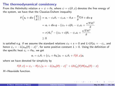
The thermodynamical consistencyFrom the Helmholtz relation e = ψ + θs where ψ = ψ(θ z) denotes the free energy ofthe system we have that the Clausius-Duhem inequality
θ(st + div
(qθ
))= et minus ψθθt minus ψzzt minus θts minus
q
θnablaθ + div q
= et + div q minus (ψθ + s)θt minus ψzzt +κ|nablaθ|2
θ
= σ|At |2 minus (ψθ + s)θt minus ψzzt +κ|nablaθ|2
θ
ge 0
is satisfied eg if we assume the standard relations ψθ + s = 0 and Lτ(θ)zt = minusψz andhence ψz = minusL(zeq(θ)minus z)+ for some positive constant L gt 0 Using the definition ofthe specific heat cv = θsθ we get
et = cvθt + (ψz + θsz)zt = cvθt + f (θ z)zt
where we have denoted for simplicity by
f (θ z) = ψz minus θ(ψz)θ = minusL(zeq(θ)minus z)+ + Lθz primeeq(θ)H(zeq(θ)minus z)
H=Heaviside function The internal energy balance results
cvθt + div q = σ|At |2 minus f (θ z)zt in Σtimes (0T )
E Rocca (Universita di Milano) Induction hardening May 14 2013 14 39
The PDE system
Model consists of vector-potential formulation ofMaxwellrsquos equation heat equation and rate law for phasefractions
Source term u can be used as control for optimization
σAt + curl1
microcurlA = J0u in D times (0T )
θt minus div κnablaθ = σ|At |2 + F(θ z)zt in Σtimes (0T )
zt =1
τ(θ)(zeq(θ)minus z)+ in Σtimes (0T )
where
J0 =(minusy(x2 + y 2) x(x2 + y 2) 0
)TF(θ z) = L(zeq(θ)minus θz primeeq(θ)minus z)
E Rocca (Universita di Milano) Induction hardening May 14 2013 15 39
Analysis and control of Joule heating models ndash a few references
Resistance heating
heat source h = σ|nablaϕ|2 minusrarr thermistor problem
Cimatti Prodi (1988) Howison Rodrigues Shillor (1993) Antonsev Chipot(1994) Homberg Khludnev Sokolowski (2001) Homberg Meyer Rehberg (2010)Homberg R (2011)
Induction heating ndash time domain
heat source h = σ(θ)|nablaϕ+ At |2
Bossavit Rodrigues (1994) Homberg Sokolowski (2003) optimal shape designHomberg (2004) including mechanical effects minusrarr the L1-regularity of the rhs inthe internal energy balance minusrarr weak solutions via Boccardo-Gallouet estimates
Induction heating ndash frequency domain
Bachinger Langer Schoberl Numerical analysis of nonlinear multiharmonic eddy currentproblems Numer Math 100 (2005)
Druet Klein Sprekels Troltzsch Yousept Optimal control of 3D state-constrainedinduction heating problems with nonlocal radiation effects SICON 49 (2011)
Troltzsch Yousept PDEndashconstrained optimization of time-dependent 3D electromagneticinduction heating by alternating voltages ESAIM M2AN 46 (2012)
E Rocca (Universita di Milano) Induction hardening May 14 2013 16 39
Analysis and control of Joule heating models ndash a few references
Resistance heating
heat source h = σ|nablaϕ|2 minusrarr thermistor problem
Cimatti Prodi (1988) Howison Rodrigues Shillor (1993) Antonsev Chipot(1994) Homberg Khludnev Sokolowski (2001) Homberg Meyer Rehberg (2010)Homberg R (2011)
Induction heating ndash time domain
heat source h = σ(θ)|nablaϕ+ At |2
Bossavit Rodrigues (1994) Homberg Sokolowski (2003) optimal shape designHomberg (2004) including mechanical effects minusrarr the L1-regularity of the rhs inthe internal energy balance minusrarr weak solutions via Boccardo-Gallouet estimates
Induction heating ndash frequency domain
Bachinger Langer Schoberl Numerical analysis of nonlinear multiharmonic eddy currentproblems Numer Math 100 (2005)
Druet Klein Sprekels Troltzsch Yousept Optimal control of 3D state-constrainedinduction heating problems with nonlocal radiation effects SICON 49 (2011)
Troltzsch Yousept PDEndashconstrained optimization of time-dependent 3D electromagneticinduction heating by alternating voltages ESAIM M2AN 46 (2012)
E Rocca (Universita di Milano) Induction hardening May 14 2013 16 39
Analysis and control of Joule heating models ndash a few references
Resistance heating
heat source h = σ|nablaϕ|2 minusrarr thermistor problem
Cimatti Prodi (1988) Howison Rodrigues Shillor (1993) Antonsev Chipot(1994) Homberg Khludnev Sokolowski (2001) Homberg Meyer Rehberg (2010)Homberg R (2011)
Induction heating ndash time domain
heat source h = σ(θ)|nablaϕ+ At |2
Bossavit Rodrigues (1994) Homberg Sokolowski (2003) optimal shape designHomberg (2004) including mechanical effects minusrarr the L1-regularity of the rhs inthe internal energy balance minusrarr weak solutions via Boccardo-Gallouet estimates
Induction heating ndash frequency domain
Bachinger Langer Schoberl Numerical analysis of nonlinear multiharmonic eddy currentproblems Numer Math 100 (2005)
Druet Klein Sprekels Troltzsch Yousept Optimal control of 3D state-constrainedinduction heating problems with nonlocal radiation effects SICON 49 (2011)
Troltzsch Yousept PDEndashconstrained optimization of time-dependent 3D electromagneticinduction heating by alternating voltages ESAIM M2AN 46 (2012)
E Rocca (Universita di Milano) Induction hardening May 14 2013 16 39
Analysis and control of Joule heating models ndash a few references
Resistance heating
heat source h = σ|nablaϕ|2 minusrarr thermistor problem
Cimatti Prodi (1988) Howison Rodrigues Shillor (1993) Antonsev Chipot(1994) Homberg Khludnev Sokolowski (2001) Homberg Meyer Rehberg (2010)Homberg R (2011)
Induction heating ndash time domain
heat source h = σ(θ)|nablaϕ+ At |2
Bossavit Rodrigues (1994) Homberg Sokolowski (2003) optimal shape designHomberg (2004) including mechanical effects minusrarr the L1-regularity of the rhs inthe internal energy balance minusrarr weak solutions via Boccardo-Gallouet estimates
Induction heating ndash frequency domain
Bachinger Langer Schoberl Numerical analysis of nonlinear multiharmonic eddy currentproblems Numer Math 100 (2005)
Druet Klein Sprekels Troltzsch Yousept Optimal control of 3D state-constrainedinduction heating problems with nonlocal radiation effects SICON 49 (2011)
Troltzsch Yousept PDEndashconstrained optimization of time-dependent 3D electromagneticinduction heating by alternating voltages ESAIM M2AN 46 (2012)
E Rocca (Universita di Milano) Induction hardening May 14 2013 16 39
Our results work in progess with D Hoemberg
Well-posedness of state system
Optimality conditions
E Rocca (Universita di Milano) Induction hardening May 14 2013 17 39
Our results work in progess with D Hoemberg
Well-posedness of state system
Optimality conditions
E Rocca (Universita di Milano) Induction hardening May 14 2013 17 39
Our results work in progess with D Hoemberg
Well-posedness of state system
Optimality conditions
E Rocca (Universita di Milano) Induction hardening May 14 2013 17 39
Solution space for vector potential
X =v isin L2(D)
∣∣∣ curl v isin L2(D) div v = 0 n times v∣∣∣partD
= 0
Assume partD isin C 11 Then X equipped with the norm
vX = curl vL2(D)
is a closed subspace of H1(D)
E Rocca (Universita di Milano) Induction hardening May 14 2013 18 39
Assumptions
(i) σ(x z) micro(x z) D times [0 1]rarr R are continuousand Lipschitz continuous (wrt z for almost allx isin D) function st
σ le σ(x z) le σ in D times [0 1]
micro le micro(x z) le micro in D times [0 1]
(ii) u isin H1(0T )
(iii) J0 D rarr R3 is an L2curl(D)-function
(iv) τ zeq isin C 2(R) and
τlowast le τ(θ) le τlowast 0 le zeq(θ) le 1
τC2(R) zeqC2(R) le M
| minus zeq(θ) + θz primeeq(θ)| |θz primeprimeeq(θ)| le M for all θ isin R
(v) g isin Linfin(0T Linfin(partΣ))
(vi) A0 isin X capH3(D) θ0 isinW 253(Σ)
E Rocca (Universita di Milano) Induction hardening May 14 2013 19 39
Weak formulation
Find a triple (A θ z) with the regularity properties
A isin H2(0T L2(D)) capW 1infin(0T X) curlA isin Linfin(0T L6(D)) (1)
θ isinW 153(0T L53(Σ)) cap L53(0T W 253(Σ)) cap L2(0T H1(Σ)) cap Linfin(Q) (2)
z isinW 1infin(0T W 1infin(Σ)) 0 le z lt 1 ae in Q (3)
solving the following systemintΩcupΣ
σ(x z)At middot v dx +
intD
1
micro(x z)curlA middot curl v dx =
intΩ
J0(x)u(t) middot v dx (4)
for all v isin X ae in (0T )
θt minus∆θ = minusF(θ z)zt + σ(x z)|At |2 ae in Q (5)
zt =1
τ(θ)(zeq(θ)minus z)+ ae in Q (6)
partθ
partν+ θ = g ae on partΣtimes (0T ) (7)
A(0) = A0 ae in D θ(0) = θ0 z(0) = 0 ae in Σ (8)
E Rocca (Universita di Milano) Induction hardening May 14 2013 20 39
Well-posedness result
Theorem 1 There exists a unique solution to (4)-(8) satisfying the regularities (1)-(3)and the following estimate
AH2(0T L2(D))capW 1infin(0T X) + curlALinfin(0T L6(D))
+ θW 153(0T L53(Σ))capL53(0T W 253(Σ))capL2(0T H1(Σ))capLinfin(Q) + zW 1infin(0T W 1infin(Σ)) le S
If we denote by (Ai θi zi ) (i = 1 2) two triples of solutions corresponding to data(A0i θ0i ui ) then there exists a positive constant C = C(S) such that the followingstability estimate holds true
(A1 minus A2)(t)2L2(D) + curl(A1 minus A2)2
L2(Dtimes(0T ))
+ partt(A1 minus A2)(t)2L2(D) + curl(partt(A1 minus A2))2
L2(Dtimes(0T ))
+ (θ1 minus θ2)(t)2L2(Σ) + θ1 minus θ22
L2(0T H1(Σ))
+ (z1 minus z2)(t)2H1(Σ) + partt(z1 minus z2)2
L2(0T H1(Σ))
le C(A01 minus A022
X + (partt(A1 minus A2))(0)2L2(D) + θ01 minus θ022
L2(Σ)
+u1J0 minus u2J02L2(0T ) + uprime1J0 minus uprime2J02
L2(0T )
)for all t isin [0T ]
E Rocca (Universita di Milano) Induction hardening May 14 2013 21 39
Well-posedness result
Theorem 1 There exists a unique solution to (4)-(8) satisfying the regularities (1)-(3)and the following estimate
AH2(0T L2(D))capW 1infin(0T X) + curlALinfin(0T L6(D))
+ θW 153(0T L53(Σ))capL53(0T W 253(Σ))capL2(0T H1(Σ))capLinfin(Q) + zW 1infin(0T W 1infin(Σ)) le S
If we denote by (Ai θi zi ) (i = 1 2) two triples of solutions corresponding to data(A0i θ0i ui ) then there exists a positive constant C = C(S) such that the followingstability estimate holds true
(A1 minus A2)(t)2L2(D) + curl(A1 minus A2)2
L2(Dtimes(0T ))
+ partt(A1 minus A2)(t)2L2(D) + curl(partt(A1 minus A2))2
L2(Dtimes(0T ))
+ (θ1 minus θ2)(t)2L2(Σ) + θ1 minus θ22
L2(0T H1(Σ))
+ (z1 minus z2)(t)2H1(Σ) + partt(z1 minus z2)2
L2(0T H1(Σ))
le C(A01 minus A022
X + (partt(A1 minus A2))(0)2L2(D) + θ01 minus θ022
L2(Σ)
+u1J0 minus u2J02L2(0T ) + uprime1J0 minus uprime2J02
L2(0T )
)for all t isin [0T ]
E Rocca (Universita di Milano) Induction hardening May 14 2013 21 39
Idea of the proof of Thm 1
Local existence via Shauder fixed point argument exploiting the Lipschitz continuityof the map θ 7rarr z from W 1p(0T0 Lp(Σ)) in itself
Global a-priori estimates on solutions1 Exploit the regularity and boundedness of the solution z to the ODE getting
zW 1infin(0T0Linfin(Σ)) le C 0 le z(x t) lt 1 ae in Q
2 Take first v = At then differentiate it (formally) in time and take v = At inintΩcupΣ
σ(x z)At middot v dx +
intD
1
micro(x z)curlA middot curl v dx =
intΩJ0(x)u(t) middot v dx
and use Est 1 and the assumptions on micro and σ getting
AH1(0T0X)capW 1infin(0T0L2(D)) + AtL103(Dtimes(0T0)) le C
3 Testθt minus∆θ = minusF(θ z)zt + σ(x z)|At |2
by θ and using maximal regularity results for parabolic equations we get
θL2(0T0H1(Σ))capLinfin(0T0L2(Σ))capL53(0T0W 253(Σ))capW 153(0T0L53(Σ)) le C
4 Differentiating (formally) the A-eq and taking v = Att arguing by comparison andusing the results of [Kawanago rsquo93] in order to prove the Linfin-estimate for θ we getthe desired regularity of solutions and we can prolpongate it over the whole timeinterval [0T ]
E Rocca (Universita di Milano) Induction hardening May 14 2013 22 39
Idea of the proof of Thm 1
Local existence via Shauder fixed point argument exploiting the Lipschitz continuityof the map θ 7rarr z from W 1p(0T0 Lp(Σ)) in itself
Global a-priori estimates on solutions1 Exploit the regularity and boundedness of the solution z to the ODE getting
zW 1infin(0T0Linfin(Σ)) le C 0 le z(x t) lt 1 ae in Q
2 Take first v = At then differentiate it (formally) in time and take v = At inintΩcupΣ
σ(x z)At middot v dx +
intD
1
micro(x z)curlA middot curl v dx =
intΩJ0(x)u(t) middot v dx
and use Est 1 and the assumptions on micro and σ getting
AH1(0T0X)capW 1infin(0T0L2(D)) + AtL103(Dtimes(0T0)) le C
3 Testθt minus∆θ = minusF(θ z)zt + σ(x z)|At |2
by θ and using maximal regularity results for parabolic equations we get
θL2(0T0H1(Σ))capLinfin(0T0L2(Σ))capL53(0T0W 253(Σ))capW 153(0T0L53(Σ)) le C
4 Differentiating (formally) the A-eq and taking v = Att arguing by comparison andusing the results of [Kawanago rsquo93] in order to prove the Linfin-estimate for θ we getthe desired regularity of solutions and we can prolpongate it over the whole timeinterval [0T ]
E Rocca (Universita di Milano) Induction hardening May 14 2013 22 39
Idea of the proof of Thm 1
Local existence via Shauder fixed point argument exploiting the Lipschitz continuityof the map θ 7rarr z from W 1p(0T0 Lp(Σ)) in itself
Global a-priori estimates on solutions1 Exploit the regularity and boundedness of the solution z to the ODE getting
zW 1infin(0T0Linfin(Σ)) le C 0 le z(x t) lt 1 ae in Q
2 Take first v = At then differentiate it (formally) in time and take v = At inintΩcupΣ
σ(x z)At middot v dx +
intD
1
micro(x z)curlA middot curl v dx =
intΩJ0(x)u(t) middot v dx
and use Est 1 and the assumptions on micro and σ getting
AH1(0T0X)capW 1infin(0T0L2(D)) + AtL103(Dtimes(0T0)) le C
3 Testθt minus∆θ = minusF(θ z)zt + σ(x z)|At |2
by θ and using maximal regularity results for parabolic equations we get
θL2(0T0H1(Σ))capLinfin(0T0L2(Σ))capL53(0T0W 253(Σ))capW 153(0T0L53(Σ)) le C
4 Differentiating (formally) the A-eq and taking v = Att arguing by comparison andusing the results of [Kawanago rsquo93] in order to prove the Linfin-estimate for θ we getthe desired regularity of solutions and we can prolpongate it over the whole timeinterval [0T ]
E Rocca (Universita di Milano) Induction hardening May 14 2013 22 39
Idea of the proof of Thm 1
Local existence via Shauder fixed point argument exploiting the Lipschitz continuityof the map θ 7rarr z from W 1p(0T0 Lp(Σ)) in itself
Global a-priori estimates on solutions1 Exploit the regularity and boundedness of the solution z to the ODE getting
zW 1infin(0T0Linfin(Σ)) le C 0 le z(x t) lt 1 ae in Q
2 Take first v = At then differentiate it (formally) in time and take v = At inintΩcupΣ
σ(x z)At middot v dx +
intD
1
micro(x z)curlA middot curl v dx =
intΩJ0(x)u(t) middot v dx
and use Est 1 and the assumptions on micro and σ getting
AH1(0T0X)capW 1infin(0T0L2(D)) + AtL103(Dtimes(0T0)) le C
3 Testθt minus∆θ = minusF(θ z)zt + σ(x z)|At |2
by θ and using maximal regularity results for parabolic equations we get
θL2(0T0H1(Σ))capLinfin(0T0L2(Σ))capL53(0T0W 253(Σ))capW 153(0T0L53(Σ)) le C
4 Differentiating (formally) the A-eq and taking v = Att arguing by comparison andusing the results of [Kawanago rsquo93] in order to prove the Linfin-estimate for θ we getthe desired regularity of solutions and we can prolpongate it over the whole timeinterval [0T ]
E Rocca (Universita di Milano) Induction hardening May 14 2013 22 39
Idea of the proof of Thm 1
Local existence via Shauder fixed point argument exploiting the Lipschitz continuityof the map θ 7rarr z from W 1p(0T0 Lp(Σ)) in itself
Global a-priori estimates on solutions1 Exploit the regularity and boundedness of the solution z to the ODE getting
zW 1infin(0T0Linfin(Σ)) le C 0 le z(x t) lt 1 ae in Q
2 Take first v = At then differentiate it (formally) in time and take v = At inintΩcupΣ
σ(x z)At middot v dx +
intD
1
micro(x z)curlA middot curl v dx =
intΩJ0(x)u(t) middot v dx
and use Est 1 and the assumptions on micro and σ getting
AH1(0T0X)capW 1infin(0T0L2(D)) + AtL103(Dtimes(0T0)) le C
3 Testθt minus∆θ = minusF(θ z)zt + σ(x z)|At |2
by θ and using maximal regularity results for parabolic equations we get
θL2(0T0H1(Σ))capLinfin(0T0L2(Σ))capL53(0T0W 253(Σ))capW 153(0T0L53(Σ)) le C
4 Differentiating (formally) the A-eq and taking v = Att arguing by comparison andusing the results of [Kawanago rsquo93] in order to prove the Linfin-estimate for θ we getthe desired regularity of solutions and we can prolpongate it over the whole timeinterval [0T ]
E Rocca (Universita di Milano) Induction hardening May 14 2013 22 39
Stability estimate
Differentiate in time equationintΩcupΣ
σ(x z)At middot v dx +
intD
1
micro(x z)curlA middot curl v dx =
intΩ
J0(x)u(t) middot v dx
and take the difference of the two differentiated relations in two solutions (Ai θi zi )and test the difference by (A1 minus A2)t
Use the Lipschitz continuity properties of the solution map to the ODE in z
Take the differences of the equations for θ and test by θ1 minus θ2 exploit the regularityof A and sum up the two relations
E Rocca (Universita di Milano) Induction hardening May 14 2013 23 39
Optimal control problem ndash Existence
cost functional
J (A θ z u) =β1
2
Tint0
intΣ
(θ(x t)minus θd(x t))2dxdt +
β2
2
intΣ
(z(x T )minus zd)2dx +β3
2u2
H1(0T )
control problem (CP)minJ (A θ z u)such that A θ z satisfies (P) and u isin Uad sub H1(0T )
Theorem 2 (CP) has a solution u isin Uad
E Rocca (Universita di Milano) Induction hardening May 14 2013 24 39
Optimal control problem ndash Existence
cost functional
J (A θ z u) =β1
2
Tint0
intΣ
(θ(x t)minus θd(x t))2dxdt +
β2
2
intΣ
(z(x T )minus zd)2dx +β3
2u2
H1(0T )
control problem (CP)minJ (A θ z u)such that A θ z satisfies (P) and u isin Uad sub H1(0T )
Theorem 2 (CP) has a solution u isin Uad
E Rocca (Universita di Milano) Induction hardening May 14 2013 24 39
Optimal control problem ndash Existence
cost functional
J (A θ z u) =β1
2
Tint0
intΣ
(θ(x t)minus θd(x t))2dxdt +
β2
2
intΣ
(z(x T )minus zd)2dx +β3
2u2
H1(0T )
control problem (CP)minJ (A θ z u)such that A θ z satisfies (P) and u isin Uad sub H1(0T )
Theorem 2 (CP) has a solution u isin Uad
E Rocca (Universita di Milano) Induction hardening May 14 2013 24 39
Optimal control problem ndash Differentiability
Lipschitz-continuity the control-to-state mapping
S u 7rarr (A θ z)
is Lipschitz continuous from H1(0T ) to Z by Theorem 1
Frechet differentiability the control-to-state mapping
S u 7rarr (A θ z)
is Frechet differentiable from H1(0T ) to Y Z sub Y
E Rocca (Universita di Milano) Induction hardening May 14 2013 25 39
Optimal control problem ndash First-order necessary conditions of optimality
adjoint systemminusσαt minus curl
( 1
microcurlα
)minus σprime(x z)ztα = minus2(σAtϑ)t
minusϑt minus k∆ϑ+ fθ(θ z)ϑ = fθζ + β1(θ minus θd)
minusζt minus fz(θ z)ζ + σprimeAt middotαminus σprime|At |2ϑ =microprime
micro2curlA middot curlαminus fzϑ
αtimes n = 0 in partD times (0T )
kpartϑ
partν+ κϑ = 0 in partΣtimes (0T )
ϑ(T ) = 0 ζ(T ) = z(x T )minus zd(x) in Σ
α(T ) = 0 in D
variational inequalityTint
0
(β3u(t)minus
intD
α(x t) middot J0(x t)dx)
(u minus u)dt
+
Tint0
β3uprime(t)(uprime(t)minus uprime(t))dt ge 0 for all u isin Uad sub H1(0T )
E Rocca (Universita di Milano) Induction hardening May 14 2013 26 39
Optimal control problem ndash First-order necessary conditions of optimality
adjoint systemminusσαt minus curl
( 1
microcurlα
)minus σprime(x z)ztα = minus2(σAtϑ)t
minusϑt minus k∆ϑ+ fθ(θ z)ϑ = fθζ + β1(θ minus θd)
minusζt minus fz(θ z)ζ + σprimeAt middotαminus σprime|At |2ϑ =microprime
micro2curlA middot curlαminus fzϑ
αtimes n = 0 in partD times (0T )
kpartϑ
partν+ κϑ = 0 in partΣtimes (0T )
ϑ(T ) = 0 ζ(T ) = z(x T )minus zd(x) in Σ
α(T ) = 0 in D
variational inequalityTint
0
(β3u(t)minus
intD
α(x t) middot J0(x t)dx)
(u minus u)dt
+
Tint0
β3uprime(t)(uprime(t)minus uprime(t))dt ge 0 for all u isin Uad sub H1(0T )
E Rocca (Universita di Milano) Induction hardening May 14 2013 26 39
Numerical results ndash Challenges [Homberg Petzold]
Multiple time scalesMagnetic vector potential and heat conductance live on different time scales(Averaging method)
Skin effectEddy currents are distributed in a small surface layer of the workpiece (Adaptivemesh generation)
Nonlinear material dataMagnetic permeability micro depends on temperature and magnetic field H(Linearization)
3DTime consuming simulation in 3D (Model reduction to tackle optimal controlproblem numerically)
E Rocca (Universita di Milano) Induction hardening May 14 2013 27 39
Numerical results ndash Challenges [Homberg Petzold]
Multiple time scalesMagnetic vector potential and heat conductance live on different time scales(Averaging method)
Skin effectEddy currents are distributed in a small surface layer of the workpiece (Adaptivemesh generation)
Nonlinear material dataMagnetic permeability micro depends on temperature and magnetic field H(Linearization)
3DTime consuming simulation in 3D (Model reduction to tackle optimal controlproblem numerically)
E Rocca (Universita di Milano) Induction hardening May 14 2013 27 39
Numerical results ndash Challenges [Homberg Petzold]
Multiple time scalesMagnetic vector potential and heat conductance live on different time scales(Averaging method)
Skin effectEddy currents are distributed in a small surface layer of the workpiece (Adaptivemesh generation)
Nonlinear material dataMagnetic permeability micro depends on temperature and magnetic field H(Linearization)
3DTime consuming simulation in 3D (Model reduction to tackle optimal controlproblem numerically)
E Rocca (Universita di Milano) Induction hardening May 14 2013 27 39
Numerical results ndash Challenges [Homberg Petzold]
Multiple time scalesMagnetic vector potential and heat conductance live on different time scales(Averaging method)
Skin effectEddy currents are distributed in a small surface layer of the workpiece (Adaptivemesh generation)
Nonlinear material dataMagnetic permeability micro depends on temperature and magnetic field H(Linearization)
3DTime consuming simulation in 3D (Model reduction to tackle optimal controlproblem numerically)
E Rocca (Universita di Milano) Induction hardening May 14 2013 27 39
Numerical realization ndash multiple time scales
Time scale for Maxwellrsquos equation governed by frequency of source currentf asymp 10 kHzminus 100 kHz consequetly τ sim 10minus5s
Time scale for heat equation governed by heat diffusion
τ sim cpρL2
kasymp 1 s
Alternating computation
I Solve for A with fixed temperature on fast time-scale
I Compute Joule heat by averaging electric energy Q = 1T
int T0 σ
∣∣∣ partApartt ∣∣∣2 dt
I Solve heat equation with fixed magnetic potential on slow time-scale (one time step)I Update A since σ and micro change with temperature
E Rocca (Universita di Milano) Induction hardening May 14 2013 28 39
Numerical realization ndash multiple time scales
Time scale for Maxwellrsquos equation governed by frequency of source currentf asymp 10 kHzminus 100 kHz consequetly τ sim 10minus5s
Time scale for heat equation governed by heat diffusion
τ sim cpρL2
kasymp 1 s
Alternating computation
I Solve for A with fixed temperature on fast time-scale
I Compute Joule heat by averaging electric energy Q = 1T
int T0 σ
∣∣∣ partApartt ∣∣∣2 dt
I Solve heat equation with fixed magnetic potential on slow time-scale (one time step)I Update A since σ and micro change with temperature
E Rocca (Universita di Milano) Induction hardening May 14 2013 28 39
Thermal and electrical conductivity heat capacity and density
Material data depend on temperature
Electrical conductivity σ(θ)Thermal conductivity κ(θ)
Density ρ(θ)Specific heat capacity cp(θ)
Nonlinear relation between magnetic induction B and magnetic field HMagnetization curve B = micro(θH)H
E Rocca (Universita di Milano) Induction hardening May 14 2013 29 39
Example 1 HF temperature and growth of austenite
(Video austenitemp4)
Figure temperature and austenite growth at high frequency
E Rocca (Universita di Milano) Induction hardening May 14 2013 30 39

Analysis and control of Joule heating models ndash a few references
Resistance heating
heat source h = σ|nablaϕ|2 minusrarr thermistor problem
Cimatti Prodi (1988) Howison Rodrigues Shillor (1993) Antonsev Chipot(1994) Homberg Khludnev Sokolowski (2001) Homberg Meyer Rehberg (2010)Homberg R (2011)
Induction heating ndash time domain
heat source h = σ(θ)|nablaϕ+ At |2
Bossavit Rodrigues (1994) Homberg Sokolowski (2003) optimal shape designHomberg (2004) including mechanical effects minusrarr the L1-regularity of the rhs inthe internal energy balance minusrarr weak solutions via Boccardo-Gallouet estimates
Induction heating ndash frequency domain
Bachinger Langer Schoberl Numerical analysis of nonlinear multiharmonic eddy currentproblems Numer Math 100 (2005)
Druet Klein Sprekels Troltzsch Yousept Optimal control of 3D state-constrainedinduction heating problems with nonlocal radiation effects SICON 49 (2011)
Troltzsch Yousept PDEndashconstrained optimization of time-dependent 3D electromagneticinduction heating by alternating voltages ESAIM M2AN 46 (2012)
E Rocca (Universita di Milano) Induction hardening May 14 2013 16 39
Our results work in progess with D Hoemberg
Well-posedness of state system
Optimality conditions
E Rocca (Universita di Milano) Induction hardening May 14 2013 17 39
Our results work in progess with D Hoemberg
Well-posedness of state system
Optimality conditions
E Rocca (Universita di Milano) Induction hardening May 14 2013 17 39
Our results work in progess with D Hoemberg
Well-posedness of state system
Optimality conditions
E Rocca (Universita di Milano) Induction hardening May 14 2013 17 39
Solution space for vector potential
X =v isin L2(D)
∣∣∣ curl v isin L2(D) div v = 0 n times v∣∣∣partD
= 0
Assume partD isin C 11 Then X equipped with the norm
vX = curl vL2(D)
is a closed subspace of H1(D)
E Rocca (Universita di Milano) Induction hardening May 14 2013 18 39
Assumptions
(i) σ(x z) micro(x z) D times [0 1]rarr R are continuousand Lipschitz continuous (wrt z for almost allx isin D) function st
σ le σ(x z) le σ in D times [0 1]
micro le micro(x z) le micro in D times [0 1]
(ii) u isin H1(0T )
(iii) J0 D rarr R3 is an L2curl(D)-function
(iv) τ zeq isin C 2(R) and
τlowast le τ(θ) le τlowast 0 le zeq(θ) le 1
τC2(R) zeqC2(R) le M
| minus zeq(θ) + θz primeeq(θ)| |θz primeprimeeq(θ)| le M for all θ isin R
(v) g isin Linfin(0T Linfin(partΣ))
(vi) A0 isin X capH3(D) θ0 isinW 253(Σ)
E Rocca (Universita di Milano) Induction hardening May 14 2013 19 39
Weak formulation
Find a triple (A θ z) with the regularity properties
A isin H2(0T L2(D)) capW 1infin(0T X) curlA isin Linfin(0T L6(D)) (1)
θ isinW 153(0T L53(Σ)) cap L53(0T W 253(Σ)) cap L2(0T H1(Σ)) cap Linfin(Q) (2)
z isinW 1infin(0T W 1infin(Σ)) 0 le z lt 1 ae in Q (3)
solving the following systemintΩcupΣ
σ(x z)At middot v dx +
intD
1
micro(x z)curlA middot curl v dx =
intΩ
J0(x)u(t) middot v dx (4)
for all v isin X ae in (0T )
θt minus∆θ = minusF(θ z)zt + σ(x z)|At |2 ae in Q (5)
zt =1
τ(θ)(zeq(θ)minus z)+ ae in Q (6)
partθ
partν+ θ = g ae on partΣtimes (0T ) (7)
A(0) = A0 ae in D θ(0) = θ0 z(0) = 0 ae in Σ (8)
E Rocca (Universita di Milano) Induction hardening May 14 2013 20 39
Well-posedness result
Theorem 1 There exists a unique solution to (4)-(8) satisfying the regularities (1)-(3)and the following estimate
AH2(0T L2(D))capW 1infin(0T X) + curlALinfin(0T L6(D))
+ θW 153(0T L53(Σ))capL53(0T W 253(Σ))capL2(0T H1(Σ))capLinfin(Q) + zW 1infin(0T W 1infin(Σ)) le S
If we denote by (Ai θi zi ) (i = 1 2) two triples of solutions corresponding to data(A0i θ0i ui ) then there exists a positive constant C = C(S) such that the followingstability estimate holds true
(A1 minus A2)(t)2L2(D) + curl(A1 minus A2)2
L2(Dtimes(0T ))
+ partt(A1 minus A2)(t)2L2(D) + curl(partt(A1 minus A2))2
L2(Dtimes(0T ))
+ (θ1 minus θ2)(t)2L2(Σ) + θ1 minus θ22
L2(0T H1(Σ))
+ (z1 minus z2)(t)2H1(Σ) + partt(z1 minus z2)2
L2(0T H1(Σ))
le C(A01 minus A022
X + (partt(A1 minus A2))(0)2L2(D) + θ01 minus θ022
L2(Σ)
+u1J0 minus u2J02L2(0T ) + uprime1J0 minus uprime2J02
L2(0T )
)for all t isin [0T ]
E Rocca (Universita di Milano) Induction hardening May 14 2013 21 39
Well-posedness result
Theorem 1 There exists a unique solution to (4)-(8) satisfying the regularities (1)-(3)and the following estimate
AH2(0T L2(D))capW 1infin(0T X) + curlALinfin(0T L6(D))
+ θW 153(0T L53(Σ))capL53(0T W 253(Σ))capL2(0T H1(Σ))capLinfin(Q) + zW 1infin(0T W 1infin(Σ)) le S
If we denote by (Ai θi zi ) (i = 1 2) two triples of solutions corresponding to data(A0i θ0i ui ) then there exists a positive constant C = C(S) such that the followingstability estimate holds true
(A1 minus A2)(t)2L2(D) + curl(A1 minus A2)2
L2(Dtimes(0T ))
+ partt(A1 minus A2)(t)2L2(D) + curl(partt(A1 minus A2))2
L2(Dtimes(0T ))
+ (θ1 minus θ2)(t)2L2(Σ) + θ1 minus θ22
L2(0T H1(Σ))
+ (z1 minus z2)(t)2H1(Σ) + partt(z1 minus z2)2
L2(0T H1(Σ))
le C(A01 minus A022
X + (partt(A1 minus A2))(0)2L2(D) + θ01 minus θ022
L2(Σ)
+u1J0 minus u2J02L2(0T ) + uprime1J0 minus uprime2J02
L2(0T )
)for all t isin [0T ]
E Rocca (Universita di Milano) Induction hardening May 14 2013 21 39
Idea of the proof of Thm 1
Local existence via Shauder fixed point argument exploiting the Lipschitz continuityof the map θ 7rarr z from W 1p(0T0 Lp(Σ)) in itself
Global a-priori estimates on solutions1 Exploit the regularity and boundedness of the solution z to the ODE getting
zW 1infin(0T0Linfin(Σ)) le C 0 le z(x t) lt 1 ae in Q
2 Take first v = At then differentiate it (formally) in time and take v = At inintΩcupΣ
σ(x z)At middot v dx +
intD
1
micro(x z)curlA middot curl v dx =
intΩJ0(x)u(t) middot v dx
and use Est 1 and the assumptions on micro and σ getting
AH1(0T0X)capW 1infin(0T0L2(D)) + AtL103(Dtimes(0T0)) le C
3 Testθt minus∆θ = minusF(θ z)zt + σ(x z)|At |2
by θ and using maximal regularity results for parabolic equations we get
θL2(0T0H1(Σ))capLinfin(0T0L2(Σ))capL53(0T0W 253(Σ))capW 153(0T0L53(Σ)) le C
4 Differentiating (formally) the A-eq and taking v = Att arguing by comparison andusing the results of [Kawanago rsquo93] in order to prove the Linfin-estimate for θ we getthe desired regularity of solutions and we can prolpongate it over the whole timeinterval [0T ]
E Rocca (Universita di Milano) Induction hardening May 14 2013 22 39
Idea of the proof of Thm 1
Local existence via Shauder fixed point argument exploiting the Lipschitz continuityof the map θ 7rarr z from W 1p(0T0 Lp(Σ)) in itself
Global a-priori estimates on solutions1 Exploit the regularity and boundedness of the solution z to the ODE getting
zW 1infin(0T0Linfin(Σ)) le C 0 le z(x t) lt 1 ae in Q
2 Take first v = At then differentiate it (formally) in time and take v = At inintΩcupΣ
σ(x z)At middot v dx +
intD
1
micro(x z)curlA middot curl v dx =
intΩJ0(x)u(t) middot v dx
and use Est 1 and the assumptions on micro and σ getting
AH1(0T0X)capW 1infin(0T0L2(D)) + AtL103(Dtimes(0T0)) le C
3 Testθt minus∆θ = minusF(θ z)zt + σ(x z)|At |2
by θ and using maximal regularity results for parabolic equations we get
θL2(0T0H1(Σ))capLinfin(0T0L2(Σ))capL53(0T0W 253(Σ))capW 153(0T0L53(Σ)) le C
4 Differentiating (formally) the A-eq and taking v = Att arguing by comparison andusing the results of [Kawanago rsquo93] in order to prove the Linfin-estimate for θ we getthe desired regularity of solutions and we can prolpongate it over the whole timeinterval [0T ]
E Rocca (Universita di Milano) Induction hardening May 14 2013 22 39
Idea of the proof of Thm 1
Local existence via Shauder fixed point argument exploiting the Lipschitz continuityof the map θ 7rarr z from W 1p(0T0 Lp(Σ)) in itself
Global a-priori estimates on solutions1 Exploit the regularity and boundedness of the solution z to the ODE getting
zW 1infin(0T0Linfin(Σ)) le C 0 le z(x t) lt 1 ae in Q
2 Take first v = At then differentiate it (formally) in time and take v = At inintΩcupΣ
σ(x z)At middot v dx +
intD
1
micro(x z)curlA middot curl v dx =
intΩJ0(x)u(t) middot v dx
and use Est 1 and the assumptions on micro and σ getting
AH1(0T0X)capW 1infin(0T0L2(D)) + AtL103(Dtimes(0T0)) le C
3 Testθt minus∆θ = minusF(θ z)zt + σ(x z)|At |2
by θ and using maximal regularity results for parabolic equations we get
θL2(0T0H1(Σ))capLinfin(0T0L2(Σ))capL53(0T0W 253(Σ))capW 153(0T0L53(Σ)) le C
4 Differentiating (formally) the A-eq and taking v = Att arguing by comparison andusing the results of [Kawanago rsquo93] in order to prove the Linfin-estimate for θ we getthe desired regularity of solutions and we can prolpongate it over the whole timeinterval [0T ]
E Rocca (Universita di Milano) Induction hardening May 14 2013 22 39
Idea of the proof of Thm 1
Local existence via Shauder fixed point argument exploiting the Lipschitz continuityof the map θ 7rarr z from W 1p(0T0 Lp(Σ)) in itself
Global a-priori estimates on solutions1 Exploit the regularity and boundedness of the solution z to the ODE getting
zW 1infin(0T0Linfin(Σ)) le C 0 le z(x t) lt 1 ae in Q
2 Take first v = At then differentiate it (formally) in time and take v = At inintΩcupΣ
σ(x z)At middot v dx +
intD
1
micro(x z)curlA middot curl v dx =
intΩJ0(x)u(t) middot v dx
and use Est 1 and the assumptions on micro and σ getting
AH1(0T0X)capW 1infin(0T0L2(D)) + AtL103(Dtimes(0T0)) le C
3 Testθt minus∆θ = minusF(θ z)zt + σ(x z)|At |2
by θ and using maximal regularity results for parabolic equations we get
θL2(0T0H1(Σ))capLinfin(0T0L2(Σ))capL53(0T0W 253(Σ))capW 153(0T0L53(Σ)) le C
4 Differentiating (formally) the A-eq and taking v = Att arguing by comparison andusing the results of [Kawanago rsquo93] in order to prove the Linfin-estimate for θ we getthe desired regularity of solutions and we can prolpongate it over the whole timeinterval [0T ]
E Rocca (Universita di Milano) Induction hardening May 14 2013 22 39
Idea of the proof of Thm 1
Local existence via Shauder fixed point argument exploiting the Lipschitz continuityof the map θ 7rarr z from W 1p(0T0 Lp(Σ)) in itself
Global a-priori estimates on solutions1 Exploit the regularity and boundedness of the solution z to the ODE getting
zW 1infin(0T0Linfin(Σ)) le C 0 le z(x t) lt 1 ae in Q
2 Take first v = At then differentiate it (formally) in time and take v = At inintΩcupΣ
σ(x z)At middot v dx +
intD
1
micro(x z)curlA middot curl v dx =
intΩJ0(x)u(t) middot v dx
and use Est 1 and the assumptions on micro and σ getting
AH1(0T0X)capW 1infin(0T0L2(D)) + AtL103(Dtimes(0T0)) le C
3 Testθt minus∆θ = minusF(θ z)zt + σ(x z)|At |2
by θ and using maximal regularity results for parabolic equations we get
θL2(0T0H1(Σ))capLinfin(0T0L2(Σ))capL53(0T0W 253(Σ))capW 153(0T0L53(Σ)) le C
4 Differentiating (formally) the A-eq and taking v = Att arguing by comparison andusing the results of [Kawanago rsquo93] in order to prove the Linfin-estimate for θ we getthe desired regularity of solutions and we can prolpongate it over the whole timeinterval [0T ]
E Rocca (Universita di Milano) Induction hardening May 14 2013 22 39
Stability estimate
Differentiate in time equationintΩcupΣ
σ(x z)At middot v dx +
intD
1
micro(x z)curlA middot curl v dx =
intΩ
J0(x)u(t) middot v dx
and take the difference of the two differentiated relations in two solutions (Ai θi zi )and test the difference by (A1 minus A2)t
Use the Lipschitz continuity properties of the solution map to the ODE in z
Take the differences of the equations for θ and test by θ1 minus θ2 exploit the regularityof A and sum up the two relations
E Rocca (Universita di Milano) Induction hardening May 14 2013 23 39
Optimal control problem ndash Existence
cost functional
J (A θ z u) =β1
2
Tint0
intΣ
(θ(x t)minus θd(x t))2dxdt +
β2
2
intΣ
(z(x T )minus zd)2dx +β3
2u2
H1(0T )
control problem (CP)minJ (A θ z u)such that A θ z satisfies (P) and u isin Uad sub H1(0T )
Theorem 2 (CP) has a solution u isin Uad
E Rocca (Universita di Milano) Induction hardening May 14 2013 24 39
Optimal control problem ndash Existence
cost functional
J (A θ z u) =β1
2
Tint0
intΣ
(θ(x t)minus θd(x t))2dxdt +
β2
2
intΣ
(z(x T )minus zd)2dx +β3
2u2
H1(0T )
control problem (CP)minJ (A θ z u)such that A θ z satisfies (P) and u isin Uad sub H1(0T )
Theorem 2 (CP) has a solution u isin Uad
E Rocca (Universita di Milano) Induction hardening May 14 2013 24 39
Optimal control problem ndash Existence
cost functional
J (A θ z u) =β1
2
Tint0
intΣ
(θ(x t)minus θd(x t))2dxdt +
β2
2
intΣ
(z(x T )minus zd)2dx +β3
2u2
H1(0T )
control problem (CP)minJ (A θ z u)such that A θ z satisfies (P) and u isin Uad sub H1(0T )
Theorem 2 (CP) has a solution u isin Uad
E Rocca (Universita di Milano) Induction hardening May 14 2013 24 39
Optimal control problem ndash Differentiability
Lipschitz-continuity the control-to-state mapping
S u 7rarr (A θ z)
is Lipschitz continuous from H1(0T ) to Z by Theorem 1
Frechet differentiability the control-to-state mapping
S u 7rarr (A θ z)
is Frechet differentiable from H1(0T ) to Y Z sub Y
E Rocca (Universita di Milano) Induction hardening May 14 2013 25 39
Optimal control problem ndash First-order necessary conditions of optimality
adjoint systemminusσαt minus curl
( 1
microcurlα
)minus σprime(x z)ztα = minus2(σAtϑ)t
minusϑt minus k∆ϑ+ fθ(θ z)ϑ = fθζ + β1(θ minus θd)
minusζt minus fz(θ z)ζ + σprimeAt middotαminus σprime|At |2ϑ =microprime
micro2curlA middot curlαminus fzϑ
αtimes n = 0 in partD times (0T )
kpartϑ
partν+ κϑ = 0 in partΣtimes (0T )
ϑ(T ) = 0 ζ(T ) = z(x T )minus zd(x) in Σ
α(T ) = 0 in D
variational inequalityTint
0
(β3u(t)minus
intD
α(x t) middot J0(x t)dx)
(u minus u)dt
+
Tint0
β3uprime(t)(uprime(t)minus uprime(t))dt ge 0 for all u isin Uad sub H1(0T )
E Rocca (Universita di Milano) Induction hardening May 14 2013 26 39
Optimal control problem ndash First-order necessary conditions of optimality
adjoint systemminusσαt minus curl
( 1
microcurlα
)minus σprime(x z)ztα = minus2(σAtϑ)t
minusϑt minus k∆ϑ+ fθ(θ z)ϑ = fθζ + β1(θ minus θd)
minusζt minus fz(θ z)ζ + σprimeAt middotαminus σprime|At |2ϑ =microprime
micro2curlA middot curlαminus fzϑ
αtimes n = 0 in partD times (0T )
kpartϑ
partν+ κϑ = 0 in partΣtimes (0T )
ϑ(T ) = 0 ζ(T ) = z(x T )minus zd(x) in Σ
α(T ) = 0 in D
variational inequalityTint
0
(β3u(t)minus
intD
α(x t) middot J0(x t)dx)
(u minus u)dt
+
Tint0
β3uprime(t)(uprime(t)minus uprime(t))dt ge 0 for all u isin Uad sub H1(0T )
E Rocca (Universita di Milano) Induction hardening May 14 2013 26 39
Numerical results ndash Challenges [Homberg Petzold]
Multiple time scalesMagnetic vector potential and heat conductance live on different time scales(Averaging method)
Skin effectEddy currents are distributed in a small surface layer of the workpiece (Adaptivemesh generation)
Nonlinear material dataMagnetic permeability micro depends on temperature and magnetic field H(Linearization)
3DTime consuming simulation in 3D (Model reduction to tackle optimal controlproblem numerically)
E Rocca (Universita di Milano) Induction hardening May 14 2013 27 39
Numerical results ndash Challenges [Homberg Petzold]
Multiple time scalesMagnetic vector potential and heat conductance live on different time scales(Averaging method)
Skin effectEddy currents are distributed in a small surface layer of the workpiece (Adaptivemesh generation)
Nonlinear material dataMagnetic permeability micro depends on temperature and magnetic field H(Linearization)
3DTime consuming simulation in 3D (Model reduction to tackle optimal controlproblem numerically)
E Rocca (Universita di Milano) Induction hardening May 14 2013 27 39
Numerical results ndash Challenges [Homberg Petzold]
Multiple time scalesMagnetic vector potential and heat conductance live on different time scales(Averaging method)
Skin effectEddy currents are distributed in a small surface layer of the workpiece (Adaptivemesh generation)
Nonlinear material dataMagnetic permeability micro depends on temperature and magnetic field H(Linearization)
3DTime consuming simulation in 3D (Model reduction to tackle optimal controlproblem numerically)
E Rocca (Universita di Milano) Induction hardening May 14 2013 27 39
Numerical results ndash Challenges [Homberg Petzold]
Multiple time scalesMagnetic vector potential and heat conductance live on different time scales(Averaging method)
Skin effectEddy currents are distributed in a small surface layer of the workpiece (Adaptivemesh generation)
Nonlinear material dataMagnetic permeability micro depends on temperature and magnetic field H(Linearization)
3DTime consuming simulation in 3D (Model reduction to tackle optimal controlproblem numerically)
E Rocca (Universita di Milano) Induction hardening May 14 2013 27 39
Numerical realization ndash multiple time scales
Time scale for Maxwellrsquos equation governed by frequency of source currentf asymp 10 kHzminus 100 kHz consequetly τ sim 10minus5s
Time scale for heat equation governed by heat diffusion
τ sim cpρL2
kasymp 1 s
Alternating computation
I Solve for A with fixed temperature on fast time-scale
I Compute Joule heat by averaging electric energy Q = 1T
int T0 σ
∣∣∣ partApartt ∣∣∣2 dt
I Solve heat equation with fixed magnetic potential on slow time-scale (one time step)I Update A since σ and micro change with temperature
E Rocca (Universita di Milano) Induction hardening May 14 2013 28 39
Numerical realization ndash multiple time scales
Time scale for Maxwellrsquos equation governed by frequency of source currentf asymp 10 kHzminus 100 kHz consequetly τ sim 10minus5s
Time scale for heat equation governed by heat diffusion
τ sim cpρL2
kasymp 1 s
Alternating computation
I Solve for A with fixed temperature on fast time-scale
I Compute Joule heat by averaging electric energy Q = 1T
int T0 σ
∣∣∣ partApartt ∣∣∣2 dt
I Solve heat equation with fixed magnetic potential on slow time-scale (one time step)I Update A since σ and micro change with temperature
E Rocca (Universita di Milano) Induction hardening May 14 2013 28 39
Thermal and electrical conductivity heat capacity and density
Material data depend on temperature
Electrical conductivity σ(θ)Thermal conductivity κ(θ)
Density ρ(θ)Specific heat capacity cp(θ)
Nonlinear relation between magnetic induction B and magnetic field HMagnetization curve B = micro(θH)H
E Rocca (Universita di Milano) Induction hardening May 14 2013 29 39
Example 1 HF temperature and growth of austenite
(Video austenitemp4)
Figure temperature and austenite growth at high frequency
E Rocca (Universita di Milano) Induction hardening May 14 2013 30 39

Analysis and control of Joule heating models ndash a few references
Resistance heating
heat source h = σ|nablaϕ|2 minusrarr thermistor problem
Cimatti Prodi (1988) Howison Rodrigues Shillor (1993) Antonsev Chipot(1994) Homberg Khludnev Sokolowski (2001) Homberg Meyer Rehberg (2010)Homberg R (2011)
Induction heating ndash time domain
heat source h = σ(θ)|nablaϕ+ At |2
Bossavit Rodrigues (1994) Homberg Sokolowski (2003) optimal shape designHomberg (2004) including mechanical effects minusrarr the L1-regularity of the rhs inthe internal energy balance minusrarr weak solutions via Boccardo-Gallouet estimates
Induction heating ndash frequency domain
Bachinger Langer Schoberl Numerical analysis of nonlinear multiharmonic eddy currentproblems Numer Math 100 (2005)
Druet Klein Sprekels Troltzsch Yousept Optimal control of 3D state-constrainedinduction heating problems with nonlocal radiation effects SICON 49 (2011)
Troltzsch Yousept PDEndashconstrained optimization of time-dependent 3D electromagneticinduction heating by alternating voltages ESAIM M2AN 46 (2012)
E Rocca (Universita di Milano) Induction hardening May 14 2013 16 39
Analysis and control of Joule heating models ndash a few references
Resistance heating
heat source h = σ|nablaϕ|2 minusrarr thermistor problem
Cimatti Prodi (1988) Howison Rodrigues Shillor (1993) Antonsev Chipot(1994) Homberg Khludnev Sokolowski (2001) Homberg Meyer Rehberg (2010)Homberg R (2011)
Induction heating ndash time domain
heat source h = σ(θ)|nablaϕ+ At |2
Bossavit Rodrigues (1994) Homberg Sokolowski (2003) optimal shape designHomberg (2004) including mechanical effects minusrarr the L1-regularity of the rhs inthe internal energy balance minusrarr weak solutions via Boccardo-Gallouet estimates
Induction heating ndash frequency domain
Bachinger Langer Schoberl Numerical analysis of nonlinear multiharmonic eddy currentproblems Numer Math 100 (2005)
Druet Klein Sprekels Troltzsch Yousept Optimal control of 3D state-constrainedinduction heating problems with nonlocal radiation effects SICON 49 (2011)
Troltzsch Yousept PDEndashconstrained optimization of time-dependent 3D electromagneticinduction heating by alternating voltages ESAIM M2AN 46 (2012)
E Rocca (Universita di Milano) Induction hardening May 14 2013 16 39
Analysis and control of Joule heating models ndash a few references
Resistance heating
heat source h = σ|nablaϕ|2 minusrarr thermistor problem
Cimatti Prodi (1988) Howison Rodrigues Shillor (1993) Antonsev Chipot(1994) Homberg Khludnev Sokolowski (2001) Homberg Meyer Rehberg (2010)Homberg R (2011)
Induction heating ndash time domain
heat source h = σ(θ)|nablaϕ+ At |2
Bossavit Rodrigues (1994) Homberg Sokolowski (2003) optimal shape designHomberg (2004) including mechanical effects minusrarr the L1-regularity of the rhs inthe internal energy balance minusrarr weak solutions via Boccardo-Gallouet estimates
Induction heating ndash frequency domain
Bachinger Langer Schoberl Numerical analysis of nonlinear multiharmonic eddy currentproblems Numer Math 100 (2005)
Druet Klein Sprekels Troltzsch Yousept Optimal control of 3D state-constrainedinduction heating problems with nonlocal radiation effects SICON 49 (2011)
Troltzsch Yousept PDEndashconstrained optimization of time-dependent 3D electromagneticinduction heating by alternating voltages ESAIM M2AN 46 (2012)
E Rocca (Universita di Milano) Induction hardening May 14 2013 16 39
Our results work in progess with D Hoemberg
Well-posedness of state system
Optimality conditions
E Rocca (Universita di Milano) Induction hardening May 14 2013 17 39
Our results work in progess with D Hoemberg
Well-posedness of state system
Optimality conditions
E Rocca (Universita di Milano) Induction hardening May 14 2013 17 39
Our results work in progess with D Hoemberg
Well-posedness of state system
Optimality conditions
E Rocca (Universita di Milano) Induction hardening May 14 2013 17 39
Solution space for vector potential
X =v isin L2(D)
∣∣∣ curl v isin L2(D) div v = 0 n times v∣∣∣partD
= 0
Assume partD isin C 11 Then X equipped with the norm
vX = curl vL2(D)
is a closed subspace of H1(D)
E Rocca (Universita di Milano) Induction hardening May 14 2013 18 39
Assumptions
(i) σ(x z) micro(x z) D times [0 1]rarr R are continuousand Lipschitz continuous (wrt z for almost allx isin D) function st
σ le σ(x z) le σ in D times [0 1]
micro le micro(x z) le micro in D times [0 1]
(ii) u isin H1(0T )
(iii) J0 D rarr R3 is an L2curl(D)-function
(iv) τ zeq isin C 2(R) and
τlowast le τ(θ) le τlowast 0 le zeq(θ) le 1
τC2(R) zeqC2(R) le M
| minus zeq(θ) + θz primeeq(θ)| |θz primeprimeeq(θ)| le M for all θ isin R
(v) g isin Linfin(0T Linfin(partΣ))
(vi) A0 isin X capH3(D) θ0 isinW 253(Σ)
E Rocca (Universita di Milano) Induction hardening May 14 2013 19 39
Weak formulation
Find a triple (A θ z) with the regularity properties
A isin H2(0T L2(D)) capW 1infin(0T X) curlA isin Linfin(0T L6(D)) (1)
θ isinW 153(0T L53(Σ)) cap L53(0T W 253(Σ)) cap L2(0T H1(Σ)) cap Linfin(Q) (2)
z isinW 1infin(0T W 1infin(Σ)) 0 le z lt 1 ae in Q (3)
solving the following systemintΩcupΣ
σ(x z)At middot v dx +
intD
1
micro(x z)curlA middot curl v dx =
intΩ
J0(x)u(t) middot v dx (4)
for all v isin X ae in (0T )
θt minus∆θ = minusF(θ z)zt + σ(x z)|At |2 ae in Q (5)
zt =1
τ(θ)(zeq(θ)minus z)+ ae in Q (6)
partθ
partν+ θ = g ae on partΣtimes (0T ) (7)
A(0) = A0 ae in D θ(0) = θ0 z(0) = 0 ae in Σ (8)
E Rocca (Universita di Milano) Induction hardening May 14 2013 20 39
Well-posedness result
Theorem 1 There exists a unique solution to (4)-(8) satisfying the regularities (1)-(3)and the following estimate
AH2(0T L2(D))capW 1infin(0T X) + curlALinfin(0T L6(D))
+ θW 153(0T L53(Σ))capL53(0T W 253(Σ))capL2(0T H1(Σ))capLinfin(Q) + zW 1infin(0T W 1infin(Σ)) le S
If we denote by (Ai θi zi ) (i = 1 2) two triples of solutions corresponding to data(A0i θ0i ui ) then there exists a positive constant C = C(S) such that the followingstability estimate holds true
(A1 minus A2)(t)2L2(D) + curl(A1 minus A2)2
L2(Dtimes(0T ))
+ partt(A1 minus A2)(t)2L2(D) + curl(partt(A1 minus A2))2
L2(Dtimes(0T ))
+ (θ1 minus θ2)(t)2L2(Σ) + θ1 minus θ22
L2(0T H1(Σ))
+ (z1 minus z2)(t)2H1(Σ) + partt(z1 minus z2)2
L2(0T H1(Σ))
le C(A01 minus A022
X + (partt(A1 minus A2))(0)2L2(D) + θ01 minus θ022
L2(Σ)
+u1J0 minus u2J02L2(0T ) + uprime1J0 minus uprime2J02
L2(0T )
)for all t isin [0T ]
E Rocca (Universita di Milano) Induction hardening May 14 2013 21 39
Well-posedness result
Theorem 1 There exists a unique solution to (4)-(8) satisfying the regularities (1)-(3)and the following estimate
AH2(0T L2(D))capW 1infin(0T X) + curlALinfin(0T L6(D))
+ θW 153(0T L53(Σ))capL53(0T W 253(Σ))capL2(0T H1(Σ))capLinfin(Q) + zW 1infin(0T W 1infin(Σ)) le S
If we denote by (Ai θi zi ) (i = 1 2) two triples of solutions corresponding to data(A0i θ0i ui ) then there exists a positive constant C = C(S) such that the followingstability estimate holds true
(A1 minus A2)(t)2L2(D) + curl(A1 minus A2)2
L2(Dtimes(0T ))
+ partt(A1 minus A2)(t)2L2(D) + curl(partt(A1 minus A2))2
L2(Dtimes(0T ))
+ (θ1 minus θ2)(t)2L2(Σ) + θ1 minus θ22
L2(0T H1(Σ))
+ (z1 minus z2)(t)2H1(Σ) + partt(z1 minus z2)2
L2(0T H1(Σ))
le C(A01 minus A022
X + (partt(A1 minus A2))(0)2L2(D) + θ01 minus θ022
L2(Σ)
+u1J0 minus u2J02L2(0T ) + uprime1J0 minus uprime2J02
L2(0T )
)for all t isin [0T ]
E Rocca (Universita di Milano) Induction hardening May 14 2013 21 39
Idea of the proof of Thm 1
Local existence via Shauder fixed point argument exploiting the Lipschitz continuityof the map θ 7rarr z from W 1p(0T0 Lp(Σ)) in itself
Global a-priori estimates on solutions1 Exploit the regularity and boundedness of the solution z to the ODE getting
zW 1infin(0T0Linfin(Σ)) le C 0 le z(x t) lt 1 ae in Q
2 Take first v = At then differentiate it (formally) in time and take v = At inintΩcupΣ
σ(x z)At middot v dx +
intD
1
micro(x z)curlA middot curl v dx =
intΩJ0(x)u(t) middot v dx
and use Est 1 and the assumptions on micro and σ getting
AH1(0T0X)capW 1infin(0T0L2(D)) + AtL103(Dtimes(0T0)) le C
3 Testθt minus∆θ = minusF(θ z)zt + σ(x z)|At |2
by θ and using maximal regularity results for parabolic equations we get
θL2(0T0H1(Σ))capLinfin(0T0L2(Σ))capL53(0T0W 253(Σ))capW 153(0T0L53(Σ)) le C
4 Differentiating (formally) the A-eq and taking v = Att arguing by comparison andusing the results of [Kawanago rsquo93] in order to prove the Linfin-estimate for θ we getthe desired regularity of solutions and we can prolpongate it over the whole timeinterval [0T ]
E Rocca (Universita di Milano) Induction hardening May 14 2013 22 39
Idea of the proof of Thm 1
Local existence via Shauder fixed point argument exploiting the Lipschitz continuityof the map θ 7rarr z from W 1p(0T0 Lp(Σ)) in itself
Global a-priori estimates on solutions1 Exploit the regularity and boundedness of the solution z to the ODE getting
zW 1infin(0T0Linfin(Σ)) le C 0 le z(x t) lt 1 ae in Q
2 Take first v = At then differentiate it (formally) in time and take v = At inintΩcupΣ
σ(x z)At middot v dx +
intD
1
micro(x z)curlA middot curl v dx =
intΩJ0(x)u(t) middot v dx
and use Est 1 and the assumptions on micro and σ getting
AH1(0T0X)capW 1infin(0T0L2(D)) + AtL103(Dtimes(0T0)) le C
3 Testθt minus∆θ = minusF(θ z)zt + σ(x z)|At |2
by θ and using maximal regularity results for parabolic equations we get
θL2(0T0H1(Σ))capLinfin(0T0L2(Σ))capL53(0T0W 253(Σ))capW 153(0T0L53(Σ)) le C
4 Differentiating (formally) the A-eq and taking v = Att arguing by comparison andusing the results of [Kawanago rsquo93] in order to prove the Linfin-estimate for θ we getthe desired regularity of solutions and we can prolpongate it over the whole timeinterval [0T ]
E Rocca (Universita di Milano) Induction hardening May 14 2013 22 39
Idea of the proof of Thm 1
Local existence via Shauder fixed point argument exploiting the Lipschitz continuityof the map θ 7rarr z from W 1p(0T0 Lp(Σ)) in itself
Global a-priori estimates on solutions1 Exploit the regularity and boundedness of the solution z to the ODE getting
zW 1infin(0T0Linfin(Σ)) le C 0 le z(x t) lt 1 ae in Q
2 Take first v = At then differentiate it (formally) in time and take v = At inintΩcupΣ
σ(x z)At middot v dx +
intD
1
micro(x z)curlA middot curl v dx =
intΩJ0(x)u(t) middot v dx
and use Est 1 and the assumptions on micro and σ getting
AH1(0T0X)capW 1infin(0T0L2(D)) + AtL103(Dtimes(0T0)) le C
3 Testθt minus∆θ = minusF(θ z)zt + σ(x z)|At |2
by θ and using maximal regularity results for parabolic equations we get
θL2(0T0H1(Σ))capLinfin(0T0L2(Σ))capL53(0T0W 253(Σ))capW 153(0T0L53(Σ)) le C
4 Differentiating (formally) the A-eq and taking v = Att arguing by comparison andusing the results of [Kawanago rsquo93] in order to prove the Linfin-estimate for θ we getthe desired regularity of solutions and we can prolpongate it over the whole timeinterval [0T ]
E Rocca (Universita di Milano) Induction hardening May 14 2013 22 39
Idea of the proof of Thm 1
Local existence via Shauder fixed point argument exploiting the Lipschitz continuityof the map θ 7rarr z from W 1p(0T0 Lp(Σ)) in itself
Global a-priori estimates on solutions1 Exploit the regularity and boundedness of the solution z to the ODE getting
zW 1infin(0T0Linfin(Σ)) le C 0 le z(x t) lt 1 ae in Q
2 Take first v = At then differentiate it (formally) in time and take v = At inintΩcupΣ
σ(x z)At middot v dx +
intD
1
micro(x z)curlA middot curl v dx =
intΩJ0(x)u(t) middot v dx
and use Est 1 and the assumptions on micro and σ getting
AH1(0T0X)capW 1infin(0T0L2(D)) + AtL103(Dtimes(0T0)) le C
3 Testθt minus∆θ = minusF(θ z)zt + σ(x z)|At |2
by θ and using maximal regularity results for parabolic equations we get
θL2(0T0H1(Σ))capLinfin(0T0L2(Σ))capL53(0T0W 253(Σ))capW 153(0T0L53(Σ)) le C
4 Differentiating (formally) the A-eq and taking v = Att arguing by comparison andusing the results of [Kawanago rsquo93] in order to prove the Linfin-estimate for θ we getthe desired regularity of solutions and we can prolpongate it over the whole timeinterval [0T ]
E Rocca (Universita di Milano) Induction hardening May 14 2013 22 39
Idea of the proof of Thm 1
Local existence via Shauder fixed point argument exploiting the Lipschitz continuityof the map θ 7rarr z from W 1p(0T0 Lp(Σ)) in itself
Global a-priori estimates on solutions1 Exploit the regularity and boundedness of the solution z to the ODE getting
zW 1infin(0T0Linfin(Σ)) le C 0 le z(x t) lt 1 ae in Q
2 Take first v = At then differentiate it (formally) in time and take v = At inintΩcupΣ
σ(x z)At middot v dx +
intD
1
micro(x z)curlA middot curl v dx =
intΩJ0(x)u(t) middot v dx
and use Est 1 and the assumptions on micro and σ getting
AH1(0T0X)capW 1infin(0T0L2(D)) + AtL103(Dtimes(0T0)) le C
3 Testθt minus∆θ = minusF(θ z)zt + σ(x z)|At |2
by θ and using maximal regularity results for parabolic equations we get
θL2(0T0H1(Σ))capLinfin(0T0L2(Σ))capL53(0T0W 253(Σ))capW 153(0T0L53(Σ)) le C
4 Differentiating (formally) the A-eq and taking v = Att arguing by comparison andusing the results of [Kawanago rsquo93] in order to prove the Linfin-estimate for θ we getthe desired regularity of solutions and we can prolpongate it over the whole timeinterval [0T ]
E Rocca (Universita di Milano) Induction hardening May 14 2013 22 39
Stability estimate
Differentiate in time equationintΩcupΣ
σ(x z)At middot v dx +
intD
1
micro(x z)curlA middot curl v dx =
intΩ
J0(x)u(t) middot v dx
and take the difference of the two differentiated relations in two solutions (Ai θi zi )and test the difference by (A1 minus A2)t
Use the Lipschitz continuity properties of the solution map to the ODE in z
Take the differences of the equations for θ and test by θ1 minus θ2 exploit the regularityof A and sum up the two relations
E Rocca (Universita di Milano) Induction hardening May 14 2013 23 39
Optimal control problem ndash Existence
cost functional
J (A θ z u) =β1
2
Tint0
intΣ
(θ(x t)minus θd(x t))2dxdt +
β2
2
intΣ
(z(x T )minus zd)2dx +β3
2u2
H1(0T )
control problem (CP)minJ (A θ z u)such that A θ z satisfies (P) and u isin Uad sub H1(0T )
Theorem 2 (CP) has a solution u isin Uad
E Rocca (Universita di Milano) Induction hardening May 14 2013 24 39
Optimal control problem ndash Existence
cost functional
J (A θ z u) =β1
2
Tint0
intΣ
(θ(x t)minus θd(x t))2dxdt +
β2
2
intΣ
(z(x T )minus zd)2dx +β3
2u2
H1(0T )
control problem (CP)minJ (A θ z u)such that A θ z satisfies (P) and u isin Uad sub H1(0T )
Theorem 2 (CP) has a solution u isin Uad
E Rocca (Universita di Milano) Induction hardening May 14 2013 24 39
Optimal control problem ndash Existence
cost functional
J (A θ z u) =β1
2
Tint0
intΣ
(θ(x t)minus θd(x t))2dxdt +
β2
2
intΣ
(z(x T )minus zd)2dx +β3
2u2
H1(0T )
control problem (CP)minJ (A θ z u)such that A θ z satisfies (P) and u isin Uad sub H1(0T )
Theorem 2 (CP) has a solution u isin Uad
E Rocca (Universita di Milano) Induction hardening May 14 2013 24 39
Optimal control problem ndash Differentiability
Lipschitz-continuity the control-to-state mapping
S u 7rarr (A θ z)
is Lipschitz continuous from H1(0T ) to Z by Theorem 1
Frechet differentiability the control-to-state mapping
S u 7rarr (A θ z)
is Frechet differentiable from H1(0T ) to Y Z sub Y
E Rocca (Universita di Milano) Induction hardening May 14 2013 25 39
Optimal control problem ndash First-order necessary conditions of optimality
adjoint systemminusσαt minus curl
( 1
microcurlα
)minus σprime(x z)ztα = minus2(σAtϑ)t
minusϑt minus k∆ϑ+ fθ(θ z)ϑ = fθζ + β1(θ minus θd)
minusζt minus fz(θ z)ζ + σprimeAt middotαminus σprime|At |2ϑ =microprime
micro2curlA middot curlαminus fzϑ
αtimes n = 0 in partD times (0T )
kpartϑ
partν+ κϑ = 0 in partΣtimes (0T )
ϑ(T ) = 0 ζ(T ) = z(x T )minus zd(x) in Σ
α(T ) = 0 in D
variational inequalityTint
0
(β3u(t)minus
intD
α(x t) middot J0(x t)dx)
(u minus u)dt
+
Tint0
β3uprime(t)(uprime(t)minus uprime(t))dt ge 0 for all u isin Uad sub H1(0T )
E Rocca (Universita di Milano) Induction hardening May 14 2013 26 39
Optimal control problem ndash First-order necessary conditions of optimality
adjoint systemminusσαt minus curl
( 1
microcurlα
)minus σprime(x z)ztα = minus2(σAtϑ)t
minusϑt minus k∆ϑ+ fθ(θ z)ϑ = fθζ + β1(θ minus θd)
minusζt minus fz(θ z)ζ + σprimeAt middotαminus σprime|At |2ϑ =microprime
micro2curlA middot curlαminus fzϑ
αtimes n = 0 in partD times (0T )
kpartϑ
partν+ κϑ = 0 in partΣtimes (0T )
ϑ(T ) = 0 ζ(T ) = z(x T )minus zd(x) in Σ
α(T ) = 0 in D
variational inequalityTint
0
(β3u(t)minus
intD
α(x t) middot J0(x t)dx)
(u minus u)dt
+
Tint0
β3uprime(t)(uprime(t)minus uprime(t))dt ge 0 for all u isin Uad sub H1(0T )
E Rocca (Universita di Milano) Induction hardening May 14 2013 26 39
Numerical results ndash Challenges [Homberg Petzold]
Multiple time scalesMagnetic vector potential and heat conductance live on different time scales(Averaging method)
Skin effectEddy currents are distributed in a small surface layer of the workpiece (Adaptivemesh generation)
Nonlinear material dataMagnetic permeability micro depends on temperature and magnetic field H(Linearization)
3DTime consuming simulation in 3D (Model reduction to tackle optimal controlproblem numerically)
E Rocca (Universita di Milano) Induction hardening May 14 2013 27 39
Numerical results ndash Challenges [Homberg Petzold]
Multiple time scalesMagnetic vector potential and heat conductance live on different time scales(Averaging method)
Skin effectEddy currents are distributed in a small surface layer of the workpiece (Adaptivemesh generation)
Nonlinear material dataMagnetic permeability micro depends on temperature and magnetic field H(Linearization)
3DTime consuming simulation in 3D (Model reduction to tackle optimal controlproblem numerically)
E Rocca (Universita di Milano) Induction hardening May 14 2013 27 39
Numerical results ndash Challenges [Homberg Petzold]
Multiple time scalesMagnetic vector potential and heat conductance live on different time scales(Averaging method)
Skin effectEddy currents are distributed in a small surface layer of the workpiece (Adaptivemesh generation)
Nonlinear material dataMagnetic permeability micro depends on temperature and magnetic field H(Linearization)
3DTime consuming simulation in 3D (Model reduction to tackle optimal controlproblem numerically)
E Rocca (Universita di Milano) Induction hardening May 14 2013 27 39
Numerical results ndash Challenges [Homberg Petzold]
Multiple time scalesMagnetic vector potential and heat conductance live on different time scales(Averaging method)
Skin effectEddy currents are distributed in a small surface layer of the workpiece (Adaptivemesh generation)
Nonlinear material dataMagnetic permeability micro depends on temperature and magnetic field H(Linearization)
3DTime consuming simulation in 3D (Model reduction to tackle optimal controlproblem numerically)
E Rocca (Universita di Milano) Induction hardening May 14 2013 27 39
Numerical realization ndash multiple time scales
Time scale for Maxwellrsquos equation governed by frequency of source currentf asymp 10 kHzminus 100 kHz consequetly τ sim 10minus5s
Time scale for heat equation governed by heat diffusion
τ sim cpρL2
kasymp 1 s
Alternating computation
I Solve for A with fixed temperature on fast time-scale
I Compute Joule heat by averaging electric energy Q = 1T
int T0 σ
∣∣∣ partApartt ∣∣∣2 dt
I Solve heat equation with fixed magnetic potential on slow time-scale (one time step)I Update A since σ and micro change with temperature
E Rocca (Universita di Milano) Induction hardening May 14 2013 28 39
Numerical realization ndash multiple time scales
Time scale for Maxwellrsquos equation governed by frequency of source currentf asymp 10 kHzminus 100 kHz consequetly τ sim 10minus5s
Time scale for heat equation governed by heat diffusion
τ sim cpρL2
kasymp 1 s
Alternating computation
I Solve for A with fixed temperature on fast time-scale
I Compute Joule heat by averaging electric energy Q = 1T
int T0 σ
∣∣∣ partApartt ∣∣∣2 dt
I Solve heat equation with fixed magnetic potential on slow time-scale (one time step)I Update A since σ and micro change with temperature
E Rocca (Universita di Milano) Induction hardening May 14 2013 28 39
Thermal and electrical conductivity heat capacity and density
Material data depend on temperature
Electrical conductivity σ(θ)Thermal conductivity κ(θ)
Density ρ(θ)Specific heat capacity cp(θ)
Nonlinear relation between magnetic induction B and magnetic field HMagnetization curve B = micro(θH)H
E Rocca (Universita di Milano) Induction hardening May 14 2013 29 39
Example 1 HF temperature and growth of austenite
(Video austenitemp4)
Figure temperature and austenite growth at high frequency
E Rocca (Universita di Milano) Induction hardening May 14 2013 30 39

Analysis and control of Joule heating models ndash a few references
Resistance heating
heat source h = σ|nablaϕ|2 minusrarr thermistor problem
Cimatti Prodi (1988) Howison Rodrigues Shillor (1993) Antonsev Chipot(1994) Homberg Khludnev Sokolowski (2001) Homberg Meyer Rehberg (2010)Homberg R (2011)
Induction heating ndash time domain
heat source h = σ(θ)|nablaϕ+ At |2
Bossavit Rodrigues (1994) Homberg Sokolowski (2003) optimal shape designHomberg (2004) including mechanical effects minusrarr the L1-regularity of the rhs inthe internal energy balance minusrarr weak solutions via Boccardo-Gallouet estimates
Induction heating ndash frequency domain
Bachinger Langer Schoberl Numerical analysis of nonlinear multiharmonic eddy currentproblems Numer Math 100 (2005)
Druet Klein Sprekels Troltzsch Yousept Optimal control of 3D state-constrainedinduction heating problems with nonlocal radiation effects SICON 49 (2011)
Troltzsch Yousept PDEndashconstrained optimization of time-dependent 3D electromagneticinduction heating by alternating voltages ESAIM M2AN 46 (2012)
E Rocca (Universita di Milano) Induction hardening May 14 2013 16 39
Analysis and control of Joule heating models ndash a few references
Resistance heating
heat source h = σ|nablaϕ|2 minusrarr thermistor problem
Cimatti Prodi (1988) Howison Rodrigues Shillor (1993) Antonsev Chipot(1994) Homberg Khludnev Sokolowski (2001) Homberg Meyer Rehberg (2010)Homberg R (2011)
Induction heating ndash time domain
heat source h = σ(θ)|nablaϕ+ At |2
Bossavit Rodrigues (1994) Homberg Sokolowski (2003) optimal shape designHomberg (2004) including mechanical effects minusrarr the L1-regularity of the rhs inthe internal energy balance minusrarr weak solutions via Boccardo-Gallouet estimates
Induction heating ndash frequency domain
Bachinger Langer Schoberl Numerical analysis of nonlinear multiharmonic eddy currentproblems Numer Math 100 (2005)
Druet Klein Sprekels Troltzsch Yousept Optimal control of 3D state-constrainedinduction heating problems with nonlocal radiation effects SICON 49 (2011)
Troltzsch Yousept PDEndashconstrained optimization of time-dependent 3D electromagneticinduction heating by alternating voltages ESAIM M2AN 46 (2012)
E Rocca (Universita di Milano) Induction hardening May 14 2013 16 39
Our results work in progess with D Hoemberg
Well-posedness of state system
Optimality conditions
E Rocca (Universita di Milano) Induction hardening May 14 2013 17 39
Our results work in progess with D Hoemberg
Well-posedness of state system
Optimality conditions
E Rocca (Universita di Milano) Induction hardening May 14 2013 17 39
Our results work in progess with D Hoemberg
Well-posedness of state system
Optimality conditions
E Rocca (Universita di Milano) Induction hardening May 14 2013 17 39
Solution space for vector potential
X =v isin L2(D)
∣∣∣ curl v isin L2(D) div v = 0 n times v∣∣∣partD
= 0
Assume partD isin C 11 Then X equipped with the norm
vX = curl vL2(D)
is a closed subspace of H1(D)
E Rocca (Universita di Milano) Induction hardening May 14 2013 18 39
Assumptions
(i) σ(x z) micro(x z) D times [0 1]rarr R are continuousand Lipschitz continuous (wrt z for almost allx isin D) function st
σ le σ(x z) le σ in D times [0 1]
micro le micro(x z) le micro in D times [0 1]
(ii) u isin H1(0T )
(iii) J0 D rarr R3 is an L2curl(D)-function
(iv) τ zeq isin C 2(R) and
τlowast le τ(θ) le τlowast 0 le zeq(θ) le 1
τC2(R) zeqC2(R) le M
| minus zeq(θ) + θz primeeq(θ)| |θz primeprimeeq(θ)| le M for all θ isin R
(v) g isin Linfin(0T Linfin(partΣ))
(vi) A0 isin X capH3(D) θ0 isinW 253(Σ)
E Rocca (Universita di Milano) Induction hardening May 14 2013 19 39
Weak formulation
Find a triple (A θ z) with the regularity properties
A isin H2(0T L2(D)) capW 1infin(0T X) curlA isin Linfin(0T L6(D)) (1)
θ isinW 153(0T L53(Σ)) cap L53(0T W 253(Σ)) cap L2(0T H1(Σ)) cap Linfin(Q) (2)
z isinW 1infin(0T W 1infin(Σ)) 0 le z lt 1 ae in Q (3)
solving the following systemintΩcupΣ
σ(x z)At middot v dx +
intD
1
micro(x z)curlA middot curl v dx =
intΩ
J0(x)u(t) middot v dx (4)
for all v isin X ae in (0T )
θt minus∆θ = minusF(θ z)zt + σ(x z)|At |2 ae in Q (5)
zt =1
τ(θ)(zeq(θ)minus z)+ ae in Q (6)
partθ
partν+ θ = g ae on partΣtimes (0T ) (7)
A(0) = A0 ae in D θ(0) = θ0 z(0) = 0 ae in Σ (8)
E Rocca (Universita di Milano) Induction hardening May 14 2013 20 39
Well-posedness result
Theorem 1 There exists a unique solution to (4)-(8) satisfying the regularities (1)-(3)and the following estimate
AH2(0T L2(D))capW 1infin(0T X) + curlALinfin(0T L6(D))
+ θW 153(0T L53(Σ))capL53(0T W 253(Σ))capL2(0T H1(Σ))capLinfin(Q) + zW 1infin(0T W 1infin(Σ)) le S
If we denote by (Ai θi zi ) (i = 1 2) two triples of solutions corresponding to data(A0i θ0i ui ) then there exists a positive constant C = C(S) such that the followingstability estimate holds true
(A1 minus A2)(t)2L2(D) + curl(A1 minus A2)2
L2(Dtimes(0T ))
+ partt(A1 minus A2)(t)2L2(D) + curl(partt(A1 minus A2))2
L2(Dtimes(0T ))
+ (θ1 minus θ2)(t)2L2(Σ) + θ1 minus θ22
L2(0T H1(Σ))
+ (z1 minus z2)(t)2H1(Σ) + partt(z1 minus z2)2
L2(0T H1(Σ))
le C(A01 minus A022
X + (partt(A1 minus A2))(0)2L2(D) + θ01 minus θ022
L2(Σ)
+u1J0 minus u2J02L2(0T ) + uprime1J0 minus uprime2J02
L2(0T )
)for all t isin [0T ]
E Rocca (Universita di Milano) Induction hardening May 14 2013 21 39
Well-posedness result
Theorem 1 There exists a unique solution to (4)-(8) satisfying the regularities (1)-(3)and the following estimate
AH2(0T L2(D))capW 1infin(0T X) + curlALinfin(0T L6(D))
+ θW 153(0T L53(Σ))capL53(0T W 253(Σ))capL2(0T H1(Σ))capLinfin(Q) + zW 1infin(0T W 1infin(Σ)) le S
If we denote by (Ai θi zi ) (i = 1 2) two triples of solutions corresponding to data(A0i θ0i ui ) then there exists a positive constant C = C(S) such that the followingstability estimate holds true
(A1 minus A2)(t)2L2(D) + curl(A1 minus A2)2
L2(Dtimes(0T ))
+ partt(A1 minus A2)(t)2L2(D) + curl(partt(A1 minus A2))2
L2(Dtimes(0T ))
+ (θ1 minus θ2)(t)2L2(Σ) + θ1 minus θ22
L2(0T H1(Σ))
+ (z1 minus z2)(t)2H1(Σ) + partt(z1 minus z2)2
L2(0T H1(Σ))
le C(A01 minus A022
X + (partt(A1 minus A2))(0)2L2(D) + θ01 minus θ022
L2(Σ)
+u1J0 minus u2J02L2(0T ) + uprime1J0 minus uprime2J02
L2(0T )
)for all t isin [0T ]
E Rocca (Universita di Milano) Induction hardening May 14 2013 21 39
Idea of the proof of Thm 1
Local existence via Shauder fixed point argument exploiting the Lipschitz continuityof the map θ 7rarr z from W 1p(0T0 Lp(Σ)) in itself
Global a-priori estimates on solutions1 Exploit the regularity and boundedness of the solution z to the ODE getting
zW 1infin(0T0Linfin(Σ)) le C 0 le z(x t) lt 1 ae in Q
2 Take first v = At then differentiate it (formally) in time and take v = At inintΩcupΣ
σ(x z)At middot v dx +
intD
1
micro(x z)curlA middot curl v dx =
intΩJ0(x)u(t) middot v dx
and use Est 1 and the assumptions on micro and σ getting
AH1(0T0X)capW 1infin(0T0L2(D)) + AtL103(Dtimes(0T0)) le C
3 Testθt minus∆θ = minusF(θ z)zt + σ(x z)|At |2
by θ and using maximal regularity results for parabolic equations we get
θL2(0T0H1(Σ))capLinfin(0T0L2(Σ))capL53(0T0W 253(Σ))capW 153(0T0L53(Σ)) le C
4 Differentiating (formally) the A-eq and taking v = Att arguing by comparison andusing the results of [Kawanago rsquo93] in order to prove the Linfin-estimate for θ we getthe desired regularity of solutions and we can prolpongate it over the whole timeinterval [0T ]
E Rocca (Universita di Milano) Induction hardening May 14 2013 22 39
Idea of the proof of Thm 1
Local existence via Shauder fixed point argument exploiting the Lipschitz continuityof the map θ 7rarr z from W 1p(0T0 Lp(Σ)) in itself
Global a-priori estimates on solutions1 Exploit the regularity and boundedness of the solution z to the ODE getting
zW 1infin(0T0Linfin(Σ)) le C 0 le z(x t) lt 1 ae in Q
2 Take first v = At then differentiate it (formally) in time and take v = At inintΩcupΣ
σ(x z)At middot v dx +
intD
1
micro(x z)curlA middot curl v dx =
intΩJ0(x)u(t) middot v dx
and use Est 1 and the assumptions on micro and σ getting
AH1(0T0X)capW 1infin(0T0L2(D)) + AtL103(Dtimes(0T0)) le C
3 Testθt minus∆θ = minusF(θ z)zt + σ(x z)|At |2
by θ and using maximal regularity results for parabolic equations we get
θL2(0T0H1(Σ))capLinfin(0T0L2(Σ))capL53(0T0W 253(Σ))capW 153(0T0L53(Σ)) le C
4 Differentiating (formally) the A-eq and taking v = Att arguing by comparison andusing the results of [Kawanago rsquo93] in order to prove the Linfin-estimate for θ we getthe desired regularity of solutions and we can prolpongate it over the whole timeinterval [0T ]
E Rocca (Universita di Milano) Induction hardening May 14 2013 22 39
Idea of the proof of Thm 1
Local existence via Shauder fixed point argument exploiting the Lipschitz continuityof the map θ 7rarr z from W 1p(0T0 Lp(Σ)) in itself
Global a-priori estimates on solutions1 Exploit the regularity and boundedness of the solution z to the ODE getting
zW 1infin(0T0Linfin(Σ)) le C 0 le z(x t) lt 1 ae in Q
2 Take first v = At then differentiate it (formally) in time and take v = At inintΩcupΣ
σ(x z)At middot v dx +
intD
1
micro(x z)curlA middot curl v dx =
intΩJ0(x)u(t) middot v dx
and use Est 1 and the assumptions on micro and σ getting
AH1(0T0X)capW 1infin(0T0L2(D)) + AtL103(Dtimes(0T0)) le C
3 Testθt minus∆θ = minusF(θ z)zt + σ(x z)|At |2
by θ and using maximal regularity results for parabolic equations we get
θL2(0T0H1(Σ))capLinfin(0T0L2(Σ))capL53(0T0W 253(Σ))capW 153(0T0L53(Σ)) le C
4 Differentiating (formally) the A-eq and taking v = Att arguing by comparison andusing the results of [Kawanago rsquo93] in order to prove the Linfin-estimate for θ we getthe desired regularity of solutions and we can prolpongate it over the whole timeinterval [0T ]
E Rocca (Universita di Milano) Induction hardening May 14 2013 22 39
Idea of the proof of Thm 1
Local existence via Shauder fixed point argument exploiting the Lipschitz continuityof the map θ 7rarr z from W 1p(0T0 Lp(Σ)) in itself
Global a-priori estimates on solutions1 Exploit the regularity and boundedness of the solution z to the ODE getting
zW 1infin(0T0Linfin(Σ)) le C 0 le z(x t) lt 1 ae in Q
2 Take first v = At then differentiate it (formally) in time and take v = At inintΩcupΣ
σ(x z)At middot v dx +
intD
1
micro(x z)curlA middot curl v dx =
intΩJ0(x)u(t) middot v dx
and use Est 1 and the assumptions on micro and σ getting
AH1(0T0X)capW 1infin(0T0L2(D)) + AtL103(Dtimes(0T0)) le C
3 Testθt minus∆θ = minusF(θ z)zt + σ(x z)|At |2
by θ and using maximal regularity results for parabolic equations we get
θL2(0T0H1(Σ))capLinfin(0T0L2(Σ))capL53(0T0W 253(Σ))capW 153(0T0L53(Σ)) le C
4 Differentiating (formally) the A-eq and taking v = Att arguing by comparison andusing the results of [Kawanago rsquo93] in order to prove the Linfin-estimate for θ we getthe desired regularity of solutions and we can prolpongate it over the whole timeinterval [0T ]
E Rocca (Universita di Milano) Induction hardening May 14 2013 22 39
Idea of the proof of Thm 1
Local existence via Shauder fixed point argument exploiting the Lipschitz continuityof the map θ 7rarr z from W 1p(0T0 Lp(Σ)) in itself
Global a-priori estimates on solutions1 Exploit the regularity and boundedness of the solution z to the ODE getting
zW 1infin(0T0Linfin(Σ)) le C 0 le z(x t) lt 1 ae in Q
2 Take first v = At then differentiate it (formally) in time and take v = At inintΩcupΣ
σ(x z)At middot v dx +
intD
1
micro(x z)curlA middot curl v dx =
intΩJ0(x)u(t) middot v dx
and use Est 1 and the assumptions on micro and σ getting
AH1(0T0X)capW 1infin(0T0L2(D)) + AtL103(Dtimes(0T0)) le C
3 Testθt minus∆θ = minusF(θ z)zt + σ(x z)|At |2
by θ and using maximal regularity results for parabolic equations we get
θL2(0T0H1(Σ))capLinfin(0T0L2(Σ))capL53(0T0W 253(Σ))capW 153(0T0L53(Σ)) le C
4 Differentiating (formally) the A-eq and taking v = Att arguing by comparison andusing the results of [Kawanago rsquo93] in order to prove the Linfin-estimate for θ we getthe desired regularity of solutions and we can prolpongate it over the whole timeinterval [0T ]
E Rocca (Universita di Milano) Induction hardening May 14 2013 22 39
Stability estimate
Differentiate in time equationintΩcupΣ
σ(x z)At middot v dx +
intD
1
micro(x z)curlA middot curl v dx =
intΩ
J0(x)u(t) middot v dx
and take the difference of the two differentiated relations in two solutions (Ai θi zi )and test the difference by (A1 minus A2)t
Use the Lipschitz continuity properties of the solution map to the ODE in z
Take the differences of the equations for θ and test by θ1 minus θ2 exploit the regularityof A and sum up the two relations
E Rocca (Universita di Milano) Induction hardening May 14 2013 23 39
Optimal control problem ndash Existence
cost functional
J (A θ z u) =β1
2
Tint0
intΣ
(θ(x t)minus θd(x t))2dxdt +
β2
2
intΣ
(z(x T )minus zd)2dx +β3
2u2
H1(0T )
control problem (CP)minJ (A θ z u)such that A θ z satisfies (P) and u isin Uad sub H1(0T )
Theorem 2 (CP) has a solution u isin Uad
E Rocca (Universita di Milano) Induction hardening May 14 2013 24 39
Optimal control problem ndash Existence
cost functional
J (A θ z u) =β1
2
Tint0
intΣ
(θ(x t)minus θd(x t))2dxdt +
β2
2
intΣ
(z(x T )minus zd)2dx +β3
2u2
H1(0T )
control problem (CP)minJ (A θ z u)such that A θ z satisfies (P) and u isin Uad sub H1(0T )
Theorem 2 (CP) has a solution u isin Uad
E Rocca (Universita di Milano) Induction hardening May 14 2013 24 39
Optimal control problem ndash Existence
cost functional
J (A θ z u) =β1
2
Tint0
intΣ
(θ(x t)minus θd(x t))2dxdt +
β2
2
intΣ
(z(x T )minus zd)2dx +β3
2u2
H1(0T )
control problem (CP)minJ (A θ z u)such that A θ z satisfies (P) and u isin Uad sub H1(0T )
Theorem 2 (CP) has a solution u isin Uad
E Rocca (Universita di Milano) Induction hardening May 14 2013 24 39
Optimal control problem ndash Differentiability
Lipschitz-continuity the control-to-state mapping
S u 7rarr (A θ z)
is Lipschitz continuous from H1(0T ) to Z by Theorem 1
Frechet differentiability the control-to-state mapping
S u 7rarr (A θ z)
is Frechet differentiable from H1(0T ) to Y Z sub Y
E Rocca (Universita di Milano) Induction hardening May 14 2013 25 39
Optimal control problem ndash First-order necessary conditions of optimality
adjoint systemminusσαt minus curl
( 1
microcurlα
)minus σprime(x z)ztα = minus2(σAtϑ)t
minusϑt minus k∆ϑ+ fθ(θ z)ϑ = fθζ + β1(θ minus θd)
minusζt minus fz(θ z)ζ + σprimeAt middotαminus σprime|At |2ϑ =microprime
micro2curlA middot curlαminus fzϑ
αtimes n = 0 in partD times (0T )
kpartϑ
partν+ κϑ = 0 in partΣtimes (0T )
ϑ(T ) = 0 ζ(T ) = z(x T )minus zd(x) in Σ
α(T ) = 0 in D
variational inequalityTint
0
(β3u(t)minus
intD
α(x t) middot J0(x t)dx)
(u minus u)dt
+
Tint0
β3uprime(t)(uprime(t)minus uprime(t))dt ge 0 for all u isin Uad sub H1(0T )
E Rocca (Universita di Milano) Induction hardening May 14 2013 26 39
Optimal control problem ndash First-order necessary conditions of optimality
adjoint systemminusσαt minus curl
( 1
microcurlα
)minus σprime(x z)ztα = minus2(σAtϑ)t
minusϑt minus k∆ϑ+ fθ(θ z)ϑ = fθζ + β1(θ minus θd)
minusζt minus fz(θ z)ζ + σprimeAt middotαminus σprime|At |2ϑ =microprime
micro2curlA middot curlαminus fzϑ
αtimes n = 0 in partD times (0T )
kpartϑ
partν+ κϑ = 0 in partΣtimes (0T )
ϑ(T ) = 0 ζ(T ) = z(x T )minus zd(x) in Σ
α(T ) = 0 in D
variational inequalityTint
0
(β3u(t)minus
intD
α(x t) middot J0(x t)dx)
(u minus u)dt
+
Tint0
β3uprime(t)(uprime(t)minus uprime(t))dt ge 0 for all u isin Uad sub H1(0T )
E Rocca (Universita di Milano) Induction hardening May 14 2013 26 39
Numerical results ndash Challenges [Homberg Petzold]
Multiple time scalesMagnetic vector potential and heat conductance live on different time scales(Averaging method)
Skin effectEddy currents are distributed in a small surface layer of the workpiece (Adaptivemesh generation)
Nonlinear material dataMagnetic permeability micro depends on temperature and magnetic field H(Linearization)
3DTime consuming simulation in 3D (Model reduction to tackle optimal controlproblem numerically)
E Rocca (Universita di Milano) Induction hardening May 14 2013 27 39
Numerical results ndash Challenges [Homberg Petzold]
Multiple time scalesMagnetic vector potential and heat conductance live on different time scales(Averaging method)
Skin effectEddy currents are distributed in a small surface layer of the workpiece (Adaptivemesh generation)
Nonlinear material dataMagnetic permeability micro depends on temperature and magnetic field H(Linearization)
3DTime consuming simulation in 3D (Model reduction to tackle optimal controlproblem numerically)
E Rocca (Universita di Milano) Induction hardening May 14 2013 27 39
Numerical results ndash Challenges [Homberg Petzold]
Multiple time scalesMagnetic vector potential and heat conductance live on different time scales(Averaging method)
Skin effectEddy currents are distributed in a small surface layer of the workpiece (Adaptivemesh generation)
Nonlinear material dataMagnetic permeability micro depends on temperature and magnetic field H(Linearization)
3DTime consuming simulation in 3D (Model reduction to tackle optimal controlproblem numerically)
E Rocca (Universita di Milano) Induction hardening May 14 2013 27 39
Numerical results ndash Challenges [Homberg Petzold]
Multiple time scalesMagnetic vector potential and heat conductance live on different time scales(Averaging method)
Skin effectEddy currents are distributed in a small surface layer of the workpiece (Adaptivemesh generation)
Nonlinear material dataMagnetic permeability micro depends on temperature and magnetic field H(Linearization)
3DTime consuming simulation in 3D (Model reduction to tackle optimal controlproblem numerically)
E Rocca (Universita di Milano) Induction hardening May 14 2013 27 39
Numerical realization ndash multiple time scales
Time scale for Maxwellrsquos equation governed by frequency of source currentf asymp 10 kHzminus 100 kHz consequetly τ sim 10minus5s
Time scale for heat equation governed by heat diffusion
τ sim cpρL2
kasymp 1 s
Alternating computation
I Solve for A with fixed temperature on fast time-scale
I Compute Joule heat by averaging electric energy Q = 1T
int T0 σ
∣∣∣ partApartt ∣∣∣2 dt
I Solve heat equation with fixed magnetic potential on slow time-scale (one time step)I Update A since σ and micro change with temperature
E Rocca (Universita di Milano) Induction hardening May 14 2013 28 39
Numerical realization ndash multiple time scales
Time scale for Maxwellrsquos equation governed by frequency of source currentf asymp 10 kHzminus 100 kHz consequetly τ sim 10minus5s
Time scale for heat equation governed by heat diffusion
τ sim cpρL2
kasymp 1 s
Alternating computation
I Solve for A with fixed temperature on fast time-scale
I Compute Joule heat by averaging electric energy Q = 1T
int T0 σ
∣∣∣ partApartt ∣∣∣2 dt
I Solve heat equation with fixed magnetic potential on slow time-scale (one time step)I Update A since σ and micro change with temperature
E Rocca (Universita di Milano) Induction hardening May 14 2013 28 39
Thermal and electrical conductivity heat capacity and density
Material data depend on temperature
Electrical conductivity σ(θ)Thermal conductivity κ(θ)
Density ρ(θ)Specific heat capacity cp(θ)
Nonlinear relation between magnetic induction B and magnetic field HMagnetization curve B = micro(θH)H
E Rocca (Universita di Milano) Induction hardening May 14 2013 29 39
Example 1 HF temperature and growth of austenite
(Video austenitemp4)
Figure temperature and austenite growth at high frequency
E Rocca (Universita di Milano) Induction hardening May 14 2013 30 39
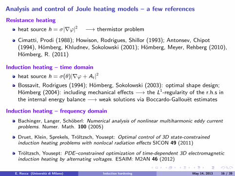
Analysis and control of Joule heating models ndash a few references
Resistance heating
heat source h = σ|nablaϕ|2 minusrarr thermistor problem
Cimatti Prodi (1988) Howison Rodrigues Shillor (1993) Antonsev Chipot(1994) Homberg Khludnev Sokolowski (2001) Homberg Meyer Rehberg (2010)Homberg R (2011)
Induction heating ndash time domain
heat source h = σ(θ)|nablaϕ+ At |2
Bossavit Rodrigues (1994) Homberg Sokolowski (2003) optimal shape designHomberg (2004) including mechanical effects minusrarr the L1-regularity of the rhs inthe internal energy balance minusrarr weak solutions via Boccardo-Gallouet estimates
Induction heating ndash frequency domain
Bachinger Langer Schoberl Numerical analysis of nonlinear multiharmonic eddy currentproblems Numer Math 100 (2005)
Druet Klein Sprekels Troltzsch Yousept Optimal control of 3D state-constrainedinduction heating problems with nonlocal radiation effects SICON 49 (2011)
Troltzsch Yousept PDEndashconstrained optimization of time-dependent 3D electromagneticinduction heating by alternating voltages ESAIM M2AN 46 (2012)
E Rocca (Universita di Milano) Induction hardening May 14 2013 16 39
Our results work in progess with D Hoemberg
Well-posedness of state system
Optimality conditions
E Rocca (Universita di Milano) Induction hardening May 14 2013 17 39
Our results work in progess with D Hoemberg
Well-posedness of state system
Optimality conditions
E Rocca (Universita di Milano) Induction hardening May 14 2013 17 39
Our results work in progess with D Hoemberg
Well-posedness of state system
Optimality conditions
E Rocca (Universita di Milano) Induction hardening May 14 2013 17 39
Solution space for vector potential
X =v isin L2(D)
∣∣∣ curl v isin L2(D) div v = 0 n times v∣∣∣partD
= 0
Assume partD isin C 11 Then X equipped with the norm
vX = curl vL2(D)
is a closed subspace of H1(D)
E Rocca (Universita di Milano) Induction hardening May 14 2013 18 39
Assumptions
(i) σ(x z) micro(x z) D times [0 1]rarr R are continuousand Lipschitz continuous (wrt z for almost allx isin D) function st
σ le σ(x z) le σ in D times [0 1]
micro le micro(x z) le micro in D times [0 1]
(ii) u isin H1(0T )
(iii) J0 D rarr R3 is an L2curl(D)-function
(iv) τ zeq isin C 2(R) and
τlowast le τ(θ) le τlowast 0 le zeq(θ) le 1
τC2(R) zeqC2(R) le M
| minus zeq(θ) + θz primeeq(θ)| |θz primeprimeeq(θ)| le M for all θ isin R
(v) g isin Linfin(0T Linfin(partΣ))
(vi) A0 isin X capH3(D) θ0 isinW 253(Σ)
E Rocca (Universita di Milano) Induction hardening May 14 2013 19 39
Weak formulation
Find a triple (A θ z) with the regularity properties
A isin H2(0T L2(D)) capW 1infin(0T X) curlA isin Linfin(0T L6(D)) (1)
θ isinW 153(0T L53(Σ)) cap L53(0T W 253(Σ)) cap L2(0T H1(Σ)) cap Linfin(Q) (2)
z isinW 1infin(0T W 1infin(Σ)) 0 le z lt 1 ae in Q (3)
solving the following systemintΩcupΣ
σ(x z)At middot v dx +
intD
1
micro(x z)curlA middot curl v dx =
intΩ
J0(x)u(t) middot v dx (4)
for all v isin X ae in (0T )
θt minus∆θ = minusF(θ z)zt + σ(x z)|At |2 ae in Q (5)
zt =1
τ(θ)(zeq(θ)minus z)+ ae in Q (6)
partθ
partν+ θ = g ae on partΣtimes (0T ) (7)
A(0) = A0 ae in D θ(0) = θ0 z(0) = 0 ae in Σ (8)
E Rocca (Universita di Milano) Induction hardening May 14 2013 20 39
Well-posedness result
Theorem 1 There exists a unique solution to (4)-(8) satisfying the regularities (1)-(3)and the following estimate
AH2(0T L2(D))capW 1infin(0T X) + curlALinfin(0T L6(D))
+ θW 153(0T L53(Σ))capL53(0T W 253(Σ))capL2(0T H1(Σ))capLinfin(Q) + zW 1infin(0T W 1infin(Σ)) le S
If we denote by (Ai θi zi ) (i = 1 2) two triples of solutions corresponding to data(A0i θ0i ui ) then there exists a positive constant C = C(S) such that the followingstability estimate holds true
(A1 minus A2)(t)2L2(D) + curl(A1 minus A2)2
L2(Dtimes(0T ))
+ partt(A1 minus A2)(t)2L2(D) + curl(partt(A1 minus A2))2
L2(Dtimes(0T ))
+ (θ1 minus θ2)(t)2L2(Σ) + θ1 minus θ22
L2(0T H1(Σ))
+ (z1 minus z2)(t)2H1(Σ) + partt(z1 minus z2)2
L2(0T H1(Σ))
le C(A01 minus A022
X + (partt(A1 minus A2))(0)2L2(D) + θ01 minus θ022
L2(Σ)
+u1J0 minus u2J02L2(0T ) + uprime1J0 minus uprime2J02
L2(0T )
)for all t isin [0T ]
E Rocca (Universita di Milano) Induction hardening May 14 2013 21 39
Well-posedness result
Theorem 1 There exists a unique solution to (4)-(8) satisfying the regularities (1)-(3)and the following estimate
AH2(0T L2(D))capW 1infin(0T X) + curlALinfin(0T L6(D))
+ θW 153(0T L53(Σ))capL53(0T W 253(Σ))capL2(0T H1(Σ))capLinfin(Q) + zW 1infin(0T W 1infin(Σ)) le S
If we denote by (Ai θi zi ) (i = 1 2) two triples of solutions corresponding to data(A0i θ0i ui ) then there exists a positive constant C = C(S) such that the followingstability estimate holds true
(A1 minus A2)(t)2L2(D) + curl(A1 minus A2)2
L2(Dtimes(0T ))
+ partt(A1 minus A2)(t)2L2(D) + curl(partt(A1 minus A2))2
L2(Dtimes(0T ))
+ (θ1 minus θ2)(t)2L2(Σ) + θ1 minus θ22
L2(0T H1(Σ))
+ (z1 minus z2)(t)2H1(Σ) + partt(z1 minus z2)2
L2(0T H1(Σ))
le C(A01 minus A022
X + (partt(A1 minus A2))(0)2L2(D) + θ01 minus θ022
L2(Σ)
+u1J0 minus u2J02L2(0T ) + uprime1J0 minus uprime2J02
L2(0T )
)for all t isin [0T ]
E Rocca (Universita di Milano) Induction hardening May 14 2013 21 39
Idea of the proof of Thm 1
Local existence via Shauder fixed point argument exploiting the Lipschitz continuityof the map θ 7rarr z from W 1p(0T0 Lp(Σ)) in itself
Global a-priori estimates on solutions1 Exploit the regularity and boundedness of the solution z to the ODE getting
zW 1infin(0T0Linfin(Σ)) le C 0 le z(x t) lt 1 ae in Q
2 Take first v = At then differentiate it (formally) in time and take v = At inintΩcupΣ
σ(x z)At middot v dx +
intD
1
micro(x z)curlA middot curl v dx =
intΩJ0(x)u(t) middot v dx
and use Est 1 and the assumptions on micro and σ getting
AH1(0T0X)capW 1infin(0T0L2(D)) + AtL103(Dtimes(0T0)) le C
3 Testθt minus∆θ = minusF(θ z)zt + σ(x z)|At |2
by θ and using maximal regularity results for parabolic equations we get
θL2(0T0H1(Σ))capLinfin(0T0L2(Σ))capL53(0T0W 253(Σ))capW 153(0T0L53(Σ)) le C
4 Differentiating (formally) the A-eq and taking v = Att arguing by comparison andusing the results of [Kawanago rsquo93] in order to prove the Linfin-estimate for θ we getthe desired regularity of solutions and we can prolpongate it over the whole timeinterval [0T ]
E Rocca (Universita di Milano) Induction hardening May 14 2013 22 39
Idea of the proof of Thm 1
Local existence via Shauder fixed point argument exploiting the Lipschitz continuityof the map θ 7rarr z from W 1p(0T0 Lp(Σ)) in itself
Global a-priori estimates on solutions1 Exploit the regularity and boundedness of the solution z to the ODE getting
zW 1infin(0T0Linfin(Σ)) le C 0 le z(x t) lt 1 ae in Q
2 Take first v = At then differentiate it (formally) in time and take v = At inintΩcupΣ
σ(x z)At middot v dx +
intD
1
micro(x z)curlA middot curl v dx =
intΩJ0(x)u(t) middot v dx
and use Est 1 and the assumptions on micro and σ getting
AH1(0T0X)capW 1infin(0T0L2(D)) + AtL103(Dtimes(0T0)) le C
3 Testθt minus∆θ = minusF(θ z)zt + σ(x z)|At |2
by θ and using maximal regularity results for parabolic equations we get
θL2(0T0H1(Σ))capLinfin(0T0L2(Σ))capL53(0T0W 253(Σ))capW 153(0T0L53(Σ)) le C
4 Differentiating (formally) the A-eq and taking v = Att arguing by comparison andusing the results of [Kawanago rsquo93] in order to prove the Linfin-estimate for θ we getthe desired regularity of solutions and we can prolpongate it over the whole timeinterval [0T ]
E Rocca (Universita di Milano) Induction hardening May 14 2013 22 39
Idea of the proof of Thm 1
Local existence via Shauder fixed point argument exploiting the Lipschitz continuityof the map θ 7rarr z from W 1p(0T0 Lp(Σ)) in itself
Global a-priori estimates on solutions1 Exploit the regularity and boundedness of the solution z to the ODE getting
zW 1infin(0T0Linfin(Σ)) le C 0 le z(x t) lt 1 ae in Q
2 Take first v = At then differentiate it (formally) in time and take v = At inintΩcupΣ
σ(x z)At middot v dx +
intD
1
micro(x z)curlA middot curl v dx =
intΩJ0(x)u(t) middot v dx
and use Est 1 and the assumptions on micro and σ getting
AH1(0T0X)capW 1infin(0T0L2(D)) + AtL103(Dtimes(0T0)) le C
3 Testθt minus∆θ = minusF(θ z)zt + σ(x z)|At |2
by θ and using maximal regularity results for parabolic equations we get
θL2(0T0H1(Σ))capLinfin(0T0L2(Σ))capL53(0T0W 253(Σ))capW 153(0T0L53(Σ)) le C
4 Differentiating (formally) the A-eq and taking v = Att arguing by comparison andusing the results of [Kawanago rsquo93] in order to prove the Linfin-estimate for θ we getthe desired regularity of solutions and we can prolpongate it over the whole timeinterval [0T ]
E Rocca (Universita di Milano) Induction hardening May 14 2013 22 39
Idea of the proof of Thm 1
Local existence via Shauder fixed point argument exploiting the Lipschitz continuityof the map θ 7rarr z from W 1p(0T0 Lp(Σ)) in itself
Global a-priori estimates on solutions1 Exploit the regularity and boundedness of the solution z to the ODE getting
zW 1infin(0T0Linfin(Σ)) le C 0 le z(x t) lt 1 ae in Q
2 Take first v = At then differentiate it (formally) in time and take v = At inintΩcupΣ
σ(x z)At middot v dx +
intD
1
micro(x z)curlA middot curl v dx =
intΩJ0(x)u(t) middot v dx
and use Est 1 and the assumptions on micro and σ getting
AH1(0T0X)capW 1infin(0T0L2(D)) + AtL103(Dtimes(0T0)) le C
3 Testθt minus∆θ = minusF(θ z)zt + σ(x z)|At |2
by θ and using maximal regularity results for parabolic equations we get
θL2(0T0H1(Σ))capLinfin(0T0L2(Σ))capL53(0T0W 253(Σ))capW 153(0T0L53(Σ)) le C
4 Differentiating (formally) the A-eq and taking v = Att arguing by comparison andusing the results of [Kawanago rsquo93] in order to prove the Linfin-estimate for θ we getthe desired regularity of solutions and we can prolpongate it over the whole timeinterval [0T ]
E Rocca (Universita di Milano) Induction hardening May 14 2013 22 39
Idea of the proof of Thm 1
Local existence via Shauder fixed point argument exploiting the Lipschitz continuityof the map θ 7rarr z from W 1p(0T0 Lp(Σ)) in itself
Global a-priori estimates on solutions1 Exploit the regularity and boundedness of the solution z to the ODE getting
zW 1infin(0T0Linfin(Σ)) le C 0 le z(x t) lt 1 ae in Q
2 Take first v = At then differentiate it (formally) in time and take v = At inintΩcupΣ
σ(x z)At middot v dx +
intD
1
micro(x z)curlA middot curl v dx =
intΩJ0(x)u(t) middot v dx
and use Est 1 and the assumptions on micro and σ getting
AH1(0T0X)capW 1infin(0T0L2(D)) + AtL103(Dtimes(0T0)) le C
3 Testθt minus∆θ = minusF(θ z)zt + σ(x z)|At |2
by θ and using maximal regularity results for parabolic equations we get
θL2(0T0H1(Σ))capLinfin(0T0L2(Σ))capL53(0T0W 253(Σ))capW 153(0T0L53(Σ)) le C
4 Differentiating (formally) the A-eq and taking v = Att arguing by comparison andusing the results of [Kawanago rsquo93] in order to prove the Linfin-estimate for θ we getthe desired regularity of solutions and we can prolpongate it over the whole timeinterval [0T ]
E Rocca (Universita di Milano) Induction hardening May 14 2013 22 39
Stability estimate
Differentiate in time equationintΩcupΣ
σ(x z)At middot v dx +
intD
1
micro(x z)curlA middot curl v dx =
intΩ
J0(x)u(t) middot v dx
and take the difference of the two differentiated relations in two solutions (Ai θi zi )and test the difference by (A1 minus A2)t
Use the Lipschitz continuity properties of the solution map to the ODE in z
Take the differences of the equations for θ and test by θ1 minus θ2 exploit the regularityof A and sum up the two relations
E Rocca (Universita di Milano) Induction hardening May 14 2013 23 39
Optimal control problem ndash Existence
cost functional
J (A θ z u) =β1
2
Tint0
intΣ
(θ(x t)minus θd(x t))2dxdt +
β2
2
intΣ
(z(x T )minus zd)2dx +β3
2u2
H1(0T )
control problem (CP)minJ (A θ z u)such that A θ z satisfies (P) and u isin Uad sub H1(0T )
Theorem 2 (CP) has a solution u isin Uad
E Rocca (Universita di Milano) Induction hardening May 14 2013 24 39
Optimal control problem ndash Existence
cost functional
J (A θ z u) =β1
2
Tint0
intΣ
(θ(x t)minus θd(x t))2dxdt +
β2
2
intΣ
(z(x T )minus zd)2dx +β3
2u2
H1(0T )
control problem (CP)minJ (A θ z u)such that A θ z satisfies (P) and u isin Uad sub H1(0T )
Theorem 2 (CP) has a solution u isin Uad
E Rocca (Universita di Milano) Induction hardening May 14 2013 24 39
Optimal control problem ndash Existence
cost functional
J (A θ z u) =β1
2
Tint0
intΣ
(θ(x t)minus θd(x t))2dxdt +
β2
2
intΣ
(z(x T )minus zd)2dx +β3
2u2
H1(0T )
control problem (CP)minJ (A θ z u)such that A θ z satisfies (P) and u isin Uad sub H1(0T )
Theorem 2 (CP) has a solution u isin Uad
E Rocca (Universita di Milano) Induction hardening May 14 2013 24 39
Optimal control problem ndash Differentiability
Lipschitz-continuity the control-to-state mapping
S u 7rarr (A θ z)
is Lipschitz continuous from H1(0T ) to Z by Theorem 1
Frechet differentiability the control-to-state mapping
S u 7rarr (A θ z)
is Frechet differentiable from H1(0T ) to Y Z sub Y
E Rocca (Universita di Milano) Induction hardening May 14 2013 25 39
Optimal control problem ndash First-order necessary conditions of optimality
adjoint systemminusσαt minus curl
( 1
microcurlα
)minus σprime(x z)ztα = minus2(σAtϑ)t
minusϑt minus k∆ϑ+ fθ(θ z)ϑ = fθζ + β1(θ minus θd)
minusζt minus fz(θ z)ζ + σprimeAt middotαminus σprime|At |2ϑ =microprime
micro2curlA middot curlαminus fzϑ
αtimes n = 0 in partD times (0T )
kpartϑ
partν+ κϑ = 0 in partΣtimes (0T )
ϑ(T ) = 0 ζ(T ) = z(x T )minus zd(x) in Σ
α(T ) = 0 in D
variational inequalityTint
0
(β3u(t)minus
intD
α(x t) middot J0(x t)dx)
(u minus u)dt
+
Tint0
β3uprime(t)(uprime(t)minus uprime(t))dt ge 0 for all u isin Uad sub H1(0T )
E Rocca (Universita di Milano) Induction hardening May 14 2013 26 39
Optimal control problem ndash First-order necessary conditions of optimality
adjoint systemminusσαt minus curl
( 1
microcurlα
)minus σprime(x z)ztα = minus2(σAtϑ)t
minusϑt minus k∆ϑ+ fθ(θ z)ϑ = fθζ + β1(θ minus θd)
minusζt minus fz(θ z)ζ + σprimeAt middotαminus σprime|At |2ϑ =microprime
micro2curlA middot curlαminus fzϑ
αtimes n = 0 in partD times (0T )
kpartϑ
partν+ κϑ = 0 in partΣtimes (0T )
ϑ(T ) = 0 ζ(T ) = z(x T )minus zd(x) in Σ
α(T ) = 0 in D
variational inequalityTint
0
(β3u(t)minus
intD
α(x t) middot J0(x t)dx)
(u minus u)dt
+
Tint0
β3uprime(t)(uprime(t)minus uprime(t))dt ge 0 for all u isin Uad sub H1(0T )
E Rocca (Universita di Milano) Induction hardening May 14 2013 26 39
Numerical results ndash Challenges [Homberg Petzold]
Multiple time scalesMagnetic vector potential and heat conductance live on different time scales(Averaging method)
Skin effectEddy currents are distributed in a small surface layer of the workpiece (Adaptivemesh generation)
Nonlinear material dataMagnetic permeability micro depends on temperature and magnetic field H(Linearization)
3DTime consuming simulation in 3D (Model reduction to tackle optimal controlproblem numerically)
E Rocca (Universita di Milano) Induction hardening May 14 2013 27 39
Numerical results ndash Challenges [Homberg Petzold]
Multiple time scalesMagnetic vector potential and heat conductance live on different time scales(Averaging method)
Skin effectEddy currents are distributed in a small surface layer of the workpiece (Adaptivemesh generation)
Nonlinear material dataMagnetic permeability micro depends on temperature and magnetic field H(Linearization)
3DTime consuming simulation in 3D (Model reduction to tackle optimal controlproblem numerically)
E Rocca (Universita di Milano) Induction hardening May 14 2013 27 39
Numerical results ndash Challenges [Homberg Petzold]
Multiple time scalesMagnetic vector potential and heat conductance live on different time scales(Averaging method)
Skin effectEddy currents are distributed in a small surface layer of the workpiece (Adaptivemesh generation)
Nonlinear material dataMagnetic permeability micro depends on temperature and magnetic field H(Linearization)
3DTime consuming simulation in 3D (Model reduction to tackle optimal controlproblem numerically)
E Rocca (Universita di Milano) Induction hardening May 14 2013 27 39
Numerical results ndash Challenges [Homberg Petzold]
Multiple time scalesMagnetic vector potential and heat conductance live on different time scales(Averaging method)
Skin effectEddy currents are distributed in a small surface layer of the workpiece (Adaptivemesh generation)
Nonlinear material dataMagnetic permeability micro depends on temperature and magnetic field H(Linearization)
3DTime consuming simulation in 3D (Model reduction to tackle optimal controlproblem numerically)
E Rocca (Universita di Milano) Induction hardening May 14 2013 27 39
Numerical realization ndash multiple time scales
Time scale for Maxwellrsquos equation governed by frequency of source currentf asymp 10 kHzminus 100 kHz consequetly τ sim 10minus5s
Time scale for heat equation governed by heat diffusion
τ sim cpρL2
kasymp 1 s
Alternating computation
I Solve for A with fixed temperature on fast time-scale
I Compute Joule heat by averaging electric energy Q = 1T
int T0 σ
∣∣∣ partApartt ∣∣∣2 dt
I Solve heat equation with fixed magnetic potential on slow time-scale (one time step)I Update A since σ and micro change with temperature
E Rocca (Universita di Milano) Induction hardening May 14 2013 28 39
Numerical realization ndash multiple time scales
Time scale for Maxwellrsquos equation governed by frequency of source currentf asymp 10 kHzminus 100 kHz consequetly τ sim 10minus5s
Time scale for heat equation governed by heat diffusion
τ sim cpρL2
kasymp 1 s
Alternating computation
I Solve for A with fixed temperature on fast time-scale
I Compute Joule heat by averaging electric energy Q = 1T
int T0 σ
∣∣∣ partApartt ∣∣∣2 dt
I Solve heat equation with fixed magnetic potential on slow time-scale (one time step)I Update A since σ and micro change with temperature
E Rocca (Universita di Milano) Induction hardening May 14 2013 28 39
Thermal and electrical conductivity heat capacity and density
Material data depend on temperature
Electrical conductivity σ(θ)Thermal conductivity κ(θ)
Density ρ(θ)Specific heat capacity cp(θ)
Nonlinear relation between magnetic induction B and magnetic field HMagnetization curve B = micro(θH)H
E Rocca (Universita di Milano) Induction hardening May 14 2013 29 39
Example 1 HF temperature and growth of austenite
(Video austenitemp4)
Figure temperature and austenite growth at high frequency
E Rocca (Universita di Milano) Induction hardening May 14 2013 30 39

Our results work in progess with D Hoemberg
Well-posedness of state system
Optimality conditions
E Rocca (Universita di Milano) Induction hardening May 14 2013 17 39
Our results work in progess with D Hoemberg
Well-posedness of state system
Optimality conditions
E Rocca (Universita di Milano) Induction hardening May 14 2013 17 39
Our results work in progess with D Hoemberg
Well-posedness of state system
Optimality conditions
E Rocca (Universita di Milano) Induction hardening May 14 2013 17 39
Solution space for vector potential
X =v isin L2(D)
∣∣∣ curl v isin L2(D) div v = 0 n times v∣∣∣partD
= 0
Assume partD isin C 11 Then X equipped with the norm
vX = curl vL2(D)
is a closed subspace of H1(D)
E Rocca (Universita di Milano) Induction hardening May 14 2013 18 39
Assumptions
(i) σ(x z) micro(x z) D times [0 1]rarr R are continuousand Lipschitz continuous (wrt z for almost allx isin D) function st
σ le σ(x z) le σ in D times [0 1]
micro le micro(x z) le micro in D times [0 1]
(ii) u isin H1(0T )
(iii) J0 D rarr R3 is an L2curl(D)-function
(iv) τ zeq isin C 2(R) and
τlowast le τ(θ) le τlowast 0 le zeq(θ) le 1
τC2(R) zeqC2(R) le M
| minus zeq(θ) + θz primeeq(θ)| |θz primeprimeeq(θ)| le M for all θ isin R
(v) g isin Linfin(0T Linfin(partΣ))
(vi) A0 isin X capH3(D) θ0 isinW 253(Σ)
E Rocca (Universita di Milano) Induction hardening May 14 2013 19 39
Weak formulation
Find a triple (A θ z) with the regularity properties
A isin H2(0T L2(D)) capW 1infin(0T X) curlA isin Linfin(0T L6(D)) (1)
θ isinW 153(0T L53(Σ)) cap L53(0T W 253(Σ)) cap L2(0T H1(Σ)) cap Linfin(Q) (2)
z isinW 1infin(0T W 1infin(Σ)) 0 le z lt 1 ae in Q (3)
solving the following systemintΩcupΣ
σ(x z)At middot v dx +
intD
1
micro(x z)curlA middot curl v dx =
intΩ
J0(x)u(t) middot v dx (4)
for all v isin X ae in (0T )
θt minus∆θ = minusF(θ z)zt + σ(x z)|At |2 ae in Q (5)
zt =1
τ(θ)(zeq(θ)minus z)+ ae in Q (6)
partθ
partν+ θ = g ae on partΣtimes (0T ) (7)
A(0) = A0 ae in D θ(0) = θ0 z(0) = 0 ae in Σ (8)
E Rocca (Universita di Milano) Induction hardening May 14 2013 20 39
Well-posedness result
Theorem 1 There exists a unique solution to (4)-(8) satisfying the regularities (1)-(3)and the following estimate
AH2(0T L2(D))capW 1infin(0T X) + curlALinfin(0T L6(D))
+ θW 153(0T L53(Σ))capL53(0T W 253(Σ))capL2(0T H1(Σ))capLinfin(Q) + zW 1infin(0T W 1infin(Σ)) le S
If we denote by (Ai θi zi ) (i = 1 2) two triples of solutions corresponding to data(A0i θ0i ui ) then there exists a positive constant C = C(S) such that the followingstability estimate holds true
(A1 minus A2)(t)2L2(D) + curl(A1 minus A2)2
L2(Dtimes(0T ))
+ partt(A1 minus A2)(t)2L2(D) + curl(partt(A1 minus A2))2
L2(Dtimes(0T ))
+ (θ1 minus θ2)(t)2L2(Σ) + θ1 minus θ22
L2(0T H1(Σ))
+ (z1 minus z2)(t)2H1(Σ) + partt(z1 minus z2)2
L2(0T H1(Σ))
le C(A01 minus A022
X + (partt(A1 minus A2))(0)2L2(D) + θ01 minus θ022
L2(Σ)
+u1J0 minus u2J02L2(0T ) + uprime1J0 minus uprime2J02
L2(0T )
)for all t isin [0T ]
E Rocca (Universita di Milano) Induction hardening May 14 2013 21 39
Well-posedness result
Theorem 1 There exists a unique solution to (4)-(8) satisfying the regularities (1)-(3)and the following estimate
AH2(0T L2(D))capW 1infin(0T X) + curlALinfin(0T L6(D))
+ θW 153(0T L53(Σ))capL53(0T W 253(Σ))capL2(0T H1(Σ))capLinfin(Q) + zW 1infin(0T W 1infin(Σ)) le S
If we denote by (Ai θi zi ) (i = 1 2) two triples of solutions corresponding to data(A0i θ0i ui ) then there exists a positive constant C = C(S) such that the followingstability estimate holds true
(A1 minus A2)(t)2L2(D) + curl(A1 minus A2)2
L2(Dtimes(0T ))
+ partt(A1 minus A2)(t)2L2(D) + curl(partt(A1 minus A2))2
L2(Dtimes(0T ))
+ (θ1 minus θ2)(t)2L2(Σ) + θ1 minus θ22
L2(0T H1(Σ))
+ (z1 minus z2)(t)2H1(Σ) + partt(z1 minus z2)2
L2(0T H1(Σ))
le C(A01 minus A022
X + (partt(A1 minus A2))(0)2L2(D) + θ01 minus θ022
L2(Σ)
+u1J0 minus u2J02L2(0T ) + uprime1J0 minus uprime2J02
L2(0T )
)for all t isin [0T ]
E Rocca (Universita di Milano) Induction hardening May 14 2013 21 39
Idea of the proof of Thm 1
Local existence via Shauder fixed point argument exploiting the Lipschitz continuityof the map θ 7rarr z from W 1p(0T0 Lp(Σ)) in itself
Global a-priori estimates on solutions1 Exploit the regularity and boundedness of the solution z to the ODE getting
zW 1infin(0T0Linfin(Σ)) le C 0 le z(x t) lt 1 ae in Q
2 Take first v = At then differentiate it (formally) in time and take v = At inintΩcupΣ
σ(x z)At middot v dx +
intD
1
micro(x z)curlA middot curl v dx =
intΩJ0(x)u(t) middot v dx
and use Est 1 and the assumptions on micro and σ getting
AH1(0T0X)capW 1infin(0T0L2(D)) + AtL103(Dtimes(0T0)) le C
3 Testθt minus∆θ = minusF(θ z)zt + σ(x z)|At |2
by θ and using maximal regularity results for parabolic equations we get
θL2(0T0H1(Σ))capLinfin(0T0L2(Σ))capL53(0T0W 253(Σ))capW 153(0T0L53(Σ)) le C
4 Differentiating (formally) the A-eq and taking v = Att arguing by comparison andusing the results of [Kawanago rsquo93] in order to prove the Linfin-estimate for θ we getthe desired regularity of solutions and we can prolpongate it over the whole timeinterval [0T ]
E Rocca (Universita di Milano) Induction hardening May 14 2013 22 39
Idea of the proof of Thm 1
Local existence via Shauder fixed point argument exploiting the Lipschitz continuityof the map θ 7rarr z from W 1p(0T0 Lp(Σ)) in itself
Global a-priori estimates on solutions1 Exploit the regularity and boundedness of the solution z to the ODE getting
zW 1infin(0T0Linfin(Σ)) le C 0 le z(x t) lt 1 ae in Q
2 Take first v = At then differentiate it (formally) in time and take v = At inintΩcupΣ
σ(x z)At middot v dx +
intD
1
micro(x z)curlA middot curl v dx =
intΩJ0(x)u(t) middot v dx
and use Est 1 and the assumptions on micro and σ getting
AH1(0T0X)capW 1infin(0T0L2(D)) + AtL103(Dtimes(0T0)) le C
3 Testθt minus∆θ = minusF(θ z)zt + σ(x z)|At |2
by θ and using maximal regularity results for parabolic equations we get
θL2(0T0H1(Σ))capLinfin(0T0L2(Σ))capL53(0T0W 253(Σ))capW 153(0T0L53(Σ)) le C
4 Differentiating (formally) the A-eq and taking v = Att arguing by comparison andusing the results of [Kawanago rsquo93] in order to prove the Linfin-estimate for θ we getthe desired regularity of solutions and we can prolpongate it over the whole timeinterval [0T ]
E Rocca (Universita di Milano) Induction hardening May 14 2013 22 39
Idea of the proof of Thm 1
Local existence via Shauder fixed point argument exploiting the Lipschitz continuityof the map θ 7rarr z from W 1p(0T0 Lp(Σ)) in itself
Global a-priori estimates on solutions1 Exploit the regularity and boundedness of the solution z to the ODE getting
zW 1infin(0T0Linfin(Σ)) le C 0 le z(x t) lt 1 ae in Q
2 Take first v = At then differentiate it (formally) in time and take v = At inintΩcupΣ
σ(x z)At middot v dx +
intD
1
micro(x z)curlA middot curl v dx =
intΩJ0(x)u(t) middot v dx
and use Est 1 and the assumptions on micro and σ getting
AH1(0T0X)capW 1infin(0T0L2(D)) + AtL103(Dtimes(0T0)) le C
3 Testθt minus∆θ = minusF(θ z)zt + σ(x z)|At |2
by θ and using maximal regularity results for parabolic equations we get
θL2(0T0H1(Σ))capLinfin(0T0L2(Σ))capL53(0T0W 253(Σ))capW 153(0T0L53(Σ)) le C
4 Differentiating (formally) the A-eq and taking v = Att arguing by comparison andusing the results of [Kawanago rsquo93] in order to prove the Linfin-estimate for θ we getthe desired regularity of solutions and we can prolpongate it over the whole timeinterval [0T ]
E Rocca (Universita di Milano) Induction hardening May 14 2013 22 39
Idea of the proof of Thm 1
Local existence via Shauder fixed point argument exploiting the Lipschitz continuityof the map θ 7rarr z from W 1p(0T0 Lp(Σ)) in itself
Global a-priori estimates on solutions1 Exploit the regularity and boundedness of the solution z to the ODE getting
zW 1infin(0T0Linfin(Σ)) le C 0 le z(x t) lt 1 ae in Q
2 Take first v = At then differentiate it (formally) in time and take v = At inintΩcupΣ
σ(x z)At middot v dx +
intD
1
micro(x z)curlA middot curl v dx =
intΩJ0(x)u(t) middot v dx
and use Est 1 and the assumptions on micro and σ getting
AH1(0T0X)capW 1infin(0T0L2(D)) + AtL103(Dtimes(0T0)) le C
3 Testθt minus∆θ = minusF(θ z)zt + σ(x z)|At |2
by θ and using maximal regularity results for parabolic equations we get
θL2(0T0H1(Σ))capLinfin(0T0L2(Σ))capL53(0T0W 253(Σ))capW 153(0T0L53(Σ)) le C
4 Differentiating (formally) the A-eq and taking v = Att arguing by comparison andusing the results of [Kawanago rsquo93] in order to prove the Linfin-estimate for θ we getthe desired regularity of solutions and we can prolpongate it over the whole timeinterval [0T ]
E Rocca (Universita di Milano) Induction hardening May 14 2013 22 39
Idea of the proof of Thm 1
Local existence via Shauder fixed point argument exploiting the Lipschitz continuityof the map θ 7rarr z from W 1p(0T0 Lp(Σ)) in itself
Global a-priori estimates on solutions1 Exploit the regularity and boundedness of the solution z to the ODE getting
zW 1infin(0T0Linfin(Σ)) le C 0 le z(x t) lt 1 ae in Q
2 Take first v = At then differentiate it (formally) in time and take v = At inintΩcupΣ
σ(x z)At middot v dx +
intD
1
micro(x z)curlA middot curl v dx =
intΩJ0(x)u(t) middot v dx
and use Est 1 and the assumptions on micro and σ getting
AH1(0T0X)capW 1infin(0T0L2(D)) + AtL103(Dtimes(0T0)) le C
3 Testθt minus∆θ = minusF(θ z)zt + σ(x z)|At |2
by θ and using maximal regularity results for parabolic equations we get
θL2(0T0H1(Σ))capLinfin(0T0L2(Σ))capL53(0T0W 253(Σ))capW 153(0T0L53(Σ)) le C
4 Differentiating (formally) the A-eq and taking v = Att arguing by comparison andusing the results of [Kawanago rsquo93] in order to prove the Linfin-estimate for θ we getthe desired regularity of solutions and we can prolpongate it over the whole timeinterval [0T ]
E Rocca (Universita di Milano) Induction hardening May 14 2013 22 39
Stability estimate
Differentiate in time equationintΩcupΣ
σ(x z)At middot v dx +
intD
1
micro(x z)curlA middot curl v dx =
intΩ
J0(x)u(t) middot v dx
and take the difference of the two differentiated relations in two solutions (Ai θi zi )and test the difference by (A1 minus A2)t
Use the Lipschitz continuity properties of the solution map to the ODE in z
Take the differences of the equations for θ and test by θ1 minus θ2 exploit the regularityof A and sum up the two relations
E Rocca (Universita di Milano) Induction hardening May 14 2013 23 39
Optimal control problem ndash Existence
cost functional
J (A θ z u) =β1
2
Tint0
intΣ
(θ(x t)minus θd(x t))2dxdt +
β2
2
intΣ
(z(x T )minus zd)2dx +β3
2u2
H1(0T )
control problem (CP)minJ (A θ z u)such that A θ z satisfies (P) and u isin Uad sub H1(0T )
Theorem 2 (CP) has a solution u isin Uad
E Rocca (Universita di Milano) Induction hardening May 14 2013 24 39
Optimal control problem ndash Existence
cost functional
J (A θ z u) =β1
2
Tint0
intΣ
(θ(x t)minus θd(x t))2dxdt +
β2
2
intΣ
(z(x T )minus zd)2dx +β3
2u2
H1(0T )
control problem (CP)minJ (A θ z u)such that A θ z satisfies (P) and u isin Uad sub H1(0T )
Theorem 2 (CP) has a solution u isin Uad
E Rocca (Universita di Milano) Induction hardening May 14 2013 24 39
Optimal control problem ndash Existence
cost functional
J (A θ z u) =β1
2
Tint0
intΣ
(θ(x t)minus θd(x t))2dxdt +
β2
2
intΣ
(z(x T )minus zd)2dx +β3
2u2
H1(0T )
control problem (CP)minJ (A θ z u)such that A θ z satisfies (P) and u isin Uad sub H1(0T )
Theorem 2 (CP) has a solution u isin Uad
E Rocca (Universita di Milano) Induction hardening May 14 2013 24 39
Optimal control problem ndash Differentiability
Lipschitz-continuity the control-to-state mapping
S u 7rarr (A θ z)
is Lipschitz continuous from H1(0T ) to Z by Theorem 1
Frechet differentiability the control-to-state mapping
S u 7rarr (A θ z)
is Frechet differentiable from H1(0T ) to Y Z sub Y
E Rocca (Universita di Milano) Induction hardening May 14 2013 25 39
Optimal control problem ndash First-order necessary conditions of optimality
adjoint systemminusσαt minus curl
( 1
microcurlα
)minus σprime(x z)ztα = minus2(σAtϑ)t
minusϑt minus k∆ϑ+ fθ(θ z)ϑ = fθζ + β1(θ minus θd)
minusζt minus fz(θ z)ζ + σprimeAt middotαminus σprime|At |2ϑ =microprime
micro2curlA middot curlαminus fzϑ
αtimes n = 0 in partD times (0T )
kpartϑ
partν+ κϑ = 0 in partΣtimes (0T )
ϑ(T ) = 0 ζ(T ) = z(x T )minus zd(x) in Σ
α(T ) = 0 in D
variational inequalityTint
0
(β3u(t)minus
intD
α(x t) middot J0(x t)dx)
(u minus u)dt
+
Tint0
β3uprime(t)(uprime(t)minus uprime(t))dt ge 0 for all u isin Uad sub H1(0T )
E Rocca (Universita di Milano) Induction hardening May 14 2013 26 39
Optimal control problem ndash First-order necessary conditions of optimality
adjoint systemminusσαt minus curl
( 1
microcurlα
)minus σprime(x z)ztα = minus2(σAtϑ)t
minusϑt minus k∆ϑ+ fθ(θ z)ϑ = fθζ + β1(θ minus θd)
minusζt minus fz(θ z)ζ + σprimeAt middotαminus σprime|At |2ϑ =microprime
micro2curlA middot curlαminus fzϑ
αtimes n = 0 in partD times (0T )
kpartϑ
partν+ κϑ = 0 in partΣtimes (0T )
ϑ(T ) = 0 ζ(T ) = z(x T )minus zd(x) in Σ
α(T ) = 0 in D
variational inequalityTint
0
(β3u(t)minus
intD
α(x t) middot J0(x t)dx)
(u minus u)dt
+
Tint0
β3uprime(t)(uprime(t)minus uprime(t))dt ge 0 for all u isin Uad sub H1(0T )
E Rocca (Universita di Milano) Induction hardening May 14 2013 26 39
Numerical results ndash Challenges [Homberg Petzold]
Multiple time scalesMagnetic vector potential and heat conductance live on different time scales(Averaging method)
Skin effectEddy currents are distributed in a small surface layer of the workpiece (Adaptivemesh generation)
Nonlinear material dataMagnetic permeability micro depends on temperature and magnetic field H(Linearization)
3DTime consuming simulation in 3D (Model reduction to tackle optimal controlproblem numerically)
E Rocca (Universita di Milano) Induction hardening May 14 2013 27 39
Numerical results ndash Challenges [Homberg Petzold]
Multiple time scalesMagnetic vector potential and heat conductance live on different time scales(Averaging method)
Skin effectEddy currents are distributed in a small surface layer of the workpiece (Adaptivemesh generation)
Nonlinear material dataMagnetic permeability micro depends on temperature and magnetic field H(Linearization)
3DTime consuming simulation in 3D (Model reduction to tackle optimal controlproblem numerically)
E Rocca (Universita di Milano) Induction hardening May 14 2013 27 39
Numerical results ndash Challenges [Homberg Petzold]
Multiple time scalesMagnetic vector potential and heat conductance live on different time scales(Averaging method)
Skin effectEddy currents are distributed in a small surface layer of the workpiece (Adaptivemesh generation)
Nonlinear material dataMagnetic permeability micro depends on temperature and magnetic field H(Linearization)
3DTime consuming simulation in 3D (Model reduction to tackle optimal controlproblem numerically)
E Rocca (Universita di Milano) Induction hardening May 14 2013 27 39
Numerical results ndash Challenges [Homberg Petzold]
Multiple time scalesMagnetic vector potential and heat conductance live on different time scales(Averaging method)
Skin effectEddy currents are distributed in a small surface layer of the workpiece (Adaptivemesh generation)
Nonlinear material dataMagnetic permeability micro depends on temperature and magnetic field H(Linearization)
3DTime consuming simulation in 3D (Model reduction to tackle optimal controlproblem numerically)
E Rocca (Universita di Milano) Induction hardening May 14 2013 27 39
Numerical realization ndash multiple time scales
Time scale for Maxwellrsquos equation governed by frequency of source currentf asymp 10 kHzminus 100 kHz consequetly τ sim 10minus5s
Time scale for heat equation governed by heat diffusion
τ sim cpρL2
kasymp 1 s
Alternating computation
I Solve for A with fixed temperature on fast time-scale
I Compute Joule heat by averaging electric energy Q = 1T
int T0 σ
∣∣∣ partApartt ∣∣∣2 dt
I Solve heat equation with fixed magnetic potential on slow time-scale (one time step)I Update A since σ and micro change with temperature
E Rocca (Universita di Milano) Induction hardening May 14 2013 28 39
Numerical realization ndash multiple time scales
Time scale for Maxwellrsquos equation governed by frequency of source currentf asymp 10 kHzminus 100 kHz consequetly τ sim 10minus5s
Time scale for heat equation governed by heat diffusion
τ sim cpρL2
kasymp 1 s
Alternating computation
I Solve for A with fixed temperature on fast time-scale
I Compute Joule heat by averaging electric energy Q = 1T
int T0 σ
∣∣∣ partApartt ∣∣∣2 dt
I Solve heat equation with fixed magnetic potential on slow time-scale (one time step)I Update A since σ and micro change with temperature
E Rocca (Universita di Milano) Induction hardening May 14 2013 28 39
Thermal and electrical conductivity heat capacity and density
Material data depend on temperature
Electrical conductivity σ(θ)Thermal conductivity κ(θ)
Density ρ(θ)Specific heat capacity cp(θ)
Nonlinear relation between magnetic induction B and magnetic field HMagnetization curve B = micro(θH)H
E Rocca (Universita di Milano) Induction hardening May 14 2013 29 39
Example 1 HF temperature and growth of austenite
(Video austenitemp4)
Figure temperature and austenite growth at high frequency
E Rocca (Universita di Milano) Induction hardening May 14 2013 30 39

Our results work in progess with D Hoemberg
Well-posedness of state system
Optimality conditions
E Rocca (Universita di Milano) Induction hardening May 14 2013 17 39
Our results work in progess with D Hoemberg
Well-posedness of state system
Optimality conditions
E Rocca (Universita di Milano) Induction hardening May 14 2013 17 39
Solution space for vector potential
X =v isin L2(D)
∣∣∣ curl v isin L2(D) div v = 0 n times v∣∣∣partD
= 0
Assume partD isin C 11 Then X equipped with the norm
vX = curl vL2(D)
is a closed subspace of H1(D)
E Rocca (Universita di Milano) Induction hardening May 14 2013 18 39
Assumptions
(i) σ(x z) micro(x z) D times [0 1]rarr R are continuousand Lipschitz continuous (wrt z for almost allx isin D) function st
σ le σ(x z) le σ in D times [0 1]
micro le micro(x z) le micro in D times [0 1]
(ii) u isin H1(0T )
(iii) J0 D rarr R3 is an L2curl(D)-function
(iv) τ zeq isin C 2(R) and
τlowast le τ(θ) le τlowast 0 le zeq(θ) le 1
τC2(R) zeqC2(R) le M
| minus zeq(θ) + θz primeeq(θ)| |θz primeprimeeq(θ)| le M for all θ isin R
(v) g isin Linfin(0T Linfin(partΣ))
(vi) A0 isin X capH3(D) θ0 isinW 253(Σ)
E Rocca (Universita di Milano) Induction hardening May 14 2013 19 39
Weak formulation
Find a triple (A θ z) with the regularity properties
A isin H2(0T L2(D)) capW 1infin(0T X) curlA isin Linfin(0T L6(D)) (1)
θ isinW 153(0T L53(Σ)) cap L53(0T W 253(Σ)) cap L2(0T H1(Σ)) cap Linfin(Q) (2)
z isinW 1infin(0T W 1infin(Σ)) 0 le z lt 1 ae in Q (3)
solving the following systemintΩcupΣ
σ(x z)At middot v dx +
intD
1
micro(x z)curlA middot curl v dx =
intΩ
J0(x)u(t) middot v dx (4)
for all v isin X ae in (0T )
θt minus∆θ = minusF(θ z)zt + σ(x z)|At |2 ae in Q (5)
zt =1
τ(θ)(zeq(θ)minus z)+ ae in Q (6)
partθ
partν+ θ = g ae on partΣtimes (0T ) (7)
A(0) = A0 ae in D θ(0) = θ0 z(0) = 0 ae in Σ (8)
E Rocca (Universita di Milano) Induction hardening May 14 2013 20 39
Well-posedness result
Theorem 1 There exists a unique solution to (4)-(8) satisfying the regularities (1)-(3)and the following estimate
AH2(0T L2(D))capW 1infin(0T X) + curlALinfin(0T L6(D))
+ θW 153(0T L53(Σ))capL53(0T W 253(Σ))capL2(0T H1(Σ))capLinfin(Q) + zW 1infin(0T W 1infin(Σ)) le S
If we denote by (Ai θi zi ) (i = 1 2) two triples of solutions corresponding to data(A0i θ0i ui ) then there exists a positive constant C = C(S) such that the followingstability estimate holds true
(A1 minus A2)(t)2L2(D) + curl(A1 minus A2)2
L2(Dtimes(0T ))
+ partt(A1 minus A2)(t)2L2(D) + curl(partt(A1 minus A2))2
L2(Dtimes(0T ))
+ (θ1 minus θ2)(t)2L2(Σ) + θ1 minus θ22
L2(0T H1(Σ))
+ (z1 minus z2)(t)2H1(Σ) + partt(z1 minus z2)2
L2(0T H1(Σ))
le C(A01 minus A022
X + (partt(A1 minus A2))(0)2L2(D) + θ01 minus θ022
L2(Σ)
+u1J0 minus u2J02L2(0T ) + uprime1J0 minus uprime2J02
L2(0T )
)for all t isin [0T ]
E Rocca (Universita di Milano) Induction hardening May 14 2013 21 39
Well-posedness result
Theorem 1 There exists a unique solution to (4)-(8) satisfying the regularities (1)-(3)and the following estimate
AH2(0T L2(D))capW 1infin(0T X) + curlALinfin(0T L6(D))
+ θW 153(0T L53(Σ))capL53(0T W 253(Σ))capL2(0T H1(Σ))capLinfin(Q) + zW 1infin(0T W 1infin(Σ)) le S
If we denote by (Ai θi zi ) (i = 1 2) two triples of solutions corresponding to data(A0i θ0i ui ) then there exists a positive constant C = C(S) such that the followingstability estimate holds true
(A1 minus A2)(t)2L2(D) + curl(A1 minus A2)2
L2(Dtimes(0T ))
+ partt(A1 minus A2)(t)2L2(D) + curl(partt(A1 minus A2))2
L2(Dtimes(0T ))
+ (θ1 minus θ2)(t)2L2(Σ) + θ1 minus θ22
L2(0T H1(Σ))
+ (z1 minus z2)(t)2H1(Σ) + partt(z1 minus z2)2
L2(0T H1(Σ))
le C(A01 minus A022
X + (partt(A1 minus A2))(0)2L2(D) + θ01 minus θ022
L2(Σ)
+u1J0 minus u2J02L2(0T ) + uprime1J0 minus uprime2J02
L2(0T )
)for all t isin [0T ]
E Rocca (Universita di Milano) Induction hardening May 14 2013 21 39
Idea of the proof of Thm 1
Local existence via Shauder fixed point argument exploiting the Lipschitz continuityof the map θ 7rarr z from W 1p(0T0 Lp(Σ)) in itself
Global a-priori estimates on solutions1 Exploit the regularity and boundedness of the solution z to the ODE getting
zW 1infin(0T0Linfin(Σ)) le C 0 le z(x t) lt 1 ae in Q
2 Take first v = At then differentiate it (formally) in time and take v = At inintΩcupΣ
σ(x z)At middot v dx +
intD
1
micro(x z)curlA middot curl v dx =
intΩJ0(x)u(t) middot v dx
and use Est 1 and the assumptions on micro and σ getting
AH1(0T0X)capW 1infin(0T0L2(D)) + AtL103(Dtimes(0T0)) le C
3 Testθt minus∆θ = minusF(θ z)zt + σ(x z)|At |2
by θ and using maximal regularity results for parabolic equations we get
θL2(0T0H1(Σ))capLinfin(0T0L2(Σ))capL53(0T0W 253(Σ))capW 153(0T0L53(Σ)) le C
4 Differentiating (formally) the A-eq and taking v = Att arguing by comparison andusing the results of [Kawanago rsquo93] in order to prove the Linfin-estimate for θ we getthe desired regularity of solutions and we can prolpongate it over the whole timeinterval [0T ]
E Rocca (Universita di Milano) Induction hardening May 14 2013 22 39
Idea of the proof of Thm 1
Local existence via Shauder fixed point argument exploiting the Lipschitz continuityof the map θ 7rarr z from W 1p(0T0 Lp(Σ)) in itself
Global a-priori estimates on solutions1 Exploit the regularity and boundedness of the solution z to the ODE getting
zW 1infin(0T0Linfin(Σ)) le C 0 le z(x t) lt 1 ae in Q
2 Take first v = At then differentiate it (formally) in time and take v = At inintΩcupΣ
σ(x z)At middot v dx +
intD
1
micro(x z)curlA middot curl v dx =
intΩJ0(x)u(t) middot v dx
and use Est 1 and the assumptions on micro and σ getting
AH1(0T0X)capW 1infin(0T0L2(D)) + AtL103(Dtimes(0T0)) le C
3 Testθt minus∆θ = minusF(θ z)zt + σ(x z)|At |2
by θ and using maximal regularity results for parabolic equations we get
θL2(0T0H1(Σ))capLinfin(0T0L2(Σ))capL53(0T0W 253(Σ))capW 153(0T0L53(Σ)) le C
4 Differentiating (formally) the A-eq and taking v = Att arguing by comparison andusing the results of [Kawanago rsquo93] in order to prove the Linfin-estimate for θ we getthe desired regularity of solutions and we can prolpongate it over the whole timeinterval [0T ]
E Rocca (Universita di Milano) Induction hardening May 14 2013 22 39
Idea of the proof of Thm 1
Local existence via Shauder fixed point argument exploiting the Lipschitz continuityof the map θ 7rarr z from W 1p(0T0 Lp(Σ)) in itself
Global a-priori estimates on solutions1 Exploit the regularity and boundedness of the solution z to the ODE getting
zW 1infin(0T0Linfin(Σ)) le C 0 le z(x t) lt 1 ae in Q
2 Take first v = At then differentiate it (formally) in time and take v = At inintΩcupΣ
σ(x z)At middot v dx +
intD
1
micro(x z)curlA middot curl v dx =
intΩJ0(x)u(t) middot v dx
and use Est 1 and the assumptions on micro and σ getting
AH1(0T0X)capW 1infin(0T0L2(D)) + AtL103(Dtimes(0T0)) le C
3 Testθt minus∆θ = minusF(θ z)zt + σ(x z)|At |2
by θ and using maximal regularity results for parabolic equations we get
θL2(0T0H1(Σ))capLinfin(0T0L2(Σ))capL53(0T0W 253(Σ))capW 153(0T0L53(Σ)) le C
4 Differentiating (formally) the A-eq and taking v = Att arguing by comparison andusing the results of [Kawanago rsquo93] in order to prove the Linfin-estimate for θ we getthe desired regularity of solutions and we can prolpongate it over the whole timeinterval [0T ]
E Rocca (Universita di Milano) Induction hardening May 14 2013 22 39
Idea of the proof of Thm 1
Local existence via Shauder fixed point argument exploiting the Lipschitz continuityof the map θ 7rarr z from W 1p(0T0 Lp(Σ)) in itself
Global a-priori estimates on solutions1 Exploit the regularity and boundedness of the solution z to the ODE getting
zW 1infin(0T0Linfin(Σ)) le C 0 le z(x t) lt 1 ae in Q
2 Take first v = At then differentiate it (formally) in time and take v = At inintΩcupΣ
σ(x z)At middot v dx +
intD
1
micro(x z)curlA middot curl v dx =
intΩJ0(x)u(t) middot v dx
and use Est 1 and the assumptions on micro and σ getting
AH1(0T0X)capW 1infin(0T0L2(D)) + AtL103(Dtimes(0T0)) le C
3 Testθt minus∆θ = minusF(θ z)zt + σ(x z)|At |2
by θ and using maximal regularity results for parabolic equations we get
θL2(0T0H1(Σ))capLinfin(0T0L2(Σ))capL53(0T0W 253(Σ))capW 153(0T0L53(Σ)) le C
4 Differentiating (formally) the A-eq and taking v = Att arguing by comparison andusing the results of [Kawanago rsquo93] in order to prove the Linfin-estimate for θ we getthe desired regularity of solutions and we can prolpongate it over the whole timeinterval [0T ]
E Rocca (Universita di Milano) Induction hardening May 14 2013 22 39
Idea of the proof of Thm 1
Local existence via Shauder fixed point argument exploiting the Lipschitz continuityof the map θ 7rarr z from W 1p(0T0 Lp(Σ)) in itself
Global a-priori estimates on solutions1 Exploit the regularity and boundedness of the solution z to the ODE getting
zW 1infin(0T0Linfin(Σ)) le C 0 le z(x t) lt 1 ae in Q
2 Take first v = At then differentiate it (formally) in time and take v = At inintΩcupΣ
σ(x z)At middot v dx +
intD
1
micro(x z)curlA middot curl v dx =
intΩJ0(x)u(t) middot v dx
and use Est 1 and the assumptions on micro and σ getting
AH1(0T0X)capW 1infin(0T0L2(D)) + AtL103(Dtimes(0T0)) le C
3 Testθt minus∆θ = minusF(θ z)zt + σ(x z)|At |2
by θ and using maximal regularity results for parabolic equations we get
θL2(0T0H1(Σ))capLinfin(0T0L2(Σ))capL53(0T0W 253(Σ))capW 153(0T0L53(Σ)) le C
4 Differentiating (formally) the A-eq and taking v = Att arguing by comparison andusing the results of [Kawanago rsquo93] in order to prove the Linfin-estimate for θ we getthe desired regularity of solutions and we can prolpongate it over the whole timeinterval [0T ]
E Rocca (Universita di Milano) Induction hardening May 14 2013 22 39
Stability estimate
Differentiate in time equationintΩcupΣ
σ(x z)At middot v dx +
intD
1
micro(x z)curlA middot curl v dx =
intΩ
J0(x)u(t) middot v dx
and take the difference of the two differentiated relations in two solutions (Ai θi zi )and test the difference by (A1 minus A2)t
Use the Lipschitz continuity properties of the solution map to the ODE in z
Take the differences of the equations for θ and test by θ1 minus θ2 exploit the regularityof A and sum up the two relations
E Rocca (Universita di Milano) Induction hardening May 14 2013 23 39
Optimal control problem ndash Existence
cost functional
J (A θ z u) =β1
2
Tint0
intΣ
(θ(x t)minus θd(x t))2dxdt +
β2
2
intΣ
(z(x T )minus zd)2dx +β3
2u2
H1(0T )
control problem (CP)minJ (A θ z u)such that A θ z satisfies (P) and u isin Uad sub H1(0T )
Theorem 2 (CP) has a solution u isin Uad
E Rocca (Universita di Milano) Induction hardening May 14 2013 24 39
Optimal control problem ndash Existence
cost functional
J (A θ z u) =β1
2
Tint0
intΣ
(θ(x t)minus θd(x t))2dxdt +
β2
2
intΣ
(z(x T )minus zd)2dx +β3
2u2
H1(0T )
control problem (CP)minJ (A θ z u)such that A θ z satisfies (P) and u isin Uad sub H1(0T )
Theorem 2 (CP) has a solution u isin Uad
E Rocca (Universita di Milano) Induction hardening May 14 2013 24 39
Optimal control problem ndash Existence
cost functional
J (A θ z u) =β1
2
Tint0
intΣ
(θ(x t)minus θd(x t))2dxdt +
β2
2
intΣ
(z(x T )minus zd)2dx +β3
2u2
H1(0T )
control problem (CP)minJ (A θ z u)such that A θ z satisfies (P) and u isin Uad sub H1(0T )
Theorem 2 (CP) has a solution u isin Uad
E Rocca (Universita di Milano) Induction hardening May 14 2013 24 39
Optimal control problem ndash Differentiability
Lipschitz-continuity the control-to-state mapping
S u 7rarr (A θ z)
is Lipschitz continuous from H1(0T ) to Z by Theorem 1
Frechet differentiability the control-to-state mapping
S u 7rarr (A θ z)
is Frechet differentiable from H1(0T ) to Y Z sub Y
E Rocca (Universita di Milano) Induction hardening May 14 2013 25 39
Optimal control problem ndash First-order necessary conditions of optimality
adjoint systemminusσαt minus curl
( 1
microcurlα
)minus σprime(x z)ztα = minus2(σAtϑ)t
minusϑt minus k∆ϑ+ fθ(θ z)ϑ = fθζ + β1(θ minus θd)
minusζt minus fz(θ z)ζ + σprimeAt middotαminus σprime|At |2ϑ =microprime
micro2curlA middot curlαminus fzϑ
αtimes n = 0 in partD times (0T )
kpartϑ
partν+ κϑ = 0 in partΣtimes (0T )
ϑ(T ) = 0 ζ(T ) = z(x T )minus zd(x) in Σ
α(T ) = 0 in D
variational inequalityTint
0
(β3u(t)minus
intD
α(x t) middot J0(x t)dx)
(u minus u)dt
+
Tint0
β3uprime(t)(uprime(t)minus uprime(t))dt ge 0 for all u isin Uad sub H1(0T )
E Rocca (Universita di Milano) Induction hardening May 14 2013 26 39
Optimal control problem ndash First-order necessary conditions of optimality
adjoint systemminusσαt minus curl
( 1
microcurlα
)minus σprime(x z)ztα = minus2(σAtϑ)t
minusϑt minus k∆ϑ+ fθ(θ z)ϑ = fθζ + β1(θ minus θd)
minusζt minus fz(θ z)ζ + σprimeAt middotαminus σprime|At |2ϑ =microprime
micro2curlA middot curlαminus fzϑ
αtimes n = 0 in partD times (0T )
kpartϑ
partν+ κϑ = 0 in partΣtimes (0T )
ϑ(T ) = 0 ζ(T ) = z(x T )minus zd(x) in Σ
α(T ) = 0 in D
variational inequalityTint
0
(β3u(t)minus
intD
α(x t) middot J0(x t)dx)
(u minus u)dt
+
Tint0
β3uprime(t)(uprime(t)minus uprime(t))dt ge 0 for all u isin Uad sub H1(0T )
E Rocca (Universita di Milano) Induction hardening May 14 2013 26 39
Numerical results ndash Challenges [Homberg Petzold]
Multiple time scalesMagnetic vector potential and heat conductance live on different time scales(Averaging method)
Skin effectEddy currents are distributed in a small surface layer of the workpiece (Adaptivemesh generation)
Nonlinear material dataMagnetic permeability micro depends on temperature and magnetic field H(Linearization)
3DTime consuming simulation in 3D (Model reduction to tackle optimal controlproblem numerically)
E Rocca (Universita di Milano) Induction hardening May 14 2013 27 39
Numerical results ndash Challenges [Homberg Petzold]
Multiple time scalesMagnetic vector potential and heat conductance live on different time scales(Averaging method)
Skin effectEddy currents are distributed in a small surface layer of the workpiece (Adaptivemesh generation)
Nonlinear material dataMagnetic permeability micro depends on temperature and magnetic field H(Linearization)
3DTime consuming simulation in 3D (Model reduction to tackle optimal controlproblem numerically)
E Rocca (Universita di Milano) Induction hardening May 14 2013 27 39
Numerical results ndash Challenges [Homberg Petzold]
Multiple time scalesMagnetic vector potential and heat conductance live on different time scales(Averaging method)
Skin effectEddy currents are distributed in a small surface layer of the workpiece (Adaptivemesh generation)
Nonlinear material dataMagnetic permeability micro depends on temperature and magnetic field H(Linearization)
3DTime consuming simulation in 3D (Model reduction to tackle optimal controlproblem numerically)
E Rocca (Universita di Milano) Induction hardening May 14 2013 27 39
Numerical results ndash Challenges [Homberg Petzold]
Multiple time scalesMagnetic vector potential and heat conductance live on different time scales(Averaging method)
Skin effectEddy currents are distributed in a small surface layer of the workpiece (Adaptivemesh generation)
Nonlinear material dataMagnetic permeability micro depends on temperature and magnetic field H(Linearization)
3DTime consuming simulation in 3D (Model reduction to tackle optimal controlproblem numerically)
E Rocca (Universita di Milano) Induction hardening May 14 2013 27 39
Numerical realization ndash multiple time scales
Time scale for Maxwellrsquos equation governed by frequency of source currentf asymp 10 kHzminus 100 kHz consequetly τ sim 10minus5s
Time scale for heat equation governed by heat diffusion
τ sim cpρL2
kasymp 1 s
Alternating computation
I Solve for A with fixed temperature on fast time-scale
I Compute Joule heat by averaging electric energy Q = 1T
int T0 σ
∣∣∣ partApartt ∣∣∣2 dt
I Solve heat equation with fixed magnetic potential on slow time-scale (one time step)I Update A since σ and micro change with temperature
E Rocca (Universita di Milano) Induction hardening May 14 2013 28 39
Numerical realization ndash multiple time scales
Time scale for Maxwellrsquos equation governed by frequency of source currentf asymp 10 kHzminus 100 kHz consequetly τ sim 10minus5s
Time scale for heat equation governed by heat diffusion
τ sim cpρL2
kasymp 1 s
Alternating computation
I Solve for A with fixed temperature on fast time-scale
I Compute Joule heat by averaging electric energy Q = 1T
int T0 σ
∣∣∣ partApartt ∣∣∣2 dt
I Solve heat equation with fixed magnetic potential on slow time-scale (one time step)I Update A since σ and micro change with temperature
E Rocca (Universita di Milano) Induction hardening May 14 2013 28 39
Thermal and electrical conductivity heat capacity and density
Material data depend on temperature
Electrical conductivity σ(θ)Thermal conductivity κ(θ)
Density ρ(θ)Specific heat capacity cp(θ)
Nonlinear relation between magnetic induction B and magnetic field HMagnetization curve B = micro(θH)H
E Rocca (Universita di Milano) Induction hardening May 14 2013 29 39
Example 1 HF temperature and growth of austenite
(Video austenitemp4)
Figure temperature and austenite growth at high frequency
E Rocca (Universita di Milano) Induction hardening May 14 2013 30 39

Our results work in progess with D Hoemberg
Well-posedness of state system
Optimality conditions
E Rocca (Universita di Milano) Induction hardening May 14 2013 17 39
Solution space for vector potential
X =v isin L2(D)
∣∣∣ curl v isin L2(D) div v = 0 n times v∣∣∣partD
= 0
Assume partD isin C 11 Then X equipped with the norm
vX = curl vL2(D)
is a closed subspace of H1(D)
E Rocca (Universita di Milano) Induction hardening May 14 2013 18 39
Assumptions
(i) σ(x z) micro(x z) D times [0 1]rarr R are continuousand Lipschitz continuous (wrt z for almost allx isin D) function st
σ le σ(x z) le σ in D times [0 1]
micro le micro(x z) le micro in D times [0 1]
(ii) u isin H1(0T )
(iii) J0 D rarr R3 is an L2curl(D)-function
(iv) τ zeq isin C 2(R) and
τlowast le τ(θ) le τlowast 0 le zeq(θ) le 1
τC2(R) zeqC2(R) le M
| minus zeq(θ) + θz primeeq(θ)| |θz primeprimeeq(θ)| le M for all θ isin R
(v) g isin Linfin(0T Linfin(partΣ))
(vi) A0 isin X capH3(D) θ0 isinW 253(Σ)
E Rocca (Universita di Milano) Induction hardening May 14 2013 19 39
Weak formulation
Find a triple (A θ z) with the regularity properties
A isin H2(0T L2(D)) capW 1infin(0T X) curlA isin Linfin(0T L6(D)) (1)
θ isinW 153(0T L53(Σ)) cap L53(0T W 253(Σ)) cap L2(0T H1(Σ)) cap Linfin(Q) (2)
z isinW 1infin(0T W 1infin(Σ)) 0 le z lt 1 ae in Q (3)
solving the following systemintΩcupΣ
σ(x z)At middot v dx +
intD
1
micro(x z)curlA middot curl v dx =
intΩ
J0(x)u(t) middot v dx (4)
for all v isin X ae in (0T )
θt minus∆θ = minusF(θ z)zt + σ(x z)|At |2 ae in Q (5)
zt =1
τ(θ)(zeq(θ)minus z)+ ae in Q (6)
partθ
partν+ θ = g ae on partΣtimes (0T ) (7)
A(0) = A0 ae in D θ(0) = θ0 z(0) = 0 ae in Σ (8)
E Rocca (Universita di Milano) Induction hardening May 14 2013 20 39
Well-posedness result
Theorem 1 There exists a unique solution to (4)-(8) satisfying the regularities (1)-(3)and the following estimate
AH2(0T L2(D))capW 1infin(0T X) + curlALinfin(0T L6(D))
+ θW 153(0T L53(Σ))capL53(0T W 253(Σ))capL2(0T H1(Σ))capLinfin(Q) + zW 1infin(0T W 1infin(Σ)) le S
If we denote by (Ai θi zi ) (i = 1 2) two triples of solutions corresponding to data(A0i θ0i ui ) then there exists a positive constant C = C(S) such that the followingstability estimate holds true
(A1 minus A2)(t)2L2(D) + curl(A1 minus A2)2
L2(Dtimes(0T ))
+ partt(A1 minus A2)(t)2L2(D) + curl(partt(A1 minus A2))2
L2(Dtimes(0T ))
+ (θ1 minus θ2)(t)2L2(Σ) + θ1 minus θ22
L2(0T H1(Σ))
+ (z1 minus z2)(t)2H1(Σ) + partt(z1 minus z2)2
L2(0T H1(Σ))
le C(A01 minus A022
X + (partt(A1 minus A2))(0)2L2(D) + θ01 minus θ022
L2(Σ)
+u1J0 minus u2J02L2(0T ) + uprime1J0 minus uprime2J02
L2(0T )
)for all t isin [0T ]
E Rocca (Universita di Milano) Induction hardening May 14 2013 21 39
Well-posedness result
Theorem 1 There exists a unique solution to (4)-(8) satisfying the regularities (1)-(3)and the following estimate
AH2(0T L2(D))capW 1infin(0T X) + curlALinfin(0T L6(D))
+ θW 153(0T L53(Σ))capL53(0T W 253(Σ))capL2(0T H1(Σ))capLinfin(Q) + zW 1infin(0T W 1infin(Σ)) le S
If we denote by (Ai θi zi ) (i = 1 2) two triples of solutions corresponding to data(A0i θ0i ui ) then there exists a positive constant C = C(S) such that the followingstability estimate holds true
(A1 minus A2)(t)2L2(D) + curl(A1 minus A2)2
L2(Dtimes(0T ))
+ partt(A1 minus A2)(t)2L2(D) + curl(partt(A1 minus A2))2
L2(Dtimes(0T ))
+ (θ1 minus θ2)(t)2L2(Σ) + θ1 minus θ22
L2(0T H1(Σ))
+ (z1 minus z2)(t)2H1(Σ) + partt(z1 minus z2)2
L2(0T H1(Σ))
le C(A01 minus A022
X + (partt(A1 minus A2))(0)2L2(D) + θ01 minus θ022
L2(Σ)
+u1J0 minus u2J02L2(0T ) + uprime1J0 minus uprime2J02
L2(0T )
)for all t isin [0T ]
E Rocca (Universita di Milano) Induction hardening May 14 2013 21 39
Idea of the proof of Thm 1
Local existence via Shauder fixed point argument exploiting the Lipschitz continuityof the map θ 7rarr z from W 1p(0T0 Lp(Σ)) in itself
Global a-priori estimates on solutions1 Exploit the regularity and boundedness of the solution z to the ODE getting
zW 1infin(0T0Linfin(Σ)) le C 0 le z(x t) lt 1 ae in Q
2 Take first v = At then differentiate it (formally) in time and take v = At inintΩcupΣ
σ(x z)At middot v dx +
intD
1
micro(x z)curlA middot curl v dx =
intΩJ0(x)u(t) middot v dx
and use Est 1 and the assumptions on micro and σ getting
AH1(0T0X)capW 1infin(0T0L2(D)) + AtL103(Dtimes(0T0)) le C
3 Testθt minus∆θ = minusF(θ z)zt + σ(x z)|At |2
by θ and using maximal regularity results for parabolic equations we get
θL2(0T0H1(Σ))capLinfin(0T0L2(Σ))capL53(0T0W 253(Σ))capW 153(0T0L53(Σ)) le C
4 Differentiating (formally) the A-eq and taking v = Att arguing by comparison andusing the results of [Kawanago rsquo93] in order to prove the Linfin-estimate for θ we getthe desired regularity of solutions and we can prolpongate it over the whole timeinterval [0T ]
E Rocca (Universita di Milano) Induction hardening May 14 2013 22 39
Idea of the proof of Thm 1
Local existence via Shauder fixed point argument exploiting the Lipschitz continuityof the map θ 7rarr z from W 1p(0T0 Lp(Σ)) in itself
Global a-priori estimates on solutions1 Exploit the regularity and boundedness of the solution z to the ODE getting
zW 1infin(0T0Linfin(Σ)) le C 0 le z(x t) lt 1 ae in Q
2 Take first v = At then differentiate it (formally) in time and take v = At inintΩcupΣ
σ(x z)At middot v dx +
intD
1
micro(x z)curlA middot curl v dx =
intΩJ0(x)u(t) middot v dx
and use Est 1 and the assumptions on micro and σ getting
AH1(0T0X)capW 1infin(0T0L2(D)) + AtL103(Dtimes(0T0)) le C
3 Testθt minus∆θ = minusF(θ z)zt + σ(x z)|At |2
by θ and using maximal regularity results for parabolic equations we get
θL2(0T0H1(Σ))capLinfin(0T0L2(Σ))capL53(0T0W 253(Σ))capW 153(0T0L53(Σ)) le C
4 Differentiating (formally) the A-eq and taking v = Att arguing by comparison andusing the results of [Kawanago rsquo93] in order to prove the Linfin-estimate for θ we getthe desired regularity of solutions and we can prolpongate it over the whole timeinterval [0T ]
E Rocca (Universita di Milano) Induction hardening May 14 2013 22 39
Idea of the proof of Thm 1
Local existence via Shauder fixed point argument exploiting the Lipschitz continuityof the map θ 7rarr z from W 1p(0T0 Lp(Σ)) in itself
Global a-priori estimates on solutions1 Exploit the regularity and boundedness of the solution z to the ODE getting
zW 1infin(0T0Linfin(Σ)) le C 0 le z(x t) lt 1 ae in Q
2 Take first v = At then differentiate it (formally) in time and take v = At inintΩcupΣ
σ(x z)At middot v dx +
intD
1
micro(x z)curlA middot curl v dx =
intΩJ0(x)u(t) middot v dx
and use Est 1 and the assumptions on micro and σ getting
AH1(0T0X)capW 1infin(0T0L2(D)) + AtL103(Dtimes(0T0)) le C
3 Testθt minus∆θ = minusF(θ z)zt + σ(x z)|At |2
by θ and using maximal regularity results for parabolic equations we get
θL2(0T0H1(Σ))capLinfin(0T0L2(Σ))capL53(0T0W 253(Σ))capW 153(0T0L53(Σ)) le C
4 Differentiating (formally) the A-eq and taking v = Att arguing by comparison andusing the results of [Kawanago rsquo93] in order to prove the Linfin-estimate for θ we getthe desired regularity of solutions and we can prolpongate it over the whole timeinterval [0T ]
E Rocca (Universita di Milano) Induction hardening May 14 2013 22 39
Idea of the proof of Thm 1
Local existence via Shauder fixed point argument exploiting the Lipschitz continuityof the map θ 7rarr z from W 1p(0T0 Lp(Σ)) in itself
Global a-priori estimates on solutions1 Exploit the regularity and boundedness of the solution z to the ODE getting
zW 1infin(0T0Linfin(Σ)) le C 0 le z(x t) lt 1 ae in Q
2 Take first v = At then differentiate it (formally) in time and take v = At inintΩcupΣ
σ(x z)At middot v dx +
intD
1
micro(x z)curlA middot curl v dx =
intΩJ0(x)u(t) middot v dx
and use Est 1 and the assumptions on micro and σ getting
AH1(0T0X)capW 1infin(0T0L2(D)) + AtL103(Dtimes(0T0)) le C
3 Testθt minus∆θ = minusF(θ z)zt + σ(x z)|At |2
by θ and using maximal regularity results for parabolic equations we get
θL2(0T0H1(Σ))capLinfin(0T0L2(Σ))capL53(0T0W 253(Σ))capW 153(0T0L53(Σ)) le C
4 Differentiating (formally) the A-eq and taking v = Att arguing by comparison andusing the results of [Kawanago rsquo93] in order to prove the Linfin-estimate for θ we getthe desired regularity of solutions and we can prolpongate it over the whole timeinterval [0T ]
E Rocca (Universita di Milano) Induction hardening May 14 2013 22 39
Idea of the proof of Thm 1
Local existence via Shauder fixed point argument exploiting the Lipschitz continuityof the map θ 7rarr z from W 1p(0T0 Lp(Σ)) in itself
Global a-priori estimates on solutions1 Exploit the regularity and boundedness of the solution z to the ODE getting
zW 1infin(0T0Linfin(Σ)) le C 0 le z(x t) lt 1 ae in Q
2 Take first v = At then differentiate it (formally) in time and take v = At inintΩcupΣ
σ(x z)At middot v dx +
intD
1
micro(x z)curlA middot curl v dx =
intΩJ0(x)u(t) middot v dx
and use Est 1 and the assumptions on micro and σ getting
AH1(0T0X)capW 1infin(0T0L2(D)) + AtL103(Dtimes(0T0)) le C
3 Testθt minus∆θ = minusF(θ z)zt + σ(x z)|At |2
by θ and using maximal regularity results for parabolic equations we get
θL2(0T0H1(Σ))capLinfin(0T0L2(Σ))capL53(0T0W 253(Σ))capW 153(0T0L53(Σ)) le C
4 Differentiating (formally) the A-eq and taking v = Att arguing by comparison andusing the results of [Kawanago rsquo93] in order to prove the Linfin-estimate for θ we getthe desired regularity of solutions and we can prolpongate it over the whole timeinterval [0T ]
E Rocca (Universita di Milano) Induction hardening May 14 2013 22 39
Stability estimate
Differentiate in time equationintΩcupΣ
σ(x z)At middot v dx +
intD
1
micro(x z)curlA middot curl v dx =
intΩ
J0(x)u(t) middot v dx
and take the difference of the two differentiated relations in two solutions (Ai θi zi )and test the difference by (A1 minus A2)t
Use the Lipschitz continuity properties of the solution map to the ODE in z
Take the differences of the equations for θ and test by θ1 minus θ2 exploit the regularityof A and sum up the two relations
E Rocca (Universita di Milano) Induction hardening May 14 2013 23 39
Optimal control problem ndash Existence
cost functional
J (A θ z u) =β1
2
Tint0
intΣ
(θ(x t)minus θd(x t))2dxdt +
β2
2
intΣ
(z(x T )minus zd)2dx +β3
2u2
H1(0T )
control problem (CP)minJ (A θ z u)such that A θ z satisfies (P) and u isin Uad sub H1(0T )
Theorem 2 (CP) has a solution u isin Uad
E Rocca (Universita di Milano) Induction hardening May 14 2013 24 39
Optimal control problem ndash Existence
cost functional
J (A θ z u) =β1
2
Tint0
intΣ
(θ(x t)minus θd(x t))2dxdt +
β2
2
intΣ
(z(x T )minus zd)2dx +β3
2u2
H1(0T )
control problem (CP)minJ (A θ z u)such that A θ z satisfies (P) and u isin Uad sub H1(0T )
Theorem 2 (CP) has a solution u isin Uad
E Rocca (Universita di Milano) Induction hardening May 14 2013 24 39
Optimal control problem ndash Existence
cost functional
J (A θ z u) =β1
2
Tint0
intΣ
(θ(x t)minus θd(x t))2dxdt +
β2
2
intΣ
(z(x T )minus zd)2dx +β3
2u2
H1(0T )
control problem (CP)minJ (A θ z u)such that A θ z satisfies (P) and u isin Uad sub H1(0T )
Theorem 2 (CP) has a solution u isin Uad
E Rocca (Universita di Milano) Induction hardening May 14 2013 24 39
Optimal control problem ndash Differentiability
Lipschitz-continuity the control-to-state mapping
S u 7rarr (A θ z)
is Lipschitz continuous from H1(0T ) to Z by Theorem 1
Frechet differentiability the control-to-state mapping
S u 7rarr (A θ z)
is Frechet differentiable from H1(0T ) to Y Z sub Y
E Rocca (Universita di Milano) Induction hardening May 14 2013 25 39
Optimal control problem ndash First-order necessary conditions of optimality
adjoint systemminusσαt minus curl
( 1
microcurlα
)minus σprime(x z)ztα = minus2(σAtϑ)t
minusϑt minus k∆ϑ+ fθ(θ z)ϑ = fθζ + β1(θ minus θd)
minusζt minus fz(θ z)ζ + σprimeAt middotαminus σprime|At |2ϑ =microprime
micro2curlA middot curlαminus fzϑ
αtimes n = 0 in partD times (0T )
kpartϑ
partν+ κϑ = 0 in partΣtimes (0T )
ϑ(T ) = 0 ζ(T ) = z(x T )minus zd(x) in Σ
α(T ) = 0 in D
variational inequalityTint
0
(β3u(t)minus
intD
α(x t) middot J0(x t)dx)
(u minus u)dt
+
Tint0
β3uprime(t)(uprime(t)minus uprime(t))dt ge 0 for all u isin Uad sub H1(0T )
E Rocca (Universita di Milano) Induction hardening May 14 2013 26 39
Optimal control problem ndash First-order necessary conditions of optimality
adjoint systemminusσαt minus curl
( 1
microcurlα
)minus σprime(x z)ztα = minus2(σAtϑ)t
minusϑt minus k∆ϑ+ fθ(θ z)ϑ = fθζ + β1(θ minus θd)
minusζt minus fz(θ z)ζ + σprimeAt middotαminus σprime|At |2ϑ =microprime
micro2curlA middot curlαminus fzϑ
αtimes n = 0 in partD times (0T )
kpartϑ
partν+ κϑ = 0 in partΣtimes (0T )
ϑ(T ) = 0 ζ(T ) = z(x T )minus zd(x) in Σ
α(T ) = 0 in D
variational inequalityTint
0
(β3u(t)minus
intD
α(x t) middot J0(x t)dx)
(u minus u)dt
+
Tint0
β3uprime(t)(uprime(t)minus uprime(t))dt ge 0 for all u isin Uad sub H1(0T )
E Rocca (Universita di Milano) Induction hardening May 14 2013 26 39
Numerical results ndash Challenges [Homberg Petzold]
Multiple time scalesMagnetic vector potential and heat conductance live on different time scales(Averaging method)
Skin effectEddy currents are distributed in a small surface layer of the workpiece (Adaptivemesh generation)
Nonlinear material dataMagnetic permeability micro depends on temperature and magnetic field H(Linearization)
3DTime consuming simulation in 3D (Model reduction to tackle optimal controlproblem numerically)
E Rocca (Universita di Milano) Induction hardening May 14 2013 27 39
Numerical results ndash Challenges [Homberg Petzold]
Multiple time scalesMagnetic vector potential and heat conductance live on different time scales(Averaging method)
Skin effectEddy currents are distributed in a small surface layer of the workpiece (Adaptivemesh generation)
Nonlinear material dataMagnetic permeability micro depends on temperature and magnetic field H(Linearization)
3DTime consuming simulation in 3D (Model reduction to tackle optimal controlproblem numerically)
E Rocca (Universita di Milano) Induction hardening May 14 2013 27 39
Numerical results ndash Challenges [Homberg Petzold]
Multiple time scalesMagnetic vector potential and heat conductance live on different time scales(Averaging method)
Skin effectEddy currents are distributed in a small surface layer of the workpiece (Adaptivemesh generation)
Nonlinear material dataMagnetic permeability micro depends on temperature and magnetic field H(Linearization)
3DTime consuming simulation in 3D (Model reduction to tackle optimal controlproblem numerically)
E Rocca (Universita di Milano) Induction hardening May 14 2013 27 39
Numerical results ndash Challenges [Homberg Petzold]
Multiple time scalesMagnetic vector potential and heat conductance live on different time scales(Averaging method)
Skin effectEddy currents are distributed in a small surface layer of the workpiece (Adaptivemesh generation)
Nonlinear material dataMagnetic permeability micro depends on temperature and magnetic field H(Linearization)
3DTime consuming simulation in 3D (Model reduction to tackle optimal controlproblem numerically)
E Rocca (Universita di Milano) Induction hardening May 14 2013 27 39
Numerical realization ndash multiple time scales
Time scale for Maxwellrsquos equation governed by frequency of source currentf asymp 10 kHzminus 100 kHz consequetly τ sim 10minus5s
Time scale for heat equation governed by heat diffusion
τ sim cpρL2
kasymp 1 s
Alternating computation
I Solve for A with fixed temperature on fast time-scale
I Compute Joule heat by averaging electric energy Q = 1T
int T0 σ
∣∣∣ partApartt ∣∣∣2 dt
I Solve heat equation with fixed magnetic potential on slow time-scale (one time step)I Update A since σ and micro change with temperature
E Rocca (Universita di Milano) Induction hardening May 14 2013 28 39
Numerical realization ndash multiple time scales
Time scale for Maxwellrsquos equation governed by frequency of source currentf asymp 10 kHzminus 100 kHz consequetly τ sim 10minus5s
Time scale for heat equation governed by heat diffusion
τ sim cpρL2
kasymp 1 s
Alternating computation
I Solve for A with fixed temperature on fast time-scale
I Compute Joule heat by averaging electric energy Q = 1T
int T0 σ
∣∣∣ partApartt ∣∣∣2 dt
I Solve heat equation with fixed magnetic potential on slow time-scale (one time step)I Update A since σ and micro change with temperature
E Rocca (Universita di Milano) Induction hardening May 14 2013 28 39
Thermal and electrical conductivity heat capacity and density
Material data depend on temperature
Electrical conductivity σ(θ)Thermal conductivity κ(θ)
Density ρ(θ)Specific heat capacity cp(θ)
Nonlinear relation between magnetic induction B and magnetic field HMagnetization curve B = micro(θH)H
E Rocca (Universita di Milano) Induction hardening May 14 2013 29 39
Example 1 HF temperature and growth of austenite
(Video austenitemp4)
Figure temperature and austenite growth at high frequency
E Rocca (Universita di Milano) Induction hardening May 14 2013 30 39

Well-posedness result
Theorem 1 There exists a unique solution to (4)-(8) satisfying the regularities (1)-(3)and the following estimate
AH2(0T L2(D))capW 1infin(0T X) + curlALinfin(0T L6(D))
+ θW 153(0T L53(Σ))capL53(0T W 253(Σ))capL2(0T H1(Σ))capLinfin(Q) + zW 1infin(0T W 1infin(Σ)) le S
If we denote by (Ai θi zi ) (i = 1 2) two triples of solutions corresponding to data(A0i θ0i ui ) then there exists a positive constant C = C(S) such that the followingstability estimate holds true
(A1 minus A2)(t)2L2(D) + curl(A1 minus A2)2
L2(Dtimes(0T ))
+ partt(A1 minus A2)(t)2L2(D) + curl(partt(A1 minus A2))2
L2(Dtimes(0T ))
+ (θ1 minus θ2)(t)2L2(Σ) + θ1 minus θ22
L2(0T H1(Σ))
+ (z1 minus z2)(t)2H1(Σ) + partt(z1 minus z2)2
L2(0T H1(Σ))
le C(A01 minus A022
X + (partt(A1 minus A2))(0)2L2(D) + θ01 minus θ022
L2(Σ)
+u1J0 minus u2J02L2(0T ) + uprime1J0 minus uprime2J02
L2(0T )
)for all t isin [0T ]
E Rocca (Universita di Milano) Induction hardening May 14 2013 21 39
Idea of the proof of Thm 1
Local existence via Shauder fixed point argument exploiting the Lipschitz continuityof the map θ 7rarr z from W 1p(0T0 Lp(Σ)) in itself
Global a-priori estimates on solutions1 Exploit the regularity and boundedness of the solution z to the ODE getting
zW 1infin(0T0Linfin(Σ)) le C 0 le z(x t) lt 1 ae in Q
2 Take first v = At then differentiate it (formally) in time and take v = At inintΩcupΣ
σ(x z)At middot v dx +
intD
1
micro(x z)curlA middot curl v dx =
intΩJ0(x)u(t) middot v dx
and use Est 1 and the assumptions on micro and σ getting
AH1(0T0X)capW 1infin(0T0L2(D)) + AtL103(Dtimes(0T0)) le C
3 Testθt minus∆θ = minusF(θ z)zt + σ(x z)|At |2
by θ and using maximal regularity results for parabolic equations we get
θL2(0T0H1(Σ))capLinfin(0T0L2(Σ))capL53(0T0W 253(Σ))capW 153(0T0L53(Σ)) le C
4 Differentiating (formally) the A-eq and taking v = Att arguing by comparison andusing the results of [Kawanago rsquo93] in order to prove the Linfin-estimate for θ we getthe desired regularity of solutions and we can prolpongate it over the whole timeinterval [0T ]
E Rocca (Universita di Milano) Induction hardening May 14 2013 22 39
Stability estimate
Differentiate in time equationintΩcupΣ
σ(x z)At middot v dx +
intD
1
micro(x z)curlA middot curl v dx =
intΩ
J0(x)u(t) middot v dx
and take the difference of the two differentiated relations in two solutions (Ai θi zi )and test the difference by (A1 minus A2)t
Use the Lipschitz continuity properties of the solution map to the ODE in z
Take the differences of the equations for θ and test by θ1 minus θ2 exploit the regularityof A and sum up the two relations
E Rocca (Universita di Milano) Induction hardening May 14 2013 23 39
Optimal control problem ndash Existence
cost functional
J (A θ z u) =β1
2
Tint0
intΣ
(θ(x t)minus θd(x t))2dxdt +
β2
2
intΣ
(z(x T )minus zd)2dx +β3
2u2
H1(0T )
control problem (CP)minJ (A θ z u)such that A θ z satisfies (P) and u isin Uad sub H1(0T )
Theorem 2 (CP) has a solution u isin Uad
E Rocca (Universita di Milano) Induction hardening May 14 2013 24 39
Optimal control problem ndash Existence
cost functional
J (A θ z u) =β1
2
Tint0
intΣ
(θ(x t)minus θd(x t))2dxdt +
β2
2
intΣ
(z(x T )minus zd)2dx +β3
2u2
H1(0T )
control problem (CP)minJ (A θ z u)such that A θ z satisfies (P) and u isin Uad sub H1(0T )
Theorem 2 (CP) has a solution u isin Uad
E Rocca (Universita di Milano) Induction hardening May 14 2013 24 39
Optimal control problem ndash Existence
cost functional
J (A θ z u) =β1
2
Tint0
intΣ
(θ(x t)minus θd(x t))2dxdt +
β2
2
intΣ
(z(x T )minus zd)2dx +β3
2u2
H1(0T )
control problem (CP)minJ (A θ z u)such that A θ z satisfies (P) and u isin Uad sub H1(0T )
Theorem 2 (CP) has a solution u isin Uad
E Rocca (Universita di Milano) Induction hardening May 14 2013 24 39
Optimal control problem ndash Differentiability
Lipschitz-continuity the control-to-state mapping
S u 7rarr (A θ z)
is Lipschitz continuous from H1(0T ) to Z by Theorem 1
Frechet differentiability the control-to-state mapping
S u 7rarr (A θ z)
is Frechet differentiable from H1(0T ) to Y Z sub Y
E Rocca (Universita di Milano) Induction hardening May 14 2013 25 39
Optimal control problem ndash First-order necessary conditions of optimality
adjoint systemminusσαt minus curl
( 1
microcurlα
)minus σprime(x z)ztα = minus2(σAtϑ)t
minusϑt minus k∆ϑ+ fθ(θ z)ϑ = fθζ + β1(θ minus θd)
minusζt minus fz(θ z)ζ + σprimeAt middotαminus σprime|At |2ϑ =microprime
micro2curlA middot curlαminus fzϑ
αtimes n = 0 in partD times (0T )
kpartϑ
partν+ κϑ = 0 in partΣtimes (0T )
ϑ(T ) = 0 ζ(T ) = z(x T )minus zd(x) in Σ
α(T ) = 0 in D
variational inequalityTint
0
(β3u(t)minus
intD
α(x t) middot J0(x t)dx)
(u minus u)dt
+
Tint0
β3uprime(t)(uprime(t)minus uprime(t))dt ge 0 for all u isin Uad sub H1(0T )
E Rocca (Universita di Milano) Induction hardening May 14 2013 26 39
Optimal control problem ndash First-order necessary conditions of optimality
adjoint systemminusσαt minus curl
( 1
microcurlα
)minus σprime(x z)ztα = minus2(σAtϑ)t
minusϑt minus k∆ϑ+ fθ(θ z)ϑ = fθζ + β1(θ minus θd)
minusζt minus fz(θ z)ζ + σprimeAt middotαminus σprime|At |2ϑ =microprime
micro2curlA middot curlαminus fzϑ
αtimes n = 0 in partD times (0T )
kpartϑ
partν+ κϑ = 0 in partΣtimes (0T )
ϑ(T ) = 0 ζ(T ) = z(x T )minus zd(x) in Σ
α(T ) = 0 in D
variational inequalityTint
0
(β3u(t)minus
intD
α(x t) middot J0(x t)dx)
(u minus u)dt
+
Tint0
β3uprime(t)(uprime(t)minus uprime(t))dt ge 0 for all u isin Uad sub H1(0T )
E Rocca (Universita di Milano) Induction hardening May 14 2013 26 39
Numerical results ndash Challenges [Homberg Petzold]
Multiple time scalesMagnetic vector potential and heat conductance live on different time scales(Averaging method)
Skin effectEddy currents are distributed in a small surface layer of the workpiece (Adaptivemesh generation)
Nonlinear material dataMagnetic permeability micro depends on temperature and magnetic field H(Linearization)
3DTime consuming simulation in 3D (Model reduction to tackle optimal controlproblem numerically)
E Rocca (Universita di Milano) Induction hardening May 14 2013 27 39
Numerical results ndash Challenges [Homberg Petzold]
Multiple time scalesMagnetic vector potential and heat conductance live on different time scales(Averaging method)
Skin effectEddy currents are distributed in a small surface layer of the workpiece (Adaptivemesh generation)
Nonlinear material dataMagnetic permeability micro depends on temperature and magnetic field H(Linearization)
3DTime consuming simulation in 3D (Model reduction to tackle optimal controlproblem numerically)
E Rocca (Universita di Milano) Induction hardening May 14 2013 27 39
Numerical results ndash Challenges [Homberg Petzold]
Multiple time scalesMagnetic vector potential and heat conductance live on different time scales(Averaging method)
Skin effectEddy currents are distributed in a small surface layer of the workpiece (Adaptivemesh generation)
Nonlinear material dataMagnetic permeability micro depends on temperature and magnetic field H(Linearization)
3DTime consuming simulation in 3D (Model reduction to tackle optimal controlproblem numerically)
E Rocca (Universita di Milano) Induction hardening May 14 2013 27 39
Numerical results ndash Challenges [Homberg Petzold]
Multiple time scalesMagnetic vector potential and heat conductance live on different time scales(Averaging method)
Skin effectEddy currents are distributed in a small surface layer of the workpiece (Adaptivemesh generation)
Nonlinear material dataMagnetic permeability micro depends on temperature and magnetic field H(Linearization)
3DTime consuming simulation in 3D (Model reduction to tackle optimal controlproblem numerically)
E Rocca (Universita di Milano) Induction hardening May 14 2013 27 39
Numerical realization ndash multiple time scales
Time scale for Maxwellrsquos equation governed by frequency of source currentf asymp 10 kHzminus 100 kHz consequetly τ sim 10minus5s
Time scale for heat equation governed by heat diffusion
τ sim cpρL2
kasymp 1 s
Alternating computation
I Solve for A with fixed temperature on fast time-scale
I Compute Joule heat by averaging electric energy Q = 1T
int T0 σ
∣∣∣ partApartt ∣∣∣2 dt
I Solve heat equation with fixed magnetic potential on slow time-scale (one time step)I Update A since σ and micro change with temperature
E Rocca (Universita di Milano) Induction hardening May 14 2013 28 39
Numerical realization ndash multiple time scales
Time scale for Maxwellrsquos equation governed by frequency of source currentf asymp 10 kHzminus 100 kHz consequetly τ sim 10minus5s
Time scale for heat equation governed by heat diffusion
τ sim cpρL2
kasymp 1 s
Alternating computation
I Solve for A with fixed temperature on fast time-scale
I Compute Joule heat by averaging electric energy Q = 1T
int T0 σ
∣∣∣ partApartt ∣∣∣2 dt
I Solve heat equation with fixed magnetic potential on slow time-scale (one time step)I Update A since σ and micro change with temperature
E Rocca (Universita di Milano) Induction hardening May 14 2013 28 39
Thermal and electrical conductivity heat capacity and density
Material data depend on temperature
Electrical conductivity σ(θ)Thermal conductivity κ(θ)
Density ρ(θ)Specific heat capacity cp(θ)
Nonlinear relation between magnetic induction B and magnetic field HMagnetization curve B = micro(θH)H
E Rocca (Universita di Milano) Induction hardening May 14 2013 29 39
Example 1 HF temperature and growth of austenite
(Video austenitemp4)
Figure temperature and austenite growth at high frequency
E Rocca (Universita di Milano) Induction hardening May 14 2013 30 39

Well-posedness result
Theorem 1 There exists a unique solution to (4)-(8) satisfying the regularities (1)-(3)and the following estimate
AH2(0T L2(D))capW 1infin(0T X) + curlALinfin(0T L6(D))
+ θW 153(0T L53(Σ))capL53(0T W 253(Σ))capL2(0T H1(Σ))capLinfin(Q) + zW 1infin(0T W 1infin(Σ)) le S
If we denote by (Ai θi zi ) (i = 1 2) two triples of solutions corresponding to data(A0i θ0i ui ) then there exists a positive constant C = C(S) such that the followingstability estimate holds true
(A1 minus A2)(t)2L2(D) + curl(A1 minus A2)2
L2(Dtimes(0T ))
+ partt(A1 minus A2)(t)2L2(D) + curl(partt(A1 minus A2))2
L2(Dtimes(0T ))
+ (θ1 minus θ2)(t)2L2(Σ) + θ1 minus θ22
L2(0T H1(Σ))
+ (z1 minus z2)(t)2H1(Σ) + partt(z1 minus z2)2
L2(0T H1(Σ))
le C(A01 minus A022
X + (partt(A1 minus A2))(0)2L2(D) + θ01 minus θ022
L2(Σ)
+u1J0 minus u2J02L2(0T ) + uprime1J0 minus uprime2J02
L2(0T )
)for all t isin [0T ]
E Rocca (Universita di Milano) Induction hardening May 14 2013 21 39
Idea of the proof of Thm 1
Local existence via Shauder fixed point argument exploiting the Lipschitz continuityof the map θ 7rarr z from W 1p(0T0 Lp(Σ)) in itself
Global a-priori estimates on solutions1 Exploit the regularity and boundedness of the solution z to the ODE getting
zW 1infin(0T0Linfin(Σ)) le C 0 le z(x t) lt 1 ae in Q
2 Take first v = At then differentiate it (formally) in time and take v = At inintΩcupΣ
σ(x z)At middot v dx +
intD
1
micro(x z)curlA middot curl v dx =
intΩJ0(x)u(t) middot v dx
and use Est 1 and the assumptions on micro and σ getting
AH1(0T0X)capW 1infin(0T0L2(D)) + AtL103(Dtimes(0T0)) le C
3 Testθt minus∆θ = minusF(θ z)zt + σ(x z)|At |2
by θ and using maximal regularity results for parabolic equations we get
θL2(0T0H1(Σ))capLinfin(0T0L2(Σ))capL53(0T0W 253(Σ))capW 153(0T0L53(Σ)) le C
4 Differentiating (formally) the A-eq and taking v = Att arguing by comparison andusing the results of [Kawanago rsquo93] in order to prove the Linfin-estimate for θ we getthe desired regularity of solutions and we can prolpongate it over the whole timeinterval [0T ]
E Rocca (Universita di Milano) Induction hardening May 14 2013 22 39
Stability estimate
Differentiate in time equationintΩcupΣ
σ(x z)At middot v dx +
intD
1
micro(x z)curlA middot curl v dx =
intΩ
J0(x)u(t) middot v dx
and take the difference of the two differentiated relations in two solutions (Ai θi zi )and test the difference by (A1 minus A2)t
Use the Lipschitz continuity properties of the solution map to the ODE in z
Take the differences of the equations for θ and test by θ1 minus θ2 exploit the regularityof A and sum up the two relations
E Rocca (Universita di Milano) Induction hardening May 14 2013 23 39
Optimal control problem ndash Existence
cost functional
J (A θ z u) =β1
2
Tint0
intΣ
(θ(x t)minus θd(x t))2dxdt +
β2
2
intΣ
(z(x T )minus zd)2dx +β3
2u2
H1(0T )
control problem (CP)minJ (A θ z u)such that A θ z satisfies (P) and u isin Uad sub H1(0T )
Theorem 2 (CP) has a solution u isin Uad
E Rocca (Universita di Milano) Induction hardening May 14 2013 24 39
Optimal control problem ndash Existence
cost functional
J (A θ z u) =β1
2
Tint0
intΣ
(θ(x t)minus θd(x t))2dxdt +
β2
2
intΣ
(z(x T )minus zd)2dx +β3
2u2
H1(0T )
control problem (CP)minJ (A θ z u)such that A θ z satisfies (P) and u isin Uad sub H1(0T )
Theorem 2 (CP) has a solution u isin Uad
E Rocca (Universita di Milano) Induction hardening May 14 2013 24 39
Optimal control problem ndash Existence
cost functional
J (A θ z u) =β1
2
Tint0
intΣ
(θ(x t)minus θd(x t))2dxdt +
β2
2
intΣ
(z(x T )minus zd)2dx +β3
2u2
H1(0T )
control problem (CP)minJ (A θ z u)such that A θ z satisfies (P) and u isin Uad sub H1(0T )
Theorem 2 (CP) has a solution u isin Uad
E Rocca (Universita di Milano) Induction hardening May 14 2013 24 39
Optimal control problem ndash Differentiability
Lipschitz-continuity the control-to-state mapping
S u 7rarr (A θ z)
is Lipschitz continuous from H1(0T ) to Z by Theorem 1
Frechet differentiability the control-to-state mapping
S u 7rarr (A θ z)
is Frechet differentiable from H1(0T ) to Y Z sub Y
E Rocca (Universita di Milano) Induction hardening May 14 2013 25 39
Optimal control problem ndash First-order necessary conditions of optimality
adjoint systemminusσαt minus curl
( 1
microcurlα
)minus σprime(x z)ztα = minus2(σAtϑ)t
minusϑt minus k∆ϑ+ fθ(θ z)ϑ = fθζ + β1(θ minus θd)
minusζt minus fz(θ z)ζ + σprimeAt middotαminus σprime|At |2ϑ =microprime
micro2curlA middot curlαminus fzϑ
αtimes n = 0 in partD times (0T )
kpartϑ
partν+ κϑ = 0 in partΣtimes (0T )
ϑ(T ) = 0 ζ(T ) = z(x T )minus zd(x) in Σ
α(T ) = 0 in D
variational inequalityTint
0
(β3u(t)minus
intD
α(x t) middot J0(x t)dx)
(u minus u)dt
+
Tint0
β3uprime(t)(uprime(t)minus uprime(t))dt ge 0 for all u isin Uad sub H1(0T )
E Rocca (Universita di Milano) Induction hardening May 14 2013 26 39
Optimal control problem ndash First-order necessary conditions of optimality
adjoint systemminusσαt minus curl
( 1
microcurlα
)minus σprime(x z)ztα = minus2(σAtϑ)t
minusϑt minus k∆ϑ+ fθ(θ z)ϑ = fθζ + β1(θ minus θd)
minusζt minus fz(θ z)ζ + σprimeAt middotαminus σprime|At |2ϑ =microprime
micro2curlA middot curlαminus fzϑ
αtimes n = 0 in partD times (0T )
kpartϑ
partν+ κϑ = 0 in partΣtimes (0T )
ϑ(T ) = 0 ζ(T ) = z(x T )minus zd(x) in Σ
α(T ) = 0 in D
variational inequalityTint
0
(β3u(t)minus
intD
α(x t) middot J0(x t)dx)
(u minus u)dt
+
Tint0
β3uprime(t)(uprime(t)minus uprime(t))dt ge 0 for all u isin Uad sub H1(0T )
E Rocca (Universita di Milano) Induction hardening May 14 2013 26 39
Numerical results ndash Challenges [Homberg Petzold]
Multiple time scalesMagnetic vector potential and heat conductance live on different time scales(Averaging method)
Skin effectEddy currents are distributed in a small surface layer of the workpiece (Adaptivemesh generation)
Nonlinear material dataMagnetic permeability micro depends on temperature and magnetic field H(Linearization)
3DTime consuming simulation in 3D (Model reduction to tackle optimal controlproblem numerically)
E Rocca (Universita di Milano) Induction hardening May 14 2013 27 39
Numerical results ndash Challenges [Homberg Petzold]
Multiple time scalesMagnetic vector potential and heat conductance live on different time scales(Averaging method)
Skin effectEddy currents are distributed in a small surface layer of the workpiece (Adaptivemesh generation)
Nonlinear material dataMagnetic permeability micro depends on temperature and magnetic field H(Linearization)
3DTime consuming simulation in 3D (Model reduction to tackle optimal controlproblem numerically)
E Rocca (Universita di Milano) Induction hardening May 14 2013 27 39
Numerical results ndash Challenges [Homberg Petzold]
Multiple time scalesMagnetic vector potential and heat conductance live on different time scales(Averaging method)
Skin effectEddy currents are distributed in a small surface layer of the workpiece (Adaptivemesh generation)
Nonlinear material dataMagnetic permeability micro depends on temperature and magnetic field H(Linearization)
3DTime consuming simulation in 3D (Model reduction to tackle optimal controlproblem numerically)
E Rocca (Universita di Milano) Induction hardening May 14 2013 27 39
Numerical results ndash Challenges [Homberg Petzold]
Multiple time scalesMagnetic vector potential and heat conductance live on different time scales(Averaging method)
Skin effectEddy currents are distributed in a small surface layer of the workpiece (Adaptivemesh generation)
Nonlinear material dataMagnetic permeability micro depends on temperature and magnetic field H(Linearization)
3DTime consuming simulation in 3D (Model reduction to tackle optimal controlproblem numerically)
E Rocca (Universita di Milano) Induction hardening May 14 2013 27 39
Numerical realization ndash multiple time scales
Time scale for Maxwellrsquos equation governed by frequency of source currentf asymp 10 kHzminus 100 kHz consequetly τ sim 10minus5s
Time scale for heat equation governed by heat diffusion
τ sim cpρL2
kasymp 1 s
Alternating computation
I Solve for A with fixed temperature on fast time-scale
I Compute Joule heat by averaging electric energy Q = 1T
int T0 σ
∣∣∣ partApartt ∣∣∣2 dt
I Solve heat equation with fixed magnetic potential on slow time-scale (one time step)I Update A since σ and micro change with temperature
E Rocca (Universita di Milano) Induction hardening May 14 2013 28 39
Numerical realization ndash multiple time scales
Time scale for Maxwellrsquos equation governed by frequency of source currentf asymp 10 kHzminus 100 kHz consequetly τ sim 10minus5s
Time scale for heat equation governed by heat diffusion
τ sim cpρL2
kasymp 1 s
Alternating computation
I Solve for A with fixed temperature on fast time-scale
I Compute Joule heat by averaging electric energy Q = 1T
int T0 σ
∣∣∣ partApartt ∣∣∣2 dt
I Solve heat equation with fixed magnetic potential on slow time-scale (one time step)I Update A since σ and micro change with temperature
E Rocca (Universita di Milano) Induction hardening May 14 2013 28 39
Thermal and electrical conductivity heat capacity and density
Material data depend on temperature
Electrical conductivity σ(θ)Thermal conductivity κ(θ)
Density ρ(θ)Specific heat capacity cp(θ)
Nonlinear relation between magnetic induction B and magnetic field HMagnetization curve B = micro(θH)H
E Rocca (Universita di Milano) Induction hardening May 14 2013 29 39
Example 1 HF temperature and growth of austenite
(Video austenitemp4)
Figure temperature and austenite growth at high frequency
E Rocca (Universita di Milano) Induction hardening May 14 2013 30 39

Idea of the proof of Thm 1
Local existence via Shauder fixed point argument exploiting the Lipschitz continuityof the map θ 7rarr z from W 1p(0T0 Lp(Σ)) in itself
Global a-priori estimates on solutions1 Exploit the regularity and boundedness of the solution z to the ODE getting
zW 1infin(0T0Linfin(Σ)) le C 0 le z(x t) lt 1 ae in Q
2 Take first v = At then differentiate it (formally) in time and take v = At inintΩcupΣ
σ(x z)At middot v dx +
intD
1
micro(x z)curlA middot curl v dx =
intΩJ0(x)u(t) middot v dx
and use Est 1 and the assumptions on micro and σ getting
AH1(0T0X)capW 1infin(0T0L2(D)) + AtL103(Dtimes(0T0)) le C
3 Testθt minus∆θ = minusF(θ z)zt + σ(x z)|At |2
by θ and using maximal regularity results for parabolic equations we get
θL2(0T0H1(Σ))capLinfin(0T0L2(Σ))capL53(0T0W 253(Σ))capW 153(0T0L53(Σ)) le C
4 Differentiating (formally) the A-eq and taking v = Att arguing by comparison andusing the results of [Kawanago rsquo93] in order to prove the Linfin-estimate for θ we getthe desired regularity of solutions and we can prolpongate it over the whole timeinterval [0T ]
E Rocca (Universita di Milano) Induction hardening May 14 2013 22 39
Stability estimate
Differentiate in time equationintΩcupΣ
σ(x z)At middot v dx +
intD
1
micro(x z)curlA middot curl v dx =
intΩ
J0(x)u(t) middot v dx
and take the difference of the two differentiated relations in two solutions (Ai θi zi )and test the difference by (A1 minus A2)t
Use the Lipschitz continuity properties of the solution map to the ODE in z
Take the differences of the equations for θ and test by θ1 minus θ2 exploit the regularityof A and sum up the two relations
E Rocca (Universita di Milano) Induction hardening May 14 2013 23 39
Optimal control problem ndash Existence
cost functional
J (A θ z u) =β1
2
Tint0
intΣ
(θ(x t)minus θd(x t))2dxdt +
β2
2
intΣ
(z(x T )minus zd)2dx +β3
2u2
H1(0T )
control problem (CP)minJ (A θ z u)such that A θ z satisfies (P) and u isin Uad sub H1(0T )
Theorem 2 (CP) has a solution u isin Uad
E Rocca (Universita di Milano) Induction hardening May 14 2013 24 39
Optimal control problem ndash Existence
cost functional
J (A θ z u) =β1
2
Tint0
intΣ
(θ(x t)minus θd(x t))2dxdt +
β2
2
intΣ
(z(x T )minus zd)2dx +β3
2u2
H1(0T )
control problem (CP)minJ (A θ z u)such that A θ z satisfies (P) and u isin Uad sub H1(0T )
Theorem 2 (CP) has a solution u isin Uad
E Rocca (Universita di Milano) Induction hardening May 14 2013 24 39
Optimal control problem ndash Existence
cost functional
J (A θ z u) =β1
2
Tint0
intΣ
(θ(x t)minus θd(x t))2dxdt +
β2
2
intΣ
(z(x T )minus zd)2dx +β3
2u2
H1(0T )
control problem (CP)minJ (A θ z u)such that A θ z satisfies (P) and u isin Uad sub H1(0T )
Theorem 2 (CP) has a solution u isin Uad
E Rocca (Universita di Milano) Induction hardening May 14 2013 24 39
Optimal control problem ndash Differentiability
Lipschitz-continuity the control-to-state mapping
S u 7rarr (A θ z)
is Lipschitz continuous from H1(0T ) to Z by Theorem 1
Frechet differentiability the control-to-state mapping
S u 7rarr (A θ z)
is Frechet differentiable from H1(0T ) to Y Z sub Y
E Rocca (Universita di Milano) Induction hardening May 14 2013 25 39
Optimal control problem ndash First-order necessary conditions of optimality
adjoint systemminusσαt minus curl
( 1
microcurlα
)minus σprime(x z)ztα = minus2(σAtϑ)t
minusϑt minus k∆ϑ+ fθ(θ z)ϑ = fθζ + β1(θ minus θd)
minusζt minus fz(θ z)ζ + σprimeAt middotαminus σprime|At |2ϑ =microprime
micro2curlA middot curlαminus fzϑ
αtimes n = 0 in partD times (0T )
kpartϑ
partν+ κϑ = 0 in partΣtimes (0T )
ϑ(T ) = 0 ζ(T ) = z(x T )minus zd(x) in Σ
α(T ) = 0 in D
variational inequalityTint
0
(β3u(t)minus
intD
α(x t) middot J0(x t)dx)
(u minus u)dt
+
Tint0
β3uprime(t)(uprime(t)minus uprime(t))dt ge 0 for all u isin Uad sub H1(0T )
E Rocca (Universita di Milano) Induction hardening May 14 2013 26 39
Optimal control problem ndash First-order necessary conditions of optimality
adjoint systemminusσαt minus curl
( 1
microcurlα
)minus σprime(x z)ztα = minus2(σAtϑ)t
minusϑt minus k∆ϑ+ fθ(θ z)ϑ = fθζ + β1(θ minus θd)
minusζt minus fz(θ z)ζ + σprimeAt middotαminus σprime|At |2ϑ =microprime
micro2curlA middot curlαminus fzϑ
αtimes n = 0 in partD times (0T )
kpartϑ
partν+ κϑ = 0 in partΣtimes (0T )
ϑ(T ) = 0 ζ(T ) = z(x T )minus zd(x) in Σ
α(T ) = 0 in D
variational inequalityTint
0
(β3u(t)minus
intD
α(x t) middot J0(x t)dx)
(u minus u)dt
+
Tint0
β3uprime(t)(uprime(t)minus uprime(t))dt ge 0 for all u isin Uad sub H1(0T )
E Rocca (Universita di Milano) Induction hardening May 14 2013 26 39
Numerical results ndash Challenges [Homberg Petzold]
Multiple time scalesMagnetic vector potential and heat conductance live on different time scales(Averaging method)
Skin effectEddy currents are distributed in a small surface layer of the workpiece (Adaptivemesh generation)
Nonlinear material dataMagnetic permeability micro depends on temperature and magnetic field H(Linearization)
3DTime consuming simulation in 3D (Model reduction to tackle optimal controlproblem numerically)
E Rocca (Universita di Milano) Induction hardening May 14 2013 27 39
Numerical results ndash Challenges [Homberg Petzold]
Multiple time scalesMagnetic vector potential and heat conductance live on different time scales(Averaging method)
Skin effectEddy currents are distributed in a small surface layer of the workpiece (Adaptivemesh generation)
Nonlinear material dataMagnetic permeability micro depends on temperature and magnetic field H(Linearization)
3DTime consuming simulation in 3D (Model reduction to tackle optimal controlproblem numerically)
E Rocca (Universita di Milano) Induction hardening May 14 2013 27 39
Numerical results ndash Challenges [Homberg Petzold]
Multiple time scalesMagnetic vector potential and heat conductance live on different time scales(Averaging method)
Skin effectEddy currents are distributed in a small surface layer of the workpiece (Adaptivemesh generation)
Nonlinear material dataMagnetic permeability micro depends on temperature and magnetic field H(Linearization)
3DTime consuming simulation in 3D (Model reduction to tackle optimal controlproblem numerically)
E Rocca (Universita di Milano) Induction hardening May 14 2013 27 39
Numerical results ndash Challenges [Homberg Petzold]
Multiple time scalesMagnetic vector potential and heat conductance live on different time scales(Averaging method)
Skin effectEddy currents are distributed in a small surface layer of the workpiece (Adaptivemesh generation)
Nonlinear material dataMagnetic permeability micro depends on temperature and magnetic field H(Linearization)
3DTime consuming simulation in 3D (Model reduction to tackle optimal controlproblem numerically)
E Rocca (Universita di Milano) Induction hardening May 14 2013 27 39
Numerical realization ndash multiple time scales
Time scale for Maxwellrsquos equation governed by frequency of source currentf asymp 10 kHzminus 100 kHz consequetly τ sim 10minus5s
Time scale for heat equation governed by heat diffusion
τ sim cpρL2
kasymp 1 s
Alternating computation
I Solve for A with fixed temperature on fast time-scale
I Compute Joule heat by averaging electric energy Q = 1T
int T0 σ
∣∣∣ partApartt ∣∣∣2 dt
I Solve heat equation with fixed magnetic potential on slow time-scale (one time step)I Update A since σ and micro change with temperature
E Rocca (Universita di Milano) Induction hardening May 14 2013 28 39
Numerical realization ndash multiple time scales
Time scale for Maxwellrsquos equation governed by frequency of source currentf asymp 10 kHzminus 100 kHz consequetly τ sim 10minus5s
Time scale for heat equation governed by heat diffusion
τ sim cpρL2
kasymp 1 s
Alternating computation
I Solve for A with fixed temperature on fast time-scale
I Compute Joule heat by averaging electric energy Q = 1T
int T0 σ
∣∣∣ partApartt ∣∣∣2 dt
I Solve heat equation with fixed magnetic potential on slow time-scale (one time step)I Update A since σ and micro change with temperature
E Rocca (Universita di Milano) Induction hardening May 14 2013 28 39
Thermal and electrical conductivity heat capacity and density
Material data depend on temperature
Electrical conductivity σ(θ)Thermal conductivity κ(θ)
Density ρ(θ)Specific heat capacity cp(θ)
Nonlinear relation between magnetic induction B and magnetic field HMagnetization curve B = micro(θH)H
E Rocca (Universita di Milano) Induction hardening May 14 2013 29 39
Example 1 HF temperature and growth of austenite
(Video austenitemp4)
Figure temperature and austenite growth at high frequency
E Rocca (Universita di Milano) Induction hardening May 14 2013 30 39

Idea of the proof of Thm 1
Local existence via Shauder fixed point argument exploiting the Lipschitz continuityof the map θ 7rarr z from W 1p(0T0 Lp(Σ)) in itself
Global a-priori estimates on solutions1 Exploit the regularity and boundedness of the solution z to the ODE getting
zW 1infin(0T0Linfin(Σ)) le C 0 le z(x t) lt 1 ae in Q
2 Take first v = At then differentiate it (formally) in time and take v = At inintΩcupΣ
σ(x z)At middot v dx +
intD
1
micro(x z)curlA middot curl v dx =
intΩJ0(x)u(t) middot v dx
and use Est 1 and the assumptions on micro and σ getting
AH1(0T0X)capW 1infin(0T0L2(D)) + AtL103(Dtimes(0T0)) le C
3 Testθt minus∆θ = minusF(θ z)zt + σ(x z)|At |2
by θ and using maximal regularity results for parabolic equations we get
θL2(0T0H1(Σ))capLinfin(0T0L2(Σ))capL53(0T0W 253(Σ))capW 153(0T0L53(Σ)) le C
4 Differentiating (formally) the A-eq and taking v = Att arguing by comparison andusing the results of [Kawanago rsquo93] in order to prove the Linfin-estimate for θ we getthe desired regularity of solutions and we can prolpongate it over the whole timeinterval [0T ]
E Rocca (Universita di Milano) Induction hardening May 14 2013 22 39
Idea of the proof of Thm 1
Local existence via Shauder fixed point argument exploiting the Lipschitz continuityof the map θ 7rarr z from W 1p(0T0 Lp(Σ)) in itself
Global a-priori estimates on solutions1 Exploit the regularity and boundedness of the solution z to the ODE getting
zW 1infin(0T0Linfin(Σ)) le C 0 le z(x t) lt 1 ae in Q
2 Take first v = At then differentiate it (formally) in time and take v = At inintΩcupΣ
σ(x z)At middot v dx +
intD
1
micro(x z)curlA middot curl v dx =
intΩJ0(x)u(t) middot v dx
and use Est 1 and the assumptions on micro and σ getting
AH1(0T0X)capW 1infin(0T0L2(D)) + AtL103(Dtimes(0T0)) le C
3 Testθt minus∆θ = minusF(θ z)zt + σ(x z)|At |2
by θ and using maximal regularity results for parabolic equations we get
θL2(0T0H1(Σ))capLinfin(0T0L2(Σ))capL53(0T0W 253(Σ))capW 153(0T0L53(Σ)) le C
4 Differentiating (formally) the A-eq and taking v = Att arguing by comparison andusing the results of [Kawanago rsquo93] in order to prove the Linfin-estimate for θ we getthe desired regularity of solutions and we can prolpongate it over the whole timeinterval [0T ]
E Rocca (Universita di Milano) Induction hardening May 14 2013 22 39
Idea of the proof of Thm 1
Local existence via Shauder fixed point argument exploiting the Lipschitz continuityof the map θ 7rarr z from W 1p(0T0 Lp(Σ)) in itself
Global a-priori estimates on solutions1 Exploit the regularity and boundedness of the solution z to the ODE getting
zW 1infin(0T0Linfin(Σ)) le C 0 le z(x t) lt 1 ae in Q
2 Take first v = At then differentiate it (formally) in time and take v = At inintΩcupΣ
σ(x z)At middot v dx +
intD
1
micro(x z)curlA middot curl v dx =
intΩJ0(x)u(t) middot v dx
and use Est 1 and the assumptions on micro and σ getting
AH1(0T0X)capW 1infin(0T0L2(D)) + AtL103(Dtimes(0T0)) le C
3 Testθt minus∆θ = minusF(θ z)zt + σ(x z)|At |2
by θ and using maximal regularity results for parabolic equations we get
θL2(0T0H1(Σ))capLinfin(0T0L2(Σ))capL53(0T0W 253(Σ))capW 153(0T0L53(Σ)) le C
4 Differentiating (formally) the A-eq and taking v = Att arguing by comparison andusing the results of [Kawanago rsquo93] in order to prove the Linfin-estimate for θ we getthe desired regularity of solutions and we can prolpongate it over the whole timeinterval [0T ]
E Rocca (Universita di Milano) Induction hardening May 14 2013 22 39
Idea of the proof of Thm 1
Local existence via Shauder fixed point argument exploiting the Lipschitz continuityof the map θ 7rarr z from W 1p(0T0 Lp(Σ)) in itself
Global a-priori estimates on solutions1 Exploit the regularity and boundedness of the solution z to the ODE getting
zW 1infin(0T0Linfin(Σ)) le C 0 le z(x t) lt 1 ae in Q
2 Take first v = At then differentiate it (formally) in time and take v = At inintΩcupΣ
σ(x z)At middot v dx +
intD
1
micro(x z)curlA middot curl v dx =
intΩJ0(x)u(t) middot v dx
and use Est 1 and the assumptions on micro and σ getting
AH1(0T0X)capW 1infin(0T0L2(D)) + AtL103(Dtimes(0T0)) le C
3 Testθt minus∆θ = minusF(θ z)zt + σ(x z)|At |2
by θ and using maximal regularity results for parabolic equations we get
θL2(0T0H1(Σ))capLinfin(0T0L2(Σ))capL53(0T0W 253(Σ))capW 153(0T0L53(Σ)) le C
4 Differentiating (formally) the A-eq and taking v = Att arguing by comparison andusing the results of [Kawanago rsquo93] in order to prove the Linfin-estimate for θ we getthe desired regularity of solutions and we can prolpongate it over the whole timeinterval [0T ]
E Rocca (Universita di Milano) Induction hardening May 14 2013 22 39
Stability estimate
Differentiate in time equationintΩcupΣ
σ(x z)At middot v dx +
intD
1
micro(x z)curlA middot curl v dx =
intΩ
J0(x)u(t) middot v dx
and take the difference of the two differentiated relations in two solutions (Ai θi zi )and test the difference by (A1 minus A2)t
Use the Lipschitz continuity properties of the solution map to the ODE in z
Take the differences of the equations for θ and test by θ1 minus θ2 exploit the regularityof A and sum up the two relations
E Rocca (Universita di Milano) Induction hardening May 14 2013 23 39
Optimal control problem ndash Existence
cost functional
J (A θ z u) =β1
2
Tint0
intΣ
(θ(x t)minus θd(x t))2dxdt +
β2
2
intΣ
(z(x T )minus zd)2dx +β3
2u2
H1(0T )
control problem (CP)minJ (A θ z u)such that A θ z satisfies (P) and u isin Uad sub H1(0T )
Theorem 2 (CP) has a solution u isin Uad
E Rocca (Universita di Milano) Induction hardening May 14 2013 24 39
Optimal control problem ndash Existence
cost functional
J (A θ z u) =β1
2
Tint0
intΣ
(θ(x t)minus θd(x t))2dxdt +
β2
2
intΣ
(z(x T )minus zd)2dx +β3
2u2
H1(0T )
control problem (CP)minJ (A θ z u)such that A θ z satisfies (P) and u isin Uad sub H1(0T )
Theorem 2 (CP) has a solution u isin Uad
E Rocca (Universita di Milano) Induction hardening May 14 2013 24 39
Optimal control problem ndash Existence
cost functional
J (A θ z u) =β1
2
Tint0
intΣ
(θ(x t)minus θd(x t))2dxdt +
β2
2
intΣ
(z(x T )minus zd)2dx +β3
2u2
H1(0T )
control problem (CP)minJ (A θ z u)such that A θ z satisfies (P) and u isin Uad sub H1(0T )
Theorem 2 (CP) has a solution u isin Uad
E Rocca (Universita di Milano) Induction hardening May 14 2013 24 39
Optimal control problem ndash Differentiability
Lipschitz-continuity the control-to-state mapping
S u 7rarr (A θ z)
is Lipschitz continuous from H1(0T ) to Z by Theorem 1
Frechet differentiability the control-to-state mapping
S u 7rarr (A θ z)
is Frechet differentiable from H1(0T ) to Y Z sub Y
E Rocca (Universita di Milano) Induction hardening May 14 2013 25 39
Optimal control problem ndash First-order necessary conditions of optimality
adjoint systemminusσαt minus curl
( 1
microcurlα
)minus σprime(x z)ztα = minus2(σAtϑ)t
minusϑt minus k∆ϑ+ fθ(θ z)ϑ = fθζ + β1(θ minus θd)
minusζt minus fz(θ z)ζ + σprimeAt middotαminus σprime|At |2ϑ =microprime
micro2curlA middot curlαminus fzϑ
αtimes n = 0 in partD times (0T )
kpartϑ
partν+ κϑ = 0 in partΣtimes (0T )
ϑ(T ) = 0 ζ(T ) = z(x T )minus zd(x) in Σ
α(T ) = 0 in D
variational inequalityTint
0
(β3u(t)minus
intD
α(x t) middot J0(x t)dx)
(u minus u)dt
+
Tint0
β3uprime(t)(uprime(t)minus uprime(t))dt ge 0 for all u isin Uad sub H1(0T )
E Rocca (Universita di Milano) Induction hardening May 14 2013 26 39
Optimal control problem ndash First-order necessary conditions of optimality
adjoint systemminusσαt minus curl
( 1
microcurlα
)minus σprime(x z)ztα = minus2(σAtϑ)t
minusϑt minus k∆ϑ+ fθ(θ z)ϑ = fθζ + β1(θ minus θd)
minusζt minus fz(θ z)ζ + σprimeAt middotαminus σprime|At |2ϑ =microprime
micro2curlA middot curlαminus fzϑ
αtimes n = 0 in partD times (0T )
kpartϑ
partν+ κϑ = 0 in partΣtimes (0T )
ϑ(T ) = 0 ζ(T ) = z(x T )minus zd(x) in Σ
α(T ) = 0 in D
variational inequalityTint
0
(β3u(t)minus
intD
α(x t) middot J0(x t)dx)
(u minus u)dt
+
Tint0
β3uprime(t)(uprime(t)minus uprime(t))dt ge 0 for all u isin Uad sub H1(0T )
E Rocca (Universita di Milano) Induction hardening May 14 2013 26 39
Numerical results ndash Challenges [Homberg Petzold]
Multiple time scalesMagnetic vector potential and heat conductance live on different time scales(Averaging method)
Skin effectEddy currents are distributed in a small surface layer of the workpiece (Adaptivemesh generation)
Nonlinear material dataMagnetic permeability micro depends on temperature and magnetic field H(Linearization)
3DTime consuming simulation in 3D (Model reduction to tackle optimal controlproblem numerically)
E Rocca (Universita di Milano) Induction hardening May 14 2013 27 39
Numerical results ndash Challenges [Homberg Petzold]
Multiple time scalesMagnetic vector potential and heat conductance live on different time scales(Averaging method)
Skin effectEddy currents are distributed in a small surface layer of the workpiece (Adaptivemesh generation)
Nonlinear material dataMagnetic permeability micro depends on temperature and magnetic field H(Linearization)
3DTime consuming simulation in 3D (Model reduction to tackle optimal controlproblem numerically)
E Rocca (Universita di Milano) Induction hardening May 14 2013 27 39
Numerical results ndash Challenges [Homberg Petzold]
Multiple time scalesMagnetic vector potential and heat conductance live on different time scales(Averaging method)
Skin effectEddy currents are distributed in a small surface layer of the workpiece (Adaptivemesh generation)
Nonlinear material dataMagnetic permeability micro depends on temperature and magnetic field H(Linearization)
3DTime consuming simulation in 3D (Model reduction to tackle optimal controlproblem numerically)
E Rocca (Universita di Milano) Induction hardening May 14 2013 27 39
Numerical results ndash Challenges [Homberg Petzold]
Multiple time scalesMagnetic vector potential and heat conductance live on different time scales(Averaging method)
Skin effectEddy currents are distributed in a small surface layer of the workpiece (Adaptivemesh generation)
Nonlinear material dataMagnetic permeability micro depends on temperature and magnetic field H(Linearization)
3DTime consuming simulation in 3D (Model reduction to tackle optimal controlproblem numerically)
E Rocca (Universita di Milano) Induction hardening May 14 2013 27 39
Numerical realization ndash multiple time scales
Time scale for Maxwellrsquos equation governed by frequency of source currentf asymp 10 kHzminus 100 kHz consequetly τ sim 10minus5s
Time scale for heat equation governed by heat diffusion
τ sim cpρL2
kasymp 1 s
Alternating computation
I Solve for A with fixed temperature on fast time-scale
I Compute Joule heat by averaging electric energy Q = 1T
int T0 σ
∣∣∣ partApartt ∣∣∣2 dt
I Solve heat equation with fixed magnetic potential on slow time-scale (one time step)I Update A since σ and micro change with temperature
E Rocca (Universita di Milano) Induction hardening May 14 2013 28 39
Numerical realization ndash multiple time scales
Time scale for Maxwellrsquos equation governed by frequency of source currentf asymp 10 kHzminus 100 kHz consequetly τ sim 10minus5s
Time scale for heat equation governed by heat diffusion
τ sim cpρL2
kasymp 1 s
Alternating computation
I Solve for A with fixed temperature on fast time-scale
I Compute Joule heat by averaging electric energy Q = 1T
int T0 σ
∣∣∣ partApartt ∣∣∣2 dt
I Solve heat equation with fixed magnetic potential on slow time-scale (one time step)I Update A since σ and micro change with temperature
E Rocca (Universita di Milano) Induction hardening May 14 2013 28 39
Thermal and electrical conductivity heat capacity and density
Material data depend on temperature
Electrical conductivity σ(θ)Thermal conductivity κ(θ)
Density ρ(θ)Specific heat capacity cp(θ)
Nonlinear relation between magnetic induction B and magnetic field HMagnetization curve B = micro(θH)H
E Rocca (Universita di Milano) Induction hardening May 14 2013 29 39
Example 1 HF temperature and growth of austenite
(Video austenitemp4)
Figure temperature and austenite growth at high frequency
E Rocca (Universita di Milano) Induction hardening May 14 2013 30 39
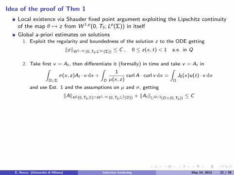
Idea of the proof of Thm 1
Local existence via Shauder fixed point argument exploiting the Lipschitz continuityof the map θ 7rarr z from W 1p(0T0 Lp(Σ)) in itself
Global a-priori estimates on solutions1 Exploit the regularity and boundedness of the solution z to the ODE getting
zW 1infin(0T0Linfin(Σ)) le C 0 le z(x t) lt 1 ae in Q
2 Take first v = At then differentiate it (formally) in time and take v = At inintΩcupΣ
σ(x z)At middot v dx +
intD
1
micro(x z)curlA middot curl v dx =
intΩJ0(x)u(t) middot v dx
and use Est 1 and the assumptions on micro and σ getting
AH1(0T0X)capW 1infin(0T0L2(D)) + AtL103(Dtimes(0T0)) le C
3 Testθt minus∆θ = minusF(θ z)zt + σ(x z)|At |2
by θ and using maximal regularity results for parabolic equations we get
θL2(0T0H1(Σ))capLinfin(0T0L2(Σ))capL53(0T0W 253(Σ))capW 153(0T0L53(Σ)) le C
4 Differentiating (formally) the A-eq and taking v = Att arguing by comparison andusing the results of [Kawanago rsquo93] in order to prove the Linfin-estimate for θ we getthe desired regularity of solutions and we can prolpongate it over the whole timeinterval [0T ]
E Rocca (Universita di Milano) Induction hardening May 14 2013 22 39
Idea of the proof of Thm 1
Local existence via Shauder fixed point argument exploiting the Lipschitz continuityof the map θ 7rarr z from W 1p(0T0 Lp(Σ)) in itself
Global a-priori estimates on solutions1 Exploit the regularity and boundedness of the solution z to the ODE getting
zW 1infin(0T0Linfin(Σ)) le C 0 le z(x t) lt 1 ae in Q
2 Take first v = At then differentiate it (formally) in time and take v = At inintΩcupΣ
σ(x z)At middot v dx +
intD
1
micro(x z)curlA middot curl v dx =
intΩJ0(x)u(t) middot v dx
and use Est 1 and the assumptions on micro and σ getting
AH1(0T0X)capW 1infin(0T0L2(D)) + AtL103(Dtimes(0T0)) le C
3 Testθt minus∆θ = minusF(θ z)zt + σ(x z)|At |2
by θ and using maximal regularity results for parabolic equations we get
θL2(0T0H1(Σ))capLinfin(0T0L2(Σ))capL53(0T0W 253(Σ))capW 153(0T0L53(Σ)) le C
4 Differentiating (formally) the A-eq and taking v = Att arguing by comparison andusing the results of [Kawanago rsquo93] in order to prove the Linfin-estimate for θ we getthe desired regularity of solutions and we can prolpongate it over the whole timeinterval [0T ]
E Rocca (Universita di Milano) Induction hardening May 14 2013 22 39
Idea of the proof of Thm 1
Local existence via Shauder fixed point argument exploiting the Lipschitz continuityof the map θ 7rarr z from W 1p(0T0 Lp(Σ)) in itself
Global a-priori estimates on solutions1 Exploit the regularity and boundedness of the solution z to the ODE getting
zW 1infin(0T0Linfin(Σ)) le C 0 le z(x t) lt 1 ae in Q
2 Take first v = At then differentiate it (formally) in time and take v = At inintΩcupΣ
σ(x z)At middot v dx +
intD
1
micro(x z)curlA middot curl v dx =
intΩJ0(x)u(t) middot v dx
and use Est 1 and the assumptions on micro and σ getting
AH1(0T0X)capW 1infin(0T0L2(D)) + AtL103(Dtimes(0T0)) le C
3 Testθt minus∆θ = minusF(θ z)zt + σ(x z)|At |2
by θ and using maximal regularity results for parabolic equations we get
θL2(0T0H1(Σ))capLinfin(0T0L2(Σ))capL53(0T0W 253(Σ))capW 153(0T0L53(Σ)) le C
4 Differentiating (formally) the A-eq and taking v = Att arguing by comparison andusing the results of [Kawanago rsquo93] in order to prove the Linfin-estimate for θ we getthe desired regularity of solutions and we can prolpongate it over the whole timeinterval [0T ]
E Rocca (Universita di Milano) Induction hardening May 14 2013 22 39
Stability estimate
Differentiate in time equationintΩcupΣ
σ(x z)At middot v dx +
intD
1
micro(x z)curlA middot curl v dx =
intΩ
J0(x)u(t) middot v dx
and take the difference of the two differentiated relations in two solutions (Ai θi zi )and test the difference by (A1 minus A2)t
Use the Lipschitz continuity properties of the solution map to the ODE in z
Take the differences of the equations for θ and test by θ1 minus θ2 exploit the regularityof A and sum up the two relations
E Rocca (Universita di Milano) Induction hardening May 14 2013 23 39
Optimal control problem ndash Existence
cost functional
J (A θ z u) =β1
2
Tint0
intΣ
(θ(x t)minus θd(x t))2dxdt +
β2
2
intΣ
(z(x T )minus zd)2dx +β3
2u2
H1(0T )
control problem (CP)minJ (A θ z u)such that A θ z satisfies (P) and u isin Uad sub H1(0T )
Theorem 2 (CP) has a solution u isin Uad
E Rocca (Universita di Milano) Induction hardening May 14 2013 24 39
Optimal control problem ndash Existence
cost functional
J (A θ z u) =β1
2
Tint0
intΣ
(θ(x t)minus θd(x t))2dxdt +
β2
2
intΣ
(z(x T )minus zd)2dx +β3
2u2
H1(0T )
control problem (CP)minJ (A θ z u)such that A θ z satisfies (P) and u isin Uad sub H1(0T )
Theorem 2 (CP) has a solution u isin Uad
E Rocca (Universita di Milano) Induction hardening May 14 2013 24 39
Optimal control problem ndash Existence
cost functional
J (A θ z u) =β1
2
Tint0
intΣ
(θ(x t)minus θd(x t))2dxdt +
β2
2
intΣ
(z(x T )minus zd)2dx +β3
2u2
H1(0T )
control problem (CP)minJ (A θ z u)such that A θ z satisfies (P) and u isin Uad sub H1(0T )
Theorem 2 (CP) has a solution u isin Uad
E Rocca (Universita di Milano) Induction hardening May 14 2013 24 39
Optimal control problem ndash Differentiability
Lipschitz-continuity the control-to-state mapping
S u 7rarr (A θ z)
is Lipschitz continuous from H1(0T ) to Z by Theorem 1
Frechet differentiability the control-to-state mapping
S u 7rarr (A θ z)
is Frechet differentiable from H1(0T ) to Y Z sub Y
E Rocca (Universita di Milano) Induction hardening May 14 2013 25 39
Optimal control problem ndash First-order necessary conditions of optimality
adjoint systemminusσαt minus curl
( 1
microcurlα
)minus σprime(x z)ztα = minus2(σAtϑ)t
minusϑt minus k∆ϑ+ fθ(θ z)ϑ = fθζ + β1(θ minus θd)
minusζt minus fz(θ z)ζ + σprimeAt middotαminus σprime|At |2ϑ =microprime
micro2curlA middot curlαminus fzϑ
αtimes n = 0 in partD times (0T )
kpartϑ
partν+ κϑ = 0 in partΣtimes (0T )
ϑ(T ) = 0 ζ(T ) = z(x T )minus zd(x) in Σ
α(T ) = 0 in D
variational inequalityTint
0
(β3u(t)minus
intD
α(x t) middot J0(x t)dx)
(u minus u)dt
+
Tint0
β3uprime(t)(uprime(t)minus uprime(t))dt ge 0 for all u isin Uad sub H1(0T )
E Rocca (Universita di Milano) Induction hardening May 14 2013 26 39
Optimal control problem ndash First-order necessary conditions of optimality
adjoint systemminusσαt minus curl
( 1
microcurlα
)minus σprime(x z)ztα = minus2(σAtϑ)t
minusϑt minus k∆ϑ+ fθ(θ z)ϑ = fθζ + β1(θ minus θd)
minusζt minus fz(θ z)ζ + σprimeAt middotαminus σprime|At |2ϑ =microprime
micro2curlA middot curlαminus fzϑ
αtimes n = 0 in partD times (0T )
kpartϑ
partν+ κϑ = 0 in partΣtimes (0T )
ϑ(T ) = 0 ζ(T ) = z(x T )minus zd(x) in Σ
α(T ) = 0 in D
variational inequalityTint
0
(β3u(t)minus
intD
α(x t) middot J0(x t)dx)
(u minus u)dt
+
Tint0
β3uprime(t)(uprime(t)minus uprime(t))dt ge 0 for all u isin Uad sub H1(0T )
E Rocca (Universita di Milano) Induction hardening May 14 2013 26 39
Numerical results ndash Challenges [Homberg Petzold]
Multiple time scalesMagnetic vector potential and heat conductance live on different time scales(Averaging method)
Skin effectEddy currents are distributed in a small surface layer of the workpiece (Adaptivemesh generation)
Nonlinear material dataMagnetic permeability micro depends on temperature and magnetic field H(Linearization)
3DTime consuming simulation in 3D (Model reduction to tackle optimal controlproblem numerically)
E Rocca (Universita di Milano) Induction hardening May 14 2013 27 39
Numerical results ndash Challenges [Homberg Petzold]
Multiple time scalesMagnetic vector potential and heat conductance live on different time scales(Averaging method)
Skin effectEddy currents are distributed in a small surface layer of the workpiece (Adaptivemesh generation)
Nonlinear material dataMagnetic permeability micro depends on temperature and magnetic field H(Linearization)
3DTime consuming simulation in 3D (Model reduction to tackle optimal controlproblem numerically)
E Rocca (Universita di Milano) Induction hardening May 14 2013 27 39
Numerical results ndash Challenges [Homberg Petzold]
Multiple time scalesMagnetic vector potential and heat conductance live on different time scales(Averaging method)
Skin effectEddy currents are distributed in a small surface layer of the workpiece (Adaptivemesh generation)
Nonlinear material dataMagnetic permeability micro depends on temperature and magnetic field H(Linearization)
3DTime consuming simulation in 3D (Model reduction to tackle optimal controlproblem numerically)
E Rocca (Universita di Milano) Induction hardening May 14 2013 27 39
Numerical results ndash Challenges [Homberg Petzold]
Multiple time scalesMagnetic vector potential and heat conductance live on different time scales(Averaging method)
Skin effectEddy currents are distributed in a small surface layer of the workpiece (Adaptivemesh generation)
Nonlinear material dataMagnetic permeability micro depends on temperature and magnetic field H(Linearization)
3DTime consuming simulation in 3D (Model reduction to tackle optimal controlproblem numerically)
E Rocca (Universita di Milano) Induction hardening May 14 2013 27 39
Numerical realization ndash multiple time scales
Time scale for Maxwellrsquos equation governed by frequency of source currentf asymp 10 kHzminus 100 kHz consequetly τ sim 10minus5s
Time scale for heat equation governed by heat diffusion
τ sim cpρL2
kasymp 1 s
Alternating computation
I Solve for A with fixed temperature on fast time-scale
I Compute Joule heat by averaging electric energy Q = 1T
int T0 σ
∣∣∣ partApartt ∣∣∣2 dt
I Solve heat equation with fixed magnetic potential on slow time-scale (one time step)I Update A since σ and micro change with temperature
E Rocca (Universita di Milano) Induction hardening May 14 2013 28 39
Numerical realization ndash multiple time scales
Time scale for Maxwellrsquos equation governed by frequency of source currentf asymp 10 kHzminus 100 kHz consequetly τ sim 10minus5s
Time scale for heat equation governed by heat diffusion
τ sim cpρL2
kasymp 1 s
Alternating computation
I Solve for A with fixed temperature on fast time-scale
I Compute Joule heat by averaging electric energy Q = 1T
int T0 σ
∣∣∣ partApartt ∣∣∣2 dt
I Solve heat equation with fixed magnetic potential on slow time-scale (one time step)I Update A since σ and micro change with temperature
E Rocca (Universita di Milano) Induction hardening May 14 2013 28 39
Thermal and electrical conductivity heat capacity and density
Material data depend on temperature
Electrical conductivity σ(θ)Thermal conductivity κ(θ)
Density ρ(θ)Specific heat capacity cp(θ)
Nonlinear relation between magnetic induction B and magnetic field HMagnetization curve B = micro(θH)H
E Rocca (Universita di Milano) Induction hardening May 14 2013 29 39
Example 1 HF temperature and growth of austenite
(Video austenitemp4)
Figure temperature and austenite growth at high frequency
E Rocca (Universita di Milano) Induction hardening May 14 2013 30 39

Idea of the proof of Thm 1
Local existence via Shauder fixed point argument exploiting the Lipschitz continuityof the map θ 7rarr z from W 1p(0T0 Lp(Σ)) in itself
Global a-priori estimates on solutions1 Exploit the regularity and boundedness of the solution z to the ODE getting
zW 1infin(0T0Linfin(Σ)) le C 0 le z(x t) lt 1 ae in Q
2 Take first v = At then differentiate it (formally) in time and take v = At inintΩcupΣ
σ(x z)At middot v dx +
intD
1
micro(x z)curlA middot curl v dx =
intΩJ0(x)u(t) middot v dx
and use Est 1 and the assumptions on micro and σ getting
AH1(0T0X)capW 1infin(0T0L2(D)) + AtL103(Dtimes(0T0)) le C
3 Testθt minus∆θ = minusF(θ z)zt + σ(x z)|At |2
by θ and using maximal regularity results for parabolic equations we get
θL2(0T0H1(Σ))capLinfin(0T0L2(Σ))capL53(0T0W 253(Σ))capW 153(0T0L53(Σ)) le C
4 Differentiating (formally) the A-eq and taking v = Att arguing by comparison andusing the results of [Kawanago rsquo93] in order to prove the Linfin-estimate for θ we getthe desired regularity of solutions and we can prolpongate it over the whole timeinterval [0T ]
E Rocca (Universita di Milano) Induction hardening May 14 2013 22 39
Idea of the proof of Thm 1
Local existence via Shauder fixed point argument exploiting the Lipschitz continuityof the map θ 7rarr z from W 1p(0T0 Lp(Σ)) in itself
Global a-priori estimates on solutions1 Exploit the regularity and boundedness of the solution z to the ODE getting
zW 1infin(0T0Linfin(Σ)) le C 0 le z(x t) lt 1 ae in Q
2 Take first v = At then differentiate it (formally) in time and take v = At inintΩcupΣ
σ(x z)At middot v dx +
intD
1
micro(x z)curlA middot curl v dx =
intΩJ0(x)u(t) middot v dx
and use Est 1 and the assumptions on micro and σ getting
AH1(0T0X)capW 1infin(0T0L2(D)) + AtL103(Dtimes(0T0)) le C
3 Testθt minus∆θ = minusF(θ z)zt + σ(x z)|At |2
by θ and using maximal regularity results for parabolic equations we get
θL2(0T0H1(Σ))capLinfin(0T0L2(Σ))capL53(0T0W 253(Σ))capW 153(0T0L53(Σ)) le C
4 Differentiating (formally) the A-eq and taking v = Att arguing by comparison andusing the results of [Kawanago rsquo93] in order to prove the Linfin-estimate for θ we getthe desired regularity of solutions and we can prolpongate it over the whole timeinterval [0T ]
E Rocca (Universita di Milano) Induction hardening May 14 2013 22 39
Stability estimate
Differentiate in time equationintΩcupΣ
σ(x z)At middot v dx +
intD
1
micro(x z)curlA middot curl v dx =
intΩ
J0(x)u(t) middot v dx
and take the difference of the two differentiated relations in two solutions (Ai θi zi )and test the difference by (A1 minus A2)t
Use the Lipschitz continuity properties of the solution map to the ODE in z
Take the differences of the equations for θ and test by θ1 minus θ2 exploit the regularityof A and sum up the two relations
E Rocca (Universita di Milano) Induction hardening May 14 2013 23 39
Optimal control problem ndash Existence
cost functional
J (A θ z u) =β1
2
Tint0
intΣ
(θ(x t)minus θd(x t))2dxdt +
β2
2
intΣ
(z(x T )minus zd)2dx +β3
2u2
H1(0T )
control problem (CP)minJ (A θ z u)such that A θ z satisfies (P) and u isin Uad sub H1(0T )
Theorem 2 (CP) has a solution u isin Uad
E Rocca (Universita di Milano) Induction hardening May 14 2013 24 39
Optimal control problem ndash Existence
cost functional
J (A θ z u) =β1
2
Tint0
intΣ
(θ(x t)minus θd(x t))2dxdt +
β2
2
intΣ
(z(x T )minus zd)2dx +β3
2u2
H1(0T )
control problem (CP)minJ (A θ z u)such that A θ z satisfies (P) and u isin Uad sub H1(0T )
Theorem 2 (CP) has a solution u isin Uad
E Rocca (Universita di Milano) Induction hardening May 14 2013 24 39
Optimal control problem ndash Existence
cost functional
J (A θ z u) =β1
2
Tint0
intΣ
(θ(x t)minus θd(x t))2dxdt +
β2
2
intΣ
(z(x T )minus zd)2dx +β3
2u2
H1(0T )
control problem (CP)minJ (A θ z u)such that A θ z satisfies (P) and u isin Uad sub H1(0T )
Theorem 2 (CP) has a solution u isin Uad
E Rocca (Universita di Milano) Induction hardening May 14 2013 24 39
Optimal control problem ndash Differentiability
Lipschitz-continuity the control-to-state mapping
S u 7rarr (A θ z)
is Lipschitz continuous from H1(0T ) to Z by Theorem 1
Frechet differentiability the control-to-state mapping
S u 7rarr (A θ z)
is Frechet differentiable from H1(0T ) to Y Z sub Y
E Rocca (Universita di Milano) Induction hardening May 14 2013 25 39
Optimal control problem ndash First-order necessary conditions of optimality
adjoint systemminusσαt minus curl
( 1
microcurlα
)minus σprime(x z)ztα = minus2(σAtϑ)t
minusϑt minus k∆ϑ+ fθ(θ z)ϑ = fθζ + β1(θ minus θd)
minusζt minus fz(θ z)ζ + σprimeAt middotαminus σprime|At |2ϑ =microprime
micro2curlA middot curlαminus fzϑ
αtimes n = 0 in partD times (0T )
kpartϑ
partν+ κϑ = 0 in partΣtimes (0T )
ϑ(T ) = 0 ζ(T ) = z(x T )minus zd(x) in Σ
α(T ) = 0 in D
variational inequalityTint
0
(β3u(t)minus
intD
α(x t) middot J0(x t)dx)
(u minus u)dt
+
Tint0
β3uprime(t)(uprime(t)minus uprime(t))dt ge 0 for all u isin Uad sub H1(0T )
E Rocca (Universita di Milano) Induction hardening May 14 2013 26 39
Optimal control problem ndash First-order necessary conditions of optimality
adjoint systemminusσαt minus curl
( 1
microcurlα
)minus σprime(x z)ztα = minus2(σAtϑ)t
minusϑt minus k∆ϑ+ fθ(θ z)ϑ = fθζ + β1(θ minus θd)
minusζt minus fz(θ z)ζ + σprimeAt middotαminus σprime|At |2ϑ =microprime
micro2curlA middot curlαminus fzϑ
αtimes n = 0 in partD times (0T )
kpartϑ
partν+ κϑ = 0 in partΣtimes (0T )
ϑ(T ) = 0 ζ(T ) = z(x T )minus zd(x) in Σ
α(T ) = 0 in D
variational inequalityTint
0
(β3u(t)minus
intD
α(x t) middot J0(x t)dx)
(u minus u)dt
+
Tint0
β3uprime(t)(uprime(t)minus uprime(t))dt ge 0 for all u isin Uad sub H1(0T )
E Rocca (Universita di Milano) Induction hardening May 14 2013 26 39
Numerical results ndash Challenges [Homberg Petzold]
Multiple time scalesMagnetic vector potential and heat conductance live on different time scales(Averaging method)
Skin effectEddy currents are distributed in a small surface layer of the workpiece (Adaptivemesh generation)
Nonlinear material dataMagnetic permeability micro depends on temperature and magnetic field H(Linearization)
3DTime consuming simulation in 3D (Model reduction to tackle optimal controlproblem numerically)
E Rocca (Universita di Milano) Induction hardening May 14 2013 27 39
Numerical results ndash Challenges [Homberg Petzold]
Multiple time scalesMagnetic vector potential and heat conductance live on different time scales(Averaging method)
Skin effectEddy currents are distributed in a small surface layer of the workpiece (Adaptivemesh generation)
Nonlinear material dataMagnetic permeability micro depends on temperature and magnetic field H(Linearization)
3DTime consuming simulation in 3D (Model reduction to tackle optimal controlproblem numerically)
E Rocca (Universita di Milano) Induction hardening May 14 2013 27 39
Numerical results ndash Challenges [Homberg Petzold]
Multiple time scalesMagnetic vector potential and heat conductance live on different time scales(Averaging method)
Skin effectEddy currents are distributed in a small surface layer of the workpiece (Adaptivemesh generation)
Nonlinear material dataMagnetic permeability micro depends on temperature and magnetic field H(Linearization)
3DTime consuming simulation in 3D (Model reduction to tackle optimal controlproblem numerically)
E Rocca (Universita di Milano) Induction hardening May 14 2013 27 39
Numerical results ndash Challenges [Homberg Petzold]
Multiple time scalesMagnetic vector potential and heat conductance live on different time scales(Averaging method)
Skin effectEddy currents are distributed in a small surface layer of the workpiece (Adaptivemesh generation)
Nonlinear material dataMagnetic permeability micro depends on temperature and magnetic field H(Linearization)
3DTime consuming simulation in 3D (Model reduction to tackle optimal controlproblem numerically)
E Rocca (Universita di Milano) Induction hardening May 14 2013 27 39
Numerical realization ndash multiple time scales
Time scale for Maxwellrsquos equation governed by frequency of source currentf asymp 10 kHzminus 100 kHz consequetly τ sim 10minus5s
Time scale for heat equation governed by heat diffusion
τ sim cpρL2
kasymp 1 s
Alternating computation
I Solve for A with fixed temperature on fast time-scale
I Compute Joule heat by averaging electric energy Q = 1T
int T0 σ
∣∣∣ partApartt ∣∣∣2 dt
I Solve heat equation with fixed magnetic potential on slow time-scale (one time step)I Update A since σ and micro change with temperature
E Rocca (Universita di Milano) Induction hardening May 14 2013 28 39
Numerical realization ndash multiple time scales
Time scale for Maxwellrsquos equation governed by frequency of source currentf asymp 10 kHzminus 100 kHz consequetly τ sim 10minus5s
Time scale for heat equation governed by heat diffusion
τ sim cpρL2
kasymp 1 s
Alternating computation
I Solve for A with fixed temperature on fast time-scale
I Compute Joule heat by averaging electric energy Q = 1T
int T0 σ
∣∣∣ partApartt ∣∣∣2 dt
I Solve heat equation with fixed magnetic potential on slow time-scale (one time step)I Update A since σ and micro change with temperature
E Rocca (Universita di Milano) Induction hardening May 14 2013 28 39
Thermal and electrical conductivity heat capacity and density
Material data depend on temperature
Electrical conductivity σ(θ)Thermal conductivity κ(θ)
Density ρ(θ)Specific heat capacity cp(θ)
Nonlinear relation between magnetic induction B and magnetic field HMagnetization curve B = micro(θH)H
E Rocca (Universita di Milano) Induction hardening May 14 2013 29 39
Example 1 HF temperature and growth of austenite
(Video austenitemp4)
Figure temperature and austenite growth at high frequency
E Rocca (Universita di Milano) Induction hardening May 14 2013 30 39

Idea of the proof of Thm 1
Local existence via Shauder fixed point argument exploiting the Lipschitz continuityof the map θ 7rarr z from W 1p(0T0 Lp(Σ)) in itself
Global a-priori estimates on solutions1 Exploit the regularity and boundedness of the solution z to the ODE getting
zW 1infin(0T0Linfin(Σ)) le C 0 le z(x t) lt 1 ae in Q
2 Take first v = At then differentiate it (formally) in time and take v = At inintΩcupΣ
σ(x z)At middot v dx +
intD
1
micro(x z)curlA middot curl v dx =
intΩJ0(x)u(t) middot v dx
and use Est 1 and the assumptions on micro and σ getting
AH1(0T0X)capW 1infin(0T0L2(D)) + AtL103(Dtimes(0T0)) le C
3 Testθt minus∆θ = minusF(θ z)zt + σ(x z)|At |2
by θ and using maximal regularity results for parabolic equations we get
θL2(0T0H1(Σ))capLinfin(0T0L2(Σ))capL53(0T0W 253(Σ))capW 153(0T0L53(Σ)) le C
4 Differentiating (formally) the A-eq and taking v = Att arguing by comparison andusing the results of [Kawanago rsquo93] in order to prove the Linfin-estimate for θ we getthe desired regularity of solutions and we can prolpongate it over the whole timeinterval [0T ]
E Rocca (Universita di Milano) Induction hardening May 14 2013 22 39
Stability estimate
Differentiate in time equationintΩcupΣ
σ(x z)At middot v dx +
intD
1
micro(x z)curlA middot curl v dx =
intΩ
J0(x)u(t) middot v dx
and take the difference of the two differentiated relations in two solutions (Ai θi zi )and test the difference by (A1 minus A2)t
Use the Lipschitz continuity properties of the solution map to the ODE in z
Take the differences of the equations for θ and test by θ1 minus θ2 exploit the regularityof A and sum up the two relations
E Rocca (Universita di Milano) Induction hardening May 14 2013 23 39
Optimal control problem ndash Existence
cost functional
J (A θ z u) =β1
2
Tint0
intΣ
(θ(x t)minus θd(x t))2dxdt +
β2
2
intΣ
(z(x T )minus zd)2dx +β3
2u2
H1(0T )
control problem (CP)minJ (A θ z u)such that A θ z satisfies (P) and u isin Uad sub H1(0T )
Theorem 2 (CP) has a solution u isin Uad
E Rocca (Universita di Milano) Induction hardening May 14 2013 24 39
Optimal control problem ndash Existence
cost functional
J (A θ z u) =β1
2
Tint0
intΣ
(θ(x t)minus θd(x t))2dxdt +
β2
2
intΣ
(z(x T )minus zd)2dx +β3
2u2
H1(0T )
control problem (CP)minJ (A θ z u)such that A θ z satisfies (P) and u isin Uad sub H1(0T )
Theorem 2 (CP) has a solution u isin Uad
E Rocca (Universita di Milano) Induction hardening May 14 2013 24 39
Optimal control problem ndash Existence
cost functional
J (A θ z u) =β1
2
Tint0
intΣ
(θ(x t)minus θd(x t))2dxdt +
β2
2
intΣ
(z(x T )minus zd)2dx +β3
2u2
H1(0T )
control problem (CP)minJ (A θ z u)such that A θ z satisfies (P) and u isin Uad sub H1(0T )
Theorem 2 (CP) has a solution u isin Uad
E Rocca (Universita di Milano) Induction hardening May 14 2013 24 39
Optimal control problem ndash Differentiability
Lipschitz-continuity the control-to-state mapping
S u 7rarr (A θ z)
is Lipschitz continuous from H1(0T ) to Z by Theorem 1
Frechet differentiability the control-to-state mapping
S u 7rarr (A θ z)
is Frechet differentiable from H1(0T ) to Y Z sub Y
E Rocca (Universita di Milano) Induction hardening May 14 2013 25 39
Optimal control problem ndash First-order necessary conditions of optimality
adjoint systemminusσαt minus curl
( 1
microcurlα
)minus σprime(x z)ztα = minus2(σAtϑ)t
minusϑt minus k∆ϑ+ fθ(θ z)ϑ = fθζ + β1(θ minus θd)
minusζt minus fz(θ z)ζ + σprimeAt middotαminus σprime|At |2ϑ =microprime
micro2curlA middot curlαminus fzϑ
αtimes n = 0 in partD times (0T )
kpartϑ
partν+ κϑ = 0 in partΣtimes (0T )
ϑ(T ) = 0 ζ(T ) = z(x T )minus zd(x) in Σ
α(T ) = 0 in D
variational inequalityTint
0
(β3u(t)minus
intD
α(x t) middot J0(x t)dx)
(u minus u)dt
+
Tint0
β3uprime(t)(uprime(t)minus uprime(t))dt ge 0 for all u isin Uad sub H1(0T )
E Rocca (Universita di Milano) Induction hardening May 14 2013 26 39
Optimal control problem ndash First-order necessary conditions of optimality
adjoint systemminusσαt minus curl
( 1
microcurlα
)minus σprime(x z)ztα = minus2(σAtϑ)t
minusϑt minus k∆ϑ+ fθ(θ z)ϑ = fθζ + β1(θ minus θd)
minusζt minus fz(θ z)ζ + σprimeAt middotαminus σprime|At |2ϑ =microprime
micro2curlA middot curlαminus fzϑ
αtimes n = 0 in partD times (0T )
kpartϑ
partν+ κϑ = 0 in partΣtimes (0T )
ϑ(T ) = 0 ζ(T ) = z(x T )minus zd(x) in Σ
α(T ) = 0 in D
variational inequalityTint
0
(β3u(t)minus
intD
α(x t) middot J0(x t)dx)
(u minus u)dt
+
Tint0
β3uprime(t)(uprime(t)minus uprime(t))dt ge 0 for all u isin Uad sub H1(0T )
E Rocca (Universita di Milano) Induction hardening May 14 2013 26 39
Numerical results ndash Challenges [Homberg Petzold]
Multiple time scalesMagnetic vector potential and heat conductance live on different time scales(Averaging method)
Skin effectEddy currents are distributed in a small surface layer of the workpiece (Adaptivemesh generation)
Nonlinear material dataMagnetic permeability micro depends on temperature and magnetic field H(Linearization)
3DTime consuming simulation in 3D (Model reduction to tackle optimal controlproblem numerically)
E Rocca (Universita di Milano) Induction hardening May 14 2013 27 39
Numerical results ndash Challenges [Homberg Petzold]
Multiple time scalesMagnetic vector potential and heat conductance live on different time scales(Averaging method)
Skin effectEddy currents are distributed in a small surface layer of the workpiece (Adaptivemesh generation)
Nonlinear material dataMagnetic permeability micro depends on temperature and magnetic field H(Linearization)
3DTime consuming simulation in 3D (Model reduction to tackle optimal controlproblem numerically)
E Rocca (Universita di Milano) Induction hardening May 14 2013 27 39
Numerical results ndash Challenges [Homberg Petzold]
Multiple time scalesMagnetic vector potential and heat conductance live on different time scales(Averaging method)
Skin effectEddy currents are distributed in a small surface layer of the workpiece (Adaptivemesh generation)
Nonlinear material dataMagnetic permeability micro depends on temperature and magnetic field H(Linearization)
3DTime consuming simulation in 3D (Model reduction to tackle optimal controlproblem numerically)
E Rocca (Universita di Milano) Induction hardening May 14 2013 27 39
Numerical results ndash Challenges [Homberg Petzold]
Multiple time scalesMagnetic vector potential and heat conductance live on different time scales(Averaging method)
Skin effectEddy currents are distributed in a small surface layer of the workpiece (Adaptivemesh generation)
Nonlinear material dataMagnetic permeability micro depends on temperature and magnetic field H(Linearization)
3DTime consuming simulation in 3D (Model reduction to tackle optimal controlproblem numerically)
E Rocca (Universita di Milano) Induction hardening May 14 2013 27 39
Numerical realization ndash multiple time scales
Time scale for Maxwellrsquos equation governed by frequency of source currentf asymp 10 kHzminus 100 kHz consequetly τ sim 10minus5s
Time scale for heat equation governed by heat diffusion
τ sim cpρL2
kasymp 1 s
Alternating computation
I Solve for A with fixed temperature on fast time-scale
I Compute Joule heat by averaging electric energy Q = 1T
int T0 σ
∣∣∣ partApartt ∣∣∣2 dt
I Solve heat equation with fixed magnetic potential on slow time-scale (one time step)I Update A since σ and micro change with temperature
E Rocca (Universita di Milano) Induction hardening May 14 2013 28 39
Numerical realization ndash multiple time scales
Time scale for Maxwellrsquos equation governed by frequency of source currentf asymp 10 kHzminus 100 kHz consequetly τ sim 10minus5s
Time scale for heat equation governed by heat diffusion
τ sim cpρL2
kasymp 1 s
Alternating computation
I Solve for A with fixed temperature on fast time-scale
I Compute Joule heat by averaging electric energy Q = 1T
int T0 σ
∣∣∣ partApartt ∣∣∣2 dt
I Solve heat equation with fixed magnetic potential on slow time-scale (one time step)I Update A since σ and micro change with temperature
E Rocca (Universita di Milano) Induction hardening May 14 2013 28 39
Thermal and electrical conductivity heat capacity and density
Material data depend on temperature
Electrical conductivity σ(θ)Thermal conductivity κ(θ)
Density ρ(θ)Specific heat capacity cp(θ)
Nonlinear relation between magnetic induction B and magnetic field HMagnetization curve B = micro(θH)H
E Rocca (Universita di Milano) Induction hardening May 14 2013 29 39
Example 1 HF temperature and growth of austenite
(Video austenitemp4)
Figure temperature and austenite growth at high frequency
E Rocca (Universita di Milano) Induction hardening May 14 2013 30 39

Optimal control problem ndash Existence
cost functional
J (A θ z u) =β1
2
Tint0
intΣ
(θ(x t)minus θd(x t))2dxdt +
β2
2
intΣ
(z(x T )minus zd)2dx +β3
2u2
H1(0T )
control problem (CP)minJ (A θ z u)such that A θ z satisfies (P) and u isin Uad sub H1(0T )
Theorem 2 (CP) has a solution u isin Uad
E Rocca (Universita di Milano) Induction hardening May 14 2013 24 39
Optimal control problem ndash Differentiability
Lipschitz-continuity the control-to-state mapping
S u 7rarr (A θ z)
is Lipschitz continuous from H1(0T ) to Z by Theorem 1
Frechet differentiability the control-to-state mapping
S u 7rarr (A θ z)
is Frechet differentiable from H1(0T ) to Y Z sub Y
E Rocca (Universita di Milano) Induction hardening May 14 2013 25 39
Optimal control problem ndash First-order necessary conditions of optimality
adjoint systemminusσαt minus curl
( 1
microcurlα
)minus σprime(x z)ztα = minus2(σAtϑ)t
minusϑt minus k∆ϑ+ fθ(θ z)ϑ = fθζ + β1(θ minus θd)
minusζt minus fz(θ z)ζ + σprimeAt middotαminus σprime|At |2ϑ =microprime
micro2curlA middot curlαminus fzϑ
αtimes n = 0 in partD times (0T )
kpartϑ
partν+ κϑ = 0 in partΣtimes (0T )
ϑ(T ) = 0 ζ(T ) = z(x T )minus zd(x) in Σ
α(T ) = 0 in D
variational inequalityTint
0
(β3u(t)minus
intD
α(x t) middot J0(x t)dx)
(u minus u)dt
+
Tint0
β3uprime(t)(uprime(t)minus uprime(t))dt ge 0 for all u isin Uad sub H1(0T )
E Rocca (Universita di Milano) Induction hardening May 14 2013 26 39
Optimal control problem ndash First-order necessary conditions of optimality
adjoint systemminusσαt minus curl
( 1
microcurlα
)minus σprime(x z)ztα = minus2(σAtϑ)t
minusϑt minus k∆ϑ+ fθ(θ z)ϑ = fθζ + β1(θ minus θd)
minusζt minus fz(θ z)ζ + σprimeAt middotαminus σprime|At |2ϑ =microprime
micro2curlA middot curlαminus fzϑ
αtimes n = 0 in partD times (0T )
kpartϑ
partν+ κϑ = 0 in partΣtimes (0T )
ϑ(T ) = 0 ζ(T ) = z(x T )minus zd(x) in Σ
α(T ) = 0 in D
variational inequalityTint
0
(β3u(t)minus
intD
α(x t) middot J0(x t)dx)
(u minus u)dt
+
Tint0
β3uprime(t)(uprime(t)minus uprime(t))dt ge 0 for all u isin Uad sub H1(0T )
E Rocca (Universita di Milano) Induction hardening May 14 2013 26 39
Numerical results ndash Challenges [Homberg Petzold]
Multiple time scalesMagnetic vector potential and heat conductance live on different time scales(Averaging method)
Skin effectEddy currents are distributed in a small surface layer of the workpiece (Adaptivemesh generation)
Nonlinear material dataMagnetic permeability micro depends on temperature and magnetic field H(Linearization)
3DTime consuming simulation in 3D (Model reduction to tackle optimal controlproblem numerically)
E Rocca (Universita di Milano) Induction hardening May 14 2013 27 39
Numerical results ndash Challenges [Homberg Petzold]
Multiple time scalesMagnetic vector potential and heat conductance live on different time scales(Averaging method)
Skin effectEddy currents are distributed in a small surface layer of the workpiece (Adaptivemesh generation)
Nonlinear material dataMagnetic permeability micro depends on temperature and magnetic field H(Linearization)
3DTime consuming simulation in 3D (Model reduction to tackle optimal controlproblem numerically)
E Rocca (Universita di Milano) Induction hardening May 14 2013 27 39
Numerical results ndash Challenges [Homberg Petzold]
Multiple time scalesMagnetic vector potential and heat conductance live on different time scales(Averaging method)
Skin effectEddy currents are distributed in a small surface layer of the workpiece (Adaptivemesh generation)
Nonlinear material dataMagnetic permeability micro depends on temperature and magnetic field H(Linearization)
3DTime consuming simulation in 3D (Model reduction to tackle optimal controlproblem numerically)
E Rocca (Universita di Milano) Induction hardening May 14 2013 27 39
Numerical results ndash Challenges [Homberg Petzold]
Multiple time scalesMagnetic vector potential and heat conductance live on different time scales(Averaging method)
Skin effectEddy currents are distributed in a small surface layer of the workpiece (Adaptivemesh generation)
Nonlinear material dataMagnetic permeability micro depends on temperature and magnetic field H(Linearization)
3DTime consuming simulation in 3D (Model reduction to tackle optimal controlproblem numerically)
E Rocca (Universita di Milano) Induction hardening May 14 2013 27 39
Numerical realization ndash multiple time scales
Time scale for Maxwellrsquos equation governed by frequency of source currentf asymp 10 kHzminus 100 kHz consequetly τ sim 10minus5s
Time scale for heat equation governed by heat diffusion
τ sim cpρL2
kasymp 1 s
Alternating computation
I Solve for A with fixed temperature on fast time-scale
I Compute Joule heat by averaging electric energy Q = 1T
int T0 σ
∣∣∣ partApartt ∣∣∣2 dt
I Solve heat equation with fixed magnetic potential on slow time-scale (one time step)I Update A since σ and micro change with temperature
E Rocca (Universita di Milano) Induction hardening May 14 2013 28 39
Numerical realization ndash multiple time scales
Time scale for Maxwellrsquos equation governed by frequency of source currentf asymp 10 kHzminus 100 kHz consequetly τ sim 10minus5s
Time scale for heat equation governed by heat diffusion
τ sim cpρL2
kasymp 1 s
Alternating computation
I Solve for A with fixed temperature on fast time-scale
I Compute Joule heat by averaging electric energy Q = 1T
int T0 σ
∣∣∣ partApartt ∣∣∣2 dt
I Solve heat equation with fixed magnetic potential on slow time-scale (one time step)I Update A since σ and micro change with temperature
E Rocca (Universita di Milano) Induction hardening May 14 2013 28 39
Thermal and electrical conductivity heat capacity and density
Material data depend on temperature
Electrical conductivity σ(θ)Thermal conductivity κ(θ)
Density ρ(θ)Specific heat capacity cp(θ)
Nonlinear relation between magnetic induction B and magnetic field HMagnetization curve B = micro(θH)H
E Rocca (Universita di Milano) Induction hardening May 14 2013 29 39
Example 1 HF temperature and growth of austenite
(Video austenitemp4)
Figure temperature and austenite growth at high frequency
E Rocca (Universita di Milano) Induction hardening May 14 2013 30 39

Optimal control problem ndash Existence
cost functional
J (A θ z u) =β1
2
Tint0
intΣ
(θ(x t)minus θd(x t))2dxdt +
β2
2
intΣ
(z(x T )minus zd)2dx +β3
2u2
H1(0T )
control problem (CP)minJ (A θ z u)such that A θ z satisfies (P) and u isin Uad sub H1(0T )
Theorem 2 (CP) has a solution u isin Uad
E Rocca (Universita di Milano) Induction hardening May 14 2013 24 39
Optimal control problem ndash Existence
cost functional
J (A θ z u) =β1
2
Tint0
intΣ
(θ(x t)minus θd(x t))2dxdt +
β2
2
intΣ
(z(x T )minus zd)2dx +β3
2u2
H1(0T )
control problem (CP)minJ (A θ z u)such that A θ z satisfies (P) and u isin Uad sub H1(0T )
Theorem 2 (CP) has a solution u isin Uad
E Rocca (Universita di Milano) Induction hardening May 14 2013 24 39
Optimal control problem ndash Differentiability
Lipschitz-continuity the control-to-state mapping
S u 7rarr (A θ z)
is Lipschitz continuous from H1(0T ) to Z by Theorem 1
Frechet differentiability the control-to-state mapping
S u 7rarr (A θ z)
is Frechet differentiable from H1(0T ) to Y Z sub Y
E Rocca (Universita di Milano) Induction hardening May 14 2013 25 39
Optimal control problem ndash First-order necessary conditions of optimality
adjoint systemminusσαt minus curl
( 1
microcurlα
)minus σprime(x z)ztα = minus2(σAtϑ)t
minusϑt minus k∆ϑ+ fθ(θ z)ϑ = fθζ + β1(θ minus θd)
minusζt minus fz(θ z)ζ + σprimeAt middotαminus σprime|At |2ϑ =microprime
micro2curlA middot curlαminus fzϑ
αtimes n = 0 in partD times (0T )
kpartϑ
partν+ κϑ = 0 in partΣtimes (0T )
ϑ(T ) = 0 ζ(T ) = z(x T )minus zd(x) in Σ
α(T ) = 0 in D
variational inequalityTint
0
(β3u(t)minus
intD
α(x t) middot J0(x t)dx)
(u minus u)dt
+
Tint0
β3uprime(t)(uprime(t)minus uprime(t))dt ge 0 for all u isin Uad sub H1(0T )
E Rocca (Universita di Milano) Induction hardening May 14 2013 26 39
Optimal control problem ndash First-order necessary conditions of optimality
adjoint systemminusσαt minus curl
( 1
microcurlα
)minus σprime(x z)ztα = minus2(σAtϑ)t
minusϑt minus k∆ϑ+ fθ(θ z)ϑ = fθζ + β1(θ minus θd)
minusζt minus fz(θ z)ζ + σprimeAt middotαminus σprime|At |2ϑ =microprime
micro2curlA middot curlαminus fzϑ
αtimes n = 0 in partD times (0T )
kpartϑ
partν+ κϑ = 0 in partΣtimes (0T )
ϑ(T ) = 0 ζ(T ) = z(x T )minus zd(x) in Σ
α(T ) = 0 in D
variational inequalityTint
0
(β3u(t)minus
intD
α(x t) middot J0(x t)dx)
(u minus u)dt
+
Tint0
β3uprime(t)(uprime(t)minus uprime(t))dt ge 0 for all u isin Uad sub H1(0T )
E Rocca (Universita di Milano) Induction hardening May 14 2013 26 39
Numerical results ndash Challenges [Homberg Petzold]
Multiple time scalesMagnetic vector potential and heat conductance live on different time scales(Averaging method)
Skin effectEddy currents are distributed in a small surface layer of the workpiece (Adaptivemesh generation)
Nonlinear material dataMagnetic permeability micro depends on temperature and magnetic field H(Linearization)
3DTime consuming simulation in 3D (Model reduction to tackle optimal controlproblem numerically)
E Rocca (Universita di Milano) Induction hardening May 14 2013 27 39
Numerical results ndash Challenges [Homberg Petzold]
Multiple time scalesMagnetic vector potential and heat conductance live on different time scales(Averaging method)
Skin effectEddy currents are distributed in a small surface layer of the workpiece (Adaptivemesh generation)
Nonlinear material dataMagnetic permeability micro depends on temperature and magnetic field H(Linearization)
3DTime consuming simulation in 3D (Model reduction to tackle optimal controlproblem numerically)
E Rocca (Universita di Milano) Induction hardening May 14 2013 27 39
Numerical results ndash Challenges [Homberg Petzold]
Multiple time scalesMagnetic vector potential and heat conductance live on different time scales(Averaging method)
Skin effectEddy currents are distributed in a small surface layer of the workpiece (Adaptivemesh generation)
Nonlinear material dataMagnetic permeability micro depends on temperature and magnetic field H(Linearization)
3DTime consuming simulation in 3D (Model reduction to tackle optimal controlproblem numerically)
E Rocca (Universita di Milano) Induction hardening May 14 2013 27 39
Numerical results ndash Challenges [Homberg Petzold]
Multiple time scalesMagnetic vector potential and heat conductance live on different time scales(Averaging method)
Skin effectEddy currents are distributed in a small surface layer of the workpiece (Adaptivemesh generation)
Nonlinear material dataMagnetic permeability micro depends on temperature and magnetic field H(Linearization)
3DTime consuming simulation in 3D (Model reduction to tackle optimal controlproblem numerically)
E Rocca (Universita di Milano) Induction hardening May 14 2013 27 39
Numerical realization ndash multiple time scales
Time scale for Maxwellrsquos equation governed by frequency of source currentf asymp 10 kHzminus 100 kHz consequetly τ sim 10minus5s
Time scale for heat equation governed by heat diffusion
τ sim cpρL2
kasymp 1 s
Alternating computation
I Solve for A with fixed temperature on fast time-scale
I Compute Joule heat by averaging electric energy Q = 1T
int T0 σ
∣∣∣ partApartt ∣∣∣2 dt
I Solve heat equation with fixed magnetic potential on slow time-scale (one time step)I Update A since σ and micro change with temperature
E Rocca (Universita di Milano) Induction hardening May 14 2013 28 39
Numerical realization ndash multiple time scales
Time scale for Maxwellrsquos equation governed by frequency of source currentf asymp 10 kHzminus 100 kHz consequetly τ sim 10minus5s
Time scale for heat equation governed by heat diffusion
τ sim cpρL2
kasymp 1 s
Alternating computation
I Solve for A with fixed temperature on fast time-scale
I Compute Joule heat by averaging electric energy Q = 1T
int T0 σ
∣∣∣ partApartt ∣∣∣2 dt
I Solve heat equation with fixed magnetic potential on slow time-scale (one time step)I Update A since σ and micro change with temperature
E Rocca (Universita di Milano) Induction hardening May 14 2013 28 39
Thermal and electrical conductivity heat capacity and density
Material data depend on temperature
Electrical conductivity σ(θ)Thermal conductivity κ(θ)
Density ρ(θ)Specific heat capacity cp(θ)
Nonlinear relation between magnetic induction B and magnetic field HMagnetization curve B = micro(θH)H
E Rocca (Universita di Milano) Induction hardening May 14 2013 29 39
Example 1 HF temperature and growth of austenite
(Video austenitemp4)
Figure temperature and austenite growth at high frequency
E Rocca (Universita di Milano) Induction hardening May 14 2013 30 39

Optimal control problem ndash Existence
cost functional
J (A θ z u) =β1
2
Tint0
intΣ
(θ(x t)minus θd(x t))2dxdt +
β2
2
intΣ
(z(x T )minus zd)2dx +β3
2u2
H1(0T )
control problem (CP)minJ (A θ z u)such that A θ z satisfies (P) and u isin Uad sub H1(0T )
Theorem 2 (CP) has a solution u isin Uad
E Rocca (Universita di Milano) Induction hardening May 14 2013 24 39
Optimal control problem ndash Differentiability
Lipschitz-continuity the control-to-state mapping
S u 7rarr (A θ z)
is Lipschitz continuous from H1(0T ) to Z by Theorem 1
Frechet differentiability the control-to-state mapping
S u 7rarr (A θ z)
is Frechet differentiable from H1(0T ) to Y Z sub Y
E Rocca (Universita di Milano) Induction hardening May 14 2013 25 39
Optimal control problem ndash First-order necessary conditions of optimality
adjoint systemminusσαt minus curl
( 1
microcurlα
)minus σprime(x z)ztα = minus2(σAtϑ)t
minusϑt minus k∆ϑ+ fθ(θ z)ϑ = fθζ + β1(θ minus θd)
minusζt minus fz(θ z)ζ + σprimeAt middotαminus σprime|At |2ϑ =microprime
micro2curlA middot curlαminus fzϑ
αtimes n = 0 in partD times (0T )
kpartϑ
partν+ κϑ = 0 in partΣtimes (0T )
ϑ(T ) = 0 ζ(T ) = z(x T )minus zd(x) in Σ
α(T ) = 0 in D
variational inequalityTint
0
(β3u(t)minus
intD
α(x t) middot J0(x t)dx)
(u minus u)dt
+
Tint0
β3uprime(t)(uprime(t)minus uprime(t))dt ge 0 for all u isin Uad sub H1(0T )
E Rocca (Universita di Milano) Induction hardening May 14 2013 26 39
Optimal control problem ndash First-order necessary conditions of optimality
adjoint systemminusσαt minus curl
( 1
microcurlα
)minus σprime(x z)ztα = minus2(σAtϑ)t
minusϑt minus k∆ϑ+ fθ(θ z)ϑ = fθζ + β1(θ minus θd)
minusζt minus fz(θ z)ζ + σprimeAt middotαminus σprime|At |2ϑ =microprime
micro2curlA middot curlαminus fzϑ
αtimes n = 0 in partD times (0T )
kpartϑ
partν+ κϑ = 0 in partΣtimes (0T )
ϑ(T ) = 0 ζ(T ) = z(x T )minus zd(x) in Σ
α(T ) = 0 in D
variational inequalityTint
0
(β3u(t)minus
intD
α(x t) middot J0(x t)dx)
(u minus u)dt
+
Tint0
β3uprime(t)(uprime(t)minus uprime(t))dt ge 0 for all u isin Uad sub H1(0T )
E Rocca (Universita di Milano) Induction hardening May 14 2013 26 39
Numerical results ndash Challenges [Homberg Petzold]
Multiple time scalesMagnetic vector potential and heat conductance live on different time scales(Averaging method)
Skin effectEddy currents are distributed in a small surface layer of the workpiece (Adaptivemesh generation)
Nonlinear material dataMagnetic permeability micro depends on temperature and magnetic field H(Linearization)
3DTime consuming simulation in 3D (Model reduction to tackle optimal controlproblem numerically)
E Rocca (Universita di Milano) Induction hardening May 14 2013 27 39
Numerical results ndash Challenges [Homberg Petzold]
Multiple time scalesMagnetic vector potential and heat conductance live on different time scales(Averaging method)
Skin effectEddy currents are distributed in a small surface layer of the workpiece (Adaptivemesh generation)
Nonlinear material dataMagnetic permeability micro depends on temperature and magnetic field H(Linearization)
3DTime consuming simulation in 3D (Model reduction to tackle optimal controlproblem numerically)
E Rocca (Universita di Milano) Induction hardening May 14 2013 27 39
Numerical results ndash Challenges [Homberg Petzold]
Multiple time scalesMagnetic vector potential and heat conductance live on different time scales(Averaging method)
Skin effectEddy currents are distributed in a small surface layer of the workpiece (Adaptivemesh generation)
Nonlinear material dataMagnetic permeability micro depends on temperature and magnetic field H(Linearization)
3DTime consuming simulation in 3D (Model reduction to tackle optimal controlproblem numerically)
E Rocca (Universita di Milano) Induction hardening May 14 2013 27 39
Numerical results ndash Challenges [Homberg Petzold]
Multiple time scalesMagnetic vector potential and heat conductance live on different time scales(Averaging method)
Skin effectEddy currents are distributed in a small surface layer of the workpiece (Adaptivemesh generation)
Nonlinear material dataMagnetic permeability micro depends on temperature and magnetic field H(Linearization)
3DTime consuming simulation in 3D (Model reduction to tackle optimal controlproblem numerically)
E Rocca (Universita di Milano) Induction hardening May 14 2013 27 39
Numerical realization ndash multiple time scales
Time scale for Maxwellrsquos equation governed by frequency of source currentf asymp 10 kHzminus 100 kHz consequetly τ sim 10minus5s
Time scale for heat equation governed by heat diffusion
τ sim cpρL2
kasymp 1 s
Alternating computation
I Solve for A with fixed temperature on fast time-scale
I Compute Joule heat by averaging electric energy Q = 1T
int T0 σ
∣∣∣ partApartt ∣∣∣2 dt
I Solve heat equation with fixed magnetic potential on slow time-scale (one time step)I Update A since σ and micro change with temperature
E Rocca (Universita di Milano) Induction hardening May 14 2013 28 39
Numerical realization ndash multiple time scales
Time scale for Maxwellrsquos equation governed by frequency of source currentf asymp 10 kHzminus 100 kHz consequetly τ sim 10minus5s
Time scale for heat equation governed by heat diffusion
τ sim cpρL2
kasymp 1 s
Alternating computation
I Solve for A with fixed temperature on fast time-scale
I Compute Joule heat by averaging electric energy Q = 1T
int T0 σ
∣∣∣ partApartt ∣∣∣2 dt
I Solve heat equation with fixed magnetic potential on slow time-scale (one time step)I Update A since σ and micro change with temperature
E Rocca (Universita di Milano) Induction hardening May 14 2013 28 39
Thermal and electrical conductivity heat capacity and density
Material data depend on temperature
Electrical conductivity σ(θ)Thermal conductivity κ(θ)
Density ρ(θ)Specific heat capacity cp(θ)
Nonlinear relation between magnetic induction B and magnetic field HMagnetization curve B = micro(θH)H
E Rocca (Universita di Milano) Induction hardening May 14 2013 29 39
Example 1 HF temperature and growth of austenite
(Video austenitemp4)
Figure temperature and austenite growth at high frequency
E Rocca (Universita di Milano) Induction hardening May 14 2013 30 39

Optimal control problem ndash First-order necessary conditions of optimality
adjoint systemminusσαt minus curl
( 1
microcurlα
)minus σprime(x z)ztα = minus2(σAtϑ)t
minusϑt minus k∆ϑ+ fθ(θ z)ϑ = fθζ + β1(θ minus θd)
minusζt minus fz(θ z)ζ + σprimeAt middotαminus σprime|At |2ϑ =microprime
micro2curlA middot curlαminus fzϑ
αtimes n = 0 in partD times (0T )
kpartϑ
partν+ κϑ = 0 in partΣtimes (0T )
ϑ(T ) = 0 ζ(T ) = z(x T )minus zd(x) in Σ
α(T ) = 0 in D
variational inequalityTint
0
(β3u(t)minus
intD
α(x t) middot J0(x t)dx)
(u minus u)dt
+
Tint0
β3uprime(t)(uprime(t)minus uprime(t))dt ge 0 for all u isin Uad sub H1(0T )
E Rocca (Universita di Milano) Induction hardening May 14 2013 26 39
Numerical results ndash Challenges [Homberg Petzold]
Multiple time scalesMagnetic vector potential and heat conductance live on different time scales(Averaging method)
Skin effectEddy currents are distributed in a small surface layer of the workpiece (Adaptivemesh generation)
Nonlinear material dataMagnetic permeability micro depends on temperature and magnetic field H(Linearization)
3DTime consuming simulation in 3D (Model reduction to tackle optimal controlproblem numerically)
E Rocca (Universita di Milano) Induction hardening May 14 2013 27 39
Numerical realization ndash multiple time scales
Time scale for Maxwellrsquos equation governed by frequency of source currentf asymp 10 kHzminus 100 kHz consequetly τ sim 10minus5s
Time scale for heat equation governed by heat diffusion
τ sim cpρL2
kasymp 1 s
Alternating computation
I Solve for A with fixed temperature on fast time-scale
I Compute Joule heat by averaging electric energy Q = 1T
int T0 σ
∣∣∣ partApartt ∣∣∣2 dt
I Solve heat equation with fixed magnetic potential on slow time-scale (one time step)I Update A since σ and micro change with temperature
E Rocca (Universita di Milano) Induction hardening May 14 2013 28 39
Thermal and electrical conductivity heat capacity and density
Material data depend on temperature
Electrical conductivity σ(θ)Thermal conductivity κ(θ)
Density ρ(θ)Specific heat capacity cp(θ)
Nonlinear relation between magnetic induction B and magnetic field HMagnetization curve B = micro(θH)H
E Rocca (Universita di Milano) Induction hardening May 14 2013 29 39
Example 1 HF temperature and growth of austenite
(Video austenitemp4)
Figure temperature and austenite growth at high frequency
E Rocca (Universita di Milano) Induction hardening May 14 2013 30 39

Optimal control problem ndash First-order necessary conditions of optimality
adjoint systemminusσαt minus curl
( 1
microcurlα
)minus σprime(x z)ztα = minus2(σAtϑ)t
minusϑt minus k∆ϑ+ fθ(θ z)ϑ = fθζ + β1(θ minus θd)
minusζt minus fz(θ z)ζ + σprimeAt middotαminus σprime|At |2ϑ =microprime
micro2curlA middot curlαminus fzϑ
αtimes n = 0 in partD times (0T )
kpartϑ
partν+ κϑ = 0 in partΣtimes (0T )
ϑ(T ) = 0 ζ(T ) = z(x T )minus zd(x) in Σ
α(T ) = 0 in D
variational inequalityTint
0
(β3u(t)minus
intD
α(x t) middot J0(x t)dx)
(u minus u)dt
+
Tint0
β3uprime(t)(uprime(t)minus uprime(t))dt ge 0 for all u isin Uad sub H1(0T )
E Rocca (Universita di Milano) Induction hardening May 14 2013 26 39
Numerical results ndash Challenges [Homberg Petzold]
Multiple time scalesMagnetic vector potential and heat conductance live on different time scales(Averaging method)
Skin effectEddy currents are distributed in a small surface layer of the workpiece (Adaptivemesh generation)
Nonlinear material dataMagnetic permeability micro depends on temperature and magnetic field H(Linearization)
3DTime consuming simulation in 3D (Model reduction to tackle optimal controlproblem numerically)
E Rocca (Universita di Milano) Induction hardening May 14 2013 27 39
Numerical realization ndash multiple time scales
Time scale for Maxwellrsquos equation governed by frequency of source currentf asymp 10 kHzminus 100 kHz consequetly τ sim 10minus5s
Time scale for heat equation governed by heat diffusion
τ sim cpρL2
kasymp 1 s
Alternating computation
I Solve for A with fixed temperature on fast time-scale
I Compute Joule heat by averaging electric energy Q = 1T
int T0 σ
∣∣∣ partApartt ∣∣∣2 dt
I Solve heat equation with fixed magnetic potential on slow time-scale (one time step)I Update A since σ and micro change with temperature
E Rocca (Universita di Milano) Induction hardening May 14 2013 28 39
Thermal and electrical conductivity heat capacity and density
Material data depend on temperature
Electrical conductivity σ(θ)Thermal conductivity κ(θ)
Density ρ(θ)Specific heat capacity cp(θ)
Nonlinear relation between magnetic induction B and magnetic field HMagnetization curve B = micro(θH)H
E Rocca (Universita di Milano) Induction hardening May 14 2013 29 39
Example 1 HF temperature and growth of austenite
(Video austenitemp4)
Figure temperature and austenite growth at high frequency
E Rocca (Universita di Milano) Induction hardening May 14 2013 30 39

Numerical results ndash Challenges [Homberg Petzold]
Multiple time scalesMagnetic vector potential and heat conductance live on different time scales(Averaging method)
Skin effectEddy currents are distributed in a small surface layer of the workpiece (Adaptivemesh generation)
Nonlinear material dataMagnetic permeability micro depends on temperature and magnetic field H(Linearization)
3DTime consuming simulation in 3D (Model reduction to tackle optimal controlproblem numerically)
E Rocca (Universita di Milano) Induction hardening May 14 2013 27 39
Numerical realization ndash multiple time scales
Time scale for Maxwellrsquos equation governed by frequency of source currentf asymp 10 kHzminus 100 kHz consequetly τ sim 10minus5s
Time scale for heat equation governed by heat diffusion
τ sim cpρL2
kasymp 1 s
Alternating computation
I Solve for A with fixed temperature on fast time-scale
I Compute Joule heat by averaging electric energy Q = 1T
int T0 σ
∣∣∣ partApartt ∣∣∣2 dt
I Solve heat equation with fixed magnetic potential on slow time-scale (one time step)I Update A since σ and micro change with temperature
E Rocca (Universita di Milano) Induction hardening May 14 2013 28 39
Thermal and electrical conductivity heat capacity and density
Material data depend on temperature
Electrical conductivity σ(θ)Thermal conductivity κ(θ)
Density ρ(θ)Specific heat capacity cp(θ)
Nonlinear relation between magnetic induction B and magnetic field HMagnetization curve B = micro(θH)H
E Rocca (Universita di Milano) Induction hardening May 14 2013 29 39
Example 1 HF temperature and growth of austenite
(Video austenitemp4)
Figure temperature and austenite growth at high frequency
E Rocca (Universita di Milano) Induction hardening May 14 2013 30 39

Numerical results ndash Challenges [Homberg Petzold]
Multiple time scalesMagnetic vector potential and heat conductance live on different time scales(Averaging method)
Skin effectEddy currents are distributed in a small surface layer of the workpiece (Adaptivemesh generation)
Nonlinear material dataMagnetic permeability micro depends on temperature and magnetic field H(Linearization)
3DTime consuming simulation in 3D (Model reduction to tackle optimal controlproblem numerically)
E Rocca (Universita di Milano) Induction hardening May 14 2013 27 39
Numerical results ndash Challenges [Homberg Petzold]
Multiple time scalesMagnetic vector potential and heat conductance live on different time scales(Averaging method)
Skin effectEddy currents are distributed in a small surface layer of the workpiece (Adaptivemesh generation)
Nonlinear material dataMagnetic permeability micro depends on temperature and magnetic field H(Linearization)
3DTime consuming simulation in 3D (Model reduction to tackle optimal controlproblem numerically)
E Rocca (Universita di Milano) Induction hardening May 14 2013 27 39
Numerical results ndash Challenges [Homberg Petzold]
Multiple time scalesMagnetic vector potential and heat conductance live on different time scales(Averaging method)
Skin effectEddy currents are distributed in a small surface layer of the workpiece (Adaptivemesh generation)
Nonlinear material dataMagnetic permeability micro depends on temperature and magnetic field H(Linearization)
3DTime consuming simulation in 3D (Model reduction to tackle optimal controlproblem numerically)
E Rocca (Universita di Milano) Induction hardening May 14 2013 27 39
Numerical realization ndash multiple time scales
Time scale for Maxwellrsquos equation governed by frequency of source currentf asymp 10 kHzminus 100 kHz consequetly τ sim 10minus5s
Time scale for heat equation governed by heat diffusion
τ sim cpρL2
kasymp 1 s
Alternating computation
I Solve for A with fixed temperature on fast time-scale
I Compute Joule heat by averaging electric energy Q = 1T
int T0 σ
∣∣∣ partApartt ∣∣∣2 dt
I Solve heat equation with fixed magnetic potential on slow time-scale (one time step)I Update A since σ and micro change with temperature
E Rocca (Universita di Milano) Induction hardening May 14 2013 28 39
Thermal and electrical conductivity heat capacity and density
Material data depend on temperature
Electrical conductivity σ(θ)Thermal conductivity κ(θ)
Density ρ(θ)Specific heat capacity cp(θ)
Nonlinear relation between magnetic induction B and magnetic field HMagnetization curve B = micro(θH)H
E Rocca (Universita di Milano) Induction hardening May 14 2013 29 39
Example 1 HF temperature and growth of austenite
(Video austenitemp4)
Figure temperature and austenite growth at high frequency
E Rocca (Universita di Milano) Induction hardening May 14 2013 30 39

Numerical results ndash Challenges [Homberg Petzold]
Multiple time scalesMagnetic vector potential and heat conductance live on different time scales(Averaging method)
Skin effectEddy currents are distributed in a small surface layer of the workpiece (Adaptivemesh generation)
Nonlinear material dataMagnetic permeability micro depends on temperature and magnetic field H(Linearization)
3DTime consuming simulation in 3D (Model reduction to tackle optimal controlproblem numerically)
E Rocca (Universita di Milano) Induction hardening May 14 2013 27 39
Numerical results ndash Challenges [Homberg Petzold]
Multiple time scalesMagnetic vector potential and heat conductance live on different time scales(Averaging method)
Skin effectEddy currents are distributed in a small surface layer of the workpiece (Adaptivemesh generation)
Nonlinear material dataMagnetic permeability micro depends on temperature and magnetic field H(Linearization)
3DTime consuming simulation in 3D (Model reduction to tackle optimal controlproblem numerically)
E Rocca (Universita di Milano) Induction hardening May 14 2013 27 39
Numerical realization ndash multiple time scales
Time scale for Maxwellrsquos equation governed by frequency of source currentf asymp 10 kHzminus 100 kHz consequetly τ sim 10minus5s
Time scale for heat equation governed by heat diffusion
τ sim cpρL2
kasymp 1 s
Alternating computation
I Solve for A with fixed temperature on fast time-scale
I Compute Joule heat by averaging electric energy Q = 1T
int T0 σ
∣∣∣ partApartt ∣∣∣2 dt
I Solve heat equation with fixed magnetic potential on slow time-scale (one time step)I Update A since σ and micro change with temperature
E Rocca (Universita di Milano) Induction hardening May 14 2013 28 39
Thermal and electrical conductivity heat capacity and density
Material data depend on temperature
Electrical conductivity σ(θ)Thermal conductivity κ(θ)
Density ρ(θ)Specific heat capacity cp(θ)
Nonlinear relation between magnetic induction B and magnetic field HMagnetization curve B = micro(θH)H
E Rocca (Universita di Milano) Induction hardening May 14 2013 29 39
Example 1 HF temperature and growth of austenite
(Video austenitemp4)
Figure temperature and austenite growth at high frequency
E Rocca (Universita di Milano) Induction hardening May 14 2013 30 39

Numerical results ndash Challenges [Homberg Petzold]
Multiple time scalesMagnetic vector potential and heat conductance live on different time scales(Averaging method)
Skin effectEddy currents are distributed in a small surface layer of the workpiece (Adaptivemesh generation)
Nonlinear material dataMagnetic permeability micro depends on temperature and magnetic field H(Linearization)
3DTime consuming simulation in 3D (Model reduction to tackle optimal controlproblem numerically)
E Rocca (Universita di Milano) Induction hardening May 14 2013 27 39
Numerical realization ndash multiple time scales
Time scale for Maxwellrsquos equation governed by frequency of source currentf asymp 10 kHzminus 100 kHz consequetly τ sim 10minus5s
Time scale for heat equation governed by heat diffusion
τ sim cpρL2
kasymp 1 s
Alternating computation
I Solve for A with fixed temperature on fast time-scale
I Compute Joule heat by averaging electric energy Q = 1T
int T0 σ
∣∣∣ partApartt ∣∣∣2 dt
I Solve heat equation with fixed magnetic potential on slow time-scale (one time step)I Update A since σ and micro change with temperature
E Rocca (Universita di Milano) Induction hardening May 14 2013 28 39
Thermal and electrical conductivity heat capacity and density
Material data depend on temperature
Electrical conductivity σ(θ)Thermal conductivity κ(θ)
Density ρ(θ)Specific heat capacity cp(θ)
Nonlinear relation between magnetic induction B and magnetic field HMagnetization curve B = micro(θH)H
E Rocca (Universita di Milano) Induction hardening May 14 2013 29 39
Example 1 HF temperature and growth of austenite
(Video austenitemp4)
Figure temperature and austenite growth at high frequency
E Rocca (Universita di Milano) Induction hardening May 14 2013 30 39

Numerical realization ndash multiple time scales
Time scale for Maxwellrsquos equation governed by frequency of source currentf asymp 10 kHzminus 100 kHz consequetly τ sim 10minus5s
Time scale for heat equation governed by heat diffusion
τ sim cpρL2
kasymp 1 s
Alternating computation
I Solve for A with fixed temperature on fast time-scale
I Compute Joule heat by averaging electric energy Q = 1T
int T0 σ
∣∣∣ partApartt ∣∣∣2 dt
I Solve heat equation with fixed magnetic potential on slow time-scale (one time step)I Update A since σ and micro change with temperature
E Rocca (Universita di Milano) Induction hardening May 14 2013 28 39
Thermal and electrical conductivity heat capacity and density
Material data depend on temperature
Electrical conductivity σ(θ)Thermal conductivity κ(θ)
Density ρ(θ)Specific heat capacity cp(θ)
Nonlinear relation between magnetic induction B and magnetic field HMagnetization curve B = micro(θH)H
E Rocca (Universita di Milano) Induction hardening May 14 2013 29 39
Example 1 HF temperature and growth of austenite
(Video austenitemp4)
Figure temperature and austenite growth at high frequency
E Rocca (Universita di Milano) Induction hardening May 14 2013 30 39

Numerical realization ndash multiple time scales
Time scale for Maxwellrsquos equation governed by frequency of source currentf asymp 10 kHzminus 100 kHz consequetly τ sim 10minus5s
Time scale for heat equation governed by heat diffusion
τ sim cpρL2
kasymp 1 s
Alternating computation
I Solve for A with fixed temperature on fast time-scale
I Compute Joule heat by averaging electric energy Q = 1T
int T0 σ
∣∣∣ partApartt ∣∣∣2 dt
I Solve heat equation with fixed magnetic potential on slow time-scale (one time step)I Update A since σ and micro change with temperature
E Rocca (Universita di Milano) Induction hardening May 14 2013 28 39
Thermal and electrical conductivity heat capacity and density
Material data depend on temperature
Electrical conductivity σ(θ)Thermal conductivity κ(θ)
Density ρ(θ)Specific heat capacity cp(θ)
Nonlinear relation between magnetic induction B and magnetic field HMagnetization curve B = micro(θH)H
E Rocca (Universita di Milano) Induction hardening May 14 2013 29 39
Example 1 HF temperature and growth of austenite
(Video austenitemp4)
Figure temperature and austenite growth at high frequency
E Rocca (Universita di Milano) Induction hardening May 14 2013 30 39

Example 1 HF temperature and growth of austenite
(Video austenitemp4)
Figure temperature and austenite growth at high frequency
E Rocca (Universita di Milano) Induction hardening May 14 2013 30 39

Example 1 HF vs MF Adaptive grid
Source current in induction coil I0 = 5000 A at f = 10 kHz
Heating time 10 s
Nonlinear data for σ cp ρ κ micror
Adaptive grid with approx 50000 DOF
Figure Comparison of the adaptive grid between HF (left) and MF (right)
E Rocca (Universita di Milano) Induction hardening May 14 2013 31 39
Example 1 HF vs MF Temperature
Figure Comparison of the temperature profile after 1s between HF (left) and MF (right)
E Rocca (Universita di Milano) Induction hardening May 14 2013 32 39
Example 2 HF temperature
(Video temperaturemp4)
Figure temperature evolution at high frequency
E Rocca (Universita di Milano) Induction hardening May 14 2013 33 39

Example 2 HF temperature
(Video temperaturemp4)
Figure temperature evolution at high frequency
E Rocca (Universita di Milano) Induction hardening May 14 2013 33 39

Example 2 HF growth of austenite
(Video austenitemp4)
Figure austenite evolution at high frequency
E Rocca (Universita di Milano) Induction hardening May 14 2013 34 39

Example 2 MF temperature
(Video temperaturemp4)
Figure temperature evolution at medium frequency
E Rocca (Universita di Milano) Induction hardening May 14 2013 35 39

Example 2 MF growth of austenite
(Video austenitemp4)
Figure austenite evolution at medium frequency
E Rocca (Universita di Milano) Induction hardening May 14 2013 36 39

Example 2 MF vs HF
uarrSymmetrieebene
Figure Temperature and austenite growth f = 10 kHz 200 kHz
E Rocca (Universita di Milano) Induction hardening May 14 2013 37 39
Open problems
The case of temperature-dependent electrical conductivity σ in that case (cf eg[Homberg (2004)]) we get only existence of weak solutions minusrarr parabolic equationfor θ with L1-rhs because we cannot differentiate A-equation
The case of magnetic permeability micro depending both on the temperature θ and onthe magnetic field H
Include Mechanical effects
Numerical Optimal Control
E Rocca (Universita di Milano) Induction hardening May 14 2013 38 39
Thanks for your attention
cf httpwwwmatunimiitusersrocca
Avertisement
CIRM-ERC Workshop rdquoDIMO-2013rdquo Diffuse Interface Models Levico Terme (Italy)September 10-13 2013 Organized by Pierluigi Colli E R Giulio Schimperna
International School on ldquoRecent advances in partial differential equations andapplicationsrdquo Milano (Italy) June 17 ndash 22 2013 Coordinators E R and EnricoValdinoci
Spring School on rdquoRate-independent evolutions and hysteresis modellingrdquo Milano(Italy) May 27 ndash 31 2013 Coordinators Stefano Bosia Michela Eleuteri E R andEnrico Valdinoci
E Rocca (Universita di Milano) Induction hardening May 14 2013 39 39
- Outline
- Hardening
- Modelling
-