Improving System PerformanceIdeal Integral Compensation (PI)

Lag Compensation

Unit 8: Part 1: Ideal and Lag Compensation

Engineering 5821:Control Systems I

Faculty of Engineering & Applied ScienceMemorial University of Newfoundland

March 17, 2010

ENGI 5821 Unit 8: Design via Root Locus

Improving System PerformanceIdeal Integral Compensation (PI)

Lag Compensation

1 Improving System Performance

1 Ideal Integral Compensation (PI)

1 Lag Compensation

ENGI 5821 Unit 8: Design via Root Locus

Improving System Performance

Fundamentally, we wish to improve the performance of our systemsin terms of the principal control systems design criteria: transientresponse, steady-state error, and stability.

We saw in the Steady-State Error unit that the addition ofintegration (1/s trans. function) into the forward path can reducefinite SS error to zero. Here we discuss in more detail how toachieve this.

We also discuss how to improve transient performance. With agiven system the only way we have to adjust transient performanceis to find a suitable point on the RL. Assume we have found pointA on the RL below which gives us the desired %OS .

However, while we are happy with the damping ratio ζ and %OSat A we would prefer the reduced settling time at B.

Since B is not on the RL it is not achievable by adjusting gain.Instead we must compensate the system with additional poles orzeros so that the new system’s RL goes through B.

Compensators can be added to a system to improve eithersteady-state error or transient respnose. They can either becascaded with the original controller and plant or added to thefeedback path:

If a compensator involves pure integration or pure differentiationwe refer to it as an ideal compensator. Ideal compensators mustbe built with active amplifiers. Non-ideal compensators can beconstructed using passive components.

Ideal Integral Compensation (PI)

Steady-state error can be improved by placement of an open-looppole at the origin. This increases the system type. Ideally we wouldlike to add such a zero without affecting the transient response.This allows transient response to be compensated for separately.

Assume we begin with the system below on the left which isoperating at some point A which yields a desirable transientresponse....

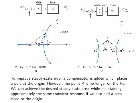
To improve steady-state error a compensator is added which placesa pole at the origin. However, the point A is no longer on the RL.We can achieve the desired steady-state error while maintainingapproximately the same transient response if we also add a zeroclose to the origin.

If the zero is close enough to the pole then θpc ≈ θzc which meansthey effectively cancel out, leaving A still on the RL. The requiredgain will be similar to the original system, since the ratio of themagnitudes of the added pole to the added zero is approx. 1.

e.g. The following system is operating with a damping ratio of0.174. Compensate the system to achieve estep(∞) = 0 whilemaintaining the system’s current transient response.

We first consider the RL of the uncompensated system...

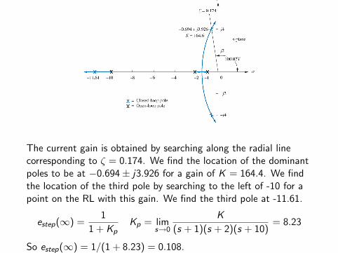
The current gain is obtained by searching along the radial linecorresponding to ζ = 0.174. We find the location of the dominantpoles to be at −0.694± j3.926 for a gain of K = 164.4. We findthe location of the third pole by searching to the left of -10 for apoint on the RL with this gain. We find the third pole at -11.61.

estep(∞) =1

1 + KpKp = lim

s→0

K

(s + 1)(s + 2)(s + 10)= 8.23

So estep(∞) = 1/(1 + 8.23) = 0.108.

We add an ideal integral compensator with a zero at -0.1.

This should have only a small effect on the system’s transientresponse characteristics. Consider the RL...

The gain K corresponding to ζ = 0.174 is now 158.2. This slightlyshifts the locations of the dominant poles and the third pole. Also,we now have a small section of the RL between the compensator’spole and zero. We search for it using the known value of K andfind it at -0.0902.

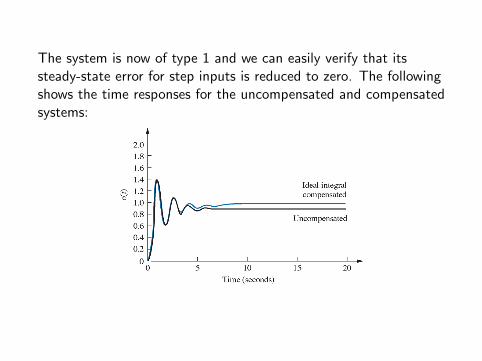
The system is now of type 1 and we can easily verify that itssteady-state error for step inputs is reduced to zero. The followingshows the time responses for the uncompensated and compensatedsystems:

Ideal integral compensation is also known as PI Control. Theproportional and integral components can be shown as separatetransfer functions in parallel.

The equivalent transfer function of the compensator is

Gc(s) = K1 +K2

s=

K1(s + K2K1

)

s

The location of the zero can be adjusted by adjusting K2/K1.

Lag Compensation

Ideal integral compensation requires an active circuit forimplementation. If this is not desirable then instead of placing apole directly at the origin we can try placing it very nearby. Ofcourse, we also place a zero nearby so as to minimize the impacton transient response. This is known as lag compensation.

The static error constant for the system is,

Kv =Kz1z2 · · ·p1p2 · · ·

With the lag compensator the static error constant becomes

Kvc =Kzcz1z2 · · ·pcp1p2 · · ·

=zc

pcKv

Thus, we get an increase in static error constant (decrease ineramp(∞)) when zc/pc is large. Are we free to choose how wemake this ratio large?

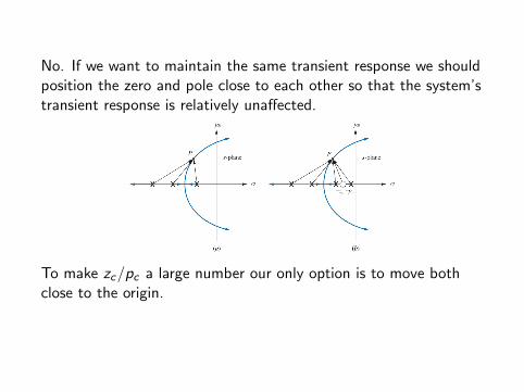
No. If we want to maintain the same transient response we shouldposition the zero and pole close to each other so that the system’stransient response is relatively unaffected.

To make zc/pc a large number our only option is to move bothclose to the origin.

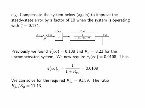
e.g. Compensate the system below (again) to improve thesteady-state error by a factor of 10 when the system is operatingwith ζ = 0.174.

Previously we found e(∞) = 0.108 and Kp = 8.23 for theuncompensated system. We now require ec(∞) = 0.0108. Thus,

e(∞)c =1

1 + Kpc

= 0.0108

We can solve for the required Kpc = 91.59. The ratioKpc/Kp = 11.13.

Since we previously found the following relationship,

Kvc =zc

pcKv

(The previously shown system was type 1 so we were discussing Kv

but in this example the system is type 0 so we are discussing Kp.)

zc/pc must equal the ratio Kpc/Kp. Arbitrarily choosing pc = 0.01we find,

zc = 11.13pc = 0.111

The root locus for the compensated system is as follows:

The following time response shows that the transient response isapproximately the same as the compensated system, while thesteady-state error has been significantly reduced.