uncertainties in prudence ... - the prudence project

Uncertainties in PRUDENCE simulations:

Global high resolution models

Michel Déqué

Contents1 Introduction..........................................................................................................................................32 Global domain......................................................................................................................................3

2.1 Global models...............................................................................................................................32.2 Systematic errors..........................................................................................................................42.3 Projection method.........................................................................................................................42.4 Projection of systematic errors.....................................................................................................5

2.4.a DJF 2m temperature..............................................................................................................52.4.b JJA 2m temperature..............................................................................................................62.4.c DJF 2m precipitation.............................................................................................................62.4.d JJA 2m precipitation.............................................................................................................6

2.5 Projection of climate impacts.......................................................................................................62.5.a DJF 2m temperature..............................................................................................................62.5.b JJA 2m temperature..............................................................................................................72.5.c DJF 2m precipitation.............................................................................................................72.5.d JJA 2m precipitation.............................................................................................................7

2.6 Mean and minimum response in PRUDENCE standard scenario................................................72.6.a DJF 2m temperature..............................................................................................................72.6.b JJA 2m temperature..............................................................................................................72.6.c DJF 2m precipitation.............................................................................................................82.6.d JJA 2m precipitation.............................................................................................................8

2.7 Four sources of uncertainty..........................................................................................................82.7.a DJF 2m temperature..............................................................................................................82.7.b JJA 2m temperature..............................................................................................................82.7.c DJF 2m precipitation.............................................................................................................82.7.d JJA 2m precipitation.............................................................................................................8

2.8 Synthesis.......................................................................................................................................93 Global models: European domain.......................................................................................................10

3.1 Projection of systematic errors....................................................................................................103.1.a DJF 2m temperature............................................................................................................103.1.b JJA 2m temperature............................................................................................................113.1.c DJF 2m precipitation...........................................................................................................113.1.d JJA 2m precipitation...........................................................................................................11

3.2 Projection of climate impacts......................................................................................................113.2.a DJF 2m temperature............................................................................................................113.2.b JJA 2m temperature............................................................................................................113.2.c DJF 2m precipitation...........................................................................................................123.2.d JJA 2m precipitation...........................................................................................................12

3.3 Mean and minimum response in PRUDENCE standard scenario..............................................123.3.a DJF 2m temperature............................................................................................................123.3.b JJA 2m temperature............................................................................................................123.3.c DJF 2m precipitation...........................................................................................................123.3.d JJA 2m precipitation...........................................................................................................12

3.4 Four sources of uncertainty........................................................................................................123.4.a DJF 2m temperature............................................................................................................123.4.b JJA 2m temperature............................................................................................................123.4.c DJF 2m precipitation...........................................................................................................133.4.d JJA 2m precipitation...........................................................................................................13

3.5 Synthesis.....................................................................................................................................13

1

4 Regional models: European domain...................................................................................................144.1 Projection of systematic errors....................................................................................................14

4.1.a DJF 2m temperature............................................................................................................154.1.b JJA 2m temperature............................................................................................................154.1.c DJF 2m precipitation...........................................................................................................154.1.d JJA 2m precipitation...........................................................................................................15

4.2 Projection of climate impacts.....................................................................................................154.2.a DJF 2m temperature............................................................................................................154.2.b JJA 2m temperature............................................................................................................154.2.c DJF 2m precipitation...........................................................................................................164.2.d JJA 2m precipitation...........................................................................................................16

4.3 Mean and minimum response in PRUDENCE standard scenario..............................................164.3.a DJF 2m temperature............................................................................................................164.3.b JJA 2m temperature............................................................................................................164.3.c DJF 2m precipitation...........................................................................................................164.3.d JJA 2m precipitation...........................................................................................................16

4.4 Four sources of uncertainty........................................................................................................174.4.a DJF 2m temperature............................................................................................................174.4.b JJA 2m temperature............................................................................................................174.4.c DJF 2m precipitation...........................................................................................................174.4.d JJA 2m precipitation...........................................................................................................17

4.5 Synthesis.....................................................................................................................................175 Conclusions........................................................................................................................................19

5.1 globe...........................................................................................................................................195.2 Europe.........................................................................................................................................19

6 References..........................................................................................................................................207 Figures: global domain.......................................................................................................................238 Figures: Europe (GCM).....................................................................................................................359 Figures: Europe (RCM)......................................................................................................................47

2

1 IntroductionGeneral Circulation Models (GCMs) coupled with dynamical ocean and sea-ice models offer aphysically-based approach to the large-scale response of the climate system to perturbations to theradiative cycle of the atmosphere by human activities (IPCC, 2001). At the European scale suchmodels are not accurate enough to take into account the complex orographic features which modulatestrongly the climate distribution. Regional Climate Models (RCMs), with meshes of a few tens ofkilometers are an adequate response to this challenge (Jones et al., 1997, Christensen et al., 2001). Infact, Europe is not the only place in the world where RCMs have proved successful (Giorgi et al.,1998, Laprise et al., 2003, Whetton et al., 2001, Fukutome et al., 1999). But a coordinated effort hasbeen undertaken in Europe since the mid-1990 (Machenhauer et al., 1998) to produce high quality,well documented, multi-model simulations. Regional model is used here as a generic term for a modeldesigned to simulate regional circulation features. RCMs can be limited area models (LAM, the mostusual approach) or global models with higher resolution in an area of interest (Déqué and Piedelievre,1995, Fox-Rabinovitz et al., 2001). Sensitivity studies with different resolutions (Lorant and Royer,2002 for variable resolution and Denis et al., 2003 for Limited Area Modeling) have shown that bothapproaches do not suffer from numerical artefacts due to discretization (at least no more than globaluniform grid models).

The PRUDENCE project is devoted to the study of anthropogenic climate changes over Europe. It hastwo main objectives: to estimate the uncertainties about the expected response, and to evaluatepossible impacts in various fields of human activities. The object of the present study is to focus onthe response of a few global General Circulation Models used in the project. The statistical method isthen applied to the RCMs of the PRUDENCE project. As the method is rather comprehensive from astatistical point of view, we will restrict to 30-year seasonal means. Moreover, amongst the manyfields archived in the PRUDENCE database, we select 2m temperature and precipitation. These fieldsoffer the triple advantage to be directly connected to human perception of the climate, to becomparable with reliable observation, and to exhibit regional-scale features that are not accessible tocoarse resolution GCMs. In order to further reduce the size of this report, we concentrate on the twoextreme seasons boreal winter (DJF) and summer (JJA).

The report is organized in 3 parts. In the first part, we analyze the four global high resolution modelsavailable over the globe. In the second one, the same models receive the same statistical treatmentafter restriction to the European domain. In order to compare the results we obtain with those ofRCMs, a third part extends the regional statistical analysis to the ten RCMs of the PRUDENCEproject.

2 Global domain

2.1 Global models

Although PRUDENCE is focused on climate modeling over Europe, global models have been used inthis project. The aim of this report is to investigate the systematic errors and the climate sensitivity ofthe global models. Global models are necessary in regional modeling:• to provide in any case a sea surface temperature (SST) through a coupled ocean-atmosphere model• to provide, in the case of LAM, driving atmospheric boundary valuesThe RCM used by Centre National de Recherches Météorologiques (CNRM) is ARPEGE-Climate.3(Gibelin and Déqué, 2003), a global model with spectral TL106 truncation (120 latitudes and 240longitudes grid). Its resolution of 0.50° over southern Europe due to grid-stretching makes itcomparable with other LAMs of the project. The global model used in PRUDENCE to drive theLAMs in the standard scenario is HadAM3, developed by Hadley Centre. Its horizontal resolution is1.24° over Europe, as well as any part of the mid-latitudes (145 latitudes and 192 longitudes grid). Athird global model is the NCAR Community Climate Model, developed in the US and used at ICTP

3

(181 latitudes by 288 longitude grid). Its horizontal resolution is 1° in the mid-latitudes. A fourthglobal model is used in the project to provide boundary conditions. ECHAM5 is developed by MPI. Ituses a T106 spectral truncation (160 latitudes and 320 longitudes grid). Its resolution is 1.12° overEurope, as well as in any part of the globe.These four models have been used in a control simulation of 30 years, driven by monthly observedSSTs of the 1961-1980 period. In the case of CNRM and Hadley Centre, an ensemble of 3simulations is available. In the case of ICTP model, we have 2 simulations.

2.2 Systematic errors

The first source of credibility for a GCM is a fair adequacy between the mean simulated climate andthe observed one. We restrict here to four fields: 2m temperature and precipitation in DJF and JJA. Itis relatively easy to choose a set of empirical parameters which provide a good fit on a particular areaof the globe. For example the convection scheme may be tuned to provide the right rainfall amountover India during the monsoon season. But if this choice is not physically consistent, large errors willappear in other areas or other seasons. For this reason, a small error all over the globe is a goodcriterion of the degree of realism of an atmosphere model. LAMs do not allow such a severeverification. A simple verification tool is the root mean square (RMS) difference over the globe withan observed climatology. The climatology we use here is Legates and Willmott (1990) fortemperature and Xie and Arkin (1996) for precipitation. All fields are interpolated onto a commongrid with 128 longitudes and 64 latitudes.

2.3 Projection method

We could give here the 16 systematic errors (4 models, 2 fields, 2 seasons), but this is important toknow how far the models are from each other. Indeed, if the models have similar systematic errors,our confidence in the agreement between the simulated climate changes will we lower. Similarmodels producing similar systematic errors are expected to produce similar responses to greenhousegas increase. In our case, we have four models. If we had only three models, the three points in the128x64-dimensional space would be in a plan. They could be thus plotted in a 2d figure. We couldproject onto this plan the climatology, in order to see the respective location of the three models withrespect to the climatology, having in mind that the distance between the climatology point and amodel point is not the RMS error, but a smaller value:

d=RMSE 2−a2 (1)where a is the distance between the climatology and the plan of the three models. However the largerthe RMS error, the larger the distance.But we have more than three models, and the points representing the different models do not fit on aplan, unless very particular configurations. There exists a statistical technique, namedMultidimensional Scaling (MDS: Rencher, 2002), which uses the true distances d ij of n points tocalculate virtual positions in a subspace ℝk so that the euclidean distances in ℝk are as close aspossible to the original distances. Practically, k is taken as 2, but sometimes a 3-d space can beconsidered and the three 2-d projections can be plotted. The d ij are not necessarily euclideandistances (like the RMS difference), but can be based on mean absolute error or pattern correlation.However, in the case of euclidean distances the MDS comes to an EOF analysis, which offers twoadvantages:• the point representing a new model climatology (or any kind of map) can be calculated by linear

combinations• the two axes of the plan can be plotted as geographic mapsLet X(i,x) be the value of field X (e.g. 2 m temperature in DJF) for model i (i=1,...,n) at location x (xrepresenting here the latitude longitude pair). Let s(x) be the surface of the mesh corresponding to x.The mean field (centroid) is:

4

X x=1 n ∑i=1

n

X i , x (2)

and the matrix to be diagonalized is:

V ij=∑x

s xX i , x−X xX j , x−X x (3)

Let v k i be the k-th eigenvector (with norm 1) associated to the eigenvalue k (the eigenvaluesbeing sorted in decreasing order. Then the k-th axis for the projection is:

Ak x=∑i=1

n

v k iX i , x−X x (4)

The point representing model i is ( 1 v1i , 2 v2i ) and the coordinates of the pointrepresenting a new field Y(x) (k=1 or 2):

yk=1

k

∑x

s x Ak xY x−X x (5)

In the case of a non-euclidian distance, Eqs. (2) to (5) are no more valid since we use the array d ij

of the distances between the models, which is no more a quadratic combination of the array X(i,x).Eq. (3) is replaced by

V ij=12{1n∑h

d hj2 1

n∑k

d ik2 −d ij

2− 1

n2∑hk

d hk2 } (6)

and the eigenvectors of V ij scaled by the square root of the (sorted) eigenvalues provide thecoordinates of the representative points. In this note, we use only euclidean distances.

2.4 Projection of systematic errors

In fact, we have more than 4 systematic error maps to project, because of the ensemble experiments.We have 9 different maps (3+3+2+1). But ICTP and MPI RMSE maps have been replicated so thateach model has the same weight (i.e. 3 members). We thus process 12 maps of size 128x64.

2.4.a DJF 2m temperature

Figure 1a shows the distribution of the biases of the 4 models for 2m temperature in DJF. Themembers of a same ensemble (CNRM, Hadley Centre or ICTP) are very close together. This showsthat a 30-year length is sufficient to capture the model climatology with accuracy. The MPI model(letter D) is the closest to observed climatology. MPI and CNRM models are spread along the x-direction, Hadley Centre with a negative x-component, CNRM with a positive one. The ICTP modelis shifted in the y-direction. Figure 2a shows the mean error. It corresponds to the gravity center ofABCD points in Figure 1a. The mean model is too cold over Africa, Greenland, Tibet, and too warmin Siberia and over the sea-ice. Figure 2b shows the x-axis, which makes the difference betweenCNRM and Hadley Centre models. The axis is counted positively from left to right, so that CNRMmodel is colder than Hadley Centre model over Africa. The length of the light gray arrow on the leftof the panel corresponds to 1K (in any direction). The map and the projection are scaled both by1 so that they are expressed in K. If one wants to combine the x-value with the map of

Figure 2a, it has to be normalized by 2.1K. Similarly, the y-value has to be divided by 2.5K in areconstruction of the systematic error of model i by:

E i , x=E xA1 xv1i

1

A2 xv2i

2

(7)

Figure 2a corresponds to the mean E x . Figure 2b corresponds to the x-axis A1 x . Figure 2ccorresponds to the y-axis A2 x . It is oriented upwards, so that Hadley Centre model is warmerthan ICTP model over East America and East Asia. The projection along the two axes corresponds to78% of the variance. It would be 100% with 3 points to be projected, but we have here nine different

5

points. In the whole document, the scale is larger in the y-direction ( 12 ) to fit with the portraitformat of the plots.

2.4.b JJA 2m temperature

In JJA, the positions change (Figure 1b). Now CNRM and ICTP models are closest to observation.The mean error (Figure 2d), the x-axis (Figure 2e) and the y-axis (Figure 2f) are completely differentfrom the DJF case. The standard deviations along the two axes are 2.4K and 3.3K. These two axescorrespond to 82% of the variance.

2.4.c DJF 2m precipitation

DJF precipitation is projected in Figure 1c. The four models are spread about the observation, HadleyCentre model being the closest. The length of the arrow corresponds to 1mm/day. The mean error(Figure 3a) shows an excessive precipitation, except along the equator. The x- and y- axes correspondto complex structures. The respective scalings are 1.9 and 2.0 mm/day. These two axes explain 75%of the variance.

2.4.d JJA 2m precipitation

In JJA, the position of the four models about observation is shown in Figure 1d. The mean error andthe axes (Figures 3d, 3e and 3f) are rather different. The scale of the x- and y-axes is 2.1 and 2.5mm/day. The two axes explain 78% of the variance.

2.5 Projection of climate impacts

The method used in section 2.4 can be applied to summarize in a few plots the behavior of the fourGCMs. In this section we consider the impact maps, i.e. the difference between the perturbed climateand the control climate. For the CNRM model, we have three simulations with A2 scenario andHadley Centre SST, one simulation with A2 scenario and CNRM SST (coming from a low resolutioncoupled run of the same model), one simulation with B2 scenario and Hadley Centre SST, and threesimulations with B2 scenario and CNRM SST. For the Hadley Centre model, we have threesimulations with A2 scenario and Hadley Centre SST, one simulation with B2 scenario and HadleyCentre SST. As far as ICTP is concerned, we have two simulations with A2 scenario and HadleyCentre SST. For the MPI, we have just one simulation with A2 scenario and Hadley Centre SST.ICTP (resp. MPI) first maps have been duplicated (resp. triplicated), so that the four models have thesame weight, as far as the standard PRUDENCE experiment (A2, Hadley Centre SST) is concerned.We have thus 21 maps to project onto a 2-d space, out of which 12 correspond to the standard A2scenario.


Figure 4a shows the relative position of the various impacts. One first remark is that the members of asame ensemble are close to each other. Here again, 30 years are sufficient to estimate an accurateseasonal mean. The A2 scenario points (red letters) are located in the same region and spread alongthe x-axis. The present climate (letter P) is on the opposite side of this axis. It corresponds to theprojection of a map with zero values everywhere. The B2 scenario with Hadley Centre SST (blueupper case letters) is on an intermediate position along this axis, which shows the scalability of thepattern. Using CNRM SST (lower case letters) moves the points along the y-axis, resulting in a largerimpact, when the distance to the present climate is considered. The mean model impact (Figure 5a)shows an overall warming, with a maximum over polar winter latitudes and a minimum over theoceans. The x-axis (Figure 5b, scale 1.6K) is negative over all continents. This is quite normal, as theobservation is on the right-hand side of this axis. As the models use the same SST anomaly for agiven scenario, it is expected that this axis has no signal on the ocean. On the contrary, the y-axis(Figure 5c, scale 3.3K) has also a signal over the oceans, but mainly over the winter sea-ice. Indeed

6

the CNRM coupled simulations have produced a very strong decrease of the sea-ice in the scenarios,whereas Hadley Centre scenarios are very conservative. Surprisingly, the B2 scenario has an evenstronger impact: this can be explained by a change in the CNRM sea-ice model in the A2 coupledsimulation (which was performed later), resulting in a more conservative sea-ice. The two axesexplain 79% of the variance.


The mean response for all model and scenarios is shown in Figure 5d. The warming is maximum overthe Antarctic and the northern midlatitude continents. Figure 4b shows the relative position of thevarious impacts. Contrary to DJF case (Figure 4a), the present climate is on the left-hand side. In factthe sign of the eigenvectors being arbitrary, the algorithm provides a random value for the sign of themaps. As a consequence, the x-axis (Figure 5e) is mostly positive. If we exclude the Antarctic, this x-axis corresponds to the differences in warming intensity over Europe. Its scale is 1.7K. The y-axis(Figure 5f, scale 3.7K) is rather similar to the corresponding DJF pattern. The two axes explain 81%of the variance.


Figure 4c shows the relative position of the various impacts. The scenarios using CNRM SST (lowercase characters) are close to present climate, indicating a weak response (at least after projection)whatever the scenario A2 or B2. For the upper case characters (Hadley Centre SST forcing), B2scenarios (blue characters) are aligned with the A2 ones (red characters), indicating a scalability of theresponse. The two axes (Figures 6b and 6c) show complex pattern. Their scale is 1.3 mm/day (x-axis)and 1.6 mm/day (y-axis). They explain 60% of the variance.


Figure 4d shows the relative position of the various impacts. We have a very similar situation as inDJF. A noticeable difference is the mean impact pattern (Figure 6d) over Europe. The two axes havea scale of 1.4 and 1.7 mm/day and explain 59% of the variance.

2.6 Mean and minimum response in PRUDENCE standard scenario

The PRUDENCE standard scenario is the IPCC-A2 radiative forcing and the Hadley Centre SST. Wehave 12 simulations of this scenario (in the case of MPI and ICTP models, some simulations arerepeated) and 12 control simulations. The difference provides the mean climate response. But we canconsider that the mean anomaly is an average of four independent anomalies. An unbiased estimate ofthe inter model standard deviation i has been calculated at each grid point. The standard deviationof the ensemble mean is thus m=i /4 . A minimum expected response can be evaluated (at the97.5% threshold) by the following way: if the mean response m is positive, we take m−2m ,otherwise we take m2m . This is coarse statistics (it will be more accurate with ten RCMs insection 4), but is a simple way to evaluate the regions where the models are in agreement.


Figure 7a shows the mean response of all the A2 scenarios with Hadley Centre SST. It is differentfrom Figure 5a which includes the B2 and the CNRM SST impacts. But the differences are marginal.Figure 7c shows how this impact is reduced when taking into account the uncertainty between the 4models. The amplitude reduction is modest.


Figures 7b and 7d show the same thing for JJA. The same conclusions as in the DJF case can bedrawn.

7


Figure 8a shows the mean response of all the A2 scenarios with Hadley Centre SST. Figure 8c showshow this impact is reduced when taking into account the uncertainty between the 4 models. Theamplitude reduction is larger than in the temperature case.


Figures 8b and 8d show the same thing for JJA. The same conclusions as in the DJF case can bedrawn.

2.7 Four sources of uncertainty

We can go one step further than in section 2.6 in the uncertainty analysis by using the ensembles andthe other scenarios. There are 15 different anomaly maps available. Let us consider the 105 possibledifferences between pairs of map:• if the model, the radiative forcing (A2 versus B2), and the SST are the same, the difference is said

to be due to sampling• if the model and the radiative forcing are the same, and the SST is different, the difference is said to

be due to SST• if the model and the SST are the same, and the radiative forcing is different, the difference is said to

be due to radiative forcing• if the radiative forcing and the SST are the same, and if the model is different, the difference is said

to be due to the modelFor each of the four types of differences, a quadratic average is calculated at each grid point. Here thesampling is poor, but in section 4.4 this approach is more accurate. Dividing this mean difference by2 provides the standard deviation due to each source. One could consider differences involving at

a time a different model, a different scenario and a different SST to express a “total” uncertainty, butthe 4 sources are not additive and one can even find cases for which, due to poor sampling and to thefact that the different sub-populations have different distributions, one of the 4 sources has a largerstandard deviation than the “total” uncertainty.


Figures 9a to 9d show the impact of the 4 sources of uncertainty. The sampling is negligible andlocated in the northern midlatitude continents. The radiative uncertainty (A2 versus B2) is spread overland as well as over sea, with a maximum over the Arctic. The SST uncertainty is essentially locatedin the sea-ice regions. The model uncertainty is located over continent. See section 2.8 for a numericalcomparison of the 4 sources.


The geographical distribution is shown in Figures 9e to 9h. The main features as in DJF are observed,except some hemisphere changes due to winter/sumer contrasts.


Figures 10a to 10d show the uncertainty in the precipitation impact. The sampling error is no morenegligible. The four patterns are similar and correspond to the rainy areas (storm tracks and ITCZ).


The geographical distribution is shown in Figures 10e to 10h. The main features as in DJF areobserved, except some enhancements in the tropics.

8

2.8 Synthesis

The projection method used in sections 2.4 and 2.5 is based on a reduction to a plan. It introduces thusan approximation. Moreover, the observation or the present climate are not used in the mattrix to bediagonalized, for the sake of symmetry. Thus, the distances to point O (Figure 1) or to point P(Figure 4) are not accurate on the diagrams. Tables 1 to 4 show the exact mean quadratic distances forthe 4 models: distance to observed climatology (Clim.), A2 scenario with Hadley Centre SST (A2),A2 with CNRM SST (A2*), B2 scenario with Hadley Centre SST (B2), and B2 with CNRM SST(B2*). It can be checked that the close vicinity of the scenarios using CNRM SST to the unperturbedclimate (Figures 4c and 4d) for precipitation is an effect of the projection.

A B C D

Clim. 3.4 3.2 3.3 2.9

A2 3.7 3.9 3.6 3.7

A2* 3.9

B2 2.8 2.8

B2* 4.1

Table 1: Exact distances over the globe between the simulated present climate and observed climatology(Clim.) and between the 4 scenarios (when available) and the simulated present climate (A2, A2*, B2,B2*): A=CNRM, B=Hadley Centre, C=ICTP and D=MPI. Temperature in DJF (K).

A B C D

Clim. 3.4 3.9 3.2 3.6

A2 3.4 3.6 3.7 3.2

A2* 3.9

B2 2.6 2.6

B2* 3.4

Table 2: As Table 1 for JJA temperature (K).

A B C D

Clim. 1.7 1.2 1.7 1.5

A2 0.9 0.9 1.1 1.1

A2* 0.5

B2 0.7 0.7

B2* 0.4

Table 3: As Table 1 for DJF precipitation (mm/day).

A B C D

Clim. 1.6 1.4 1.7 1.9

A2 1.0 1.0 1.3 1.2

A2* 0.6

B2 0.8 0.8

B2* 0.4

Table 4: As Table 1 for JJA precipitation (mm/day).

9

The global warming in the A2 scenario is 3.3K in both DJF and JJA, when the average of the fourmodels is considered. The minimum expected impact (average of Figures 7c and 7d) is 2.8K (DJF)and 2.5K (JJA). This shows a larger uncertainty due to models in JJA. As far as precipitation isconcerned, global averaging cancels out positive and negative impacts. The net effect is an increase inglobal precipitation (0.2 mm/day), which is statistically significant, since the minimum impact ispositive as well (0.1 mm/day).

Table 5 summarizes the quadratic global averages obtained in the previous results. The first columnindicates the RMSE of the mean model, which is different from the mean RMSE of the four models.The next column indicates the response of the mean model. These first two columns correspond to thefirst two rows of Tables 1 to 4 for the mean model. The next four columns correspond to the quadraticglobal averages of the 4 standard deviations (sampling, radiative forcing, sea surface temperature, andmodel). The last column corresponds to the standard deviation used to evaluate the minimumexpected response (Figures 7c, 7d, 8c and 8d). It makes little sense to merge the four standarddeviations, as only one model is using two types of SST, two models use the two types of radiativeforcing, and three models have more than one sample.

bias impact SD1 SD2 SD3 SD4

DJF temperature (K) 3.0 3.9 0.3 1.1 1.9 0.8

JJA temperature (K) 3.3 3.7 0.3 0.8 2.0 1.3

DJF precipitation (mm/day) 1.2 0.7 0.3 0.3 0.5 0.6

JJA precipitation (mm/day) 1.2 0.8 0.2 0.3 0.5 0.6

Table 5: Quadratic average over the globe of bias and impact of the A2/Hadley Centre SST scenario forthe mean model. Standard deviations due to sampling (SD1), radiative forcing (SD2), SST forcing (SD3)and model (SD4).

3 Global models: European domainWe consider here the same experiments as in section 2, but we apply the methods to data interpolatedonto a 0.5°x0.5° grid covering Europe from 75°N, 15°W to 35°N, 35°E. The observed climatology isthe CRU one (Hulme et al., 1995) for 2m temperature as well as precipitation. It does not provide dataover the oceans, thus the systematic error analysis is done for the land part of this domain.



Figure 11a shows the distribution of the biases of the four models for 2m temperature in winter. Themembers of a same ensemble (CNRM, Hadley Centre or ICTP) are very close together. This showsthat a 30-year length is sufficient to capture the model climatology with accuracy, even on a regionaldomain. The Hadley Centre and MPI models (letters B and D) are closest to observed climatology.ICTP and CNRM models are spread along the y-direction, ICTP with a negative y-component,CNRM with a positive one. The other two models are shifted rightwards. Figure 12a shows the meanerror. It corresponds to the barycenter of ABCD in Figure 11a. The mean model is close toclimatology. Figure 12b shows the x-axis, which makes the difference between CNRM and MPImodels. The axis is counted positively from left to right, so that MPI model is warmer than CNRMmodel over Sweden. The length of the light gray arrow on the left of the panel corresponds to 1K (inany direction). The map and the projection are scaled both by 1 so that they are expressed in K. Ifone wants to combine the x-value with the map of Figure 12a, it has to be normalized by 2.0K.Similarly, the y-value has to be divided by 2.9K in a reconstruction of the systematic error of a model

10

by Eq. (7). Figure 12c corresponds to the y-axis A2 x . It is oriented upwards, so that CNRMmodel is warmer than ICTP model in the North and colder in the South. The projection along the twoaxes corresponds to 76% of the variance, which is similar to what we got for the globe.Note that the absence of colour over the seas is simply due to the fact that the CRU climatology isavailable only over land.


In summer, the positions change (Figure 11b). Now CNRM model is the closest to observation. Themean error (Figure 12d) shows a warm bias in the South and a cold bias in the North. The x-axis(Figure 12e) and the y-axis (Figure 12f) are completely different from the winter case. The standarddeviations along the two axes are 1.8K and 3.2K. These two axes correspond to 87% of the variance.


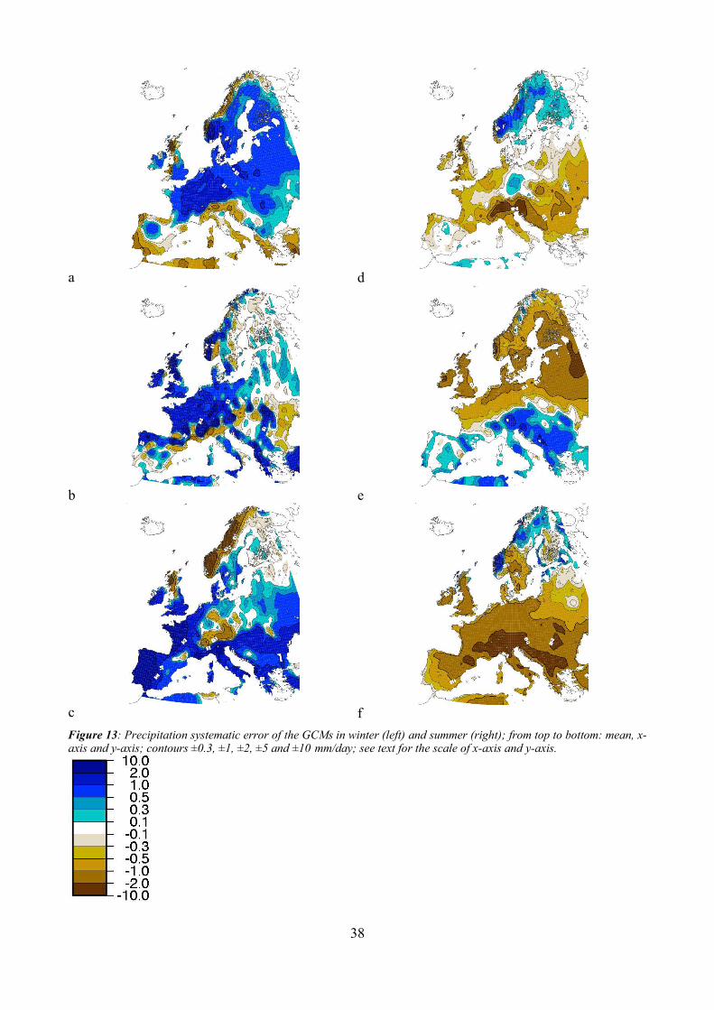
Precipitation biases are projected in Figure 11c for the winter case. The MPI model is the closest toobservation. The length of the arrow corresponds to 0.5 mm/day. The mean error (Figure 13a) showsan excessive precipitation, except around the Mediterranean sea and along the Norwegian coast. Therespective scales of the x- and y- axes are 1.0 and 1.3 mm/day. These two axes explain 89% of thevariance, which is much more than for the global maps.


In summer, the position of the four models about observation,(Figure 11d) and the mean error(Figure 13d) are rather different. The CNRM model is the closest to observation. The mean bias is adrying everywhere, except over Scandinavia. The two axes of the projection (Figures 13e and 13f)have some similarity (having in mind that the sign is arbitrary) with the winter ones. The scale of thex- and y-axes is 0.9 and 1.3 mm/day. The two axes explain again 89% of the variance.



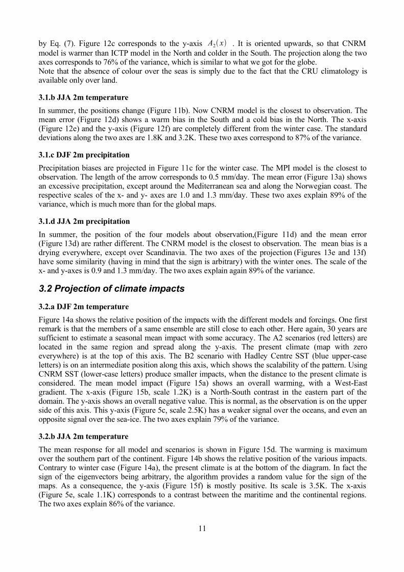
Figure 14a shows the relative position of the impacts with the different models and forcings. One firstremark is that the members of a same ensemble are still close to each other. Here again, 30 years aresufficient to estimate a seasonal mean impact with some accuracy. The A2 scenarios (red letters) arelocated in the same region and spread along the y-axis. The present climate (map with zeroeverywhere) is at the top of this axis. The B2 scenario with Hadley Centre SST (blue upper-caseletters) is on an intermediate position along this axis, which shows the scalability of the pattern. UsingCNRM SST (lower-case letters) produce smaller impacts, when the distance to the present climate isconsidered. The mean model impact (Figure 15a) shows an overall warming, with a West-Eastgradient. The x-axis (Figure 15b, scale 1.2K) is a North-South contrast in the eastern part of thedomain. The y-axis shows an overall negative value. This is normal, as the observation is on the upperside of this axis. This y-axis (Figure 5c, scale 2.5K) has a weaker signal over the oceans, and even anopposite signal over the sea-ice. The two axes explain 79% of the variance.


The mean response for all model and scenarios is shown in Figure 15d. The warming is maximumover the southern part of the continent. Figure 14b shows the relative position of the various impacts.Contrary to winter case (Figure 14a), the present climate is at the bottom of the diagram. In fact thesign of the eigenvectors being arbitrary, the algorithm provides a random value for the sign of themaps. As a consequence, the y-axis (Figure 15f) is mostly positive. Its scale is 3.5K. The x-axis(Figure 5e, scale 1.1K) corresponds to a contrast between the maritime and the continental regions.The two axes explain 86% of the variance.

11


Figure 14c shows the relative position of the various impacts. There is a large spread, but all scenariosare on the right-hand side of the present climate. The scenarios using CNRM SST (lower-casecharacters) are at the bottom of the diagram. For the upper-case characters (Hadley Centre SSTforcing), B2 scenarios (blue characters) are aligned with the A2 ones (red characters), indicating ascalability of the response. The two axes (Figures 16b and 16c) show a NW-SE and a SW-NE patternrespectively. Their scale is 0.5 mm/day (x-axis) and 0.7 mm/day (y-axis). They explain 65% of thevariance.


Figure 14d shows the relative position of the various impacts. We have a distribution of points similarto the winter one, but rotated (the present climate is at the bottom). A noticeable difference is themean impact pattern (Figure 16d) which corresponds to a drying. The y-axis (Figure 16f) is similar tothe mean impact, so that it controls the intensity of the response: Hadley Centre (B) has the strongestdrying. The two axes have a scale of 0.5 and 0.7 mm/day and explain 70% of the variance.



Figure 17a shows the mean response of all the A2 scenarios with Hadley Centre SST. It is differentfrom Figure 15a which includes the B2 and the CNRM SST impacts. But the differences are small:with A2 only, a warmer impact is obtained. Figure 17c shows how this impact is reduced when takinginto account the uncertainty between the 4 models. The amplitude reduction is not dramatic.


Figures 17b and 17d show the corresponding maps for summer. The warming over southern Europe isat least 4K. The warming over the Baltic sea is a typical feature of the Hadley Centre SST.


Figure 18a shows the mean response of all the A2 scenarios with Hadley Centre SST. Figure 18cshows how this impact is reduced when taking into account the uncertainty between the 4 models. Theamplitude reduction is larger than in the temperature case.


Figures 18c and 18d show that the precipitation decrease is not significant. The only robust feature insummer is the precipitation increase over the Baltic sea, due to warm SST.



Figures 19a to 19d show the impact of the 4 sources of uncertainty. The sampling is negligible andlocated in the eastern part. The radiative uncertainty (A2 versus B2) is spread over land. The SSTuncertainty is essentially located in the sea-ice regions. The model uncertainty is located overcontinent and is dominant in winter. See section 3.5 for a numerical comparison of the 4 sources.


The geographical distribution is shown in Figures 19e to 19h. The main winter features are recovered,except some impact of the SST forcing.

12


Figures 20a to 20d show the uncertainty in the precipitation impact. The sampling error is no morenegligible. The four patterns are similar and correspond to the rainy areas (mountains and coasts).


The geographical distribution is shown in Figures 20e to 20h. The main winter features are obtained,except some enhancements in the Baltic sea.

3.5 Synthesis

Tables 6 to 9 give the exact distances, the approximation of which can be seen in Figures 11 and 14.This concerns only the distance present-observation (first row) and the distances scenario-present(next four rows). The distances between individual models are not reported.

A B C D

Clim. 1.8 1.8 1.9 1.7

A2 3.4 3.9 3.5 3.6

A2* 3.2

B2 2.8 2.9

B2* 3.2

Table 6: Exact distances over Europe between the simulated present climate and observed climatology(Clim.) and between the 4 scenarios (when available) and the simulated present climate (A2, A2*, B2,B2*): A=CNRM, B=Hadley Centre, C=ICTP, D=MPI. Temperature in DJF (K).

A B C D

Clim. 1.3 1.8 2.4 2.5

A2 3.7 5.0 4.0 3.8

A2* 3.4

B2 2.8 3.6

B2* 2.7


A B C D

Clim. 1.0 0.9 1.0 0.9

A2 0.6 0.5 0.6 0.5

A2* 0.4

B2 0.5 0.3

B2* 0.4


13

A B C D

Clim. 0.6 0.8 0.8 1.1

A2 0.4 0.5 0.5 0.3

A2* 0.3

B2 0.3 0.3

B2* 0.2


The mean warming over Europe is 3.4K in winter and 3.8K in summer. The corresponding minimumvalues are 2.8K and 3.0K. The warming has a W-E gradient in winter, due to the snow feedback andthe ocean tempering role. It has a N-S gradient in summer, due to the drying out of southern regions.The precipitation increase in winter is 0.2 mm/day, its minimum expected value (average of meanplus or minus two standard deviation) is 0.1 mm/day. In summer, the mean impact on precipitation isa reduction by 0.1 mm/day. But this impact is not significant, as the minimum expected impact is veryclose to zero.

Table 10 summarizes the area quadratic averages obtained in the various approaches. The first columnindicates the RMS error of the mean model. The next column indicates the quadratic response of themean model. The next 4 columns correspond to the quadratic regional averages of the 4 standarddeviations (sampling, radiative forcing, sea surface temperature, and model). Note that the average inthe first column does not take into account the sea region, where the CRU climatology is notavailable.






Table 10: Quadratic average over Europe of bias and impact of the A2/Hadley Centre SST scenario forthe mean GCM. Standard deviations due to sampling (SD1), radiative forcing (SD2), SST forcing (SD3)and model (SD4).

4 Regional models: European domainWe use here the ten RCMs available in the PRUDENCE seasonal database. The models are those ofCNRM (the same simulations as in section 2 and 3), DMI, ETHZ, GKSS, Hadley Centre, ICTP,KNMI, MPI, SMHI and UCM. The resolution is, as in section 3, 0.5°x0.5°. However the domain isslightly smaller, as we must consider the intersection of all LAMs: the latitudes beyond 65°N havebeen removed. As in section 3, ocean points are not considered in the analysis of systematic errors.


Out of the ten RCMs, three models (CNRM, DMI and Hadley Centre) have produced three 30-yearreference simulations. For the other seven, we have triplicated the single reference simulation in orderto give the same weight to each model. Contrary to the case of four models, the projection along twoaxes leads to neglecting more than 40% of variance, so that the distances we analyze on the diagramsare not as accurate as in section 3 where about 20% of the variance was neglected in the projection.

14


Winter temperature systematic errors project in a rectangle of 1K by 2K size. The observed climate isat the top left corner. The mean bias (Figure 22a) exhibit a slightly warm error in the northern half ofEurope. The x-axis (Figure 22b) is a contrast between Mediterranean and Scandinavian regions. Itsscaling factor is 1.9K. The DMI model is on the leftmost part, ICTP and KNMI models on therightmost one. The y-axis (Figure 22c) corresponds to overall cooling from bottom (MPI model) totop (CNRM model). The scaling factor is 2.9K. The two axes explain only 51% of the variance.


In summer (Figures 21b, 22d, 22e and 22f) we observe similar patterns except that the warm bias overScandinavia is displaced in South East Europe. The x-axis (scale 2K) and y-axis (scale 3.3K) explain61% of the variance. The ten models occupy a different position than in winter in the 2-d projection.


Winter precipitation biases (Figure 21c) are spread about the observation. The mean error (Figure 23a)is a wet bias over the central and northern part and a dry bias along the Mediterranean coast. The x-axis (Figure 23b, scaling 1.5 mm/day) corresponds to a dry anomaly over the mountains. The y-axis(Figure 23c, scaling 2.1 mm/day) corresponds to a dry anomaly over the mountains, associated to wetanomalies in the rest of the continent. The two axes explain 56% of the variance.


Summer precipitation biases ( Figure 21d) cluster about the observed climatology, UCM model beingisolated. The mean error (Figure 23d) is a dry bias over South East Europe. The x-axis (Figure 23e,scaling 1.3 mm/day) corresponds to a dry anomaly over the south, except the Alps. The y-axis(Figure 23c, scaling 2.0 mm/day) corresponds to a wet anomaly over central and northern Europe: itshows that UCM model is drier than the other models and observation. The two axes explain 63% ofthe variance.


There are 26 anomaly maps avalaible from the PRUDENCE database, from which 13 follow thestandard PRUDENCE scenario. If we triplicate the A2 scenarios with Hadley Centre SST for theseven models which have run a single experiment, we can consider in addition to the standardPRUDENCE experiments:• the five CNRM simulations considered in the previous sections (one A2 and four B2)• one A2 simulation with MPI SST by DMI RCM• one A2 simulation with MPI SST by SMHI RCM• one B2 simulation with Hadley Centre SST by Hadley Centre RCM• one B2 simulation with Hadley Centre SST by SMHI RCM• one B2 simulation with MPI SST by SMHI RCM


The impact in winter temperature form a cluster along the y-axis (Figure 24a). The B2 scenarios arealong the same axis, closer to present climate than the A2 ones. The mean impact map (Figure 25a)shows a West-East gradient in the warming. The x-axis (Figure 25b, scale 1.2K) corresponds to acontrast between the North-East and the South-East. The y-axis (Figure 25c, scale 3.2K) correspondsto a continental warming. The two axes explain 84% of the variance.


The impact in summer temperature also form a cluster along the y-axis (Figure 24b). The mean

15

impact map (Figure 25d) shows a North-South gradient in the warming. The x-axis (Figure 25e, scale1.7K) corresponds to a contrast between the Baltic and Black Sea on one side and the Atlantic Oceanon the other side. The y-axis (Figure 25f, scale 4.5K) corresponds to a continental warming. The twoaxes explain 79% of the variance.


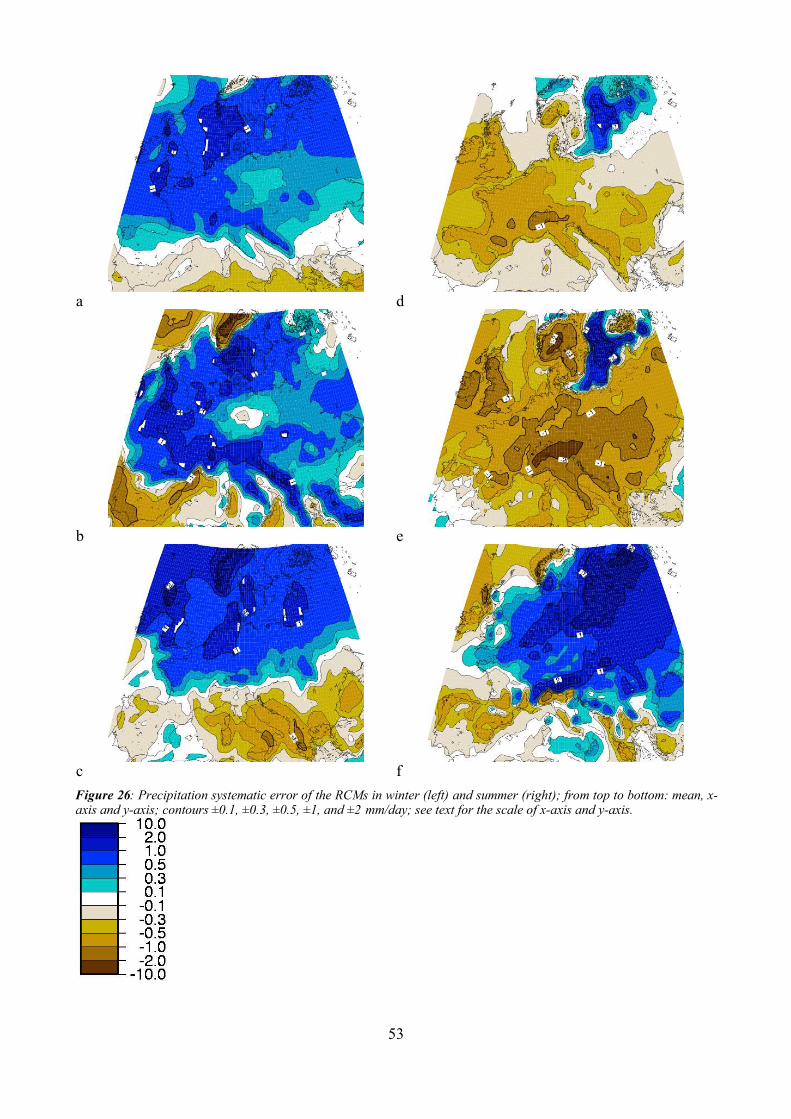
The winter precipitation impacts (Figure 24c) have a large spread, but are located in the samequadrant with respect to present climate. The discrimination between A2 and B2 scenarios is clear,except CNRM A2 scenario with CNRM forcing which lies in the region of the B2s, and the SMHI B2with MPI forcing which lies in an extreme position (the SMHI A2 with MPI forcing is even moreextreme). The mean impact map (Figure 26a) shows an overall precipitation increase, except in theMediterranean sea. The x-axis (Figure 26b, scale 0.8 mm/day) corresponds to a similar pattern. The y-axis (Figure 26c, scale 0.9 mm/day) corresponds to a North-South contrast. The two axes explain 51%of the variance.


The summer precipitation impact distribution (Figure 24d) offers the same kind of scatter than inwinter, except that the SMHI scenarios with MPI forcing are no more isolated. The mean impact(Figure 26d) is a reduction of precipitation everywhere except over the Baltic sea. The x-axis(Figure 26e, scale 0.9 mm/day) serves to modulate this mean impact. The y-axis (Figure 26f, scale 1.2mm/day) corresponds to contrast between the continental and oceanic areas. The two axes explain59% of the variance.



The winter mean temperature shown in Figure 27a corresponds only to A2 scenarios with HadleyCentre forcing (contrary to Figure 25a which includes all scenarios). It has however many similarities,with the West-East gradient due to the snow-albedo effect and to the tempering role of the ocean.When two standard deviations are subtracted (Figure 27c), the attenuation is marginal, as we havehere ten models (contrary to Figure 17a versus Figure 17c).


A similar conclusion may be drawn for summer temperature (Figures 27b and 27d), except that thegradient is North-South, due to the soil drying-out mechanism in the southern part of Europe.


The mean impact of the A2 scenario with Hadley Centre forcing (Figure 28a) is a precipitationincrease in the major part of the domain and a decrease over the Mediterranean Sea. The minimumimpact (Figure 28c) is hardly 0.1 mm/day over this region, but we can at least exclude an increase inwinter Mediterranean precipitation in the A2 scenario.


In summer (Figures 28b and 28d), precipitation is significantly reduced over the western and southernpart of the continent, whereas it increases over the Baltic sea due to the strong warming of the SST inthis region in the Hadley Centre coupled scenario. Note that the SST increase over the MediterraneanSea does not enhance the precipitation, which shows that the models are able to produce a realisticregional response.

16



The partition of the inter-experiment variances, as described in section 2.4, has been applied to the tenRCMs over the European domain. Figures 29a-d display the standard deviations for wintertemperature. It can be seen that the uncertainty is not uniform, but generally larger over thecontinents. In the case of the boundary forcing standard deviation, the maximum extends to theAtlantic Ocean.


In summer (Figures 29e-h), the uncertainties are a bit larger than in winter, except as far as samplingis concerned. A maximum occurs in South-East Europe in the A2/B2 uncertainty. It might be due tothe fact that there are few models having produced a B2 scenario, and CNRM model has an A2/B2typical difference in this region.


Winter precipitation uncertainties (Figures 30a-d) are less homogeneous than temperatureuncertainties, due to the geographical distribution of precipitation. Maximum uncertainties are foundover the mountains. One can note also a maximum over the North Sea in the uncertainty due toboundary conditions.


Summer precipitation uncertainties (Figures 30e-h) have there maximums over the Alps and the BalticSea. One can notice that sampling and A2/B2 forcing have a similar distribution; for the other fields,sampling error is smaller than the other sources. One can also note that over the Baltic Sea, amaximum appears amongst the models which use however the same SST forcing.

4.5 Synthesis

In the projection method, the reduction to a plan introduces an approximation. Moreover, theobservation or the present climate are not used in the optimization, for the sake of symmetry. Thus,the distance to point O (bias maps) or to point P (impact maps) is not accurate when evaluated fromthe diagrams. Tables 11 to 14 show the exact RMS distances for the ten models: distance to observedclimatology (Clim.), A2 scenario with Hadley Centre forcing (A2), A2 with alternative forcing (A2*),B2 scenario with Hadley Centre forcing (B2), B2 with alternative forcing (B2*),

A B C D E F G H I J

Clim. 1.8 1.9 2.0 2.4 1.9 1.8 2.3 2.5 2.1 2.1

A2 3.4 3.5 2.9 3.1 3.8 3.2 3.2 3.4 3.4 3.1

A2* 3.2 4.2 4.5

B2 2.8 2.6 2.3 2.1

B2* 3.2 3.7 3.8

Table 11: Exact distances over Europe between the simulated present climate and observed climatology(Clim.) and between the 4 scenarios (when available) and the simulated present climate (A2, A2*, B2,B2*): A=CNRM, B=DMI, C=ETHZ, D=GKSS, E=Hadley Centre, F=ICTP, G=KNMI, H=MPI,I=SMHI, J=UCM. Temperature in DJF (K).

17

A B C D E F G H I J

Clim. 1.3 1.9 1.1 1.8 2.1 1.5 1.4 1.7 1.9 1.2

A2 3.7 3.9 3.3 3.3 4.6 3.7 4.0 3.1 4.0 4.4

A2* 3.4 4.9 5.3

B2 2.8 3.2 2.8 3.1

B2* 2.7 3.6 3.7


A B C D E F G H I J

Clim. 1.0 0.8 0.9 1.3 1.1 0.9 1.0 1.2 0.9 0.9

A2 0.6 0.6 0.5 0.7 0.6 0.5 0.6 0.6 0.5 0.5

A2* 0.4 0.6 0.9

B2 0.5 0.4 0.4 0.4

B2* 0.4 0.7 0.8


A B C D E F G H I J

Clim. 0.6 0.7 0.7 0.7 0.7 0.8 0.8 0.7 0.8 1.2

A2 0.4 0.5 0.6 0.6 0.6 0.5 0.5 0.6 0.5 0.5

A2* 0.3 0.4 0.6

B2 0.3 0.4 0.4 0.4

B2* 0.2 0.3 0.3


The winter warming over Europe is 3.2K for the mean model with the A2 scenario and the HadleyCenter boundary forcing. The summer warming is larger, 3.5K. In winter, precipitation increases by0.3 mm/day. In summer, the mean impact is -0.2 mm/day. The minimum expected responses (at97.5% threshold), i.e. the regional average of Figures 27c, 27d, 28c and 28d are 2.9K, 3.1K,0.2 mm/day and -0.1 mm/day respectively. Due to the larger number of models involved, compared tosection 3.5, the summer precipitation decrease is significant.

Table 15 summarizes the area quadratic means obtained in the various approaches. The first columnindicates the bias of the mean model. The next column indicates the response of the mean model tothe A2 scenario with Hadley Centre forcing. These first two columns correspond to the first two rowsof Tables 11 to 14 for the mean model. The next 4 columns correspond to the quadratic regionalaverages of the 4 standard deviations (sampling, radiative forcing, boundary condition, and model).The last column corresponds to the standard deviation used to evaluate the minimum expectedresponse. Note that the average in the first column does not take into account the sea region, wherethe CRU climatology is not available, and that the averaging area is a little smaller than in section 3.5(intersection of all RCM domains).

18






Table 15: Quadratic average over Europe of bias and impact of the A2/Hadley Centre SST scenario forthe mean RCM. Standard deviations due to sampling (SD1), radiative forcing (SD2), boundary forcing(SD3) and model (SD4).

5 Conclusions

5.1 globe

The behaviour of four high resolution GCMs has been investigated as far as the DJF and JJAprecipitation and temperature fields are concerned. In global average, the models have a temperaturesystematic error of the same order of magnitude as their response to an A2 scenario for the end of the21st century. But the bias patterns are very different amongst the models, whereas the responses to anincreased greenhouse effet have strong similarities. This enhances the confidence in the modelscenarios. Moreover, when the average GCM is calculated, its bias is less than the climate response,in arithmetic as well as in quadratic mean. If we consider the mean GCM as a reliable estimate of theactual ocean-soil-atmosphere response, a confidence interval of the warming can be calculated, and itslower boundary, for A2 scenario, is 2.8K in DJF and 2.5K in JJA. Four sources of uncertainty can beidentified and evaluated. The sampling uncertainty is negligible with 30-year means. The SST forcingis the major source of uncertainty. In the second position, the uncertainty in the greenhouse gasconcentration, based on A2 and B2 IPCC scenarios, is of the same order of magnitude as theuncertainty due to the choice of the GCM.As far as precipitation is concerned, the systematic error is greater than the simulated climate change.The models have diverse patterns of systematic error. There are some similarity in the climate changepatterns, but this is less obvious than for temperature, and not sufficient to make the mean GCMclimate response greater than its bias. The two major source of uncertainty are the SST forcing and themodel-to-model variability. The radiative scenario (A2 versus B2) and the sampling error come to thesecond position.

5.2 Europe

Contrary to the global domain, there is a different behaviour over Europe in winter and in summer, asfar as bias, climate response, and uncertainty are concerned.. The global models indicate a warmingmore intense in summer (3.8K) than in winter (3.4K). These values are very similar to the resultsobtained with regional models (3.5K and 3.2K respectively) for the standard A2 scenario. Theindividual RCMs present a larger spread than the difference between GCMs and RCMs, although theRCMs are constrained at their boundaries (except CNRM model). This shows the validity of the LAMapproach for climate changes. The systematic error in temperature is less than one half the climateimpact. The sources of uncertainty are much smaller. The GCM uncertainties on temperature are, indecreasing order: the model, the scenario, the SST forcing, and the sampling. Uncertainty is larger insummer. The behaviour is different for RCMs. The most important sources of uncertainty are thescenario and the boundary forcing. Then come the uncertainty due to model, and finally theuncertainty due to sampling. The great confidence one can have in temperature impacts is not as large, as far as precipitationimpact is concerned. First of all, the systematic error is larger than the impact. It is larger in winterthan in summer for both RCMs and GCMs. Then the uncertainty sources are about one half theamplitude of the impact (less than one fourth for temperature). One cannot argue that the inaccurate

19

evaluation of observed precipitation is the only reason for mistrusting the model results. The foursources of uncertainty have equivalent amplitude on average over Europe, contrary to temperature.This feature is valid for RCMs as well as for GCMs. However, the same pattern of the precipitationimpact is found in almost all GCMs and RCMs: precipitation increase in northern Europe in winter,precipitation decrease in southern Europe in summer.

6 ReferencesChristensen, J.H., Ra, J., Iversen, T., Bjorge, D., Christensen, O.B. and Rummukainen, M., 2001: Asynthesis of regional climate change simulations - a Scandinavian perspective. Geophys. Res. Letters,28(1), 1003-1006.

Denis, B., Laprise, R. and Caya, D., 2003: Sensitivity of a regional climate model to the resolution ofthe lateral boundary conditions. Climate Dynamics, 20, 107-126.

Déqué, M. and Piedelievre, J.P., 1995: High resolution climate simulation over Europe. ClimateDynamics, 11, 321-339.

Fox-Rabinowitz, M.S., Tackacs, L.L., Govindajaru, R.C. and Suarez, M.J., 2001: A variableresolution stretched grid GCM: regional climate simulation. Mon. Wea. Rev., 129, 453-469.

Fukutome, S., Frei, C., Luethi, D. and Schaer, C., 1999: The interannual variability as a test groundfor Regional Climate Simulations over Japan. J. Meteor. Soc. Japan, 77, 649-672.

Gibelin, A.L. and Déqué, M., 2003: Anthropogenic climate change over the Mediterranean regionsimulated by a global variable resolution model. Climate Dynamics, 20, 327-339.

Giorgi, F., Mearns, L.O., Shields, C. and McDaniel, L., 1998: Regional nested model simulations ofpresent day and 2xCO2 climate over the central plains of the USA. Clim. Change, 40, 457-493.

Hulme, M., Conway, D., Jones, P.D., Jiang, T., Barrow, E.M. and Turney C, ., 1995: Construction ofa 1961-90 European climatology for climate modelling and impacts applications. Int. J. Climatol., 15,1333-1363.

IPCC, 2001: Climate Change. The scientific basis. Cambridge Univ. Press, 881pp.

Jones, R.G., Murphy, J.M., Noguer, M. and Keen, B., 1997: Simulation of climate change overEurope using a nested regional climate model. {P}art {II}: comparison of driving and regional modelresponses to a doubling of carbon dioxide. Quart. J. Roy. Meteor. Soc., 123, 265-292.

Laprise, R., Caya, D., Frigon, A. and Paquin, D., 2003: Current and perturbed climate as simulated bythe second-generation Canadian Regional Climate Model (CRCM-II) over northwestern NorthAmerica. Climate Dynamics, 21, 405-421.

Legates, D.R. and Willmott, C.J., 1990: Mean seasonal and spatial variability in global surface airtemperature. Theor. Appl. Climatol., 41, 11-21.

Lorant, V. and Royer, J.F., 2001: Sensitivity of equatorial convection to horizontal resolution in aqua-planet simulations with variable-resolution GCM. Mon. Wea. Rev., 129, 2730-2745.

Machenhauer, B., Windelband, M., Botzet, M., Hesselbjerg-Christensen, J., Déqué, M., Jones, R.G.,Ruti, P. and Visconti, G., 1998: Validation and analysis of regional present-day climate and climatechange simulations over Europe. MPI Report (Hamburg), 275, 87 pp.

Rencher, A.C., 2002: Methods of Multivariate Analysis. 2nd edition. Wiley series in probability andstatistics, 708pp.

Whetton, P.H., Katzfey, J.J., Hennessy, K.J., Wu, X., Mc Gregor, J.L. and Nguyen, K., 2001:Developing scenarios of climate change for Southeastern Australia: an example using regional climatemodel output. Clim. Res., 6, 181-201.

20

Xie, P. and Arkin, P.A., 1996: Analyses of global monthly precipitation using gauge observations,satellite estimates, and numerical model predictions. J. Climate, 9, 840-858.

21

7 Figures: global domain

Figures: global domain

23

a b

c d

Figure 1: Projection along two axes of the systematic error of the GCMs; 2 m temperature (top), precipitation (bottom);winter (left); summer (right); A=CNRM, B=Hadley Centre, C=ICTP, D=MPI, O=observation. The left vertical arrowin each panel corresponds to 1 K or 1 mm/day

24

a d

b

c

e

f

Figure 2: 2 m temperature systematic error of the GCMs in winter (left) and summer (right); from top to bottom: mean,x-axis and y-axis; contours ±1, ±2, ±4 and ±10 K; see text for the scale of x-axis and y-axis.

25

a d

b e

c f

Figure 3: Precipitation systematic error of the GCMs in winter (left) and summer (right); from top to bottom: mean, x-axis and y-axis; contours ±0.3, ±1, ±2, ±5 and ±10 mm/day; see text for the scale of x-axis and y-axis.

26

a b

c d

Figure 4: Projection along two axes of the climate change of the GCMs; 2 m temperature (top), precipitation (bottom);winter (left); summer (right); A=CNRM, B=Hadley Centre, C=ICTP, D=MPI, P=present climate. The red colorindicates the A2 scenario, the blue color the B2 scenario. Upper (resp. lower) case corresponds to Hadley Centre SSTforcing (resp. other SST forcing). The left vertical arrow in each panel corresponds to 1 K or 1 mm/day

27

a d

b

c

e

f

Figure 5: 2 m temperature climate change of the GCMs in winter (left) and summer (right); from top to bottom: mean,x-axis and y-axis; contours ±1, ±2, ±3,±4 and ±10 K; see text for the scale of x-axis and y-axis.

28

a d

b e

c f

Figure 6: Precipitation systematic error of the GCMs in winter (left) and summer (right); from top to bottom: mean, x-axis and y-axis; contours ±0.1, ±0.3, ±0.5, ±1, and ±2 mm/day; see text for the scale of x-axis and y-axis.

29

a b

c d

Figure 7: Mean 2m temperature response of the GCMs to the A2 scenario with Hadley Centre SST: winter (a) andsummer (b). Minimum expected response to this scenario (see text): winter (c) and summer (d). Contours 1, 2, 3, 4, 6,and 10 K

30

a b

c d

Figure 8: Mean precipitation response of the GCMs to the A2 scenario with Hadley Centre SST: winter (a) and summer(b). Minimum expected response to this scenario (see text): winter (c) and summer (d). Contours ±0.1, ±0.3, ±0.5, ±1,and ±2 mm/day.

31

a e

b f

c g

d h

Figure 9: Uncertainty, measured by the standard deviation, of the GCM response to a scenario for winter (left) andsummer (right) temperature. from top to bottom: sampling, radiative forcing, sea surface temperature, and model.Contours 0.5, 1, 2, 3, 4, 6 and 10 K.

32

a e

b f

c g

d h

Figure 10: Uncertainty, measured by the standard deviation, of the GCM response to a scenario for winter (left) andsummer (right) precipitation. From top to bottom: sampling, radiative forcing, sea surface temperature, and model.Contours 0.1, 0.3, 0.5, 1, 2, and 3 mm/day.

33

8 Figures: Europe (GCM)

Figures: Europe (GCM)

35

a b

c d

Figure 11: Projection along two axes of the systematic error of the GCMs; 2 m temperature (top), precipitation(bottom); winter (left); summer (right); A=CNRM, B=Hadley Centre, C=ICTP, D=MPI, O=observation. The leftvertical arrow in each panel corresponds to 1 K or 0.5 mm/day

36

a d

b

c

e

f

Figure 12: 2 m temperature systematic error of the GCMs in winter (left) and summer (right); from top to bottom:mean, x-axis and y-axis; contours ±1, ±2, ±4 and ±10 K; see text for the scale of x-axis and y-axis.

37

a d

b e

c f

Figure 13: Precipitation systematic error of the GCMs in winter (left) and summer (right); from top to bottom: mean, x-axis and y-axis; contours ±0.3, ±1, ±2, ±5 and ±10 mm/day; see text for the scale of x-axis and y-axis.

38

a b

c d

Figure 14: Projection along two axes of the climate change of the GCMs; 2 m temperature (top), precipitation(bottom); winter (left); summer (right); A=CNRM, B=Hadley Centre, C=MPI, P=present climate. The red colorindicates the A2 scenario, the blue color the B2 scenario. Upper (resp. lower) case corresponds to Hadley Centre SSTforcing (resp. other SST forcing). The left vertical arrow in each panel corresponds to 1 K or 0.5 mm/day

39

a d

b

c

e

f

Figure 15: 2 m temperature climate change of the GCMs in winter (left) and summer (right); from top to bottom: mean,x-axis and y-axis; contours ±1, ±2, ±3,±4 and ±10 K; see text for the scale of x-axis and y-axis.

40

a d

b e

c f

Figure 16: Precipitation systematic error of the GCMs in winter (left) and summer (right); from top to bottom: mean, x-axis and y-axis; contours ±0.1, ±0.3, ±0.5, ±1, and ±2 mm/day; see text for the scale of x-axis and y-axis.

41

a b

c d

Figure 17: Mean 2m temperature response of the GCMs to the A2 scenario with Hadley Centre SST: winter (a) andsummer (b). Minimum expected response to this scenario (see text): winter (c) and summer (d). Contours ±1, ±2, ±3, ±4and ±6 K

42

a b

c d

Figure 18: Mean precipitation response of the GCMs to the A2 scenario with Hadley Centre SST: winter (a) andsummer (b). Minimum expected response to this scenario (see text): winter (c) and summer (d). Contours ±0.1, ±0.3,±0.5, ±1, and ±2 mm/day.

43

a e

b f

c g

d h

Figure 19: Uncertainty, measured by the standard deviation, of the GCM response to a scenario for winter (left) andsummer (right) temperature. From top to bottom: sampling, radiative forcing, sea surface temperature, and model.Contours 0.5, 1, 2, 3, 4 and 6 K.

44

a e

b f

c g

d h

Figure 20: Uncertainty, measured by the standard deviation, of the GCM response to a scenario for winter (left) andsummer (right) precipitation. From top to bottom: sampling, radiative forcing, sea surface temperature, and model.Contours 0.1, 0.3, 0.5, 1, 2, and 3 mm/day.

45

9 Figures: Europe (RCM)

Figures: Europe (RCM)

47

a b

c d

Figure 21: Projection along two axes of the systematic error of the RCMs; 2 m temperature (top), precipitation(bottom); winter (left); summer (right); A=CNRM, B=DMI, C=ETHZ, D=GKSS, E=Hadley Centre, F=ICTP,G=KNMI, H=MPI, I=SMHI, J=UCM, O=observation. The left vertical arrow in each panel corresponds to 1 K or0.5 mm/day

48

a d

b

c

e

f

Figure 22: 2 m temperature systematic error of the RCMs in winter (left) and summer (right); from top to bottom:mean, x-axis and y-axis; contours ±1, ±2, ±4 and ±10 K; see text for the scale of x-axis and y-axis.

49

a d

b e

c f

Figure 23: Precipitation systematic error of the RCMs in winter (left) and summer (right); from top to bottom: mean, x-axis and y-axis; contours ±0.3, ±1, ±2, ±5 and ±10 mm/day; see text for the scale of x-axis and y-axis.

50

a b

c d

Figure 24: Projection in 2 dimensions of the climate change of the RCMs; 2 m temperature (top), precipitation(bottom); winter (left); summer (right); A=CNRM, B=DMI, C=ETHZ, D=GKSS, E=Hadley Centre, F=ICTP,G=KNMI, H=MPI, I=SMHI, J=UCM, P=present climate. The red color indicates the A2 scenario, the blue color theB2 scenario. Upper (resp. lower) case corresponds to Hadley Centre SST forcing (resp. other SST forcing). The leftvertical arrow in each panel corresponds to 1 K or 0.5 mm/day

51

a d

b

c

e

f

Figure 25: 2 m temperature climate change of the RCMs in winter (left) and summer (right); from top to bottom: mean,x-axis and y-axis; contours ±1, ±2, ±3,±4 and ±10 K; see text for the scale of x-axis and y-axis.

52

a d

b e

c f

Figure 26: Precipitation systematic error of the RCMs in winter (left) and summer (right); from top to bottom: mean, x-axis and y-axis; contours ±0.1, ±0.3, ±0.5, ±1, and ±2 mm/day; see text for the scale of x-axis and y-axis.

53

a b

c d

Figure 27: Mean 2m temperature response of the RCMs to the A2 scenario with Hadley Centre SST: winter (a) andsummer (b). Minimum expected response to this scenario (see text): winter (c) and summer (d). Contours ±1, ±2, ±3, ±4and ±6 K

54

a b

c d

Figure 28: Mean precipitation response of the RCMs to the A2 scenario with Hadley Centre SST: winter (a) andsummer (b). Minimum expected response to this scenario (see text): winter (c) and summer (d). Contours ±0.1, ±0.3,±0.5, ±1, and ±2 mm/day.

55

a e

b f

c g

d h

Figure 29: Uncertainty, measured by the standard deviation, of the RCM response to a scenario for winter (left) andsummer (right) temperature. From top to bottom: sampling, radiative forcing, boundary conditions, and model.Contours 0.5, 1, 2, 3, 4 and 6 K.

56

a e

b f

c g

d h

Figure 30: Uncertainty, measured by the standard deviation, of the RCM response to a scenario for winter (left) andsummer (right) precipitation. From top to bottom: sampling, radiative forcing, boundary conditions, and model.Contours 0.1, 0.3, 0.5, 1, 2, and 3 mm/day.

57

uncertainties in prudence ... - the prudence project

Documents