tricks with hicks: the easi demand system - bc.edu · tricks with hicks: the easi demand system ......

Tricks With Hicks: The EASI Demand System

Arthur Lewbel and Krishna Pendakur

Boston College and Simon Frasier

May 2009

Lewbel/Pendakur (Institute) EASI Hicks Tricks 05/09 1 / 19

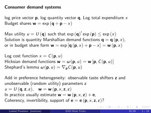
Consumer demand systems

log price vector p, log quantity vector q, Log total expenditure xBudget shares w = exp (q+ p� x)

Max utility u = U (q) such that exp (q)0 exp (p) � exp (x)Solution is quantity Marshallian demand functions q = q (p, x),or in budget share form w = exp [q (p, x) + p� x ] = w (p, x)

Log cost function x = C (p, u)Hicksian demand functions w = ω(p, u) = w [p,C (p, u)]Shephard�s lemma ω(p, u) = rpC (p, u)

Add in preference heterogeneity: observable taste shifters z andunobservable (random utility) parameters εu = U (q, z, ε), w = w (p, x , z, ε)In practice usually estimate w = w (p, x , z) + e,Coherency, invertibility, support of e = e (p, x , z, ε)?


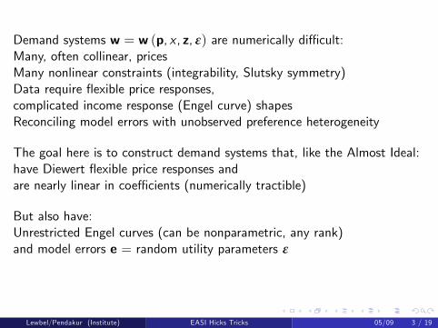
Demand systems w = w (p, x , z, ε) are numerically di¢ cult:Many, often collinear, pricesMany nonlinear constraints (integrability, Slutsky symmetry)Data require �exible price responses,complicated income response (Engel curve) shapesReconciling model errors with unobserved preference heterogeneity

The goal here is to construct demand systems that, like the Almost Ideal:have Diewert �exible price responses andare nearly linear in coe¢ cients (numerically tractible)

But also have:Unrestricted Engel curves (can be nonparametric, any rank)and model errors e = random utility parameters ε


Demand System Functional FormsCobb Douglas (1928), Geary (1951 LES) Stone (1954 LES), Arrow,Chenery, Minhas, and Solow (1961 CES), Theil (1965 Rotterdam),Armington (1969 CES), Diewert (1971 generalized leontief), Christensen,Jorgenson, and Lau (1975 translog), Howe, Pollak and Wales (1979 QES),Deaton and Muellbauer (1980 AID), Elbadawi, Gallant, and Souza (1983fourier), Banks, Blundell, Lewbel (1997 QUAIDS), Pendakur and Sperlich(2005, closest to our EASI), many others.

Engel CurvesEngel (1857, 1895), Allen and Bowley (1935), Working (1943), Leser(1963), Houthakker and Taylor (1966), Gorman (1981), Bierens andPott-Buter (1990 �rst nonparametric regression in economics?), Lewbel(1991), Blundell, Duncan and Pendakur (1998), Pendakur (1999), Koenkerand Hallock (2001 quantile), Blundell, Chen and Kristensen (2007).

Random Utility - Unobserved Taste Heterogeneity - CoherenceMcFadden and Richter (1971, 1990), Brown and Walker (1989), vanSoest, Kapteyn, and Kooreman (1993), Brown and Matzkin (1998),Lewbel (2001), Matzkin (2005), Beckert and Blundell (2008).


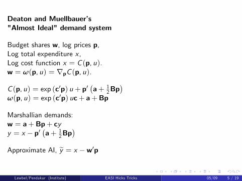
Deaton and Muellbauer�s"Almost Ideal" demand system

Budget shares w, log prices p,Log total expenditure x ,Log cost function x = C (p, u).w = ω(p, u) = rpC (p, u).

C (p, u) = exp (c0p) u + p0�a+ 1

2Bp�

ω(p, u) = exp (c0p) uc+ a+Bp

Marshallian demands:w = a+Bp+ cyy = x � p0

�a+ 1

2Bp�

Approximate AI, ey = x �w0pLewbel/Pendakur (Institute) EASI Hicks Tricks 05/09 5 / 19

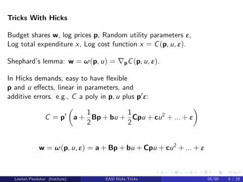
Tricks With Hicks

Budget shares w, log prices p, Random utility parameters ε,Log total expenditure x , Log cost function x = C (p, u, ε).

Shephard�s lemma: w = ω(p, u) = rpC (p, u, ε).

In Hicks demands, easy to have �exiblep and u e¤ects, linear in parameters, andadditive errors. e.g., C a poly in p, u plus p0ε:

C = p0�a+

12Bp+ bu +

12Cpu + cu2 + ...+ ε

�

w = ω(p, u, ε) = a+Bp+ bu +Cpu + cu2 + ...+ ε


Implicit Marshallian Demands

Problem with Hicks: u not observed.Solution: Implicit Marshallian Demands

The idea: construct C (p, u, ε) so thatu = g [ω(p, u, ε),p, x ] for a simple g .

Then let y = g(w,p, x) and estimateImplicit Marshallian demand functions:w = ω(p, y , ε)

In our applications y is linear in x , andy � a log money metric utility measureso will call y log real expenditures.


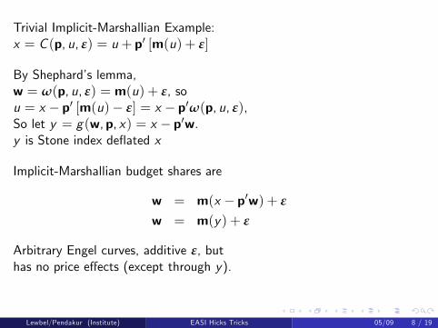
Trivial Implicit-Marshallian Example:x = C (p, u, ε) = u + p0 [m(u) + ε]

By Shephard�s lemma,w = ω(p, u, ε) = m(u) + ε, sou = x � p0 [m(u)� ε] = x � p0ω(p, u, ε),So let y = g(w,p, x) = x � p0w.y is Stone index de�ated x

Implicit-Marshallian budget shares are

w = m(x � p0w) + ε

w = m(y) + ε

Arbitrary Engel curves, additive ε, buthas no price e¤ects (except through y).


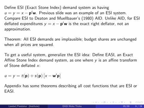
De�ne ESI (Exact Stone Index) demand system as havingu = y = x � p0w. Previous slide was an example of an ESI system.Compare ESI to Deaton and Muellbauer�s (1980) AID. Unlike AID, for ESIde�ated expenditures y = x � p0w is the exact right de�ator, not anapproximation.

Theorem: All ESI demands are implausible; budget shares are unchangedwhen all prices are squared.

To get a useful system, generalize the ESI idea: De�ne EASI, an ExactA¢ ne Stone Index demand system, as one where y is an a¢ ne transformof Stone de�ated x :

u = y = t(p) + s(p) [x �w0p]

Appendix has some theorems describing all cost functions that are ESI orEASI.


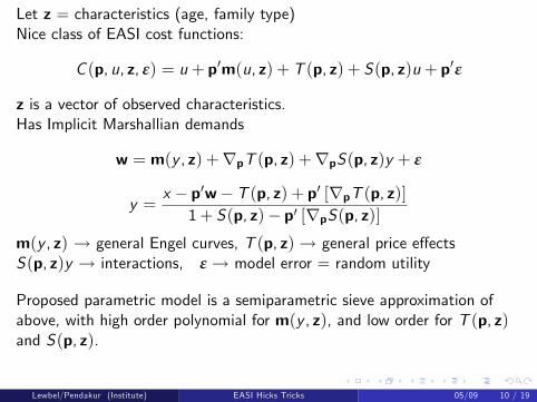
Let z = characteristics (age, family type)Nice class of EASI cost functions:

C (p, u, z, ε) = u + p0m(u, z) + T (p, z) + S(p, z)u + p0ε

z is a vector of observed characteristics.Has Implicit Marshallian demands

w = m(y , z) +rpT (p, z) +rpS(p, z)y + ε

y =x � p0w� T (p, z) + p0 [rpT (p, z)]

1+ S(p, z)� p0 [rpS(p, z)]

m(y , z) ! general Engel curves, T (p, z)! general price e¤ectsS(p, z)y ! interactions, ε ! model error = random utility

Proposed parametric model is a semiparametric sieve approximation ofabove, with high order polynomial for m(y , z), and low order for T (p, z)and S(p, z).


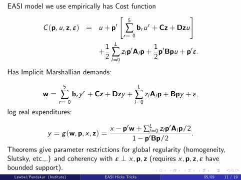
EASI model we use empirically has Cost function

C (p, u, z, ε) = u + p0"

5

∑r= 0

brur +Cz+Dzu

#

+12

L

∑l=0

zlp0Alp+12p0Bpu + p0ε.

Has Implicit Marshallian demands:

w =5

∑r= 0

br y r +Cz+Dzy +L

∑l=0

zlAlp+Bpy + ε.

log real expenditures:

y = g(w,p, x , z) =x � p0w+∑L

l=0 zlp0Alp/21� p0Bp/2

.

Theorems give parameter restrictions for global regularity (homogeneity,Slutsky, etc.,.) and coherency with ε ? x ,p, z (requires x ,p, z, ε havebounded support).


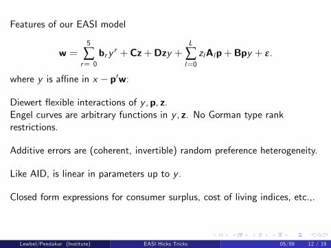
Features of our EASI model

w =5

∑r= 0

br y r +Cz+Dzy +L

∑l=0

zlAlp+Bpy + ε.

where y is a¢ ne in x � p0w:

Diewert �exible interactions of y ,p, z.Engel curves are arbitrary functions in y , z. No Gorman type rankrestrictions.

Additive errors are (coherent, invertible) random preference heterogeneity.

Like AID, is linear in parameters up to y .

Closed form expressions for consumer surplus, cost of living indices, etc.,.


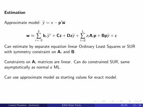
Estimation

Approximate model: ey = x � p0ww �

5

∑r= 0

brey r +Cz+Dzey + L

∑l=0

zlAlp+Bpey + ε

Can estimate by separate equation linear Ordinary Least Squares or SURwith symmetry constraint on Al and B.

Constraints on Al matrices are linear. Can do constrained SUR, sameasymptotically as normal ε ML.

Can use approximate model as starting values for exact model.


Exact model is

w =5

∑r= 0

br y r +Cz+Dzy +L

∑l=0

zlAlp+Bpy + ε

y =x � p0w+∑L

l=0 zlp0Alp/21� p0Bp/2

Use GMM (or nonlinear 3SLS) for to handle nonlinearity (one dimensional,only in y), as well as endogeneity in y and possible heteroskedasticity in ε.

Assume E (ε j x ,p, z) = 0J . Let r =(r1,...,rM )0 be bounded functions ofx ,p, z. (we let r be all the regressors in the approximate model. Then for` = 1, ...,M use E (εr`) = 0 as moments for GMM, or assuming ε ?x ,p, z, use r as 3SLS instruments.


Empirical resultsCanadian Expenditure Surveys. 12 years, 4 regions, in 1969 to 1999.urban, rental-tenure, singles. 4,847 observations, 48 price regimes.

9 Categories:food-in, food-out, rent, clothing, household operation, householdfurnishing & equipment, transport operation, recreation, personal care.

z is age, sex, car dummy, social assistance dummy, time.Also, numerically scale y so y5 is ok.

Tables and Figures at the end of these slides. Summarize some highlightsfor now.


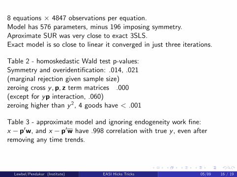
8 equations � 4847 observations per equation.Model has 576 parameters, minus 196 imposing symmetry.Aproximate SUR was very close to exact 3SLS.Exact model is so close to linear it converged in just three iterations.

Table 2 - homoskedastic Wald test p-values:Symmetry and overidenti�cation: .014, .021(marginal rejection given sample size)zeroing cross y ,p, z term matrices .000(except for yp interaction, .060)zeroing higher than y2, 4 goods have < .001

Table 3 - approximate model and ignoring endogeneity work �ne:x � p0w, and x � p0w have .998 correlation with true y , even afterremoving any time trends.


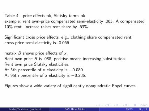
Table 4 - price e¤ects ok, Slutsky terms ok.example: rent own-price compensated semi-elasticity .063. A compensated10% rent increase raises rent share by .63%

Signi�cant cross price e¤ects, e.g., clothing share compensated rentcross-price semi-elasticity is -0.066

matrix B shows price e¤ects of x .Rent own-price B is .088, positive means increasing substitution.Rent own price Slutsky elasticities:At 5th percentile of x elasticity is �0.080.At 95th percentile of x elasticity is �0.236.

Figures show a wide variety of signi�cantly nonquadratic Engel curves.


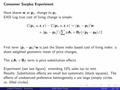
Consumer Surplus Experiment

Have shares w at p0, change to p1.EASI Log true cost of living change is simple:

C (p1, u, z, ε)� C (p0, u, z, ε) = (p1 � p0)0w+ (p1 � p0)0

�∑ zlAl +By

�(p1 � p0)/2

First term (p1 � p0)0w is just the Stone index based cost of living index: ashare weighted geometric mean of price changes.

The zlAl +By term is price substitution e¤ects

Experiment (see last �gure): extending 15% sales tax to rent.Results: Substitution e¤ects are small but systematic (black squares). Thee¤ects of unobserved preference heterogeneity ε are large (empty circlesvs. �lled circles).


Additional Results in the paper

Closed form Marshallian and Hicksian elasticity expressions.

Consumer Surplus theory

Existence of general y = g(x ,w,p).

Global regularity conditions.

Coherence and invertibility of ε.

Closure Under Unit Scaling.

Conditions for Shape Invariance.

Properties of associated indirect utility and Marshallian demands.


Table 1: Data Descriptives

Variable Mean Std Dev Minimum Maximum

budget shares Food-at-Home 0.14 0.08 0.00 0.61Food-Out 0.08 0.07 0.00 0.63

Rent 0.37 0.12 0.01 0.89

Household Oper 0.07 0.04 0.00 0.61Household Furneq 0.04 0.05 0.00 0.52

Clothing 0.08 0.06 0.00 0.48

Transport Oper 0.11 0.08 0.00 0.60Recreation 0.08 0.07 0.00 0.59Personal Care 0.03 0.02 0.00 0.21

log-prices Food-at-Home -0.05 0.43 -1.41 0.34Food-Out 0.04 0.49 -1.46 0.53Rent -0.08 0.40 -1.27 0.37Household Oper -0.06 0.45 -1.40 0.32Household Furneq -0.05 0.32 -0.94 0.20Clothing 0.04 0.35 -0.94 0.34Transport Oper -0.07 0.57 -1.53 0.57Recreation 0.01 0.40 -1.04 0.42Personal Care -0.03 0.38 -1.11 0.29

demographics age-40 0.71 11.89 -15.00 24.00male 0.51 0.50 0.00 1.00

car-owner 0.42 0.49 0.00 1.00social asst 0.27 0.44 0.00 1.00time 88.99 8.73 69.00 99.00

log-expenditure x -0.11 0.59 -2.75 1.66(median-norm'd) x- p'w -0.07 0.44 -1.70 1.44

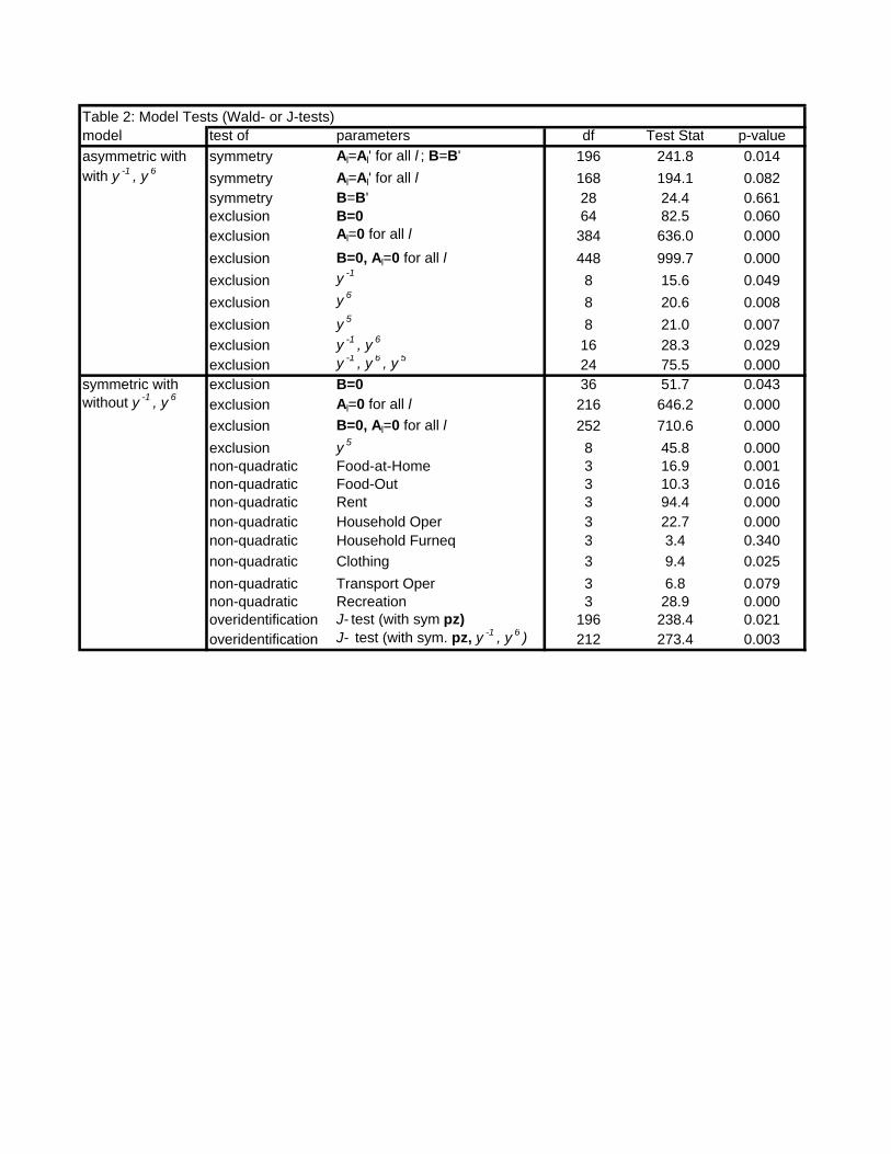
Table 2: Model Tests (Wald- or J-tests)model test of parameters df Test Stat p-valueasymmetric with symmetry Al=Al' for all l ; B=B' 196 241.8 0.014with y -1 , y 6

symmetry Al=Al' for all l 168 194.1 0.082symmetry B=B' 28 24.4 0.661exclusion B=0 64 82.5 0.060exclusion Al=0 for all l 384 636.0 0.000

exclusion B=0, Al=0 for all l 448 999.7 0.000

exclusion y -18 15.6 0.049

exclusion y 68 20.6 0.008

exclusion y 5 8 21.0 0.007exclusion y -1 , y 6 16 28.3 0.029exclusion y -1 , y 6 , y 5

24 75.5 0.000symmetric with exclusion B=0 36 51.7 0.043without y -1 , y 6

exclusion Al=0 for all l 216 646.2 0.000exclusion B=0, Al=0 for all l 252 710.6 0.000

exclusion y 5 8 45.8 0.000non-quadratic Food-at-Home 3 16.9 0.001non-quadratic Food-Out 3 10.3 0.016non-quadratic Rent 3 94.4 0.000non-quadratic Household Oper 3 22.7 0.000non-quadratic Household Furneq 3 3.4 0.340non-quadratic Clothing 3 9.4 0.025

non-quadratic Transport Oper 3 6.8 0.079non-quadratic Recreation 3 28.9 0.000overidentification J- test (with sym pz) 196 238.4 0.021overidentification J- test (with sym. pz, y -1 , y 6 ) 212 273.4 0.003

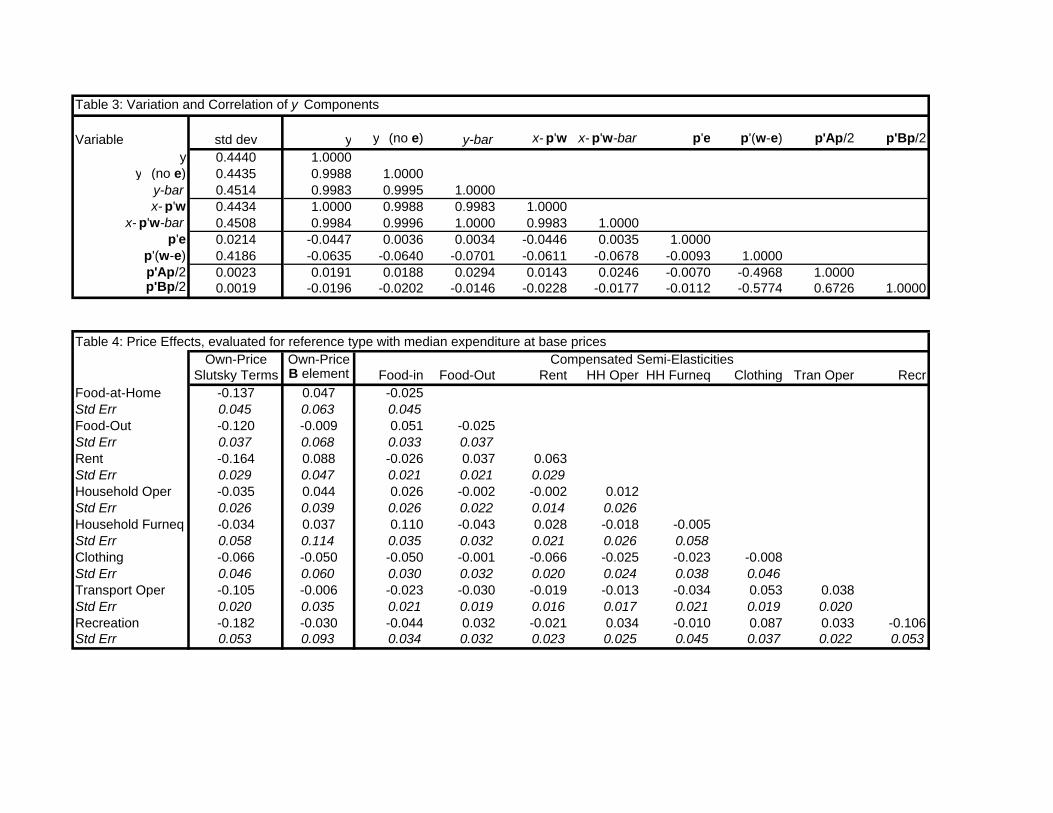
Table 3: Variation and Correlation of y Components

Variable std dev y y (no e) y-bar x- p'w x- p'w-bar p'e p'(w-e) p'Ap/2 p'Bp/2y 0.4440 1.0000

y (no e) 0.4435 0.9988 1.0000y-bar 0.4514 0.9983 0.9995 1.0000x- p'w 0.4434 1.0000 0.9988 0.9983 1.0000

x- p'w-bar 0.4508 0.9984 0.9996 1.0000 0.9983 1.0000p'e 0.0214 -0.0447 0.0036 0.0034 -0.0446 0.0035 1.0000

p'(w-e) 0.4186 -0.0635 -0.0640 -0.0701 -0.0611 -0.0678 -0.0093 1.0000p'Ap/2 0.0023 0.0191 0.0188 0.0294 0.0143 0.0246 -0.0070 -0.4968 1.0000p'Bp/2 0.0019 -0.0196 -0.0202 -0.0146 -0.0228 -0.0177 -0.0112 -0.5774 0.6726 1.0000

Table 4: Price Effects, evaluated for reference type with median expenditure at base pricesOwn-Price Own-Price

Slutsky Terms B element Food-in Food-Out Rent HH Oper HH Furneq Clothing Tran Oper RecrFood-at-Home -0.137 0.047 -0.025Std Err 0.045 0.063 0.045Food-Out -0.120 -0.009 0.051 -0.025Std Err 0.037 0.068 0.033 0.037Rent -0.164 0.088 -0.026 0.037 0.063Std Err 0.029 0.047 0.021 0.021 0.029Household Oper -0.035 0.044 0.026 -0.002 -0.002 0.012Std Err 0.026 0.039 0.026 0.022 0.014 0.026Household Furneq -0.034 0.037 0.110 -0.043 0.028 -0.018 -0.005Std Err 0.058 0.114 0.035 0.032 0.021 0.026 0.058Clothing -0.066 -0.050 -0.050 -0.001 -0.066 -0.025 -0.023 -0.008Std Err 0.046 0.060 0.030 0.032 0.020 0.024 0.038 0.046Transport Oper -0.105 -0.006 -0.023 -0.030 -0.019 -0.013 -0.034 0.053 0.038Std Err 0.020 0.035 0.021 0.019 0.016 0.017 0.021 0.019 0.020Recreation -0.182 -0.030 -0.044 0.032 -0.021 0.034 -0.010 0.087 0.033 -0.106Std Err 0.053 0.093 0.034 0.032 0.023 0.025 0.045 0.037 0.022 0.053

Compensated Semi-Elasticities

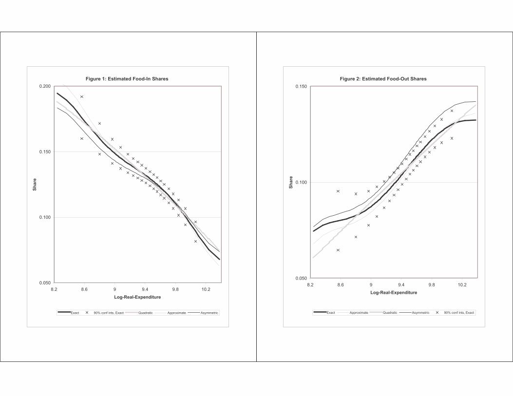
Figure 1: Estimated Food-In Shares

0.050

0.100

0.150

0.200

8.2 8.6 9 9.4 9.8 10.2

Log-Real-Expenditure

Sh

are

Exact 90% conf ints, Exact Quadratic Approximate Asymmetric

Figure 2: Estimated Food-Out Shares

0.050

0.100

0.150

8.2 8.6 9 9.4 9.8 10.2

Log-Real-ExpenditureS

har

e

Exact Approximate Quadratic Asymmetric 90% conf ints, Exact

Figure 3: Estimated Rent Shares

0.200

0.250

0.300

0.350

0.400

8.2 8.6 9 9.4 9.8 10.2


Sh

are

Exact Quadratic 90% conf ints, Exact Asymmetric Approximate

Figure 4: Estimated Household Operation Shares

0.04

0.05

0.06

0.07

0.08

0.09

8.2 8.6 9 9.4 9.8 10.2


Sh

are

Exact Quadratic Asymmetric 90% conf ints, Exact Approximate

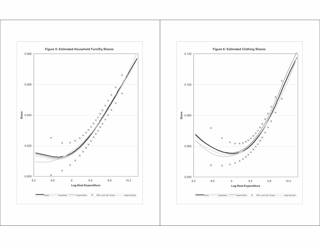
Figure 5: Estimated Household Furn/Eq Shares

0.000

0.020

0.040

0.060

0.080

8.2 8.6 9 9.4 9.8 10.2


Sh

are


Figure 6: Estimated Clothing Shares

0.040

0.060

0.080

0.100

0.120

8.2 8.6 9 9.4 9.8 10.2


Sh

are


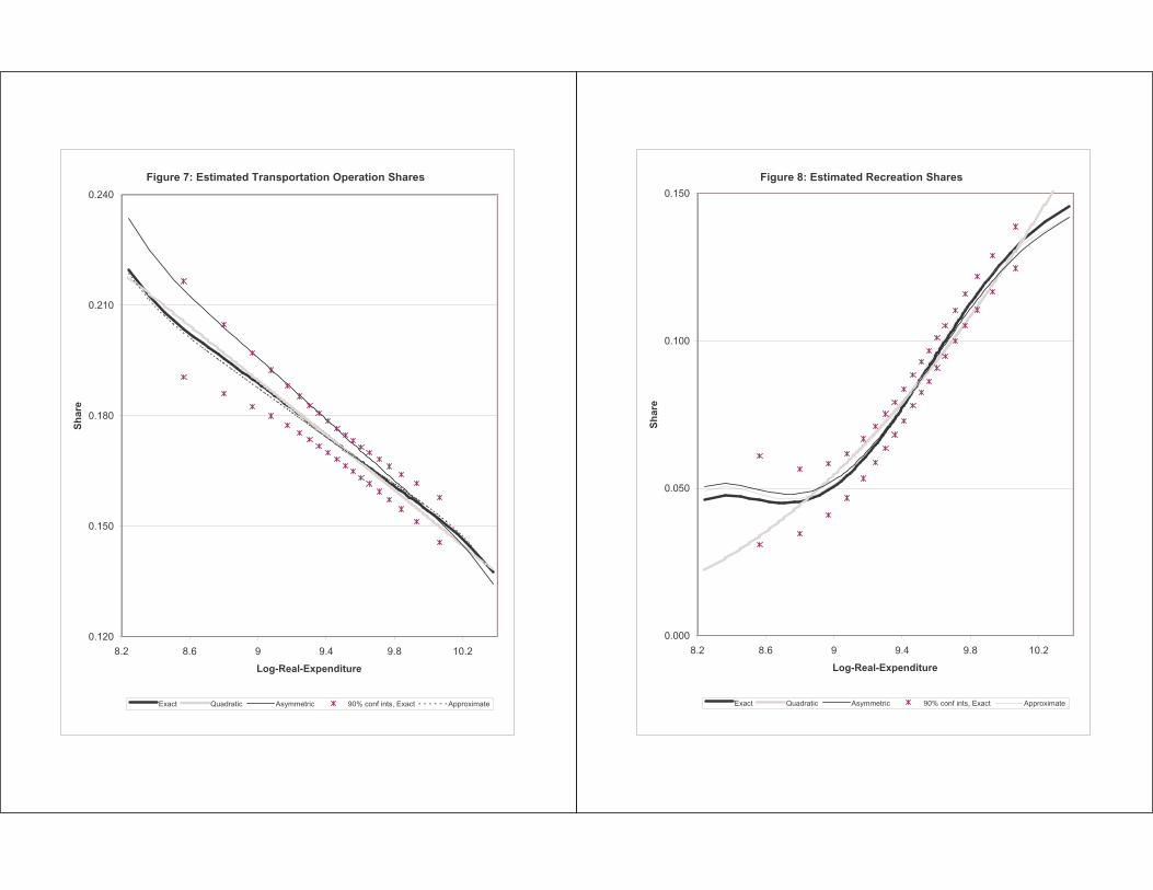
Figure 7: Estimated Transportation Operation Shares

0.120

0.150

0.180

0.210

0.240

8.2 8.6 9 9.4 9.8 10.2


Sh

are


Figure 8: Estimated Recreation Shares

0.000

0.050

0.100

0.150

8.2 8.6 9 9.4 9.8 10.2


Sh

are


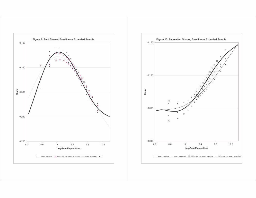
Figure 9: Rent Shares: Baseline vs Extended Sample

0.200

0.250

0.300

0.350

0.400

8.2 8.6 9 9.4 9.8 10.2


Sh

are

exact, baseline 90% conf ints, exact, extended exact, extended

Figure 10: Recreation Shares, Baseline vs Extended Sample

0.000

0.050

0.100

0.150

8.2 8.6 9 9.4 9.8 10.2


Sh

are

exact, baseline exact, extended 90% conf ints, exact, baseline 90% conf ints, exact, extended

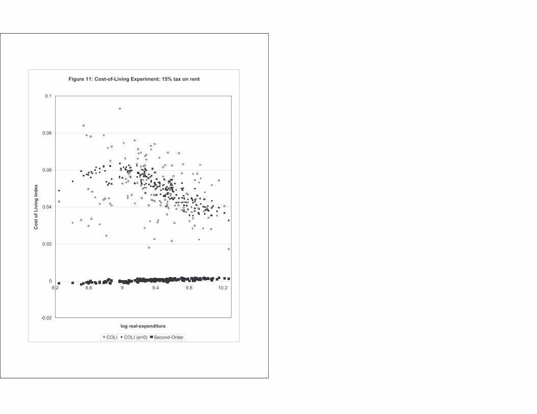
Figure 11: Cost-of-Living Experiment: 15% tax on rent

-0.02

0

0.02

0.04

0.06

0.08

0.1

8.2 8.6 9 9.4 9.8 10.2

log real-expenditure

Co

st o

f L

ivin

g In

dex

COLI COLI (e=0) Second-Order

tricks with hicks: the easi demand system - bc.edu · tricks with hicks: the easi demand system ......

Documents