Tricks With Hicks: The EASI Demand System

Arthur Lewbel and Krishna PendakurBoston College and Simon Fraser University

Revised March 2008

Abstract

We invent Implicit Marshallian Demands, a new type of demand function that combinesdesirable features of Hicksian and Marshallian demand functions. We propose and estimatethe Exact Af�ne Stone Index (EASI) Implicit Marshallian Demand system. Like the AlmostIdeal Demand (AID) system, EASI budget shares are linear in parameters given real expendi-tures. However, unlike the AID, EASI demands can have any rank and its Engel curves canbe polynomials or splines of any order in real expenditures. EASI error terms equal randomutility parameters to account for unobserved preference heterogeneity. EASI demand functionscan be estimated using GMM or three stage least squares, and, like AID, an approximate EASImodel can be estimated by linear regression.

JEL Codes: D11, D12, C31, C33, C51

Keywords: Consumer demand, Demand systems, Hicks, Marshallian, Cost functions, Expenditure func-

tions, Utility, Engel curves.

The authors wish to thank Richard Blundell, Angus Deaton, David Donaldson, Stefan Sperlich, and many

anonymous referees for helpful comments. Any errors are our own.

1

1 Introduction

Recent empirical work with large consumer expenditure data sets �nds Engel curves (income ex-pansion paths) with signi�cant curvature and variation across goods. For example, some goodshave Engel curves that are close to linear or quadratic, while others are more S-shaped (see, Blun-dell, Chen and Kristensen (2007). Typical parametric demand models cannot encompass this vari-ety of shapes, and are constrained by Gorman (1981) type rank restrictions.Other current research shows the importance of allowing for unobserved preference hetero-

geneity in demand systems, and the dif�culty of doing so in a coherent fashion. In most empiricalmodels of consumer demand, model error terms cannot be interpreted as random utility parametersrepresenting unobserved heterogeneity. See, for example, Brown and Walker (1989), McFaddenand Richter (1990), Brown and Matzkin (1998), Lewbel (2001), and Beckert and Blundell (2004).Despite these empirical issues, Deaton and Muellbauer's (1980) Almost Ideal Demand (AID)

model, which has linear Engel curves and does not incorporate unobserved heterogeneity, remainsvery popular. This popularity is at least partly because alternative models involve nonlinear func-tions of many prices and parameters, which are often numerically dif�cult or intractible to imple-ment. In addition, the AID model has a very convenient approximate form which may be estimatedby linear methods.In this paper, we develop an approach to the speci�cation and estimation of consumer demands

that addresses the above issues while maintaining the simplicity of the AID model. Considera consumer with demographic (and other observable preference related) characteristics z and lognominal total expenditures x that faces the J�vector of log prices p. Assume she chooses a bundleof goods, described by the J� vector of budget shares w, to maximize utility given her linearbudget constraint. Hicksian demand functions associated with her utility function, which expressw as a function of p, z, and attained utility level u, can easily be speci�ed to have many desirableproperties. We show that under some conditions, which permit both random utility parametersand arbitrarily complicated Engel curves, utility u can be expressed as a simple function of theobserved variables x , w, p, and z. This function, which we denote y, can often be interpreted asa measure of log real expenditures. We use these results to directly specify and estimate what wecall implicit Marshallian demands, which are Hicksian demands after replacing u with the implicitutility measure y.Noting that p0w is the de�nition of the Stone (1954) log price index, we de�ne the Exact

Af�ne Stone Index (EASI) class of cost functions, which have y equal to an af�ne transform ofStone index de�ated log nominal expenditures, x � p0w. The resulting EASI implicit Marshalliandemand functions have the following properties:1. Like the AID system, EASI budget share demand functions are, apart from the construction

2

of y, completely linear in parameters, which facilitates estimation in models with many goods.2. The AID budget shares are linear in p, z, and y. In contrast, EASI budget shares are linear

in p and are polynomials of any order in z and y. They can also include interaction terms such aspy, zy and pz0, and contain other functions of z and y.3. EASI Engel curves for each good are almost completely unrestricted. For example, EASI

demands can be high order polynomials or splines in y and z, and so can encompass empiricallyimportant speci�cations that most parametric models cannot capture, such as the semiparametricS shaped Engel curves reported by Pendakur (1999) and Blundell, Chen and Kristensen (2007).The AID system is linear in y and has rank two, and the quadratic AID of Banks, Blundell, andLewbel (1997) is quadratic in (an approximation of) y with rank three. In contrast, EASI demandscan be polynomials or splines of any order in y, and can have any rank up to J-1, where J is thenumber of goods. EASI demands are not subject to the Gorman (1981) rank three limit even withpolynomial Engel curves (see the Appendix for de�nitions and details regarding the meaning andnature of rank restrictions).4. EASI budget share error terms can equal unobserved preference heterogeneity or random

utility parameters. The AID and other similar models do not have this property, since in thosemodels unobserved preference heterogeneity requires that additive errors be heteroskedastic (seeBrown and Walker 1989 and Lewbel 2001). The EASI unobserved preference heterogeneity iscoherent and invertible (see the Appendix).5. EASI demand functions can be estimated using nonlinear instrumental variables, particularly

nonlinear three-stage least-squares (3SLS) and Hansen's (1982) Generalized Method of Moments(GMM). Like the AID system, approximate versions of EASI demands can be estimated by linearregression. We �nd little empirical difference between exact nonlinear and approximate linearEASI estimates.6. Since EASI demands are derived from a cost function model, given estimated parameters

we have simple closed form expressions for consumer surplus calculations, such as cost-of-livingindices for large price changes.EASI demands thus accomodate an extremely wide class of functional forms. In the empirical

work below, we implement a model where, for the budget share w j of each good j , the estimatingequations for demand system have the linear in parameters form

w j D5XrD0br j yr C

LXlD1

�Cl j zl C Dl j zl y

�CC

LXlD0

JXkD1

Alk j zl pk CJXkD1

Bk j pk y C " j ,

where y is a measure of real total expenditures. The regressors in this model are a �fth orderpolynomial in y, log-prices pk of each good k, and L different demographic characteristics zl ,in addition to interaction terms of the forms pk y, zl y, and zl pk . Our approximate EASI model

3

estimates these equations for each good j by ordinary least squares, letting y equal x�PJ

jD1 p jw j ,while the exact model has y given by equation (8) below.We begin with an overview of our approach, de�ning implicit Marshallian demand functions

and general EASI demands. We show how these models accomodate high rank engel curves andunobserved preference heterogeneity. We describe the speci�c EASI functional form we will usein our empirical application, and also show how to construct a fully linear approximation for ourEASI demand model, analogous to the approximate linear AID model. We show how to apply theEASI model with consumer surplus and compensated elasticity calculations. Then we describeestimators for the EASI model, including consistent, asymptotically normal instrumental variable,three stage least squares, and GMM estimators for the exact model and linear least squares estima-tors for the approximate model.We estimate the exact model using Canadian micro-data. We �nd more complicated Engel

curve shapes than those of standard parametric demand systems, and we �nd that the simple ap-proximate EASI model captures this complexity very well. We apply the model to a cost-of-livingexperiment, and �nd that both the increased �exibility of Engel curves and the incorporation ofunobserved heterogeneity into the model signi�cantly affect the resulting welfare calculations.An appendix provides formal theorems and proofs, along with some extensions and additional

mathematical properties of EASI and other implicit Marshallian demands, which are relevant forevaluating these models and for other possible applications of our general methodology.

2 Methods and Models

Here we de�ne the general idea of implicit Marshallian demands, describe the EASI functionalform, and explain how this model can be estimated and applied. Formal theorems regarding thesemethods and models are provided in the Appendix.

2.1 Implicit Marshallian Demand Functions

We specify a cost (expenditure) function and use Shephard's lemma to obtain Hicksian demandsthat have the desired properties. The usual next step would be to obtain Marshallian demands,which are functions of p, z and x , by solving for indirect utility u in terms of p, z and x , andsubstituting this into Hicksian demand functions. We instead construct cost functions that havesimple expressions for u in terms of w, p, z and x . We call this expression y, implicit utility,and substitute y for u in the Hicksian demands to yield what we call implicit Marshallian demandfunctions. These implicit Marshallian demands circumvent the dif�culty of �nding simple analyticexpressions for indirect utility or Marshallian demands.

4

We wish to explicitly include both observable and unobservable sources of preference hetero-geneity in our models, so let z D .z1; :::; zL/0 be an L�vector of observable demographic (or other)characteristics that affect preferences, and let " be a J�vector of unobserved preference charac-teristics (taste parameters) satisfying 10J" D 0 where 1J is the J�vector of ones. Typical elementsof z would include household size, age, and composition. The log cost or expenditure function isx D C.p; u; z; "/, which equals the minimum log-expenditure required for an individual with char-acteristics z; " to attain utility level u when facing log prices p. Sheppard's Lemma expresses Hick-sian (compensated) budget-share functions, !.p; u; z; "/, as w D !.p; u; z; "/ D rpC.p; u; z; "/.Indirect utility, V , is the inverse of log-cost with respect to u: u D V .p; x; z; "/ D C�1.p; �; z; "/.If an analytic solution for V is unavailable, it may still be possible to express utility as a functiong of w;p; x; z. In this case, we can write u D g.!.p; u; z; "/;p; x; z/, which implicitly de�nesu. We may then de�ne implicit utility y by y D g.w;p; x; z/. By construction, y D u and thefunction g that de�nes y depends only on observable data, and may have a simple tractible closedform expression even when no closed form expression exists for indirect utility V . The implicitMarshallian demand system is then given by w D !.p; y; z; "/, which is the Hicksian demandsystem except for replacing u with y.A similar idea to implicit marshallian demands is Browning's (2001) `M-demands,' which

expresses demand functions in terms of prices and the quantity of one good, instead of in terms ofprices and total expenditures. This can be interpreted as a restrictive choice of g, since it uses onlyone good.In this construction, preferences and hence utility remain ordinal. So when we say that im-

plicit utility y equals the utility level u, this only means that the observable y equals one possiblecardinalization of u. In all our examples y will be linear in x and will either equal or closelyapproximate a money metric cardinalization of utility, and hence y will also be interpretable asa measure of real expenditures. We will sometimes refer to y as log real expenditures when thisinterpretation of implicit utility is particularly relevant.Since g expresses utility as a function of all the arguments of indirect utility plus allowing

for dependence !, it admits more possiblities than are available for explicit marshallian demandsystems. Although, in theory, the idea of implicit demand systems opens up an extremely largeclass of potential demand systems, we �nd that simple forms for g allow us to solve a large numberof problems facing empirical demand analysis.Just to illustrate the idea of implicit Marshallian demands, consider the following restrictive

example. For simplicity (ignoring the inequality constraints required for demand system regularity)consider a log cost function of the form

C.p; u; z; "/ D u C p0m.u; z/C p0" (1)

5

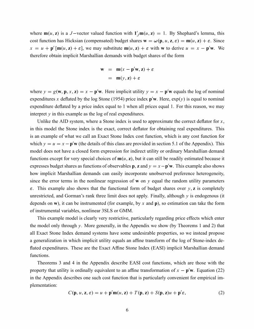
where m.u; z/ is a J�vector valued function with 10Jm.u; z/ D 1. By Shephard's lemma, thiscost function has Hicksian (compensated) budget shares w D !.p; u; z; "/ D m.u; z/ C ". Sincex D u C p0 [m.u; z/C "], we may substitute m.u; z/ C " with w to derive u D x � p0w. Wetherefore obtain implicit Marshallian demands with budget shares of the form

w D m.x � p0w; z/C "

D m.y; z/C "

where y D g.w;p; x; z/ D x � p0w. Here implicit utility y D x � p0w equals the log of nominalexpenditures x de�ated by the log Stone (1954) price index p0w. Here, exp.y/ is equal to nominalexpenditure de�ated by a price index equal to 1 when all prices equal 1. For this reason, we mayinterpret y in this example as the log of real expenditures.Unlike the AID system, where a Stone index is used to approximate the correct de�ator for x ,

in this model the Stone index is the exact, correct de�ator for obtaining real expenditures. Thisis an example of what we call an Exact Stone Index cost function, which is any cost function forwhich y D u D x�p0w (the details of this class are provided in section 5.1 of the Appendix). Thismodel does not have a closed form expression for indirect utility or ordinary Marshallian demandfunctions except for very special choices ofm.u; z/, but it can still be readily estimated because itexpresses budget shares as functions of observables p; z and y D x�p0w. This example also showshow implicit Marshallian demands can easily incorporate unobserved preference heterogeneity,since the error terms in the nonlinear regression of w on y equal the random utility parameters". This example also shows that the functional form of budget shares over y; z is completelyunrestricted, and Gorman's rank three limit does not apply. Finally, although y is endogenous (itdepends on w), it can be instrumented (for example, by x and p), so estimation can take the formof instrumental variables, nonlinear 3SLS or GMM.This example model is clearly very restrictive, particularly regarding price effects which enter

the model only through y. More generally, in the Appendix we show (by Theorems 1 and 2) thatall Exact Stone Index demand systems have some undesirable properties, so we instead proposea generalization in which implicit utility equals an af�ne transform of the log of Stone-index de-�ated expenditures. These are the Exact Af�ne Stone Index (EASI) implicit Marshallian demandfunctions.Theorems 3 and 4 in the Appendix describe EASI cost functions, which are those with the

property that utility is ordinally equivalent to an af�ne transformation of x � p0w. Equation (22)in the Appendix describes one such cost function that is particularly convenient for empirical im-plementation:

C.p; u; z; "/ D u C p0m.u; z/C T .p; z/C S.p; z/u C p0"; (2)

6

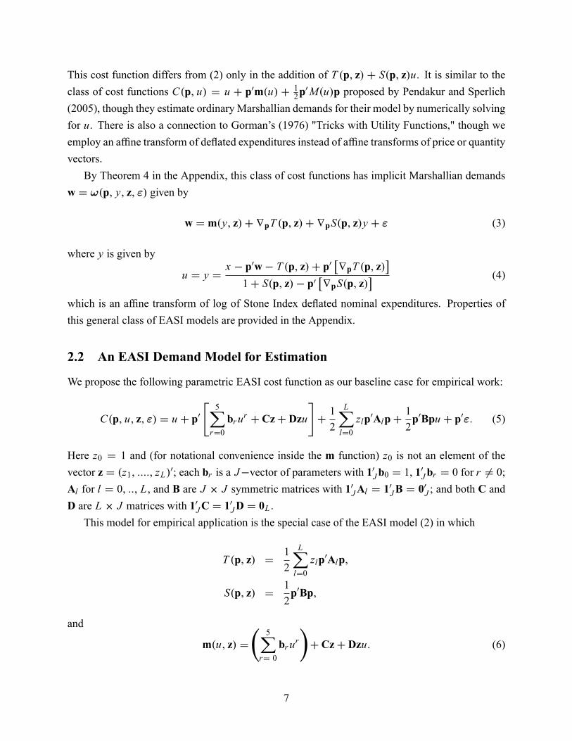
This cost function differs from (2) only in the addition of T .p; z/ C S.p; z/u. It is similar to theclass of cost functions C.p; u/ D u C p0m.u/ C 1

2p0M.u/p proposed by Pendakur and Sperlich

(2005), though they estimate ordinary Marshallian demands for their model by numerically solvingfor u. There is also a connection to Gorman's (1976) "Tricks with Utility Functions," though weemploy an af�ne transform of de�ated expenditures instead of af�ne transforms of price or quantityvectors.By Theorem 4 in the Appendix, this class of cost functions has implicit Marshallian demands

w D !.p; y; z; "/ given by

w D m.y; z/CrpT .p; z/CrpS.p; z/y C " (3)

where y is given by

u D y Dx � p0w� T .p; z/C p0

�rpT .p; z/

�1C S.p; z/� p0

�rpS.p; z/

� (4)

which is an af�ne transform of log of Stone Index de�ated nominal expenditures. Properties ofthis general class of EASI models are provided in the Appendix.

2.2 An EASI Demand Model for Estimation

We propose the following parametric EASI cost function as our baseline case for empirical work:

C.p; u; z; "/ D u C p0"5XrD0brur C CzC Dzu

#C12

LXlD0zlp0AlpC

12p0Bpu C p0": (5)

Here z0 D 1 and (for notational convenience inside the m function) z0 is not an element of thevector z D .z1; ::::; zL/0; each br is a J�vector of parameters with 10Jb0 D 1, 1

0Jbr D 0 for r 6D 0;

Al for l D 0; ::; L , and B are J � J symmetric matrices with 10JAl D 10JB D 0

0J ; and both C and

D are L � J matrices with 10JC D 10JD D 0L .

This model for empirical application is the special case of the EASI model (2) in which

T .p; z/ D12

LXlD0zlp0Alp;

S.p; z/ D12p0Bp;

and

m.u; z/ D

5X

rD 0brur

!C CzC Dzu: (6)

7

The vector of functionsm.u; z/, which generates the model's Engel curves, could be replaced withother sets of �exible functions of u; z such as splines. We use a polynomial in u and an af�nefunction of z to strike a balance between simple tractability and general Engel curve �exibility. Wechoose quadratic forms in prices for T and S because these have simple gradient vectorsrpT .p; z/and rpS.p; z/. Finally, we make S independent of z for the sake of terseness.By Shephard's lemma, the cost function (5) has Hicksian (compensated) budget shares

w D5XrD0brur C CzC Dzu C

LXlD0zlAlpC Bpu C " (7)

It can be readily checked from these formulas that

C.p; u; z; "/ D u C p0w�LXlD0zlp0Alp=2� p0Bpu=2;

and solving this expression for u yields implicit utility y:

y D g.w;p; x; z/ Dx � p0wC

PLlD0 zlp0Alp=2

1� p0Bp=2: (8)

This y has many of the properties of log real expenditures. It equals a cardinalization of utilityu, it is af�ne in nominal expenditures x , and it equals x in the base period when all prices equalone (which is when log prices p equal zero). Also, when B is zero, y exactly equals the log ofnominal expenditures de�ated by a price index. We later show empirically that y is very highlycorrelated with the log of stone index de�ated nominal expenditures, which is a very popular ad hocmeasure of real expenditures. Like any money-metric utility measure, y is just a mathematicallyconvenient representation of utility and need not have any deeper signi�cance as an objective orinterpersonally comparable utility measure (see the "Shape Invariance and Equivalence Scales"section in the Appendix for details).Substituting implicit utility y into the Hicksian budget shares yields the implicit Marshallian

budget shares

w D5XrD0br yr C CzC Dzy C

LXlD0zlAlpC Bpy C ": (9)

which is the matrix form of the equation provided in the introduction.Given y, which is a function of observables x , p, z and the log Stone index p0w, the bud-

get share equations (9) are linear in parameters and so can be easily estimated. An approximateestimator applies ordinary (linear) least squares after replacing y with x � p0w in (9), just likeestimation of the approximate AID model. Better estimators simultaneously estimate the model

8

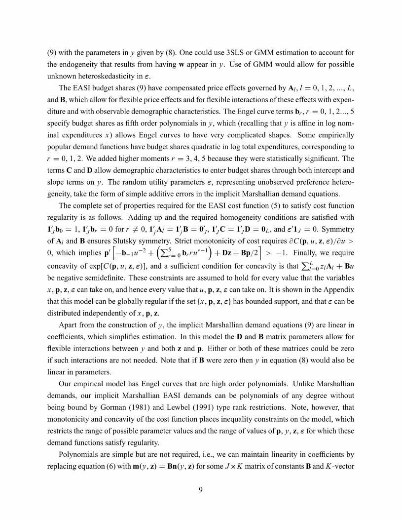
(9) with the parameters in y given by (8). One could use 3SLS or GMM estimation to account forthe endogeneity that results from having w appear in y. Use of GMM would allow for possibleunknown heteroskedasticity in ".The EASI budget shares (9) have compensated price effects governed by Al , l D 0; 1; 2; :::; L ,

andB, which allow for �exible price effects and for �exible interactions of these effects with expen-diture and with observable demographic characteristics. The Engel curve terms br , r D 0; 1; 2:::; 5specify budget shares as �fth order polynomials in y, which (recalling that y is af�ne in log nom-inal expenditures x) allows Engel curves to have very complicated shapes. Some empiricallypopular demand functions have budget shares quadratic in log total expenditures, corresponding tor D 0; 1; 2. We added higher moments r D 3; 4; 5 because they were statistically signi�cant. Theterms C and D allow demographic characteristics to enter budget shares through both intercept andslope terms on y. The random utility parameters ", representing unobserved preference hetero-geneity, take the form of simple additive errors in the implicit Marshallian demand equations.The complete set of properties required for the EASI cost function (5) to satisfy cost function

regularity is as follows. Adding up and the required homogeneity conditions are satis�ed with10Jb0 D 1, 1

0Jbr D 0 for r 6D 0, 1

0jAl D 1

0jB D 0

0J , 1

0JC D 1

0JD D 0L , and "

01J D 0. Symmetryof Al and B ensures Slutsky symmetry. Strict monotonicity of cost requires @C.p; u; z; "/=@u >0, which implies p0

h�b�1u�2 C

�P5rD 0 brrur�1

�C DzC Bp=2

i> �1. Finally, we require

concavity of exp[C.p; u; z; "/], and a suf�cient condition for concavity is thatPLlD0 zlAl C Bu

be negative semide�nite. These constraints are assumed to hold for every value that the variablesx;p; z; " can take on, and hence every value that u;p; z; " can take on. It is shown in the Appendixthat this model can be globally regular if the set fx;p; z; "g has bounded support, and that " can bedistributed independently of x;p; z.Apart from the construction of y, the implicit Marshallian demand equations (9) are linear in

coef�cients, which simpli�es estimation. In this model the D and B matrix parameters allow for�exible interactions between y and both z and p. Either or both of these matrices could be zeroif such interactions are not needed. Note that if B were zero then y in equation (8) would also belinear in parameters.Our empirical model has Engel curves that are high order polynomials. Unlike Marshallian

demands, our implicit Marshallian EASI demands can be polynomials of any degree withoutbeing bound by Gorman (1981) and Lewbel (1991) type rank restrictions. Note, however, thatmonotonicity and concavity of the cost function places inequality constraints on the model, whichrestricts the range of possible parameter values and the range of values of p; y; z; " for which thesedemand functions satisfy regularity.Polynomials are simple but are not required, i.e., we can maintain linearity in coef�cients by

replacing equation (6) withm.y; z/ D Bn.y; z/ for some J�K matrix of constantsB and K -vector

9

of known functions n.y; z/. Our chosen functional form takes n.y; z/ to be a vector of elementsof the form ur and ur zl , but other functions could also be chosen. For example, the elementsof n.y; z/ could be splines or bounded functions such as logistic transformations of polynomials(which would automatically bound estimated budget shares). Semiparametric speci�cations couldbe obtained by letting n.y; z/ be basis functions with the number of elements of n growing toin�nity with sample size.

2.3 Approximate Fully Linear Model

The demand functions (9) are linear in parameters except for the termsPLlD0 zlp0Alp and p0Bp that

appear in the construction of y in (8). A similar nonlinearity appears in Deaton and Muellbauer's(1980) AID system and Banks, Blundell, and Lewbel's (1997) QUAID system, and can be dealtwith in an analogous way, either by nonlinear estimation or by replacing y with an observable ap-proximation. Consider approximating our real expenditures measure y with nominal expendituresde�ated by a Stone price index, that is, replace y withey de�ned by

ey D x � p0w (10)

for some set of budget shares w. Then by comparison with equation (9) we have

w D5XrD0breyr C CzC Dzey C LX

lD0zlAlpC Bpey Ce" (11)

wheree" � " withe" de�ned to make equations (11) hold. We call the model of equations (10) and(11) the Approximate EASI model.The Approximate EASI nests the model w D b0 C b1ey C Cz C Ap Ce", which is identical to

the popular approximate Almost Ideal Demand System (AID) if ey D x � p0w (that is, w D w).The AID without the approximation has y equal to de�ated x where the log de�ator is quadratic inp, while the EASI model without approximation has y equal to an af�ne transform of x � p0w.The approximate EASI also nests the model w D b0 C b1ey C b2ey2 C Cz C Ap Ce", which is

the model estimated by Blundell, Pashardes, and Weber (1993). Their motivation for this modelwas by analogy with the Almost Ideal, but if this model was really to be Marshallian then, as theyshow, utility maximization would require linear rank restrictions on the coef�cients b0, b1, and b2,which they did not impose. The approximate EASI implicit Marshallian demand function there-fore provides a rationale for the unrestricted model that Blundell, Pashardes, and Weber actuallyestimated.The approximate EASI model, substituting equation (10) into (11), can be estimated by linear

10

regression methods, with linear cross-equation symmetry restrictions on the Al and B coef�cients.A natural choice for w is the sample average of budget shares across consumers. A better ap-proximation to y would be to let w be each consumer's own w, so each consumer has their ownStone index de�ator based on their own budget shares. However, as discussed later, this betterapproximation introduces endogeneity.In our empirical application, we estimate the approximate model with w D w using seem-

ingly unrelated regressions, and we estimate the true EASI model using nonlinear three stage leastsquares. As in the approximate AID system, there is no formal theory regarding the quality ofthe approximation that uses ey in place of y but we �nd empirically that approximate model esti-mates do not differ much from estimates based on the exact y (most estimated parameters havethe same signs and roughly similar magnitudes), and provide good starting values for exact modelestimation.

2.4 Elasticities and Consumer Surplus

We now show how to evaluate the effects of changing prices or other variables in EASI models.We will give results both for our speci�c empirical model and for the general EASI model givenby equations (2), (3), and (4).First consider evaluating the cost to an individual of a price change. A consumer surplus

measure for the price change from p0 to p1 is the log cost of living index, which for the costfunction (2) is given by

C.p1; u; z; "/� C.p0; u; z; "/ D .p1 � p0/0m.u; z/C T .p1; z/� T .p0; z/C

S.p1; z/u � S.p0; z/u C .p1 � p0/0".

If C.p0; u; z; "/ is the cost function of a household that has budget shares w0 and implicit utilitylevel y then this expression can be rewritten in terms of observables as

C.p1; u; z; "/� C.p0; u; z; "/ D .p1 � p0/0�w0�rpT .p0; z/�rpS.p0; z/y

�C

T .p1; z/� T .p0; z/C S.p1; z/y � S.p0; z/y.

For our base empirical model log cost function (5), this log cost of living index expression simpli-�es to

C.p1; u; z; "/� C.p0; u; z; "/ D .p1 � p0/0w0 C12.p1 � p0/0

LXlD0zlAl C By

!.p1 � p0/.

11

The �rst term in this cost of living index is the Stone index for the price change, .p1 � p0/0w0.Such indices are commonly used on the grounds that they are appropriate for small price changesand that they allow for unobserved preference heterogeneity across households. In our model,the presence of the second term, which depends upon T and S, allows us to explicitly modelsubstitution effects, and so consider large price changes, while also accounting for the behavioralimportance of both observed and unobserved heterogeneity.De�ne semielasticities to be derivatives of budget shares with respect to log prices p, implicit

utility y, log nominal total expenditures x , and demographic characteristics (or other observedtaste shifters) z. The semielasticity of a budget share can be converted into an ordinary elasticity ofbudget share by dividing by that budget share. We provide semielasticities because they are easierto present algebraically. Hicksian demands are given by

!.p; u; z; "/ D m.u; z/CrpT .p; z/CrpS.p; z/u C ";

so the Hicksian price semielasticities are

rp0!.p; u; z; "/ Drpp0T .p; z/Crpp0S.p; z/u Drpp0T .p; z/Crpp0S.p; z/y:

These are equivalently the price semielasticities holding y �xed, rp0!.p; y; z; "/. Similarly, semi-elasticities with respect to y, interpretable as real expenditure elasticities, are given by

r y!.p; y; z; "/ D r ym.y; z/CrpS.p; z/;

and semielasticities with respect to observable demographics z are

rz!.p; y; z; "/ D rzm.y; z/CrpzT .p; z/CrpzS.p; z/u

Compensated semielasticities for our baseline model, the log cost function (5), are linear apartfrom the construction of y. Compensated price semielasticities are given by

rp0!.p; y; z; "/ DLXlD0zlAl C By; (12)

and semielasticities with respect to y are

r y!.p; y; z; "/ D5XrD1brr yr�1 C DzC Bp; (13)

which can vary quite a bit as y changes, re�ecting a high degree of Engel curve �exability. Demo-

12

graphic semielasticities are given by

rzl!.p; y; z; "/ D clCdlyCAlp: (14)

where cl and dl are the appropriate rows of C and D, respectively, which allows for price and yinteractions with demographic effects.Closed form expressions for Marshallian elasticities are more complicated, and so are provided

in the appendix.

3 Estimation

3.1 Estimators

We estimate demand systems with J goods, so as usual we can drop the last equation (the J 'thgood) from the system and just estimate the remaining system of J � 1 equations. The parametersof the the J 'th good are then recoverable from the adding up constraint that budget shares sumto one. Assume this is done in all of the following discussion. The system of equations to beestimated is (9).The approximate EASI, equation (11) withey given by equation (10), is trivial to estimate. If the

approximate EASIe" is uncorrelated with p, z, zey, pey, pzl , for l D 1; :::; L andeyr for r D 0; :::; 5,then, without imposing symmetry of the Al and B matrices, estimating each approximate EASIequation separately by linear ordinary least squares is consistent and equivalent to linear seem-ingly unrelated regressions (SUR). Imposing symmetry of the Al and B matrices means imposinglinear cross-equation equality constraints on the coef�cients, but the resulting approximate EASImodel can still be consistently estimated using ordinary linear SUR. Since this model is only an ap-proximation to the EASI model, we should not expect these uncorrelatedness assumptions to holdexactly, but we found that the approximate EASI estimates were generally quite close to the exactmodel estimates, and can provide useful parameter starting values for exact model estimation.The exact EASI model (without approximation) that we estimate has equation (8) substituted

into equation (9) to give

w D5XrD0br

x � p0wC

PLlD0 zlp0Alp=2

1� p0Bp=2

!rC CzC

LXlD0zlAlpC (15)

.DzCBp/

x � p0wC

PLlD0 zlp0Alp=2

1� p0Bp=2

!C ".

Equation (15) is nonlinear in parameters because of the presence of Al and B in y. An additional

13

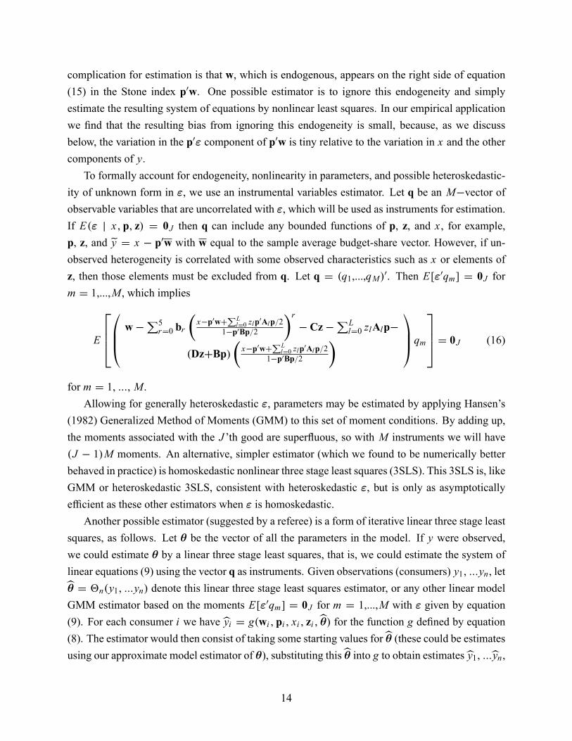
complication for estimation is that w, which is endogenous, appears on the right side of equation(15) in the Stone index p0w. One possible estimator is to ignore this endogeneity and simplyestimate the resulting system of equations by nonlinear least squares. In our empirical applicationwe �nd that the resulting bias from ignoring this endogeneity is small, because, as we discussbelow, the variation in the p0" component of p0w is tiny relative to the variation in x and the othercomponents of y.To formally account for endogeneity, nonlinearity in parameters, and possible heteroskedastic-

ity of unknown form in ", we use an instrumental variables estimator. Let q be an M�vector ofobservable variables that are uncorrelated with ", which will be used as instruments for estimation.If E." j x;p; z/ D 0J then q can include any bounded functions of p, z, and x , for example,p, z, and ey D x � p0w with w equal to the sample average budget-share vector. However, if un-observed heterogeneity is correlated with some observed characteristics such as x or elements ofz, then those elements must be excluded from q. Let q D .q1,...,qM/0. Then E["0qm] D 0J form D 1,...,M , which implies

E

26640BB@ w�

P5rD0 br

�x�p0wC

PLlD0 zlp0Alp=2

1�p0Bp=2

�r� Cz�

PLlD0 zlAlp�

.DzCBp/�x�p0wC

PLlD0 zlp0Alp=2

1�p0Bp=2

�1CCA qm

3775 D 0J (16)

for m D 1; :::;M .Allowing for generally heteroskedastic ", parameters may be estimated by applying Hansen's

(1982) Generalized Method of Moments (GMM) to this set of moment conditions. By adding up,the moments associated with the J 'th good are super�uous, so with M instruments we will have.J � 1/M moments. An alternative, simpler estimator (which we found to be numerically betterbehaved in practice) is homoskedastic nonlinear three stage least squares (3SLS). This 3SLS is, likeGMM or heteroskedastic 3SLS, consistent with heteroskedastic ", but is only as asymptoticallyef�cient as these other estimators when " is homoskedastic.Another possible estimator (suggested by a referee) is a form of iterative linear three stage least

squares, as follows. Let � be the vector of all the parameters in the model. If y were observed,we could estimate � by a linear three stage least squares, that is, we could estimate the system oflinear equations (9) using the vector q as instruments. Given observations (consumers) y1; :::yn , letb� D 2n.y1; :::yn/ denote this linear three stage least squares estimator, or any other linear modelGMM estimator based on the moments E["0qm] D 0J for m D 1,...,M with " given by equation(9). For each consumer i we have byi D g.wi ;pi ; xi ; zi ;b�/ for the function g de�ned by equation(8). The estimator would then consist of taking some starting values forb� (these could be estimatesusing our approximate model estimator of �), substituting thisb� into g to obtain estimatesby1; :::byn ,

14

do linear three stage least squares or linear model GMM using these by's as data to obtain a newvalue of � given by bb� D 2n.by1; :::byn/, and repeat this process using bb� in place b�, iterating toconvergence. This estimator could be easily implemented in a statistical package like Stata thatdoes linear three stage least squares or linear GMM regression. Note that imposing symmetryrestrictions requires imposing cross equation equality restrictions on the estimated coef�cients ineach iteration.Formally, let the �xed pointbb� D 2n h.g.w1;p1; x1; z1;bb�/; :::g.wn;pn; xn; zn;bb�//i de�ne the

estimatorbb�. This is a special case of the generic class of �xed point based estimators consideredby Dominitz and Sherman (2005), who provide associated consistency and limiting distributiontheory assuming that the mapping that de�nes the estimator bb� is a contraction mapping. If theiterations had been linear least squares seemingly unrelated regressions instead of linear threestage least squares regressions, then this estimator would also be an example of the iterated linearleast squares estimator for conditionally linear systems proposed by Blundell and Robin (1999).Blundell and Robin apply the estimator to a demand system context similar to ours, and providean extension to endogenous regressors, but their extension requires a control function form ofendogeneity that our model does not satisfy. We do not provide formal asymptotic theory for bb�in our model, but we found that this estimator performed very well in practice, yielding estimatesthat are numerically quite close to those of our full nonlinear three stage least squares estimator.The equality restrictions required for demand system rationality are easily imposed in our con-

text. Adding up and homogeneity constraints on the parameter vectors and matrices hold by omit-ting the J 'th good and imposing the linear restrictions that 1JAl D 1JB D 0. Slutsky symmetry issatis�ed if and only if Al for l D 0, ..., L and B are all symmetric matrices. All of these parametricrestrictions may be imposed as a set of linear constraints in 3SLS or GMM.Writing this system linearly as equation (9) suggests that good instruments q should be highly

correlated with p, z, zy, py, pz1, ...,pzL and yr . We assume E." j p; x; z/ D 0J and take q to bep, z, zy, py, pz1, ...,pzL , and yr for r D 0; :::; 5 with y de�ned as

y Dx � p0w�

PLlD0 zlp0Alp=2

1C p0Bp=2

where w is the average budget shares across consumers in our sample, and Al and B are theestimated values of Al and B based on linear least squares estimation of the approximate EASImodel. Note that use ofw and inconsistency of the estimates ofAl and B (due to their coming fromthe approximate model) in the construction of y only affects the quality of the instruments q andhence the ef�ciency of the 3SLS or GMM estimation, but does not cause inconsistency, becausey remains uncorrelated with " given any choice of values of the parameters w, Al and B in the

15

construction of y. When symmetry of Al and B is not imposed, this set of moments E."0qm/ D 0Jfor m D 1; :::;M exactly identi�es the EASI model parameters. Imposing symmetry reduces thenumber of distinct parameters, yielding overidenti�cation.Since we have assumed E." j p; x; z/ D 0J , we could interpret

P5rD0 br yr C Cz C Dzy as

a sieve approximation to a general unknown J�vector of smooth functions n.y; z/, with a span-ning basis consisting of functions of the form ysztk for integers s; t . Ai and Chen (2003) provideassociated rates of convergence, optimal instrument construction, and limiting distribution theoryfor general semiparametric sieve GMM estimators of this form. Such estimators can attain thesemiparametric ef�ciency bound for the remaining parameters, in this case Al and B.The parametric 3SLS or GMM estimators can be readily modi�ed to deal with possible mea-

surement error or endogeneity in some regressors, by suitably modifying the set of instruments q.For example, if simultaneity with supply is a concern (which is more likely to matter signi�cantlyin an aggregate demand context than in our empirical application), then we could replace p with peverywhere p appears in the construction of the instuments q, where p are the �ts from regressingp on supply side instruments.In many data sets, such as the UK Family Expenditure Survey, consumption is measured over a

very short time span and so is subject to considerable infrequency-based measurement error. In ourempirical application we use Canadian data where consumption is measured over an entire year,which implies less infrequency-based error, but may suffer from recall-based error. One mightdeal with this problem in part by including functions of income in place of functions of nominaltotal expenditures in our list of instruments. However, using an instrument like income, whichhas a large amount of over-time variation that is smoothed out in consumption decisions, mayentail considerable ef�ciency loss. One might alternatively use measures of household wealth asinstruments for total expenditure, but unfortunately, most public-use data sets (including ours) donot have both wealth and consumption data. It should also be noted that measurement errors intotal expenditures would affect not only our total expenditures regressor, but also the constructionof our dependent variables, the budget shares. Estimators such as Lewbel (1996) could potentiallybe used to deal with the latter problem.Similarly, if unobserved preference heterogeneity " is correlated with some observed taste

shifters (i.e., elements of z), then those may be excluded from the instrument list and replacedby, e.g, nonlinear functions of x and of the remaining elements of z. However, in these casesone would need to take care in interpreting the resulting model residuals b", because they willthen contain both unobserved preference heterogeneity and measurement error. With panel dataone might separate these two effects by modeling the unobserved preference heterogeneity usingstandard random or �xed effects methods. The exact model estimators remain consistent regardlessof heteroskedasticity in ", so for example the estimates are consistent if " D N.x; z/"� where "�

16

are preference parameters that are independent of p; x; z, and features of the functionN.x; z/ couldbe estimated based on the estimated conditional variance of residualsb", conditioning on x; z.The above described estimators do not impose the inequality (concavity and monotonicity) con-

straints implied by regularity of the cost function, or equivalently by utility maximization (globalregularity is discussed in the Appendix). In addition to these usual utility derived inequality con-straints, interpreting " as preference heterogeneity parameters requires " to be independent of p,and having the support of " independent of prices imposes additional inequality constraints (seethe Appendix for details). If the model is correctly speci�ed then imposing these inequality con-straints on parameter estimates will not be binding asymptotically, and so failing to impose themwill not result in a loss of asymptotic ef�ciency, as long as the true parameter values do not lie onthe boundary of the feasible region implied by the inequality constraints. Based on this, a commonpractice in empirical demand analysis, which we will follow in our application, is to estimate themodel without imposing inequality constraints, and then check that they are satistifed for a rea-sonable range of p, x , and z values. In particular, the inequalities associated with utility functionregularity are readily veri�ed using elasticity calculations, e.g., the estimated Slutsky matrix canbe checked for negative semide�niteness.

3.2 Data and Model Tests

We �rst estimate the approximate EASI model, equation (11) withey given by equation (10), usingSUR. We then estimate the exact EASI model given by (15) by nonlinear 3SLS with instrumentsand starting values as described in the previous section. We use 3SLS because we found the GMMweighting matrix estimates to be numerically unstable. Also, 3SLS is asymptotically ef�cientunder the assumption of independently distributed ", and our 3SLS estimator remains consistent(though inef�cient) if " is not homoskedastic.The data used in this paper come from the following public use sources: (1) the Family Ex-

penditure Surveys 1969, 1974, 1978, 1982, 1984, 1986, 1990, 1992 and 1996; (2) the Surveysof Household Spending 1997, 1998 and 1999; and (3) Browning and Thomas (1999), with up-dates and extensions to rental prices from Pendakur (2002). Price and expenditure data are usedfrom 12 years in 4 regions (Atlantic, Ontario, Prairies and British Columbia) yielding 48 distinctprice vectors. Prices are normalised so that the price vector facing residents of Ontario in 1986 is.1; :::; 1/, that is, these observations de�ne the base price vector p D 0J . Since the model containsa high-order polynomial in y, we subtract the median value of x � p0w from y. Translating y bya constant is absorbed by changes in the A0, br and C coef�cients leaving the �t unchanged, andshifting y to near zero reduces numerical problems associated with data matrix conditioning bygiving the br coef�cients comparable magnitudes.

17

The empirical analysis uses annual expenditure in J D 9 expenditure categories: food-in,food-out, rent, clothing, household operation, household furnishing & equipment, transportationoperation, recreation and personal care. Personal care is the left-out equation, yielding eight expen-diture share equations to be estimated. These expenditure categories, which exclude large durables,account for about 85% of the current consumption of the households in the sample.Our sample for estimation consists of 4847 observations of rental-tenure single-member house-

holds who had positive expenditures on rent, recreation and transportation. We use only personsaged 25 to 64 living in cities with at least 30,000 residents. We use residents of English Canadaonly (so Quebec is excluded). Single-member households are used to avoid issues associated withbargaining or other complications that may be associated with the behavior of collective house-holds. City residents are used to minimise the effects of possible home and farm production. Table1 gives summary statistics for our estimation sample.We include L D 5 observable demographic characteristics in our model: (1) the person's age

minus 40; (2) the sex dummy equal to 1 for men; (3) a car-nonowner dummy equal to 1 if realgasoline expenditures (at 1986 gasoline prices) are less than $50; (4) a social assistance dummyequal to 1 if government transfers are greater than 10% of gross income; and (5) a time variableequal to the calendar year minus 1986 (that is, equal to zero in 1986).We include the time variable in the model to account for possible slow changes over time in

tastes, quality, and composition of composite goods. Time trends are also commonly includedin demand systems to account for some types of habit formation (see, e.g., Pollak and Wales1992). The time trend may also help to compensate for average growth in, and hence possiblenonstationarity of, real total expenditures over time, noting that our dependent variables, budgetshares, are bounded. See, e.g., Lewbel and Ng (2005) for a detailed analysis of the effects ofcovariate nonstationarity in budget-share demand-system models. However, our data consist ofrepeated cross sections at the household level, so the scope for possible dependence of errorsacross observations due to total expenditure growth is limited.These variables are all zero for a 40 year old car-owning female in 1986 who did not receive

much government transfer income. We use a limited set of characteristics like this because eachadditional element of z increases the number of additional parameters to estimate in our modelby 52 (80 additional parameters minus 28 additional symmetry restrictions). One could introduceadditional demographics at a lower cost in degrees of freedom by including a large set of char-acteristics in the m function (the C and D parameter matrices) and a smaller set interacted withprices (the Al matrices). Restrictiveness of the observed heterogeneity speci�cation is also partlymitigated by the relative demographic homogeneity of the sample, and by the role of " whichembodies unobserved preference heterogeneity.When symmetry is not imposed on Al and B, then given the instruments speci�ed above, the

18

model is exactly identi�ed. Denoting the number of terms in each br (6 in our baseline model) asR, the symmetry-unrestricted model has [R C L C L C .J � 1/.L C 1/C .J � 1/] .J�1/ D 576parameters for br ; C, D, Al , and B (72 coef�cients in each of 8 equations). When symmetry isimposed on Al and B, the model has .L C 2/ .J � 1/ .J � 2/ =2 D 196 restrictions, which areoveridentifying restrictions for testing exogeneity and are also symmetry restrictions. Since eachestimated model has hundreds of parameters, we do not present all the individual coef�cientsestimates (they are available from the authors on request). We instead provide many summariesand analyses of the results. Even with parameters all set to zero as starting values, we still obtainedconvergence of the nonlinear 3SLS exact model estimator in only three iterations, due to the nearlinearity of the EASI model.Table 2 gives Wald- and J-tests for various hypotheses concerning the model. Since our sample

size is large (8 equations times 4847 observations per equation) we use a 1% critical value for alltests. Consider price effects �rst. The Wald test of symmetry in the asymmetric model is mar-ginally insigni�cant with a p-value of 1.4%, and symmetry is not rejected for either the level ofprices (Al D A0l for all l) or for prices interacted with implicit utility y (B D B

0). This lack of sym-metry rejection is not due to the irrelevance of price effects. In particular, the direct price effectsgiven by the A0 matrix are strongly signi�cant, as are many of the interactions between prices anddemographics in the Al matrices. The interaction of prices with income are less signi�cant, andwe cannot reject the hypothesis that the py interaction given by the B matrix is excludable.Turning to expenditure effects, we �rst check for adequacy of our �fth order polynomial in y

by adding either a y�1 or y6 term to the model. The reciprocal of y is excludable with a p-valueof 4.9%. The 6th order term in y is marginally signi�cant, but these tests covary, and the joint testof exclusion of both y�1 and y6 is not signi�cant, with a p�value of 2.9%. Taken together theabove results suggest that symmetry may not be violated and that a 5th order polynomial in y maybe suf�cient, so we present further results for a symmetry-restricted model with r D 0; 1; ::; 5.The lower panel of Table 2 shows that one cannot further reduce the level of the polynomial in y

by dropping y5. Turning to evidence of complicated Engel curve shapes, we test for whether or noteach of the 8 budget share equations can be reduced to a quadratic. The tests suggest that 4 of the 8budget shares are statistically signi�cantly nonquadratic: food-at-home, rent, household operation,and recreation. These departures from quadratic Engel curves suggest that allowing for complexEngel curves is a useful attribute of our methodology. Later we examine our estimated Engelcurve shapes in more detail, considering whether the departures from quadratic are economicallyimportant in addition to statistically signi�cant.Next consider some model summary statistics. The symmetry-restricted model is overiden-

ti�ed, so we can construct overidenti�cation tests of instrument validity. The 196 symmetry-restrictions result in our model having 196 more moments than parameters, and we pass the re-

19

sulting overidenti�cation based test of validity of the included moments with a p-value of 2.1%.However, if we include additional instruments based on y�1 and y6, we obtain 16 additional mo-ments (two more instruments times eight budget share equations), and the resulting J-test of overi-dentifying restrictions becomes marginally signi�cant.Let e denote the sample residuals vector, which is also our estimate of " for each household.

The R2 values for the 8 equations (in the order given in Table 2) are: 0.49, 0.31, 0.65, 0.30, 0.19,0.43, 0.57, and 0.31, respectively. The model is not estimated by ordinary least squares, so theseR20s should only be interpreted as summary measures regarding the size of e relative to budgetshares. These numbers show that much, even most, of the variation in budget shares is due tounobserved heterogeneity. Our approach formally includes " as random utility parameters, sothe relatively large variation in e yields large effects in our welfare calculation estimates, as wedemonstrate below.Table 3 gives information on the sources of variation in y. Since both total expenditures and

prices may contain time trends, we detrended all the variables in this table by regressing them ondummies for each time period, and report correlations of the resulting residuals from these regres-sions. The upper block of Table 3 gives standard deviations and pairwise correlations betweenthree variables. The �rst is y itself, detrended. The second, denoted y.p0.w � e// is identical toy except that it removes p0e, from the p0w component of y given in equation (8). The third isthe instrument y, which is identical to y, except that it has p0w, where w is the sample-averagebudget-share vector, in the numerator instead of p0w. These three variables have almost identicalvariances and correlations over 0.998 even after detrending. This shows that the instrument y ishighly relevant, and that, while our estimator controls for endogeneity in y, it may not be numer-ically important to do so in practice, since removing the source of endogeneity from y leaves itvirtually unchanged.Further examining the components of y, the second block of Table 3 shows correlations be-

tween y and two measures of log of stone-de�ated expenditures, x � p0w andey D x � p0w. Evenafter detrending these variables are also highly correlated with each other, which explains whythe approximate EASI model estimates are close to the exact model estimates, even though theapproximate EASI does not include the af�ne transformation of x � p0w that de�nes y, and ourapproximate EASI estimates do not control for endogeneity.The third block of Table 3 considers the magnitude of p0e in more detail. Here, we see that the

standard deviation of p0e is about one-twentieth as large as that of y and of the log of stone-de�atedexpenditures, x�p0w, and that p0e is only weakly correlated with these real expenditure measures.This again shows that the endogenous component of y orey is small. It also shows that if the errorsin our model were treated as measurement errors in budget shares (or more generally, as errors thatare non-behavioral or otherwise not part of the model), then our parameter estimates (including our

20

�nding of signi�cantly nonquadratic Engel curves) would be almost unchanged. However, treatingthe errors as measurement errors rather than preference heterogeneity parameters substantially af-fects consumer surplus and social welfare calculations, as we show later in the section on consumersurplus estimates. Formally excluding p0" from y requires iterative estimation, following the spiritof the iterative nonparametric approach proposed in Pendakur and Sperlich (2005). We discuss theresults of such estimation at the end of section 3.5.The last block of Table 3 gives the standard deviation and correlations of

PLlD0 zlp0Alp=2

(denoted p'Ap in the Table) and p0Bp=2, which are the components of the difference between yand x�p0w. These components have less than one-tenth the standard deviation of p0e and less thana hundredth the standard deviation of y. As a result, they only drive a tiny fraction of the variationin y, which again shows why the approximation that ignores these components is quite good.

3.3 Estimated Engel Curves

The easiest way to summarize the income related parameter estimates is to examine the resultingexpenditure share equations as functions of x for particular values of p, z, and ". At p D 0J ,y equals log nominal expenditure x , so at these base prices we obtain Marshallian Engel curvesw D

P5rD0 br xrCCzCDzxC". Figures 1-8 show these estimated Engel curves from our model for

a 40 year old car-owning female in 1986 who did not receive much government transfer income,and having " D 0. For her, w D

P5rD0 br xr . The base period Engel curves for households with

different values of unobserved heterogeneity are identical except for being vertically shifted by". These base period Engel curves are also informative about the shape of Engel curves in otherprice regimes, since at other price vectors, Engel curves expressed in terms of our real expendituresmeasure y differ from the above only by the addition of the linear function

PLlD0AlzlpC Bpy.

In Figures 1 to 8, each �gure presents the estimated Engel curve for four models: thick blacklines indicate 3SLS estimates of the symmetry-restricted exact model; thick grey lines indicate3SLS estimates of the symmetry-restricted quadratic (having a second instead of �fth order poly-nomial in y) exact model; dotted thick black lines indicate approximate SUR estimates of themodel; and thin black lines indicate exact 3SLS estimates of the asymmetric model (italics denoteshorthand). Estimates are computed at each percentile of log expenditures in the data, and esti-mated 90% con�dence intervals (computed via the delta method) are displayed with small crossesfor the exact 3SLS symmetry-restricted model at each �fth percentile of the expenditure distribu-tion.As noted earlier, our quadratic speci�cation is very similar to Quadratic Almost Ideal (QAI)

related models estimated by Blundell, Pashardes, and Weber (1993) and Banks, Blundell and Lew-bel (1997). The quadratic EASI differs from these QAI models in that it has a different de�ator for

21

total expenditures, and it does not require the coef�cient of squared y to either depend on prices oron the lower order expenditure coef�cients to stay consistent with utility maximization. Our spec-i�cation also allows for more general demographic effects than is typical in applied QAI models,which usually only have terms analogous to C, but not Al or D.Figures 1 and 2 show Engel curves for food-in (food consumed at home) and food-out. Both

these Engel curves are almost linear. Both the approximate and quadratic symmetry-restrictedmodels lie within the 90% pointwise con�dence intervals of the exact model. However, in thefood-out equation, the asymmetric model estimates are above the con�dence intervals in the upperpart of the expenditure distribution. The food-in budget share equation is statistically signi�cantlynon-quadratic (see Table 2), though the empirical size of the departure is small.Figure 3 shows the Engel curve for rent. Throughout most of the expenditure distribution, the

quadratic estimates lie outside the con�dence intervals of the exact estimates. In the exact esti-mates, the curvature of the Engel curve is near zero in the bottom decile, strongly negative in thenext two deciles, and near zero until it becomes positive in the top decile. This kind of complex-ity cannot be captured in a quadratic model but is readily accomodated in the EASI framework.Further, the magnitude of the quadratic departure from the exact model can be large. At the �fthpercentile, the quadratic model overestimates the rent budget share by almost 5 percentage points.At the bottom quintile cutoff, the quadratic model underestimates the rent budget share by about 2percentage points.For the rent equation, the approximate model performs very well, lying essentially on top of

the exact estimates throughout the distribution of expenditures. As in the food-out equation, theasymmetric model performs relatively poorly (though not as poorly as the quadratic model).Figures 4, 5, 6 and 7 give the household operation, household furnishing & equipment, clothing

and transportation operation Engel curves. All four sets of estimates lie within the 90% con�denceintervals of the exact model estimates. However, as shown in Table 2, the household operationequation shows evidence of being statistically signi�cantly nonquadratic. The departure fromquadratic can be seen in Figure 4, where the exact model estimate looks more like two nearlylinear segments joined by a curved segment in the middle instead of a true quadratic function.Figure 8 gives the recreation Engel curve. As in Figures 4-7, all four sets of estimates lie within

the pointwise con�dence intervals of the exact model estimates. However, as in the rent equation,the quadratic model is statistically rejected (see Table 2), and the Engel curve looks nonquadratic,particularly in the bottom decile, where the exact model estimate of the recreation Engel curve�attens out, while the quadratic estimate has a strong negative slope.We now address the question of whether the complexity we observe in our estimated Engel

curves is an artifact of our sample or of our choice of modeled expenditure categories. In particu-lar, much of the nonquadratic behavior we observe is in the tails of the x distribution, where data

22

are relatively sparse. In addition, many researchers of consumer demand exclude shelter expen-ditures (ie., rent) on the grounds that such expenditures cannot be adjusted quickly in the face ofbudget and price changes. A possible concern is whether the nonlinearity we observe in the rentshare arti�cially induces nonlinearity in other estimated budget share functions. We conduct threerobustness exercises aimed at these issues. First, we estimated our EASI model using an extendedsample of 18,600 households, which includes multiple-member households and households resid-ing in Quebec. For this model, we included 4 additional demographic variables: the log of thenumber of household members, and dummies indicating single-parent households, childless cou-ple households and households residing in Quebec. Second, we estimated our EASI model on the8846 households in our extended sample that did not have transfer income exceeding 10% of grossincome and who did own a car (called the `nopoor' extended sample). Third, we estimated ourEASI model on a subset of expenditure categories which excludes rent. For this model, we usedhouseholds of all tenures, not just rental-tenure households, and used only those that did not havetransfer income exceeding 10% of gross income and that did own a car. This yielded 32,399 obser-vations available for an estimation sample (called the `norent nopoor' extended sample). For thenorent nopoor extended sample, we include the number of rooms in the dwelling and its square asadditional demographic characteristics. Detailed results for these models are available on requestfrom the authors.Figures 9 and 10 show the estimated rent and recreation Engel curves for various samples for

the reference type de�ned above facing the base price vector, plus con�dence intervals (shownwith x's) for the Engel curves of the extended sample. Engel curves are evaluated at each �fthpercentile of the single-person household real-expenditure distribution for the sample. Con�denceintervals for other samples are similar in size, and are suppressed to reduce clutter. Examinationof Figure 9 shows that the non-quadratic curvature we noted in Figure 3 for the rent Engel curveremains evident in the much larger extended sample (thin black line). Of course, the extendednopoor sample (dotted line) is uninformative at the bottom of the distribution because excludesthe poor, but it does reveal some departure from the quadratic model at the high end: at the 97thpercentile of the nopoor distribution, then EASI Engel curve is 2 percentage points (and statisticallysigni�cantly) higher than the quadratic model would indicate.Figure 10 gives Engel curves for the baseline sample, the extended sample, the extended nopoor

sample and the extended nopoor norent sample. The �gure shows that the curvature in the recre-ation Engel curve observed at the bottom end of the expenditure distribution in Figure 8 may haveoverstated the change in curvature for poor households. In particular, the extended sample (thinblack line) does not reveal much nonquadratic curvature at the bottom of the distribution. Unsur-prisingly, since the curvature was seen mainly at the bottom, the extended nopoor sample (dottedline) does not pick it up either. Also, in the larger sample at the upper end of the expenditure distri-

23

bution, the three bunched recreation Engel curves lie within each others' 90% con�dence intervals.Turning to the extended nopoor norent sample (thick grey line), wherein the rent equation is notmodeled and a much larger number of observations is used, apart from a slight upturn at the verybottom of the distribution, we see little evidence of important non-quadratic curvature.There are two important lessons that we draw from these �gures. First, the SUR estimates

of the approximate model do quite a good job of approximating the Engel curve estimates of theexact model, even when the underlying Engel curves are quite complex. Second, while the demandfunctions of some goods are close to linear or quadratic in log total expenditures, other goods suchas rent and recreation are not quadratic. This implies a demand system rank (see Gorman 1981and Lewbel 1991) that is higher than three. Most past empirical studies have found rank to equalthree, though Lewbel (2003) �nds some empirical evidence for rank four. Figures 1 to 10 suggestthat the reason why previous studies failed to �nd ranks higher than three is because most of thedepartures from quadratic are either somewhat subtle, as in the household operation equation, orare concentrated in the tails of the expenditure distribution as in the rent equation. Either way, theprecision gained by detailed model speci�cation and large sample sizes is needed to con�rm thedeparture from quadratic Engel curves.

3.4 Estimated Price Effects

Prices in our model vary only by region and year, so despite having thousands of observations weonly have 48 different price regimes. However these data still contain a very substantial amount ofrelative price variation, both because our sample is spread out over 28 years, and because Canadahas historically had considerable regional price variation in some goods and services. As a result,we are able to obtain a reasonable amount of precision in many of our price effect estimates.In our framework, price effects are most easily evaluated by looking at compensated budget-

share semi-elasticities, compensated (good-speci�c) expenditure elasticities, or compensated quan-tity derivatives (aka, Slutsky terms). As shown by equation (12), compensated budget-share semi-elasticities with respect to prices are given by the matrix 7 �

PLlD0Alzl C By, and so are af�ne

in z and y. Compensated (good-speci�c) expenditure elasticities with respect to prices is closelyrelated, and is given byW�1 �7 C ww0� whereW D diag.w/. The normalised1 Slutsky matrix,S, is related to the compensated semi-elasticity matrix, 7 , by S D 7 Cww0�W. Table 4 assessesall 3 of these measures of price effects. Since y D x at the base price vector, and since x D 0at median expenditure, this matrix is equal to A0 at median expenditure for the reference type of

1The Slutsky matrix, S, is de�ned as the matrix of compensated quantity derivatives with respect to (unlogged)prices. The normalised Slutsky matrix;S, (see Pollak and Wales 1990) normalises the Slutsky matrix for prices andexpenditure: S D PSP=x , where P D diag.exp.p//. Concavity of cost is necessary and suf�cient for negativesemide�niteness of both the Slutsky matrix and the normalised Slutsky matrix.

24

person, a 40 year old car-owning female in 1986 who did not receive much government transfer in-come. Table 4 presents summary estimated price effects, with asymptotic standard errors in italics.The rightmost block of Table 4 gives compensated price semi-elasticities for a reference personwith median expenditure from the symmetry-restricted exact 3SLS estimates.Consider �rst the matrix of compensated budget-share semi-elasticities for the reference person

at median expenditure given by A0. Several of the own-price effects are large and statisticallysigni�cant. The own-price compensated semi-elasticity for the rent budget share is 0.063, whichimplies that a rent price increase of 10% would be associated with a budget share 0.63 percentagepoints higher when expenditure is raised to equate utility with that in the initial situation. Incontrast, if the recreation price rises by 10%, its budget share will be a little more than 1 percentagepoint lower when expenditure is raised to compensate for the loss in utility.Several cross-price effects are also large and statistically signi�cant, suggesting that substitu-

tion effects are important. For example, the clothing budget share compensated rent cross-pricesemi-elasticity is -0.066, implying that an increase in the price of rent is associated with a sig-ni�cant decrease in the budget share for clothing even after expenditure is raised to hold utilityconstant.For some readers, expenditure elasticities may be more easily interpreted than budget-share

semi-elasticities. In order to pin down these elasticities, we additionally need to specify the un-observed heterogeneity terms, which enter w (but don't enter 0). For the reference type at me-dian expenditures with " D 0J , we may calculate elasticities using A0 and the level of the bud-get share function at median expenditure. The own-price expenditure elasticities are given in thethird column of Table 4, with asymptotic standard errors computed via the delta method in italics.(The variance of these elasticities is driven by the variance of the own-price compensated semi-elasticities, 0, and so reported standard errors are very close to those standard errors de�ated bythe appropriate budget share.) Unsurprisingly, only those equations with statistically signi�cantown-price compensated budget-share semi-elasticities have statistically signi�cant compensatedexpenditure elasticities. In particular, compensated rent expenditures have an elasticity of 0:528and compensated transportation operation expenditure have an elasticity of 0:393. In contrast,compensated recreation expenditures are highly negatively elastic, with a marginally statisticallysigni�cant own-price expenditure elasticity of �1:191.Although some of the own-price elasticities and semi-elasticities in Table 4 are statistically

signi�cantly positive, this does not imply that concavity (negative semi-de�niteness) is violated.Concavity of cost is satis�ed if and only if S is negative semi-de�nite (see, e.g., Pollak and Wales1992). For the case where " D 0J , the Slutsky matrix for the reference type with median ex-penditure facing base prices is fully speci�ed by the matrix A0 and the value of the Engel curvefunctions at median expenditure. The values of the own-price Slutsky terms are reported in the

25

second column of Table 4, with asymptotic standard errors computed via the delta method in ital-ics. A glance down this column reveals that the own-price Slutsky terms are all negative, and mostare statistically signi�cant. In addition, the Slutsky matrix evaluated at median expenditure for thereference type facing base prices is negative semide�nite, implying that the cost function is weaklyconcave at this point in the data.The leftmost column of estimates in Table 4 contains the estimated own-price elements of B,

which show the magnitudes of the interaction between own-prices and with log total expenditures.These parameters allow us to assess whether or not compensated semi-elasticities are the same forrich and poor households. As noted in our discussion of Table 2, we cannot strongly reject thejoint hypothesis that the entire matrix B is zero, so these results must be interpreted with caution.However, the estimated coef�cient of the rent own-price compensated semi-elasticity on y is 0:088,and is by itself marginally statistically signi�cant. Consider the comparison between the rentown-price compensated semi-elasticity for a reference person at the 5th percentile of expenditure(x D �0:90) versus that for such a person at the 95th percentile of expenditure (x D 0:60). Asnoted above, its value at the median expenditure of x D 0 is �0:066. At the 5th percentile, itsvalue is �0:066 � 0:90 � 0:088 D �0:016, and is insigni�cantly different from zero. In contrast,at the 95th percentile, its value is �0:066C 0:60 � 0:088 D 0:115, and appears highly statisticallysigni�cant. The corresponding own-price rent Slutsky terms are �0:236 at the �fth percentile and�0:080 at the 95th percentile, and both are statistically signi�cantly negative. These results suggestthat poor households substitute much more than do rich households in the face of an increase inthe price of rent.We draw three main conclusions from the analysis of price effects. First, we are able to obtain

estimates of compensated elasticities, which given symmetry are second-order derivatives of thelog-cost function and capture substitution effects. Uncompensated elasticities can also be calcu-lated (see the Appendix for details). These elasticity estimates suggest that some price effects, andtherefore substitution effects, are large in magnitude. Our second conclusion is that the rationalityrestriction of concavity is not violated, at least for the reference type. Third, there is some evi-dence that substitution effects are different for rich and poor households, and speci�cally, that poorhouseholds substitute much more in the face of rental price increases than do rich households.

3.5 Consumer Surplus Estimates

We assess the economic signi�cance of our models with a cost-of-living experiment. In Canada,rent is not subject to sales taxes, which typically amount to 15% for goods such as food-out andclothing. Consider the cost-of-living index associated with subjecting rent to a 15% sales tax for

26

people facing the base price vector, so that p0 D 0J and p1 D [0 0 ln 0:15 0 0 0 0 0 0] :

C.p1; u; z; "/� C.p0; u; z; "/ D ln 0:15wrent C ln 0:152

LXlD0zlarent;rentl C brent;rent y

!=2

D ln 0:15wrent C ln 0:152

LXlD0zlarent;rentl C brent;rent x

!=2

where arent;rentl and brent;rent are the rent own-price elements of Al and B. We choose 0J asthe comparison price vector because at this price vector, y D x , and as a consequence only 1budget share and 6 parameters are needed to estimate the cost-of-living index. Here, unobservedheterogeneity enters only through the level effect on wrent . We can think of this cost of livingindex as being comprised of two effects: a �rst-order effect which is driven by expenditure sharesand which incorporates unobserved heterogeneity; and a second-order effect which captures sub-stitution effects. Traditional consumer demand analysis which ignores unobserved heterogeneitywould accomodate both �rst- and second-order effects, but would use bwrent , which contains no `er-ror term', rather than wrent which contains an unobserved preference heterogeneity component. Incontrast, traditional nonparametric approaches to the cost-of-living would use only the �rst-orderterm which accomodates unobserved heterogeneity, but would not incorporate the second-orderterm which captures substitution effects. Our model combines the advantages of both approaches.Figure 11 shows the estimated values of the cost-of-living index for each household facing

the base price vector in our baseline sample incorporating unobserved heterogeneity with emptycircles and shows estimated values for each household with unobserved heterogeneity set to zero(" D 0) using �lled circles. In addition, the second-order component capturing substitution effectsis shown with �lled squares. The reason that the �lled circles and �lled squares do not each lie ona single line is that variation in demographic characteristics z across households affect the surplusmeasures.The underlying Engel curve is visible in the estimates which zero out ", but is largely obscured

when this unobserved heterogeneity is taken into account. Failure to account for unobserved het-erogeneity leads to the erroneous impression that most of the variation across individuals in thecost-of-living impact of a large rent increase is related to expenditure, and only a little is relatedto other characteristics. The more re�ned picture is that most of the variation in the impact oncost-of-living is attributable to unobserved characteristics. Even in a model as rich as ours, withmany hundreds of parameters, most of the variation in demand is due to unobserved characteris-tics, and this is re�ected in the variation in cost of living responses. As noted earlier, our parameterestimates would be little changed if some or all of the errors were interpreted as ordinary model-ing error rather than preference heterogeneity. In this case, the cost of living impacts would lie

27

somewhere between the �lled and empty circles in Figure 11.Figure 11 also shows the need for highly �exible Engel curves. The �rst-order term in the

consumer surplus calculation is driven by the Engel curve, and as Figure 3 shows, even a quadraticprovides a poor approximation to the rent expenditure share equation, so demand systems that onlyallow for linear or quadratic Engel curves can make substantial errors in policy analyses. Theseerrors would be magni�ed in a policy experiment that more directly affected the distribution oftotal expenditures, such as a change in the progressivity of income taxes.The second-order terms above capture substitution effects across expenditure share equations.

These effects are not large in this experiment, but they do have a pronounced pattern, as shownby the �lled squares in Figure 11. If consumers substitute greatly in the face of price increases,then the second-order terms will be large and negative; if they substitute little, the the second-order terms will be large and positive. Since the poor substitute more than the rich, second-ordereffects are positively related to expenditure, so ignoring them would result in underestimatingthe cost-of-living impact for rich households and over-estimating the impact for poor households.The magnitude of the second-order term is about -0.1 percentage points for households at the5th percentile (on a total impact of about 6 percentage points), and its magnitude is about +0.1percentage points for households at the 95th percentile (on a total impact of about 4 percentagepoints).As noted above, the treatment of " as unobserved preference heterogeneity parameters rather

than as measurement error affects consumer surplus measures greatly. However, it turns out not toaffect estimated parameters of the model very much. We re-estimated the EASI model assuming" is measurement error via an iterative procedure. First, we estimate the exact EASI model, andthen compute y.p0.w � e// as in Table 2, which is identical to y except that it has p0e subtractedfrom the numerator in the de�nition of y given in equation (8). Then, we estimate the approximateEASI model using y.p0.w� e// asey, re-compute y.p0.w� e//, re-estimate the approximate EASImodel, and iterate to convergence (4 iterations). The resulting estimated parameter vector is veryclose to the exact EASI estimated parameter vector. The maximum absolute distance betweenparameters of 0.1 standard error (using the exact EASI estimated standard errors), and the averageabsolute distance is 0.005 standard error. In terms of an economic measure of difference, using the`measurement error' version of the model to assess cost-of-living impacts as in Figure 11 yieldsestimates visually identical to the �lled black circles in the Figure. The maximum absolute distancebetween the �lled black circles in the Figure and the `measurement error' version of cost-of-livingestimates is 0.01 percentage points, which is negligible in comparison to the estimated values ofaround 5 percentage points.

28

4 Conclusions

We invent implicit Marshallian demand systems. These are the compensated budget share func-tions (Hicks demands) associated with cost functions having the property that utility can be rep-resented by a simple function of observables, including budget shares themselves. We show thatsimple implicit Marshallian demand systems allow us to solve many problems facing consumer de-mand analysis, including the incorporation of unobserved preference heterogeneity and allowingfor �exibility in Engel curves.We provide the Exact Af�ne Stone Index (EASI) implicit Marshallian demand system, in which

utility is ordinally equivalent to an af�ne function of the log of expenditure de�ated by the StoneIndex. This EASI demand system is as �exible in price responses, as close to linear in parameters,and as easy to estimate as the Almost Ideal Demand (AID) system. But, in contrast to the AIDsystem, the EASI demand system also allows for �exible interactions between prices and expendi-tures, permits almost any functional form for Engel curves, and allows error terms in the model tocorrespond to unobserved preference heterogeneity random utility parameters. Demand functionsmay be estimated by 3SLS or GMM, and, like the AID system, an approximate model can beestimated by linear regression. We estimate the model, and �nd some signi�cant departures fromlinear and quadratic demands. We also �nd that allowing errors to equal unobserved preferenceheterogeneity has little effect on model parameter estimates, but substantially affects social welfarecalculations such as the cost of living impacts of price changes.

References[1] Ai, Chunrong and Xiaohong Chen (2003), "Ef�cient Estimation of Models with Conditional

Moment Restrictions Containing Unknown Functions," Econometrica, 71, 1795-1944.

[2] Banks, James, Richard Blundell, and Arthur Lewbel (1997), "Quadratic Engel curves andConsumer Demand," Review of Economics and Statistics, 79, 527�539.

[3] Beckert, Walter and Richard Blundell (2004), "Invertibility of Nonparametric Stochastic De-mand Functions," Birkbeck Working Papers in Economics and Finance No. 406.

[4] Blackorby, Charles, and David Donaldson (1980), "TheoreticalTreatment of Indices of Ab-solute Inequality," International Economic Review, 21, 107-136.

[5] Blackorby, Charles, and David Donaldson (1993), "Adult-Equivalence Scales and the Eco-nomic Implementation of Interpersonal Comparisons ofWell-Being," Social Choice andWel-fare, 10, 335-61.

[6] Blundell, Richard, Xiaohong Chen and Dennis Kristensen (2007), "Nonparametric IV Esti-mation of Shape-Invariant Engel curves," Econometrica, 75, 1613�1669.

29

[7] Blundell, Richard, Alan Duncan and Krishna Pendakur (1998), "Semiparametric Estimationof Consumer Demand", Journal of Applied Econometrics 13, 435-461.

[8] Blundell, Richard and Arthur Lewbel (1991), "The Information Content of EquivalenceScales." Journal of Econometrics 50, 49-68.

[9] Blundell, Richard, Panos Pashardes, and Guglielmo Weber (1993), �What do we learn aboutConsumer Demand Patterns from Micro Data?�, American Economic Review, vol. 83, 570-597.

[10] Blundell, Richard and Robin, JeanMarc, (1999), "Estimation in Large and Disaggregated De-mand Systems: An Estimator for Conditionally Linear Systems," Journal of Applied Econo-metrics, 14, 209-232.

[11] Brown, Donald J. and Rosa L. Matzkin, (1998), "Estimation of Nonparametric Functions inSimultaneous Equations Models, with an Application to Consumer Demand," Cowles Foun-dation Discussion Papers 1175, Cowles Foundation, Yale University.

[12] Brown, Bryan W. and Mary Beth Walker (1989), �The Random Utility Hypothesis and Infer-ence in Demand Systems� Econometrica 57, 815-829

[13] Browning, Martin, Pierre-Andre Chiappori and Arthur Lewbel, (2004) "Estimating Con-sumption Economies of Scale, Adult Equivalence Scales, and Household Bargaining Power,"Boston College Working Papers in Economics 588.

[14] Browning, Martin and Irena Thomas, (1999) "Prices for the FAMEX," unpublished workingpaper, Department of Economics, McMaster University.

[15] Browning, Martin, (2001), Modelling Commodity Demands and Labour Supply with M-Demands, unpublished working paper, Institute of Economics, University of Copenhagen.

[16] Deaton, Angus S., and John Muellbauer (1980), �An Almost Ideal Demand System,� Amer-ican Economic Review, vol. 70, 312-326.

[17] Diewert, Walter Erwin. and Terrence J. Wales (1987), "Flexible Functional Forms and GlobalCurvature Restrictions," Econometrica, 55. 43-68.

[18] Dominitz, Jeff and Robert P. Sherman (2005), "Some Convergence Theory for Iterative Esti-mation Procedures with an Application to Semiparametric Estimation," Econometric Theory,21, 838-863.

[19] Gorman, William M. "Tricks with utility functions", in Artis, M. and A. R. Nobay (eds.),Essays in Economic Analysis, Cambridge University Press (1976).

[20] Gorman, William M. (1981), "Some Engel Curves," in Essays in the Theory and Measure-ment of Consumer Behaviour in Honor of Sir Richard Stone, ed. by Angus Deaton, Cam-bridge: Cambridge University Press.

[21] Hansen, Lars, (1982), �Large Sample Properties of Generalized Method of Moments Estima-tors,� Econometrica, 50, 1029-1054.

30

[22] Hildenbrand, Werner, (1994), Market Demand, Princeton University Press.

[23] Lewbel, Arthur (1989). "Household Equivalence Scales and Welfare Comparisons," Journalof Public Economics, 39, 377-91.

[24] Lewbel, Arthur (1991), �The Rank of Demand Systems: Theory and Nonparametric Estima-tion,� Econometrica, 59, 711-730.

[25] Lewbel, Arthur (1996), �Demand Estimation with Expenditure Measurement Errors on theLeft and Right Hand Side," The Review of Economics and Statistics, 78(4), 718-725.

[26] Lewbel, Arthur (2001), "Demand Systems with and without Errors," American EconomicReview, 91, 611-618

[27] Lewbel, Arthur (2003), "A Rational Rank Four Demand System," Journal of Applied Econo-metrics, 18, 127-135.

[28] Lewbel, Arthur and Serena Ng, (2005), "Demand Systems with Nonstationary Prices," TheReview of Economics and Statistics, 87(3), 479-494.

[29] Matzkin, Rosa L. (2005), �Heterogeneous Choice,� for Advances in Economics and Econo-metrics, edited by Richard Blundell, Whitney Newey, and Torsten Persson, CambridgeUniversity Press; presented at the Invited Symposium on Modeling Heterogeneity, WorldCongress of the Econometric Society, London, U.K.

[30] McFadden, Daniel. and Marcel K. Richter (1990), �Stochastic Rationality and Revealed Sto-chastic Preference,� in J. Chipman, D. McFadden, M. K. Richter (eds) Preferences, Uncer-tainty, and Optimality, Essays in Honor of Leo Hurwicz, 161-186, Westview Press: Boulder,CO.

[31] Pendakur, Krishna (1999) "Estimates and Tests of Base-Independent Equivalence Scales,"Journal of Econometrics, 88, 1-40.

[32] Pendakur, Krishna (2002) "Taking Prices Seriously in the Measurement of Inequality," Jour-nal of Public Economics, 86, 47-69.

[33] Pendakur, Krishna and Stefan Sperlich, (2005), "Semiparametric Estimation of ConsumerDemand Systems with Almost Partially Linear Price Effects," unpublished working paper,Department of Economics, Simon Fraser University.

[34] Pollak, Robert A and Wales, Terence J, (1980) "Comparison of the Quadratic ExpenditureSystem and Translog Demand Systems with Alternative Speci�cations of Demographic Ef-fects," Econometrica, 48, 595-612.

[35] Pollak, Robert A andWales, Terence J, (1992) Demand System Speci�cation and Estimation,Oxford: Oxford University Press.

[36] Ryan, David and Terry Wales, (1998) "A Simple Method for Imposing Local Curvature inSome Flexible Consumer Demand Systems," Journal of Business and Economic Statistics,16(3), 331-338.

31

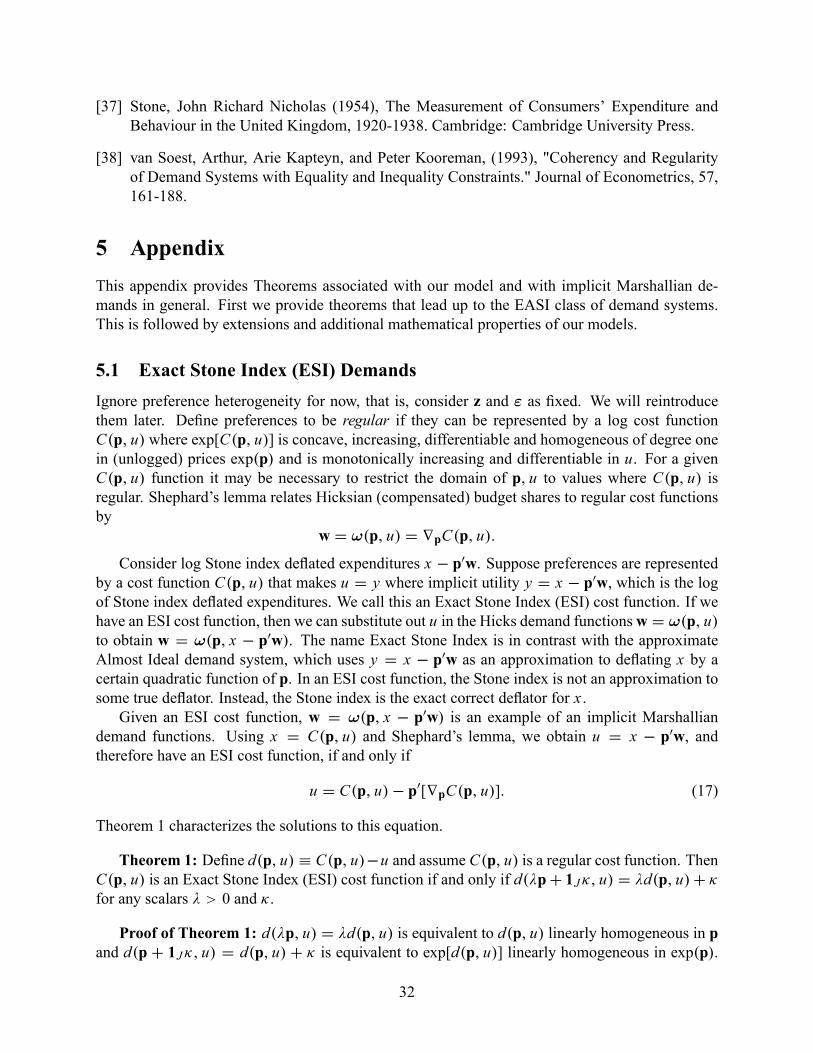
[37] Stone, John Richard Nicholas (1954), The Measurement of Consumers' Expenditure andBehaviour in the United Kingdom, 1920-1938. Cambridge: Cambridge University Press.

[38] van Soest, Arthur, Arie Kapteyn, and Peter Kooreman, (1993), "Coherency and Regularityof Demand Systems with Equality and Inequality Constraints." Journal of Econometrics, 57,161-188.

5 AppendixThis appendix provides Theorems associated with our model and with implicit Marshallian de-mands in general. First we provide theorems that lead up to the EASI class of demand systems.This is followed by extensions and additional mathematical properties of our models.

5.1 Exact Stone Index (ESI) DemandsIgnore preference heterogeneity for now, that is, consider z and " as �xed. We will reintroducethem later. De�ne preferences to be regular if they can be represented by a log cost functionC.p; u/ where exp[C.p; u/] is concave, increasing, differentiable and homogeneous of degree onein (unlogged) prices exp.p/ and is monotonically increasing and differentiable in u. For a givenC.p; u/ function it may be necessary to restrict the domain of p; u to values where C.p; u/ isregular. Shephard's lemma relates Hicksian (compensated) budget shares to regular cost functionsby

w D !.p; u/ D rpC.p; u/:

Consider log Stone index de�ated expenditures x � p0w. Suppose preferences are representedby a cost function C.p; u/ that makes u D y where implicit utility y D x � p0w, which is the logof Stone index de�ated expenditures. We call this an Exact Stone Index (ESI) cost function. If wehave an ESI cost function, then we can substitute out u in the Hicks demand functionsw D !.p; u/to obtain w D !.p; x � p0w/. The name Exact Stone Index is in contrast with the approximateAlmost Ideal demand system, which uses y D x � p0w as an approximation to de�ating x by acertain quadratic function of p. In an ESI cost function, the Stone index is not an approximation tosome true de�ator. Instead, the Stone index is the exact correct de�ator for x .Given an ESI cost function, w D !.p; x � p0w/ is an example of an implicit Marshallian

demand functions. Using x D C.p; u/ and Shephard's lemma, we obtain u D x � p0w, andtherefore have an ESI cost function, if and only if

u D C.p; u/� p0[rpC.p; u/]: (17)

Theorem 1 characterizes the solutions to this equation.

Theorem 1: De�ne d.p; u/ � C.p; u/�u and assume C.p; u/ is a regular cost function. ThenC.p; u/ is an Exact Stone Index (ESI) cost function if and only if d.�pC 1J�; u/ D �d.p; u/C �for any scalars � > 0 and � .

Proof of Theorem 1: d.�p; u/ D �d.p; u/ is equivalent to d.p; u/ linearly homogeneous in pand d.p C 1J�; u/ D d.p; u/ C � is equivalent to exp[d.p; u/] linearly homogeneous in exp.p/.

32

The latter condition is required by cost function regularity. For the former, given equation (17) wehave C.p; u/� u D p0

�rpC.p; u/

�. This is equivalent to d.p; u/ D p0

�rpd.p; u/

�, which by the

Euler Theorem shows that d.p; u/ is linearly homogeneous in p.

Theorem 1 can be equivalently stated as the requirement that exp[d.p; u/] be linearly homoge-neous in exp.p/, which follows from ordinary cost function homogeneity, and also that d.p; u/ belinearly homogeneous p, which makes u D x�p0w. A function d.p/ is de�ned to be, "translatableof degree c" if d.pC1J�/ D d.p; u/Cc� (see, e.g., Blackorby and Donaldson (1980)), so anotherway to state Theorem 1 is that C.p; u/ is an ESI cost function if and only if C.p; u/ � u is bothlinearly homogeneous in p and translatable of degree one in p.By ordinality of utility, instead of x � p0w D u, we could have de�ned Stone Index exactness

by x � p0w D h.u/ for any strictly monotonically increasing function h, and Theorem 1 wouldthen hold with d.p; u/ de�ned by C.p; u/ � h.u/ There is no gain in generality from doing so,because again by ordinality, C.p; u/� h.u/ has the same indifference curves, and hence the sameMarshallian and implicit Marshallian demand functions, as C.p; h�1.u// � u D eC.p; u/ � u.In this representation of the cost function (i.e., in this cardinalization of utility), we then obtainx � p0w D u as before.The following Corollary and theorem illustrates the restrictiveness of ESI demands.

Corollary 1: Assume C.p; u/ is an ESI cost function. Then Hicksian demands !.p; u/ DrpC.p; u/ are homogeneous of degree zero in p and in exp.p/.

Proof of Corollary 1: Homogeneity of degree zero in exp.p/ follows from ordinary cost func-tion regularity, and homogeneity of degree zero in p follows from the property that the derivativeof a linearly homogeneous function, in this case d.p; u/, must be homogeneous of degree zero.

Cost function regularity implies that Hicksian demands do not change when all prices are scaledby a constant factor. Corollary 1 shows that ESI requires that Hicksian demands also not changewhen all prices undergo the same power transformation, for example, when all prices are squared,and also rules out Hicksian demands that are linear in p. Relative prices can change dramati-cally when all prices are squared, so this additional homogeneity condition binds in economicallyimplausible ways.

Theorem 2: Consider the case where J D 2. Then d.�p1C�; �p2C�; u/ D �d.p1; p2; u/C�for any scalars � > 0 and � if and only if d.p1; p2; u/ D m.u/p1C[1�m.u/]p2 for some functionm.u/.

Proof of Theorem 2: Since d.�p1C�; �p2C�; u/ D �d.p1; p2; u/C� holds for any � and � ,let � D 1=.p2 � p1/ and � D �p1=.p2 � p1/ to obtain d.0; 1; u/ D

�d.p1; p2; u/= .p2 � p1/

���

p1= .p2 � p1/�. The theorem holds with m.u/ D 1� d.0; 1; u/.

Theorem 2 shows that with J D 2 goods, ESI cost functions must have the linear in p formC.p; u/ D u C p0m.u/ where m.u/ is a J�vector of functions that satisfy m.u/01J D 1. This isan ESI cost function for any J , but has the unattractive feature that it has Hicksian budget sharesm.u/ that are independent of p.

33

ESI cost functions having more than J D 2 goods can be nonlinear in p. One example is

C.p; u/ D u C p0m.u/C�p0M.u/p

�1=2where m.u/ is as above and M.u/ is a J by J symmetric matrix-valued function of u withM.u/1J D 0J . As this example shows, ESI log cost functions can be nonlinear in log prices,however, by Corollary 1 ESI log cost functions cannot be quadratic in log prices, and therefore ESIbudget shares cannot be linear in log prices.

5.2 Exact Af�ne Stone Index (EASI) DemandsAs shown in the previous section, ESI Hicks and implicit Marshallian budget shares must possessthe unattractive feature of not changing when all prices are squared, and also must either be inde-pendent of p or nonlinear in p. We can avoid these drawbacks by generalizing the expression forreal expenditures, thereby relaxing the homogeneity restrictions required by ESI demands. Specif-ically, instead of imposing the ESI restriction that some cardinalization of u equal x � p0w, de�neExact Af�ne Stone Index (EASI) cost functions to be cost functions that have the property that acardinalization of u exists that equals an af�ne transformation of x � p0w. In this cardinalizationu D y where implicit utility y is de�ned by y D

�x � p0w

�es.p/ �et.p/ for some functionses.p/andet.p/. For reasons that will be clear shortly, it is more convenient to express this relationship as

u D y Dx � p0w� t .p/1C s.p/

(18)

for some functions s.p/ and t .p/. We choose af�ne transforms for their simplicity, in particular,for now we wish to avoid having to solve nonlinear transformations to obtain cost functions (thenext section in this appendix discusses more general implicit Marshallian demand functions thatmay require nonlinear transformation).Equation (18) implies

x � u � p0w D t .p/C s.p/u;

and therefore any EASI cost function C.p; u/ must satisfy

C.p; u/� u � p0[rpC.p; u/] D t .p/C s.p/u (19)

The following two theorems characterize EASI cost functions, and hence the solutions to equation(19), and provide a convenient way to construct such functions.

Theorem 3: Assume C.p; u/ is regular. Let d.p; u/ � C.p; u/ � u. There exists functionst .p/ and s.p/ that make equation (18) hold, and hence make C.p; u/ an EASI cost function, ifand only if d.p C 1J�; u/ D d.p; u/ C � and r2ud.�p; u/ D �r2ud.p; u/ for any scalars � > 0and � . When equation (18) holds, the functions t .p/ and s.p/ satisfy t .p C 1J�/ D t .p/ C � ands.pC 1J�/ D s.p/C � .

Proof of Theorem 3: The condition that d.p C 1J�; u/ D d.p; u/ C � is equivalent toexp[d.p; u/] linearly homogeneous in exp.p/, which is required by cost function regularity. Equa-tion (19) is equivalent to d.p; u/�t .p/�s.p/u D p0

�rpd.p; u/

�. Taking derivatives of this expres-

34

sion with respect to u givesrud.p; u/�s.p/ D p0�rprud.p; u/

�, sor2ud.p; u/ D p0

�rpr2ud.p; u/

�,

which by the Euler Theorem shows thatr2ud.p; u/ is linearly homogeneous in p, that is,r2ud.�p; u/ D�r2ud.p; u/. In the other direction, if r2ud.p; u/ is linearly homogeneous then r2ud.p; u/ Dp0�rpr2ud.p; u/

�. Integrate this equation twice with respect to u (de�ning s.p/ be the constant of

integration for the �rst integration and t .p/ to be the constant of integration for the second integra-tion) and continue following the above steps in reverse to obtain equation (19). Given exactness,Equation (19) implies t .p/ C s.p/u D u � C.p; u/ C p0!.p; u/. Ordinary homogeneity of costfunctions and Hicksian demands requires that exp

�u � C.p; u/C p0!.p; u/

�be linearly homo-

geneous in exp.p/, so t .p/ C s.p/u must be linearly homogeneous in exp.p/. Since u can varyholding p �xed, this requires that t .p/ and s.p/ must each be linearly homogeneous in exp.p/ ,and therefore that t .pC 1J�/ D t .p/C � and s.pC 1J�/ D s.p/C � .

Theorem 4: Assume the function C.p; u/ satis�es the homogeneity conditions required to bean ESI log cost function as given by Theorem 1. Assume C.p; u/ D C.p; u/C T .p/C S.p/u is aregular log cost function. Then C.p; u/ is an EASI log cost function, so equation (18) holds, witht .p/ D T .p/� p0

�rpT .p/

�and s.p/ D S.p/� p0

�rpS.p/

�.

Proof of Theorem 4: C.p; u/ D C.p; u/C T .p/C S.p/u, so

C.p; u/� p0[rpC.p; u/] D C.p; u/� p0[rpC.p; u/]C T .p/� p0�rpT .p/

�C

S.p/u � p0�rpS.p/

�u

D u C T .p/� p0�rpT .p/

�C S.p/u � p0

�rpS.p/

�u

where the right side of the second equality follows from Stone index exactness for C.p; u/ fromTheorem 1. Comparing this equation to (19) proves the result.Now consider how observed variables z that affect preferences and how random unobserved

preference heterogeneity parameters " can be incorporated into the ESI and EASI cost functions.These cost functions are formulated above in terms of the functions C.p; u/, T .p/ and S.p/. In-corporation of observed heterogeneity is completely general in that there are no restrictions onhow observed characteristics z enter the ESI cost function C.p; u; z/ or the price functions T .p; z/and S.p; z/. However, the incorporation of unobserved heterogeneity is restricted by the fact thatimplicit utility y must be a function of observables only. This can be accomplished by letting Cdepend arbitrarily on " and having the price functions T .p; z/ and S.p; z/ be independent of ".The incorporation of both forms of heterogeneity then results in the general class of EASI costfunctions

C.p; u; z; "/ D C.p; u; z; "/C T .p; z/C S.p; z/u; (20)

where C is a regular ESI cost function and exp.T .p; z// and exp.S.p; z// are both homogeneousof degree zero in exp.p/. Based on equation (19) and Theorems 3 and 4, one very �exible choicefor C is C.p; u; z; "/ D u C p0m.u; z; "/, which allows for nonseparability with respect to theunobserved heterogeneity parameters ", and results in an EASI form

C.p; u; z; "/ D u C p0m.u; z; "/C T .p; z/C S.p; z/u: (21)

We will use this speci�cation for illustration in Theorems 6 through 8.Replacing m.u; z; "/ with m.u; z/ C " in equation (21) yields Hicksian (and hence implicit

35

Marshallian) budget shares that are additively separable in ", which is convenient for estimation.This results in the EASI cost function form

C.p; u; z; "/ D u C p0m.u; z/C T .p; z/C S.p; z/u C p0"; (22)

where 10Jm.u; z/ D 1 and 10J" D 0. We use this form as the basis for our empirical investigation

and for most discussion in the text.

5.3 General Cost Functions For Implicit Marshallian DemandsInstead of Stone index related constructions, we could more generally de�ne implicit utility by

y Dx � G.w;p; z/1C s.p; z/

(23)

for any de�ator function G. Setting y D u will then require

C.p; u; z/ D [1C s.p; z/]u C G.rpC.p; u; z/;p; z/ (24)

and the resulting implicit Marshallian demand functions are

w D !�p; z;

x � G.w;p; z/1C s.p; z/

�. (25)

where !.p; z; u/ D rpC.p; u; z/. At this level of generality, u D y is possible for almost any logcost function C.p; u; z/ even with s.p; z/ D 0 as the following Theorem shows.

Theorem 5: Assume C.p; u; z/ is regular. A suf�cient condition for existence of a func-tion G.w;p; z/ such that u D x � G.w;p; z/ is the existence of some scalar valued function ofrpC.p; u; z/ and p that is strictly monotonic in u.

Proof of Theorem 5: Let R be a scalar valued function of rpC.p; u; z/ and p that is strictlymonotonic in u. Since R.p; z;!.p; z; u// is strictly monotonic in u, it can be inverted to obtainu D S.p; z; R/, and we may de�ne a function G by G.w;p; z/ D C.p; S.p; z; R.w;p; z//z; / �S.p; z; R.w;p; z//.

Theorem 5 provides a very weak suf�cient condition for existence of implicit Marshallian de-mands w D !

�p; z; x � G.w;p; z/

�for some function G. For example, this condition is satis�ed

if any good or combination of goods has a budget share that is strictly increasing or strictly de-creasing in total expenditures (and hence in utility). Moreover, this condition is suf�cient but notnecessary, e.g., if preferences are homothetic so C.p; u; z/ D u C t .p; z/ for some function t , theneven though the suf�cient condition need not hold now, we can de�ne G.w;p; z/ D �t .p; z/ toobtain implicit marshallian demands. So the only kinds of situations where G might fail to exist iswhen all budget shares are independent of u for some, but not all, ranges of values of u.To give an example of Theorem 5, suppose that the Hicksian budget share function for good 1,

w1 D !1.p; z; u/, is invertible in u, so u D !�11 .p; z; w1/. Then a de�ator G that makes u D y isG.w;p; z/ D C.p; !�11 .p; z; w1/; z/� !

�11 .p; z; w1/.

36

The function G satisfying equation (24) is not unique, e.g., it can be freely translated by anordinal transformation of u, and in the previous example, different invertible budget shares could beused to obtain different expressions for G. For applications, the main point of implicit Marshalliandemands is not existence or uniqueness, but rather convenience for demand estimation, which iswhy this paper focuses on examples where G has a simple closed form, namely, a translation ofthe log Stone index.

5.4 Generalized EASI cost functionsA generalization of the EASI class of cost functions (22) is

x D C.p; u; z; "/ D u C c.p; z/0m.u; z; "/C T .p; z/C S.p; z/u (26)

where c.p; z/ is a J�vector valued function. The Hicksian budget shares for this class are

w D !.p; u; z; "/ D rpc.p; z/0m.u; z; "/CrpT .p; z/CrpS.p; z/u

Solving this expression for m.u; z; "/ and substituting the result into (26) gives

x D u C c.p; z/0�rpc.p; z/0

��1 �w�rpT .p; z/�rpS.p; z/u�C T .p; z/C S.p; z/uNow solve this expression for u and call the result y to get

y Dx � T .p; z/� c.p; z/0

�rpc.p; z/0

��1 �w�rpT .p; z/�1C S.p; z/� c.p; z/0

�rpc.p; z/0

��1rpS.p; z/

which we can write asy D

x � c.p; z/0w� t.p; z/1C s.p; z/

for appropriately de�ned functions t , s, and J�vector c, and with this de�nition of y we obtainimplicit Marshallian demands

w D rpc.p; z/0m.y/CrpT .p; z/CrpS.p; z/y

This is a generalization of EASI demands where y is an af�ne transform of x � c.p; z/0w insteadof an af�ne transform of x � p0w. This generalization is useful for the closure under unit scalingproperty discussed later, and could be used to introduce additional interactions among y, p, and zif required.

5.5 Global Regularity of EASI DemandsTheorem 6: Assume a log cost function in the general EASI form of equation (21). Suf�cient con-ditions for the cost function to be regular everywhere on the support of the data are 10Jm.u; z; "/ D1, exp

�T .p; z/

�and exp

�S.p; z

�/ homogeneous of degree zero in exp.p/, T .p; z/ and S.p; z/ con-

cave and differentiable in p, 1C inf�p0rum.u; z; "/

�> inf

�S.p; z/

�and inf.u/ > 0, where these

in�ma are over the supports of p; u; z; ".

37

Proof of Theorem 6: Homogeneity of the cost function follows from 10Jm.u; z; "/ D 1and homogeneity of exp T .p; z/ and exp S.p; z/. Concavity of T .p; z/ and S.p; z/ and havingu positive means that T .p; z/ C S.p; z/u is concave, which suf�ces for cost function concav-ity. For monotonicity ruC.p; u; z; "/ D 1 C p0rum.u; z; "/ C S.p; z/, which is positive given1C inf

�p0rum.u; z; "/

�> � inf

�S.p; z/

�.

By Theorem 6, EASI demands can be globally (i.e., over the entire supports of the data) regularif the functions T and S satisfy homogeneity and concavity conditions, and if T , S,m and the sup-ports of the data are suitably bounded. The suf�cient, though weaker than necessary, conditions inTheorem 6 include inf.u/ > 0 (recall that u here is expressed in the cardinalization that makes u Dy). This condition can always be satis�ed without loss of generality by suitably adjusting the unitsused to measure expenditures. To see this, de�ne K� D inf

�p0m.eu; z; "/C T .p; z/� where this in-

�mum is over all p; z; " on their support, and over alleu � 0. If K� exists, inf �S.p; z/� > �1 andinf.x/ > 0, then dividing the units expenditures are measured in by exp.K�/makes the log of theserescaled expenditures x satisfy inf.x/ > K�. This then suf�ces to make inf.u/ > 0 since, usingequation (2), u D

�x � p0m.u; z; "/C T .p; z/

�=�1C S.p; z/

�� [inf.x/� K�] =

�1C inf .S.p; z//

�>

0.In our empirical model based on the cost function (5), T .p; z/ and S.p; z/ satisfy homogene-

ity, are bounded given boundedness of prices and are concave ifPLlD0 zlAl and B are negative

semide�nite. Let cr D p0br , so boundedness of the support of p means that each cr lies insome interval. For monotonicity in our empirical model, assume y is everywhere positive, let�0 D

hinf.x/� sup

�p01 j �

PLlD0 zlp0Alp=2

�i=[1 C sup.�p0Bp/] and let �1 D sup.x/. It fol-

lows from equation (8) that �0 � y � �1. Let � D � inf�1C p0DzC p0Bp=2

�. Since cr D p0br ,

boundedness of the support of p means that each cr lies in some interval. Then the suf�cientmonotonicity condition in Theorem 6 is satis�ed if �c�1y�2C

P5rD0 crr yr�1 > � holds for all cr

on their supports and all y in the interval �0 � y � �1. In particular, if quantities are scaled so pis nonnegative, and recalling that �0 > 0, a suf�cient condition is existence of a �nite lower boundon the slope of every Engel curve at at every point. More generally, monotonicity requires thatdownward sloping portions of Engel curves for any good need to be suf�ciently offset by upwardslopes of other Engel curves.In practice, imposing the restrictions on parameter values that are suf�cient but not necessary

to guarantee global regularity of demand systems can induce undesirable restrictions on �exibility.See, e.g., Diewert and Wales (1987) and Ryan and Wales (1998). In our empirical application wetherefore follow the common practice of estimating without imposing the inequality constraintsassociated with regularity, and afterwards check for regularity in the neighborhood of the data.

5.6 Coherency, Invertibility, and the Distribution of ErrorsCoherency of a structural model is de�ned as the property that, for each value of the exogenousvariables and errors, there exists a unique corresponding value of the endogenous variables. Invert-ibility is the property that a unique value of errors is associated with each value of the endogenousand exogenous variables. Coherency is essentially the condition that the model is fully speci�ed,in the sense that the joint distribution of the endogenous variables is completely determined by thejoint distribution of the errors and exogenous variables. Invertibility is the condition that permits

38

uniquely recovering estimates of the errors given estimates of the model parameters. Since ourmodel takes the errors to be random utility parameters, we will require invertibility to do policyanalyses that depend upon these random utility parameters.In the demand system context (see, e.g., van Soest, Kapteyn, and Kooreman (1993), Brown

and Matzkin (1998) and Beckert and Blundell (2004)), coherency requires that a unique value ofbudget shares w be associated with each possible value of p; x; z; ", and invertibility requires thata unique value of errors " be associated with each possible value of p; x; z;w.

Theorem 7: Assume a log cost function in the EASI class (21) that is regular. Assume em Dm.u; z; "/ is invertible in ", so we may write " D m�1.u; z;em/. Then the resulting budget sharedemand functions are coherent and invertible.

Proof of Theorem 7: Invertibility of this class is established by observing that by equation (3)

" D m�1�y; z;w�

�rpT .p/

���rpS.p/

�y�

where y is given by equation (4). This uniquely de�nes " as a function of p; x; z;w. Coherencyfollows from C.p; u; z; "/ having all of the properties of a regular cost function, which ensuresexistence of Marshallian demands (treating " as preference parameters) and hence of a uniquevalue of w associated with each possible value of p; x; z; ", even though we do not have a closedform analytic expression for it.

Our functional form for empirical work, the cost function (5), satis�es the conditions of Theo-rem 7 assuming regularity holds on the support of p; x; z; " (which, e.g., is satis�ed given Theorem6). For that model m is invertible with, by equation (6), m�1.u; z;m/ D m �

�P5rD0 brur

��

Cz� Dzu. More generally, invertibility is satis�ed ifm.y; z; "/ D Bn.y; z/C" for any parametermatrix B and functions n.

For consistency of our estimator it was assumed that the distribution of " is mean independentof p; x; z, and our 3SLS estimator is ef�cient (relative to GMM) if " is homoskedastic. A suf�cientcondition for these to hold is that " be distributed independently of p; x; z. Having " independentof p is also appropriate for interpreting " as preference heterogeneity parameters. Having " bedistributed independently of p; x; z requires that the support of " not depend on p; x; z. Theorem7 does not impose this condition.

Theorem 8: Assume a log cost function in the EASI class (2). Then cost function regularity,the constraint that budget shares lie between zero and one, coherency, invertibility, and " distributedindependently of p; x; z can all hold simultaneously.

Proof of Theorem 8: Consider equation (2) cost functions with m.u; z; "/ D Bn.y; z/ C "for some matrix of parameters B and vector of functions n.y; z/. Our empirical model (5) is anexample of this form. Then

w D Bn.y; z/CrpT .p; z/CrpS.p; z/y C ". (27)

Consider bounding each element of Bn.y; z/CrpT .p; z/CrpS.p; z/y to lie inside some interval[� ; 1� � ] for every value of y in some positive interval [�0; �1] and for every value of p; z on their

39

support, where 0 < � < 1=2. The interval [�0; �1] can be made arbitrarily large by restrictingthe range of values n.y; z/ and rpS.p; z/ can take on. Let " be drawn from any distribution thatsatis�es "01J D 0 and has the absolute value of each element of " be less than � . Let x be drawnfrom any distribution that has support suf�ciently bounded to makeey de�ned by

ey D x � p0ew� T .p; z/C p0 �rpT .p; z/�1C S.p; z/� p0

�rpS.p; z/

� (28)

lie in [�0; �1] for every value of of p; z on their support and for every value of ew on the unitsimplex. Note that, as in the second part of Theorem 6, the units x is measured in can be adjustedto move the location of the support of x and hence ofey It then follows that y given by equation (4)will lie in [�0; �1], and then by construction w de�ned by equation (27) will lie in the unit simplex.Given the cost function (21) withm.u; z; "/ D Bn.u; z/C", and the assumptions already made

above, the remaining restrictions required for global regularity in Theorem 6 are 10JBn.u; z/ D 1,exp T .p; z/ and exp S.p; z/ homogeneous of degree zero in exp.p/, T .p; z/ and S.p; z/ concaveand differentiable in p, and 1 C inf

�p0Brun.u; z/

�> inf

�S.p; z/

�. Given that the support of u

lies inside an interval [�0; �1] for any value " can take on, we obtain global regularity for any " onits support as long as these conditions (which do not depend directly on ") hold for every p; z ontheir support and every u in the interval [�0; �1]. We then also obtain coherency and invertibility,because the conditions of Theorem 7 all hold for this example.

None of the conditions imposed in the construction of the cost function and the distribution of" in Theorem 8 con�ict with assumptions imposed for consistency of the the 3SLS estimates of ourexact, symmetry restricted empirically estimated EASI demand functions. For example, the proofof Theorem 8 allows each " to have conditional or unconditional mean zero, because it permits " tobe drawn from any distribution that satis�es "01J D 0 and has the absolute value of each elementof " be less than � , However, having " be distributed independently of p; x; z means that for anyvalue of p; x; z, the range of possible values of w is limited by the support of ". For example, ifthe support of " is such that each element of " is less than .1 in absolute value, and if for a givenp; x; zwe have each element of Bn.y; z/CrpT .p; z/CrpS.p; z/y lying between .2 and .8 for anyvalue of " (which, along with p; x; z determines y), then each element of w for consumers havingthis observed value of p; x; z must lie between .1 and .9 (though consumers with different valuesof p; x; z could have smaller or larger budget shares). This restriction on the conditional supportof w is a general feature of virtually all nontrivial demand systems that map demand errors intounobserved preference heterogeneity parameters, such as Brown and Matzkin (1998) and Matzkin(2005).Having " distributed independently of p; x; z implies conditional homoskedasticity of ". Brown

and Walker (1989) and Lewbel (2001) show that additive errors in Marshallian budget share de-mand systems must be heteroskedastic except under special circumstances (like homotheticity).Their results do not apply to the EASI model, because the EASI model has additive errors in im-plicit Marshallian (and hence in the Hicksian) budget share demand functions, rather than in theMarshallian budget share demand functions. Still, one might expect heteroskedastic errors, e.g.,empirical demands may have the property noted by Hildenbrand (1994) of variance increasing inx . This need not con�ict with the EASI model, or with regularity, coherence, or invertibility sinceall these conditions can be satis�ed ifm.y; z; "/ D Bn.y; z/CN.y; z; "/whereN is mean zero and

40

invertible in ", which would then generate implicit Marshallian budget errors given by N insteadof ".

5.7 The Rank of EASI Demand SystemsFor clarity, in this section the heterogeneity parameters z; " are held �xed, and so without lossof generality are omitted from the equations here. A demand system is de�ned to be exactlyaggregable if it has Marshallian demands of the form w D G.p/f.x/ for some matrix valuedfunction G.p/ and some vector valued function f.x/. Gorman (1981) proved that for any exactlyaggregable demand system that is derived from utility maximization, the maximum possible rankof the matrix G.p/ is three. Generalizing Gorman, Lewbel (1991) de�ned the rank of any demandsystem to be dimension of the space spanned by its Engel curves. This de�nition coincides withGorman's rank of G.p/ for the special case of exactly aggregable demands. Lewbel (1991) showsthat rank of the demand system corresponding to any cost function C.p; u/ equals the smallestinteger ` such that there exist functions g, �1,...,�`, where C.p; u/ D g[�1.p/; :::; �`.p/; u]. Themaximum possible rank of any demand system is the number of goods in the system minus one.It follows by inspection of equations (2) and (5) that EASI demands are not constrained to have

rank less than three, and can in fact have any rank, even when the EASI demands are linear in y.For example, for the reference type household the EASI demands we use for our empirical workhas the cost function C.p; u/ D p0

hP5rD0 brur

iC 12p0A0p C 1

2p0Bpu, which to minimize ` can

be written as C.p; u/ D�p0b0 C 1

2p0A0p

�C�p0b1 C 1

2p0Bp

�u C

P5rD2

�p0br

�ur , and so has rank

` D 6.

5.8 Shape Invariance and Equivalence ScalesShape-invariance is a property of demand functions that is relevant for the construction of equiv-alence scales, is convenient for semiparametric demand modelling, and has been found to at leastapproximately hold empirically in some data sets. See, e.g., Blundell and Lewbel (1991), andBlundell, Duncan and Pendakur (1998), Pendakur (1999), and Blundell, Chen, and Kristensen,(2003). Shape-invariance is satis�ed if and only if Marshallian budget shares are identical acrosshousehold types except for equation speci�c vertical translations and a horizontal translation thatis common across equations.In our notation, shape-invariance is satis�ed if and only if the log-cost function may be writ-

ten as C.p; u; z; "/ D f [p; h.u; z; "/] C G.p; z; "/. In this case, Hicks demands are given by!.p; u; z; "/ D rp f

�p; h.u; z; "/

�C rpG.p; z; "/. We may then invert C with respect to utility

to obtain indirect utility h.�; u; z; "/ D f �1��; x � G.p; z; "/

�and substituting this expression into

Hicks demands yields w D rp f�p; x � G.p; z; "/

�C rpG.p; z; "/. This structure for demands

may be very complex over x , but the characteristics z and " enter demands in a very simple way:they translate expenditure shares vertically by the J -vector rpG.p; z; "/ and horizontally by thescalar G.p; z; "/.De�ne an equivalence scale E as the ratio of costs of a household with characteristics z; "

and a household with reference characteristics 0L ; 0J , so that ln E.p; u; z; "/ D C.p; u; z; "/ �C.p; u; 0L ; 0J /. If demands are shape invariant and the untestable restriction that h.u; z; "/ D h.u/

41

holds then C.p; u; z; "/ D f�p; h.u/

�C G.p; z; "/ so

ln E.p; u; z; "/ D G.p; z; "/ (29)

and therefore the equivalence scale depends only on prices and characteristics, but not on the utilitylevel u. This property for E is called equivalence scale exactness (ESE) or independence-of-base(IB) by Blackorby and Donaldson (1993) and Lewbel (1989), respectively. Shape invariance is anecessary condition for IB/ESE.EASI models can be shape invariant and can satisfy IB/ESE. The cost function (21) satis�es

shape-invariance if and only if S is independent of z and the vector-function m is additively sepa-rable into a vector-function m1 that depends on utility only and a vector-function m2 that dependson characteristics z; " only. In this case, we have

C.p; u; z; "/ D u C p0m1.h.u; z; "//C p0m2.z; "/C T .p; z/C S.p/h.u; z; "/D

�u C p0m1.h.u; z; "//C S.p/h.u; z; "/

�C�p0m2.z; "/C T .p; z/

�:

This speci�cation also satis�es IB/ESE if it satis�es the additional, untestable restriction thath.u; z; "/ D h.u/.Shape-invariance is easily imposed on our empirically estimated model given by (5). In partic-

ular, that model has shape invariant demands if D D 0. However, with D D 0 the log equivalence-scale is given by ln E.p; u; z; "/ D p0 .CzC "/C 1

2PLlD1 zlp0Alp, which takes on a �xed value at

the base price vector, so ln E.0J ; u; z; "/ D 0. To relax this implausible restriction, one could adda term linear in z to the log-cost function with D D 0, so that

C.p; u; z; "/ D u C d0zC p0"5XrD0brur C CzC "

#C12

LXlD0zlp0AlpC

12p0Bpu; (30)

where d is a T�vector of parameters. The equivalence scale is then given by ln E.p; u; z; "/ Dd0zCp0 .CzC "/C 1

2PLlD1 zlp0Alp, which takes on the value d0z when evaluated at the base price

vector. In this version of the model, implicit utility y includes the constant term d0z and is givenby

y Dx � p0w� d0zC

PLlD0 zlp0Alp=2

1� p0Bp=2:

Other than this change in y, the demand functions are same as before, so the parameter vector denters the model only through y. Estimates of the model in this form are available on request fromthe authors.

5.9 Closure Under Unit ScalingA desirable feature of demand models is that they be closed under unit scaling, that is, that a changein the units that goods are measured in (or equivalently, a change in the base year or region whereprices are normalized to equal one) only changes the values of the parameters or functions thatde�ne the model, leaving predicted values and estimated elasticities unchanged. See, e.g., Pollakand Wales (1980), especially footnote 15. The AID system is closed under unit scaling. TheQuadratic AID of Banks, Blundell, and Lewbel (1997) is closed if the constant scalar parameter

42

a0 in that model is estimated, though in practice that parameter is usually �xed at some convenientvalue.The parametric models proposed in this paper are not closed under unit scaling. To close them,

we could replace p with p C k everywhere that p appears in equations (2), (3), and (4), or in ourempirically estimated model de�ned by equations (5), (8), and (9), where k is an additional J -vector of parameters to be estimated, with the free normalization k01J D 0. With the addition of zand " terms, these are examples of equation (26) with c.p/ D c.p/ D pC k.To check possible sensitivity of our empirical results to unit scaling, we tried to reestimate our

empirical model including the additional parameter vector k, but in every attempt k was eithercompletely insigni�cant or the model failed to converge. Also, reestimating the model (withoutk) after changing the base year and region had little effect on the estimates, leaving Engel curveshapes unchanged and altering elasticities by a few percent at most. Like the Quadratic AID modelwith a0 �xed, the parametric EASI models without k are approximately, though not exactly, closedunder unit scaling. Formally, the objective function used for parameter estimation is relatively �atin directions corresponding to changes in k.To see why the parametric EASI models as estimated are almost closed, consider the general

cost function

C.p; u; z; "/ D u C p0m.u; z; "/C p0 [A1 C A2h.u; z; "/]p=2 (31)

where h and the J -vector m are nonparametric functions. This cost function has demands that areclosed under unit scaling (up to possible inequality constraints on the nonparametric functions)because

C.pC k; u; z; "/ D u C .pC k/0m.u; z; "/C .pC k/0 [A1 C A2h.u; z; "/] .pC k/=2u� C p0m�.u�; z; "/C p0

�A1 C A2h�.u�; z; "/

�p=2

where u� D uCk0m.u; z; "/Ck0 [A1 C A2h.u; z; "/]k=2,m�.u�; z; "/ D m.u; z; "/C[A1 C A2h.u; z; "/]k,and h�.u�; z; "/ D h.u; z; "/, so by suitably rede�ning the functions m� and h�, adding k to thelog price vector is equivalent to ordinally transforming u, which leaves the resulting demand func-tions unchanged. This paper's parametric EASI models are special cases of the cost function (31),so they fail to be closed under unit scaling only because m� and h� need not be contained in thesame family of functional forms that are assumed for m and h. However, our �exible choice ofthese functions, particularly of m, means that m� and h� can be closely approximated by suitablechoice of parameterization of m and h, which explains the empirical �nding that the numericaleffects of violation of closure under unit scaling are very small.

5.10 Marshallian Elasticity CalculationsCost functions in the class of equation (21) have y given equation (8), so Marshallian demandfunctions w.p; x; z; "/ for these EASI models are implicitly given by

w.p; x; z; "/ D !�p;x � p0w.p; x; z; "/� p0A1p=2

1C p0A2p=2; z; "

�

43

Taking the total derivative of this expression with respect to any variable v gives

rvw.p; x; z; "/ D rv!.p; y; z; "/

C�r y!.p; y; z; "/

� �rv

�x � p0w� p0A1p=21C p0A2p=2

��

�x � p0rvw.p; x; z; "/

1C p0A2p=2

��and solving for the Marshallian semielasticity rvw.p; x; z; "/ yields

rvw.p; x; z; "/ D

"IJ �

�r y!.p; y; z; "/

�p0

1C p0A2p=2

#�1(32)"

rv!.p; y; z; "/C�r y!.p; y; z; "/

� "rv

x � p0w� p0A1p

21C p0A2p=2

!�

x1C p0A2p

2

##

where IJ is the J by J identity matrix. In particular, taking v to be x above shows that, afteralgebraic simpli�cation, the Marshallian semielasticity with respect to nominal expenditures x is

rxw.p; x; z; "/ D

IJ �

�r y!.p; y; z; "/

�p0

1C p0A2p=2

!�1 �.1� x/r y!.p; y; z; "/

1C p0A2p=2

�where r y!.p; y; z; "/ is given by equation (13). Equation (32) could also be evaluated taking v tobe p to obtain Marshallian price elasticities, but it is simpler to recover them from the Hicksian pelasticities (12) and the above Marshallian x elasticities using the Slutsky matrix

rp0w.p; x; z; "/ D rp0!.p; u; z; "/��rxw.p; x; z; "/

�!.p; y; z; "/0.

Finally, again using equation (32), the Marshallian semielasticity with respect to z is

rzw.p; x; z; "/ D

IJ �

�r y!.p; y; z; "/

�p0

1C p0A2p=2

!�1 �rz!.p; y; z; "/�

xr y!.p; y; z; "/1C p0A2p=2

�where r y!.p; y; z; "/ and rz!.p; y; z; "/ are given by equations (13) and (14).Some of the above elasticity expressions depend on " either directly or through w. Given

estimated model parameters, " for each consumer can be estimated as the model residuals (thedifference between �tted and observed w). We may therefore estimate mean elasticities in thepopulation by calculating the estimated elasticities for each individual in the sample, pluggingin their observed w or estimated " where needed, and averaging the result. Other features of thepopulation distribution of elasticities such as its median or variance can likewise be estimated fromthe corresponding empirical distribution.If Marshallian demands are of direct interest, evaluated at points other than those observed in

the sample, they can be obtained numerically by, e.g., numerically solving x D C.p; u; z; "/ for uand substituting the result into the Hicksian demand functions. However, as the above equationsshow, this will often not be necessary for evaluating the effects on demand or welfare of price,expenditure, or demographic changes.

44

Table 1: Data DescriptivesVariable Mean Std Dev Minimum Maximumbudget shares Food-at-Home 0.14 0.08 0.00 0.61

Food-Out 0.08 0.07 0.00 0.63Rent 0.37 0.12 0.01 0.89Household Oper 0.07 0.04 0.00 0.61Household Furneq 0.04 0.05 0.00 0.52Clothing 0.08 0.06 0.00 0.48Transport Oper 0.11 0.08 0.00 0.60Recreation 0.08 0.07 0.00 0.59Personal Care 0.03 0.02 0.00 0.21

log-prices Food-at-Home -0.05 0.43 -1.41 0.34Food-Out 0.04 0.49 -1.46 0.53Rent -0.08 0.40 -1.27 0.37Household Oper -0.06 0.45 -1.40 0.32Household Furneq -0.05 0.32 -0.94 0.20Clothing 0.04 0.35 -0.94 0.34Transport Oper -0.07 0.57 -1.53 0.57Recreation 0.01 0.40 -1.04 0.42Personal Care -0.03 0.38 -1.11 0.29

demographics age-40 0.71 11.89 -15.00 24.00male 0.51 0.50 0.00 1.00car-owner 0.42 0.49 0.00 1.00social asst 0.27 0.44 0.00 1.00time 88.99 8.73 69.00 99.00

log-expenditure x -0.11 0.59 -2.75 1.66(median-norm'd) x- p'w -0.07 0.44 -1.70 1.44

Table 2: Model Tests (Wald- or J-tests)model test of parameters df Test Stat p-valueasymmetric with symmetry Al=Al' for all l ; B=B' 196 241.8 0.014with y -1 , y 6

symmetry Al=Al' for all l 168 194.1 0.082symmetry B=B' 28 24.4 0.661exclusion B=0 64 82.5 0.060exclusion Al=0 for all l 384 636.0 0.000exclusion B=0, Al=0 for all l 448 999.7 0.000exclusion y -1

8 15.6 0.049exclusion y 6 8 20.6 0.008exclusion y 5

8 21.0 0.007exclusion y -1 , y 6

16 28.3 0.029exclusion y -1 , y 6 , y 5

24 75.5 0.000symmetric with exclusion B=0 36 51.7 0.043without y -1 , y 6

exclusion Al=0 for all l 216 646.2 0.000exclusion B=0, Al=0 for all l 252 710.6 0.000exclusion y 5 8 45.8 0.000non-quadratic Food-at-Home 3 16.9 0.001non-quadratic Food-Out 3 10.3 0.016non-quadratic Rent 3 94.4 0.000non-quadratic Household Oper 3 22.7 0.000non-quadratic Household Furneq 3 3.4 0.340non-quadratic Clothing 3 9.4 0.025non-quadratic Transport Oper 3 6.8 0.079non-quadratic Recreation 3 28.9 0.000overidentification J- test (with sym pz) 196 238.4 0.021overidentification J- test (with sym. pz, y -1 , y 6 ) 212 273.4 0.003

Table 3: Variation and Correlation of y Components (detrended variables)

Variable std dev y y (p'(w-e)) y -bar x- p'w x- p'w-bar p'e p'(w-e) p'Ap/2 p'Bp/2

y 0.4393 1.0000y (p'(w-e)) 0.4390 0.9988 1.0000

y -bar 0.4459 0.9984 0.9996 1.0000x -p'w 0.4387 1.0000 0.9988 0.9984 1.0000

x -p'w-bar 0.4452 0.9984 0.9996 1.0000 0.9984 1.0000p'e 0.0213 -0.0445 0.0041 0.0035 -0.0444 0.0035 1.0000

p'(w-e) 0.0716 0.0678 0.0672 0.0741 0.0685 0.0748 -0.0141 1.0000p'Ap/2 0.0018 0.0173 0.0165 0.0234 0.0134 0.0196 -0.0172 -0.2243 1.0000p'Bp/2 0.0011 -0.0123 -0.0141 -0.0122 -0.0140 -0.0140 -0.0371 -0.6439 0.4676 1.0000

Table 4: Compensated Price Effects, evaluated for reference type with median expenditure at base pricesOwn-Price Own-Price Own-PriceB element Slutsky Terms Quant Elast Food-in Food-Out Rent HH OperHH Furneq Clothing Tran Oper Recr

Food-at-Home 0.047 -0.137 -0.064 -0.025Std Err 0.063 0.045 0.347 0.045Food-Out -0.009 -0.120 -0.126 0.051 -0.025Std Err 0.068 0.037 0.346 0.033 0.037Rent 0.088 -0.164 0.528 -0.026 0.037 0.063Std Err 0.047 0.029 0.083 0.021 0.021 0.029Household Oper 0.044 -0.035 0.292 0.026 -0.002 -0.002 0.012Std Err 0.039 0.026 0.517 0.026 0.022 0.014 0.026Household Furneq 0.037 -0.034 -0.150 0.110 -0.043 0.028 -0.018 -0.005Std Err 0.114 0.058 1.937 0.035 0.032 0.021 0.026 0.058Clothing -0.050 -0.066 -0.063 -0.050 -0.001 -0.066 -0.025 -0.023 -0.008Std Err 0.060 0.046 0.734 0.030 0.032 0.020 0.024 0.038 0.046Transport Oper -0.006 -0.105 0.393 -0.023 -0.030 -0.019 -0.013 -0.034 0.053 0.038Std Err 0.035 0.020 0.115 0.021 0.019 0.016 0.017 0.021 0.019 0.020Recreation -0.030 -0.182 -1.191 -0.044 0.032 -0.021 0.034 -0.010 0.087 0.033 -0.106Std Err 0.093 0.053 0.635 0.034 0.032 0.023 0.025 0.045 0.037 0.022 0.053

Budget-share Semi-Elasticities

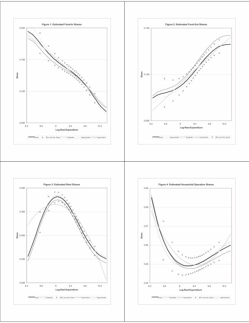
Figure 1: Estimated Food-In Shares

0.050

0.100

0.150

0.200

8.2 8.6 9 9.4 9.8 10.2

Log-Real-Expenditure

Sh

are

Exact 90% conf ints, Exact Quadratic Approximate Asymmetric

Figure 2: Estimated Food-Out Shares

0.050

0.100

0.150

8.2 8.6 9 9.4 9.8 10.2

Log-Real-Expenditure

Sh

are

Exact Approximate Quadratic Asymmetric 90% conf ints, Exact

Figure 3: Estimated Rent Shares

0.200

0.250

0.300

0.350

0.400

8.2 8.6 9 9.4 9.8 10.2

Log-Real-Expenditure

Sh

are

Exact Quadratic 90% conf ints, Exact Asymmetric Approximate

Figure 4: Estimated Household Operation Shares

0.04

0.05

0.06

0.07

0.08

0.09

8.2 8.6 9 9.4 9.8 10.2

Log-Real-Expenditure

Sh

are

Exact Quadratic Asymmetric 90% conf ints, Exact Approximate

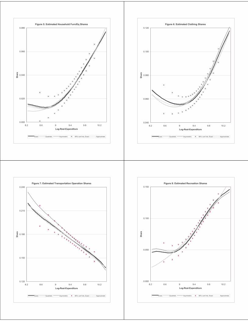
Figure 5: Estimated Household Furn/Eq Shares

0.000

0.020

0.040

0.060

0.080

8.2 8.6 9 9.4 9.8 10.2

Log-Real-Expenditure

Sh

are

Exact Quadratic Asymmetric 90% conf ints, Exact Approximate

Figure 6: Estimated Clothing Shares

0.040

0.060

0.080

0.100

0.120

8.2 8.6 9 9.4 9.8 10.2

Log-Real-Expenditure

Sh

are

Exact Quadratic Asymmetric 90% conf ints, Exact Approximate

Figure 7: Estimated Transportation Operation Shares

0.120

0.150

0.180

0.210

0.240

8.2 8.6 9 9.4 9.8 10.2

Log-Real-Expenditure

Sh

are

Exact Quadratic Asymmetric 90% conf ints, Exact Approximate

Figure 8: Estimated Recreation Shares

0.000

0.050

0.100

0.150

8.2 8.6 9 9.4 9.8 10.2

Log-Real-Expenditure

Sh

are

Exact Quadratic Asymmetric 90% conf ints, Exact Approximate

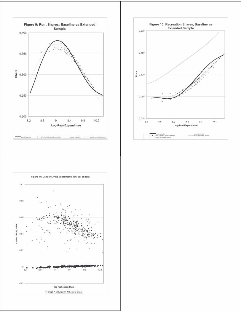
Figure 9: Rent Shares: Baseline vs Extended Sample

0.200

0.250

0.300

0.350

0.400

8.2 8.6 9 9.4 9.8 10.2

Log-Real-Expenditure

Sh

are

exact, baseline 90% conf ints, exact, extended exact, extended exact, extended, nopoor

Figure 10: Recreation Shares, Baseline vs Extended Sample

0.000

0.050

0.100

0.150

0.200

8.1 8.5 8.9 9.3 9.7 10.1

Log-Real-Expenditure

Sh

are

exact, baseline exact, extended90% conf ints, exact, extended exact, extended, no rentexact, extended, nopoor

Figure 11: Cost-of-Living Experiment: 15% tax on rent

-0.02

0

0.02

0.04

0.06

0.08

0.1

8.2 8.6 9 9.4 9.8 10.2

log real-expenditure

Co

st o

f L

ivin

g In

dex

COLI COLI (e=0) Second-Order