the trade-off theory and firm leverage
TRANSCRIPT

Stockholm School of Economics Bachelor Thesis Course 639 Accounting & Financial Management 2014
The Trade-off Theory and Firm Leverage Can the Trade-off theory explain the leverage development among Swedish listed firms?
Hampus Persson*
Joel Ridderström**
Abstract
This thesis aims to investigate if a dynamic application of the classic trade-off theory contributes
in explaining the leverage development among companies listed on the Swedish Stock Exchange.
After verifying inter-industry leverage differences, an industry comparing approach is applied to
contrast the explanatory power of the trade-off theory between industries. A partial adjustment
model is used to measure firms’ adjustment towards optimal leverage targets. Target leverage is
estimated in two ways. First, firm specific characteristics are used to explain firms’ optimal
leverage. Second, the industry standard is used as proxy for optimal capital structure. The
conclusions drawn are that leverage significantly differs across industries and that large- and mid-
cap firms’ leverage development can be explained by the trade-off theory. However, the trade-
off framework does not provide a comprehensive explanation of firms’ target leverage on
industry level.
Keywords: Trade-off theory, Dynamic framework, Firm characteristics, Leverage determinants, Industry standard Tutor: Walter Schuster Date: 19 May 2014

2
Table of contents
1 Introduction .......................................................................................................................................................... 3
1.1 Background .................................................................................................................................................. 3
1.2 Purpose of study ........................................................................................................................................... 4
1.3 Thesis research boundaries ........................................................................................................................... 6
1.4 Outline .......................................................................................................................................................... 6
2 Theory & previous research ................................................................................................................................. 7
2.1 Modigliani Miller & the efficient market ..................................................................................................... 7
2.2 Market imperfections and the trade-off theory ............................................................................................. 7
2.3 Theory development ..................................................................................................................................... 9
2.3.1 The dynamic model and firm characteristics ...................................................................................... 10
2.3.2 The industry standard ......................................................................................................................... 12
2.4 Previous research ........................................................................................................................................ 13
2.4.1 Firm characteristics and the dynamic framework ............................................................................... 13
2.4.2 Industry membership and capital structure ......................................................................................... 15
3 Hypothesizes and analysis logic matrix ............................................................................................................. 16
4 Method ............................................................................................................................................................... 18
4.1 The leverage measure ................................................................................................................................. 18
4.2 Industry classification ................................................................................................................................. 18
4.3 The sample ................................................................................................................................................. 19
4.4 Tests ........................................................................................................................................................... 20
4.4.1 Variance test ....................................................................................................................................... 20
4.4.2 Partial adjustment model .................................................................................................................... 22
4.5 Method critique .......................................................................................................................................... 26
5 Results and analysis ........................................................................................................................................... 28
5.1 Leverage development on the Swedish market .......................................................................................... 28
5.2 The partial adjustment model ..................................................................................................................... 30
5.2.1 Firm characteristic determinants ......................................................................................................... 30
5.2.2 Speed of adjustment ............................................................................................................................ 32
5.2.3 Industry standard as proxy for optimal leverage ................................................................................. 33
6 Discussion .......................................................................................................................................................... 34
6.1 Robustness .................................................................................................................................................. 36
6.2 Reliability, validity & generalizability ....................................................................................................... 39
7 Conclusions and suggestions for further research .............................................................................................. 39
8 Literature ............................................................................................................................................................ 41
8.1 Articles ....................................................................................................................................................... 41
8.2 Books .......................................................................................................................................................... 43
8.3 Internet sources .......................................................................................................................................... 43
8.3 Other sources .............................................................................................................................................. 44
9 Appendix ............................................................................................................................................................ 45

3
1 Introduction
Ever since Modigliani and Miller (1958) presented a theory of leverage irrelevance for firm
value in perfect markets, capital structure has been a widely debated subject. Modern theories
on optimal capital structure have found important links between leverage and firm value
(Schwartz, Aronson 1968; DeAngelo, Masulis 1980; Myers 1984). One theory that has
achieved recognition is the trade-off theory, saying that firms weight risks and benefits of
debt to find the optimal balance sheet (Myers 1984). In a Swedish context, the Corporate
Governance Code suggests that one of the primary tasks of a board is to monitor and decide
the firm’s leverage (Swedish Corporate Governance Board 2010).
Within the optimal capital structure theory, one line of research suggests that the choice of
leverage is set gradually in a dynamic environment. This viewpoint, known as the dynamic
framework, argues that investment and financing decisions are taken with flexibility over time
and are influenced by firm characteristics such as size, profitability, growth and volatility
(Byoun 2008; Mauer, Triantis 1994; Ozkan 2001; Titman, Wessels 1988). Also, further
studies within this field of research have found the industry as an explanatory factor of firms’
leverage development (Fischer, Heinkel & Zechner 1989; Frank, Goyal 2009).
Inspired by previous research, this thesis contributes to the capital structure debate by
examining if the leverage development among Swedish firms can be explained by the trade-
off theory in a dynamic framework. As part of the analysis we investigate if the industry
belonging plays a role when determining capital structure.
1.1 Background
The interplay between leverage and firm value has been a focal point in the world of finance
ever since the article “The cost of Capital, corporate finance and the theory of investment”
was published by Modigliani & Miller in the American Economic Review 1958. The
conclusion, that capital structure under the assumption of perfect markets is irrelevant for firm
value, made the two professors both worshiped and questioned.
What started as an article by two professors in the American Economic Review year 1958 has
ended up in numerous theories and concepts to understand firms’ capital structures. To get a
grip of the sprawling research field, two ways of thinking can be contrasted. First, one could
follow a pecking order theory, where the company is argued to choose internal before external

4
financing, without following any predetermined target debt-to-equity ratio. Secondly, one can
use a trade-off framework to explain the firm’s choice of capital structure. In the most basic
static trade-off framework, without recapitalization costs, the company is expected to weigh
the benefit from tax relief against the increased bankruptcy risk that comes with leverage. In
any period of time the company will obtain an optimal capital structure, resulting from a value
maximizing trade-off between these two factors. (Myers 1984)
Since the introduction of the two contrasting theories, research has led to confirmation as well
as rejection of both schools (Fama, French 2002; Ozkan 2001). Still, there is no conclusion
regarding which theory is the most relevant in explaining companies’ capital structures.
However, further development of the optimal capital structure theory has focused on
explaining firms’ leverage by using a dynamic framework. According to this later
development, firms over time gradually adjust their capital structures towards a target. In
presence of market imperfections such as recapitalization costs, deviations from the optimum
may not be perfectly adjusted for in each period, as assumed in static trade-off theory (Fischer
et al. 1989; Mauer, Triantis 1994).
Within both the static and dynamic framework, several firm specific characteristics have been
identified as determinants of a firm’s capital structure. Factors argued to be among the most
important are profitability, tangibility of assets, size, growth, depreciation and earnings
volatility (Frank, Goyal 2009; Rajan, Zingales 1995; Titman, Wessels 1988).
Further studies on firm specific characteristics have also found that companies in the same
industry have common leverage and adjust debt levels towards an industry standard. Scott and
Martin (1975) found evidence for persistent leverage differences between industries. Lev
(1969) developed a dynamic model illustrating the speed by which companies adjust certain
key ratios with respect to the industry average. Related studies have also found that share and
debt issuances are highly influenced by the company’s leverage relative to the industry
average (Billingsley, Smith & Lamy 1994; Hull 1999).
1.2 Purpose of study
Since Modigliani and Miller’s first article was published in 1958, there has been a constant
debate within the academic world about what determines a firm’s capital structure. The initial
static theories have been further developed into dynamic models, including a large number of

5
explanatory factors. However, there is still no academic consensus regarding how firms set
their capital structure (Fischer et al. 1989; Flannery, Rangan 2006; Myers 1984; Ozkan 2001).
Therefore, the purpose of this thesis is to investigate to which extent the capital structure
development on the Swedish stock market can be explained by the trade-off theory. Thus, the
research question reads out:
“Can the capital structure development among Swedish listed firms be explained by the
trade-off theory?”
We investigate the question by measuring if there is a gradual adjustment towards an optimal
leverage target, using a partial adjustment model within the dynamic framework (specified in
section 4.4.2). We use two proxies for the optimal leverage target. First, in accordance with
previous studies, we calculate the optimal leverage by regressing leverage ratios on firm
characteristics proved central in explaining capital structure (Byoun 2008; Flannery, Rangan
2006; Ozkan 2001). Second, we use the average industry leverage as a proxy for optimal
capital structure in the model. The industry proxy builds on previous research concluding that
there are persistent inter-industry differences and intra-industry similarities in leverage
(Bowen, Dale & Huber 1982; Schwartz, Aronson 1968; Scott, Martin 1975). In light of the
found industry differences, we investigate whether the explanatory power of the trade-off
theory differs between industries.
In addition to previous studies, our industry comparing approach contributes to further
understanding of the leverage development among Swedish listed firms. To the best of our
knowledge, previous studies on the subject have not contrasted the explanatory power of the
trade-off theory between industries on the Swedish market. Our findings may therefore
contribute with new valuable insights into how firms’ capital structure is determined in a
Swedish setting.
To validate the industry perspective and the usage of an industry standard as proxy for
optimal leverage, we first investigate if leverage differs between industries on the Swedish
stock market. Thereafter, tests are made on the relevance of the trade-off theory on the data.
The research question will be assessed through the work process stated below:

6
1. Analysis of leverage differences between industries on the Swedish stock market year
2002-2012
2. Analysis of the trade-off theory with an inter-industry perspective
a. By using a dynamic framework based on firm characteristics
b. By using a dynamic framework based on industry standards
1.3 Thesis research boundaries
This thesis aims to investigate if the leverage development among Swedish listed firms can be
explained by the trade-off theory. However, the study does not aim to isolate a single theory
as the answer to how a firm chooses to finance its operations. Several theories, not always
mutually exclusive, provide a wide range of frameworks that can be applied to explain firms’
leverage1. Given the limited scope of this thesis, we chose to focus on the trade-off theory and
its explanatory power alone. Also, we use the dynamic framework to measure if there is a
gradual correction among firms towards a leverage target in line with the trade-off theory.
The purpose is not to explain the potential refinancing costs associated with the speed of
correction.
The leverage level is compared between industries to find out if there are persistent industry
differences. The comparison is intended to justify the inter-industry perspective and the
industry standard proxy. The goal is not to further investigate why there are inter-industry
differences or what implication these differences have on firms’ operations. Furthermore, the
study is conducted in a Swedish setting, only considering firms listed on the small-, mid- and
large-cap exchanges on NASDAQ OMX Stockholm. Therefore, we are not aiming to give
any general conclusions in an international context.
1.4 Outline
The thesis is presented in the following order. In chapter 2 we present theory and previous
research within the subject of optimal capital structure. In section 3 we introduce our analysis
logic and hypothesises intended to test. In section 4, a description of the sample and methods
used to test the stated hypothesises are presented. In section 5, the found results are reported
and investigated. In section 6, the results are discussed and tested for robustness. In Section 7,
we present our conclusions and give some suggestions for further research on the topic.
1Hovakimian, Opler and Titman (2001) suggest that firms may operate with leverage targets in accordance with the-trade off theory but still
prefer internal to financing to external financing, explained by the pecking order framework.

7
2 Theory & previous research
2.1 Modigliani Miller & the efficient market
The most fundamental theory within the field of capital structure was presented in 1958 by
the two professors Modigliani and Miller. Assuming an efficient market (absence of taxes,
bankruptcy costs, agency costs and asymmetric information), the theory suggests that the
capital structure plays no role for the value of the firm. The theory builds upon two proposals,
stated below.
1. The market value of any firm is independent of its capital structure and is given by capitalizing its
expected return at the rate appropriate to its class. (MM, 1958)
2. The expected yield of a share of stock is equal to the appropriate capitalization rate for a pure
equity stream in the class, plus a premium related to financial risk (MM, 1958)
The first proposal is illustrated by comparing two firms, one levered and one unlevered.
Given that the two firms generate the same cash flow streams, they must be valued at the
same price. If this rule is violated, the arbitrage opportunity will make investors act and
correct the mispricing. This also implies that the cost of capital for any chosen combination of
debt and equity in perfect capital markets will be equal to the cost of capital for the unlevered
firm. The second proposal illustrates how the cost of capital will be unaffected by the
combination of debt and equity financing. Increasing debt will lead to a rising cost of equity,
related to a risk premium, and an unchanged unlevered equity cost of capital. This keeps the
firm value constant and unaffected by changed debt-to-equity ratios (Berk, DeMarzo 2011).
2.2 Market imperfections and the trade-off theory
After the first theory in 1958, Modigliani & Miller wrote several articles on the subject of
capital structure (Miller, Modigliani 1961; Miller, Modigliani 1963; Miller, Modigliani 1966).
The professors again gained much attention when presenting a correction paper to the original
theory, relaxing the no tax assumption. Under the new assumptions, a tax advantage to debt
financing arises since interest expenses are tax deductible. Higher leverage leads to increased
interest costs. The tax rate multiplied by the interest cost will be sheltered from the required
tax payment. This benefit of debt is called a tax shield and leads to an optimal capital
structure fully financed by debt (Baxter 1967; Modigliani, Miller 1963).
The correction paper presented in 1963, arguing that a tax shield provided by tax-deductible
interest expenses creates an optimal capital structure fully financed by debt, was discarded as

8
unrealistic by numerous later researches. First, debt financing is often conditional on a certain
equity stake in the company (Baxter 1967; Solomon 1963). Second, empirical evidence shows
that companies in practice only are levered to a fraction of total firm value (Kim 1978).
Clearly, some important variables where left out when allowing for market imperfections.
In reality, an important consequence of debt financing, and a missing element in Modigliani
and Millers framework, is the increased bankruptcy risk (Baxter 1967; Van Horne 1974).
Since debt financing leads to fixed payment claims, increased leverage also leads to higher
bankruptcy risk and increased borrowing costs. Increased cost due to bankruptcy risk and
financial distress will at a certain level offset the positive effect from leverage and reduce the
firm value. The approach to weight pros and cons of leverage has developed into a well-
known line of research called the trade-off theory (Berk, DeMarzo 2011). From this
perspective, a levered company reaches maximized firm value when the marginal gain from
the tax shield is exactly offset by the increased cost of financial distress. The earliest trade-off
theory can be seen as a static framework where every firm holds investment plans constant
and where the optimal trade-off is at one fixed point. Assuming no refinancing costs, a firm
that is off the optimal point will immediately adjust perfectly towards the value-maximizing
target (Myers 1984).
What is described as an optimal capital structure in theory demands a number of assumptions
in reality. To determine the present value of financial distress costs, several aspects need to be
considered. First, the risk of bankruptcy or financial distress must be estimated. Second, the
costs in case of distress need to be approximated. Also, the discount rate of the estimated
bankruptcy- or distress costs must be calculated (Berk, DeMarzo 2011). Due to the real-world
complexity, Miller (1977) argued that no firm can have enough information of the business
outlook to provide any evidence of the described trade-off optimization. Miller also
challenged the trade-off theory by showing that under certain conditions the tax advantage of
debt financing is counterbalanced by the tax disadvantage of debt at a personal tax level.
Since Millers’ evidence against some of the tax advantages from debt, the research has
continued in trying to understand how and why firms end up with a certain capital structure.
The agency theory takes a managerial approach in explaining how companies act. The theory
can be seen as an extension of the trade-off framework (Berk, DeMarzo 2011; Frank, Goyal
2009). From an agency perspective, costs and benefits occur when there is a conflict of

9
interest between sponsors of the firm. Executives are tempted to run the company in a way
that maximizes their personal wealth. The shareholders wish to maximize shareholder value
and the firm’s creditors want the firm to be solvent. Since executives often also are owners of
the firm, the main focus tends to end up in value maximization of the firm’s equity,
sometimes at cost of total firm value and creditors interest. One example of an agency related
cost rising from the conflict of interest is excessive risk taking. In a firm financed by a large
portion of debt, shareholders may consider excessively risky projects since a potential failure
mainly affects the debt holders. This can also lead to an asset substitution meaning that high-
risk assets substitute low risk assets, increasing the overall risk profile of the firm. Debt
overhang and underinvestment are two other agency related costs that need to be considered.
In a firm with large portions of debt, debt holders will capture most of the profit from a
project, leaving shareholders with low returns and no incentives to take on promising projects.
(Berk, DeMarzo 2011)
Examples of agency related benefits of debt are concentration of ownership and increased
commitment. Keeping the shareholder base intact will allow the initial owners with high
commitment to keep the business on track without any disturbing co-owners following
different strategies or agendas. Also, debt can work as a disciplinary factor. Creditors demand
fixed payments, which increases the risk of financial distress. The uncertainty leads to higher
pressure on the executives to generate profitability. (Berk, DeMarzo 2011)
2.3 Theory development
The optimal capital structure theory, introduced by Modigliani & Miller 1958, has led to the
conclusion that in perfect capital markets, the capital structure is irrelevant for firm value
(Myers 1984). However, in reality the world is not frictionless and imperfections seem to play
a significant role in a firm’s choice of capital structure. The trade-off theory, extended with
the agency perspective, establishes a relationship between the levered and unlevered firm
through four influencing factors. Together, the interest tax shield, bankruptcy costs, agency
related costs and agency related benefits build the bridge between the value of an unlevered
and a levered firm. The optimal capital structure is reached when a company finds the value-
maximized combination of these four factors (Berk, DeMarzo 2011).
What may look like an obvious outcome in theory is not as clear in reality. Studies have
discarded the static trade-off theory and found that firms in reality, due to market

10
imperfections such as refinancing costs, seem to set leverage targets in a dynamic way
without a fixed optimum or a perfect adjustment in each period (Fischer et al. 1989; Mauer,
Triantis 1994). If the static framework presented by the initial trade-off theory is not
applicable but firms set their targets in a dynamic setting, the question remains how such a
dynamic setting works and which factors that in practice determine the described theoretical
optimum.
2.3.1 The dynamic model and firm characteristics
Myers (1984) argued that if market imperfections such as adjustment costs are included in the
trade-off framework, a lag effect is expected where firms gradually adjusts towards a target. A
consequence of adjustment costs is that firms in several time periods can deviate from the
optimal capital structure. However, the static framework assumes the adjustment cost to be
negligible and that the company in a each period reaches the optimum.
Fischer, Heinkel and Zechner (1989) included recapitalization costs in the equation and
reached new conclusions. By developing a multi period model of dynamic capital structure
choices, the authors found that firms follow an optimal dynamic capital structure policy. This
policy depends on the conventional benefits and costs of debt financing such as tax
advantages and bankruptcy costs, but also on the costs of recapitalization. Due to
recapitalization costs, firms may allow the ratio to be in a range around the optimum
described in the static trade-off theory. The presented dynamic framework argues that similar
firms could have different leverage ratios at any point of time but also that similar firms
gradually adjust in the same direction.
Within the trade-off framework, previous research has found several firm specific variables as
determinants of optimum leverage. Firm size, tangibility of assets, growth, volatility,
profitability and depreciation are variables that consistently re-appear as the most important
determinants in the research (e.g. Bauer 2004; Bradley, Jarrell & Kim 1983; Kester 1986).
Firm size is predicted to have positive impact on leverage within the trade-off theory. This
relationship is expected due to an established negative correlation between firm size and
bankruptcy related costs (Warner 1977). An explanation to the negative correlation is that
large firms often have more diversified businesses than small companies. A wider business
model generates more stable cash flow streams, which leads to a lower rate of bankruptcy,

11
resulting in better borrowing terms and higher optimal leverage (Margaritis, Psillaki 2007;
Rajan, Zingales 1995). Also, the agency related costs described in section 2.2 are predicted to
be lower among large firms compared to small companies (Antoniou, Guney & Paudyal
2008).
In accordance with firm size, tangibility of assets is predicted positively correlated with
leverage within the trade-off framework. A negative effect of tangibility on bankruptcy risk
and agency-related costs explains the predicted positive correlation. Since tangible assets are
considered easier to value and sell than intangible assets, a firm with high rate of tangibility
will find it easier to survive in times of financial distress. A high rate of tangible assets also
makes it harder to conduct the asset substitution, described in section 2.2 (Frank, Goyal
2009).
The static trade-off theory predicts positive correlation between profitability and leverage.
Profitability is associated with high stock returns, low bankruptcy risk and therefore low
borrowing costs. Low borrowing costs together with the tax shield advantage discussed in
section 2.2 increases the incentives to take on debt (Margaritis, Psillaki 2007). The increased
discipline that comes with debt, described by the agency theory, is also argued to keep
pressure on executives to perform in an already profitable firm (Frank, Goyal 2009).
However, within a dynamic framework, the positive relationship between profitability and
leverage may be dampened due to market frictions such as refinancing costs (Strebulaev
2007). This reasoning is further backed by the mechanical relationship between retained
earnings and solidity (Flannery, Rangan 2006).
Volatile earnings and high growth are considered to be factors increasing the risk profile of a
firm and thus lead to lower optimal leverage levels. Unpredictable earnings make it harder to
maintain an appropriate debt level from a tax-shield perspective. It becomes hard to match the
tax-deductible interest cost with the volatile earnings and a mismatch could lead to financial
distress (Titman, Wessels 1988). Fast growing firms are more exposed to the described
agency-related costs than mature firms. High growth also leads to increased bankruptcy risk
and thus higher cost of financial distress, which should lead to a lower optimal leverage
(Frank, Goyal 2009).

12
Depreciation is predicted negatively correlated with leverage within the trade-off theory. A
higher rate of depreciation will lead to tax deductions comparable to the tax shield provided
by increased debt, which lowers the incentives to take on debt (DeAngelo, Masulis 1980).
Worth noticing is that the expected leverage effect from the variables are different depending
on which theoretical framework that is used. For example, the Pecking order theory stands in
contrast to the trade-off theory when it comes to leverage effects from different variables. In
fact, according to the Pecking order theory, a majority of the variables are predicted to have
the opposite effect on leverage to the above described (Frank, Goyal 2009; Myers 1984;
Titman, Wessels 1988). In addition, the depreciation effect on leverage is assumed positive
when following the secured debt hypothesis, presented by Scott (1977). According to this
hypothesis, a high level of depreciation is a result of high tangibility, which should lead to
better borrowing terms and higher debt levels (Boquist, Moore 1984). Even though the focus
in this thesis is on the trade-off framework, we find it important to address the double-faced
character of the variables.
2.3.2 The industry standard
Research has also found a significant relationship between firms’ characteristics, their
leverage ratios and industry classification. The argument is that firms within the same
industry tend to have similar firm characteristics, facing the same business environment and
therefore also aim for similar capital structures (Bradley et al. 1983; Remmers, Stonehill,
Wright & Beekhuisen 1974). From a theoretical perspective, the relationship can be explained
by sub-dividing risk into operating and financial components, as done in equation 1 below.
(1)
Return on equity ( ) is a function of return on total capital and leverage (
.
Operating risk is defined as the variability in return on total capital. This risk component is
associated with investments, production and price policies. The financial risk component is
risk related to debt and financial leverage (Johansson 1983). Mandelker and Rhee (1984) and
Marsh (1982) have found a negative correlation between operating and financial risk. Firms in
the same industry face similar business environments and are therefore considered having
1 2
1: Operating Risk
2: Financial Risk

13
comparable operating risks (Berk, DeMarzo 2011). This should lead to intra-industry
similarities and inter-industry differences in capital structure. For example, firms within
sectors such as Real Estate and Construction & Materials are expected to have lower
operating risk and thus higher leverage ratios than firms within areas such as Software and
Biotechnology (Bougheas 2004). The finding that firms within the same business tend to aim
for similar capital structures have led to an application of the industry standard as proxy for
optimal leverage in several well recognized studies on capital structure (Bowen et al. 1982;
Fischer et al. 1989; Hull 1999).
2.4 Previous research
The dynamic framework has been used to test the trade-off theory in multiple studies and
settings. Several studies have also investigated firm characteristic leverage effects and what
role the industry plays in the framework.
2.4.1 Firm characteristics and the dynamic framework
The predicted firm characteristic leverage effects, described in section 2.3.1, have been
investigated by numerous empirical studies. A selection of previous findings is presented in
table 1 below.
Table 1 – Articles investigating firm specific determinants of leverage
A majority of the studies have found that the independent variables generally affect leverage
in line with the predictions in the trade-off framework. However, research has also found
some interesting contradicting results. Kester (1986) found a positive relationship between
Tangibility Depreciation Growth Size Volatility Profitability R&D Industry2)
Bradley et al. (1983) + - - x LTD/(E (MV) + TD (BV))
Bauer (2004) - - - + - xTL/TA (BV &MV), TD/TA (BV &
MV)
Friend and Lang (1988) + + - - TD/TA (BV)
Kester (1986) + - - TD/TA (BV & MV), ND/E (BV & MV)
Kim & Sorensen (1986) - + TD/E (MV)
Marsh (1982) + + LTD/CE (BV), STD/TD (BV)
Titman & Wessels (1988) + - - - - - - x TD/TA3)
Margaritis and Psillaki (2007) + + LTD/TA (BV), STD/TA (BV)
Ozkan (2001) - - + - TD/TA (BV)
Frank and Goyal (2009) + - + +/- x4 TD/TA (MV &BV), LTD/TA (BV &
MV)
Byoun (2008) - - +TD/TA (BV & MV), LTD/TA (BV &
MV)
Prediction by the trade-off framework + - - + - + -1)
LTD = Long Term Debt, STD = Short Term Debt, TD = Total Debt, ND = Net Debt, TL = Total Liabilities, TA = Total Assets, E = Equity, CE = Capital Employed, BV = Book Value, MV = Market Value
2) Industries contrasted by dummy variables, therefore no unanimous sign presented
3) Numerous other leverage ratios tested
4Positive relation found between mean industry leverage and firm leverage
Article Tested leverage ratios1)Effect on leverage from Independent variables

14
growth and leverage when comparing U.S. and Japanese manufacturing corporations.
Investigating U.S. firms, Titman and Wessels (1988) found contradicting results for firm size.
This effect was especially strong when short-term debt was used as dependent variable. The
outcome was explained by substantial refinancing costs for small firms with low bargaining
power when issuing long-term debt, leading to higher short-term leverage ratios. Bauer (2004)
investigated the Czech Republic market and found a negative relationship between tangibility
and leverage, lacking any theoretical support. Bradley, Jarrell and Kim (1983) and Titman and
Wessels (1988) highlighted R&D spending as an additional important variable within
technology dependent sectors. Kim & Sorensen (1986) found contradicting results when
measuring the earnings volatility effect on leverage. Even though the results differed from the
predicted outcomes, spill over effects from the agency theory were argued to lead to a positive
relation, still in accordance with the trade-off framework. The authors reasoning illustrate the
complexity of the subject and the potential weakness of the somewhat simplified predictions
presented in our theoretical framework.
The authors verify the scattered results by claiming that other theories better explain some of
the variables’ leverage effect than the trade-off theory. Frank and Goyal (2009) found the
negative relationship between profitability and debt to be more in line with the pecking order
theory. Bradley et al. (1983) rejected the predicted negative relation between depreciation and
leverage by referring to the hypothesis of secured debt (Scott 1977). Nevertheless, a general
conclusion among the studies is that the trade-off theory to a high degree explains the firm
characteristics’ effect on leverage. Frank and Goyal (2009) summarize that no available
theory fully can explain firms leverage on the U.S. market but that the trade-off theory still
provides the most comprehensive framework in understanding firms’ capital structure.
A conclusion among studies investigating the trade-off theory in a dynamic framework is that
firms over time adjust leverage ratios towards an optimum determined by firm characteristics.
However, the discovered adjustment speed towards the optimum differs among studies.
Ozkan (2001) revealed fast adjustments toward leverage targets on the UK market2. Later,
Antoniou, Guney and Paudyal (2008) confirmed the fast adjustment speeds among European
and U.S. firms. Flannery and Rangan (2006) identified slower adjustments among U.S. firms,
2 Above 50% of the deviation was corrected towards the target in each time period.

15
robust for size differences3. Fama and French (2002) found even slower correction speeds
among firms on the U.S. market4
. All studies investigated the trade-off theory by
specifications of a partial adjustment model, later described in section 4.4.2. High adjustment
speeds are said to imply low refinancing costs while slow adjustments are associated with
higher refinancing costs, preventing firms from perfect adjustments in line with the trade-off
theory (Fama, French 2002; Ozkan 2001).
2.4.2 Industry membership and capital structure
The validity of an industry standard as proxy for optimal capital structure builds on the
assumption that there are similar leverage levels within industries and different leverage
levels between industries. If this condition is not fulfilled, the industry standard is said to lack
explanatory power of firms’ leverage (Flannery, Rangan 2006). Below, a brief summary of
studies on industry differences is provided.
Table 2 – Previous studies on industry differences in leverage
Schwartz and Aronson (1968) found early evidence for industry differences in leverage ratios
in the U.S. The findings where criticised as biased since several of the investigated industries
where regulated, leading to forced variances. However, including numerous unregulated
industries, Scott and Martin (1975) found further evidence for persistent differences. Bowen
Daley and Huber (1982) added robustness to the discovered industry differences using more
granular sector classifications (using four digit SIC codes). By also applying pairwise tests,
the authors verified that several of the studied sectors differed from each other. However, not
all previous findings agree on the results. In an international study, Remmers, Stonehill,
Wright and Beekhuisen (1974) rejected the industry standard as a good proxy for business
risk and optimal leverage when no significant inter-industry differences in leverage were
found. MacKay and Phillips (2005) also provided evidence for larger intra-industry than inter-
3 Between 20 and 30% of the deviation from the target was found corrected in each time period. A slight inversed relationship between size
and adjustment speed was found. 4 Correction speeds measured between 10 and 20%.
Authors Industries tested Country
Schwartz & Aronson Railroads, Utilities Electric & Gas, Mining, Industrials U.S
Scott & Martin Aerospace, Auto Parts and Accessories, Chemicals, Drugs, Glass producers & Container, Machinery &
Machinery Tools, Mining, Non-ferrous Metals, Oil, Paper & Forest Products, Retail Stores, SteelU.S
Bowen, Daley & HuberTextile Products, Chemicals, Oil-Integrated Domestic, Steel, Auto Parts & Accessories, Aerospace, Air
Transportation, Retail Department Stores, Retail Food ChainsU.S
Remmers et al* Appliances and Electronics, Chemicals, Farm and Industrial Machinery, Food, Metal Manufacturing, Metal
Products, Motor Vehicles and Parts, Paper and Wood Products, Petroleum Refining
France, Japan, Netherlands,
Norway, U.S
MacKay and Phillips315 competitive manufacturing firms where included in an international study to find potential inter-industry
differencesU.S
*Tests outside the U.S only including Electrical, Paper, Food and Chemicals industries

16
industry variation in leverage in the U.S. The contrasting results make an assessment of the
Swedish environment necessary before applying the proxy.
Also when testing the proxy for optimal capital structure, previous studies have reached
contrasting conclusions. Using a partial adjustment model, Lev (1969) found significant
convergence towards an industry standard for numerous leverage measures. Using a non-
parametric approach, Bowen et al. (1982) added further robustness to the proxy. On the
contrary, MacKay and Phillips (2005) and Flannery and Rangan (2006) rejected the proxy as
substitute for firm specific targets.
3 Hypothesizes and analysis logic matrix
We follow the outline stated in section 1.2 to answer our research question. First, we map the
leverage development among listed firms on the Swedish stock market to investigate if there
are persistent industry leverage differences. This is done to confirm or reject the connection
between industry belonging and capital structure. Confirmation or rejection will be made
through tests of the null hypothesis with the belonging two-sided alternative hypothesis
, stated below.
The average leverage ratio does not differ between industries over time
The average leverage ratio does differ between industries over time
The rule used is to reject if any industry differences are found. After rejecting or
confirming the hypothesis regarding industry differences, an analysis is conducted to
investigate whether the companies in our sample over time adjust leverage in line with the
trade-off theory. The analysis is conducted through tests of the null hypothesis with the
belonging alternative hypothesis , stated below. Since we are taking an industry
perspective in the analysis, after initial tests on the whole sample, industry comparisons are
made to find if the outcome of the test of is dependent on industry belonging.
Companies on the Swedish market do not adjust the leverage ratio in
accordance with the trade-off theory
Companies on the Swedish market do adjust the leverage ratio in accordance
with the trade-off theory

17
Industry Level
Whole Sample
Step 1Firm Specific Target
Test on whole sample with firmspecific target
Industry comparison with firmspecific target
Test on whole sample withindustry proxy as target
Industry comparison withindustry proxy as target
Step 2Industry Standard
Conditional on rejection of
The test of the null hypothesis on the whole sample and with an industry perspective is
done in two steps. First, a dynamic framework based on firm characteristics is used to
determine the optimal leverage level and to investigate if any movement towards a target can
be found in accordance with the trade-off theory. Second, in the same setting, the industry
standard as proxy for optimal leverage is used to investigate firms’ adjustment. However, the
rational for using the proxy for optimal leverage is conditional on rejection of the null
hypothesis .
To summarize the analysis logic of our study, a two by two matrix is used, illustrated in figure
1. In step 1, the null hypothesis is tested with a target based on firm characteristics ( ).
Industry comparisons are made of the results after an initial test on the whole sample has been
conducted. Thereafter, conditional on rejection of , step 2 of the analysis is initiated. Each
industry’s yearly mean leverage ratio ( ) is used as target to again test the null hypothesis
and contrast the industries.
Figure 1 – Analysis logic matrix
In step 1, we reject the null hypothesis if a majority of the significant firm characteristics
affect the estimated target ( ) in line with the trade-off theory and if significant adjustment
towards the targets is found. In step 2, the target ( ) is assumed in line with the trade-off
theory. In this case, the rejection rule is only based on a significant adjustment speed towards
the target.
18
4 Method
4.1 The leverage measure
The theoretical framework has been used when choosing which leverage ratio to investigate.
The leverage components of interest are the ones affecting the optimal capital structure
according to the trade-off theory. Bankruptcy costs and tax shields are dependent on tax-
deductible interest-bearing debt that lowers tax payments and increases risk through fixed
payment claims. A first constraint is therefore to focus on interest-bearing debt.
When defining interest-bearing debt, book value or market value can be used. There are
advantages and drawbacks with both approaches. Myers (1977) and Graham and Harvey
(2001) argue that book value of debt is the most accurate. Since the capital markets can be
volatile, executives are claimed to put little value in market-based ratios. The argument for
market leverage being superior to book values is that the book value of equity works as
residual to make the financial statements balance, leading to skewed leverage ratios without
any explanatory power (Welch 2004). Due to data limitations we have chosen to measure
leverage in terms of book values rather than market values. Since research contrasting book
and market values of debt has found that the two approaches give results close to each other
(Bowman 1980), we do not consider this limitation a problem.
As described in section 2.4, numerous leverage ratios have been assessed in the research of
optimal capital structure. To limit the scope of the study, we have decided to focus on one
measure that is widely accepted and applied. We investigate the Total Debt-to-Total Assets
ratio. However, in section 6.1, some additional leverage ratios are tested for robustness.
4.2 Industry classification
When examining the industry’s role in the framework, we use the Industry Classification
Benchmark (ICB) to categorize the companies in our sample. The rational for using the ICB
standard is that it is a widely accepted taxonomy, used by NASDAQ, NYSE and several other
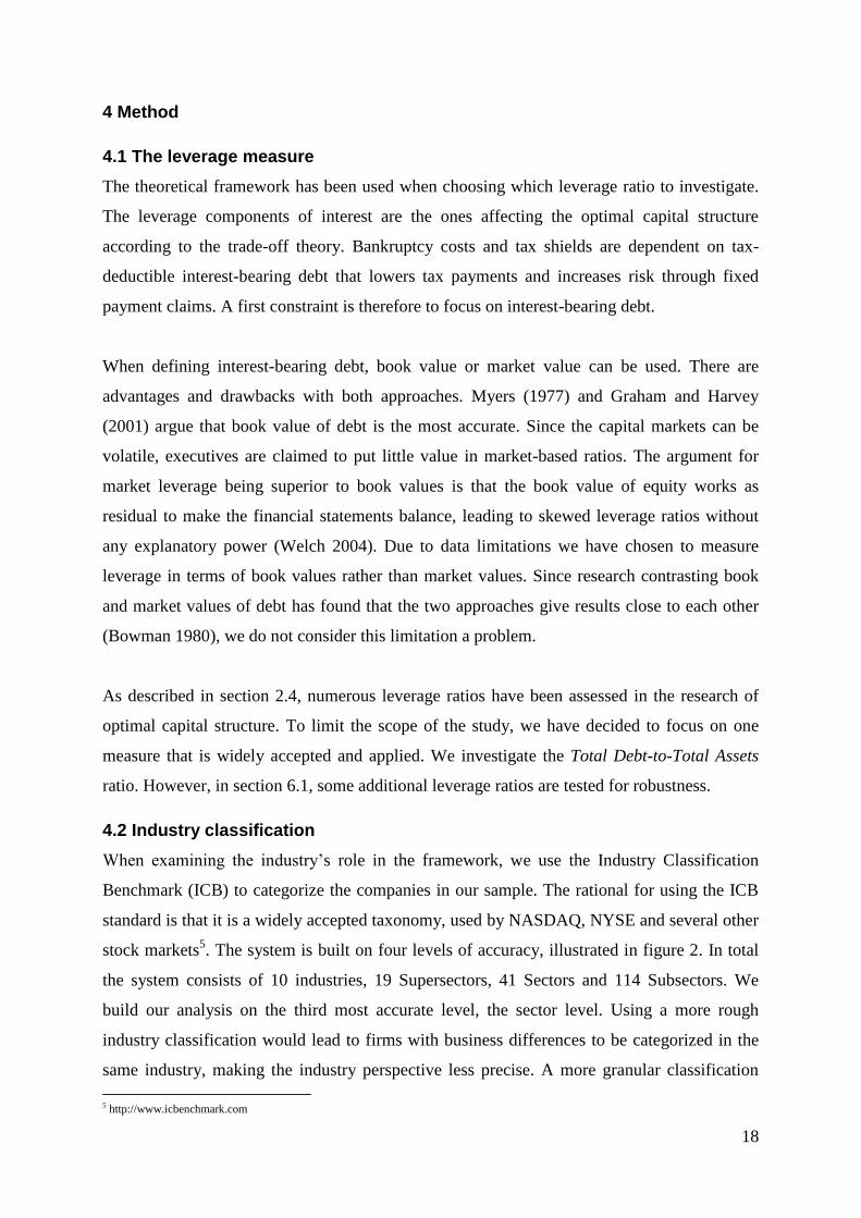
stock markets5. The system is built on four levels of accuracy, illustrated in figure 2. In total
the system consists of 10 industries, 19 Supersectors, 41 Sectors and 114 Subsectors. We
build our analysis on the third most accurate level, the sector level. Using a more rough
industry classification would lead to firms with business differences to be categorized in the
same industry, making the industry perspective less precise. A more granular classification
5 http://www.icbenchmark.com
19
would lead to very few companies in each classification, making it hard to conduct any
analysis on the samples. The yearly mean leverage within each sector is used as industry
standard. When industry standard is mentioned in later sections, we refer to the sector mean.
Figure 2 – Industry Classification (ICB)
4.3 The sample
Since we examine the leverage development over an eleven-year period on the Swedish
market, a panel data set has been compiled for firms listed on the OMX Stockholm stock
Exchange. After screening all listed companies as of year-end 2012, a selection of firms has
been made to fit our analysis. The selection process has been done in the following order.
First, financial institutions have been excluded from the sample. Second, only firms with
available accounting data for all eleven years have been selected. Third, only sectors
consisting of at least 10 companies are included. All steps in the selection process have been
done in line with the methodology used in previous research (Bowen et al. 1982; Byoun 2008;
Lev 1969; Ozkan 2001).
The selections are made with a few objectives in mind. The character of debt in financial
institutions differs from debt in non-financial firms. The financial sector is also regulated,
which affects the leverage ratios. Pure financial firms are therefore excluded from the sample.
By only including firms with complete accounting data for the eleven years we get a balanced
panel of data over the studied time period. Since our analysis to a large extent builds on linear
regressions, see section 4.4.2, missing values would reduce the explanatory power of the
results (Lev 1969; Wooldridge 2013). The criterion of minimum ten firms per sector is made
to make the sector mean leverage ratio more independent of changes in single firms and make
the industry standard robust as proxy for optimal capital structure. The database
DATASTREAM has been used for data collection and STATA 13 has been used for data
handling. By using figures from annual reports we have completed missing values from the
database. In table 3, the sample is presented on sector level. The companies within each sector
Chemicals
Basic Resources
Forestry & Paper
Industrial Metals
Mining
Basic Materials
Paper
Aluminium
Nonferrous Metals
Coal
Forestry
Diamonds
Industry level Supersector level Sector level Subsector level

20
are presented in table 1 in appendix. The firms excluded from the analysis due to data
limitations are presented in table 2, appendix.
Table 3 - Firms in sample
Our sample consists of eight sectors derived from the four wide industry classifications
Industrials, Healthcare, Technology and Financials. To facilitate for the reader in later
sections we use the following sector abbreviations. (1) Construction, (2) Electronic, (3)
Industrial Eng., (4) Support, (5) Healthcare Eq., (6) Pharmaceuticals, (7) Software and (8)
Real Estate.
4.4 Tests
To test the stated hypothesizes and answer the research question several methods are used.
First, variance tests are conducted to answer if the leverage ratio is significantly different
between sectors over time. Second, a partial adjustment model is used to test firms’
movement towards a dynamic target leverage ratio, dependent on a number of firm specific
characteristics. Third, the industry standard as proxy for optimal capital structure is tested
through a partial adjustment model.
4.4.1 Variance test
In accordance with the technique used by Bowen et al. (1982) and Scott and Martin (1975) we
test if the leverage ratio differs across sectors by using a one-way parametric analysis of
variance called ANOVA. The ANOVA test is made for each year on the cross section of
companies in our sample. The idea of the analysis is to test the equality of the mean of a
variable (the leverage ratio) between groups (the sectors) with the null hypothesis that the
mean is the same across the groups. The test is conducted by comparing the within group
variation (SSb) of the chosen variable with the between group variation (SSw) of the variable.
The null hypothesis is tested through an F-test statistic (2) with k-1 numerator degrees of
freedom (k = no. of groups) and n-k denominator degrees of freedom (n = total sample size).
Sector Name Sector Code Industry No. Of firms
(1) Construction & Materials 2350 Industrials 12
(2) Electronic & Electrical Equipment 2730 Industrials 18
(3) Industrial Engineering 2750 Industrials 13
(4) Support Services 2790 Industrials 16
(5) Healthcare Equipment & Services 4530 Healthcare 10
(6) Pharmaceuticals & Biotechnology 4570 Healthcare 13
(7) Software & Computer Services 9530 Technology 21
(8) Real Estate investment & Services 8630 Financials 13

21
Rejection suggests that at least one of the means is different from the others (Newbold,
Carlson & Thorne 2010).
(2)
⁄
⁄
The ANOVA-test is a parametric test, which assumes that the population from which the
sample is obtained is at least approximately normally distributed. If this assumption is
violated, the test may return biased results. Also, the test statistic can be rendered by large
inequalities in sample sizes. To avoid the risk of drawing conclusions on biased results, we
also conduct the non-parametric Kruskal-Wallis one-way analysis of variance. The null
hypothesis is stated in accordance with the ANOVA-test, with the difference that the Kruskal-
Wallis test investigates median values. The test statistic stated in (3) is calculated by
organizing the observations (the leverage ratios) by rank.
(3)
(∑
)
T and n is the rank sum and sum of firms in the sectors. is the number of firms in each
sector. Under the null hypothesis, since all our sectors consist of more than six firms, the
distribution of H will approximately follow a χ2 distribution with (k-1) degrees of freedom.
Rejection of the null hypothesis suggests that at least one of the sector medians is different
from the others (Newbold, Carlson & Thorne 2010). We use a 10% significance level to
define the rejection region.
If both tests lead to rejection of the null hypothesis, post-hoc multiple comparisons are
conducted to see which sectors that are significantly different from each other in each year.
The sectors are pairwise tested for different average values. Since we are comparing several
sectors simultaneously, a multiple comparison problem occurs, leading to an increased
family-wise error rate. This means the rate of type 1 errors will escalate by each comparison,
increasing the risk of one or more false rejections of the null hypothesis. We handle this
problem using a Bonferroni adjustment, dividing the critical alpha value by the number of
pairwise tests to keep the family wise error at a constant level (Leon, Heo 2005).

22
4.4.2 Partial adjustment model
The second hypothesis, , is tested through a partial adjustment model. The partial
adjustment model we use builds on the same model first created by Lev (1969), further
developed by Ozkan (2001) and Flannery and Rangan (2006). The idea of the model is to
measure the speed by which a firm’s leverage ratio is adjusted towards a target. As stated in
section 4.1, the leverage ratio we test is the interest bearing debt ( ) to total assets ( ).
We compute the ratio for every firm, i, in each year, t, over the eleven-year period, in
accordance with equation 4.
(4)
There are numerous ways of estimating the target leverage ratio. Byoun (2008), Flannery and
Rangan (2006) and Ozkan (2001) estimate the target based on yearly cross sectional
regressions of the observed ratio on firm characteristics said to determine capital structure.
This method builds on the assumption that the observed debt ratio in each time period is the
optimal level and that the adjustment towards the target is perfect each year (Byoun 2008).
Another approach is to assume the industry average of leverage to be the optimal level in each
time period. We use both the firm characteristics ( ) and industry standard ( ) approach, as
described by step 1 and 2 in figure 1, section 3. However, in the earlier, due to lack of
observations, we use panel data over eleven years and a fixed effect regression6. The
interpretation is the same as the one from a cross sectional regression and since we estimate
using observed debt ratios, the perfect adjustment assumption stands intact (Flannery,
Rangan 2006). The estimation of a target using firm characteristics is illustrated in equation 5.
The target ratio is estimated through a regression of the leverage ratio on a number of firm
characteristics, , empirically found to be leverage determining.
(5)
∑
The perfect adjustment assumption in equation 5 does not allow for a partial adjustment
towards the target over time. However, in the presence of adjustment costs and other
imperfections, the assumption of immediate convergence needs to be relaxed. It is rather more
6A methodology also applied by Antoniou et al. (2008). Argued to provide more robust target estimations than the cross sectional approach
since the regression can be done with firm and year fixed effects (method described in section 4.4.2.3).

23
interesting to find if there is any partial adjustment towards the target over time or not. By
plugging in the fitted value from equation 5 in the partial adjustment model specified in
equation 6 and 7, the perfect adjustment assumption is relaxed and the gradual movement
towards a target can be measured (Byoun 2008; Flannery, Rangan 2006; Ozkan 2001).
(6) ( )
(7)
( ) or is interpreted as the “target change” a firm should make to reach the
optimum. or is the actual change of leverage and the fraction of target
change achieved over the measured period. If takes the value 1, there is a perfect adjustment
towards the optimum. Without any refinancing costs, the adjustment would be perfect, as
assumed in the static trade-off theory and predicted in the estimation of . However, in the
presence of refinancing costs, the adjustment is harder to predict. The partial adjustment
model assumes that the cost of adjustment towards a target is independent of the target
leverage change and provides an indication of how substantial the refinancing costs are
(Flannery, Rangan 2006).
4.4.2.1 Firm characteristics as determinants of L*
We estimate by inserting firm specific variables ( ) in equation 5, empirically recognized
as capital structure determinants. In total we use six explanatory variables that are most
frequently applied by previous research. Below, each variable is described. The variables’
predicted effects within the trade-off framework are summarized in table 4.
Profitability – In accordance with previous research, we use the EBIT-margin, defined as
operating profit divided by sales, to measure a firm’s profitability (Fama, French 2002;
Flannery, Rangan 2006). We find this ratio a suitable proxy since operating profit is the result
used to benefit from an interest tax shield provided by debt. As stated in the theoretical
framework, profitability should over time have a positive relationship with leverage due to the
tax shield advantage. However, the dynamic setting may dampen the positive effect.
Earnings volatility - We estimate earnings volatility with the yearly standard deviation of
quarterly earnings. Since increased volatility is associated with higher bankruptcy risk, a

24
relationship described in the theoretical framework, the trade-off framework predicts a
negative leverage effect from the variable.
Size – The log of total assets is used to proxy firm size. This proxy has been applied and
verified in several previous studies (Frank, Goyal 2009; Titman, Wessels 1988). According to
the framework presented in section 2.3.1, size is predicted to have a positive effect on
leverage.
Tangibility of assets – We approximate tangibility of assets by each firm’s Fixed Asset-to-
Total Asset ratio. This method is also in line with previous research (Byoun 2008; Flannery,
Rangan 2006; Frank, Goyal 2009). As stated in the theoretical framework, tangibility of assets
should be positively correlated to firms’ leverage ratios.
Depreciation – The non-debt tax shield provided by depreciation is measured by
depreciation as fraction of total assets. This proxy is also applied in previous research (Ozkan
2001; Titman, Wessels 1988). According to the theoretical framework in section 2.3.1, the
non-debt tax shield substitutes the leverage benefits of debt. This should lead to a negative
relationship between the independent variable and the leverage ratio.
Growth – Previous studies, using market values to measure the investigated leverage
ratios, normally apply firms’ market value to book ratio as proxy for predicted growth (Byoun
2008; Fama, French 2002; Flannery, Rangan 2006; Ozkan 2001). Since we are taking an
internal perspective, measuring leverage ratios using book values, we find the market to book
ratio unsuitable as proxy. Instead, we take a retrospective approach and use each firm’s yearly
change in log assets to measure growth. This proxy is also empirically found to be capital
structure determining (Frank, Goyal 2009). In the robustness section, we also test growth in
sales as determinant for leverage. As discussed in section 2.3.1, growth is expected to have
negative effect on the leverage ratio.
Table 4 –Predicted signs of coefficients
Coefficient Xk Predicted Sign
β1 Profitability +
β2 Earnings volatility -
β3 Size +
β4 Tangibility of Assets +
β5 Depreciation -
β6 Growth -

25
4.4.2.2 Industry standard ( ) as proxy for optimal leverage
Inspired by Lev (1969) and Flannery and Rangan (2006), in step 2 of the analysis (Illustrated
in figure 1, section 3), the partial adjustment model is used to test the industry average ( ) as
proxy for optimal leverage. This proxy builds on the assumption that the trade-off between
debt and assets is similar within industries and different across industries (Flannery, Rangan
2006), an assumption first scrutinized through tests of the hypothesis . The industry
standard used is the mean leverage value on sector level, leading to the modified partial
adjustment model described by equation 8 below.
(8) ( )
In equation 8, is the sector average leverage ratio in time t. In this setting, the speed of
adjustment, , is towards the common leverage level within each sector.
4.4.2.3 Fixed effects and sector dummy variables
In the estimation of target leverage using firm characteristics, a fixed effects model is used to
handle unobservable variables that can lead to biased results in the regression. This means
each variable described in section 4.4.2.1 is differenced over time to filter the results from
firm specific factors that are constant over time but different among firms and not included
among the explanatory variables. Year dummy variables are also included in the regression of
L* in equation 5 to filter the results for time specific factors affecting all firms’ optimal
leverage. Examples of filtered effects are tax rate changes and general business cycles.
Running the regression without these adjustments would increase the risk of creating an
underspecified model returning results biased by omitted variables (Wooldridge 2013).
Previous research has also stressed the risk of autocorrelation (correlation between over
time) and heteroskedasticity (changing variance in over time) when estimating the stated
regressions in section 4.4.2 (Fama, French 2002; Lev, 1969; Ozkan, 2001). In accordance
with Ozkan (2001), we assume the error term to be serially uncorrelated and use robust
standard errors to handle potential heteroskedasticity when running regression 5, 6, 7 and 8.
This method is aimed to reduce the risk of biased firm characteristic- and speed coefficients.
The industry perspective, which is a focal point in the thesis, is based on a comparing
approach. By interacting the adjustment coefficient in equation 6, 7 and 8 with eight sector

26
dummy variables, the speed of adjustment is contrasted between the investigated sectors. The
adjustment speed within one of the sectors is used as base case and then compared to the
speeds of the other sectors by two-tailed t-tests. For each sector, the null hypothesis ,
that the speed is not different from the base-case, is tested with the two-sided alternative
hypothesis , that the speed differs from the base case. Through this procedure, we
investigate if sector belonging affects the results from tests of the stated null hypothesis in
section 3.
4.5 Method critique
Several studies highlight the drawbacks of the partial adjustment model building on fixed
effect estimations (Nickell 1981; Ozkan, 2001). Since the target adjustment speed may be
correlated with the error term in equation 6, 7 and 8, the found adjustment speed could be
biased. It is also argued that the relationship between the dependent and explanatory variables
in the model is non-linear which makes the linear regression method described above an
inappropriate technique (Ozkan 2001). The highlighted problems with the regression method
have been handled through a number of advanced econometric approaches such as lagged
instrumental variables (Dang 2013; Ozkan 2001). However, no method is proved superior to
the basic approach (Huang, Song 2009). Therefore, the method described in section 4.4.2 is
kept but the interpretation of the results is made with the limitation of the model in mind.
More advanced frameworks consider the described partial adjustment model too simplified in
explaining the adjustment speed. Dang (2013) argues the assumption of independence
between refinancing costs and target change to be unrealistic when developing a more
sophisticated error correction model. Also, the applied fixed effects model when estimating
the target leverage, L*, in equation 5 may lead to exaggerated significance levels due to the
large number of observations (Wooldridge 2011). The simplified assumption and chosen
method stated in section 4.4.2 constrains the interpretation of reached results.
The consequences of using a method with variables measured by book values must also be
commented upon. By taking an internal perspective of the analysis and focusing on book
values of the leverage ratio, the firms’ adjustment in response to external chocks is neglected.
This limits the interpretation of the achieved results from the study. Nothing can be said about
how firms behave in relation to dynamics in the capital markets or macro-economic chocks.

27
Also, the estimated leverage for each firm ignores measurement errors derived from
accounting methods. This may lead to inaccuracies when mapping the leverage development
to answer the null hypothesis . For example, firms in R&D heavy sectors such as Software
and Pharmaceuticals recognize intangible assets in accordance with the International
Accounting Standard 38 (IAS 38). Since each firm makes an assessment of internally
developed intangibles, firms with similar projects and businesses might generate different
ratios of capitalization. Increasing investments in combination with capitalization leads to a
higher solidity (White, Sondhi & Fried 2003), which may lead to subjective evaluations and
biased leverage ratios. Enea, Novotek and Addnode are firms included in our analysis
exposed to this potential measurement error. A required assumption is therefore that the firms
in our sample have similar strictness when assessing internally developed intangible assets.
Treatment of lease contracts is another example of how accounting methods may lead to
misleading leverage measures, affecting comparability between firms. In accordance with IAS
17, a lease agreement can either be considered financial or operating. A finance lease will
give rise to a debt-financed asset on the firm’s balance sheet and a higher leverage ratio. An
operating lease agreement will not give rise to a debt-financed asset (White et al. 2003).
Several companies in our sample have both financial lease- and operating lease agreements. A
necessary assumption is therefore that all firms make the right classification and show truthful
leverage ratios in their books.
Lastly, the selection process described in section 4.3 is supposed to facilitate the analysis.
However, the data collection also leads to certain shortcomings that may restrict us in our
conclusions. A consequence of only including firms with complete accounting data for the
eleven years is that only firms that have survived during the period are included. The
survivorship bias means we need to be cautious when drawing general conclusions from the
analysis. Also, a logic consequence from the Swedish focus of our analysis is that our results
will not necessarily be applicable on other markets. All the above stated risks and
shortcomings should be considered when interpreting our results.

28
5 Results and analysis
In the following section, we present the results and analysis in three steps. First, the leverage
development at sector level is investigated in section 5.1. Second, results from the partial
adjustment model are presented with firm characteristics as determinants of optimal leverage
( ) (Step 1 in figure 1). Third, results from the tests with an industry standard ( ) as proxy
for optimal leverage are presented (Step 2 in figure 1).
5.1 Leverage development on the Swedish market (Test of )
Figure 3 illustrates the mean leverage development among the selected sectors on the Swedish
stock market between year 2002 and 2012. The graph shows that Real Estate consistently has
been the highest leveraged sector and Software the lowest. These first findings are in line with
the theory presented in section 2.3.2 and with previous research presented in section 2.4.2.
Software together with Pharmaceuticals are sectors known to be dependent on high R&D
costs and thus associated with higher operating risk than for example the Construction and
Real Estate sectors. Industrial Eng., Construction and Electronic are quite similar sectors
where firms have considerable proportions of property, plant and equipment on their balance
sheets. These sectors all show higher mean leverage than the Software and Pharmaceuticals
sectors over the time period.
Figure 3 - Mean leverage development (Debt / Total Assets), 2002-2012
The results from the ANOVA and Kruskal-Wallis tests are presented in table 5 to verify the
sector differences in leverage that seem to prevail. As seen in the table, at least one of the
sector means and medians is significantly different from the others in each year. The
parametric ANOVA test returns high F-values leading to a rejection of the null hypothesis,
that all means are equal, at a 1% significance level in every year. The Kruskal-Wallis test
shows the same significant results with persistently high chi-square values.
0%
10%
20%
30%
40%
50%
60%
2002 2003 2004 2005 2006 2007 2008 2009 2010 2011 2012
Construction
Electronic
Industrial Eng.
Support
Healthcare Eq.
Pharmaceuticals
Real Estate
Software

29
Table 5 – ANOVA (F) & Kruskal-Wallis (χ²) test of leverage differences
After rejecting the null hypothesis of the initial ANOVA and Kruskal-Wallis tests, post-hoc
comparisons have been conducted to find which of the sectors that significantly differ from
each other over time. Table 6 shows a summary of the results from the post-hoc comparisons.
All sectors are compared to each other in each year. In each row, the upper figure shows the
average leverage difference (percentage points) between each pair of sectors over the eleven
years. The lower figures show number of years with significant differences (Rejection at a
10% significance level). Figures not in parenthesis indicate number of years with significant
results according to the ANOVA post-hoc comparisons (mean leverage values). Figures
within parenthesis indicate number of years with significant differences according to the
Kruskal-Wallis post-hoc comparisons (median leverage values). The Bonferroni adjustment is
applied in both tests. All yearly tests are presented in table 3 and 4, appendix.
Table 6 - Pairwise ANOVA & (Kruskal-Wallis) post hoc comparisons
The pairwise comparisons give insight into which sectors that differ from each other over
time. In a majority of the years, mean and median leverage is significantly different in the
Real Estate sector compared all other sectors. Both the ANOVA and Kruskal-Wallis post-hoc
comparisons confirm persistently higher leverage within the sector. This is a predicted
outcome since the sector has had a remarkably high mean leverage compared to all other
sectors over the years. Software has significantly lower leverage than all sectors but
Healthcare Eq. and Pharmaceuticals in a majority of the years. This further verifies the
reasoning in section 2.3.2 regarding R&D intensive businesses. However, sectors within the
Construction Electronic Healthcare Eq. Industrial Eng. Pharmaceuticals Real Estate Software
Eletronic5%
0 (0)
% Diff
ANOVA (KW)
Healtcare Eq.8%
0 (0)
4%
0 (0)
Industrial Eng.4%
0 (0)
5%
0 (0)
8%
0 (0)
Pharmaceuticals14%
2 (0)
9%
0 (0)
5%
0 (0)
14%
2 (3)
Real Estate22%
9 (6)
27%
11 (9)
30%
10 (7)
22%
9 (6)
36%
11 (10)
Software19%
8 (11)
14%
2 (7)
11%
0 (0)
19%
9 (10)
5%
0 (0)
44%
11 (11)
Support4%
0 (0)
2%
0 (0)
4%
0 (0)
5%
0 (0)
9%
0 (0)
27%
11 (9)
13%
6 (6)
Year 2002 2003 2004 2005 2006 2007 2008 2009 2010 2011 2012
F 12,43***
11,39***
9,91***
6,19***
5,41***
7,60***
7,53***
9,47***
10,02***
12,75***
10,57***
χ239,06
***37,28
***34,45
***34,27
***34,08
***34,64
***36,25
***35,80
***37,56
***41,73
***40,8
***
***p<0,01 **p<0,05 *p<0,1

30
same general industry do not have significantly different leverage from each other in any time
period. This can be seen in the pairwise comparisons between the four sectors Electronic,
Construction, Industrial Eng. and Support, all sectors derived from the general industry
Industrials. The results indicate that firms within the same general industry have enough
common capital structure characteristics to be regarded similar in each year.
Over all, the results from the variance analysis lead to a rejection of the null hypothesis
when following the rejection rule stated in section 3. There seem to be inter-industry
differences in leverage over the years. However, since the sectors within a common industry
show similarities, one could argue that a more rough industry classification is enough to
contrast different types of businesses in the trade-off framework. A rougher industry
classification would also be more in line with some of the previous research that has verified
inter-industry differences (Schwartz, Aronson 1968; Scott, Martin 1975). However, the
granular classification might still add to the further analysis by contrasting sectors that appear
similar. We therefore keep the more accurate perspective.
5.2 The partial adjustment model (Test of )
The result from the partial adjustment model is reported in two steps, as described in figure 1,
section 3. First, firms’ adjustment speeds towards the estimated target L*, as described in
section 4.4.2, are presented and contrasted between sectors. Since the sector comparison in
section 5.1 led to rejection of , the second step of the analysis is thereafter conducted by
measuring the adjustment speed towards the industry standard, , defined as sector mean
leverage in each year.
5.2.1 Firm characteristic determinants
Before using the fitted values from regression 5 (section 4.4.2) in the partial adjustment
model, the outcome of the regression is examined to give an initial picture of how firm
characteristics affect the leverage target. The regression results are presented in table 7
together with the predicted signs from the trade-off theory. All regressions can be found in
table 5 and 6, appendix. The regression is first made on the whole sample and thereafter on
sector level. The sector level regressions are made to investigate whether the inter-sector
perspective plays an important role in the analysis or not. If the sector level regressions all
show homogenous results in line with the whole sample regression, the explanatory variables
would not be dependent on sector belonging. Then an inter-industry perspective again could
be argued irrelevant for the analysis even though the null hypothesis has been rejected.

31
Table 7 – Determinants of L*
We find that in the regression on the whole sample, a majority of the variables show signs in
line with the outcomes predicted by the trade-off theory. Size, profitability, volatility and
tangibility of assets all show significant values in line with the predicted outcome in the trade-
off theory, even though the coefficients for profitability and volatility are small. Depreciation
is the only variable showing an unexpected leverage effect. The explanatory power of the
regression is high, indicated by an R2
value of 0.48.
The regressions made on sector level show less unanimous results. Size and tangibility are the
only coefficients with signs matching the predicted outcome in all the investigated sectors.
Volatility does not have significant impact on leverage within any of the sectors. Either
volatility is not a capital structure determinant as previous research has found, or our
specification of the proxy described in 4.4.2.1 fails to capture the leverage affecting risk
associated with increased volatility. The proxy used for profitability and growth show
scattered results without any clear interpretation in line with the trade-off theory. Healthcare
Eq., Pharmaceuticals, Real Estate and Support are the only sectors where a majority of more
than one significant variable are in line with the prediction from the trade-off theory. For the
Healthcare Eq. sector, all signs are in line with theory and many of the coefficients are
significant below a 10% level. Industrial Eng., Construction and Software are sectors on the
other side of the spectra, showing the opposite sign to the predicted for many of the
significant variables.
Obviously, firm characteristics have different effects on leverage within different sectors.
This result is in line with the rejection of hypothesis in section 3. Different sectors do not
only seem to have persistently different leverage ratios, firm characteristics are also affecting
the leverage ratio differently between sectors.
Growth Size Profitability Depreciation Volatility Tangibility No. of obs. R2
Predicted outcome - + + - - +
1 Whole sample -0.003 0.048 *** 0.004 *** 0.012 -0.0009 * 0.237 *** 1160 0.480
By Sector
2 Construction 0.092 0.074 ** -0.881 *** 1.787 ** -0.002 0.405 *** 120 0.204
3 Electronic -0.010 0.067 *** 0.003 0.236 -0.001 0.073 180 0.162
4 Industrial Eng. 0.026 ** 0.024 -0.002 1.158 *** 0.001 0.075 130 0.354
5 Support 0.010 0.027 * -0.401 *** -0.924 * -0.004 0.353 *** 160 0.555
6 Healthcare Eq. -0.079 ** 0.014 0.047 * -0.527 * -0.001 0.290 *** 100 0.324
7 Pharmaceuticals -0.001 0.025 ** 0.004 *** 0.111 -0.001 0.157 *** 130 0.287
8 Real Estate 0.001 0.022 -0.005 -0.647 *** -0.001 0.505 *** 130 0.535
9 Software 0.004 0.040 *** -0.044 * 0.238 *** -0.003 0.175 *** 210 0.200
***p<0,01 **p<0,05 *p<0,10

32
5.2.2 Speed of adjustment (Step 1)
Since the sector specific regressions show results widely different from each other, each
industry specific estimation of L* (row 2-9 in table 7) is used in the partial adjustment model
when comparing the speed of adjustment between industries. Using the regression on the
whole sample (row 1 in table 7) also when comparing the industries would lead to estimated
debt ratios influenced by companies from all different sectors. With big sector differences,
this alternative approach would clearly lead to an imprecise analysis.
The results from the partial adjustment model are presented in table 8. The speed of
adjustment is first measured for the whole sample towards the target estimated in row 1 in
table 7 to find out if there is any general adjustment in line with the trade-off theory. After the
initial speed measurement, the different sectors are contrasted to find if the adjustment speed
differs between the sectors. The sector comparison is conducted by interacting all sectors with
the adjustment coefficient and using Healthcare Eq. as base case.
Table 8 – Speed of adjustment towards L*
For the whole sample, there is a significant adjustment speed of 0.164 towards L*,
demonstrating that companies adjust towards a target, in accordance with the trade-off theory.
In the sector comparison, a majority of the sectors show the same adjustment speed, not
significantly different from the speed within the base case sector. However, within the
Pharmaceuticals sector, the movement towards a target seems to be non-existing. This result
stands in contrast to the outcome described in section 5.2.1. When estimating L* in table 7,
Pharmaceuticals was one of the sectors that best followed the predicted outcome. Even
though the explanatory variables affect the debt ratio in accordance with the trade-off theory,
Coefficient Std. Err. t-value No. Of obs. R2
Adjustment, whole sample (δ) 0.164 0.014 11.60***
1160 0.104
Sector comparison (δ) 0.188 0.049 3.83***
1160 0.100
Construction -0.092 0.064 -1.43
Electronic -0.025 0.055 -0.45
Industrial Eng. 0.037 0.067 0.56
Support -0.033 0.062 -0.54
Pharmaceuticals -0.189 0.049 -3.84***
Healthcare Eq. 0 (omitted)
Real Estate -0.050 0.052 -0.95
Software -0.042 0.075 -0.56
***p<0,01 **p<0,05 *p<0,10

33
no adjustment towards the estimated target can be found. Conditional on correctly specified
firm characteristics, the dynamic model captures important inter-sector differences in
adjustment speed. While the model captures an adjustment speed for a majority of the sectors,
it fails to explain the leverage development within the Pharmaceuticals sector. Firms within
this sector are obviously not following the theoretical framework presented in section 2 to the
same extent as firms in the other sectors are. The initial estimation of L* in line with the trade-
off theory gives the impression that firms within the Pharmaceuticals sector actually are
weighting the benefits from debt with the costs associated with higher leverage. However, the
non-existing speed of adjustment indicates that deviation from the target is ignored.
Following the rejection rule stated in section 3, the results from the target estimation and
partial adjustment model lead to a general rejection of the null hypothesis in step 1 of the
analysis. In the regressions made on the whole sample, a majority of the chosen firm
characteristics affect the target in accordance with the trade-off theory and the adjustment
towards the target is significant. A significant adjustment speed is also found within a
majority of the sectors. However the Pharmaceuticals sector shows contrasting results. Also,
since many of the coefficients on sector level in table 7 show signs contradicting the
prediction in the trade-off framework, the adjustments on sector level cannot in isolation be
interpreted as results explained by the theory. Even though firms in a majority of the sectors
seem to weight pros and cons of leverage and adjust towards an optimal trade-off between the
factors, the optimal point is not fully explained by the theoretical framework.
5.2.3 Industry standard ( ) as proxy for optimal leverage (Step 2)
Backed by the rejection of , the trade-off theory is also tested with the sector standard ( )
as proxy for optimal leverage. The results are presented in table 9 below, showing the
outcome both for the whole sample and the sector comparison. To clarify, the whole sample
regression is made without including sector interaction dummies but still with sector specific
leverage targets. In this setup, the sector comparison is conducted by using Software as base
case.

34
Table 9 – Speed of adjustment towards
The outcome from the modified partial adjustment model shows results overall in line with
the model using firm characteristics as target determinants. The adjustment speed for the
whole sample is 0.136 and significant at a 1% level. The inter-sector comparison shows a
homogenous speed of adjustment independent from sector belonging. No sector shows a
speed of adjustment significantly different from the base case sector Software. The conflicting
result from the Pharmaceuticals sector in the previous section is not apparent when using the
sector average as proxy for optimal leverage. Firms within all sectors show significant
positive adjustment speeds toward the sector average. The industry standard seems to be an
appropriate proxy for optimal capital structure. The results are comparable with a target
estimated by firm characteristics. Over time, firms within all sectors converge towards the
sector mean leverage value.
The analysis of firms’ adjustment towards a target leverage ratio in step 2 of the analysis leads
to an additional rejection of the null hypothesis . Firms do not only seem to follow a firm
specific target when adjusting their leverage ratio in accordance with the trade-off theory, the
industry standard also seems to play a role in the framework.
6 Discussion
There are several aspects of the method applied that may have affected the results stated in the
previous section and thus need to be commented upon. Also, the interpretation limitations of
the achieved results are obvious when allowing for a wider analytical perspective. Below, a
critical discussion of the method, results and analysis follows.
Coefficient Std. Err. t-value No. Of obs. R2
Adjustment, whole sample (δ) 0.136 0.013 10.05***
1160 0.080
Sector comparison (δ) 0.147 0.059 2.46**
1160 0.085
Construction -0.026 0.075 -0.35
Electronic 0.016 0.067 0.23
Industrial Eng. -0.008 0.074 -0.11
Support -0.062 0.069 -0.90
Healthcare Eq. -0.064 0.072 -0.88
Pharmaceuticals -0.005 0.077 -0.06
Real Estate 0.024 0.066 0.36
Software 0 (omitted)
***p<0,01 **p<0,05 *p<0,10

35
Examining the null hypothesis with an ANOVA-test assumes normal distribution of the
underlying population. We have not been able to verify that the population is normally
distributed through skewness and kurtosis tests of normality on our sample. Also, the
compared samples are of different sizes, which make the ANOVA-test less powerful. With
these shortcomings in mind, conclusions from the test need to be drawn with caution.
However, since the non-parametric Kruskal-Wallis test generated results in line with the
parametric test, the null hypothesis can be rejected with additional certainty. Our results are
well in accordance with previous research, indicating that there are persistent inter-industry
differences and intra-industry similarities in leverage. Yet, the granular sector classification
leads to insignificant differences among sectors within the same general industry. Therefore
our evidence for industry differences is weaker than the proof provided by Bowen et al.
(1982) who found differences between firms in granular sectors within common industry.
In light of the results in section 5.2.1, we find it important to further discuss the double-faced
nature of firm characteristics, previously addressed in section 2.3.1. Even though this study
focuses on testing the trade-off theory, a total isolation from other perspectives would limit
the interpretation of the results and lead to several uncommented question marks. The
regression of L* made on the whole sample, presented in table 7, indicates that the trade-off
theory can explain most firm characteristic leverage effects. However, the sector wise
regressions show scattered results. We interpret the results in accordance with the previous
studies presented in section 2.4.1. Full understanding of how firm specific characteristics
affect the capital structure target cannot be accomplished through a single theory perspective.
It seems like different theories co-exist and work as complements rather than substitutes in
explaining firms leverage ratios on the Swedish stock market. For example, within both the
Construction and Support sector, a significant negative relationship is found between
profitability and leverage. The outcome is in line with all the presented previous findings but,
as stated by Frank and Goyal (2009), better explained by the pecking order theory. Also, the
positive leverage effect of depreciation found in the Construction and Industrial Eng. sectors
stands in contrast to the predicted effect and previous findings. Referring to the reasoning by
Bradley et al. (1983), we conclude that firms in these sectors may follow the secured debt
theory, rather than using depreciation as tax shield when determining debt levels.
The scattered findings limit the rejection of the stated null hypothesis . The theory does not
provide a comprehensive explanation of the target on sector level, indicating that other

36
frameworks sometimes may better explain firms’ leverage ratios. The trade-off theory stands
out as a good explanatory framework within the Healthcare Eq., Real Estate and Support
sectors. Within these sectors, a majority of several significant variables affect leverage as
predicted and the adjustment speeds are significant. The other sectors show ambiguous results
when estimating the target leverage ratio on firm characteristics.
When applying the partial adjustment model to investigate the null hypothesis , we find
homogenous significant adjustment speeds towards both alternative leverage targets in a
majority of the sectors (step 1 & step 2). However, the fast adjustment towards a target based
on firm characteristics, identified in some of the previous research, is not apparent in our
study. The slow adjustment speeds are in accordance with the findings by Fama and French
(2002) and may be explained by substantial refinancing costs associated with leverage
correction. The risk of exaggerated speed coefficients caused by omitted variables is handled
through a fixed effects model with year dummies. However, due to the flaws of the model
described in section 4.5, rejection of the null hypothesis is done with caution. The
survivorship bias and geographical limitation of our study, described in section 4.3 also
restrains the rejection of on a general basis.
The model based on firm characteristics applied in the first step of the analysis fails to explain
the leverage development within the Pharmaceuticals sector. Since the adjustment towards a
sector average exists for the Pharmaceuticals sector, the partial adjustment model based on
firm characteristics could be argued to suffer from under-specification. There may be
important capital structure determinants missed out in the model described in section 4.4.2.1,
later caught by the proxy in step 2 of the analysis. The potential under-specification is further
investigated in section 6.1.
6.1 Robustness
With the critical discussion regarding shortcomings of the method and limitations of the
interpretations in mind, a number of adjustments have been made to test the robustness of the
findings in section 5 and the rejection of the null hypothesizes.
First, the risk of omitted variables affecting the results has led to a further investigation of
possible capital structure determinants. As previous research highlights in section 2.4.1, R&D
can affect leverage in technology-dependent sectors. Therefore, a re-run of regression 5, 6 and

37
7 has been made, including R&D as fraction of sales as an additional explanatory variable.
This robustness check did not provide any better understanding of the leverage development.
The fraction of R&D had no significant impact on leverage and the speed of adjustment was
still missing within the Pharmaceuticals sector. As an alternative to the change in log assets,
we have also included yearly sales growth in equation 5 as proxy for growth. The effect from
the sales growth is consistent with the growth proxy used in section 5, adding no further
explanatory power to the model.
To add further reliability to the rejection of the null hypothesis , we investigate if
adjustment speeds depend on firm size. Companies within each sector have been divided into
sub-samples of small, mid- and large-cap firms, as defined by NASDAQ OMX Nordic7.
Thereafter, the speed of adjustment has been measured for each group within the sectors. The
same method used to contrast the different sectors is applied in the size comparisons
(described in section 4.4.2.3). A summary of the results is presented in table 10. All
comparing regressions can be found in table 7, appendix. Since the already small sized sector
samples are divided into even more granular subsamples, some of the groups consist of a
small numbers of observations, making the regression method less appropriate. Regressions
on sub-samples with the least observations therefore need to be interpreted with caution.
Table 10 - Speed of adjustment, size comparison
The comparison shows important differences between the size groups. Even though there
seems to be significant movement within a majority of the sectors and size groups, firms in
the large and mid-cap groups show faster and more significant speeds of adjustment than
firms in the small-cap group. Also, when comparing the speed coefficients between the
7 http://www.nasdaqomxnordic.com/aktier
ADJ Coefficient (δ) Large Cap ( ) Mid Cap ( ) Small Cap ( ) Large Cap ( ) Mid Cap ( ) Small Cap ( )
Construction 0.106 * 0.231 *** -0.056 0.116 * 0.209 *** -0.037
Electronic 0.901 *** 0.249 *** 0.173 *** 0.907 ** 0.217 *** 0.164 ***
Industry Eng. 0.251 *** 0.368 *** 0.161 0.251 *** 0.232 ** 0.069
Support 0.354 * 0.126 * 0.221 *** 0.354 * 0.112 * 0.090 ***
Healthcare Eq. 0.477 *** 0.544 ** 0.114 ** 0.477 *** 0.601 *** 0.098 *
Pharmceuticals 0.146 0.000 -0.003 0.146 0.094 0.276
Real Estate 0.146 *** 0.229 *** - 0.145 *** 0.239 *** -
Software 0.476 ** 0.295 ** 0.124 *** 0.476 ** 0.173 * 0.137 ***
No. Of observations Large Cap Mid Cap Small Cap
Construction 50 50 20
Electronic 10 60 110
Industry Eng. 80 30 20
Support 10 40 110
Healthcare Eq. 20 20 60
Pharmceuticals 30 40 60
Real Estate 60 70 -
Software 10 20 180
***p<0,01 **p<0,05 *p<0,10
L* L* L* L L L

38
groups, the speed of adjustment is persistently lower and often insignificant for the small-cap
firms (See table 7, appendix). Rejection of must therefore be restricted to large- and mid-
cap firms. The results contrast the conclusion reached by Flannery and Rangan (2006) who
found the opposite relationship between size and adjustment speed. Small firms having high-
risk profiles and low bargaining power, leading to high refinancing costs, may explain the
neglected targets8.
Since single companies with extreme values might skew the sector mean proxy, the
adjustment regression (equation 8) has been recalculated with sector median leverage as
proxy for an optimal level (Not presented in appendix). The found adjustment speeds towards
a median are consistent with the results presented in section 5.2.3. All sectors show the same
significant adjustment speed towards the target, in line with the trade-off theory. The
homogenous results from mean and median targets contribute with additional robustness to an
industry standard as proxy for optimal leverage level.
The target leverage ratio used in step 2 of the analysis in section 5 is derived from accounting
figures presented at the end of each time period. Arguably, a more realistic assumption is that
firms adjust towards a target based on accounting figures from the latest period known.
Therefore, the target in equation 8 has been replaced with a one year lagged variable of
leverage ( ). The re-run of the regressions shows no different results from the initial
analysis, which means the proxy stands robust. However, with the steady sector mean
leverage ratios in mind (illustrated in figure 3), the similar outcome from a lagged variable is
expected.
The analysis presented in section 5 is focused on how firms adjust the single leverage ratio
book value of Total Debt-to-Total Assets in relation to an estimated target. To add further
robustness to the discovered adjustment speeds, the speed coefficient is measured for the two
alternative leverage ratios Long Term Debt-to-Total Assets (LTD/TA) and Common Equity-
to-Assets (E/A). These ratios are also used in the presented previous research. The use of
alternative leverage ratios as dependent variables provide further proof in line with rejection
of the null hypothesis . As can be seen in table 11 below, a majority of the sectors show
significant adjustment speeds independent of which leverage ratio and target type used in the
8 An argument in line with the reasoning by Titman and Wessels (1988)

39
analysis. The non-adjustment within Pharmaceuticals is also persistent, showing insignificant
adjustment for all ratios based on firm characteristics.
Table 11 – Speed of adjustment with different leverage ratios
The adjusted models and added perspectives lead to both additional robustness and need for
further isolation of the achieved results in section 5. While the size comparison indicates
insignificant adjustments within small-cap firms, the multiple leverage ratio perspective adds
further evidence in line with the rejection of . In addition, the industry standard stands out
as a good proxy for optimal capital structure after the further investigation.
6.2 Reliability, validity & generalizability
In the light of the methods used and results found, our study’s validity, reliability and
generalizability should be commented upon. The methods used in the study follow previous
practice to a large extent and the results are well in line with numerous earlier findings. The
partial adjustment model is a widely accepted framework to measure firms’ adjustment
towards leverage targets. These factors indicate good reliability of our methods and results.
However, the panel data method used to determine target leverage, L*, may to some extent
exaggerate the significance levels and reduce the reliability of our results. Backed by several
robustness checks, our results have been further scrutinized and validated. Yet, the previously
described accounting measurement errors and somewhat simplified adjustment model applied
may reduce some of the validity of our findings. Furthermore, the Swedish setting restrains
the generalizability of the study’s results in an international context.
7 Conclusions and suggestions for further research
Investigation of the stated hypothesizes leads to the conclusions that the leverage level
significantly differs between industries over the examined time period and that firms’
leverage development generally can be explained by the dynamic trade-off theory. The results
ADJ Coefficient (δ) TD/TA ( ) LTD/TA ( ) E/A ( ) TD/TA ( ) LTD/TA ( ) E/A ( )
Construction 0.094**
0.114**
0.124***
0.121***
0.119***
0.114***
Electronic 0.179***
0.249***
0.256***
0.163***
0.200***
0.262***
Industrial Eng. 0.212***
0.367***
0.149***
0.139***
0.262***
0.121***
Support 0.174***
0.230***
0.274***
0.085***
0.173***
0.255***
Pharmaceuticals 0.000***
0.000***
-0.010***
0.082***
0.094**
0.131***
Healthcare Eq. 0.211***
0.265***
0.197***
0.142***
0.147***
0.197***
Real Estate 0.185***
0.208***
0.121***
0.169***
0.203***
0.207***
Software 0.149***
0.164***
0.206***
0.147***
0.174***
0.189***
***p<0,01 **p<0,05 *p<0,10
L L L

40
hold both when using a model with a target based on firm characteristics (step 1 of the
analysis) and when using a model with an industry standard as proxy for optimal leverage
(step 2 of the analysis). The sector comparisons show that firms within all sectors but
Pharmaceuticals have homogenous adjustment speeds. Also, the adjustment speeds are
maintained when using alternative leverage ratios as dependent variable, adding more
credibility to the rejection of . Additionally, the tested industry standard stands out as a
good proxy for optimal capital structure within all sectors. However, no evidence is found for
leverage differences between sectors within common industries. Also, the trade-off theory
fails to provide a comprehensive explanation of firms target leverage on sector level. In the
sector comparison, Healthcare Eq., Real Estate and Support are the only sectors with both an
estimated target and adjustment speed well in line with theory. Lastly, the adjustment speed is
only uniformly significant for large- and mid-cap firms within the different sectors, indicating
larger refinancing costs for small firms.
The study contributes to better understanding of how firms on the Swedish stock market have
chosen their capital structure between the years 2002 and 2012 and may be used as base for
further research on the subject of optimal capital structure in a Swedish setting. In practice,
the results may help practitioners on the stock market understand why firms have the
observed leverage ratios and how firms deviating from sector standards will likely develop.
The study also provides insight into how a single theory perspective lacks comprehensive
explanatory power when explaining the leverage development among sectors on the Swedish
market.
Our thesis opens up for further studies investigating the interplay between different theoretical
frameworks regarding how firms set their capital structure. Also, the sector comparing
approach could in further research be taken with an international perspective. Furthermore,
the missing adjustment speed within the Pharmaceuticals sector could be investigated in a
more narrow study. It would also be interesting to investigate if the found adjustment speeds
stand robust when applying more complex statistical models. Our study is strictly
quantitative. By instead taking a qualitative approach and interview market participants,
further interesting insights on the subject may be found. Lastly, a study on ratios based on
market values would add valuable understating of how firms adjust their leverage ratios in
response to macroeconomic chocks and dynamics in capital markets.

41
8 Literature
8.1 Articles
Antoniou, A., Guney, Y. & Paudyal, K. (2008) “The Determinants of Capital Structure: Capital Market-Oriented
versus Bank-Oriented Institutions”, Journal of Finance and Quantitative Analysis, Vol. 43, No. 1, pp. 59-92
Bauer, P. (2004). “Determinants of Capital Structure, Empirical Evidence from the Czech Republic” Czech
Journal of Economics and Finance, Vol. 54, No. 1, pp. 2-21
Baxter, N. (1967). “Leverage, Risk of Ruin and the Cost of Capital”. The Journal of Finance, Vol. 22, No. 3, pp.
395-403
Billingsley, R. S., Smith, D.M. & Lamy, R.E. (1994). “Simultaneous Debt and Equty Issues and Capital
Structure Targets”. The Journal of Financial Research, Vol. 17, No. 4, pp. 495-516
Bougheas, S. (2004). “Internal vs External Financing of R&D”. Small Business Economics, Vol. 22, No. 1, pp.
11-17
Boquist, J.A. & Moore, W.T. (1984). “Inter-industry Leverage Differences and DeAngelo-Masulis Tax Shield
Hypothesis”, Financial Management, Vol.13, No. 1, pp. 5-9
Bowen, R.M., Daley, L.A. & Huber, C.C. (1982). “Evidence on the Existence and Determinants of Inter-
Industry Differences in Leverage”. Financial Management, Vol. 11, No. 4, pp. 10-20
Bowman, E. (1980). “A Risk/Return Paradoc for Strategic Management”. Working Paper 1107-80, Sloan School
of Management, Cambridge, Massachusetts
Bradley, M., Jarrell, G.A. & Kim, H.E. (1983). “On the Existence of an Optimal Capital Structure: Theory and
Evidence”. The Journal of Finance, Vol. 39, No. 3, pp. 857-878
Byoun, S. (2008). “How and When Do Firms Adjust Their Capital Structures toward Targets?”. The Journal of
Finance, Vol. 63, No. 6, pp. 3069-3096
Dang, V.A. (2013). “Testing Capital Structure Theories using Error Correction Models: Evidence from the UK,
France and Germany”. Applied Economics, Vol. 45, No. 2, pp. 171-190
DeAngelo, H. & Masulis, R.W. (1980). “Optimal capital Structure Under Corporate And Personal Taxation”,
Journal of Financial Economics, Vol. 8, No. 1. pp. 3-27
Fama, E. & French, K. (2002). “Testing Trade-Off and Pecking Order Predictions about Dividends and Debt”.
Review of Financial Studies, Vol. 15, No. 1, pp. 1-33
Fischer, E., Heinkel, R. & Zechner, J. (1989). “Dynamic Capital Structure Choice: Theory an Tests”. The
Journal of Finance, Vol. 64, No. 1, pp. 19-40
Flannery, M. & Rangan, K. (2006). “Partial Adjustment Toward Target Capital Structures”. Journal of Financial
Economics, Vol. 79, No.3, pp. 469-506
Frank, M. & Goyal, V.K. (2009). “Capital Structure Decisions: Which Factors are Reliably Important?”.
Financial Management, Vol. 38, No. 1, pp. 1-37
Friend, I. & Lang, L.H.P (1988). “An Empirical Test of the Impact of Managerial Self-Interest on Corporate
Capital Structure”, The Journal of Finance, Vol. XLIII, No. 2 pp. 271-281
Graham, J. & Harvey, C. (2001). “The Theory and Practice of Corporate Finance: Evidence from the Field”.
Journal of Financial Economics, Vol. 60, No. 2, pp. 187-243
Huang, G. & Song, F. (2009). “The Determinants of Capital Structure: Evidence from China”. China Economic
Review, Vol. 17, No. 1, pp. 14-36

42
Hull, R. (1999). “Leverage Ratios, Industry Norms, and Stock Price reaction: An Empirical Investigation of
Stock-for-Debt Transactions”. The Journal of the Financial Management Association, Vol. 28, No. 2, pp.32-45
Hovakimian, A., Opler, T. & Titman, S. (2001). “The Debt-Equity Choice” The Journal of Financial and
Quantitative Analysis, Vol. 36, No. 1, pp. 1-24
Kim, E.H. (1978). “A Mean-Variance Theory of optimal Capital Structure and Corporate Debt Capacity”. The
Journal of Finance, Vol. 33, No. 1, pp. 45-63
Kim, W.S. & Sorensen, E.H. (1986). “Evidence on the Impact on the Agency Costs of Debt on Corporate Debt
Policy”, Journal of Financial and Quantitative Analysis, Vol. 21, No. 2, pp.131-143
Kester, W.C. (1986). “Capital and Ownership Structure: A Comparison of United States and Japanese
Manufacturing Corporations” Financial Management, Vol. 15, No. 1, pp. 5-16
Lev, B. (1969). “Industry Averages as Targets for Financial Ratios”. Journal of Accounting Research, Vol. 7,
No. 2, pp.290-299
Leon, A.C & Heo, M. (2005). “A Comparison of Multiplicity Adjustment Strategies for Correlated Binary
Endpoints”. Journal of Biopharmaceutical Statistics, Vol. 15, No. 5, pp. 839-855
MacKay, P. & Philips, G.M. (2005). “How Does Industry Affect Firm Financial Structure?”, Review of
Financial Studies, Vol. 8, Issue 4, pp. 1433-1466
Mauer, D.C. & Triantis, A.J. (1994). “Interactions of Corporation Financing and Investment Decisions: A
Dynamic Framework”. The Journal of Finance, Vol. 49, No. 4, pp. 1253-1277
Mandelker, G. & Rhee, S. (1984). ”The Impact of the Degrees of Operating and Financial Leverage on
Systematic Risk of Common Stock”. Journal of Financial & Quantitative Analysis, Vol. 19, No. 1, pp. 45-57
Marsh, P. (1982). “The Choice Between Equity and Debt: An Empirical Study”, The Journal of Finance, Vol.
XXXVII, No. 1, pp. 121-143
Margaritis, D. & Psillaki, M. (2007). “Capital Structure and Firm Efficiency”. Journal of Business Finance &
Accounting, Vol. 34, No. 3, pp. 1447-1469
Miller, M. (1977). “Debt and Taxes”. The Journal of Finance, Vol. 32, No. 2, pp. 261-275
Miller, M. & Modigliani, F. (1958). “The Cost of Capital, Corporation Finance and the Theory of Investment”.
The American Economics Review, Vol. 48, No. 3, pp. 261-297
Miller, M. & Modigliani, F. (1961). “Dividend Policy, Growth and the Valuation of Shares”. The Journal of
Business, Vol. 34, No. 4, pp. 411-433
Miller, M. & Modigliani, F. (1963). “Corporate Income Taxes and the Cost of Capital: A Correction”. The
American Economic Review, Vol. 53, No. 3, pp. 433-443
Miller, M. & Modigliani, F. (1966). “Some Estimates of the Cost of Capital to the Electric Utility Industry”. The
American Economic Review, Vol. 56, No. 3, pp. 333-391
Myers, S. (1977). “Determinants of Corporate Borrowing”. Journal of Financial Economics, Vol. 5, No. 3, pp.
147-175
Myers, S. (1984). “The Capital Structure Puzzle”. The Journal of Finance, Vol. 39, No.3, pp. 575-592
Nickell, S. (1981). “Biases in Dynamic Models with Fixed Effects”. Econometrica, Vol. 46, No. 6, pp. 1417-
1426
Ozkan, A. (2001). “Determinants of Capital Structure and Adjustment to Long Run Target: Evidence from UK
Panel Data”. Journal of Business Finance & Accounting, Vol. 28, No. 1, pp. 175-198

43
Rajan, R. & Zingales, L. (1995). “What Do We Know about Capital Structure?”, The Journal of Finance, Vol
50. No. 5, pp. 1421-1460
Remmers, L., Stonehill, A., Wright, R. & Beekhuisen, T. (1974). “Industry and Size as Debt Ratio Determinants
in Manufacturing Internationally” Financial Management, Vol. 3 No. 2 pp. 24-32
Schwartz, E. & Aronson, R. (1968). “Some Surrogate Evidence in Support of the Concept of Optimal Financial
Structure”. Journal of Finance, Vol. 22, No. 1, pp. 10-18
Scott, D. Jr. & Martin, D. (1975). “Industry Influence on Financial Structure”. Financial Management, Vol 4.
No. 1, pp.67-73
Scott, D. Jr. (1977). “Bankruptcy, Secured Debt and Optimal Capital Structure”. The Journal of Finance, Vol.
32, No. 1, pp. 1-19
Strebulaev, I. (2007). “Do Tests of Capital Strucutre Theory Mean What They Say?”. The Journal of Finance,
Vol. 52, No. 4, pp 1747-1787
Solomon, E. (1963). “Leverage and the Cost of Capital”. The Journal of Finance, Vol. 18, No. 2, pp. 273-279
Titman, S. & Wessels, R. (1988). “The Determinants of Capital Structure Choice”. The Journal of Finance, Vol.
43, No. 1, pp. 1-19
Van Horne, J. (1974). “Corporate Liquidity and Bankruptcy Costs”. Research Paper No. 205, Stanford
University, Graduate School of Business, Stanford, California
Warner, J. (1977). “Bankruptcy Costs: Some Evidence”. The Journal of Finance, Vol. 32, No. 9, pp. 337-347
Welch, I. (2004). “Capital Strucure and Stock Returns”. Journal of Political Economy, Vol. 112, No. 1, pp. 106-
131
8.2 Books
Berk, J. & DeMarzo, P. (2011). “Corporate Finance”. Third Edtition, Pearson Global Edition, Pearson
Education
Johansson, S-E. (1983). “Företagets Lönsamhet, Finansiering och Tillväxt:Mål, Samband och Mätmetoder”.
Third edition, Studentlitteratur
Newbold, P., Carlson, W.L. & Thorne, B. (2010) “Statistics for Business and Economics” Seventh Edition,
Pearson Education
White, G.I., Sondhi, A.C. & Fried, D. (2003) ”The Analysis and Use of Financial Statements” Third edition,
Wiley
Wooldridge, J. (2013).”Introductory Econometrics”, Fifth Edition, International Edition, South Western
Educational Publishing
8.3 Internet sources
IASB 2012, January-last update, IAS 38 - Intangible Assets [Homepage of IASB, Online].
Available: http://www.iasplus.com/en/standards/ias/ias38 [2014-05-14]
IASB 2012, January-last update, IAS 17 - Leases [Homepage of IASB, Online].
Available: http://www.iasplus.com/en/standards/ias/ias17 [2014-05-14]
ICB Industry Classification Benchmark [Homepage of ICB, Online]
Available: http://www.icbenchmark.com/ [2014-05-15]

44
NASDAQ OMX Nordic [Homepage of NASDAQ, Online]
Available: http://www.nasdaqomxnordic.com/ [2014-05-15]
8.3 Other sources
The Swedish Corporate Governance Board. (2010) “The Swedish Corporate Governance Code” Stockholm:
Hallvarsson & Hallvarsson

45
9 Appendix
Table 1 - Firms in sample
Table 2 – Deleted firms due to data limitations
Company Sector Size Company Sector Size
Assa Abloy Construction & Materials Large Cap ÅF Support Services Mid Cap
Fagerhult Construction & Materials Mid Cap Aerocrine Healthcare Equipment Mid Cap
Geveko Construction & Materials Small Cap Boule Diagnostics Healthcare Equipment Small Cap
Lindab Construction & Materials Mid Cap CellaVision Healthcare Equipment Small Cap
NCC Construction & Materials Large Cap Elekta Healthcare Equipment Large Cap
Nibe Construction & Materials Large Cap Elos Healthcare Equipment Small Cap
Nederman Construction & Materials Mid Cap Feelgood Svenska Healthcare Equipment Small Cap
Peab Construction & Materials Large Cap Getinge Healthcare Equipment Large Cap
SWECO Construction & Materials Mid Cap Ortivus Healthcare Equipment Small Cap
Skanska Construction & Materials Large Cap Raysearch Labratories Healthcare Equipment Small Cap
Svedbergs Construction & Materials Small Cap Sectra Healthcare Equipment Mid Cap
Systemair Construction & Materials Mid Cap Active Biotech Pharmaceuticals & Biotech Mid Cap
Addtech Electronic Equipment Mid Cap AstraZeneca Pharmaceuticals & Biotech Large Cap
Beijer Electronics Electronic Equipment Small Cap BioGaia Pharmaceuticals & Biotech Mid Cap
Consilium Electronic Equipment Small Cap BioInvent Pharmaceuticals & Biotech Small Cap
Duroc Electronic Equipment Small Cap Biotage Pharmaceuticals & Biotech Small Cap
Fingerprint Electronic Equipment Mid Cap Karo Bio Pharmaceuticals & Biotech Small Cap
Gunnebo Electronic Equipment Mid Cap Meda Pharmaceuticals & Biotech Large Cap
Hexagon Electronic Equipment Large Cap Medivir Pharmaceuticals & Biotech Mid Cap
Image Systems Electronic Equipment Small Cap Oasmia Pharmaceutical Pharmaceuticals & Biotech Small Cap
Lagercrantz Electronic Equipment Mid Cap Orexo Pharmaceuticals & Biotech Mid Cap
Malmbergs elektriska Electronic Equipment Small Cap Probi Pharmaceuticals & Biotech Small Cap
Micronic Mydata Electronic Equipment Small Cap Swedish Orphan Biovitrum Pharmaceuticals & Biotech Large Cap
NOTE Electronic Equipment Small Cap Vitrolife Pharmaceuticals & Biotech Small Cap
OEM International Electronic Equipment Mid Cap Atrium Ljungberg Real Estate Large Cap
Opus Electronic Equipment Mid Cap Castellum Real Estate Large Cap
PartnerTech Electronic Equipment Small Cap Catena Real Estate Mid Cap
Precise Biometrics Electronic Equipment Small Cap Corem Real Estate Mid Cap
Pricer B Electronic Equipment Small Cap Fabege Real Estate Large Cap
Sensys Traffic Electronic Equipment Small Cap Fast Partner Real Estate Mid Cap
ABB Ltd Industry Engineering Large Cap Heba Real Estate Mid Cap
Alfa Laval Industry Engineering Large Cap Hufvudstaden Real Estate Large Cap
Arcam Industry Engineering Mid Cap JM Real Estate Large Cap
Atlas Copco Industry Engineering Large Cap Klövern Real Estate Mid Cap
Beijer B Industry Engineering Mid Cap Kungsleden Real Estate Mid Cap
Scania Industry Engineering Large Cap Wallenstam Real Estate Large Cap
SKF Industry Engineering Large Cap Wihlborgs Fastigheter Real Estate Mid Cap
Sandvik Industry Engineering Large Cap Acando Software Small Cap
SinterCast Industry Engineering Large Cap Addnode Group Software Small Cap
Trelleborg Industry Engineering Large Cap Aspiro Software Small Cap
Volvo Industry Engineering Large Cap Avega Group Software Small Cap
Xano Industry Engineering Small Cap Connecta Software Small Cap
Beijer alma Industry Engineering Mid Cap CyberCom group Software Small Cap
B&B Tools Support Services Mid Cap Enea Software Small Cap
BTS Group Support Services Small Cap HiQ international Software Mid Cap
Bong Support Services Small Cap I.A.R. Systems Software Small Cap
Cision Support Services Small Cap Industrial & Financial Syst. B Software Mid Cap
Elanders Support Services Small Cap KnowIT Software Small Cap
ITAB Shop Concept Support Services Mid Cap MSC Konsult B Software Small Cap
Intellecta Support Services Small Cap Micro Systemation B Software Small Cap
Poolia Support Services Small Cap NOVOTEK B Software Small Cap
Proffice Support Services Mid Cap Prevas B Software Small Cap
Rejlers Support Services Small Cap Proact IT Group Software Small Cap
Securitas Support Services Large Cap ReadSoft B Software Small Cap
Semcon Support Services Small Cap Seamless Distribution Software Small Cap
Transcom Worldwide Support Services Small Cap Softronic B Software Small Cap
Uniflex Support Services Small Cap Tieto Oyj Software Large Cap
eWork Scandinavia Support Services Small Cap Vitec Software Group B Software Small Cap
Company Sector Size
Concentric Industry Engineering Mid Cap
Loomis Support Services Mid Cap
Dedicare Healthcare Equipment Small Cap
Global Health Healthcare Equipment Small Cap
Karolinska Pharmaceuticals & Biotech Small Cap
Moberg Pharma Pharmaceuticals & Biotech Small Cap
Neuroviwe Pharmaceuticals & Biotech Small Cap
Diös Real Estate Mid Cap
Balder Real Estate Mid Cap
Sagax Real Estate Mid Cap
Viktoria Park Real Estate Mid Cap
Formpipe Software Small Cap

46
Table 3 - Yearly ANOVA post-hoc comparisons by Sector codes All sectors are compared over 11 years. The upper figure is the leverage difference. Lower figure is the belonging p-value to each test.
Bonferroni adjustment made automatically in Stata 13.
2350 2730 4530 2750 4570 8630 9530 2350 2730 4530 2750 4570 8630 9530
2730-0,039
(1,000)Y2002 2730
-0,037
(1,000)Y2007
4530-0,111
(1,000)
-0,073
(1,000)4530
-0,076
(1,000)
-0,038
(1,000)
27500,039
(1,000)
0,077
(1,000)
0,150
(0,764)2750
0,008
(1,000)
0,045
(1,000)
0,084
(1,000)
4570-0,189
(0,100)
-0,151
(0,304)
-0,078
(1,000)
-0,228
(0,012)4570
-0,113
(1,000)
-0,076
(1,000)
-0,038
(1,000)
-0,121
(1,000)
86300,298
(0,000)
0,336
(0,000)
0,409
(0,000)
0,259
(0,002)
0,487
(0,000)8630
0,192
(0,091)
0,229
(0,004)
0,268
(0.003)
0,184
(0,113)
0,306
(0,000)
9530-0,202
(0,019)
-0,164
(0,052)
-0,091
(1,000)
-0,241
(0,001)
-0,013
(1,000)
-0,499
(0,000)9530
-0,179
(0,067)
-0,143
(0,174)
-0,104
(1,000)
-0,188
(0,032)
-0,066
(1,000)
-0,372
(0,000)
2790-0,053
(1,000)
-0,014
(1,000)
0,059
(1,000)
-0,092
(1,000)
0,137
(0,670)
-0,350
(0,000)
0,149
(0,160)2790
-0,024
(1,000)
0,013
(1,000)
0,052
(1,000)
-0,032
(1,000)
0,089
(1,000)
-0,216
(0,012)
0,156
(0,045)
2350 2730 4530 2750 4570 8630 9530 2350 2730 4530 2750 4570 8630 9530
2730-0,044
(1,000)Y2003 2730
-0,017
(1,000)Y2008
4530-0,109
(1,000)
-0,065
(1,000)4530
-0,060
(1,000)
-0,043
(1,000)
27500,052
(1,000)
0,096
(1,000)
0,161
(0,554)2750
0,021
(1,000)
0,038
(1,000)
0,081
(1,000)
4570-0,194
(0,094)
-0,151
(0,335)
-0,085
(1,000)
-0,247
(0,005)4570
-0,133
(1,000)
-0,117
(1,000)
-0,073
(1,000)
-0,155
(0,756)
86300,273
(0,001)
0,317
(0,000)
0,382
(0,000)
0,221
(0,020)
0,467
(0,000)8630
0,238
(0,028)
0,255
(0,003)
0,298
(0.003)
0,217
(0,061)
0,371
(0,000)
9530-0,198
(0,028)
-0,155
(0,100)
-0,089
(1,000)
-0,251
(0,001)
-0,004
(1,000)
-0,471
(0,000)9530
-0,174
(0,207)
-0,157
(0,181)
-0,114
(1,000)
-0,195
(0,060)
-0,040
(1,000)
-0,411
(0,000)
2790-0,070
(1,000)
-0,026
(1,000)
0,039
(1,000)
-0,122
(1,000)
0,124
(0,670)
-0,343
(0,000)
0,128
(0,523)2790
-0,032
(1,000)
-0,015
(1,000)
0,028
(1,000)
-0,054
(1,000)
0,101
(1,000)
-0,270
(0,002)
0,142
(0,475)
2350 2730 4530 2750 4570 8630 9530 2350 2730 4530 2750 4570 8630 9530
2730-0,032
(1,000)Y2004 2730
-0,041
(1,000)Y2009
4530-0,093
(1,000)
-0,062
(1,000)4530
-0,067
(1,000)
-0,026
(1,000)
27500,047
(1,000)
0,078
(1,000)
0,139
(1,000)2750
0,017
(1,000)
0,058
(1,000)
0,084
(1,000)
4570-0,119
(1,000)
-0,088
(1,000)
-0,027
(1,000)
-0,166
(0,221)4570
-0,105
(1,000)
-0,064
(1,000)
-0,039
(1,000)
-0,123
(1,000)
86300,279
(0,001)
0,311
(0,000)
0,372
(0,000)
0,233
(0,007)
0,399
(0,000)8630
0,258
(0,002)
0,299
(0,000)
0,324
(0,000)
0,240
(0,005)
0,363
(0,000)
9530-0,176
(0,070)
-0,144
(0,141)
-0,082
(1,000)
-0,222
(0,003)
-0,056
(1,000)
-0,455
(0,000)9530
-0,162
(0,148)
-0,121
(0,515)
-0,095
(1,000)
-0,179
(0,045)
-0,056
(1,000)
-0,419
(0,000)
2790-0,026
(1,000)
0,006
(1,000)
0,067
(1,000)
-0,072
(1,000)
0,094
(1,000)
-0,305
(0,000)
0,150
(0,076)2790
-0,016
(1,000)
0,025
(1,000)
0,051
(1,000)
-0,035
(1,000)
0,089
(1,000)
-0,274
(0,000)
0,1455
(0,172)
2350 2730 4530 2750 4570 8630 9530 2350 2730 4530 2750 4570 8630 9530
2730-0,029
(1,000)Y2005 2730
-0,068
(1,000)Y2010
4530-0,066
(1,000)
-0,036
(1,000)4530
-0,056
(1,000)
0,012
(1,000)
27500,003
(1,000)
0,033
(1,000)
0,0687
(1,000)2750
-0,039
(1,000)
0,029
(1,000)
0,017
(1,000)
4570-0,115
(1,000)
-0,085
(1,000)
-0,049
(1,000)
-0,118
(1,000)4570
-0,111
(1,000)
-0,043
(1,000)
-0,055
(1,000)
-0,072
(1,000)
86300,190
0.083
0,221
0,005
0,256
0.005
0,188
0,080
0,305
0.0008630
0,226
(0,005)
0,294
(0,000)
0,282
(0,000)
0,265
(0,000)
0,337
(0,000)
9530-0,176
(0,070)
-0,146
(0,128)
-0,110
(1,000)
-0,179
(0,045)
-0,061
(1,000)
-0,367
(0,000)9530
-0,181
(0,022)
-0,113
(0,462)
-0,126
(0,723)
-0,142
(0,177)
-0,070
(1,000)
-0,408
(0,000)
2790-0,042
(1,000)
-0,013
(1,000)
0,023
(1,000)
-0,046
(1,000)
0,072
(1,000)
-0,233
(0,003)
0,133
(0,330)2790
-0,024
(1,000)
0,045
(1,000)
0,032
(1,000)
0,015
(1,000)
0,087
(1,000)
-0,250
(0,000)
0,158
(0,039)
2350 2730 4530 2750 4570 8630 9530 2350 2730 4530 2750 4570 8630 9530
2730-0,044
(1,000)Y2006 2730
-0,111
(0,907)Y2011
4530-0,039
(1,000)
0,005
(1,000)4530
-0,077
(1,000)
0,034
(1,000)
2750-0,005
(1,000)
0,039
(1,000)
0,034
(1,000)2750
-0,053
(1,000)
0,058
(1,000)
0,024
(1,000)
4570-0,102
(1,000)
-0,058
(1,000)
-0,063
(1,000)
-0,097
(1,000)4570
-0,144
(0,279)
-0,033
(1,000)
-0,067
(1,000)
-0,092
(1,000)
86300,155
(0,544)
0,198
(0,031)
0,193
(0.158)
0,159
(0,393)
0,256
(0,003)8630
0,195
(0,016)
0,306
(0,000)
0,272
(0,000)
0,248
(0,000)
0,339
(0,000)
9530-0,172
(0,117)
-0,128
(0,441)
-0,134
(0,976)
-0,167
(0,120)
-0,071
(1,000)
-0,327
(0,000)9530
-0,212
(0,001)
-0,101
(0,689)
-0,134
(0,344)
-0,159
(0,040)
-0,067
(1,000)
-0,407
(0,000)
2790-0,032
(1,000)
0,012
(1,000)
0,007
(1,000)
-0,027
(1,000)
0,069
(1,000)
-0,187
(0,076)
0,141
(0,083)2790
-0,075
(1,000)
0,037
(1,000)
0,003
(1,000)
-0,022
(1,000)
0,069
(1,000)
-0,269
(0,000)
0,137
(0,092)
2350 2730 4530 2750 4570 8630 9530
2730-0,091
(1,000)Y2012
4530-0,130
(1,000)
0,039
(1,000)
2750-0,041
(1,000)
0,050
(1,000)
0,089
(1,000)
4570-0,160
(0,175)
-0,069
(1,000)
-0,030
(1,000)
-0,119
(1,000)
86300,165
(0,135)
0,257
(0,000)
0,296
(0,000)
0,207
(0,011)
0,325
(0,000)
9530-0,223
(0,001)
-0,132
(0,137)
-0,093
(1,000)
-0,182
(0,013)
-0,063
(1,000)
-0,389
(0,000)
2790-0,087
(1,000)
0,037
(1,000)
0,043
(1,000)
-0,046
(1,000)
0,073
(1,000)
-0,253
(0,000)
0,136
(0,100)

47
Table 4 – Yearly Kruskal-Wallis post-hoc comparisons by Sector codes All sectors are compared over 11 years. The upper figure is the chi-square value. Lower figure is the belonging p-value to each test.
Bonferroni adjustment done manually by dividing the critical value by total no. of tests.
2350 2730 4530 2750 4570 8630 9530 2350 2730 4530 2750 4570 8630 9530
27300,518
(0,472)Y2002 2730
0,351
(0,553)Y2007
45302,504
(0,114)
1,113
(0,292)4530
0,735
(0,391)
0,745
(0,388)
27500,757
(0,384)
1,745
(0,187)
6,465
(0,011)2750
0,027
(0,870)
0,707
(0,401)
0,985
(0,321)
45707,104
(0,008)
6,981
(0,008)
0,985
(0,321)
46,596
(0,000)4570
2,936
(0,086)
3,40
(0,060)
1,112
(0,292)
3,504
(0,061)
86308,340
(0,004)
8,540
(0,004)
8,496
(0,004)
7,249
(0,007)
10,941
(0,001)8630
8,290
(0,004)
8,308
(0,004)
8,138
(0,004)
8,238
(0,004)
10,941
(0,001)
95308,304
(0,004)
9,429
(0,002)
0,714
(0,398)
17,934
(0,000)
0,000
(0,986)
12,685
(0,000)9530
9,882
(0,002)
10,134
(0,002)
4,288
(0,038)
8,967
(0,003)
0,138
(0,701)
18,236
(0,000)
27900,623
(0,430)
0,000
(0,986)
0,900
(0,343)
2,223
(0,136)
6,031
(0,014)
8,125
(0,004)
8,662
(0,003)2790
0,156
(0,693)
0,058
(0,810)
0,336
(0,562)
0,069
(0,793)
1,789
(0,181)
9,156
(0,003)
7,955
(0,005)
2350 2730 4530 2750 4570 8630 9530 2350 2730 4530 2750 4570 8630 9530
27300,717
(0,397)Y2003 2730
0,581
(0,446)Y2008
45302,504
(0,114)
0,451
(0,502)4530
0,852
(0,356)
0,021
(0,886)
27500,855
(0,355)
1,963
(0,161)
6,465
(0,011)2750
0,214
(0,644)
1,168
(0,280)
0,865
(0,352)
45707,695
(0,006)
5,79
(0,018)
1,388
(0,239)
13,444
(0,000)4570
4,500
(0,034)
4,168
(0,412)
1,862
(0,172)
4,750
(0,029)
86306,536
(0,011)
8,776
(0,003)
7,446
(0,006)
5,934
(0,015)
10,273
(0,001)8630
8,995
(0,003)
10,256
(0,001)
9,235
(0,002)
8,395
(0,004)
13,071
(0,000)
95308,964
(0,003)
7,013
(0,008)
1,886
(0,170)
17,339
(0,000)
0,385
(0,535)
12,434
(0,000)9530
9,076
(0,003)
8,257
(0,004)
3,457
(0,063)
10,173
(0,001)
0,053
(0,818)
19,155
(0,000)
27901,043
(0,307)
0,030
(0,863)
0,434
(0,510)
3,556
(0,059)
4,248
(0,039)
8,377
(0,004)
6,871
(0,009)2790
0,285
(0,594)
0,019
(0,890)
0,100
(0,752)
0,731
(0,393)
2,925
(0,087)
10,531
(0,001)
6,090
(0,014)
2350 2730 4530 2750 4570 8630 9530 2350 2730 4530 2750 4570 8630 9530
27300,717
(0,397)Y2004 2730
0,549
(0,459)Y2009
45302,17
(0,099)
0,451
(0,502)4530
1,332
(0,249)
0,359
(0,549)
27500,757
(0,384)
1,963
(0,161)
5,850
(0,016)2750
0,189
(0,664)
0,579
(0,447)
1,246
(0,264)
45703,834
(0,050)
0,673
(0,412)
0,035
(0,852)
8,101
(0,004)4570
3,420
(0,064)
2,827
(0,093)
0,188
(0,664)
2,778
(0,095)
86305,728
(0,017)
9,014
(0,003)
7,446
(0,006)
4,976
(0,026)
8,695
(0,003)8630
8,950
(0,003)
13,271
(0,000)
10,004
(0,002)
9,626
(0,002)
13,823
(0,000)
95309,882
(0,002)
5,802
(0,016)
1,607
(0,205)
18,236
(0,000)
4,080
(0,043)
12,938
(0,000)9530
8,964
(0,003)
8,917
(0,003)
1,302
(0,254)
7,543
(0,006)
0,071
(0,790)
20,738
(0,000)
27900,216
(0,643)
0,171
(0,679)
1,344
(0,246)
1,300
(0,254)
2,925
(0,087)
7,633
(0,006)
15,801
(0,001)2790
0,044
(0,835)
0,086
(0,770)
0,367
(0,544)
0,325
(0,569)
1,848
(0,174)
11,700
(0,000)
5,147
(0,023)
2350 2730 4530 2750 4570 8630 9530 2350 2730 4530 2750 4570 8630 9530
27300,258
(0,612)Y2005 2730
1,835
(0,176)Y2010
45301,409
(0,235)
0,113
(0,737)4530
0,978
(0,323)
0,057
(0,810)
27500,003
(0,957)
0,707
(0,401)
1,696
(0,193)2750
0,358
(0,550)
0,190
(0,660)
0,138
(0,710)
45704,500
(0,034)
2,827
(0,093)
2,404
(0,121)
7,249
(0,007)4570
4,050
(0,044)
0,923
(0,337)
0,985
(0,321)
1,989
(0,159)
86305,344
(0,021)
7,194
(0,007)
6,785
(0,009)
5,934
(0,015)
8,695
(0,003)8630
8,627
(0,003)
13,271
(0,000)
9,615
(0,002)
10,604
(0,001)
13,071
(0,000)
953012,113
(0,001)
8,197
(0,003)
5,016
(0,025)
15,335
(0,000)
1,020
(0,313)
15,335
(0,000)9530
15,148
(0,000)
5,870
(0,015)
5,402
(0,020)
10,400
(0,001)
0,754
(0,039)
20,738
(0,000)
27900,485
(0,486)
0,000
(1,000)
0,069
(0,792)
0,769
(0,381)
3,077
(0,079)
7,877
(0,005)
9,398
(0,002)2790
0,138
(0,710)
0,171
(0,679)
0,178
(0,673)
0,012
(0,913)
1,617
(0,204)
10,817
(0,001)
8,102
(0,004)
2350 2730 4530 2750 4570 8630 9530 2350 2730 4530 2750 4570 8630 9530
27300,790
(0,374)Y2006 2730
4,303
(0,038)Y2011
45300,526
(0,468)
0,057
(0,811)4530
1,257
(0,263)
0,230
(0,632)
27500,089
(0,764)
1,348
(0,246)
0,385
(0,535)2750
1,565
(0,211)
1,540
(0,215)
0,096
(0,757)
45704,734
(0,029)
2,963
(0,085)
2,600
(0,107)
5,934
(0,015)4570
5,991
(0,012)
0,707
(0,401)
0,554
(0,457)
2,778
(0,096)
86303,942
(0,047)
5,391
(0,020)
0,446
(0.350)
3,798
(0,051)
6,975
(0,008)8630
6.536
(0,011)
14,160
(0,000)
9,235
(0,002)
9,310
(0,002)
13,071
(0,000)
953012,640
(0,000)
10,679
(0,001)
5,802
(0,016)
12,185
(0,001)
1,766
(0,184)
13,715
(0,000)9530
15,41
(0,000)
5,870
(0,015)
3,457
(0,061)
9,836
(0,002)
0,694
(0,405)
21,717
(0,000)
27900,078
(0,781)
0,233
(0,629)
0,003
(0,958)
0,694
(0,401)
5,002
(0,025)
11,372
(0,001)
13,700
(0,001)2790
1,940
(0,164)
0,576
(0,448)
0,003
(0,958)
0,123
(0,726)
2,094
(0,148)
12,002
(0,001)
6.320
(0,012)
2350 2730 4530 2750 4570 8630 9530
27302,588
(0,108)Y2012
45302,401
(0,121)
0,589
(0,443)
27500,296
(0,587)
0,848
(0,357)
1,246
(0,264)
45705,597
(0,110)
2,194
(0,139)
0,116
(0,733)
4,103
(0,043)
86309,842
(0,002)
11,308
(0,001)
10,004
(0,002)
8,975
(0,003)
12,340
(0,000)
953013,866
(0,001)
9,603
(0,002)
2,004
(0,157)
10,746
(0,001)
0,849
(0,357)
20,738
(0,001)
27902,071
(0,150)
0,011
(0,918)
0,625
(0,430)
0,769
(0,381)
2,094
(0,148)
11,108
(0,001)
8,662
(0,003)
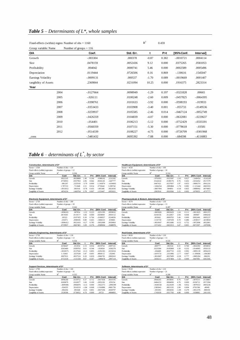
48
Whole sample, determinants of D*
Fixed-effects (within) regression Number of obs = 1160 R2
0.459
Group variable: Name Number of groups = 116
D/A Coef. Std. Err. t P>t [95% Conf. Interval]
Growth -.003304 .000378 -0.87 0.382 -.0010721 .0004114
Size .0478159 .0052436 9.12 0.000 .0375265 .0581053
Profitability .004042 .0000741 5.46 0.000 .0002589 .0005496
Depreciation .0119444 .0726506 0.16 0.869 -.130616 .1545047
Earnings Volatility -.0009131 .000537 -1.70 0.089 -.0019669 .0001407
tangibility of Assets .2369844 .0231094 10.25 0.000 .1916375 .2823314
Year
2004 -.0127664 .0098949 -1.29 0.197 -.0321828 .00665
2005 -.026111 .0100248 -2.60 0.009 -.0457825 -.0064395
2006 -.0398761 .0101633 -3.92 0.000 -.0598193 -.019933
2007 -.0353433 .0103908 -3.40 0.001 -.055733 -.0149536
2008 -.0259937 .0105585 -2.46 0.014 -.0467124 -.0052749
2009 -.0426359 .0104839 -4.07 0.000 -.0632081 -.0220637
2010 -.054401 .0106213 -5.12 0.000 -.0752429 -.0335591
2011 -.0568359 .0107151 -5.30 0.000 -.0778618 -.03581
2012 -.0514339 .0108227 -4.75 0.000 -.0726709 -.0301968
_cons -.5481432 .0695392 -7.88 0.000 -.684598 -.4116883
Table 5 – Determinants of L*, whole samples
Table 6 – determinants of L*, by sector
Construction, determinants of D* Healthcare Equipment, determinants of D*
Sector = 2350 Number of obs = 120 Sector = 4530 Number of obs = 100
Fixed-effects (within) regression Number of groups = 12 Fixed-effects (within) regression Number of groups = 10
Group variable: Name R2
0.204 Group variable: Name R2
0.324
D/A Coef. Std. Err. t P>t [95% Conf. Interval] D/A Coef. Std. Err. t P>t [95% Conf. Interval]
Growth .0922145 .0659808 1.40 0.166 -.0388102 .2232392 Growth -.0791851 .0325587 -2.43 0.017 -.1440454 -.0143249
Size .0736953 .0357953 2.06 0.042 .0026128 .1447777 Size .0142414 .0188176 0.76 0.452 -.0232452 .0517279
Profitability -.881267 .2325543 -3.79 0.000 -1.343074 -.4194603 Profitability .0467421 .0237837 1.97 0.053 -.0006374 .0941216
Depreciation 1.787153 .711848 2.51 0.014 .3735642 3.200742 Depreciation -.5266254 .2985884 -1.76 0.082 -1.121444 .0681933
Earnings Volatility -.0015012 .001916 -0.78 0.435 -.005306 .0023036 Earnings Volatility -.0007494 .004091 -0.18 0.855 -.0088992 .0074003
Tangibility of Assets .4054234 .1460764 2.78 0.007 .1153447 .6955021 Tangibility of Assets .2903916 .0920566 3.15 0.002 .1070055 .4737777
Electronic Equipment, determinants of D* Pharmaceuticals & Biotech, determinants of D*
Sector = 2730 Number of obs = 180 Sector = 4570 Number of obs = 130
Fixed-effects (within) regression Number of groups = 18 Fixed-effects (within) regression Number of groups = 13
Group variable: Name R2
0.162 Group variable: Name R2
0.287
D/A Coef. Std. Err. t P>t [95% Conf. Interval] D/A Coef. Std. Err. t P>t [95% Conf. Interval]
Growth -.0096181 .007854 -1.22 0.223 -.0251395 .0059032 Growth -.0005826 .0003629 -1.61 0.111 -.0013025 .0001372
Size .0674591 .0119177 5.66 0.000 .0439069 .0910112 Size .0250556 .0122857 2.04 0.044 .000687 .0494242
Profitability .00323 .0107455 0.30 0.764 -.0180057 .0244656 Profitability .003842 .0000703 5.46 0.000 .0002446 .0005237
Depreciation .235975 .2948185 0.80 0.425 -.3466551 .818605 Depreciation .1110759 .1587639 0.70 0.486 -.2038317 .4259834
Earnings Volatility -.0006412 .0023416 -0.27 0.785 -.0052688 .0039864 Earnings Volatility -.0010047 .0031686 -0.32 0.752 -.0072896 .0052801
Tangibility of Assets .0729937 .0667401 1.09 0.276 -.0589004 .2048878 Tangibility of Assets .1571452 .0453313 3.47 0.001 .0672307 .2470596
Industry Engineering, determinants of D* Real Estate, determinants of D*
Sector = 2750 Number of obs = 130 Sector = 8630 Number of obs = 130
Fixed-effects (within) regression Number of groups = 13 Fixed-effects (within) regression Number of groups = 13
Group variable: Name R2
0.354 Group variable: Name R2
0.535
D/A Coef. Std. Err. t P>t [95% Conf. Interval] D/A Coef. Std. Err. t P>t [95% Conf. Interval]
Growth .0258447 .012034 2.15 0.034 .0019754 .0497141 Growth .000777 .002534 0.31 0.760 -.0042492 .0058032
Size .0243469 .0399703 0.61 0.544 -.054934 .1036278 Size .0223584 .0185808 1.20 0.232 -.0144965 .0592133
Profitability -.0018575 .0137943 -0.13 0.893 -.0292183 .0255034 Profitability -.004689 .0047733 -0.01 0.992 -.0095139 .0094219
Depreciation 1.15843 .3337639 3.47 0.001 .4964112 1.82045 Depreciation -.6470731 .2331906 -2.77 0.007 -1.109606 -.1845407
Earnings Volatility .0007631 .0037516 0.20 0.839 -.0066781 .0082043 Earnings Volatility -.0010687 .0037609 -0.28 0.777 -.0085284 .006391
Tangibility of Assets .0753518 .1131334 0.67 0.507 -.1490478 .2997514 Tangibility of Assets .5050213 .0707404 7.14 0.000 .3647081 .6453345
Support Services, determinants of D* Software, determinants of D*
Sector = 2790 Number of obs = 160 Sector = 9530 Number of obs = 210
Fixed-effects (within) regression Number of groups = 16 Fixed-effects (within) regression Number of groups = 21
Group variable: Name R2
0.555 Group variable: Name R2
0.200
D/A Coef. Std. Err. t P>t [95% Conf. Interval] D/A Coef. Std. Err. t P>t [95% Conf. Interval]
Growth .0096268 .0259752 0.37 0.712 -.0417658 .0610195 Growth .0044245 .0058041 0.76 0.447 -.0070311 .0158801
Size .0269679 .0162677 1.66 0.100 -.0052181 .059154 Size .0404153 .0084836 4.76 0.000 .0236712 .0571594
Profitability -.4009386 .0966876 -4.15 0.000 -.5922373 -.2096399 Profitability -.0438158 .0223639 -1.96 0.052 -.0879553 .0003236
Depreciation -.924355 .5016519 -1.84 0.068 -1.916886 .0681756 Depreciation .2383043 .0821535 2.90 0.004 .0761586 .40045
Earnings Volatility -.004204 .001668 -0.25 0.801 -.0037206 .0028797 Earnings Volatility -.003393 .0004045 -1.09 0.279 -.0012376 .000359
Tangibility of Assets .3528596 .0736052 4.79 0.000 .20723 .4984893 Tangibility of Assets .1745039 .0357783 4.88 0.000 .1038885 .2451193

49
Construction, Speed of adjustment by size Construction, Speed of adjustment by size
Sector = 2350 Sector = 2350
Number of obs = 120 Number of obs = 120
R2
= 0.073 R
2 =
0.109
D/A Coef. Std. Err. t P>t [95% Conf. Interval] D/A Coef. Std. Err. t P>t [95% Conf. Interval]
ADJ .1077986 .0738764 1.46 0.147 -.0385229 .2541201 ADJ -.0195477 .0763481 -0.26 0.798 -.1707648 .1316694
large_cap 0 (omitted) large_cap .1585989 .1029446 1.54 0.126 -.0452958 .3624936
mid_cap .0409564 .0944124 0.43 0.665 -.1460392 .227952 mid_cap .2238381 .1003364 2.23 0.028 .0251093 .4225669
small_cap -.1635309 .1139867 -1.43 0.154 -.3892959 .0622341 small_cap 0 (omitted)
_cons .0111149 .0066585 1.67 0.098 -.0020732 .024303 _cons .0061062 .0058348 1.05 0.298 -.0054505 .0176628
Electronic Equipment Electronic Equipment
Sector = 2730 Sector = 2730
Number of obs = 180 Number of obs = 180
R2 = 0.131 R
2 = 0.107
D/A Coef. Std. Err. t P>t [95% Conf. Interval] D/A Coef. Std. Err. t P>t [95% Conf. Interval]
ADJ .2687052 .0684702 3.92 0.000 .133577 .4038335 ADJ .0721879 .1338757 0.54 0.590 -.1920204 .3363963
large_cap .0342663 .2374748 0.14 0.885 -.4343983 .502931 large_cap 0 (omitted)
mid_cap 0 (omitted) mid_cap .1176922 .1540471 0.76 0.446 -.1863251 .4217096
small_cap -.1210686 .0773008 -1.57 0.119 -.2736244 .0314873 small_cap .0903209 .1407114 0.64 0.522 -.187378 .3680197
_cons .0169005 .0073546 2.30 0.023 .002386 .031415 _cons -.0017209 .0065195 -0.26 0.792 -.0145874 .0111455
Healthcare Healthcare
Sector = 4530 Sector = 4530
Number of obs = 100 Number of obs = 100
R2 = 0.207 R
2 = 0.124
D/A Coef. Std. Err. t P>t [95% Conf. Interval] D/A Coef. Std. Err. t P>t [95% Conf. Interval]
ADJ .5611374 .1302803 4.31 0.000 .302533 .8197417 ADJ .0302408 .112506 0.27 0.789 -.1930819 .2535635
large_cap -.1871578 .2225648 -0.84 0.402 -.6289455 .2546299 large_cap 0 (omitted)
mid_cap 0 (omitted) mid_cap .3629366 .1681496 2.16 0.033 .0291622 .6967109
small_cap -.4387417 .1421366 -3.09 0.003 -.7208805 -.1566028 small_cap .0694177 .1314728 0.53 0.599 -.1915538 .3303892
_cons .015083 .0080976 1.86 0.066 -.0009906 .0311566 _cons -.003245 .0078366 -0.41 0.680 -.0188007 .0123106
Ind. Engineering Ind. Engineering
Sector = 2750 Sector = 2750
Number of obs = 130 Number of obs = 130
R2 = 0.167 R
2 = 0.085
D/A Coef. Std. Err. t P>t [95% Conf. Interval] D/A Coef. Std. Err. t P>t [95% Conf. Interval]
ADJ .086277 .0807534 1.07 0.287 -.0735317 .2460857 ADJ .1980113 .0874694 2.26 0.025 .024912 .3711106
large_cap .1575722 .1136711 1.39 0.168 -.0673796 .3825241 large_cap -.0449099 .1095711 -0.41 0.683 -.2617479 .1719282
mid_cap .204682 .1062272 1.93 0.056 -.0055384 .4149025 mid_cap 0 (omitted)
small_cap 0 (omitted) small_cap -.1280462 .1170733 -1.09 0.276 -.3597308 .1036384
_cons .0047325 .0065494 0.72 0.471 -.0082286 .0176937 _cons -.0024814 .0062514 -0.40 0.692 -.0148528 .00989
Pharma Pharma
Sector = 4570 Sector = 4570
Number of obs = 130 Number of obs = 130
R2
= 0.023 R
2 =
0.032
D/A Coef. Std. Err. t P>t [95% Conf. Interval] D/A Coef. Std. Err. t P>t [95% Conf. Interval]
ADJ .0004346 .0017963 0.24 0.809 -.0031202 .0039894 ADJ .0837978 .1188258 0.71 0.482 -.1513549 .3189506
large_cap .1366907 .1036988 1.32 0.190 -.0685261 .3419075 large_cap -.0186123 .1479719 -0.13 0.900 -.3114444 .2742197
mid_cap 0 (omitted) mid_cap .00697 .1321358 0.05 0.958 -.2545229 .2684628
small_cap -.0032865 .0032255 -1.02 0.310 -.0096697 .0030967 small_cap 0 (omitted)
_cons .0070268 .0064742 1.09 0.280 -.0057856 .0198391 _cons .0068563 .0074344 0.92 0.358 -.0078561 .0215688
Real Estate Real Estate
Sector = 8630 Sector = 8630
Number of obs = 130 Number of obs = 130
R2 = 0.163 R
2 = 0.163
D/A Coef. Std. Err. t P>t [95% Conf. Interval] D/A Coef. Std. Err. t P>t [95% Conf. Interval]
ADJ .2338475 .0637374 3.67 0.000 .1077228 .3599722 ADJ .0853443 .0625259 1.36 0.175 -.0383831 .2090717
large_cap 0 (omitted) large_cap 0 (omitted)
mid_cap -.0599633 .0624638 -0.96 0.339 -.1835678 .0636413 mid_cap .1405343 .0811258 1.73 0.086 -.0199989 .3010675
small_cap -.1210675 .0773008 -1.56 0.118 -.2736244 .0314873 small_cap -.002245 .0055366 -0.41 0.680 -.0188007 .0123106
_cons .0342125 .0120031 2.85 0.005 .0104605 .0579644 _cons -.0042277 .0086062 -0.49 0.624 -.0212578 .0128025
Software Software
Sector = 9530 Sector = 9530
Number of obs = 210 Number of obs = 210
R2 = 0.104 R
2 = 0.073
D/A Coef. Std. Err. t P>t [95% Conf. Interval] D/A Coef. Std. Err. t P>t [95% Conf. Interval]
ADJ .2338475 .0637374 3.67 0.000 .1077228 .3599722 ADJ .1873056 .0780309 2.40 0.017 .033464 .3411472
large_cap 0 (omitted) large_cap -.0546312 .1428032 -0.38 0.702 -.3361743 .2269119
mid_cap -.0599633 .0624638 -0.96 0.339 -.1835678 .0636413 mid_cap 0 (omitted)
small_cap -.1210675 .0773008 -1.56 0.118 -.2736244 .0314873 small_cap -.0522579 .0911003 -0.57 0.567 -.2318663 .1273505
_cons .0342125 .0120031 2.85 0.005 .0104605 .0579644 _cons .0025901 .0031191 0.83 0.407 -.0035595 .0087396
Support Services Support Services
Sector = 2790 Sector = 2790
Number of obs = 160 Number of obs = 160
R2 = 0.114 R
2 = 0.054
D/A Coef. Std. Err. t P>t [95% Conf. Interval] D/A Coef. Std. Err. t P>t [95% Conf. Interval]
ADJ .1298411 .0535759 2.42 0.017 .0240132 .2356689 ADJ .1094964 .0578368 1.89 0.060 -.004748 .2237408
large_cap .0322804 .2009713 0.16 0.873 -.3646957 .4292565 large_cap -.126948 .1245552 -1.02 0.310 -.3729803 .1190844
mid_cap 0 (omitted) mid_cap 0 (omitted)
small_cap .0875113 .0697992 1.25 0.212 -.0503623 .2253848 small_cap -.0224257 .0691899 -0.32 0.746 -.1590957 .1142443
_cons .0180699 .0061422 2.94 0.004 .0059372 .0302026 _cons .0001549 .0050775 0.03 0.976 -.0098747 .0101845
Table 7 – Speed of adjustment, size comparison (L* in left column & in right column)