the leverage dynamics of companies: comparison across firm

1

The leverage dynamics of companies: comparison across firm types ----An empirical study of US financial and nonfinancial firms

Master thesis in finance Tilburg School of Economics and Management

Tilburg University

Xiaodongzhang 461662

Supervisor: Prof. O. de Jonghe Second reader:

2

Abstract

Capital structure has always been a keen issue and earlier study mainly focus on the determinants of the leverage of firms. However, during the 2008 crisis, many economists notice the different characteristics of different type of firms and indicate that the leverage change differently to the asset price for different type of firms. In this paper, with systematical comparison between nonfinancial firms and financial firms, I conclude that the both of the two type of firms have procyclical leverage. This is different from the most popular view that financial firms have procyclical leverage while nonfinancial firms have counter-cyclical leverage. Moreover, this paper also indicates that the leverage adjustment speed towards optimal level is higher for financial firms. Analysis of balance sheet adjustment shows that the adjustment pattern is similar for both sectors, except that the changes in financial firms are more intense.

4

Contents

Abstract ............................................................................................................................................. 2

Introduction ...................................................................................................................................... 5

Literature Review .............................................................................................................................. 7

2.1 Determinants of capital structure in previous work. .......................................................... 7

2.2 Financial institutions and nonfinancial firms ...................................................................... 8

Research Method ............................................................................................................................ 11

3.1Empirical model ................................................................................................................. 11

3.1.1Objective ................................................................................................................. 11

3.1.2 The leverage measures ........................................................................................... 11

3.1.3 The asset size measurement .................................................................................. 12

3.1.4 The control variables .............................................................................................. 12

3.1.5 The Empirical model overview ............................................................................... 13

3.2 Sample selection and data ................................................................................................ 14

Results ............................................................................................................................................. 15

4.1 Main results ....................................................................................................................... 15

4.2 Robustness checks ............................................................................................................. 17

4.3 The adjustment speed ....................................................................................................... 19

4.4 Balance sheet adjustment for financial firms and nonfinancial firms ............................... 20

Conclusions ..................................................................................................................................... 23

Reference ........................................................................................................................................ 25

Appendix ......................................................................................................................................... 28

5

Introduction

The capital structure has drawn a great deal of attention during the 2008 financial crisis, since many financial firms, such as Lehman and Bear Stearns, deleveraged and that played a key role in turn the financial sector crisis into the global recession. In fact, since Modigliani and Miller (1958) pointed out that capital structure was related to the firm value, a lot of work has been done on the capital structure of firm. Economists figure out many determinants of the firms’ leverage ratio, including size, profitability, MTB ratio, and the firm’s fixed effect. But we should notice that, when conducting the leverage analysis, economists just pool all type of firms together, which can deviate a lot from each other in leverage management and other aspects.

Lacking proper classification of different firm type could lead us to suspect the accuracy of earlier research. As we have seen, different types of firms, including the commercial banks and nonfinancial firms, present different characteristics on leverage ratios and balance sheet management. For instance, Merton (1974) present a model of long term debt that corporation leverage fluctuates because of the changes in asset value, while the nation holding of debt keep fixed. Adrian and Shin (2014) also present a similar leverage model. Hence, leverage increase as a result of fixed debt and decreasing asset values. However, Adrian and Shin (2010, 2014) point out that this model is not a good description for the financial intermediaries leverage varies. Instead, the financial intermediaries adjust leverage through changes in the total size of the balance sheet, with equity being the exogenous variable. Consequently, financial firms will raise leverage owing to exogenous equity and growing rather than decreasing asset positions. In a word, the changes of assets influence the leverage differently for different firm types. Hence, other than the determinants noted above, it is necessary to examine how firm type affects the leverage.

This paper aims at figuring out how different firm types adjust their leverage in reaction to asset changes. It also compares their speed of adjustment and analyzes the channel through which they manage their leverage ratio towards target level. The advantage of this paper is that, I could compare firms by cross-sectional data, and also capture the each firm’s time-serial features, including the fixed effects. Moreover, unlike the Kalemli-Ozcan et al. (2012) where the aggregated leverage ratio and aggregated asset size are analyzed, I conduct the empirical study on firm and bank level. The disadvantage is that when I select samples, the survivorship bias is involved.

This paper begins with reviewing the different ideas of how the financial institutions and nonfinancial firms move their leverage to the assets size change. Adrian and Shin (2008, 2009, and 2010) show leverage patterns are countercyclical for the US non-financial sector but procyclical for investment banks. They argue that banks actively manage their balance sheet and leverage, typically through collateralized

6

borrowing and lending. Hence by utilizing surplus debt financing capacity brought by the increasing net worth, banks are going to raise their leverage. In contrast, for passive nonfinancial firms, the increasing net worth will decrease the leverage naturally. Similarly, Kalemli-Ozcan et al. (2012) document that the leverage ratio is procyclical for investment banks and large commercial banks in the US but countercyclical for nonfinancial firms. Combining precious literature on leverage issue, such as Ang, Gorovyy&Inwegen (2011) for hedge funds leverage, the current literature arrives at the agreement that the financial institutions features on procyclical leverage and nonfinancial firms features on countercyclical leverage.

However, in the previous papers, extensive attention goes to the dynamic leverage of financial sector. They provide adequate evidence for the procyclical leverage in financial sector. In contrast, the counter-cyclical leverage characteristics of nonfinancial firms are stated simply on the counter-party to financial sector. The description of the counter-cyclical leverage is simple and ambiguous. In addition to the insufficient theory, the fact that the nonfinancial firms suffered from a widespread deleveraging along with their falling assets also motivates the suspect towards the counter-cyclical leverage for nonfinancial sector. Considering that asset position can be the proxy of firm size and that for nonfinancial firms and that the firm size is strongly believed to be positively related to leverage. Rajan and Zingales (1995), Joeveer (2006) and Lemmon, Roberts, and Zender (2008) testify the significantly positive relationship. I make the first hypothesis indicating that both financial institutions and nonfinancial firms manage their leverage positively to asset position, while the leverage of former firms tends to be more sensitive.

To identify different performance of how the leverage reacts to the asset growth, I conduct the regression analysis on the U.S. financial institutions and nonfinancial firms on firm year basis from 1990 to 2013. The conclusion I draw is that both for financial and nonfinancial institutions, leverage ratio increase along with asset increase. Namely, both types of firms have procyclical leverage, and this conclusion confirms the hypothesis above.

The outcome of above empirical analysis indicates that the leverage of financial firms is more sensitive compared to nonfinancial firms, and this leads to the second hypothesis: the leverage adjustment speed is higher for financial firms. Indeed, previous literatures also approve that (0.25 for U.S. nonfinancial firms in Lemmon, Roberts, and Zender (2008), 0.21 for corporations worldwide in Oztekin and Flannery (2012), 0.29 for worldwide banks in Jonghe and Öztekin (2013), 0.4 for U.S. banks in Berger et al. (2008)). However, previous papers on leverage adjustment speed just focus on one type of firms, and there is a lack of systematic comparison between nonfinancial and financial sector. To testify the hypothesis about adjustment speed, I use the Blundell and Bond’s (1998) system GMM estimation. This estimation is a common practice in leverage adjustment issue and is considered to provide more accurate estimates in general. The estimation of leverage adjustment speed for nonfinancial firms and financial institutions are 0.40 and 0.245 respectively, both significant at 1% level.

7

What contributes to the difference in leverage adjustment? To figure out the reason, in next part, I compare the mechanisms of the balance sheet adjustment for each type of firms. Following the common practice in pervious literatures about leverage adjustment, I carry on with the partial adjustment model. Substituting target leverage ratio as a function of a vector of factors, such as the market to book ratio, the profitability and tangibility and the firm size, I derive the estimation of the adjustment speed as well as a set of the coefficients for the factors noted above. Using the outcomes, I calculate the gap between target leverage and the current level. Within each type of firms, I classify the firms into the lower gap group, middle gap group and higher gap group, which represent overleveraged firms, firms with optimal target level, and underleveraged firms respectively. Within each group, I calculate the growth for leverage, asset, debt, equity and other components of balance sheet. Comparing the values of lower group with the middle group, I could derive how the overleveraged firms to reduce leverage to be in line with their target level. Similarly, comparison of higher leverage gap group with the middle group provides how the overcapitalized firms lever up. The conclusion is that financial firms and nonfinancial firms share the almost same channel to manage leverage ratios, except that the financial firms generally make more intense changes.

On the whole, the conclusion I derive in this paper is that both financial firms and nonfinancial firms adjust their leverage positively to the asset changes, but the leverage of financial firms are more sensitive to the asset changes. Put another way, financial firms manage their leverage levels more efficiently, and it takes less time for them to achieve their target leverage ratio. In this paper, nonfinancial firms take 2.47 years to half their leverage gaps, while financial firms only spend 1.36 years to half leverage gaps.

Literature Review

Extensive work has been done on the capital structure since Modigliani and Millers’ pioneering work on capital structure, which creatively indicates that the capital structure will influence firm value. Since then, the following researches examine the determinants of the optimal capital structure by looking at different leverage level across firms. The research later is extended to dynamic analysis, to capture the firms fixed effects. They document that capital structure is determined largely by the firms fixed effect, and the firms’ leverage is quite stable to time. Recently, after the 2008 crisis, economists focus on how the different types of firms adjust their leverage ratios and balance sheet size.

2.1 Determinants of capital structure in previous work.

Modigliani and Miller (1958) point out that, with the existence of uncertainty, the decisions of debt financing and equity financing will affect the distribution of the outcome distributions. They build a theory to analyze the how the cost of capital can influence the market value under the uncertainty, and find that more debt financing will increase the expected returns, even though it will bring more dispersion. However,

8

in their theory, the choice of optimal capital structure is under a static and partial equilibrium, which should be extended to a more realistic circumstance.

Titman and Wessels (1988) testify the existing theories at that time of through empirical analysis, and they found that the “uniqueness” of the firm, the size, and profitability are the determinants of capital structures. However, whether these determinants are limited to a certain region, or it is a universal principal remains unknown. Rajan and Zingales (1995) extend their research from US to other G7 countries, and they show that the determinants are the same as above, and that there are difference in the leverage ratio in different country, and this may be because of the regulation rules. Frank and Goyal (2004) study the leverage determinants through the analysis of the publicly traded U.S. firms from 1950 to 2000. In addition to the determinants such as collateral, log of asset, expected inflation, the market-to-book ratio, profits, and dividend payment, they indicate that the average leverage level is different across industry, and it is related to the different industry nature. So in their analysis, the median industry leverage serves as another determinants, and it is positively related to the leverage ratio. Lemmon, Roberts, and Zender (2008) conduct a dynamic analysis, concluded that more than 90% of the variation in leverage is captured by firm-fixed effects while the determinants identified by the previous cross-sectional literature only account for 10% of the variation—leverage is remarkably stable over time for listed non-financial firms.

2.2 Financial institutions and nonfinancial firms

All the work so far mainly deals with the determinants of the firm’s leverage, with no classification of the firm’s type. However, the lessons from 2008 crisis make economists begin to notice different behaviors of leveraged institutions and nonfinancial firms. Greenlaw, Hatzius, Kashyap and Shin (2008) blame on the credit losses of leveraged financial intermediaries for the 2008 crisis, which is different from the previous crisis. The advantage of this paper lies in identifying the different asset classes and their main holders, and concludes that in the early stage of the financial crisis, only the mortgage backed securities and other asset backed securities suffered from the turmoil, with some asset class keeps unaffected. The former asset classes, including MBS and other ABS, are mainly held by the leveraged institutions, while the latter asset classes, including equity securities, high-yield bond and sovereign debt are mainly invested by the households. Consequently, this paper hints that the financing sector and nonfinancial firms deserve attention respectively for their performance and behavior during the 2008 crisis period. Adrian and Shin (2008, 2009) show that leverage patterns are countercyclical for the US non-financial sector but procyclical for investment banks. Banks actively manage their balance sheet and leverage, typically through collateralized borrowing and lending. In contrast, the nonfinancial firms tend to be passive facing the asset price change. They define the leverage ratio as asset divided by equity. When the net worth price and so does the asset price increase, banks will increase their debt financial to utilize the surplus capital. The much more newly issued debt compared to net worth increase will lead to

9

higher leverage ratio, which is calculated as the asset divided by equity. However, the nonfinancial firms will not act so actively, the increasing net worth will decrease the leverage ratios. Adrian and Shin (2010) point out that, for broker and dealers, the balance sheets are marked to market and the changes in net worth will be reflected in asset price immediately. That will lead to the adjustment of repos, which makes the leverage of financial intermediary procyclical. Moreover, this paper also concludes that the procyclical leverage of financial firms will lead to an amplification effects on financial cycle. Kalemli-Ozcan et al. (2012) study the capital structure across banks, firms and countries. They review the leverage and asset changes at sector level data from the Flow of Funds accounts compiled by the US Federal. They document that the leverage ratio is procyclical for investment banks and large commercial banks in the US but countercyclical for nonfinancial firms. Adrian and Shin (2014) show that leverage procyclical for broker and dealers in US. They regress leverage ratio on the VaR (value at risk), and get a significantly negative relationship between the two items. They show that financial intermediaries actively manage the capital structure according to VaR by adjusting the repos financing, and they point out the essence of adjustment is a control for the risk the investment banks will bear.

Merton (1974) put forward a model of long term debt that corporation leverage fluctuates because of the changes in asset value, while the nation holding of debt keep fixed. In his paper, the changes in asset values are mainly undertaken by equity values, and when equity size increase, which could be caused by the rising stock price, the debt holding keeps constant despite that the firms have surplus credit capacity because of the rising net worth. In this model, firms will not actively increase debt holdings with the extra credit capacity, the increasing asset tend to drag down their leverage ratio.

According to previous literature, it seems logical to conclude that financial firms seem to have procyclical leverage, while nonfinancial firms have countercyclical leverage. Alternatively, in booming economy, financial firms will add to leverage ratios through holding more debt by utilizing the surplus debt capacity, while nonfinancial firms will reduce their leverage ratio because of the rising equity and fixed debt.

Combing the firm performance during the 2008 crisis, it is not surprising to find out that most broker and dealers reduce their asset and leverage. The procyclical leverage confirms conclusion above. However, for nonfinancial firms, according to Adrian and Shin (2014) and Oztekin and Flannery (2012), the decrease asset during the recession will bring the rising leverage ratios. But the fact is that, nonfinancial firms also suffered from widespread deleveraging during the contraction. So it is reasonable to suspect the countercyclical leverage characteristics of nonfinancial firms. Considering that asset position can be the proxy of firm size and that for nonfinancial firms, and that size is testified to be positively related to leverage by Rajan and Zingales (1995), Joeveer (2006) and Lemmon, Roberts, and Zender (2008), I create my first hypothesis that both types of firms manage their leverage positively to asset changes.

10

Hypothesis 1: Financial institutions manage leverage actively, and keep a procyclical leverage ratio. Moreover, nonfinancial firms also have procyclical leverage, rather than countercyclical.

From the empirical study in this paper, an interesting discovery is that leverage of financial firms is more sensitive to the asset growth compared to nonfinancial firms. The same amount of asset growth will have greater impact on leverage of financial firms than nonfinancial ones. Indeed, the outcomes of previous literature also hints that characteristic. Lemmon, Roberts, and Zender (2008) stats that leverage is quite stable over time, and it is managed to approach their long trend target ratio. They obtain the adjustment speed of 0.25 for U.S. nonfinancial firms through the system GMM estimation. Oztekin and Flannery (2012) estimate the adjustment speed at 0.21 for corporations worldwide. For financial firms, the speed of adjustment is calculated at 0.4 for U.S. banks in Berger et al. (2008) and 0.29 for worldwide banks in Jonghe and Öztekin (2013). Apart from these empirical outcomes, Oztekin and Flannery (2012) also conclude that legal and financial traditions significantly correlate with firm adjustment speeds. The institutions with lower transaction cost have a 11% -12% faster adjustment speed than firms with higher adjustment costs. Jonghe and Öztekin (2013) obtain the consistent result that banks have heterogeneous capital structure adjustment speed, good supervisory and stringent capital requirements and better capital market could lead to a faster capital adjustment. As is known, banks are generally with less information asymmetries and high ratings, and that banks have more flexible financing source (think about the liquidity injection to commercial banks by the U.S. government during the 2008 financial crisis). All these features of financial institutions bring benefits to their adjustment cost . With this in mind, I assume that financial firms have higher adjustment speed.

Hypothesis 2: Compared that of nonfinancial firms, the leverage adjustment speed towards target level for financial institutions is higher. The time they spend to eliminate the half of leverage gap is less for financial institutions.

Through what channels do they implement leverage adjustment? Do the nonfinancial sector and financial sector shares the same pattern in adjust their balance sheet? What contributes to the difference in leverage adjustment speed? Recent literature provides various views on that issue. Adrian and Shin (2010, 2014) state that financial institutions rely on repos financing to a large extent, especially the hedge fund sector and broker and dealers, and the discount of collateral values owing to deteriorating economy may results more reduction in repos for financial firms. That to say, the reduction of repos is the main channel by which financial intermediaries achieve deleveraging. Jonghe and Öztekin (2013) analyze the balance sheet adjustment of worldwide banks, and they conclude that banks achieve deleveraging through equity growth and they lever up by the asset expansion and reduced earning rentation. To sum up their views, they both think that banks reduce leverage through active management. However, Adrian and Shin think the reduction of repos is the main source of deleveraging while Jonghe and Öztekin (2013) think the equity growth as the main reason for deleveraging. Facing the conflicting views, on one hand, it is

11

important to notice that Adrian and Shin (2010, 2014) concentrate on the five major U.S. investment banks to derive their conclusion and that the investment banks rely more on repos financing compared to commercial banks and saving unions. So it is not convincing that the the leverage management through repos adjustment of investment banks could represent the whole financial sector. On the other hand, despite Jonghe and Öztekin (2013) offer an excellent perspective of banks leverage adjustment, it is not enough to compare between financial firms and nonfinancial firms. To solve these problems, I decide to analyze how the asset, equity and debt changes of both financial institutions and nonfinancail firms.

Research Method

3.1Empirical model

3.1.1Objective

The objective of this regression analysis is to check the different influence of asset changes to leverage ratio for financial institutions and nonfinancial firms.

Instead of using the leverage ratios as dependent variable and the asset size as the independent variable, we use the logarithm of leverage ratio and logarithm of asset size. Indeed, log preferences are widely used for their tractability in models of financial intermediaries and in applications in macroeconomics. Oztekin and Flannery (2012) define the leverage as logarithm of total assets over equity and regress it on the various regulation frameworks.

But we should notice that, in the earlier analysis, the leverage ratio directly serves as the dependent variables, rather than in log format, such as Rajan and Zingales (1995), Frank and Goyal (2004) and Lemmon, Roberts, and Zender (2008). However, in these early studies, the issue of topics is the determinants of leverage like firm size, the mtb ratio, and profitability etc. These analysis does not involve the firm type into their consideration. The recent leverage study for special sector, especially for the financial sector, adopt log format to deal with their unstable basic values to promote accuracy. Considering the large amount of financial institutions in this analysis, I decide to choose the log leverage as the dependent variable. To deal with the serially correlated error items, I use the cluster analysis, which is also used in the Lemmon, Roberts, and Zender (2008). Fixed effect is also used to capture the constant heterogeneity.

3.1.2 The leverage measures

In this paper, both book leverage and market leverage are used. Adrian and Shin (2008, 2014) and Oztekin and Flannery (2012) focus on book leverage, arguing that book leverage is related to lending behavior of banks whereas the market leverage reflect how much the bank is worth to its claim holders. Gorovyy (2012) use market

12

leverage because the market equity value is closest to the NAV of a hedge fund. However, both leverage measurements are used in Lemmon, Roberts, and Zender (2008). Indeed, the two leverage measurements do not exclude, but enriches the other. The preference for different leverage measures is to perform robustness checks to see whether the leverage measures show similar results, and are therefore more reliable.

In this paper, book leverage equals total debt over book asset, while the market leverage equals the total debt over market asset, in which the market asset is the sum of total liability and market equity.

3.1.3 The asset size measurement

To match the format of leverage ratio, the independent variable is determined as the logarithm of asset. This format of asset size as an independent variable also helps to better capture the fluctuating asset of financial sectors. As is noted above, the aim of this paper is to check the relationship between the asset size and leverage ratios for different firm types, so the coefficient of asset size and its related variables are what we are most interested in. To reflect the different characteristics of financial firms and nonfinancial firms, we generate a dummy variable which equals 1 for financial firms and 0 otherwise. The interaction of the dummy variable and log asset size will present the difference between the two types of firms.

3.1.4 The control variables

In addition to log asset variable and its interaction terms with the firm type, it is necessary to include other determinants of the leverage ratios in order to improve the accuracy of the regress estimation. According to the extensive paper of optimal capital structure,the leverage level in the last period, mtb ratio, profitability, tangibility, cash flow volatility and dividends payment are the most significant ones among the leverage factors.

Lagged leverage level

The lagged leverage level is expected to be positively related with the leverage ratio. As noted in Lemmon, Roberts, and Zender (2008), the leverage for firms will keep quite stable across time, so the leverage should be mean-reverting. That means a firms with high initial leverage ratio will most likely keep a high leverage level in the following periods. Ang, Gorovyy& Inwegen (2011) also include the lagged leverage as an independent variable and obtain a significantly positive relationship. Both the initial leverage and the lagged leverage ratio emphasize the stable leverage characteristics.

Market to book ratio

Lower market to book ratio measures the fewer growth opportunities. The value firms are typically accompanied by low market to book ratio. Firms with high growth potential will utilize more equity financing and relatively less debt financing. Hence, the firms with more growth opportunities tend to be less leveraged. Market to book

13

ratio is expected to be negatively related to the leverage ratio.

Rajan and Zingales (1995), Joeveer (2006) and Lemmon, Roberts, and Zender (2008) show the significantly negative relationship. Market to book ratio is calculated as the market asset over the book asset.

Profitability

Three aspects can explain the positive relationship between profitability and leverage. First, debt provides the tax shields, so more debt goes along with higher profitability. Second, according to Jensen (1986), debt helps to supervise the mangers and hence reduce the agency cost of the company. Moreover, the firms with high profitability levels tend to borrow at lower cost, and that will lead to more debt financing.

Extensive studies (Rajan and Zingales (1995), Joeveer (2006), Haas and Peeters (2006), Lemmon, Roberts, and Zender (2008)) have indicated that the profitability is negatively related to the leverage ratio. Profitability is defined as the EBITDA over total assets.

Tangibility

Generally speaking, the more tangible assets a firm owns, the less credit risk the firm features, because the tangible assets can serve as the collateral for debt. In addition to the capacity of more debt, the tangible assets will also provide a lower debt cost, because it reduces the default risk. However, according to Shamshur (2009), the tangibility will reduce the liquidity of firms, and this will force the firm to turn to the internal financing, especially in transition economies.

Rajan and Zingales (1995), and Delcoure (2007) report that the relationship between leverage and tangibility is positive, Joeveer (2006) indicate a negative relationship. Considering the negative influence is obvious only in transition economies, its coefficient in this paper is expected to be positive. Tangibility is proxied by the PPE (Property, Plant and Equipment) over total assets

Cash flow volatility

Cash flow volatility could indicate the stability of a firm’s operating income. Generally, stable operating income could serve as a guaranty for outstanding debt and it will bring managers more risky attitude towards debt. Consequently, cash flow volatility are expected to be negatively related to leverage ratio.

Graham, Lemmon, and Schallheim (1998), Frank and Goyal (2004), Lemmon, Roberts, and Zender (2008) has testified that negative relationship.

3.1.5 The Empirical model overview

To deal with the serially correlated error items, I use the cluster analysis, which is also used in the Lemmon, Roberts, and Zender (2008). Fixed effect is also used to capture the constant heterogeneity.

We estimate the relation

14

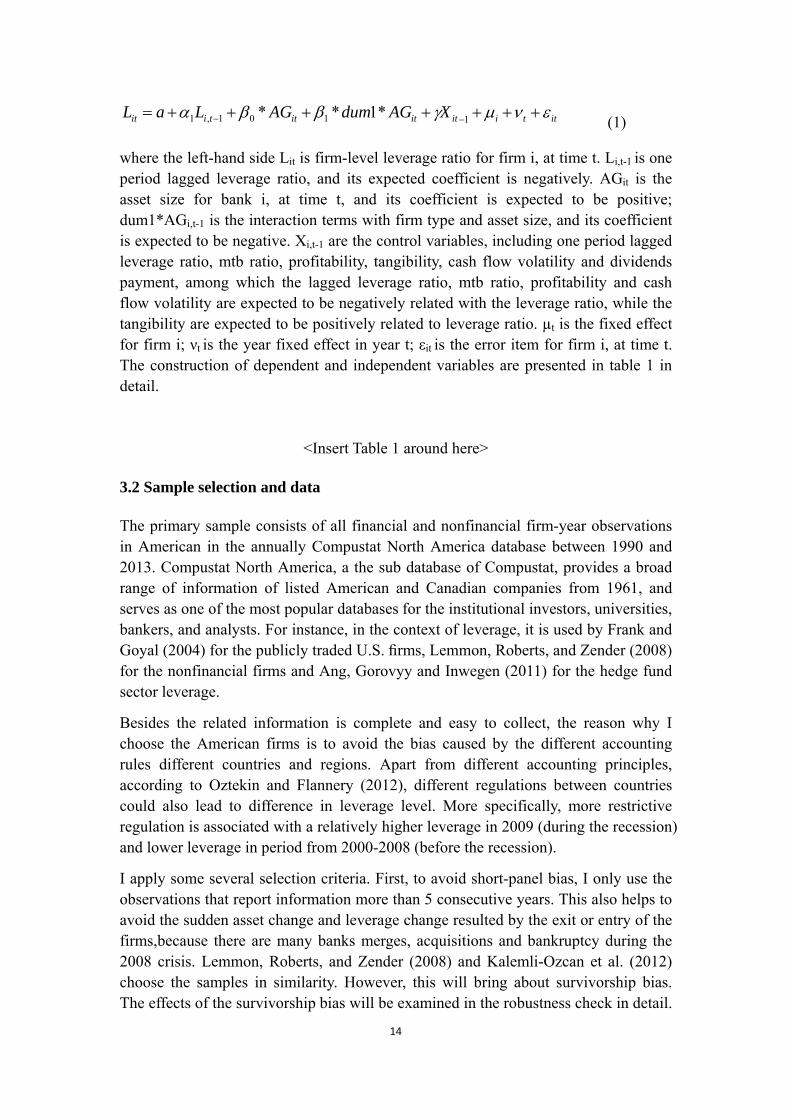
ittiititittiit XAGdumAGLaL 1101,1 *1** (1)

where the left-hand side Lit is firm-level leverage ratio for firm i, at time t. Li,t-1 is one period lagged leverage ratio, and its expected coefficient is negatively. AGit is the asset size for bank i, at time t, and its coefficient is expected to be positive; dum1*AGi,t-1 is the interaction terms with firm type and asset size, and its coefficient is expected to be negative. Xi,t-1 are the control variables, including one period lagged leverage ratio, mtb ratio, profitability, tangibility, cash flow volatility and dividends payment, among which the lagged leverage ratio, mtb ratio, profitability and cash flow volatility are expected to be negatively related with the leverage ratio, while the tangibility are expected to be positively related to leverage ratio. µt is the fixed effect for firm i; νt is the year fixed effect in year t; εit is the error item for firm i, at time t. The construction of dependent and independent variables are presented in table 1 in detail.

<Insert Table 1 around here>

3.2 Sample selection and data

The primary sample consists of all financial and nonfinancial firm-year observations in American in the annually Compustat North America database between 1990 and 2013. Compustat North America, a the sub database of Compustat, provides a broad range of information of listed American and Canadian companies from 1961, and serves as one of the most popular databases for the institutional investors, universities, bankers, and analysts. For instance, in the context of leverage, it is used by Frank and Goyal (2004) for the publicly traded U.S. firms, Lemmon, Roberts, and Zender (2008) for the nonfinancial firms and Ang, Gorovyy and Inwegen (2011) for the hedge fund sector leverage.

Besides the related information is complete and easy to collect, the reason why I choose the American firms is to avoid the bias caused by the different accounting rules different countries and regions. Apart from different accounting principles, according to Oztekin and Flannery (2012), different regulations between countries could also lead to difference in leverage level. More specifically, more restrictive regulation is associated with a relatively higher leverage in 2009 (during the recession) and lower leverage in period from 2000-2008 (before the recession).

I apply some several selection criteria. First, to avoid short-panel bias, I only use the observations that report information more than 5 consecutive years. This also helps to avoid the sudden asset change and leverage change resulted by the exit or entry of the firms,because there are many banks merges, acquisitions and bankruptcy during the 2008 crisis. Lemmon, Roberts, and Zender (2008) and Kalemli-Ozcan et al. (2012) choose the samples in similarity. However, this will bring about survivorship bias. The effects of the survivorship bias will be examined in the robustness check in detail.

15

Second, I drop the observations because of the missing data on book and marker leverage variables as well as other relevant variables (total assets, long-term debt, total liabilities, and fiscal year closing share price, fiscal year end shares outstanding, EBITDA, property, plant and equipment).Third, I drop the firm-year observations if one of the basic variables(including the book leverage, market leverage asset size and other control variables) beyond the 1% and 99% tails. Fourth, the negative leverage is not allowed here, so we drop the firms that have negative asset or negative equity during this period.

The next step is to classify the firms to two types according the NAICS (North American Industry Classification System). I define the nonfinancial sector firms as all U.S.-based companies with NAICS codes lower than 520000 or higher than 530000. Otherwise, if the NAICS fall between 520000 and 530000, it belongs to financial firms. Accordingly, I generate a dummy variable, firmtype. If a firm belongs to financial sector, the dummy variable is set at 1. Otherwise, the firms belong to the nonfinancial firms and this dummy variable are defined as 0.

The final sample has 273 financial firms with 2493 observations for the period 1990 to 2013, and 3656 nonfinancial firms with 54,830 observations.

Results

4.1 Main results

Summary Statistics

Because of firm selection criteria, it is necessary to summarize the variables for both survivors (firms report information for at least 5 consecutive years) and all firms in that period. The Summary Statistics is listed in Table 2


The quick comparison between the entire sample and survivors reveals several unsurprising differences. The average book leverage for survivors is 0.32, which is higher than that of all the firms at 0.28. The market leverage for survivors is 0.24, which is also slightly higher than that of all the firms at 0.22. In addition to the higher leverages, survivors also tend to have higher profitability level, and tangibility, but lower MTB ratios. The firms with bigger scale, higher profitability, and higher leverage are more likely to survive, which is consistent with the former study (Titman and Wessels (1988)). That will inevitably bring about survivorship bias. To eliminate this influence, I analyze the whole sample at the same time and compare its results to the survivors as robustness check. We should also notice that market leverage is more stable than book leverage (the standard deviation of book leverage is 0.39 and that of

16

market leverage is 0.19). In this case, to promote the accuracy of regression, I prefer the market leverage when calculating and comparing the leverage adjustment speed.

Correlation Matrix

To test whether this term suppressed other terms by collinearity, a correlation matrix between the variables is documented in Table 3.


The correlation matrix presents values almost all below the absolute 0.25 level. Only the interaction term Asset*firm type appear to have a high correlation with asset item. This is not strange because interaction term is constructed by the asset term. The low level correlated variables make sure the results are not affected by multi-collinearity problems.

As is noted above, the market leverage are more stable than book leverage, so the regression is mainly about the market leverage. To check the robustness, I also use the book leverage and yield a consistent result. However, owing to the limited space, the correlation matrix for book leverage is omitted.

Multivariate analyses

The regression results are presented in Table 4.


Model (1) and model (3) are the OLS regressions with year effects, and the independent variables consist of the asset size, its interaction items with the firm type, leverage ratios in last period, and the lagged control variables, including the MTB ratios, profitability, tangibility, cash flow volatility and dividends payment.

As we can see, the R-square is less than in OLS regression compared to fixed effects regression, which means OLS regression is not a proper method. In model (2) and model (4), we include the fixed effects. There is obvious improvement, especially for the market leverage model in which case the R-square increase to 0.471. The model with year effects and fixed effects captures this relationship better. This confirms Lemmon, Roberts, and Zender (2008), which concludes that, the fixed effects of firms can explain 60 percent of leverage levels, with other variables only at 10 percent.

R-square of market leverage measurement is much higher than the book leverage measurement ( 0.471 compared to 0.059). That is consistent with the high volatility of book leverage which is presented in the summary statistics.

17

The coefficient of asset size to leverage ratio for nonfinancial sectors is 0.029 measured by the book leverage, and 0.127 at market leverage, with the latter one significant at 1 % level. That for the financial firms is 0.046 (0.029+0.017) and 0.189 (0.127+0.062) respectively.

Hence, considering the higher R-square and lower standard deviation of market leverage measurement, we can conclude that, one unit asset growth will increase the leverage ratio at 0.189 units for financial firms and 0.127 for nonfinancial firms. Both the financial firms and nonfinancial firms manage their leverage ratios positively to the asset position, and the financial sector relatively adjusts their leverage levels more sensitively to the asset changes.

Another thing to notice here is the control variables, the MTB, profitability, tangibility, and the leverage level in last period. Expect for the tangibility, the leverage ratios move negatively to them. This result confirms the previous study.

4.2 Robustness checks

The robustness checks are basically OLS models and fixed effects models of all the leverage variables regressed on all the US firms selected from Compustat from 1990 to 2013. correlation matrix for all firms are presented in Table 5 and the regression results are discussed below in Table 6.


The result is similar with that of survivors. The correlation values are mainly below the absolute 0.25 level which suggest that regression outcomes will not be effected by multi-collinearity problems because of the loosely correlated variables.


Model (5) and model (6) list the leverage results measured by the book values, and model (7) and model (8) by the market values. Model (6) and model (8) include the year effects and fixed effects.

Remarkably, the results are similar with the regression on the survivors. The fixed effects model estimate the relationship between the leverage ratios and asset size better than the OLS models, and the market leverage method beats the book leverage method with higher R-square at 0.474.

The coefficient for the financial firms is 0.188, and that for the nonfinancial firms is 0.122. Compared to the results of the survivors, the effects of asset growth to leverage growth for financial firms is almost the same. However, the coefficients of control

18

variables are affected by the loose firm selection. While the signs of the variables keep consistent, they become insignificant. That indicates the exit or the new entry of some firms do reduce the accuracy of the leverage measurement.

19

4.3 The adjustment speed

Following several studies in the leverage adjustment literature, such as Flannery and Rangan (2006), Lemmon, Roberts, and Zender (2008), Faulkender, Flannery, Hankins, and Smith (2010), Jonghe and Öztekin (2013), I start with the partial-adjustment model of firm capital structure, in which the firms current leverage ratio level is weighted average of its target ratio and the last period leverage ratio.

The estimation formula:

ittiitit levlevlev 1,* )1( (2)

in which itlev is the current leverage ratio, *itlev is the target level, while the

itlev indicates the previous period leverage ratio. , the coefficient of target leverage

ratio, is the adjustment speed, and represent how fast the firm adjust their current leverage towards target level.

The target leverage is not constant over time, according to Gropp and Heider (2010), I estimate the dynamic target leverage:

1,*

tiit Xlev (3)

In which 1, tiX is a factor vector, and it includes the size, profitability, mtb ratio,

tangibility, the cash flow volatility, and the dividends payment.

Substitute the target leverage ratio into the current ratio estimation formula, we could derive:

ittitiit levXlev 1,1, )1( (4)

I regress the estimation equation above in three methods, the OLS regression with and without fixed effects, and the Blundell and Bond’s (1998) system GMM estimation. Lemmon, Roberts, and Zender (2008), Jonghe and Öztekin (2013) also use the GMM method to measure the leverage adjustment speed. The advantage of GMM methods is that it helps to cope with endogenous problem and the short time period with large cross-section firms. The OLS regression estimate a coefficient of the lagged dependent variable ( 1 in this formula) with upwards bias and the OLS regression with fixed effects will bring downward bias. The GMM estimation of 1 should be within the ranges. The results is presented in Table 7.

20


According to the estimation of 1 , the adjustment speeds for nonfinancial firms

and financial firms are 0.245 and 0.400 respectively, both significant at 1% level.

The outcome is consistent previous literature. Lemmon, Roberts, and Zender (2008) obtain the estimation at 0.25 for U.S. nonfinancial firms, and Oztekin and Flannery (2012) estimate the speed of adjustment at 0.21 for corporations worldwide. For financial firms, Berger et al. (2008) estimate it at 0.4 for U.S. banks while Jonghe and Öztekin (2013) estimate at 0.29 for worldwide banks.

Through the formula log (0.5)/log (1-adjustment speed), I derive that the nonfinancial firms need 2.47 years to half the gap between target and current leverage level, while it only takes 1.36 year for financial firms to half the gap.

Trough the partial adjustment model, I find that leverage adjustment speeds vary across different firms types. Compared to nonfinancial firms, financial institutions regulate their leverage ratio more efficiently towards their target level. This is consistent with Oztekin and Flannery (2012) and Jonghe and Öztekin (2013). They indicates that the low transaction cost associated with leverage adjustment contributes to high capital structure adjustment speed. As is known, compared to nonfinancial firms, financial firms are better informed, have more flexible funding resource, and are generally higher rated. This will definitely reduce the transaction cost to adjust their leverage ratio, and accordingly, financial firms spend less time to get close to optimal leverage ratios.

4.4 Balance sheet adjustment for financial firms and nonfinancial firms

What contributes to the difference in leverage adjustment? Why financial firms could manage their leverage more efficiently than nonfinancial firms? Do they share the same adjustment channels? In this part, I analyze and compare the mechanisms of the balance sheet adjustment for each type of firms.

To analyze firms how to increase or decrease their leverage to approach their target level, the first thing to do is to classify firms into the low leverage gap group and high leverage group. Indeed, as is described above, when I regress the equation 4 with system GMM method to get the adjustment speed, I could also calculate the optimal leverage ratio for each observation using the GMM estimators. The leverage gap is defined as the optimal value minus the current leverage,

ititit levlevgap * (5)

21

In which gap is the leverage gap, the lev* is the optimal leverage and lev is the current leverage ratio. The observations are classified into lower gap group, middle leverage group and higher gap group according to their gap values. Lower leverage gap means firms fall into that group are overleveraged, and they need to decrease their leverage level to arrive at the target level. On the contrary, the higher leverage gap means the under-leveraged firms which need to increase their leverage.

Within each group, I calculate the growth for leverage, asset, debt, equity and other components of balance sheet. Comparing the values of lower group with the middle group, I could derive how the overleveraged firms to reduce leverage to be in line with their target level. Similarly, comparison of higher leverage gap group with the middle group provides how the overcapitalized firms lever up. The conclusion is that financial firms and nonfinancial firms share the almost same channel to manage leverage ratios, except that the financial firms generally make more intense changes. The result is listed in Table 8.


In the lower gap group of panel A, the average gap is negative, which means the target leverage ratio is lower than its current ratio. The leverage growth rate is negative (-12%), and it confirms to the general knowledge that the highly leveraged firms aim to reduce the leverage ratio to be in line with its target. The asset increase around 5%, almost the same level with the middle gap group, but the debt declines at 9%, which is obviously higher than that in the middle group at 5%. Considering the formula in which I calculate the leverage ratio, leverage =debt/asset, given the approximate asset growth rate, the significant debt reduction contributes to the deleveraging.

What leads to a significant debt reduction?As is known, the debt reduction can be achieved by more debt buying back and less issuance. The table shows that the long-term debt redemption growth is large, but the debt issuance does not drop a lot compared to the middle group.Moreover, the short- term debt is falling substantially as well. So the mainly source of the falling debt are attributed to debt redemption and short-time debt reduction. Apart from debt, equity could also influence capital ratio.Actually, in the lower gap group, the equity issuance grows much faster (31% vs. 0%)and the equity repurchase declines much faster (-25% vs. -9%, the negative sign represents that the debt redeem is reducing). Both the increasing issuance and decreasing the redemption will increase equity. However,in the lower group, the equity grows only slightly faster (9%)than that in the middle group (7%), so the equity increase cannot explain different leverage growth between the two groups (because in the two groups, the equity growth rate is almost the same).

Hence, the overleveraged firms decrease their leverage ratios by less short-term debt and rapidly increasing debt redemption to keep in line with the target level.

In the higher gap group, the gap becomes positive. It means these firms are overcapitalized, so it is not surprising to obtain the positive leverage growth trend (14%) because the firms aim at levering up to meet target level. Similar with the

22

lower gap group, I investigate how these overcapitalized firms adjust their balance sheet to lever up.

The table shows that there is no asset shrink during the leveraging process. Indeed, the asset growth still remains the same level with that in the middle group, but debt growth is quite high compared to that in the middle group(19% vs. -5%). Hence, these overcapitalized firms lever up by holding more debt rather than reducing asset positions. The debt issuance is growing (10%), and it is quite different from the first two cases, in which the debt issuance is declining at high rate. However, the debt redemption growth also increases. Even though the increasing long-term debt issuance will be partly set off by the increasing debt redemption, the total long debt still grows rapidly (10%).

The equity does not shrink in the levering process. Indeed, the equity still remains increasing, but at a slower rate compared to the middle group (2% vs. 7%), and it is the result of the intense decline of both issuance and repurchase of equity.

Hence, the rapidly increasing long-term debt and short term debt promote the firms levering up.

Compared to the nonfinancial firms, the financial firms features the better management over leverage ratio, because the gap between target ratio and current leverage is smaller for each group (-5% vs. -13% in the lower group and 6% vs. 13% in higher gap group). Their leverage also changes at a higher rate than the nonfinancial firms, and that confirms to the above viewpoint that adjustment of leverage in financial sectors is more efficient. Moreover, the asset also expand more aggressively on the whole compared to nonfinancial firms, which can be attributed to the more dramatically changed equity and debt. That is possible because financial firms have more and advantages in raising capital and more flexibility. Some of them can be provide by the government, for example, the US government inject liquidity into commercial banks during the 2008 recession period.

Despite these different characteristics, they adjust their balance sheet in a similar pattern. Just like the nonfinancial firms, the overleveraged financial firms decrease their leverage ratio through intense debt reduction but not asset contraction, while the asset size remains increasing. The intense debt reduction also comes from rapidly decreasing short-term debt and increasing debt redemption. The overcapitalized firms tend to increase the debt dramatically. The difference with nonfinancial firms lies in that when they want to increase their leverage ratio, the equity issuance of financial firms does not drop a lot, but the equity repurchases increase substantially.

That confirms Jonghe and Öztekin (2013) in which they argue that the banks achieve leveraging through reduced earning retention and reserve but not genius capital downsize.

On the whole, in both nonfinancial firms and financial sectors, the firms with a relatively higher leverage ratio compared to their target level tend to decrease their leverage ratio through higher debt reduction rate and higher equity growth rate

23

compared to the firms with ideal leverage levels. However, the debt reduction speed is much higher than that in the middle group, while the equity growth speed is only slightly higher. For the underleveraged firms in both sectors, to lever up, they increase their leverage through higher debt growth and lower equity growth compared to the firms with ideal leverage levels. But during the levering up process, the asset positions present no contraction but they grow less aggressively. Even though the adjustment pattern is similar, financial firms make more intense changes in equity and debt when they try to achieve target leverage level. The outcome confirms Oztekin and Flannery (2012). They state that firms with higher adjustment speed tend to gain more external capital and they tend to make larger equity and debt adjustment compared with the slowly adjusted firms.

Conclusions

Is it countercyclical or procyclical for financial institutions and nonfinancial firms? The previous description of the leverage adjustment to the asset change for different firm type almost agree on that the investment banks and large commercial banks have procyclical leverage and nonfinancial firms have countercyclical leverage. It is considered reasonable for investment banks to manage their leverage procyclical, considering the phenomenon that during the 2008 crisis, most investment banks went through “delivering” process along with the falling asset positions. However, the conclusion about the nonfinancial firms contrasts with the fact that the nonfinancial firms also reduced asset holding and “deleveraged” during the recession—the nonfinancial firms’ leverage also procyclical.

The lack of empirical analysis on large number of samples makes the conclusion above weak and thin. Economists either use the flow fund data to describe the dynamic leverage or just focus on the major 5 broker and dealers to draw conclusion, which is not convincing enough.

This paper aims at comparing how financial firms and nonfinancial firms manage leverage ratio, their adjustment speed and what lead to that difference. The contributions of this paper are mainly in three aspects. First, the systematical comparison between financial firms and nonfinancial firms shows that both sectors adjust their leverage positively to the asset changes. Classifying the U.S. firms in the sample into financial firms and nonfinancial firms, I regress the leverage ratio on firms level and conclude that both sector manage leverage positively to asset size. This is a different view from Adrian and Shin (2014) that leverage is procyclical for financial intermediaries, while countercyclical for nonfinancial firms. Second, I also conclude that the leverage adjustment speed is higher for financail firms, and the average adjustment speed is 0.4 for U.S. financial sector, while that for nonfinanail firms at 0.245. These values of adjustment speed are in line with previous literature. Besides, as Oztekin and Flannery (2012), Jonghe and Öztekin (2013) indicate, better legal framework and capital market will reduce the transaction cost associated with leverage adjustment, and that lower adjustment cost contributes to higher adjustment

24

speed. The financial firms are generally better informed, relatively highly rated, and have flexible funding source, and are under more strict regulations, which will definitely benefits the adjustment cost, and bring about high adjustment speed. Third, as to the adjustment channels, after decompose the balance sheet adjustment, I conclude that financial and nonfinancial firms shares almost the same pattern when manage their leverage ratios. When firms aim at decreasing leverage, they will reduce debt holdings and increase equity substantially, and as a result of the mixed effects, their assets remain growing.

When firms are overcapitalized, they will increase debt, and at the same time, nonfinancial firms will decrease equity issuance but the financial institutions will not reduce the equity issuance intensely. That is consistent with Jonghe and Öztekin (2013) that banks manage actively during the deleveraging process but passively when they aim at increasing leverage. All this will shed more light on how corporations and banks manage their capital structure.

The disadvantage of this paper is that,

Besides, in the regression analysis, the median industry leverage should also be a control variable, which is done in Lemmon, Roberts, and Zender (2008). It is obvious that during nonfinancial firms, there are various industry types, and different industry also accounts partly for the firms leverage (Metz and Cantor 2006, Shamshur 2009). More work to be done to capture the industry’s role in leverage determinants of different firm type.

25

Reference

A.Beltratti, R.M.Stulz.(2012), ‘The credit crisis around the globe: Why did some banks perform better?’, Journal of Financial Economics, Vol.105 No.1, pp.1-17 A.Fostel, J.Geanakoplos. (2008), ‘Leverage cycles and the anxious economy’, The American Economic Review,Vol. 98 No. 4, pp. 1211-1244 A.Hovakimian, T.Opler, S.Titman. (2001), ‘The debt-equity choice’, Journal of Financial and Quantitative analysis,Vol. 36 No. 1, pp. 1-24 A.N.Berger, R.DeYoung, M.J.Flannery, et al. (2008), ‘How do large banking organizations manage their capital ratios?’, Journal of Financial Services Research,Vol. 34 No. 2, pp. 123-149 Caballero, Ricardo, Pablo Kurlat. (2009),‘The ‘Surprising’ Origin and B.Nature of Financial Crises: A Macroeconomic Policy Proposal,’ Massachusetts Institute of Technology Working Paper. D.Berkowitz, K.Pistor, J.F.Richard. (2003), ‘Richard J F. Economic development, legality, and the transplant effect’, European Economic Review,Vol. 47 No. 1, pp. 165-195 Diamond, Douglas, Philip Dybvig. (1983),‘Bank Runs, Deposit Insurance and Liquidity’, Journal of Political Economy, Vol. 99, No. 3, pp. 401–19 F.Allen, E.Carletti, R.Marquez. (2011), ‘Credit market competition and capital regulation’, Review of Financial Studies,Vol. 24 No. 4, pp. 983-1018 F.Modigliani, M.H.Miller.(1958), ‘The Cost of Capital, Corporation Finance and the Theory of Investment’, The American Economic Review, Vol. 48 No. 3, pp. 261-297 Gatev, Evan, Phillip Strahan. (2006),‘Banks’ Advantage in Supplying Liquidity: Theory and Evidence from the Commercial Paper Market’, Journal of Finance, Vol. 61, No. 2, pp. 867–92. G.Gorton, A.Metrick. (2012), ‘Securitized banking and the run on repo’, Journal of Financial Economics,Vol. 104 No. 3, pp. 425-451 Gaud, Philippe, et al.(2005), ‘The capital structure of Swiss companies: an empirical analysis using dynamic panel data.’, European Financial Management, Vol. 11 No. 1, pp.51–69 I.A.Strebulaev. (2007), ‘Do tests of capital structure theory mean what they say?’, Journal of Finance,Vol. 62 No. 4, pp. 1747-1787 J.C.Rochet. (1992) ‘Capital requirements and the behavior of commercial banks’. European Economic Review, Vol. 36, pp. 37–78 J.W.Hardin, H.Schmiediche, R.J.Carroll. (2003), ‘Instrumental variables, bootstrapping, and generalized linear models’, Journal of Financial Economics,Vol. 3 No. 4, pp. 351-360 Michael L.Lemmon, Michael R. Roberts, and Jaime F. Zender.(2008), ‘Back to the beginning: persistence and the cross‐section of corporate capital structure’, The Journal of Finance,Vol. 63 No. 4,pp. 1575-1608 M.J.Flannery, K.P.Rangan. (2006), ‘Partial adjustment toward target capital

26

structures’, Journal of Financial Economics,Vol. 79 No. 3, pp. 469-506 M.K.Brunnermeier, L.H.Pedersen L H. (2009), ‘Market liquidity and funding liquidity’, Review of Financial studies,Vol. 22 No. 6, pp. 2201-2238 M.Koehn, A.Santomero. (1980) ‘Regulation of bank capital and portfolio risk’, Journal of Finance, Vol. 35, No. 2, pp.35–44 M.T.Leary, M.R.Roberts. (2010), ‘The pecking order, debt capacity, and information asymmetry’, Journal of Financial Economics,Vol. 95 No. 3, pp. 332-355 M.Z.Frank, V.K.Goyal. (2009), ‘Capital structure decisions: which factors are reliably important?’, Financial Management,Vol. 38 No. 1, pp. 1-37 J.Geanakoplos.(2010), ‘The leverage cycle’, NBER Macroeconomics Annual 2009, Vol.24, pp.1–65 J.R.Graham, C.R.Harvey. (2001), ‘The theory and practice of corporate finance: evidence from the field’, Journal of Financial Economics,Vol. 60 No. 2, pp. 187-243 Ö.Öztekin , M.J.Flannery. (2012), ‘Institutional determinants of capital structure adjustment speeds’, Journal of Financial Economics,Vol. 103 No. 1, pp. 88-112 R.Blundell, S.Bond. (1998), ‘Initial conditions and moment restrictions in dynamic panel data models’, Journal of econometrics,Vol. 87 No. 1, pp. 115-143 R.C.Merton. (1974), ‘On the pricing of corporate debt: The risk structure of interest rates’, The Journal of Finance,Vol. 29 No. 2, pp. 449-470 R.Gropp, F.Heider. (2010), ‘The Determinants of Bank Capital Structure’, Review of Finance,Vol. 45 No. 2, pp. 175-210 R.Huang, J.R.Ritter. (2009), ‘Testing theories of capital structure and estimating the speed of adjustment’, Journal of Financial and Quantitative analysis,Vol. 44 No. 2, pp. 237-271 R.Haas, M.Peeters.(2006) ‘The dynamic adjustment towards target capital structures of firms in transition economies’, Economics of Transition,Vol.14 No.1, pp.133-169 S.C.Myers, N.S.Majluf. (1984), ‘Corporate financing and investment decisions when firms have information that investors do not have’, Journal of Financial Economics,Vol. 13 No. 2, pp. 187-221 S.C.Myers. (1984), ‘The capital structure puzzle’, Journal of Finance ,Vol. 39 No. 3, pp. 574-592 S.Kalemli-Ozcan, B.Sorensen, S.Yesiltas.(2012) ‘Leverage across firms, banks, and countries’, Journal of international Economics, Vol. 88 No. 2, pp. 284-298 T.Adrian, H.S.Shin.(2008), ‘Financial intermediary leverage and value-at-risk’, Staff Report,Federal Reserve Bank of New York, No.338 T.Adrian, H.S.Shin.(2010), ‘Liquidity and leverage’, Journal of financial intermediation,Vol. 19 No. 3,pp. 418-437 T.Adrian, H.S.Shin.(2014), ‘Procyclical leverage and value-at-risk’, Review of Financial Studies,Vol. 27 No. 2,pp. 373-403 Titman, Sheridan, R.Wessels.(1988), ‘The determinants of capital structure choice’, The Journal of financeVol. 43 No.1, pp.1-19 U.Bhattachary, H.Daouk, M.Welker. (2003), ‘The world price of earnings opacity’, The Accounting Review,Vol. 78 No. 3, pp. 641-678 W.Xiong. (2001) ‘Convergence trading with wealth effects: an amplification

27

mechanism in financial markets’,Journal of Financial Economics, Vol. 62, No. 2, pp. 47–92 V.V.Acharya, L.H.Pedersen. (2005), ‘Asset pricing with liquidity risk’, Journal of Financial Economics,Vol. 77 No. 2, pp. 375-410 Z.He, A.Krishnamurthy. (2011), ‘A model of capital and crisis, The Review of Economic Studies,Vol. 123 No. 2, pp. 15-36

28

Appendix

Table 1 the construction of dependent and independent variables Lit (log leverage ratio) Equals to log debt minus of log asset. Book leverage= log(total

debt)-log(book asset) Market leverage=log(total debt)-log(market asset) , in which the market asset= market equity+total liability

Li,t-1 (lagged leverage ratio) Obtained from lagged leverage ratio. AGit (log asset size ) Equals logarithm of asset size. AG=log(asset) dum1*AGi,t-1 (interaction terms)

The interaction terms with firm type and asset size. dum1=1 for financial firms and 0 for nonfinanical firms.

Mtbit (market to book ratio) Equals to the market asset to book asset. Mtb ratio serves as a control variable.(MTB =market asset/book asset)

Proit (profitability) defined as the ratio of earnings before interest, tax, depreciation, and appreciation to asset (profitability=EBITDA/asset)

Tanit (tangibility) Calculated as Property, Plant and Equipment divided by asset (tangibility=PPE/asset).

Cfvit(cash flow volatility) Calculated as the standard deviation of the three period operating income before depreciation divided by the average operating income level.

Dpit(dividends payment) Defined as 1 if there is dividends payment or 0 if there is no dividends payment

µt (fixed effects) The fixed effects terms, it is coded 1 for the each indiviadul ít (year effects) Year dummies, generate a year dummy for each quarter, and

coded 1 if the year match the observation, 0 otherwise. εit (error items) Error items for firms i, at time t.

29

Table 2. Summary Statistics

The sample consists of all firms in the Compustat database from 1990 to 2013. Thetable presents

variable averages, minimum values, the values at 25 percent, medians, the values at 75 percent, the

maximum valuesand standard deviations (SD) for the entiresample (All Firms) in panel A, as well as

the subsample of firms required to survive for at least 10 consecutive years(Survivors) in panel B.

Panel A:

All Firms

Variable Mean S.D. Min P25 Median P75 Max Book leverage 0.28 0.18 0 0.14 0.27 0.38 1.02

Market leverage 0.22 0.17 0 0.08 0.19 0.31 0.81

Log(asset) 6.65 1.93 0.35 5.34 6.74 8.06 10.54

Market-to-book 1.26 0.91 0.17 0.75 1.01 1.48 16.25

Profitability 0.14 0.07 0 0.09 0.13 0.18 0.49

Tangibility 0.36 0.25 0 0.15 0.3 0.56 0.9

Cash flow volatility 0.65 1.39 0.12 0.02 0.25 0.55 15.61

dividend payments 0.41 0.49 0 0 0 1 1

Obs. 99,830

Panel B

Survivors

Variable Mean S.D. Min P25 Median P75 Max Book leverage 0.32 0.39 0 0.09 0.25 0.41 5.63

Market leverage 0.24 0.19 0 0.05 0.16 0.32 0.8

Log(asset) 4.83 2.39 0.66 3.14 4.8 6.54 10.51

Market-to-book 2.16 4.37 0.17 0.77 1.14 1.99 94.65

Profitability 0.15 0.61 0 -0.01 0.09 0.15 0.44

Tangibility 0.29 0.24 0 0.09 0.21 0.43 0.92

Cash flow volatility 0.66 1.4 0.13 0.02 0.26 0.57 15.91

dividend payments 0.4 0.49 0 0 0 1 1

Obs. 57,323

30

Table 3 correlation matrix for survivors The sample consists of the survivors (report information at least 5 consecutive years) in the Compustat

database from 1990 to 2013. Here list the correlation matrix of log market leverage, log asset size, the

interaction term between the asset size and firm type, the 1-period lagged book leverage, market to

book ratio, profitability and tangibility. Legend *, **, and *** means p<0.05, p<0.01, p<0.001.

correlation matrix for survivors

Market leverage

asset asset*firm

type Lagged leverage

MTB Profitability Tangibility

Market leverage

1

Asset 0.1003* 1

Asset*firm type

-0.0260* 0.1475* 1

Lagged leverage

0.8344* 0.1081* -0.0247* 1

MTB -0.0207* -0.0439* -0.007 -0.0215* 1

Profitability 0.2614* 0.2125* -0.1820* 0.2834* -0.0094 1

Tangibility 0.0098 0.0452* 0,08 0.0118* -0.7735

* 0.01 1

31

Table 4 Multivariate analyses This table reports regressions for the determinant of leverage of the financial firms and nonfinancial

firms in America. The panel data is obtained from Compustat from 1990 to 2013 and it is regressed on

the survivors. The dependent variable is log leverage ratio. The regression is conducted by both book

leverage and market leverage. Column 1 and 2 is regressed on book leverage and Column 3 and 4 is on

market leverage. Column 1 and 3 are the OLS regression for the pooled sample. Columns 2 to 4 are

fixed effects panel regressions with year effects.All columns use clustered standard errors at the firm

level. Legend *, **, and *** means p<0.05, p<0.01, p<0.001, namely it denote significance at the 10 %,

5 %, and 1 % levels, respectively.

Survivors

Independent Variable

Book Leverage Market Leverage

1 2 3 4

Constant -2.400*** -2.317*** -3.848*** -3.806***

Asset 0.023*** 0.029 0.050*** 0.127***

Asset*firm type 0.000 0.017 0.012 0.062

lagged leverage 0.015** 0.011* 5.695*** 3.594***

MTB -0.002* 0.000 -0.001* 0.000

Profitability -0.004* -0.003* -0.003* -0.001

Tangibility 1.461*** 1.020*** 0.559*** 0.509***


0.000 0.000 0.000 0.000

Dividends payment

0.000*** 0.000* 0.000*** 0.000

Year effects Yes Yes Yes Yes

Fixed Effects Yes Yes

R-Square 0.066 0.059 0.437 0.471

32

Table 5 correlation matrix for all firms The sample consists of all U.S. firms in the Compustat database from 1990 to 2013. Here list the

correlation matrix of log market leverage, log asset size, the interaction term between the asset size and

firm type, the 1-period lagged book leverage, market to book ratio, profitability and tangibility. Legend

*, **, and *** means p<0.05, p<0.01, p<0.001. correlation matrix for all firms

Market leverage

asset asset*firm

type Lagged leverage

MTB Profitbility Tangibility

Market leverage

1

Asset 0.1444* 1

Asset*firm type

-0.0073 0.1573* 1

Lagged leverage

0.8230* 0.1409* -0.0111* 1

MTB -0.0118* -0.0253* -0.007 -0.0153* 1

Profitability 0.2653* 0.1956* -0.1807* 0.2887* -0.0089* 1

Tangibility 0.0073 0.0456* 0,08 0.0143* -0.2570* 0.02* 1

33

Table 6 Robustness checks with all firms This table reports regressions for the determinant of leverage of both financial firms and nonfinancial

firms in America. The panel data is obtained from Compustat from 1990 to 2013. It is regressed on the

entire sample. The dependent variable is log leverage ratio. The regression is conducted by both book

leverage and market leverage. Column 1 and 2 is regressed on book leverage and Column 3 and 4 is on

market leverage. Column 1 and 3 are the OLS regression for the pooled sample. Columns 2 to 4 are

fixed effects panel regressions with year effects. All columns use clustered standard errors at the firm

level. Legend *, **, and *** means p<0.05, p<0.01, p<0.001, namely it denote significance at the 10 %,

5 %, and 1 % levels, respectively.

All firms

Independent Variable

Book Leverage Market Leverage

1 2 3 4

Constant -2.362*** -2.249*** -3.843*** -3.778***

Asset 0.014* 0.017 0.049*** 0.122***

Asset*firm type 0.002 0.010 0.012 0.066

lagged leverage 0.014** 0.008 5.677*** 3.575***

MTB -0.001* 0.000 -0.000* 0.000

Profitability -0.003** -0.002** -0.002** -0.001

Tangibility 1.460*** 1.007*** 0.562*** 0.505***


0.000 0.000 0.000 0.000

Dividends payment

0.000*** 0.000*** 0.000*** 0.000*

Year effects Yes Yes Yes Yes

Fixed Effects Yes Yes

R-Square 0.064 0.065 0.436 0.474

34

Table 7 the adjustment speed for financial and nonfinancial firms This table reports regressions for the determinant of leverage of both financial firms and nonfinancial

firms in America. The annual panel data is obtained from Compustat from 1990 to 2013. It is regressed

on survivors (firms report information at least for 5 consecutive years). Considering its lower standard

deviation and higher R-square when compared to book leverage, we choose the market leverage as

dependent variable. The regression is conducted through three models: the OLS regression without

fixed effects, the OLS regression with fixed effects, and GMM regression. The first three columns are

regressed on nonfinancial firms and the latter three columns are financial firms. Column 1 and 4 are

OLS regression without fixed effects, and Column 2 and 5 are OLS regression with fixed effects,

Column 3 and 6 represent the outcomes for GMM regression. Legend *, **, and *** means p<0.05,

p<0.01, p<0.001, namely it denote significance at the 10 %, 5 %, and 1 % levels, respectively.

Nonfinancial firms finanical firms

Variable OLS fixed effects

GMM

OLS fixed effects

GMM

Asset 0.001** 0.019*** 0.007*** -0.003** 0.008* -0.002***Lagged leverage ratio 0.826*** 0.533*** 0.755*** 0.853*** 0.474*** 0.600*** MTB 0.000 0.000** 0.007*** 0.001 0.001* 0.003*** Profitability 0.000 0.000 0.024*** 0.000 -0.001 0.026*** Tangibility 0.020*** 0.016** -0.067*** 0.015 0.010 0.019*** Cash flow volatility 0.000 0.000 0.000** 0.000 0.000 -0.001***dividends payment -0.000*** 0.000 0.000 0.000 0.000 0.000*** constant 1.079*** 2.821*** 2.278*** 1.153 0.405 0.353*** Year effects yes yes yes yes yes yes fixed effects No Yes No No Yes No R-square 0.70 0.69 0.74 0.70

35

Table 8 balance sheet adjustment

This table reports balance sheet changes during the deleveraging and leveraging up process for both

financial firms and nonfinancial firms. The sample is obtained from the Compustat from 1990 to 2013

and consists of the U.S. survived firms (firms that report information for at least 5 consecutive years).

The first three columns list the mean values of basic variables in the lower leverage gap, middle

leverage gap and higher leverage gap group respectively. Basic variables in this part include the

leverage gap, the asset growth rate, equity growth rate, debt growth rate. It also include the issuance

and repurchase growth rate of equity and debt. The last two columns list the the significant level of

t-test for the lower v.s. middle gap group and higher gap group v.s. middle gap group. Panel A shows

the balance sheet adjustment of nonfinancial firms while panel B shows that of financial firms.

Panel A: nonfinancial firms

Variables

Lower

gap

Middle

gap

Higher

gap

Lower v.s.

Middle

gap

Higher v.s.

Middle

gap (mean) (mean) (mean)

Gap -0.13 -0.01 0.13 *** ***

Leverage -12.00% -9.00% 14.00% *** ***

Asset 5.00% 6.00% 5.00% *** ***

Equity 9.00% 7.00% 2.00% *** ***

Total debt -9.00% -5.00% 19.00% *** ***

Equity issuance 31.00% 0.00% -22.00% *** ***

Equity repurchase -25.00% -9.00% -18.00% *** ***

Debt issuance -48.00% -39.00% 7.00% *** ***

Debt repurchase 9.00% -11.00% 10.00% *** ***

Long-term debt -9.00% -10.00% 12.00% *** ***

Short-term debt -13.00% -2.00% 30.00% *** ***

Panel B: financial firms

Variables

Lower

gap

Middle

gap

Higher

gap

Lower v.s.

Middle

gap

Higher v.s.

Middle

gap (mean) (mean) (mean)

Gap -0.05 0.00 0.06 *** ***

Leverage -16.00% -4.00% 19.00% *** ***

Asset 10.00% 8.00% 7.00% *** ***

Equity 13.00% 10.00% 5.00% *** ***

Total debt -8.00% 2.00% 26.00% *** ***

Equity issuance 5.00% -6.00% -7.00% *** ***

Equity repurchase -19.00% -8.00% 26.00% *** ***

Debt issuance -58.00% -58.00% 8.00% *** ***

Debt repurchase 8.00% -15.00% -1.00% *** ***

Long-term debt -2.00% 17.00% 14.00% *** ***

Short-term debt -17.00% 3.00% 25.00% *** ***

the leverage dynamics of companies: comparison across firm

Documents