the role of volatility in forecasting

Review of Accounting Studies, 7, 195–215, 2002©C 2002 Kluwer Academic Publishers. Manufactured in The Netherlands.

The Role of Volatility in Forecasting

BERNADETTE A. MINTON [email protected] State University

CATHERINE M. SCHRAND∗ [email protected] of Pennsylvania

BEVERLY R. WALTHER [email protected] University

Abstract. Theories of underinvestment propose a link between cash flow volatility and investment and subsequentcash flow and earnings levels. Consistent with these theories, our results indicate that forecasting models that includevolatility as an explanatory variable have greater accuracy and lower bias than forecasting models that excludevolatility. The improvement in forecast accuracy and bias is greatest when the firm is most likely to experienceunderinvestment. The profitable implementation of a trading strategy based on these findings, however, suggeststhat equity market participants do not incorporate fully the information in historical volatility when forecastingfuture firm performance.

Keywords: cash flow, forecasting, underinvestment, volatility

JEL Classification: G31, G35, M41, G19

1. Introduction

Theories of risk management propose a relation between volatility and investment levels. Inthe presence of market imperfections, external capital is more costly than internal capital andcash flow volatility is associated with underinvestment (see Myers, 1977). Higher volatilityleads to periods in which the firm has insufficient cash flow to fund its “desired” investment.The result is a lumpy investment pattern over time and a reduction in expected futurecash flow and earnings levels (Froot, Scharfstein and Stein, 1993; Smith and Stulz, 1985).Minton and Schrand (1999) document a negative relation between cash flow volatility andinvestment, suggesting that firms with more volatile cash flows are more likely to experienceinternal cash flow shortfalls and forgo investment. Exacerbating the effect of volatility onunderinvestment is the fact that firms with more volatile cash flows or earnings are morelikely to experience a greater external cost of capital (Minton and Schrand, 1999).

Despite the hypothesized link between volatility and future cash flow and earnings, fore-casting models in prior research traditionally include only historical cash flow and earnings

∗Address correspondence to: The Wharton School, University of Pennsylvania, 2427 Steinberg Hall-Dietrich Hall,Philadelphia, PA 19104.

196 MINTON, SCHRAND AND WALTHER

levels (Bowen, Burgstahler and Daley, 1986; Dechow, 1994; Finger, 1994; Sloan, 1996;Wilson, 1987). Although some studies have considered the predictive ability of particularfundamental variables such as the components of accruals (e.g., Bernard and Stober, 1989;Barth, Cram and Nelson, 2001), none have considered the role of volatility in forecastinglevels of future cash flows or earnings.

Based on the theories of risk management, we predict that volatility contains incrementalinformation for forecasts of future firm performance beyond that in historical cash flow,earnings, or investment levels. As a result, forecasts of cash flow and earnings that explicitlyincorporate historical volatility will be more accurate and less biased than forecasts frommodels that exclude volatility as an explanatory variable. We expect greater improvementsin forecasting performance from incorporating volatility in the forecasting model when afirm is more likely to experience underinvestment. Underinvestment is most likely to occurwhen return on assets is low and when noise in cash flow is high.

Empirical analysis of non-financial firms on Compustat over the period 1983–1997 con-firms these predictions. We find a statistically negative relation between volatility and futureoperating cash flow and operating income levels, even after controlling for historical cashflow, operating income, investment, or firm characteristics. Forecasting models that incor-porate historical volatility yield significantly more accurate and less biased forecasts thanforecasting models that exclude volatility. The incremental predictive power of historicalvolatility is especially pronounced for firms with high historical volatility and low return onassets. Thus, the benefit of using a more complex model is greatest when volatility affectsthe firm’s ability to fund investment.

Despite the better predictive accuracy of forecasting models that include historical volatil-ity, the market appears to ignore information on volatility in equity valuation. We documentpositive and significant hedge returns to a trading strategy that takes a long (short) positionin firms for which the forecast of future cash flow from models that exclude volatility is less(greater) than the forecasts from models which incorporate volatility. Positive hedge returnsalso result when we base the trading strategy on forecasts of future operating income. Thesesignificant hedge returns are consistent with investors ignoring the information in historicalvolatility.

Overall, the results show that investors can improve cash flow and earnings forecasts sig-nificantly, and therefore firm valuations, if they explicitly incorporate information aboutthe effect of volatility on investment and future firm performance. In this regard, ourfindings contribute to the fundamental analysis research that identifies factors that im-prove valuations (see, e.g., Abarbanell and Bushee, 1997, 1998; Lev and Thiagarajan,1993). The implications of our research, however, are not limited to predictions forequity valuation. For example, individuals must forecast cash flow levels in a varietyof other contexts, such as option pricing, debt pricing, and capital budgeting. Possibleextensions of this research include further work on how individuals incorporate the in-formation in volatility in cash flow or earnings forecasts in contexts other than equityvaluation.

The remainder of the paper is organized as follows. Section 2 outlines the paper’s pre-dictions about the role of volatility in forecasting. Section 3 examines the predictions usingempirical data. Section 4 analyzes the valuation implications of these results. Section 5concludes.

THE ROLE OF VOLATILITY IN FORECASTING 197

2. The Role of Volatility in Forecasting

2.1. The Relation between Volatility and Underinvestment

We rely on the risk management literature, and in particular the underinvestment storyof Myers (1977), to predict a negative relation between volatility and future cash flow andearnings levels. Based on models that capture underinvestment, Froot, Scharfstein and Stein(1993) and Smith and Stulz (1985) both assert a negative relation between cash flow volatilityand future cash flow performance to explain why firms engage in costly hedging strategies. Inthe presence of market imperfections, cash flow volatility decreases the likelihood that firmswill have sufficient internal capital to fund investment. Assuming external capital is morecostly than internal capital, firms with insufficient internal capital forgo investment. Theresult is that firms with higher volatility will forgo (or reduce) investment in some periods,resulting in a “lumpy” pattern of investment over time. Because the forgone investment isnot recovered in future periods (see Minton and Schrand, 1999), higher volatility leads tolower average investment, lower future cash flows, and lower future earnings through time.

Critical to the underinvestment story is the assumption that external capital is more costlythan internal capital. Thus, firms do not borrow to fully fund investment in periods of lowinternal cash flow realizations. Existing evidence supports this assumption. Empirically,firms are more likely to forgo investment when costs of accessing external capital are high.Moreover, a firm’s cost of accessing capital is positively related to its cash flow volatility(Minton and Schrand, 1999) and its earnings volatility (see, e.g., Beaver, Kettler and Scholes,1970; Gebhardt, Lee and Swaminathan, 2001). Hence, higher volatility not only increasesthe likelihood that a firm will not have sufficient internal cash available to fund investment,1

it also increases the cost of obtaining external capital to fund cash flow shortfalls.Based on these empirical results and aforementioned theories of risk management, we

predict that volatility has a negative relation with future operating cash flows and futureoperating income. Further, we predict that incorporating volatility into the forecasting modelwill result in more accurate and less biased forecasts of future cash flows and earnings.2

We also predict that the expected improvements from including volatility in the fore-casting model will be especially pronounced when a firm’s investment pattern is mostlumpy as a result of periods of underinvestment. One factor that affects the likelihood ofunderinvestment is the firm’s cash return on assets. As return on assets increases, invest-ment expenditures from prior periods generate greater future cash flows. Consequently,for a given level of prior period investment, a firm with a greater return on assets is morelikely to have sufficient internal cash flow to fund investment. Thus, we predict that theunderinvestment problem will be more severe, and thus the improvements from includ-ing volatility in a forecasting model will be greatest, as the firm’s cash return on assetsdecreases.

The growth rate in a firm’s investment expenditures will affect the likelihood that cashflow volatility affects investment in two opposing ways. As growth increases, a firm’sdesired level of investment, and thus the probability of underinvestment, increases. How-ever, operating cash flow realizations also increase as growth increases because of higherprior-period investment, reducing the likelihood of underinvestment. Therefore, the relationbetween growth and the likelihood of underinvestment is unclear ex ante.


Finally, “random” noise in cash flow will increase the probability of underinvestment.Noisier cash flows increase the likelihood that there will be insufficient cash flow to fund thedesired investment, leading to a lumpy investment pattern. Thus, the inclusion of volatilityin the forecasting model will lead to the greatest improvements for firms with higher levelsof noise in cash flow.

2.2. Alternative Explanations for a Relation between Volatilityand Future Firm Performance

In addition to the underinvestment story, the risk management literature provides severalalternative explanations for a negative association between volatility and future cash flowand earnings levels. For example, Smith and Stulz (1985) hypothesize that in the presenceof information asymmetry and risk-averse managers, volatility can increase compensationcosts, thus reducing expected cash flow levels. Smith and Stulz also hypothesize that volatil-ity will be negatively associated with future performance when taxable income volatilityleads to higher expected future tax payments due to progressive tax schedules and net oper-ating loss carryforwards. Graham and Smith (1999) empirically document that the presentvalue of a firm’s income taxes increases in the volatility of taxable income. If cash flowvolatility is associated with taxable income volatility, then higher cash flow volatility isnegatively related to after-tax cash flows.

Another explanation for a negative relation between volatility and future performanceassumes that firms with higher volatility are perceived to have a higher probability offinancial distress or a higher cost of capital. When the probability of financial distress ishigh, suppliers and customers might be unwilling to do business with a firm (Shapiro andTitman, 1986), resulting in lower future firm performance.

Extant research also indicates higher volatility reduces the information that is availableabout a firm, which in turn increases the firm’s cost of capital. For example, Waymire(1985) documents that firms with less volatile earnings more frequently issue managementearnings forecasts than firms with more volatile earnings. Alford and Berger (1999) indicatethat analysts prefer to follow firms for which earnings are easy to forecast (see also Waltherand Willis, 1999). Less information leads to lower liquidity and a higher cost of capital(Amihud and Mendelson, 1988). Empirical evidence supports the link between earningsvolatility and a firm’s cost of capital (e.g., Beaver, Kettler and Scholes, 1970; Gebhardt,Lee and Swaminathan, 2001). The documented association between volatility and a firm’scost of capital is consistent with the underinvestment story—firms forgo investment whenvolatility is high and cash flow realizations are low because it is costly to borrow to fundinvestment.

Despite these other theories on the relation between volatility and future firm performance,we focus on the underinvestment story because empirical evidence provides the most supportfor this explanation. Minton and Schrand (1999) empirically document a negative relationbetween cash flow volatility and average discretionary investment. Further, they show that apositive relation between volatility and the cost of accessing external capital exacerbates theunderinvestment problem associated with cash flow volatility. Their analysis also providesevidence that the sensitivity of investment to cash flow volatility does not result becausevolatility is a proxy for project risk.


Indirect evidence also supports the underinvestment story. Firms that use derivatives toreduce volatility have greater investment opportunities but also face liquidity constraints(e.g., Geczy, Minton and Schrand, 1997; Guay, 1999; Mian, 1996; Nance, Smith andSmithson, 1993). These firms are most likely to incur the highest costs from volatilityin the absence of any activities to reduce it. Our analysis on whether the benefits fromincorporating volatility into the forecasting model are associated with the likelihood ofunderinvestment also provides indirect evidence on the validity of the underinvestmentstory.

3. Empirical Tests of Predictions

In this section, we test the predictions about the effects of volatility on future cash flow andearnings levels. Prior literature has assessed the relevance of particular variables for fore-casting firm performance by directly examining their relation to stock returns (e.g., Dechow,1994; Francis, Olsson and Oswald, 2000). Such tests, as acknowledged by Dechow (1994),are joint tests of the relative predictive power of the forecasting models and whether marketparticipants use the more accurate model in equity valuation. We separate the joint test intotwo parts. In this section, we address the first issue: the predictive power of the forecastingmodels. In Section 4, we investigate whether market participants use the information involatility in valuation.

3.1. Sample and Empirical Proxies

The sample contains 3,501 firm-year observations for non-financial institutions from 1983to 1997 (1,076 distinct firms) with sufficient data to calculate operating cash flow, invest-ment, and operating income levels, cash flow volatility, operating income volatility, andproxies for firm characteristics as described below. Quarterly operating cash flow (OPCF)is defined as operating income before depreciation (Compustat data item 21) adjusted forworking capital accruals (see Dechow, 1994).3 We adjust this operating cash flow numberfor “investment” expenditures that are expensed as part of operating income by addingback quarterly research and development and advertising expenses, estimated as the annualresearch and development or advertising expense from Compustat divided by four.4 Oper-ating income (OPINC) is operating income before depreciation.5 We scale both OPCF andOPINC by the firm’s average total assets for the year.

We divide the sample period into 11 overlapping five-year periods (e.g., 1983–1987, 1984–1988, . . . , 1993–1997), and calculate the firm’s historical and future levels and volatilitymeasures for each period. The future (historical) level of cash flow or accounting earningsis the annual measure for the fifth (fourth) year of each five-year period.

Historical volatility is measured as the coefficient of variation over the first four years(16 quarters) in the five-year period. The coefficient of variation for operating cash flow(operating income) is the standard deviation of operating cash flow (operating income)scaled by the absolute value of the mean of operating cash flow (operating income) over thesame period. We require that a firm have data for at least 12 of the 16 quarters to calculatehistorical volatility. The coefficient of variation is a unitless measure of volatility that has


been used in prior studies (Albrecht and Richardson, 1990; Michelson, Jordan-Wagner andWootton, 1995; and Minton and Schrand, 1999).

One potential concern with using quarterly data to calculate the coefficient of variation isthat a firm’s quarterly cash flow and operating income, and therefore investment patterns,can be seasonal. Minton and Schrand (1999) document that the negative relation betweencash flow volatility and investment is not dependent on whether cash flows are seasonally-adjusted prior to measuring the coefficient of variation. Thus, to maximize the number ofavailable observations, we use unadjusted quarterly cash flow and income levels.

Another concern with this measure is that scaling by the absolute value of the meanof either cash flow or income can lead to extreme observations when the variable is nearzero. To minimize the effect of extreme observations, the coefficient of variation measures,as well as operating cash flow and operating income, are winsorized at the 1st and 99thpercentile values.

3.2. The Association between Volatility and Future Firm Performance

Table 1 presents the mean coefficient estimates and adjusted R2s for the 11 separate annualregressions that forecast operating cash flow or operating income at t + 1.6 The modelincludes historical volatility as well as operating cash flow and operating income levels.

Table 1. Regression analysis of the relation between volatility and future operating performance.

Variable OPCF Model OPINC Model

Intercept 0.0699 0.0197(6.102) (3.877)

OPCF 0.4863 0.0736(7.649) (2.359)

OPINC 0.4049 0.8567(9.380) (11.513)

CV(OPCF) −0.0043(−5.466)

CV(OPINC) −0.0023(−2.164)

Adjusted R2 60.73% 68.64%

Summary of cross-sectional, rolling window regressions of the future level of operating cash flow or operatingincome on historical operating cash flow level, historical operating income level, and historical volatility:

OPCFt+1 = δ0 + δ1OPCFt + δ2OPINCt + δ3CV(OPCF)t + ε

OPINCt+1 = δ′0 + δ′

1OPCFt + δ′2OPINCt + δ′

3CV(OPINC)t + ε′

The future levels of operating cash flow (OPCF) and operating income (OPINC) are the annual measures for thefifth year of each five-year period between 1983 and 1997, scaled by average assets. Historical OPCF and historicalOPINC are the annual measures for the fourth year of each five-year period between 1983 and 1997, scaled byaverage assets. The historical coefficient of variation as a proxy for cash flow volatility (CV(OPCF)) or earningsvolatility (CV(OPINC)) is calculated using quarterly data in the first four years of each five-year period between1983 and 1997. The mean coefficient estimate from the overlapping regressions, the Z ′ statistic in parentheses totest the hypothesis that the mean estimated coefficient equals zero, and the mean adjusted R2 are provided.


Operating cash flow (OPCF) and operating income (OPINC) are included as controls.Previous research has documented that both cash flow levels and earnings levels are incre-mentally relevant for equity valuation (e.g., Bowen, Burgstahler and Daley, 1986; Dechow,1994; Finger, 1994; Sloan, 1996; Wilson, 1987). Earnings has predictive ability becausethe accrual component of earnings provides information about future cash collections andfuture required cash payouts.

Table 1 shows that the mean coefficient estimate on historical cash flow volatility is sta-tistically negative for the model predicting future cash flows. The negative relation betweenvolatility and future cash flow is consistent with the underinvestment story.7 The coefficienton volatility is negative in ten of the 11 rolling window regressions, and significant in nineof the 11 estimations. The negative relation exists after controlling for the previously doc-umented positive relations between future cash flow and historical levels of cash flow andearnings. Thus, there is a role for volatility in forecasting future cash flow levels.

We also estimate an alternative specification of the forecasting model that includes aninteraction term, CV(OPCF)*OPCF (results not reported). This specification allows for therelation between cash flow volatility and future cash flow performance to be non-linear inthe level of a firm’s cash flow. This specification is consistent with the underinvestmentstory in that firms that have large cash flows may be able to withstand volatility shocksbetter. In the non-linear specification, the mean coefficient estimate on CV(OPCF) is notstatistically different from zero. However, the mean coefficient estimate on the interactionterm, CV(OPCF)*OPCF, is negative and significant. This finding indicates that as historicalvolatility increases, less weight should be placed on historical operating cash flow levelsfor forecasting future cash flows.

Since earnings levels are often the performance measure predicted, Table 1 also reportsthe results of a model that forecasts future operating income, rather than operating cashflow, at time t + 1. These results show that historical volatility also has a role in forecast-ing future earnings levels. The mean coefficient estimate on historical operating incomevolatility (CV(OPINC)) is statistically negative for the model predicting future operatingincome. Similar to the results for future cash flow levels, this negative association existsafter controlling for historical levels of income and cash flow.

We also estimate a regression that uses CV(OPCF) instead of CV(OPINC) to predict futureoperating income levels. This specification increases the explanatory power of the regressionfrom 68.64% to 81.80%. Furthermore, the mean coefficient estimate on CV(OPCF) remainssignificantly negative (−0.0012, Z ′ = −2.156, results not tabulated). This specificationis most consistent with the underinvestment story in which cash flow volatility affectsinvestment, which in turn affects future performance (as measured by earnings). Theseresults confirm our conclusion that historical volatility has a negative relation with futureoperating cash flow and operating income levels, consistent with the effect of volatility onthe likelihood of underinvestment.

3.3. The Role of Volatility in Alternative Forecasting Modelsof Future Firm Performance

In Table 2, we investigate whether the incremental explanatory power of volatility for futureoperating performance documented in Table 1 holds in three alternative forecasting models.


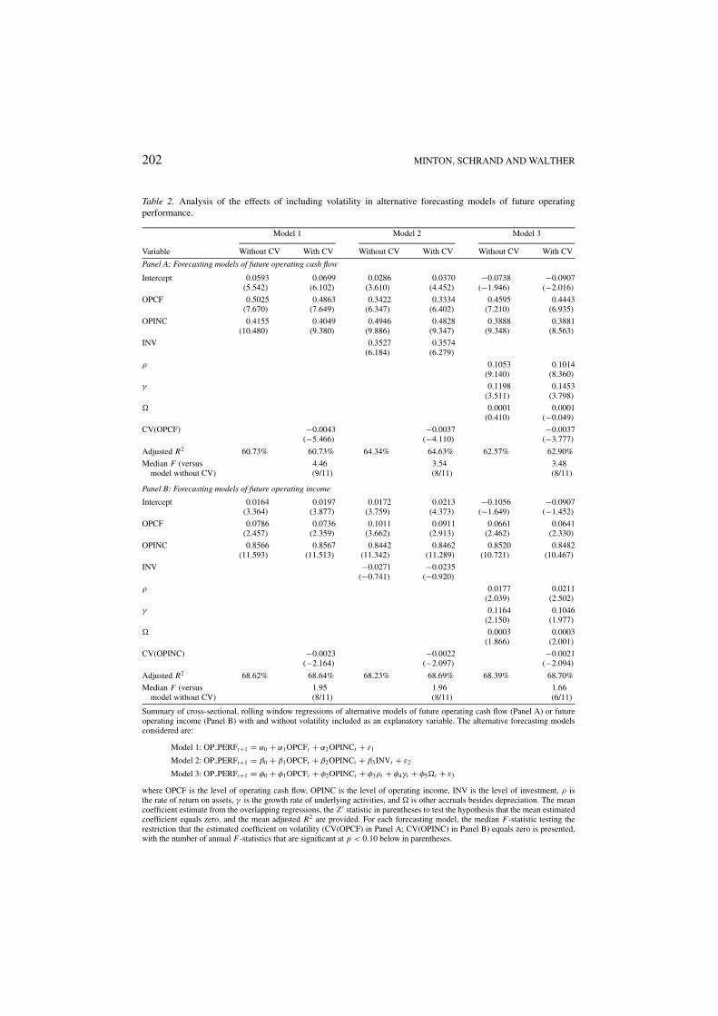
Table 2. Analysis of the effects of including volatility in alternative forecasting models of future operatingperformance.

Model 1 Model 2 Model 3

Variable Without CV With CV Without CV With CV Without CV With CV

Panel A: Forecasting models of future operating cash flow

Intercept 0.0593 0.0699 0.0286 0.0370 −0.0738 −0.0907(5.542) (6.102) (3.610) (4.452) (−1.946) (−2.016)

OPCF 0.5025 0.4863 0.3422 0.3334 0.4595 0.4443(7.670) (7.649) (6.347) (6.402) (7.210) (6.935)

OPINC 0.4155 0.4049 0.4946 0.4828 0.3888 0.3881(10.480) (9.380) (9.886) (9.347) (9.348) (8.563)

INV 0.3527 0.3574(6.184) (6.279)

ρ 0.1053 0.1014(9.140) (8.360)

γ 0.1198 0.1453(3.511) (3.798)

0.0001 0.0001(0.410) (−0.049)

CV(OPCF) −0.0043 −0.0037 −0.0037(−5.466) (−4.110) (−3.777)

Adjusted R2 60.73% 60.73% 64.34% 64.63% 62.57% 62.90%

Median F (versus 4.46 3.54 3.48model without CV) (9/11) (8/11) (8/11)

Panel B: Forecasting models of future operating income

Intercept 0.0164 0.0197 0.0172 0.0213 −0.1056 −0.0907(3.364) (3.877) (3.759) (4.373) (−1.649) (−1.452)

OPCF 0.0786 0.0736 0.1011 0.0911 0.0661 0.0641(2.457) (2.359) (3.662) (2.913) (2.462) (2.330)

OPINC 0.8566 0.8567 0.8442 0.8462 0.8520 0.8482(11.593) (11.513) (11.342) (11.289) (10.721) (10.467)

INV −0.0271 −0.0235(−0.741) (−0.920)

ρ 0.0177 0.0211(2.039) (2.502)

γ 0.1164 0.1046(2.150) (1.977)

0.0003 0.0003(1.866) (2.001)

CV(OPINC) −0.0023 −0.0022 −0.0021(−2.164) (−2.097) (−2.094)

Adjusted R2 68.62% 68.64% 68.23% 68.69% 68.39% 68.70%

Median F (versus 1.95 1.96 1.66model without CV) (8/11) (8/11) (6/11)

Summary of cross-sectional, rolling window regressions of alternative models of future operating cash flow (Panel A) or futureoperating income (Panel B) with and without volatility included as an explanatory variable. The alternative forecasting modelsconsidered are:

Model 1: OP PERFt+1 = α0 + α1OPCFt + α2OPINCt + ε1

Model 2: OP PERFt+1 = β0 + β1OPCFt + β2OPINCt + β3INVt + ε2

Model 3: OP PERFt+1 = φ0 + φ1OPCFt + φ2OPINCt + φ3ρt + φ4γt + φ5t + ε3

where OPCF is the level of operating cash flow, OPINC is the level of operating income, INV is the level of investment, ρ isthe rate of return on assets, γ is the growth rate of underlying activities, and is other accruals besides depreciation. The meancoefficient estimate from the overlapping regressions, the Z ′ statistic in parentheses to test the hypothesis that the mean estimatedcoefficient equals zero, and the mean adjusted R2 are provided. For each forecasting model, the median F-statistic testing therestriction that the estimated coefficient on volatility (CV(OPCF) in Panel A; CV(OPINC) in Panel B) equals zero is presented,with the number of annual F-statistics that are significant at p < 0.10 below in parentheses.


Model 1 is a benchmark model that includes historical operating cash flow and historicaloperating income. This forecasting model represents a specification that is traditionallyexamined in accounting research.

The second alternative model (Model 2) includes the firm’s historical investment levelin addition to the variables in the benchmark model. Historical investment may representa reasonable substitute for historical volatility with respect to its ability to forecast futureoperating performance. Investment is defined as quarterly capital expenditures plus esti-mates of quarterly research and development and advertising expenses, deflated by averageassets. Quarterly capital expenditures are estimated as the change in net property, plant, andequipment plus depreciation.8

Finally, Model 3 includes fundamental variables that drive the cash flow generation pro-cess: return on assets and growth. The cash flow return on assets variable is calculated ascash flow from operations (cash flow from operations plus cash interest paid) at year t di-vided by the value of gross PPE minus accumulated depreciation (“net PPE”) at year t − 1.The growth variable is calculated as the annual growth rate of investment opportunities,measured by net PPE at time t divided by net PPE at time t − 1.

Model 3 also includes a proxy for other accruals, . The variable is calculated asthe ratio of other accruals (defined as current assets minus current liabilities) to operatingcash flow, and captures differences between firms’ trade cycles (see Minton, Schrand andWalther, 2001). It is included in Model 3 because both operating cash flow and its derivative,operating income, are included in the model.

For each of the overlapping five-year periods, we measure return on assets, growth, andother accruals as the mean of the quarterly values for the first four years of the period. Werequire that a firm have at least 12 quarters of data to calculate each mean. Although theresults are similar if we measure these variables as the mean value over the entire five-yearperiod, measuring the characteristics over only the first four years creates a proxy that ismore consistent with the information that investors would have available for predictionpurposes. To minimize the effect of extreme observations, all of the empirical proxies arewinsorized at the 1st and 99th percentile values.

Table 2 reports the estimation results for each of the three alternative models, with andwithout cash flow volatility as an additional explanatory variable. Panel A provides theregression results for predicting future operating cash flow. Panel B provides the regressionresults for predicting future operating income.

On average, historical levels of cash flow and operating income provide reasonable esti-mates of future operating cash flow (Panel A) and operating income (Panel B)levels. The mean adjusted R2 of Model 1 for the overall sample is 60.73% for the op-erating cash flow model, and 68.62% for the operating income model. Consistent withprior research, the estimated coefficients on OPCF and OPINC are statistically positive(p < 0.02).

Historical volatility contains incremental explanatory power for future operating levelsbeyond that in historical cash flow and earnings levels, as previously documented in Table 1.Although the average overall explanatory power of Model 1 (as measured by the adjusted R2)with and without volatility is similar, the F-statistic testing the restriction that the coefficientvolatility is zero is significant in nine (eight) of the 11 annual regressions for the cash flow(income) model.


Adding historical investment to the model (Model 2) provides incremental explanatorypower for future cash flow levels relative to Model 1. The mean adjusted R2 increasesfrom 60.73% for Model 1 to 64.34% for Model 2 in Panel A. The partial F-test rejectsthe restriction that the coefficient on INV in the cash flow model equals zero at the 10%probability level in all 11 annual regressions (not reported). In Panel A, the mean estimatedcoefficient on INV is positive and statistically significant at p < 0.01, indicating that higherinvestment is associated with higher future operating cash flows. By contrast, the meanestimated coefficient on INV is insignificant in Panel B, suggesting that after controlling forhistorical cash flow and earnings levels, investment does not contain incremental explanatorypower for future operating income.

When volatility is added to Model 2, the coefficient is statistically negative and significantin both the operating cash flow and operating income models. In both panels, the partialF-test rejects the restriction that the coefficient on volatility equals zero at the 10% prob-ability level in eight of the 11 annual regressions. Therefore, historical volatility containsinformation incremental to that in historical investment for future operating performance.

Incorporating firm characteristics (Model 3) improves the predictability of future operat-ing performance, and especially operating cash flow, over Model 1. For the operating cashflow (operating income) model, the partial F-statistic rejects the restriction that the coeffi-cients on ρ, γ , and ω equal zero in ten (seven) of the 11 annual regressions (not tabulated).In both panels, the mean annual estimated coefficients on ρ and γ are positive and signifi-cant, indicating that increases in the rate of return or growth are associated with increasesin future operating cash flow and operating income levels. The mean estimated coefficienton other accruals is insignificant in Panel A, but is significantly positive in Panel B. Thepositive coefficient indicates that higher levels of other accruals are associated with higherlevels of future operating income.

In both panels, the mean coefficient on volatility is significant and negative when it isadded to Model 3. Thus, the variables that characterize the cash flow generation process donot fully capture the information about future operating performance in historical volatility.

Table 3 provides the forecast accuracy and bias statistics for the models with and with-out volatility included as an explanatory variable. This comparison allows us to assesswhether adding volatility to a forecasting model is not only statistically significant but alsoeconomically significant in that it generates a forecast that dominates forecasts from otherpossibly more parsimonious models.

Operating cash flow (operating income) forecast accuracy is measured for each observa-tion as the absolute percentage error, APE, of the forecast, defined as the absolute valueof actual OPCF (OPINC) less predicted OPCF (OPINC), scaled by the absolute value ofactual OPCF (OPINC). Higher APEs correspond to less accurate forecasts. The forecast isbased on a model that forecasts operating performance at time t + 2 using the coefficientestimates from the model that estimates operating performance at time t + 1.9

Operating cash flow (operating income) forecast bias is actual OPCF (OPINC) less pre-dicted OPCF (OPINC), scaled by the absolute value of actual OPCF (OPINC). Thus, apositive (negative) bias measure indicates that the model under predicts (over predicts)the actual future operating performance level. We examine improvements in both accuracyand bias because these are important dimensions that analysts must potentially trade off inforecasting (Lim, 2001).


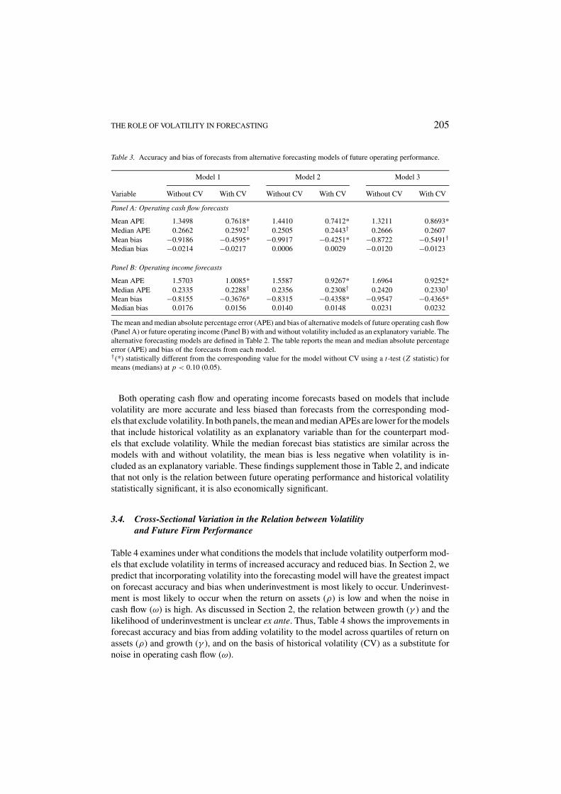
Table 3. Accuracy and bias of forecasts from alternative forecasting models of future operating performance.

Model 1 Model 2 Model 3

Variable Without CV With CV Without CV With CV Without CV With CV

Panel A: Operating cash flow forecasts

Mean APE 1.3498 0.7618* 1.4410 0.7412* 1.3211 0.8693*Median APE 0.2662 0.2592† 0.2505 0.2443† 0.2666 0.2607Mean bias −0.9186 −0.4595* −0.9917 −0.4251* −0.8722 −0.5491†

Median bias −0.0214 −0.0217 0.0006 0.0029 −0.0120 −0.0123

Panel B: Operating income forecasts

Mean APE 1.5703 1.0085* 1.5587 0.9267* 1.6964 0.9252*Median APE 0.2335 0.2288† 0.2356 0.2308† 0.2420 0.2330†

Mean bias −0.8155 −0.3676* −0.8315 −0.4358* −0.9547 −0.4365*Median bias 0.0176 0.0156 0.0140 0.0148 0.0231 0.0232

The mean and median absolute percentage error (APE) and bias of alternative models of future operating cash flow(Panel A) or future operating income (Panel B) with and without volatility included as an explanatory variable. Thealternative forecasting models are defined in Table 2. The table reports the mean and median absolute percentageerror (APE) and bias of the forecasts from each model.†(*) statistically different from the corresponding value for the model without CV using a t-test (Z statistic) formeans (medians) at p < 0.10 (0.05).

Both operating cash flow and operating income forecasts based on models that includevolatility are more accurate and less biased than forecasts from the corresponding mod-els that exclude volatility. In both panels, the mean and median APEs are lower for the modelsthat include historical volatility as an explanatory variable than for the counterpart mod-els that exclude volatility. While the median forecast bias statistics are similar across themodels with and without volatility, the mean bias is less negative when volatility is in-cluded as an explanatory variable. These findings supplement those in Table 2, and indicatethat not only is the relation between future operating performance and historical volatilitystatistically significant, it is also economically significant.

3.4. Cross-Sectional Variation in the Relation between Volatilityand Future Firm Performance

Table 4 examines under what conditions the models that include volatility outperform mod-els that exclude volatility in terms of increased accuracy and reduced bias. In Section 2, wepredict that incorporating volatility into the forecasting model will have the greatest impacton forecast accuracy and bias when underinvestment is most likely to occur. Underinvest-ment is most likely to occur when the return on assets (ρ) is low and when the noise incash flow (ω) is high. As discussed in Section 2, the relation between growth (γ ) and thelikelihood of underinvestment is unclear ex ante. Thus, Table 4 shows the improvements inforecast accuracy and bias from adding volatility to the model across quartiles of return onassets (ρ) and growth (γ ), and on the basis of historical volatility (CV) as a substitute fornoise in operating cash flow (ω).


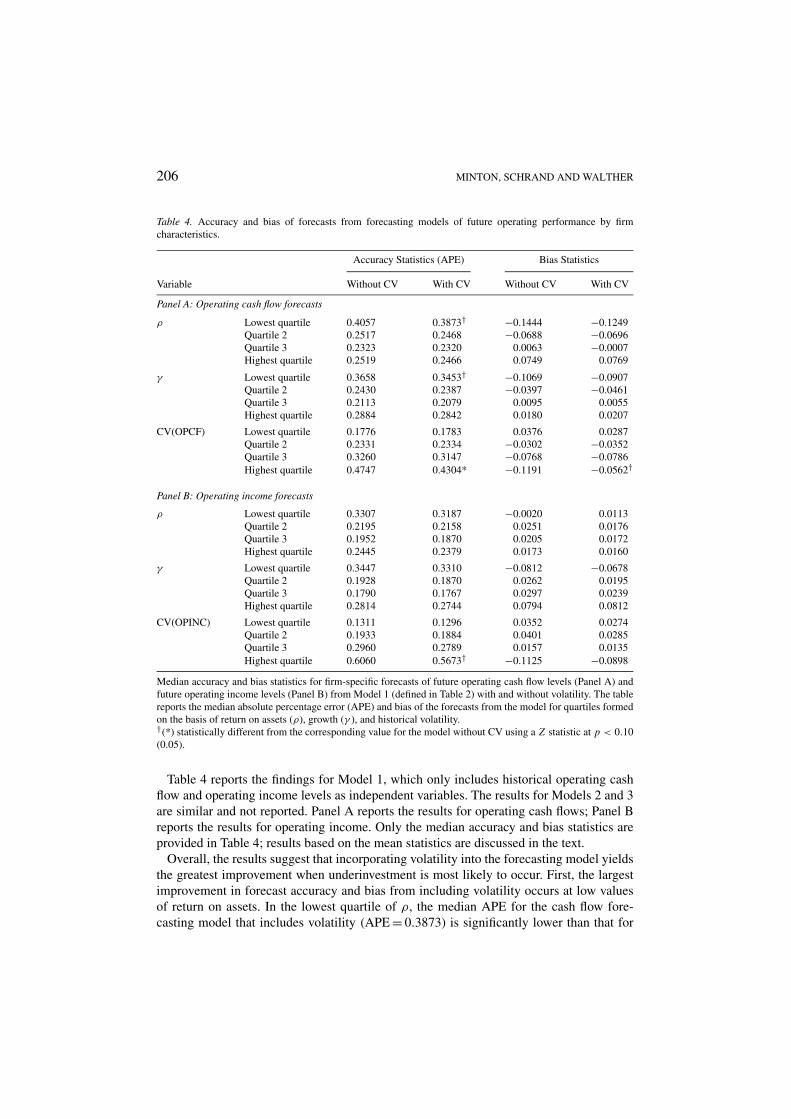
Table 4. Accuracy and bias of forecasts from forecasting models of future operating performance by firmcharacteristics.

Accuracy Statistics (APE) Bias Statistics

Variable Without CV With CV Without CV With CV


ρ Lowest quartile 0.4057 0.3873† −0.1444 −0.1249Quartile 2 0.2517 0.2468 −0.0688 −0.0696Quartile 3 0.2323 0.2320 0.0063 −0.0007Highest quartile 0.2519 0.2466 0.0749 0.0769

γ Lowest quartile 0.3658 0.3453† −0.1069 −0.0907Quartile 2 0.2430 0.2387 −0.0397 −0.0461Quartile 3 0.2113 0.2079 0.0095 0.0055Highest quartile 0.2884 0.2842 0.0180 0.0207

CV(OPCF) Lowest quartile 0.1776 0.1783 0.0376 0.0287Quartile 2 0.2331 0.2334 −0.0302 −0.0352Quartile 3 0.3260 0.3147 −0.0768 −0.0786Highest quartile 0.4747 0.4304* −0.1191 −0.0562†


ρ Lowest quartile 0.3307 0.3187 −0.0020 0.0113Quartile 2 0.2195 0.2158 0.0251 0.0176Quartile 3 0.1952 0.1870 0.0205 0.0172Highest quartile 0.2445 0.2379 0.0173 0.0160

γ Lowest quartile 0.3447 0.3310 −0.0812 −0.0678Quartile 2 0.1928 0.1870 0.0262 0.0195Quartile 3 0.1790 0.1767 0.0297 0.0239Highest quartile 0.2814 0.2744 0.0794 0.0812

CV(OPINC) Lowest quartile 0.1311 0.1296 0.0352 0.0274Quartile 2 0.1933 0.1884 0.0401 0.0285Quartile 3 0.2960 0.2789 0.0157 0.0135Highest quartile 0.6060 0.5673† −0.1125 −0.0898

Median accuracy and bias statistics for firm-specific forecasts of future operating cash flow levels (Panel A) andfuture operating income levels (Panel B) from Model 1 (defined in Table 2) with and without volatility. The tablereports the median absolute percentage error (APE) and bias of the forecasts from the model for quartiles formedon the basis of return on assets (ρ), growth (γ ), and historical volatility.†(*) statistically different from the corresponding value for the model without CV using a Z statistic at p < 0.10(0.05).

Table 4 reports the findings for Model 1, which only includes historical operating cashflow and operating income levels as independent variables. The results for Models 2 and 3are similar and not reported. Panel A reports the results for operating cash flows; Panel Breports the results for operating income. Only the median accuracy and bias statistics areprovided in Table 4; results based on the mean statistics are discussed in the text.

Overall, the results suggest that incorporating volatility into the forecasting model yieldsthe greatest improvement when underinvestment is most likely to occur. First, the largestimprovement in forecast accuracy and bias from including volatility occurs at low valuesof return on assets. In the lowest quartile of ρ, the median APE for the cash flow fore-casting model that includes volatility (APE = 0.3873) is significantly lower than that for


the cash flow forecasting model that excludes volatility (APE = 0.4057, Panel A). In thissubsample, the mean APE is also significantly lower when volatility is included in the cashflow forecasting model (APE = 0.9597) than when it is not (APE = 1.6536, not tabulated).While the median APE and bias are not significantly different in Panel B, the mean APEis significantly lower (1.7198 versus 1.0185) and the mean bias is significantly closer tozero (−0.9883 versus −0.3712) at p < 0.05 for the operating income model that includesvolatility (not tabulated). At lower levels of return (ρ), a firm is more likely to be forcedto forgo investment because of lower cash levels. Thus, the results support the hypothesisthat incorporating volatility into the forecast model improves the relative accuracy and biaswhen underinvestment is most likely to occur.

Second, the results suggest that incorporating volatility into the forecasting model im-proves forecasts the most for firms experiencing low growth. Panel A reports that for thelowest quartile of γ , the mean and median APE are significantly lower for the cash flowforecasting model that includes volatility. While the reported median bias statistics are notsignificantly different in Panel A, the mean bias is significantly less negative (−1.9063versus −0.8434, not tabulated) when volatility is included in the cash flow forecastingmodel.

While the median APE statistics are not significantly different in Panel B, the mean APEfor the operating income model with volatility (1.2870) is significantly lower than the meanAPE without volatility (2.3336, p < 0.05) for the lowest quartile of γ . Further, the mean biasstatistic is significantly improved from incorporating volatility into the operating incomemodel for firms with the lowest level of growth (−1.7484 versus −0.7627, not tabulated).Overall, these results suggest that the improvement from incorporating volatility is greatestat low levels of growth.

Finally, forecast accuracy is most improved from incorporating volatility into the modelfor firms with volatility in the highest quartile. For both operating cash flow and operatingincome forecasts, the mean and median APEs for the model that excludes volatility aresignificantly greater than the mean and median APEs for the model that includes volatilityin the highest quartile of CV.

Forecast bias also is most improved in the highest quartile of CV. The median bias statisticin Panel A for the cash flow forecasting model without volatility is −0.1191, compared to−0.0562 for the model with volatility (p < 0.10). While the median bias is improved inPanel B as well, only the mean bias is significantly different for the highest quartile ofCV(OPINC) (−1.7192 versus −0.5955, p < 0.10, results not tabulated).

As discussed in Section 2, a firm is more likely to experience underinvestment at higherlevels of cash flow volatility. Therefore, these findings support the conclusion that volatilityimproves the relative accuracy of the forecasting models when underinvestment, and thusa lumpy investment pattern, is likely to occur.

4. Valuation Implications

The results of the previous section indicate a role for volatility in forecasting, especially incases when underinvestment is most likely to occur. In this section, we test whether investorsincorporate information about volatility in their estimates of future firm performance. Prior


research suggests that individuals have difficulty incorporating information about varianceinto their decisions and judgments (see Ashton, 1982, pp. 101–108 for a summary of thefindings). We examine the profitability of trading strategies that assume market participantsdo not incorporate volatility into forecasts of future operating cash flows and future operatingincome. In Section 4.2, we investigate the relation between our findings and other previouslydocumented anomalies.

4.1. Trading Strategies Based on Historical Volatility

We implement a trading strategy that assumes investors ignore the information in volatilityin setting prices. We forecast one-year ahead operating performance levels for each firmusing specifications of the forecasting models that include and exclude volatility. We buy(sell) firms for which the forecast from the model that includes volatility is greater (less)than the forecast from the same model without volatility, and calculate excess returns forthe portfolio. We implement this trading strategy for both forecasts of future operating cashflows and future operating income, and for all three forecasting models.

Size-adjusted portfolio excess returns in year t + 1 are measured over two windows. Theannual window begins four months after the firm’s fiscal year-end of the year in whichwe measure the level of earnings, level of cash flow, level of investment, and historicalvolatility. The second window is the sum of the three-day excess return around each of thefour quarterly earnings announcement dates in year t + 1. The size-adjusted excess returnfor each sample observation is the firm’s raw buy-hold return minus the buy-hold return ona size-matched, value-weighted portfolio of firms based on market value of equity decilesof NYSE, AMEX, and NASDAQ firms from CRSP.

The significant hedge returns in Panel A of Table 5 suggest that investors do not considerthe information in historical cash flow volatility when forecasting future operating cashflow, despite greater accuracy and lower bias from the models that include volatility. Thetrading strategy returns over the annual window range from 2.88% for Model 1 to 5.86%for Model 3. All are significantly different from zero with the exception of the mean returnfor Model 1.

All trading strategy returns over the earnings announcement date window also are statis-tically significant at p < 0.10, and range from 1.85% for Model 1 to 2.91% for Model 3.Thus, regardless of the underlying model we assume investors use to forecast cash flows,the results suggest that investors do not incorporate the information in historical cash flowvolatility in price, even though it has value for predicting future cash flow performance andthus returns.

This conclusion holds if we instead assume that investors predict earnings and value theearnings predictions to set a price. In Panel B, we recompute the trading strategy resultsusing forecasting models that predict future operating income rather than cash flows.10

The mean and median hedge returns for the annual window are positive and significant forModels 1 and 3. The mean and median hedge returns around the earnings announcementdate range from 2.05% to 3.26%, and are significantly positive regardless of the forecastingmodel examined. These findings again suggest that investors do not fully incorporate theinformation in volatility for future firm performance.


Table 5. Trading strategy returns based on predicted operating performance.

Earnings AnnouncementAnnual Returns Date Returns

Portfolio Mean Median Mean Median


Model 1: With v. without CVLong 1.04% −0.26% 2.79% 2.32%Short −1.84 −4.11 0.71 0.47Hedge return 2.88 3.85† 2.08† 1.85*

Model 2: With v. without CVLong 1.90% 0.49% 2.89% 2.73%Short −2.34 −4.27 0.87 0.37Hedge return 4.24* 4.76* 2.02† 2.36*

Model 3: With v. without CVLong 1.72% 0.83% 2.91% 3.28%Short −2.27 −5.03 0.63% 0.37Hedge return 3.99† 5.86* 2.28* 2.91*


Model 1: With v. without CVLong 2.28% 0.37% 2.42% 2.95%Short −0.47 −2.26 0.30 0.08Hedge return 2.75† 2.63* 2.12* 2.87*

Model 2: With v. without CVLong 1.12% 0.34% 2.59% 3.45%Short 0.87 −0.27 0.54 0.92Hedge return 0.25 0.61 2.05* 2.53†

Model 3: With v. without CVLong 1.81% 0.29% 2.60% 2.93%Short −2.75 −1.45 0.11% −0.33Hedge return 4.56* 1.74* 2.49* 3.26*

Excess returns to trading strategies that use forecasting models that include volatility as an independent variableinstead of forecasting models that exclude volatility. Table 2 provides the forecasting models. In Panel A, a long(short) position is taken in firms for which the forecasted cash flow level for t + 1 from the model with volatilityis greater (less) than the forecasted cash flow level for t + 1 from the model without volatility. In Panel B, a long(short) position is taken in firms for which the forecasted operating income level for t + 1 from the model withvolatility is greater (less) than the forecasted operating income level for t + 1 from the model without volatility.The annual abnormal return to each portfolio is the mean one-year size-adjusted excess return beginning fourmonths after the fiscal year-end. The earnings announcement date abnormal return is the sum of the mean three-day size-adjusted excess return around the four earnings announcements for t + 1.†(*) statistically different from zero using a t-test (Z statistic) for means (medians) at p < 0.10 (0.05).

Our results are closely related to the previously documented “predictability bias” in stockreturns. Huberts and Fuller (1995) document that firms with the least predictable earningsper share have the greatest positive analyst forecast errors and related negative abnormalreturns (see also Weary, 1998). The lower than expected earnings for firms with high earningsvolatility is consistent with analysts ignoring the impact of volatility on the likelihood ofunderinvestment and thus future cash flows and future earnings. The negative abnormal


returns are consistent with our evidence that investors also fail to incorporate in prices theinformation in historical volatility.

4.2. Relation of Our Results with Other Trading Strategies

In this section, we relate our findings to Sloan’s (1996) profitable trading strategy and asubsequent examination of his results by Ali, Hwang and Trombley (2000). Sloan (1996)documents an abnormal return of approximately 11% from a trading strategy that takes along position in firms with low earnings but high cash flow and a short position in firmswith high earnings but low cash flow.11 The profitability of this trading strategy suggeststhat investors ignore information in cash flow for future firm performance.

We predict that the accuracy of models of future operating cash flow that exclude volatilityas an explanatory variable is greatest when historical cash flow volatility is low, and theempirical analysis supports this prediction. If investors also ignore the effect of historicalvolatility on the relation between historical and future measures, then the profitability ofSloan’s (1996) trading strategy will be greatest when cash flow volatility is low and thushistorical cash flow is most relevant for future cash flow.

We analyze the returns to Sloan’s (1996) trading strategy conditioning on historical cashflow volatility. For each sample year, we separate firms into quintiles based on historicalaccruals and historical cash flow volatility, resulting in 25 portfolios.12 We take a longposition in low-volatility firms that have low accruals and a short position in low-volatilityfirms that have high accruals (i.e., high earnings but low cash flow). While we expect thatthe strategy will be more profitable for low-volatility firms, we implement the same strategywith respect to accruals for high-volatility firms as a benchmark. Following Sloan (1996),we examine the size-adjusted excess annual return beginning four months after the firm’sfiscal year-end of the year in which the level of earnings, level of cash flow, and historicalcash flow volatility are measured.

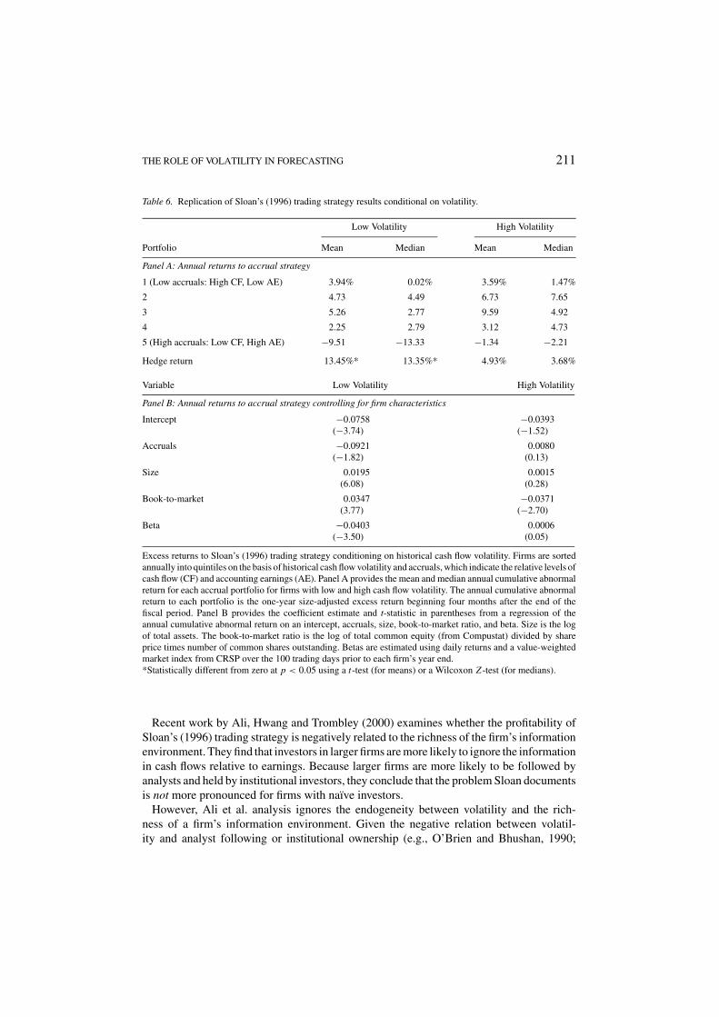
Panel A of Table 6 provides the mean and median excess returns for each accrual portfolio,separately for firms with low and high cash flow volatility. For firms with low cash flowvolatility, the average annual size-adjusted excess return to the long position is +3.94%and the return to the short position is −9.51%, for a hedge return of +13.45% (t =2.37, p < 0.04, Panel A).13 The hedge return is positive in 15 of 18 years. By contrast, theaverage annual hedge return for the high-volatility firms is insignificantly different fromzero (4.93%, t = 1.01, p > 0.10).

To ensure that the difference in hedge returns between low and high volatility firms is notattributable to an omitted risk factor, Panel B of Table 6 regresses the annual size-adjustedexcess return on firm characteristics (see Sloan, 1996).14 The characteristics considered aresize (measured as the logarithm of total assets), book-to-market (measured as the log of theratio of the book value of equity to the market value of equity), and firm beta (measured byestimating the market model on the prior 100 trading days). Consistent with the findings inPanel A, the estimated coefficient on accruals is significant only for the low volatility firms.Replacing the continuous measure of accruals with a variable that represents the accrualportfolio rank yields similar results (not tabulated). Thus, the ability of accruals to predictfuture returns for low volatility firms but not high volatility firms is not due to differencesin risk characteristics.


Table 6. Replication of Sloan’s (1996) trading strategy results conditional on volatility.

Low Volatility High Volatility

Portfolio Mean Median Mean Median

Panel A: Annual returns to accrual strategy

1 (Low accruals: High CF, Low AE) 3.94% 0.02% 3.59% 1.47%

2 4.73 4.49 6.73 7.65

3 5.26 2.77 9.59 4.92

4 2.25 2.79 3.12 4.73

5 (High accruals: Low CF, High AE) −9.51 −13.33 −1.34 −2.21

Hedge return 13.45%* 13.35%* 4.93% 3.68%

Variable Low Volatility High Volatility

Panel B: Annual returns to accrual strategy controlling for firm characteristics

Intercept −0.0758 −0.0393(−3.74) (−1.52)

Accruals −0.0921 0.0080(−1.82) (0.13)

Size 0.0195 0.0015(6.08) (0.28)

Book-to-market 0.0347 −0.0371(3.77) (−2.70)

Beta −0.0403 0.0006(−3.50) (0.05)

Excess returns to Sloan’s (1996) trading strategy conditioning on historical cash flow volatility. Firms are sortedannually into quintiles on the basis of historical cash flow volatility and accruals, which indicate the relative levels ofcash flow (CF) and accounting earnings (AE). Panel A provides the mean and median annual cumulative abnormalreturn for each accrual portfolio for firms with low and high cash flow volatility. The annual cumulative abnormalreturn to each portfolio is the one-year size-adjusted excess return beginning four months after the end of thefiscal period. Panel B provides the coefficient estimate and t-statistic in parentheses from a regression of theannual cumulative abnormal return on an intercept, accruals, size, book-to-market ratio, and beta. Size is the logof total assets. The book-to-market ratio is the log of total common equity (from Compustat) divided by shareprice times number of common shares outstanding. Betas are estimated using daily returns and a value-weightedmarket index from CRSP over the 100 trading days prior to each firm’s year end.*Statistically different from zero at p < 0.05 using a t-test (for means) or a Wilcoxon Z -test (for medians).

Recent work by Ali, Hwang and Trombley (2000) examines whether the profitability ofSloan’s (1996) trading strategy is negatively related to the richness of the firm’s informationenvironment. They find that investors in larger firms are more likely to ignore the informationin cash flows relative to earnings. Because larger firms are more likely to be followed byanalysts and held by institutional investors, they conclude that the problem Sloan documentsis not more pronounced for firms with naıve investors.

However, Ali et al. analysis ignores the endogeneity between volatility and the rich-ness of a firm’s information environment. Given the negative relation between volatil-ity and analyst following or institutional ownership (e.g., O’Brien and Bhushan, 1990;


Minton and Schrand, 1999), firms with richer information sets also are more likely to havelower cash flow volatility. Therefore, a more intuitive and economically appealing expla-nation for the greater abnormal returns for large firms found by Ali, Hwang and Trombley(2000) is that historical cash flows are better predictors of future cash flow levels for thesefirms.

5. Conclusions

This paper links results from the risk management literature that show a relation betweenvolatility, investment, and firm value to the literature on forecasting. When current periodinvestment decisions are a function of current period cash flow realizations, a firm’s invest-ment pattern through time depends on cash flow volatility. Thus, volatility will affect futurecash flows and future income levels. As a result, we predict that volatility has explanatorypower for future operating performance incremental to that in historical cash flow, earn-ings, investment, or other firm characteristics related to the cash flow generation process(such as return on assets and growth). Further, we predict that incorporating volatility into aforecasting model improves forecast accuracy and bias most when volatility causes periodsof underinvestment and thus a lumpy investment pattern. Lumpy investment is most likelyto occur when return on assets is low and noise in cash flow is high.

Four main results emerge from our empirical analysis. First, consistent with our pre-dictions, volatility has incremental explanatory power for future operating cash flows andoperating income beyond traditional forecasting models. Second, forecasting models thatincorporate volatility provide more accurate and less biased forecasts than correspondingmodels that exclude volatility as an explanatory variable. Third, the relative improvementsfrom incorporating volatility are greater when underinvestment is most likely to occur.Finally, the profitability of a trading strategy that relies on the first three findings suggeststhat investors do not fully incorporate information on volatility in equity valuation. Theresults from our empirical analyses can be used to improve existing forecasts of cash flowand earnings levels in equity valuation as well as in other contexts.

Acknowledgments

The authors appreciate comments from Mary Barth, Ted Goodman, Adam Koch, LisaKoonce, Rick Lambert, James Livingston, Doron Nissim, Richard Sloan, Rene Stulz,Ro Verrecchia, Karen Wruck, two anonymous reviewers, and seminar participants at Amer-ican Accounting Association 2000 annual meetings, Australian Graduate School of Man-agement, Baruch College, Carnegie-Mellon, University of Chicago, Columbia Univer-sity’s Burton Workshop, Duke University/University of North Carolina’s fall camp, EmoryUniversity, Georgetown University, University of Illinois, University of Melbourne, Univer-sity of Minnesota’s mini-conference, New York University, Review of Accounting Studies2001 conference, and University of Texas, and the computer assistance of Jim Noonan.Minton thanks the Dice Center for Financial Economics for financial support. Waltherthanks the Accounting Research Center at the Kellogg School of Management for financialsupport.


Notes

1. Prior work also has documented a positive association between liquidity and investment levels (e.g., Fazzari,Hubbard and Peterson, 1988, 1998; Hoshi, Kashyap and Scharfstein, 1991; Kaplan and Zingales, 1997; Lamont,1997). Unlike Minton and Schrand (1999), these results indicate that firms time investments to match cash flowlevels but do not necessarily imply that firms forgo investments when cash flow realizations are low. Lumpyinvestment also can be a rational choice because of the real options embedded in certain investment projects,such as when to invest, whether to abandon a project, or whether to modify a product midstream (e.g., Berger,Ofek and Swary, 1996; Dixit and Pindyck, 1993; Majd and Pindyck, 1987; Pindyck, 1988; Trigeorgis, 1996).

2. The predictions were originally based on a model of a firm’s cash flow generation process that incorporatedunderinvestment. A detailed description of the model and the simulation analysis used to develop the predictionsis provided in Minton, Schrand and Walther (2001).

3. The adjustment for working capital accruals subtracts the changes in accounts receivable, inventory, and othercurrent assets, and adds back the changes in accounts payable and other current liabilities.

4. We estimate quarterly advertising expense since these Compustat data are available only on an annual basis.Quarterly research and development data are available from Compustat beginning in the first quarter of 1989.The mean of the actual quarterly amount for all firms on Compustat from 1989 to 1997 is virtually identicalto that of our estimated amount ($7.03 million versus $7.05 million), and the Pearson (Spearman) correlationbetween these two numbers is 0.96 (0.99).

5. The results in Sections 3.2 through 3.4 are qualitatively similar if we calculate operating cash flow using operat-ing income before depreciation (defined as net sales minus cost of goods sold minus selling and administrativeexpenses) adjusted for the change in accruals, and/or if we do not adjust the operating cash flow number forresearch and development or advertising expenses. The results also are insensitive to alternative definitions ofoperating income, including net income or net income before extraordinary items and discontinued operations.

6. In the tabulated results, we eliminate observations with studentized residuals greater than two in absolute valueor Cook’s D greater than one; the results are not sensitive to this outlier elimination.

7. To provide additional evidence on the underinvestment story, we examine the relation between historical cashflow volatility and future investment levels, after controlling for historical operating cash flow and operatingincome levels. As expected, the mean estimated coefficient on CV(OPCF) in this specification is negativeand statistically significant (−0.0017, Z ′ = − 2.910, p < 0.01). Thus, higher levels of cash flow volatility areassociated with lower levels of future investment, consistent with Minton and Schrand (1999).

8. The results are robust to alternative measures of quarterly capital expenditures, including the amount reportedby Compustat (available the first quarter of 1984) or annual capital expenditures from 10-K Schedule V dividedby four, and to the exclusion of research and development and advertising expenses from the definition ofinvestment.

9. Using the mean of the coefficients from the prior three or five yearly regressions result in more accurate andless biased forecasts, but does not change any of our inferences.

10. We also computed the hedge returns from taking a long (short) position in firms for which both the cash flowforecast and the earnings forecast from the model that includes volatility are greater than the cash flow andearnings forecasts, respectively, from the same model that excludes volatility. All inferences are unchanged.

11. In our sample, the average hedge return to Sloan’s (1996) strategy is 10.76% when we divide observationsinto separate deciles for historical cash flow and historical earnings levels. We use quintiles for the remainderof the tests due to the small sample size in each combination of decile classifications. Implementing Sloan’sstrategy for quintiles is lower but still positive (8.76%).

12. The minimum number of observations per portfolio is five in 1993, the maximum is 53 in 1989, and the averageover all years is 23.7. Our conclusions are unchanged if we segregate sample firms into portfolios based onhistorical cash flow and earnings levels.

13. There are also significant excess returns to a trading strategy that relies only on historical cash flow volatilityand historical cash flow levels and ignores earnings. The average annual hedge return for a strategy that takesa long position in firms with high cash flow levels and low volatility (+7.33%) and a short position in firmswith low cash flow levels and low volatility (−6.14%) is +13.47%.

14. As an alternative means of assessing whether our findings are due to differences in risk, we implemented atrading strategy based solely on historical volatility. This trading strategy takes a long (short) position in firmsin the lowest (highest) quintile of historical volatility. Regardless of whether we form the quintiles on the basis


of CV(OPCF) or CV(OPINC), the mean and median hedge returns over the annual window are insignificantlydifferent from zero.

References

Abarbanell, J. S. and B. J. Bushee. (1997). “Fundamental Analysis, Future Earnings, and Stock Prices.” Journalof Accounting Research 35, 1–24.

Abarbanell, J. S. and B. J. Bushee. (1998). “Abnormal Returns to a Fundamental Analysis Strategy.” The AccountingReview 73, 19–45.

Albrecht, W. D. and F. M. Richardson. (1990). “Income Smoothing by Economy Sector.” Journal of Business,Finance and Accounting 17, 713–730.

Alford, A. W. and P. G. Berger. (1999). “A Simultaneous Equations Analysis of Forecast Accuracy, AnalystFollowing, and Trading Volume.” Journal of Accounting, Auditing and Finance 14, 219–240.

Ali, A., L.-S. Hwang and M. A. Trombley. (2000). “Accruals and Future Stock Returns: Tests of the Naive InvestorHypothesis.” Journal of Accounting, Auditing and Finance 15, 161–181.

Amihud, Y. and H. Mendelson. (1988). “Liquidity and Asset Prices: Financial Management Implications.”Financial Management 7, 5–15.

Ashton, R. H. (1982). Human Information Processing in Accounting, American Accounting Association,Sarasota, FL.

Barth, M. E., D. P. Cram and K. K. Nelson. (2001). “Accruals and the Prediction of Future Cash Flows.” TheAccounting Review 76, 27–58.

Beaver, W., P. Kettler and M. Scholes. (1970). “The Association between Market Determined and AccountingDetermined Risk Measures.” The Accounting Review 45, 654–682.

Berger, P. G., E. Ofek and I. Swary. (1996). “Investor Valuation of the Abandonment Option.” Journal of FinancialEconomics 42, 257–287.

Bernard, V. L. and T. L. Stober. (1989). “The Nature and Amount of Information in Cash Flows and Accruals.”The Accounting Review 64, 624–652.

Bowen, R. M., D. Burgstahler and L. A. Daley. (1986). “Evidence on the Relationships between Earnings andVarious Measures of Cash Flow.” The Accounting Review 61, 713–725.

Dechow, P. M. (1994). “Accounting Earnings and Cash Flows as Measures of Firm Performance: The Role ofAccounting Accruals.” Journal of Accounting and Economics 18, 3–42.

Dixit, A. K. and R. S. Pindyck. (1993). Investment Under Uncertainty, Princeton, NJ: Princeton Press.Fazzari, S. M., R. G. Hubbard and B. C. Petersen. (1988). “Financing Constraints and Corporate Investment.”

Brookings Papers on Economic Activity, 141–195.Fazzari, S. M., R. G. Hubbard and B. C. Petersen. (1998). “Investment-Cash Flow Sensitivities are Useful: A

Comment on Kaplan and Zingales.” Working Paper, Columbia University.Finger, C. (1994). “The Ability of Earnings to Predict Future Earnings and Cash Flow.” Journal of Accounting

Research 32, 210–223.Francis, J., P. Olsson and D. R. Oswald. (2000). “Comparing the Accuracy and Explainability of Dividend, Free

Cash Flow, and Abnormal Earnings Equity Value Estimates.” Journal of Accounting Research 38, 45–70.Froot, K., D. Scharfstein and J. Stein. (1993). “Risk Management: Coordinating Investment and Financing

Policies.” Journal of Finance 48, 1629–1658.Gebhardt, W. R., C. M. C. Lee and B. Swaminathan. (2001). “Toward an Implied Cost of Capital.” Journal of

Accounting Research 39, 135–176.Geczy, C., B. A. Minton and C. Schrand. (1997). “Why Firms Use Currency Derivatives.” Journal of Finance 52,

1323–1354.Graham, J. and C. Smith. (1999). “Tax Incentives to Hedge.” Journal of Finance 54, 2241–2262.Guay, W. (1999). “The Impact of Derivatives on Firm Risk: An Empirical Examination of New Derivative Users.”

Journal of Accounting and Economics 26, 319–351.Hoshi, T., A. Kashyap and D. Scharfstein. (1991). “Corporate Structure, Liquidity, and Investment: Evidence from

Japanese Industrial Groupings.” Quarterly Journal of Economics 56, 33–60.Huberts, L. C. and R. J. Fuller. (1995). “Predictability Bias in the U.S. Equity Market.” Financial Analysts Journal

51, 12–28.Kaplan, S. N. and L. Zingales. (1997). “Do Investment-Cash Flow Sensitivities Provide Useful Measures of

Financing Constraints?” Quarterly Journal of Economics 112, 169–215.


Lamont, O. (1997). “Cash Flow and Investment: Evidence from Internal Capital Markets.” Journal of Finance 52,83–111.

Lev, B. and S. R. Thiagarajan. (1993). “Fundamental Information Analysis.” Journal of Accounting Research 31,190–215.

Lim, T. (2001). “Rationality and Analysts’ Forecasts Bias.” Journal of Finance 61, 369–385.Majd, S. and R. S. Pindyck. (1987). “Time to Build, Option Value and Investment Decisions.” Journal of Financial

Economics 18, 7–27.Mian, S. L. (1996). “Evidence on Corporate Hedging Policy.” Journal of Financial and Quantitative Analysis 31,

419–439.Michelson, S. E., J. Jordan-Wagner and C. W. Wootton. (1995). “A Market Based Analysis of Income Smoothing.”

Journal of Business, Finance and Accounting 22, 1179–1193.Minton, B. and C. Schrand. (1999). “The Impact of Cash Flow Volatility on Discretionary Investment and the

Costs of Debt and Equity Financing.” Journal of Financial Economics 54, 423–460.Minton, B., C. Schrand and B. Walther. (2001). “Forecasting Cash Flow for Valuation: Is Cash Flow Volatility

Informative?” Working Paper, Ohio State University.Myers, S. C. (1977). “Determinants of Corporate Borrowing.” Journal of Financial Economics 5, 147–175.Nance, D. R., C. W. Smith, Jr. and C. W. Smithson. (1993). “On the Determinants of Corporate Hedging.” Journal

of Finance 48, 267–284.O’Brien, P. C. and R. Bhushan. (1990). “Analyst Following and Institutional Ownership.” Journal of Accounting

Research 28, 55–76.Pindyck, R. S. (1988). “Irreversible Investment, Capacity Choice, and the Value of the Firm.” American Economic

Review 78, 969–985.Shapiro, A. and S. Titman. (1986). “An Integrated Approach to Corporate Risk Management.” In: J. Stern and

D. Chew (eds.), The Revolution in Corporate Finance. England: Basil Blackwell Ltd, Cambridge, MA: BasilBlackwell, Inc.

Sloan, R. (1996). “Using Earnings and Free Cash Flow to Evaluate Corporate Performance.” Journal of AppliedCorporate Finance, 70–78.

Smith, C. W. and R. M. Stulz. (1985). “The Determinants of Firms’ Hedging Policies.” Journal of Financial andQuantitative Analysis 20, 391–405.

Trigeorgis, L. (1996). Real Options: Managerial Flexibility and Strategy in Resource Allocation. Cambridge, MA:MIT Press.

Walther, B. R. and R. H. Willis. (1999). “Are Earnings Surprises Costly?” Working Paper, Northwestern University.Waymire, G. (1985). “Earnings Volatility and Voluntary Management Forecast Disclosure.” Journal of Accounting

Research 23, 268–295.Weary, T. M. (1998). “Steady as She Goes! Earnings Stability and Investment Performance.” Journal of Investing

7, 54–60.Wilson, G. P. (1987). “The Incremental Information Content of the Accrual and Funds Components of Earnings

after Controlling for Earnings.” The Accounting Review 62, 293–322.

the role of volatility in forecasting

Documents