forecasting realized gold volatility: is there a role of
TRANSCRIPT
Forecasting Realized Gold Volatility:Is there a Role of Geopolitical Risks?
Konstantinos Gkillasa, Rangan Guptab, Christian Pierdziochc
May 2019
Abstract
We use a quantile-regression heterogeneous autoregressive realized volatility (QR-HAR-RV) model to study whether geopolitical risks have predictive value in sample and out-of-sample for realized gold-returns volatility estimated from intradaily data. We consideroverall geopolitical risks along with a decomposition into actual risks (i.e., acts) and threats,and we control for overall the impact of economic policy uncertainty (EPU). We find that,after controlling for EPU, the components of geopolitical risks have predictive power forrealized volatility mainly at a longer forecast horizon when we account for the potentialasymmetry of the loss function a forecaster uses to evaluate forecasts.
Keywords: Gold-price returns; Realized volatility; Geopolitical risks; Forecasting
a Corresponding author. Department of Business Administration, University of Patras− Univer-sity Campus, Rio, P.O. Box 1391, 26500 Patras, Greece; Email address: [email protected].
b Department of Economics, University of Pretoria, Pretoria, 0002, South Africa; E-mail address:[email protected].
c Department of Economics, Helmut Schmidt University, Holstenhofweg 85, P.O.B. 700822,22008 Hamburg, Germany; Email address: [email protected].
1 Introduction
The role of gold as a “safe haven" is well-recognized. In other words, during periods of height-
ened risks in other financial markets (Baur and Lucey 2010, Baur and McDermott 2010, Re-
boredo 2013a, b, Agyei-Ampomah et al. 2014, Gürgün and Ünalmis 2014, Beckmann et al.
2015), general economic uncertainty (Bouoiyour et al. 2018, Beckmann et al. 2019), and geopo-
litical risks (Baur and Smales 2018), gold provides portfolio-diversification benefits. Naturally,
forecasting volatility of gold returns is of interest to investors in the pricing of related derivatives
as well as for devising hedging strategies. Understandably, there exists a large literature that
has aimed to forecast gold volatility (see, Pierdzioch et al. 2016, Fang et al. 2018 for detailed
literature reviews). In general, while earlier studies have primarily utilized a wide-variety of
models from the Generalized Autoregressive Conditional Heteroskedasticity (GARCH)-family,
more recent papers have also use mixed-frequency and boosting approaches to accommodate for
the role of a wide variety of information from macroeconomic and financial variables while also
controlling for model uncertainty.
Realizing that rich information contained in intraday data can produce more accurate estimates
and forecasts of daily volatility (for a detailed discussion in this regard, see Degiannakis and
Filis 2017), we aim to extend the existing literature by forecasting the realized volatility (RV)
of gold returns (derived based on 5 minute-interval intraday data), using a modified version
of the Heterogeneous Autoregressive (HAR) model developed by Corsi (2009). In particular,
we augment the basic HAR-RV model with information on geopolitical risks, over and above
macroeconomic uncertainty, for the daily period from 3rd December, 1997 to 2000 to 30th May,
2017. In addition, in order to study the entire conditional distribution of the volatility of gold
returns, rather than just its conditional mean, we use a quantile regression version of the HAR-
RV (QR-HAR-RV). To the best of our knowledge, this is the first paper to analyse the role of
geopolitical risks in forecasting the entire conditional distribution of realized volatility of the
gold market.1
1In this regard, it should be noted that, while the focus of Baur and Smales (2018) was primarily to analyze
1
The remainder of the paper is organized as follows: We describe in Section 2 the methods that
we use in our empirical analysis. We present our data in Section 3, summarize our empirical
results in Section 4, and conclude in Section 5.
2 Methods
Andersen et al. (2012) propose median realized variance (MRVt) as a jump-robust estimator of
integrated variance using intraday data:2
MRVt=π
6−4√
3+π
TT −2
T−1
∑i=2
med (|rt,i−1|, |rt,i|, |rt,i+1|)2, (1)
where rt,i = is the intraday return i within day t, and i = 1, ..,T denotes the number of intraday
observations within a day. We consider MRV as our measure of daily realized volatility in order
to attenuate the effect of market-microstructure noise and jumps on our results. MRV , as a jump-
robust estimator of realized volatility is significantly less biased in the presence of jumps in the
price process.
Corsi (2009) has proposed the HAR-RV model as a technique to model and forecast realized
volatility. The HAR-RV has become one of the most popular models in the literature on realized
volatility because, despite its simple structure, the HAR-RV model captures “stylized facts” of
long memory and multi-scaling behavior associated with volatility of financial markets. The
benchmark HAR-RV model, for h−days-ahead forecasting, is given by:
RVt+h=β0 +βd RVt +βw RVw,t +βm RVm,t + εt+h, (2)
where RVw,t denotes the average RV from day t−5 to day t−1, while RVm,t denotes the average
RV j from day t−22 to day t−1.
the impact of changes in geopolitical risks on gold returns, using an exponential GARCH (EGARCH) model, theycould not detect evidence of any in-sample impact of such risks on gold market volatility.
2Researchers commonly use the term volatility to denote the standard deviation of returns. Because there is notrisk of confusion, we use in this research the terms realized volatility and realized variance interchangeably.
2
We use the standard HAR-RV model as our benchmark model for predicting realized-volatility
and then add geopolitical risks (GPR) and economic policy uncertainty (EPU) in order to explore
whether these two economic variables have any incremental predictive information. Because
changes in GPR and EPU should capture that new information that are revealed to traders, we
use GPR and EPU in first-differences.3 In analogy to RV , we further consider there weekly and
monthly averages of these variables. We consider the following two extended HAR-RV models:
RV jt+h=β0 +βd RVt +βw RVw,t +βm RVm,t +θ EPUt +θw EPUt,m +θm EPUt,m + εt+h,
(3)
RV jt+h=β0 +βd RVt +βw RVw,t +βm RVm,t +θ GPRt +θw GPRt,m +θm GPRt,m + εt+h.
(4)
While the baseline HAR-RV model and its two extensions are estimated by the ordinary-least
squares technique, we also consider a quantile-regression variant of the model. The quantile-
regression variant of the HAR-RV model accounts for the possibility that the predictive value
of the predictors differs across the quantiles of the conditional distribution of RV . The quantile-
regression HAR-RV model is given by:
b̂q = argmin∑i
ρq(RV ji+h−Xibq), i = 1,2, ..., t, (5)
where ρq(u) denotes the check function, ρq = εt+h(q− 1(εt+h < 0), q denotes a quantile, and
1 denotes the indicator function. Furthermore, the vector bq denotes the now quantile specific
parameters of the HAR-RV models in Eqs. 2, 3, and 4, a hat denotes the estimates of these
parameters, and the matrix X denotes the predictors of the HAR-RV models. Variants of the
quantile-regression variant of the HAR-RV model have been studied in recent research by Hau-
gom et al. (2016) and Balcilar et al. (2017), Baur and Dimpfl (2019). For other recent quantile-
regressions-based research on several key aspects of gold-price fluctuations, see i.a. Baur (2013),
Dee et al. (2013), Ma and Patterson (2013), Zagaglia and Marzo (2013), and Pierdzioch et al.
(2015).
3In this regard we follow Baur and Smales (2018). However, unlike them, we use EPU instead of the ChicagoBoard Options Exchange’s Volatility Index (VIX), to prevent substantial losses in data.
3
In order to study out-of-sample predictability of RV , we consider a fixed-length daily rolling-
estimatin window. We vary the length of the estimation window between 1000 and 3000 ob-
servations. We use the Diebold and Mariano (1995) test to compare forecast accuracy of the
HAR-RV models with and without geopolitical risk as a predictor. The test results are computed
in the R programming environment (R Core Team 2017) based on the modified Diebold-Mariano
test proposed by Harvey, Leybourne and Newbold (1997), we report the p-values calculated using
the R package “forecast” (Hyndman 2017, Hyndman and Khandakar 2008). We study the rela-
tive forecast errors of the models to account for heteroskedasticity (e.g., Bollerslev and Ghysels
1996).
3 Data
We use intraday data on gold futures traded in NYMEX over a 24 hour trading day (pit and elec-
tronic) to construct the daily measure of realized volatility. The futures price data, in continuous
format, are obtained from www.disktrading.com and www.kibot.com. Close to expiration of
a contract, the position is rolled over to the next available contract, provided that activity has
increased. Daily returns are computed as the end of day (New York time) price difference (close
to close). In the case of intraday returns, 1-minute prices are obtained via last-tick interpolation
(if the price is not available at the 1-minute stamp, the previously available price is imputed).
5-minute returns are then computed by taking the log-differences of these prices and are then
used to compute the realized moments.
Besides the intraday data, we obtain daily data on the EPU of the United States (US),4 as devel-
oped by Baker et al. (2016) based on newspaper archives from Access World New’s NewsBank
service. The primary measure for this index is the number of articles that contain at least one
term from each of 3 sets of terms namely, economic or economy, uncertain or uncertainty, and
legislation or deficit or regulation or congress or federal reserve or white house.5
4We understand that gold is a global market, but due to the unavailability of a daily measure of worldwideuncertainty, and the prominent role of the U.S. in the global economy, we use the EPU for the U.S. as a proxy forworld uncertainty.
5The data is available for download from: http://policyuncertainty.com/us_monthly.html.
4
As far as our main predictor of interest, i.e., the GPR is concerned, it is based on on the work
of Caldara and Iacoviello (2018).6 Caldara and Iacoviello (2018) construct the GPR index by
counting the occurrence of words related to geopolitical tensions, derived from automated text-
searches in 11 leading national and international newspapers (The Boston Globe, Chicago Tri-
bune, The Daily Telegraph, Financial Times, The Globe and Mail, The Guardian, Los Angeles
Times, The New York Times, The Times, The Wall Street Journal, and The Washington Post).
They then calculate an index by counting, in each of the above-mentioned 11 newspapers, the
number of articles that contain the search terms7 related to geopolitical risks for every day. Based
on the search groups, Caldara and Iacoviello (2018) further disentangle the direct effect of ad-
verse geopolitical events from the effect of pure geopolitical risks by constructing two additional
indexes, i.e., the Geopolitical Threats index,8 and the Geopolitical Acts index9
Our analysis covers the daily period of 3rd December, 1997 to 2000 to 30th May, 2017, with
the start and end dates being purely contingent on the availability of the intraday data on gold
futures.
4 Empirical Findings
Figure 1 displays the results for the benchmark HAR-RV models that we estimate using the
ordniary-least-squares techniques. We present results for three different forecast horizons. Specif-
ically, we set h = 1,5,22 and, thus, study whether the model has predictive value for RV one-
day-ahead, five-days-ahead (that is, one week), and 22-days-ahead (that is, approximately one
6The data can be downloaded from: https://www2.bc.edu/matteo-iacoviello/gpr.htm.7The search identifies articles containing references to six groups of words: Group 1 includes words associated
with explicit mentions of geopolitical risk, as well as mentions of military-related tensions involving large regionsof the world and a U.S. involvement; Group 2 includes words directly related to nuclear tensions; Groups 3 and4 include mentions related to war threats and terrorist threats, respectively; Groups 5 and 6 aim at capturing presscoverage of actual adverse geopolitical events (as opposed to just risks) which can be reasonably expected to leadto increases in geopolitical uncertainty, such as terrorist acts or the beginning of a war.
8This index only includes words belonging to Search groups 1 to 4,9 This index only includes words belonging to Search groups 5 and 6.
5
month). We present results for a quadratic (L2) and a linear loss function (L1). Results show
that geopolitical risk improves forecast accuracy relative to the benchmark HAR-RV model, but
the results differ across model specifications. For L1 loss, we observe significant test results
mainly for the short and medium forecast horizon when we consider the HAR-RV model as our
benchmark. The test results for the long forecast horizon become significant once we opt for a
relatively long rolling-estimation window. When we consider the HAR-RV-EPU model as our
benchmark model, in contrast, we detect improvements in forecast accuracy for the medium and
long forecast horizons. Results for threats closely resemble those for geopolitical risks, while
the tests for actual realization of risk are only significant when we consider the HAR-RV-EPU
model as our benchmark model, and for relatively long rolling-estimation windows. When we
consider the L2 loss function, the results are by and large similar to the corresponding results
that we obtain for the L1 loss function.
− Please include Figure 1 about here. −
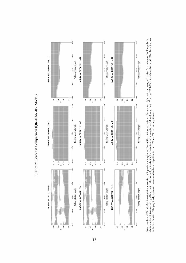
Figure 2 displays the results for the QR-HAR-RV model. For the quantile-regression-based
models, we use the check function to compare the forecast accuracy of (relative) forecast errors
(that is, a quasi-linear L1 loss function that, depending on the quantile parameter, is asymmetric
around zero). This choice of the loss function ensures that we evaluate forecsat errors by means
of the same loss function that we use to estimate the quantile-regression model. Results for the
short forecast horizon are significant mainyl for a range of quantiles between 0.2 and 0.4 and
between 0.6 and 0.8. FOr the medium forecast horizon, test results for all rolling-estimation
windows are significant, except for quantiles roughly smaller than 0.2 and larger than 0.8. For
the long forecast horizon, the test results are significant for quantiles larger than approximately
0.6, where the width of the area of significant test results depends varies somewhat across rolling-
estimation windows. Results are broadly similar for geoplitical risks, threats, and acts.
− Please include Figure 3 about here. −
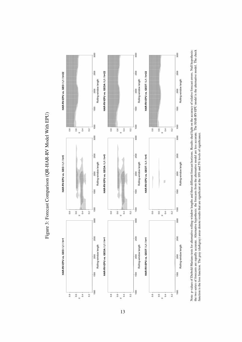
Figure 3 displays the results we obtain when we control for EPU. For the short forecast horizon,
results turn insignificant. For the medium forecast horizon, results (for geopolitical risks and
6
acts) remain significant for several rolling-estimation windows in the range of quantiles between
0.4 and 0.6 (when the rolling-estimation window is not too long). For the long forecast horizon,
in turn, the results are very similar to those we obtain when we use the HAR-RV model as our
benchmark model.
5 Concluding Remarks
In this paper, we examine the forecasting power of geopolitical risks (over and above eco-
nomic uncertainty) for the conditional distribution of gold returns volatility, using the quantiles-
regression version of the the popular heterogeneous autoregressive realized volatility (HAR-RV)
model. Our findings suggest that, after controlling for economy-wide uncertainty, the compo-
nents of geopolitical risk, i.e., threats and acts, have predictive power for realized volatility, but
mainly at a longer forecasting horizon when we account for the potential asymmetry of the loss
function a forecaster uses to evaluate forecasts. In sum, our results imply that using information
contained in geopolitical risks, investors can improve the design of optimal portfolios involving
gold to hedge against primarily long-run risks.
7
References
Agyei-Ampomah, S., Gounopoulos, D., and Mazouz, K. (2014). Does gold offer a better pro-
tection against sovereign debt crisis than other metals? Journal of Banking & Finance, 40,
507−521.
Baker, S., Bloom, N., and Davis, S. (2016). Measuring economic policy uncertainty. Quarterly
Journal of Economics, 131(4), 1593?1636.
Balcilar, M. Gupta, R., and Pierdzioch, C. (2017). On exchange-rate movements and gold-price
fluctuations: evidence for gold-producing countries from a nonparametric causality-in-
quantiles test. International Economics and Economic Policy, 14, 691−700.
Baur, D.G. (2013). The structure and degree of dependence: A quantile regression approach.
Journal of Banking and Finance, 37, 786−798.
Baur, D.G., and Dimpfl, T. (2019). Think again: volatility asymmetry and volatility persistence.
Studies in Nonlinear Dynamics & Econometrics, 23, 20170020.
Baur, D.G., and Lucey, B.M. (2010) Is gold a hedge or a safe haven? An analysis of stocks,
bonds and gold. The Financial Review, 45, 217−229.
Baur, D.G., and McDermott, T.K. (2010). Is gold a safe haven? International evidence. Journal
of Banking & Finance, 34, 1886−1898.
Baur, D.G., and Smales, L. (2018). Gold and geopolitical risk. Available at SSRN: https:
//ssrn.com/abstract=3109136.
Beckmann, J., Berger, T., and Czudaj, R. (2015) Does gold act a hedge or safe haven for stocks?
A smooth transition approach. Economic Modelling 48, 16−24
Beckmann, J., Berger, T., and Czudaj, R. (2019). Gold price dynamics and the role of uncer-
tainty. Quantitative Finance, 19, 663−681.
Bollerslev, T., and Ghysels, E. (1996). Periodic autoregressive conditional heteroscedasticity.
Journal of Business and Economics Statistics, 14, 139−151.
8
Bouoiyour, J., Selmi, R., and Wohar, M.E. (2018). Measuring the response of gold prices to
uncertainty: An analysis beyond the mean. Economic Modelling, 75(C), 105−116.
Caldara, D., and Iacoviello, M. (2018). Measuring Geopolitical Risk. Board of Governors of
the Federal Reserve System, International Finance Discussion Paper No. 1222.
Corsi, F. (2009). A simple approximate long-memory model of realized volatility. Journal of
Financial Economics, 7, 174−196.
Dee, J., Li, L., and Zheng, Z. (2013). Is gold a hedge or safe haven? Evidence from Inflation
and Stock Market. International Journal of Development and Sustainability, 2, 12−27.
Degiannakis, S., and Filis, G. (2017). Forecasting oil price realized volatility using information
channels from other asset classes. Journal of International Money and Finance, 76, 28−49.
Fang, L., Honghai, Y., and Xiao, W. (2018). Forecasting gold futures market volatility using
macroeconomic variables in the United States. Economic Modelling, 72, 249−259.
Gürgün, G. and Ünalmis, I. (2014) Is gold a safe haven against equity market investment in
emerging and developing countries? Finance Research Letters, 11, 341−348.
Haugom, E., Ray, R., Ulfrich, C.J., and Veka, S. (2016). A parsimonious quantile regression
model to forecast day-ahead value-at-risk. Finance Research Letters, 16, 196−207.
Ma, L., and Patterson, G. (2013). Is gold overpriced? Journal of Investing, 22, 113−127.
Pierdzioch, C., Risse, M., and Rohloff, S. (2015). A real-time quantile-regression approach to
forecasting gold-price fluctuations under asymmetric loss. Resources Policy, 45, 299−306.
Pierdzioch, C., Risse, M., and Rohloff, S. (2016). A boosting approach to forecasting the
volatility of gold-price fluctuations under flexible loss. Resources Policy, 47, 95−107.
Reboredo, J.C. (2013a). Is gold a safe haven or a hedge for the US dollar? Implications for risk
management. Journal of Banking & Finance, 37, 266−2676.
Reboredo, J.C. (2013b). Is gold a hedge or safe haven against oil price movements? Resources
Policy, 38, 130−137.
9
R Core Team (2017). R: A language and environment for statistical computing, Vienna, Austria:
R Foundation for Statistical Computing. URL http://www.R-project.org/. R version 3.3.3.
Zagaglia, P., and Marzo, M. (2013). Gold and the U.S. Dollar: Tales from the turmoil. Quanti-
tative Finance, 13, 571−582.
10
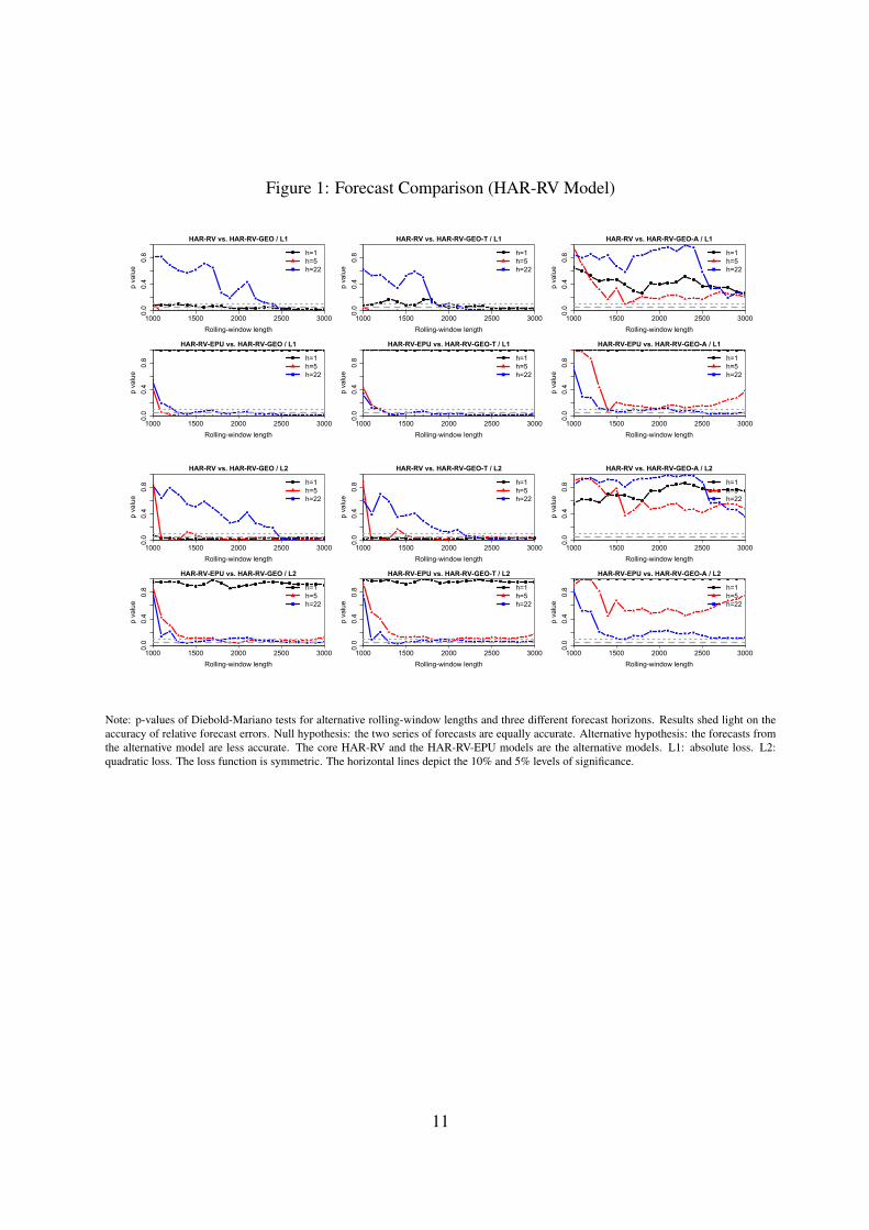
Figure 1: Forecast Comparison (HAR-RV Model)
1000 1500 2000 2500 3000
0.0
0.4
0.8
HAR-RV vs. HAR-RV-GEO / L1
Rolling-window length
p va
lue
h=1h=5h=22
1000 1500 2000 2500 3000
0.0
0.4
0.8
HAR-RV vs. HAR-RV-GEO-T / L1
Rolling-window length
p va
lue
h=1h=5h=22
1000 1500 2000 2500 3000
0.0
0.4
0.8
HAR-RV vs. HAR-RV-GEO-A / L1
Rolling-window length
p va
lue
h=1h=5h=22
1000 1500 2000 2500 3000
0.0
0.4
0.8
HAR-RV-EPU vs. HAR-RV-GEO / L1
Rolling-window length
p va
lue
h=1h=5h=22
1000 1500 2000 2500 3000
0.0
0.4
0.8
HAR-RV-EPU vs. HAR-RV-GEO-T / L1
Rolling-window length
p va
lue
h=1h=5h=22
1000 1500 2000 2500 3000
0.0
0.4
0.8
HAR-RV-EPU vs. HAR-RV-GEO-A / L1
Rolling-window length
p va
lue
h=1h=5h=22
1000 1500 2000 2500 3000
0.0
0.4
0.8
HAR-RV vs. HAR-RV-GEO / L2
Rolling-window length
p va
lue
h=1h=5h=22
1000 1500 2000 2500 3000
0.0
0.4
0.8
HAR-RV vs. HAR-RV-GEO-T / L2
Rolling-window length
p va
lue
h=1h=5h=22
1000 1500 2000 2500 3000
0.0
0.4
0.8
HAR-RV vs. HAR-RV-GEO-A / L2
Rolling-window lengthp
valu
e
h=1h=5h=22
1000 1500 2000 2500 3000
0.0
0.4
0.8
HAR-RV-EPU vs. HAR-RV-GEO / L2
Rolling-window length
p va
lue
h=1h=5h=22
1000 1500 2000 2500 3000
0.0
0.4
0.8
HAR-RV-EPU vs. HAR-RV-GEO-T / L2
Rolling-window length
p va
lue
h=1h=5h=22
1000 1500 2000 2500 3000
0.0
0.4
0.8
HAR-RV-EPU vs. HAR-RV-GEO-A / L2
Rolling-window length
p va
lue
h=1h=5h=22
Note: p-values of Diebold-Mariano tests for alternative rolling-window lengths and three different forecast horizons. Results shed light on theaccuracy of relative forecast errors. Null hypothesis: the two series of forecasts are equally accurate. Alternative hypothesis: the forecasts fromthe alternative model are less accurate. The core HAR-RV and the HAR-RV-EPU models are the alternative models. L1: absolute loss. L2:quadratic loss. The loss function is symmetric. The horizontal lines depict the 10% and 5% levels of significance.
11
Figu
re2:
Fore
cast
Com
pari
son
(QR
-HA
R-R
VM
odel
)
1000
1500
2000
2500
3000
0.2
0.4
0.6
0.8
HA
R-R
V vs
. GEO
/ L1
/ h=
1
Rol
ling-
win
dow
leng
th
α
1000
1500
2000
2500
3000
0.2
0.4
0.6
0.8
HA
R-R
V vs
. GEO
/ L1
/ h=
5
Rol
ling-
win
dow
leng
th
α
1000
1500
2000
2500
3000
0.2
0.4
0.6
0.8
HA
R-R
V vs
. GEO
/ L1
/ h=
22
Rol
ling-
win
dow
leng
th
α
1000
1500
2000
2500
3000
0.2
0.4
0.6
0.8
HA
R-R
V vs
. GEO
A /
L1 /
h=1
Rol
ling-
win
dow
leng
th
α
1000
1500
2000
2500
3000
0.2
0.4
0.6
0.8
HA
R-R
V vs
. GEO
A /
L1 /
h=5
Rol
ling-
win
dow
leng
th
α
1000
1500
2000
2500
3000
0.2
0.4
0.6
0.8
HA
R-R
V vs
. GEO
A /
L1 /
h=22
Rol
ling-
win
dow
leng
th
α
1000
1500
2000
2500
3000
0.2
0.4
0.6
0.8
HA
R-R
V vs
. GEO
T / L
1 / h
=1
Rol
ling-
win
dow
leng
th
α
1000
1500
2000
2500
3000
0.2
0.4
0.6
0.8
HA
R-R
V vs
. GEO
T / L
1 / h
=5
Rol
ling-
win
dow
leng
th
α
1000
1500
2000
2500
3000
0.2
0.4
0.6
0.8
HA
R-R
V vs
. GEO
T / L
1 / h
=22
Rol
ling-
win
dow
leng
th
α
Not
e:p-
valu
esof
Die
bold
-Mar
iano
test
sfo
ralte
rnat
ive
rolli
ng-w
indo
wle
ngth
san
dth
ree
diff
eren
tfor
ecas
thor
izon
s.R
esul
tssh
edlig
hton
the
accu
racy
ofre
lativ
efo
reca
ster
rors
.Nul
lhyp
othe
sis:
the
two
seri
esof
fore
cast
sar
eeq
ually
accu
rate
.Alte
rnat
ive
hypo
thes
is:
the
fore
cast
sfr
omth
eal
tern
ativ
em
odel
are
less
accu
rate
.The
core
HA
R-R
Vis
the
alte
rnat
ive
mod
el.T
hech
eck
func
tion
isth
elo
ssfu
nctio
n.T
hegr
ay(d
arkg
ray)
area
sde
note
resu
ltsth
atar
esi
gnifi
cant
atth
e10
%an
d5%
leve
lsof
sign
ifica
nce.
12
Figu
re3:
Fore
cast
Com
pari
son
(QR
-HA
R-R
VM
odel
With
EPU
)
1000
1500
2000
2500
3000
0.2
0.4
0.6
0.8
HA
R-R
V-EP
U v
s. G
EO /
L1 /
h=1
Rol
ling-
win
dow
leng
th
α
1000
1500
2000
2500
3000
0.2
0.4
0.6
0.8
HA
R-R
V-EP
U v
s. G
EO /
L1 /
h=5
Rol
ling-
win
dow
leng
th
α
1000
1500
2000
2500
3000
0.2
0.4
0.6
0.8
HA
R-R
V-EP
U v
s. G
EO /
L1 /
h=22
Rol
ling-
win
dow
leng
th
α
1000
1500
2000
2500
3000
0.2
0.4
0.6
0.8
HA
R-R
V-EP
U v
s. G
EOA
/ L1
/ h=
1
Rol
ling-
win
dow
leng
th
α
1000
1500
2000
2500
3000
0.2
0.4
0.6
0.8
HA
R-R
V-EP
U v
s. G
EOA
/ L1
/ h=
5
Rol
ling-
win
dow
leng
th
α
1000
1500
2000
2500
3000
0.2
0.4
0.6
0.8
HA
R-R
V-EP
U v
s. G
EOA
/ L1
/ h=
22
Rol
ling-
win
dow
leng
th
α
1000
1500
2000
2500
3000
0.2
0.4
0.6
0.8
HA
R-R
V-EP
U v
s. G
EOT
/ L1
/ h=1
Rol
ling-
win
dow
leng
th
α
1000
1500
2000
2500
3000
0.2
0.4
0.6
0.8
HA
R-R
V-EP
U v
s. G
EOT
/ L1
/ h=5
Rol
ling-
win
dow
leng
th
α
1000
1500
2000
2500
3000
0.2
0.4
0.6
0.8
HA
R-R
V-EP
U v
s. G
EOT
/ L1
/ h=2
2
Rol
ling-
win
dow
leng
th
α
Not
e:p-
valu
esof
Die
bold
-Mar
iano
test
sfo
ralte
rnat
ive
rolli
ng-w
indo
wle
ngth
san
dth
ree
diff
eren
tfor
ecas
thor
izon
s.R
esul
tssh
edlig
hton
the
accu
racy
ofre
lativ
efo
reca
ster
rors
.Nul
lhyp
othe
sis:
the
two
seri
esof
fore
cast
sar
eeq
ually
accu
rate
.A
ltern
ativ
ehy
poth
esis
:th
efo
reca
sts
from
the
alte
rnat
ive
mod
elar
ele
ssac
cura
te.
The
HA
R-R
V-E
PUm
odel
isth
eal
tern
ativ
em
odel
.T
hech
eck
func
tion
isth
elo
ssfu
nctio
n.T
hegr
ay(d
arkg
ray)
area
sde
note
resu
ltsth
atar
esi
gnifi
cant
atth
e10
%an
d5%
leve
lsof
sign
ifica
nce.
13