Realized Volatility, Heterogeneous Market Hypothesisand the Extended Wold Decomposition

Claudio Tebaldi

Bocconi University and IGIER

Conference in honor of J. Gatheral’s 60th birthdayCourant Institute NYU

October 14, 2017

1 / 55

Foreword on Impulse Response Functions

‘Dynamic economic models make predictions about impulse responses.....impulse responses quantify the exposure to long run macroeconomicshocks.... Financial markets provide compensations to investors who areexposed to these shocks.’J. Borovicka L. Hansen 2016

This exotic research program came to my mind...

World Bachelier Conference London 2008 Program

- 08.30-09.30 Plenary lecture: Lars Peter Hansen ”Modelling the longrun: valuation in dynamic stochastic economies”

- 09.30-10.30 Plenary lecture: Jim Gatheral ”Consistent modelling ofVIX and SPX options”

JIM .... YOU’RE RESPONSIBILE!2 / 55

Research Group on Impulse Response Functions

• OTT with F. Ortu and A. Tamoni “Long Run Risk and thePersistence of Consumption Shocks ”The Review of Financial Studies(2013), 26 (11) 2876-2915.

• BPTT with F.Bandi, B. Perron and A.Tamoni“The Scale ofPredictability”, forthcoming Journal of Econometrics.

• OSTT with F.Ortu, F. Severino and A.Tamoni “A persistence-basedWold-type decomposition for stationary time series”, WorkingPaper IGIER under review.

• CVOST Cerreia-Vioglio, S., Ortu, F., Severino, F., Tebaldi, C., 2017.Multivariate Wold Decompositions. Working Paper IGIER n.606,Bocconi University

• Rough Cascades and a potential resolution of Volatility and InterestRate Puzzles. Daniele D’Ascenzo (now JP Morgan) DanieleD’Arienzo Bocconi PhD Candidate

3 / 55

Motivation of the Talk

• Two well-established stylized facts that characterize economicfluctuations in dynamic economies and financial markets:

- The ‘multiscale’ nature of information based agent decisions: intrinsicfrequencies range from HFT trading decisions to secular trends.

- Widespread observation of self-similarity and scale invariance. The‘critical’ nature of economic fluctuations

• Research Program: explore the implications of these facts on impulseresponse functions with particular attention to their normative ratherthan descriptive implications.

• This talk: I will discuss the implications of these facts on log-volatilityIRf to conclude that there are important ”structural” motivationsthat suggest the introduction of a Rough Cascade Volatility Model.

4 / 55

Plan of the talk

• Impulse Response Functions in Dynamic Stochastic Economies.

• Fluctuations Theory and Critical Phenomena: Scaling, Universalityand Renormalization Group.

• The Extended Wold Decomposition.

• Heterogeneous Market Hypothesis, Resolution Filtration and Cascadesof Shocks.

• Volatility Forecasting with (Rough) Impulse Response Functions.

5 / 55

Literature on IRf

• Slutsky (1927), Yule (1927) and Frisch (1933) formulated theconcepts of “propagation” and “impulse” in economic time series.Wold (1938) formalizes the notion of IRF for a stationary time series.

• Identification challenges in rational expectation models Sims (1980).

• Hansen, Scheinkmann and Borovicka (2011-2016) introduce themodern non-linear continuous time extensions of IRf and its relationwith Malliavin Derivatives and Option sensitivities.

• Extension of the IRf as a relevant ’normative’ tool: see BoijnovShepard (2017) ‘Time series experiments and causal estimands’.

6 / 55

Classical Wold DecompositionGiven a zero-mean, regular, weakly stationary time series x = {xt}t∈Z, wehave

xt =+∞

∑h=0

αhεt−h + νt ∀t ∈ Z,

where the equality is in the L2-norm.

• The process ε = {εt}t∈Z is a unit variance white noise.

• αh is the projection coefficient of xt on the linear space generated bythe innovation εt−h:

αh = E [xtεt−h] , h ∈N0.

αh is the impulse response function of xt to the shock εt−h.

• The deterministic component ν is orthogonal to ε, id est

E [νtεt−h] = 0 ∀h ∈N0.

7 / 55

Fluctuations Theory and Critical Phenomena

• (Widom) scaling law for Magnetization

M (H,T ) = |t|β F(

H

|t|βδ

)t =

T − Tc

Tc

where function F is a universal scaling such that:

- M ∼ H1/δ for |t| = 0,

- M ∼ |t|β for H = 0 and |t| → 0

• Kadanoff’s idea was that in the critical regime a thermodynamicsystem, due to the strong correlations among the microscopicvariables, behaves as if constituted by rigid blocks of arbitrary size.

• Wilson Renormalization group: a semigroup of transformations thatproduces a progressive elimination of the microscopic degrees offreedom to obtain the asymptotic large scale properties of the system.

8 / 55

Renormalization Group in a Nutshell

• Renormalization Transformation and the Central Limit Theorem(Jona-Lasinio Phys. Reports 2001) Consider ξ1, ..., ξn, .... i.i.d. withzero mean and unit variance, and define block variables:

ζ1n = 2−n2

2n

∑i=1

ξi , ζ2n = 2−n2

2n+1

∑i=2n+1

ξi , then ζn+1 =ζ1n + ζ2n√

2

and correspondingly on the densities:

Rpζ

n :=∫

dypζ

n

(x√

2− y)p

ζ

n (y)

The fixed point of the transformation: Rpζ

∞ = pζ

∞ selects thestandard normal distribution.

9 / 55

Renormalization Group in a Nutshell II

• The action of R in the vicinity of the fixed point:

Rpζ

∞ (1 + ηh) = pζ

∞ (1 + ηLh) +O(η2)

defines a linear operator L:

Lh (x) :=2√π

∫dye−y

2h(x√

2− y)

• Eigenfunctions are given by Hermite functions hn

• Eigenvalues λn = 21−n2 , 0 ≤ n < 2 relevant directions, n = 2

marginal, n > 2 irrelevant.

10 / 55

Renormalization Group in a Nutshell III

• More generally the Renormalization Semigroup establishes a modifiedstochastic limiting procedure for stochastic correlated variables.E.g. Sinai defines an H− self similar process as a fixed point of a

rescaling transformation: ζn+1 =ζ1n+ζ2n2H

.

• Critical properties are determined by fixed points of proper RGprocedures that connect microscopic model critical correlations tomacroscopic observable behavior.

• Information on eigenvalues and eigenfunctions of the linearizedoperator provide information on critical indices and on finite sizescaling functions.

11 / 55

Rescaling Transformation on Time Series and DiscreteHaar filter

Multiresolution decomposition:

xt =J

∑j=1

g(j)t + π

(J)t ∀t ∈ Z.

• π(j)t is the average of size 2j of past values of xt :

π(j)t =

1

2j

2j−1∑p=0

xt−p.

• g(j)t is the difference between these averages:

g(j)t = π

(j−1)t − π

(j)t .

12 / 55

Rescaling Transformation and Persistence

• Variables g(j)t is associated with the level of persistence j : it captures

fluctuations of xt with half-life in [2j−1, 2j ). In this way, disentanglelow-frequency shocks from high-frequency fluctuations.

• Decimation procedure is necessary to get rid of the spuriouscorrelation due to the overlapping of observations in the construction

of g(j)t . Decimation selects the relevant degrees of freedom removing

redundant statistics.

• Decimated (detail) components g(j)t−2jk are proportional to Haar

Transform of the original time series and are in one-to-onerelationship with the original time series.

• However, even after decimation, variables g(j)t may be correlated, not

useful to define an IRf.

13 / 55

Redundant vs Decimated observationsThe Review of Financial Studies / v 0 n 0 2013

• • • • • • • • • •... g1 g2 g3 g4 g5 g6 g7 g8 ...

• • • • • • • • • •... g

(1)1 g

(1)2 g

(1)3 g

(1)4 g

(1)5 g

(1)6 g

(1)7 g

(1)8

...

• • • • • • • • • •... g

(2)1 g

(2)2 g

(2)3 g

(2)4 g

(2)5 g

(2)6 g

(2)7 g

(2)8

...

• • • • • • • • • •... π

(2)1 π

(2)2 π

(2)3 π

(2)4 π

(2)5 π

(2)6 π

(2)7 π

(2)8

...

t

j

Redundant decomposition

• • • • • • • • • •... g1 g2 g3 g4 g5 g6 g7 g8 ...

︸ ︷︷ ︸Block 1

︸ ︷︷ ︸Block 2

• • • • •... g

(1)2 g

(1)4 g

(1)6 g

(1)8

•••... g

(2)4 g

(2)8

•••... π

(2)4 π

(2)8

t

j

Decimated decomposition

(a)

(b)

Figure 1Redundant versus decimated decompositionThis figure displays the components of the time series gt before (Panel A) and after decimation (Panel B).

of the decimated components defined in (5) and (6) and then use the (inverseof the) operator T (J ) to reconstruct the process gt . We assume, in particular,that all decimated components are independent normal innovations, except forone which follows an autoregressive process on the time domain defined bydecimation. More formally, for t =k2j ,k∈Z, we let

g(j )t =ε(j )

t , ∀j <J ∗

g(J ∗)

t+2J∗ =ρJ ∗g(J ∗)t +ε(J ∗)

t+2J∗ , (11)

π(J ∗)t =η(J ∗)

t

with ε(j )t ∼N(0,2−j ), j <J ∗, ε

(J ∗)t ∼N(0,2−J ∗

(1−ρ2J ∗ )), and η

(J ∗)t ∼

N(0,2−J ∗). Finally, we assume that the serially independent innovations

ε(j )t , ε(j ′)

t are uncorrelated for j =j ′ and that ε(j )t is uncorrelated with η(J ∗)

t for

8

at Imperial College London Library on December 5, 2013http://rfs.oxfordjournals.org/

Downloaded from

14 / 55

The Abstract Wold Theorem

A general approach to derive orthogonal decompositions of time seriesfollows from the Abstract Wold Theorem, that involves an isometricoperator on a Hilbert space.

Theorem (Abstract Wold Theorem)

Consider a Hilbert space H and an isometry V : H −→ H, i.e.

〈Vx ,Vy〉 = 〈x , y〉 ∀x , y ∈ H.

Then H decomposes into an orthogonal sum H = H ⊕ H, where

H =+∞⋂

j=0

VjH, H =+∞⊕

j=0

VjLV

and the wandering subspace LV is defined as LV = HVH.

15 / 55

The Classical Wold Decompositionfrom the Abstract Wold Theorem

• The Classical Wold Decomposition follows from the Abstract WoldTheorem by considering the Hilbert space

Ht(x) = cl

{+∞

∑k=0

akxt−k :+∞

∑k=0

+∞

∑h=0

akahγ(k − h) < +∞

},

where γ : Z −→ R is the autocovariance function of x.

• The isometric operator that works on Ht(x) to obtain the ClassicalWold Decomposition is the lag operator:

L :+∞

∑k=0

akxt−k 7−→+∞

∑k=0

akxt−1−k .

16 / 55

The Extended Wold Decomposition: the set-up

The instrument is the Abstract Wold Theorem. Which isometric operator?

• We employ the Hilbert space

Ht(ε) =

{+∞

∑k=0

ak εt−k :+∞

∑k=0

a2k < +∞

},

i.e. the space spanned by the classical Wold innovations of x.

• Inspired by RG ideas, the isometry is the scaling operator

R :+∞

∑k=0

ak εt−k 7−→+∞

∑k=0

ak√2(εt−2k + εt−2k−1) .

17 / 55

The orthogonal decomposition of Ht(ε)

TheoremHt(ε) decomposes into the orthogonal sum

Ht(ε) =+∞⊕

j=1

Rj−1LRt ,

where

Rj−1LRt =

{+∞

∑k=0

b(j)k ε

(j)t−k2j ∈ Ht(ε) : b

(j)k ∈ R

},

with

ε(j)t =

1√2j

(2j−1−1∑i=0

εt−i −2j−1−1∑i=0

εt−2j−1−i

).

18 / 55

The decomposition of xt• Observe that (the purely non-deterministic part of) xt belongs toHt(ε).

• Denote, then, by g(j)t the projection of xt on Rj−1LR

t .

Proposition

Under the above conditions,

xt =+∞

∑j=1

g(j)t =

+∞

∑j=1

+∞

∑k=0

β(j)k ε

(j)t−k2j ,

where β(j)k = E

[xtε

(j)t−k2j

]is given by

β(j)k =

1√2j

(2j−1−1∑i=0

αk2j+i −2j−1−1∑i=0

αk2j+2j−1+i

).

19 / 55

The persistence-based Wold-type Decomposition Theorem

TheoremGiven a zero-mean, weakly stationary purely non-deterministic time seriesx = {xt}t∈Z, then

xt =+∞

∑j=1

g(j)t =

+∞

∑j=1

+∞

∑k=0

β(j)k ε

(j)t−k2j .

• For any scale j , the process{

ε(j)t−k2j

}k∈Z

is a unit variance white noise.

• The multiscale impulse responses β(j)k are unique, they do not depend on t

and ∑k

(β(j)k

)2< +∞.

• E[g(j)t−pg

(l)t−q]

depends at most on j , l , p − q and

E[g(j)t−m2j

g(l)

t−n2l]= 0 ∀j 6= l , ∀m, n ∈N0.

20 / 55

Resolution Filtration

SCA

LE

TIME t t-1 t-2 t-3 t-4

t-5

t-6 t-7 t-8

j=1

j=2

j=3

21 / 55

The decomposition of xt : remarks

• From now on, we call persistent component at scale j the quantity

g(j)t =

+∞

∑k=0

β(j)k ε

(j)t−k2j .

• When t is fixed, innovations of g(j)t have support

S(j)t = {t − k2j : k ∈ Z},

that becomes sparser and sparser as j increases.

• β(j)k is the multiscale impulse response associated with the innovation

at scale j and time shift k2j .

• Importantly, components at different scales are uncorrelated:

E[g(j)t g

(l)t

]= 0, j 6= l .

22 / 55

EWD forecasting and extensions

• Multivariate extension based on the theory of modules: β(j)k matrix of

impulse responses (OSTT and COST)

• Extension of the Beveridge Nelson permanent-transitorydecomposition (OST).

• Linear Forecasting theory for Wold decomposition induced byisometry R: is a discretized version of the linear forecasting theory forwide sense self-similar processes by Nuzman and Poor (2000, 2001).

• The dyadic non-linear extension of the IRf definition: GaussianStochastic Calculus of Variations (Malliavin Thalmeier 2006) see alsoStroock construction of Malliavin Calculus.

23 / 55

Estimation of multiscale IRFs

Given a weakly stationary time series x = {xt}t we estimate multiscaleIRFs in three steps:

1. estimate a suitable autoregressive form for x by exploiting AIC of BIC;

2. by operator inversion, turn the AR process into an MA and estimateclassical IRFs αh;

3. from coefficients αh, estimate multiscale IRFs β(j)k .

24 / 55

Simulations: multiscale IRF of an AR(2)

• Consider a weakly stationary purely non-deterministic AR(2)processes

xt = φ1xt−1 + φ2xt−2 + εt

• Compare two specifications φ1 = 1.16 and φ2 = −0.27 vs φ1 = 1.3and φ2 = −0.41.

• IRf at scale level j = 2, denote overreaction of the AR(2) process

• Scale levels j ≥ 3 have the same behaviour as the multiscale impulseresponse functions of an AR(1).

25 / 55

Simulations: multiscale IRFs of an AR(2)

0 2 4 6 8 10 12 14 16Lags k

0

0.2

0.4

0.6

0.8

1

1.2

1.4

Wol

d co

effic

ient

s,

k

(a) Impulse response function.

0 0.05 0.1 0.15 0.2 0.25 0.3 0.35 0.4 0.45 0.5Frequency

0

5

10

15

20

25

30

35

Pop

ulat

ion

dens

ity

(b) Spectrum.

-1

0

1Scale 1 --> [1, 2]

0 5 10 15 20 25 30

0

1

2

3Scale 2 --> [2, 4]

0 5 10 15 20 25 30

0

0.5

1Scale 3 --> [4, 8]

0 5 10 15 20 25 30

0

0.5

1Scale 4 --> [8, 16]

0 5 10 15 20 25 30

Lag

(c) Multiscale impulse responses.

-1

0

1Scale 1 --> [1, 2]

0 5 10 15 20 25 30

-10

-5

0

5Scale 2 --> [2, 4]

0 5 10 15 20 25 30

0

0.5

1Scale 3 --> [4, 8]

0 5 10 15 20 25 30

0

0.5

1Scale 4 --> [8, 16]

0 5 10 15 20 25 30

Lag

(d) Multiscale impulse responses.

Figure 1 Classical and multiscale impulse responses of two AR(2) processes: param-eters are set to φ1 = 1.16 and φ2 = −0.27 (blue dashed line in Panels A and B, andPanel C) and to φ1 = 1.3 and φ2 = −0.41 (red line with diamonds in Panels A andB, and Panel D). 20

26 / 55

Predictability of consumption growth components

• Run a regression component by component, namely:

∆cj ,t+1,t+2j = β0 + β1pdj ,t + εt+2j ,j

Scale j1 2 3 4 5 6 7 8

0.31 -0.49 -0.73 0.16 -0.17 -0.35 0.28 0.40pdt (0.74) (-1.75) (-2.88) (0.50) (-0.85) (-1.93) (2.56) (1.51)

[0.00] [0.01] [0.06] [0.01] [0.02] [0.24] [0.38] [0.01]

Table: The table reports OLS estimates of the regressors, correctedt-statistics in parentheses and adjusted R2 statistics in square brackets. Thesample spans the period 1947Q2-2009Q4.

• Long lasting cycles in consumption growth are forecasted by cycles ofcorresponding length in asset prices scaled by dividends

27 / 55

Identification of consumption drivers

• Which are the economic drivers of the predictable components ofconsumption growth?

• To determine these drivers we search for time series that are• characterized by an half-life close to the one of the component they are

to drive• correlated with such component

28 / 55

Identification - 3rd Component

• Our third component captures with a correlation of about 60% thealignment between consumption and investment decisions in thefourth quarter (fourth-quarter effect, e.g. Moller and Rangvid, 2010).

29 / 55

Identification - 6th Component

• Predictable components of consumption that occur at cycles between8 and 16 years reveal the position of the economy with respect to thetechnological cycle (e.g. Garleanu et al., 2009 and Kung and Schmid,2011), with a correlation of 64%.

30 / 55

Identification - 7th Component

• Our seventh component captures the alternating twenty-year periodsof booms and busts of US live births, with a correlation of about 44%.

Figure: The seventh component of consumption growth, g7,t along with ademographic variable, MYt , the middle-aged to young ratio proposed inGeanakoplos et al. (2004).

31 / 55

The Equity Premium

• Premium on the market return satisfies:

E [rm,t+1 − rf ,t ] +σ2m

2= λησ2

η + κ1,mλ′εQAm

Am =(

IJ − κ1,mdiag(

ρ))−1 (

φ− 1

ψ1

)Q = Et

[εt+1ε′t+1

]

where ρ = (ρ1, . . . , ρj , . . . , ρJ)′

• The vector λε determines the term structure of risk prices.

• The exposure to risks depends on QAm.

32 / 55

A calibration for equity premia

Use the estimate of ψ = 5 and calibrate γ = 5. Then the equity premia atdifferent scales are:

Scale j = Half-life (Years) Qj (1.0e − 005) Risk Exposure (1.0e-003) Risk Price Risk Premium (%)1 0.08 0.31 1.072 4.67 0.502 0.44 0.18 0.712 12.12 0.863 1.52 0.15 0.592 32.33 1.914 3.63 0.12 0.652 96.03 6.295 4.57 0.07 0.288 168.69 4.866 12.5 0.05 0.140 181.71 2.517 18.77 0.05 0.068 183.28 1.258 33.27 0.07 0.016 183.84 0.26

Table: This table reports equity premium (in %) Et [rm,t+1 − rf ,t ] decomposed bylevel of persistence.

33 / 55

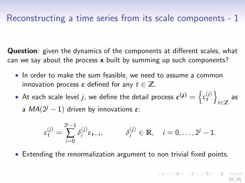
Reconstructing a time series from its scale components - 1

Question: given the dynamics of the components at different scales, whatcan we say about the process x built by summing up such components?

• In order to make the sum feasible, we need to assume a commoninnovation process ε defined for any t ∈ Z.

• At each scale level j , we define the detail process ε(j) ={

ε(j)t

}t∈Z

as

a MA(2j − 1) driven by innovations ε:

ε(j)t =

2j−1∑i=0

δ(j)i εt−i , δ

(j)i ∈ R, i = 0, . . . , 2j − 1.

• Extending the renormalization argument to non trivial fixed points.

34 / 55

Reconstructing a time series from its scale components - 2

We consider the processes g(j) ={g(j)t

}t∈Z

, with degree of persistence j ,

such that:

1)

g(j)t =

+∞

∑k=0

β(j)k ε

(j)t−k2j

2)+∞

∑j=1

+∞

∑h=0

(β(j)⌊

h2j

⌋δ(j)h−2j

⌊h2j

⌋

)2

< +∞

3) E[g(j)t−pg

(l)t−q]

depends at most on j , l , p − q and

E[g(j)t−m2j

g(l)t−n2l

]= 0 ∀j 6= l , ∀m, n ∈N0.

35 / 55

The Reconstruction Theorem

TheoremUnder the above assumptions, the process x = {xt}t∈Z defined by

xt =+∞

∑j=1

g(j)t

is zero-mean, weakly stationary purely non-deterministic and

xt =+∞

∑h=0

αhεt−h,

with

αh =+∞

∑j=1

β(j)⌊

h2j

⌋δ(j)h−2j

⌊h2j

⌋.

36 / 55

Reconstruction Theorem Remarks

• Different selection of δ(j)

h−2j⌊

h2j

⌋ select different renormalization

schemes that impact EWD and IRf.

• These coefficients are economically determined by the informationflows along the resolution filtration.

• Open Question: How competition shapes this flow in financialmarkets?

• Randomizes allocations of weights can be used to generateintermittency and clustering. Close to Kahane and Peyriere randomcascade models, Mandelbrot Calvet and Fisher’s multifractalvolatility.

37 / 55

Stochastic (log) volatility modelling

• Levy construction of the BM is that continuous time limit of theEWD generates the class of Brownian SemiStationary processes

xt = limJ→+∞

+∞

∑j=−J

x(j)t = lim

J→+∞

+∞

∑j=−J

+∞

∑k=0

β(j)k ε

(j)t−k2j =

∫ t

−∞g (t − s) dWs

• EWD Forecasting formulas:

Et [xt+∆] = Et

[+∞

∑j=−∞

x(j)t+∆

]=

+∞

∑j=−∞

+∞

∑k=0

β(j)k,∆ε

(j)t−k2j

38 / 55

Data and Realized Volatility

• Tick-by-tick series of USD/CHF exchange rate.

• Range: Dec1998 to Dec2003.

• Spot logarithmic middle prices computed (by Corsi) as averages of logbid and ask quotes.

• Returns are used to estimate daily realized volatility, as in Andersen,Bollerslev Diebold and Labys (2003):

dt =

√√√√M−1∑j=0

r2t−j/M , M = 12.

39 / 55

Persistence-based forecasting

• The Corsi forecasting equation exploits short-term lags of RealizedVolatility:

dt+1 = a0 + addt + awwt + ammt + νt . (1)

• Forecasting method based on the persistent components of dt thatexplain the most variance:

dt+1 = a(0) + a(7)Et

[d(7)t+1

]+ a(8)Et

[d(8)t+1

]+ a(9)Et

[d(9)t+1

]+ ξt .

• These three scales explain 44,6% of total variance. Same forecastingpower as Equation (1), but uncorrelated persistent components.

RMSE MAE R2

HAR-RV 2.607 1.757 0.565Extended Wold (3) 2.537 1.788 0.494

Extended Wold (10) 2.292 1.556 0.588

40 / 55

Variance decomposition of Realized Volatility

1 2 3 4 5 6 7 8 9 10Scale

0

0.05

0.1

0.15

0.2

0.25

0.3

Sca

le V

aria

nce

ove

r to

tal

Relative variance of daily RV

1 2 3 4 5 6 7 8 9 10Scale

0

0.05

0.1

0.15

0.2

0.25

0.3

Sca

le V

aria

nce

ove

r to

tal

Relative variance of weekly RV

1 2 3 4 5 6 7 8 9 10Scale

0

0.05

0.1

0.15

0.2

0.25

0.3

Sca

le V

aria

nce

ove

r to

tal

Relative variance of monthly RV

Figure 5 Variance ratio explained by each scale for daily, weekly and monthly RealizedVolatility.

0 5 10 15 20 25 30Lags

-0.6

-0.4

-0.2

0

0.2

0.4

0.6

0.8

1Sample ACFs

wmd(2)

d(4)

0 5 10 15 20 25 30Lags

-0.6

-0.4

-0.2

0

0.2

0.4

0.6

0.8

1Sample ACFs

d(7)

d(8)

d(9)

Figure 6 Left panel: comparison between sample ACFs of weekly and monthly RealizedVolatility (dashed and solid line respectively) with ACFs of persistent components of dailyRealized Volatility at scales 2 and 4 (lines marked with x and circles respectively). Rightpanel: sample ACFs of persistent components of daily Realized Volatility at scales 7 (dashedline), 8 (line marked with x) and 9 (line marked with circles).

33

1 2 3 4 5 6 7 8 9 10Scale

0

0.05

0.1

0.15

0.2

0.25

0.3

Scale

Varia

nce o

ver to

tal

Relative variance of daily RV

1 2 3 4 5 6 7 8 9 10Scale

0

0.05

0.1

0.15

0.2

0.25

0.3

Scale

Varia

nce o

ver to

tal

Relative variance of weekly RV

1 2 3 4 5 6 7 8 9 10Scale

0

0.05

0.1

0.15

0.2

0.25

0.3

Scale

Varia

nce o

ver to

tal

Relative variance of monthly RV

Figure 5 Variance ratio explained by each scale for daily, weekly and monthly RealizedVolatility.

0 5 10 15 20 25 30Lags

-0.6

-0.4

-0.2

0

0.2

0.4

0.6

0.8

1Sample ACFs

wmd(2)

d(4)

0 5 10 15 20 25 30Lags

-0.6

-0.4

-0.2

0

0.2

0.4

0.6

0.8

1Sample ACFs

d(7)

d(8)

d(9)

Figure 6 Left panel: comparison between sample ACFs of weekly and monthly RealizedVolatility (dashed and solid line respectively) with ACFs of persistent components of dailyRealized Volatility at scales 2 and 4 (lines marked with x and circles respectively). Rightpanel: sample ACFs of persistent components of daily Realized Volatility at scales 7 (dashedline), 8 (line marked with x) and 9 (line marked with circles).

33

41 / 55

Variance decomposition: remarks

• Volatility persistence is associated with the heterogeneous informationarrivals in the market (Andersen and Bollerslev 1997) and with thepresence of heterogeneous degree of persistence of information basedtrading (Muller et al. 1997)

• Evidence of the Heterogeneous Market Hypothesis. Data allows theestimation of 10 uncorrelated scales, which overall explain roughly95% of total sample variance.

• Persistence of the shocks: Shocks with degree of persistenceassociated to scales 7, 8 and 9 which involve that last 128, 256 and512 working days explain most of the variance variability.

42 / 55

Structural vs Descriptive interpretation of the EWD

An observation from a smart but inattent Referee:

‘In order to show the lack of structural interpretation, assume that thedata generating process is at a daily frequency. One could either observethe data at a daily frequency or at a weekly one. Each frequency will leadto a different DWT and I think that they are not strongly related, that isfor each scale (or horizon) the variables will be quite different.’

MAIN TAKEAWAY: A necessary condition for the decomposition to have astructural interpretation is a scale invariant aggregation scheme, i.e. theexistence of an RG fixed point.

43 / 55

Scale Invariance-1

0 0.5 1 1.5 2 2.5 3 3.5 4 4.5 5

log(∆)

-3.5

-3

-2.5

-2

-1.5

-1

-0.5

log(

m(q

,∆))

q=0.5q=1q=1.5q=2q=3

Figure 9: log(m(q,∆)) as a function of log(∆), FTSE 100.

Volatility extracted from empirical data since it exhibits some hallmarks of volatility such

as roughness and the alternation between periods of high and low volatility, the so-called

volatility clustering effect. This result is all the more significant considering the limited

number of parameters used.

Furthermore, to simulate the process, we exploited another property of volatility and

financial time series in general, that is their time multiscaling behavior. This means that

we can observe the same behavior and properties at different time scales and that, just by

time rescaling, we can retrieve kind of the same process. This is due to the fact that the

scaling TH is not growing rapidly since H is small. Hence, we first simulated the process

on a one day interval [0, 1] and then rescale it on a wider time period of 3500 days (almost

14 years), simply by multiplying v by 3500H .

24

44 / 55

Scale Invariance-2

0.5 1 1.5 2 2.5 3

q

0.05

0.1

0.15

0.2

0.25

0.3

0.35

0.4

ζ q

Figure 10: Scaling of ζq with q, FTSE 100.

4.1.3 The Correlation Structure of the RFSV

Another interesting property induced by this model is linked to the choice of an Hurst

parameter lower than 0.5 and concerns its correlation structure. Indeed, differently from

Comte and Renault that pick H > 0.5 to include long memory in their model, here log-

volatility is modeled as a short memory process. This is surprisingly since volatility has

been widely believed to be long memory, as evidenced in [2] and [24].

More specifically, Guegan [18] gives the following definition of long and short memory

processes:

Definition 4.1. A stationary process {Xt} is said to have long memory if its autocovari-

ances γ∆ are such that+∞∑

∆=−∞|γ∆| = +∞

25

45 / 55

Rough Volatility Cascade Model

• ”Volatility is rough” statement must be interpreted as the empiricalobservation that the macroscopic log-volatility dynamics is invariantw.r.t to a suitable RG scheme in the high frequency limit.

• This Prescription is sufficient to computation of the log-vol IRf.

RH :+∞

∑k=0

ak εt−k 7−→+∞

∑k=0

ak2H

(εt−2k + εt−2k−1)

will generate a properly defined EWD

log σt =+∞

∑j=1

g(j)t =

+∞

∑j=1

+∞

∑k=0

β(j)k ε

(j)t−k2j .

• The model in continuous time would look like the cascade model ofCalvet Fisher and Wu for interest rates with parametric restrictionsinduced by the ”Roughness Hypothesis” .

46 / 55

RCEWD-1

2013 2014 2015 2016 2017 2018-0.02

0

0.02Comp. 1

2013 2014 2015 2016 2017 2018-0.02

0

0.02Comp. 2

2013 2014 2015 2016 2017 2018-0.02

0

0.02Comp. 3

2013 2014 2015 2016 2017 2018-0.02

0

0.02Comp. 4

2013 2014 2015 2016 2017 2018-0.02

0

0.02Comp. 5

2013 2014 2015 2016 2017 2018-0.05

0

0.05Comp. 6

2013 2014 2015 2016 2017 2018-0.05

0

0.05Comp. 7

2013 2014 2015 2016 2017 2018-0.1

0

0.1Comp. 8

2013 2014 2015 2016 2017 2018-0.1

0

0.1Comp. 9

2013 2014 2015 2016 2017 2018-0.1

0

0.1Comp. 10

Figure 16: Estimated persistent components of daily Realized Volatility up to scale 10

from September 2013 to February 2017, FTSE 100.

36

47 / 55

RCEWD-2

with

Var(g

(j)t

)=

+∞∑

k=0

(β

(j)k

)2.

In this way, it is very easy to compute the percentage of variance explained by each

persistent component.

Figure 17 clearly shows that the persistent components with more explanatory power

are associated with scales 7, 8 and 9, which correspond to shocks lasting respectively 128,

256 and 512 days. This evidence supports the long-memory hypothesis.

1 2 3 4 5 6 7 8 9 10

Scale

0.02

0.04

0.06

0.08

0.1

0.12

0.14

0.16

0.18

0.2

0.22

Expl

aine

d Va

rianc

e

Figure 17: Percentage of total variance explained by each scale for daily Realized Volatil-

ity, FTSE 100.

Moreover, the same conclusion is reached with log-volatility data, for which the most

relevant components are those associated with scales 8, 9, 10, as can be seen from Figure

18.

37

48 / 55

RCEWD-3

0 100 200 300 400 500 600 700 800 900 10000

0.05

0.1

0.15

0.2

0.25

0.3

0.35

0.4

0.45

0.5Superimposed Actual and Predicted Volatilities (EWD)

Actual VolsPredicted Vols

Figure 19: Superimposed actual and predicted volatility (Extended Wold Decomposition),

FTSE 100.

6 Conclusion

The evidence of rough volatility has motivated different studies aimed at explaining and

reproducing this phenomenon. Among all, the RFSV model of Gatheral, Jaisson and

Rosenbaum [16] is of great interest since it links roughness to market microstructure

dynamics and models the irregular behavior of volatility in a simple way, using a frac-

tional Ornstein-Uhlenbeck process driven by a fBM with a Hurst parameter H < 12. This

provides interesting results in terms of representation of some stylized facts of volatility,

usually observed empirically, such as its low degree of smoothness and the volatility clus-

tering effect. Moreover it enables to reproduce in an easy manner the behavior of the

volatility surface extracted by option prices and, in particular, the explosion of the ATM

39

49 / 55

Conclusions and Future Developments

• Non-parametric discrimination among different Rough Vol Models

• A potential resolution of the long-term excess volatility puzzle andrough volatility cascade model.

• Ross recovery problem and Rough Volatility cascade model: betterunderstanding of the role of risk neutral vs historical measure

• Extension to the fractional case of the construction of the non-linearIRf extension Gaussian Stochastic Calculus of Variations andapplication to Option Hedging?

50 / 55

Barolo is good but Amarone is not bad ...

Happy Birthday Gino!

51 / 55

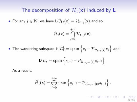
The decomposition of Ht(x) induced by L

• For any j ∈N, we have LjHt(x) = Ht−j (x) and so

Ht(x) =+∞⋂

j=0

Ht−j (x).

• The wandering subspace is LLt = span

{xt −PHt−1(x)xt

}and

LjLLt = span

{xt−j −PHt−j−1(x)xt−j

}.

As a result,

Ht(x) =+∞⊕

j=0

span{xt−j −PHt−j−1(x)xt−j

}.

52 / 55

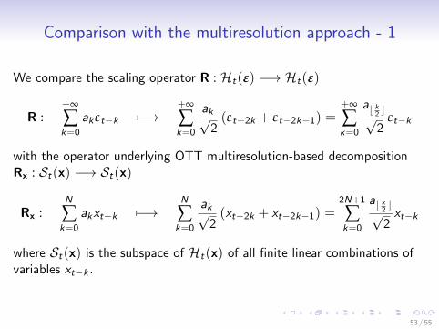
Comparison with the multiresolution approach - 1

We compare the scaling operator R : Ht(ε) −→ Ht(ε)

R :+∞

∑k=0

ak εt−k 7−→+∞

∑k=0

ak√2(εt−2k + εt−2k−1) =

+∞

∑k=0

ab k2 c√2

εt−k

with the operator underlying OTT multiresolution-based decompositionRx : St(x) −→ St(x)

Rx :N

∑k=0

akxt−k 7−→N

∑k=0

ak√2(xt−2k + xt−2k−1) =

2N+1

∑k=0

ab k2 c√2xt−k

where St(x) is the subspace of Ht(x) of all finite linear combinations ofvariables xt−k .

53 / 55

Comparison with the multiresolution approach - 2

• In case x is purely non-deterministic, St(x) ⊂ Ht(ε).

• Therefore, both R and Rx act on xt , providing two differentdecompositions.

• R is isometric and delivers the Extended Wold Decomposition;• Rx in general is not isometric and provides a multiresolution- based

decomposition that does not rule out correlation across scales.

• The main difference between the two decompositions is that the lagoperator and the scaling operator do not commute:

RL = L2R.

54 / 55

Comparison with the multiresolution approach - 3

Assume that limn γ(n) = 0.

• In the Extended Wold Decomposition,

xt =+∞

∑j=1

g(j)t with g

(j)t =

+∞

∑k=0

β(j)k ε

(j)t−k2j .

• In the multiresolution-based decomposition,

xt =+∞

∑j=1

g(j)t with g

(j)t =

+∞

∑h=0

αh√2j

ε(j)t−h.

55 / 55