The Role of Budget Stabilization Funds in Smoothing Government Expenditures Over the Business Cycle*

Gary A. Wagner**

A.J. Palumbo School of Business John F. Donahue Graduate School of Business

Duquesne University 600 Forbes Avenue

Pittsburgh, PA 15282 Phone: (412) 396-6241

Email: wagner@duq.edu

Erick M. Elder

Department of Economics & Finance University of Arkansas at Little Rock

2801 South University Avenue Little Rock, AR 72204 Phone: (501) 569-8879

Email: emelder@ualr.edu

December 2004

Abstract The economic downturn that began in 2001 resulted in massive budget shortfalls and arguably the worst fiscal conditions for state governments in nearly 50 years. States' use of savings to stabilize cyclical fluctuations in the budget has been institutionalized via budget stabilization funds. In this paper we explore how state expenditure volatility is affected by the existence, size, and structure of stabilization funds. The results indicate that while most states have not reduced the volatility of expenditures over the business cycle, states with rule-bound stabilization funds have witnessed significantly less expenditure volatility from utilizing a budget stabilization fund. JEL classification codes: H6, H7, G1 Keywords: fiscal policy, business cycles, budget stabilization funds, rainy day funds * The authors have benefited from discussions with David DeJong, Christopher Neely, George Hammond, Ronald Balvers, and seminar participants at the Federal Reserve Bank of St. Louis, West Virginia University, National Tax Association, and Southern Economic Association meetings. We also thank Edward Guidos for excellent research assistance. Wagner would also like to thank the A.J. Palumbo and John F. Donahue Schools of Business for financial support. Any remaining errors are the responsibility of the authors. ** Corresponding author

1

The Role of Budget Stabilization Funds in Smoothing Government Expenditures Over the Business Cycle

1. Introduction

During much of the 1990s, stock market gains and robust economic growth provided a windfall

of revenue that allowed state policymakers to enact sizable, permanent tax cuts. As economic

activity began to slow in 2001, the recently adopted tax cuts forced states into their worst fiscal

position in nearly 50 years. According to the National Governors Association (NGA), 40 states

were forced to reduce budgeted expenditures by nearly $12 billion in fiscal year 2003, which was

an increase from the 38 states that cut budgeted spending in 2002.1 In planning for fiscal year

2004, the NGA reports that 13 states enacted negative growth budgets and aggregate (nominal)

state spending is expected to grow at its slowest rate (0.2 percent) since 1979.

State policymakers rely heavily on expenditure reductions and tax increases to alleviate

budget shortfalls because, unlike the federal government, most states' options are constrained by

anti-deficit rules and borrowing restrictions (Poterba, 1994). And while states have an

established history of growing general fund surpluses during expansions to buffer future revenue

shocks, over the past 20 years nearly all states have institutionalized the use of savings via

budget stabilization funds (often referred to as "rainy day funds") to help smooth cyclical

fluctuations in the budget and lessen the sting of tax and expenditure adjustments. During fiscal

years 2002 and 2003 for instance, more than half of the 46 states with budget stabilization funds

relied on $8 billion from these instruments to help close budget gaps, which is considerably more

1 This information was obtained from the National Governor's Association Fiscal Survey of the States, December 2003. For a more thorough examination of the causes and consequences of the 2001 recession for state governments see Garrett and Wagner (2004).

2

than the $1 billion in stabilization fund balances tapped during the 1990-91 downturn (Holcombe

and Sobel, 1997).

The fact that properly structured BSFs can be a valuable tool to increase a state's savings

is well established in the literature. However, the extent to which BSFs permit state policymakers

to smooth expenditures or taxes over the business cycle, or simply retire debt, has yet to be

explored. Given states' experiences during the most recent downturn and the fact that expenditure

reductions and tax increases could contribute to the duration of a recession, understanding the

stabilizing role of BSFs is valuable. Using data that spans the entire history of budget

stabilization fund usage for nearly all states, this paper is the first to explore the role the

existence, size, and structure BSFs play in smoothing state-level expenditures over the business

cycle. We examine the role of BSFs in smoothing expenditures, as opposed to smoothing tax

rates or retiring debt, because Poterba (1994) finds that states are far more likely to increase

taxes in response to unexpected deficits than reduce expenditures, which suggests that

policymakers may be more interested in stabilizing expenditures than tax rates over the business

cycle.

The empirical results indicate that while the "average" state has not experienced a more

stable expenditure stream from utilizing a budget stabilization fund, we do find the degree of

expenditure smoothing to be directly related to the stringency of the deposit and withdrawal rules

governing the fund's operation. In other words, the empirical results show that states who adopt

and/or utilize more rule-bound stabilization funds experience significantly less expenditure

volatility than do states without (or with improperly structured) BSFs.

3

In the following sections of the paper we review previous research, present a theoretical

model of expenditure cyclicality, outline the empirical methodology and findings, and offer

concluding remarks.

2. Previous Research and Theoretical Framework

2.1 Background and previous research on budget stabilization funds

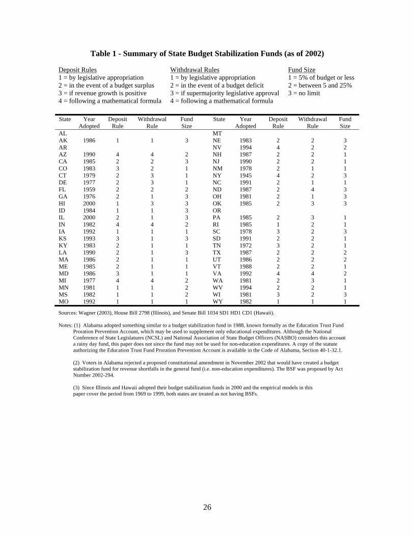
The expanded use of budget stabilization funds (hereafter "BSFs") over the past two decades

(noted below in Table 1) signals the growing importance policymakers place on savings to offset

revenue shortfalls. While more than 90 percent of states currently utilize a BSF, the most rapid

increase in usage occurred during the 1980s when 24 states adopted funds.

From the perspective of policymakers, budget stabilization funds may be a more

appealing tool for mitigating downturns than expenditure reductions and tax increase for several

reasons. First, expenditure reductions and tax increases, which may be necessary due to balanced

budget rules that prohibit deficits, are contractionary policies that may contribute to the duration

of a downturn. Second, the use of expenditure reductions and tax increases are politically costly.

For instance, Sobel (1998) finds that states with more discretionary increases in taxes and

reductions in expenditures during the 1990-91 recession have significantly higher turnover rates

in the legislature.

[Table 1 here]

The expanded use of BSFs is the primary reason why states relied on considerably more

BSF monies during the most recent downturn than during the 1990-91 recession. Rather than

maintaining a BSF balance equal to the allowable cap (see Table 1) or 5 percent of the budget as

4

bond ratings agencies suggest, most states have historically maintained a BSF balance between

1.5 and 3 percent of the budget.

Prior to the creation of budget stabilization funds, state governments regularly maintained

a general fund surplus during period of revenue growth for use during recessions. With the

addition of a BSF, states tend to maintain reserve balances in both the general fund and BSF

because the only practical difference between the two accounts is that while policymakers

deposit and withdraw surplus monies from the general fund at their discretion, deposits and

withdraws from BSFs tend to be governed by specific rules. As demonstrated in Table 1 for

example, 9 states deposit monies by legislative appropriation, 25 deposit funds only in the event

of a budget surplus, 6 states are required to deposit monies if revenue growth is positive, and 6

deposit funds in accordance with a pre-established formula.

While the difference between a BSF and general fund surplus may appear to be trivial,

previous research suggests that the fiscal benefits of utilizing a BSF depend highly on the

structure of the fund's deposit and withdrawal rules. Sobel and Holcombe (1996), Knight and

Levinson (1999), and Wagner (2003) find that states with more rule-bound (or "strict") BSFs,

meaning those funds that force deposits and limit withdraws, save significantly more than states

without BSFs or whose BSFs do not have such rules. Moreover, Wagner (2004) finds that states

with strict BSFs face significantly lower borrowing costs than states without BSFs. With regard

to the deposit and withdrawal rules in Table 1, category (3) and (4) rules are "strict" because they

require deposits and limit withdraws as long as the pre-established criteria are satisfied, while

category (1) and (2) rules are "weak" because they are based on legislative discretion.2

2 In the case of depositing in the event of a budget surplus, if a projected surplus exists for example, then policymakers may expand outlays, thereby lowering the required deposit to their BSF.

5

The fact that strict-rule BSFs have proven to be more effective than BSFs governed

largely by legislative discretion is not surprising because as Wagner (2003) notes, the extent to

which general fund surpluses and BSF balances are substitutable should depend on the

"closeness" of the BSF rules to legislative discretion: the more policymaker discretion over the

use of BSF monies, the more likely such monies will simply replace monies that were previously

maintained as a general fund surplus. In other words, the existence of strict-rule BSFs prevent

time inconsistency problems from arising while BSFs governed (effectively) by legislative

discretion do not. Thus, while policymakers may have a strong incentive to save during periods

of robust revenue growth (possibility to ensure their own long-term political survival), the

realization of a budget surplus also carries with it pressure from constituents and interest groups

to increase expenditures or reduce taxes. In the short-term, policymakers may find it in their best

interest to act on these pressures, thereby making previous plans to save time inconsistent. BSFs

governed by strict deposit and withdrawal rules provide policymakers with a mechanism that

may force their behavior to be time consistent and increases the likelihood that a state will be

better prepared for future downturns.

2.2 Theoretical model

In this section of the paper we develop a simple theoretical framework that may be used to

compare the volatility of government expenditures in a state without a BSF to the volatility in a

state with a "strict" BSF. A "strict" BSF is assumed to be a stabilization fund that is governed by

rules that force policymakers to deposit monies and limits when the monies may be accessed. We

develop a theoretical model for two reasons. First, the model allows us to better demonstrate why

a strict BSF smoothes spending. That is, is the decrease in spending volatility that we find

6

empirically associated with states with a BSF due to lower spending during high-revenue periods

or is the decreased spending volatility due to higher spending during low-revenue periods. An

alternative way of thinking about this issue is whether the strict deposit rules or strict withdrawal

rules that contribute more significantly to the decreased spending volatility. Strict deposit rules

limit a government’s ability to spend during high-revenue periods and force the government to

accumulate more savings which can be used to buffer spending cuts during future low-revenue

periods. Although it may seem obvious that strict deposit rules would result in smoother

spending patterns, it is not quite as obvious for the strict withdrawal rules. This ambiguity is

because on the one hand, strict withdrawal rules generally mean that, going forward, the

surpluses available to tap into in the case of a low-revenue period are larger which would tend to

contribute to smoother savings. On the other hand, strict withdrawal rules also limit a

government’s ability to smooth spending in the event of an actual low-revenue period. An

additional reason to develop a model is that a model allows us to develop testable implications

concerning the effects of prior budget surpluses and volatility of revenue on the volatility of

expenditures. In the context of the model, we first examine the optimal expenditure decisions of

an unconstrained government (one without a BSF), and then using a similar setup, impose

constraints concerning BSF deposits and withdraws.

The model assumes a forward-looking government who lives for two periods, t = 1, 2,

and faces uncertainty concerning current and future revenue. In each period revenue may be

either high or low, denoted as Rt ∈ Rt,H, Rt,L with Rt,H > Rt,L.3 The revenue process is assumed

to be described by a two-state Markov chain with conditional transition probabilities πij, denoting

P(R2 = R2j | R1 = R1i). We assume the government chooses a sequence for spending, Gt,

3 We assume R1L = R2L and R1H = R2H but retain the time subscripts for clarity.

7

(assuming tax rates are constant) to maximize expected utility given by a time separable utility

function:4

⎥⎦

⎤⎢⎣

⎡= ∑=

−2

1

100 )(

tt

t GuEUE β , (1)

where E0 is the expectation operator conditional on time 0 information. The government's

optimal spending in each period is contingent upon the realization of revenue in that period, and

second-period spending is conditional upon the realization of first-period revenue. To denote the

dependence on current period revenue, government spending is subscripted by the time period

and the realization of revenue, Gt,j, j = H, L.

We further assume the government maximizes expected utility subject to the constraint

that spending is non-negative. The government may enter period 1 with some accumulated

savings (debt), (1+r)S0, incurred from predecessors. If there is debt, the government does not

have to pay off the debt, but they must pay the interest on that debt. Because nearly all states

have a balanced-budget provision, we prohibit the government from spending that would require

issuing debt. Finally, the period-by-period budget constraint describes the evolution of

government savings is given by:

ttttt GSrRS −+=∆ −1 , (2)

where the change in savings, ∆St is the difference between revenue and interest received on

previous savings and total government spending (sum of government spending on goods and

services and transfer payments).

4 This is equivalent to assuming the government chooses spending to maximize the utility of a representative agent whose utility is a function of both private and public consumption and utility is separable in private and public consumption.

8

For each realization of first-period revenue, optimal first-period spending satisfies the

familiar Euler equation: )(')(' 21,1 GuERGu j β= for j=H,L. Assuming CRRA utility of the form

ρρ −−−= 11)1()( GGu , the first-order conditions for G1,j are:

[ ][ ] ⎪⎭

⎪⎬⎫

⎪⎩

⎪⎨⎧

−++++

+−+++++=

−

−

−ρ

ρρ

π

πβ

))1)((1(

))1)((1()1(

,1,10,2,

,1,10,2,,1

jjHHj

jjLLjj

GRSrrR

GRSrrRrG (3)

subject to the no debt restriction, G1,j ≤ (1+r)S0 + R1,j, j = H,L. The Euler equation equates the

marginal utility of spending an additional dollar in the first-period with the discounted expected

marginal utility of saving an additional dollar in the first-period. The uncertainty of second-

period revenue creates a potential precautionary motive to save, and in this sense, the model

above is a simplified model of the class of precautionary savings models developed by Zeldes

(1989), Deaton (1991), Kimball and Mankiw (1989), and Carroll (1992, 1997).

To incorporate BSFs into the model, the savings motive from a strict BSF can be

modeled by adding two additional constraints that describe deposits and withdraws from a

savings fund. In other words, if revenue is high, then a government with a BSF that has a strict

deposit rule must deposit an amount, δH, of the revenue into the BSF. Alternatively, if revenue is

low, then a government with a BSF that has a strict withdraw rule may withdraw an amount,

min(St-1,δL), from the BSF if the balance is positive. The simplest approach to formally modeling

these constraints is to express the constraints as limits on government expenditures. Hence, if

first-period revenue is high (and the government must deposit δH into their BSF), then G1,H ≤ R1H

- δH . And if first-period revenue is low, then G1,L ≤ R1L + min(S0,δL).

The optimal first-period spending, for each realization of revenue, for a government with

a strict BSF satisfies the Euler equation: )(')(' 21,1 GuERGu j β= for j=H,L,

9

[ ] ρ−ρ− −+++π+β= ))(1()1( ,1,10,2,,1 jjLLjj GRSrRrG (4)

subject to G1,H ≤ R1H - δH , G1,L ≤ R1L + min(S0,δL), and the no debt restriction. The difference

between equations (3) and (4) is that the last term in (3) no longer appears in (4). When second-

period revenue is high the government is required to save δH in the second period and spends the

remaining portion. Furthermore, if revenue is high in the second-period, then the government is

not able to access saved funds so the marginal utility of an additional saved dollar (in the first-

period) is zero and that term drops out of the first-order condition since G1,H ≤ R1H - δH .

The solution to equation (4) gives the optimal desired first-period spending levels for a

government with a strict BSF. If the desired spending level is greater then the constrained

spending level that may occur when the government is forced to deposit or withdraw funds from

the BSF, then the actual spending level will equal the constrained level. In terms of the model, if

G1,L > R1,L + δL then G1,L = R1,L + δL, and if G1,H > R1,H - δH then G1,H = R1,L - δH. If G1,L - R1,L <

δL, then the government does not withdraw as much as it could in the first-period (when R1=RL),

and likewise when R1,H - G1,H > δH , the government saves more than required in the first period

(when R1=RH).

Second-period spending is determined after solving equations (3) and (4) for G1,j, j =

H,L. The expected level of spending in each period, µt,G, is given by:

∑ ∑

∑

= =

=

==

=

LHkjkkj

LHjjG

LHiiiG

RRG

G

,1,2,

,,2

,,1,1

)|(ππµ

πµ (5)

where G2,k|R1 = Rj, j,k=H,L is second-period government spending when second-period revenue

is Rk given first-period revenue was Rj. To maintain consistency with the empirical work in

Section 3, we use the expected deviation from mean spending in the second period as the

10

measure of spending volatility. We concentrate on the second-period expected deviations to

focus attention on the “longer” term impact of BSF’s on spending volatility as opposed to the

immediate effects which are more closely proxied by the first-period expected deviations. The

second-period expected deviations from mean spending, E(D2), is:

( )∑ ∑= =

−==LHk

GjkkjLHj

j RRGDE,

,21,2,,

2 |)( µππ (6)

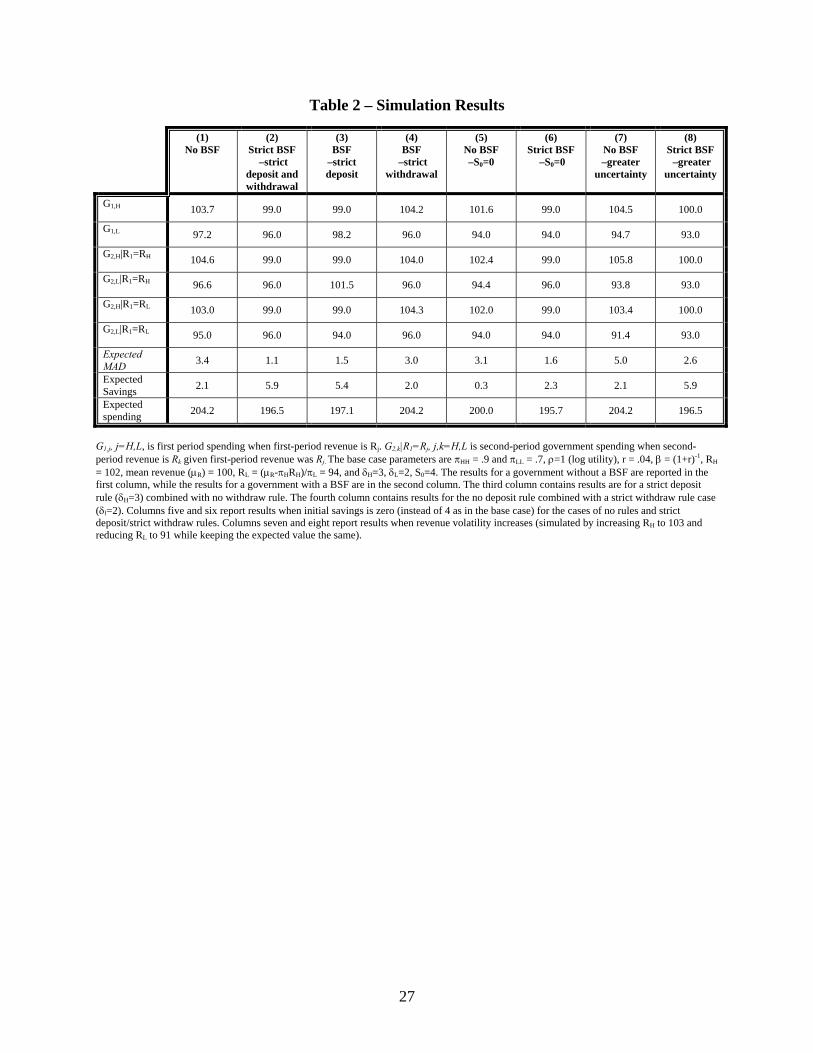
We simulate the model and assume the following parameter values for the base case: πHH

= .9 and πLL = .7, ρ=1 (log utility), r = .04, β = (1+r)-1, RH = 102, mean revenue (µR) = 100, RL =

(µR-πHRH)/πL = 94, and δH =3, δL = 2, S0 = 4.5 The simulated results are presented below in

Table 2.

[Table 2 here]

As columns 1 and 2 show, the expected volatility of expenditures, which is given in the

row labeled "Expected MAD" in Table 2, is lower for governments that require deposits and

limit withdraws (those with strict BSFs) than for governments that save at the discretion of

policymakers (those without BSFs). This is due to both the fact that governments with strict

BSFs have higher expected savings and are therefore better able to buffer expenditures against

future adverse revenue shocks as well as the fact that the strict rules limit spending in the second

period. It is also worth noting that governments with strict BSFs spend about 3.8 percent less

5 πH and πL are the unconditional probabilities of being in the high state and low state respectively. In addition, since we assume that the probability of a high realization of revenue is greater than a low realization of revenue, the size of a government's BSF balance will tend to infinity as the number of time periods tends to infinity. One simple solution to this problem is to set a threshold level of savings, S , above which deposits to a BSF are not required. In this case, governments would only be required to deposit a fraction of revenue in the BSF if revenue is high and savings is less than S . Alternatively, to prevent the BSF from tending to infinity, δL could be set (as a function of the δH and the transition probabilities) so that the unconditional expectation of the change in the BSF is zero. In practice, the first method of limiting the size of the BSF may be preferable since it does not require knowledge of the true transition probabilities.

11

than governments without BSFs (because of the forced deposits into the BSF), which may have

interesting dynamic effects on future tax rates, public sector growth, and income growth rates.

To explore the individual role of strict BSF deposit and withdrawal rules on expenditure

volatility, we separately examine the following cases: (1) a BSF is governed by a strict deposit

rule (δH=3) and no withdrawal rule, and (2) a BSF is governed by no deposit rule and a strict

withdrawal rule (δL=2). The results of these simulations are given in columns 3 and 4 of Table 2

respectively. As the results show, the volatility of expenditures diminishes slightly when only a

strict withdrawal rule is in place versus no BSF (neither strict withdrawal nor strict deposit

rules). This result is primarily due to the greater extent of depletion of savings for a “no BSF

state” (compared to a strict withdrawal BSF state) during a low-revenue first period which

ultimately results in lower spending in the second period regardless of the state of revenue. In

contrast however, a BSF governed by a strict deposit rule does result in significantly lower

expenditure volatility, but the reduction is not as large as when both strict deposit and strict

withdrawal rules are in place. The strict deposit rule significantly lowers spending volatility

(relative to a “no BSF state) because 1) the forced accumulation of savings during a high-

revenue first-period allows an increase in spending if the second period is a low-revenue period,

and 2) the strict deposit rule limits spending in a high-revenue second period. This finding

suggests that strict deposit rules have a much larger marginal effect on spending volatility than

strict withdraw rules.

Table 2 also compares the volatility of expenditures between regimes with and without

strict BSFs when initial savings (S0) is zero. These results are located in columns 5 and 6 and

illustrate that while both governments have higher volatility when initial savings is zero

12

(resulting from a reduced ability to buffer low realizations of revenue), governments with strict

BSFs continue to have higher expected savings and lower expected volatility.

The final two columns of Table 2, columns 7 and 8, illustrate how expenditure volatility

responds as revenue uncertainty rises (which is simulated by increasing RH to 103 and reducing

RL to 91 while keeping the expected value the same). In this scenario, expenditure volatility

increases for regimes without BSFs because there is a greater precautionary savings motive.

Expenditure volatility also rises for governments with BSFs (although it remains lower than

governments without such a fund) because the greater revenue volatility, which is manifested in

a larger gap between high and low revenue, increases the gap between what the government is

capable of spending when revenue is high and low, resulting in increased expenditure volatility.

3. Empirical Methodology

3.1 Measuring the cyclical variability in government expenditures

Recent studies of fiscal cyclicality, such as Lane (2003), measure cyclical variability using the

standard deviation in a cross-sectional framework. Specifically, Lane (2003) computes the

standard deviation of output growth for a given region over time and this measure is then

regressed on a set of fiscal policy and other control variables.

Since all but 4 states have adopted budget stabilization funds at various times over the

past 30 years, a cross-sectional framework along the lines of Lane (2003) is not feasible because

there is no suitable sample period from which we may compare states with BSFs to a sufficient

number of states without BSFs. As a result, we measure the cyclical variability of expenditures

using the absolute value of the cyclical component obtained by detrending real per capita

expenditures over the period from 1945 to 1999. To explore the robustness of the variability

13

measure and estimates, we decompose the trend and cyclical components of each state's real per

capita general fund expenditures using both the Hodrick-Prescott (1997) and band-pass filter

developed by Christiano and Fitzgerald (2003). Appendix B of the paper discusses both the

Hodrick-Prescott (HP) and band-pass (BP) filters in more detail.6

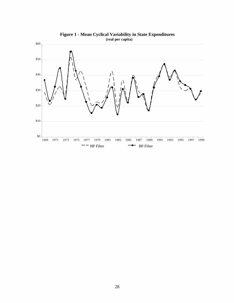
The mean cyclical variability in state expenditures (in absolute value), extracted

individually from each state using both the HP and BP filters, is illustrated below in Figure 1.

Overall, while the mean cyclical variability figures using the HP filter tend to be slightly larger

than the BP figures in most years, the turning points over the sample period are quite similar. In

addition, the HP and BP filters produce very comparable mean values, $31.15 and $30.44

respectively, when computed across all states and years.

[Figure 1 about here]

With regard to individual states, there are notable similarities and differences between the

HP and BP figures. For example, using the HP filter, Ohio has the smallest mean deviation from

trend ($17.72) and Virginia's cyclical variability has the smallest standard deviation ($11.43).

Interestingly, the positions of Ohio and Virginia switch when the cyclical variability is measured

by the BP filter – Virginia is found to have the smallest mean deviation from trend ($14.76),

while Ohio's cyclical variability has the smallest standard deviation ($11.50). In contrast, the HP

and BP filters generate remarkably similar figures on the high end. In both cases, Wyoming's

mean deviation from trend is the largest of all states ($68.87 with HP and $63.00 with BP) and

6 One potential problem with our methodology is that a state's trend level of real per capita expenditures may have changed following the adoption of a BSF. We explored this hypothesis for each state by regressing real per capita expenditures on a constant, linear trend, and an indicator variable that equals unity in each year that a state possesses a BSF. Using data over the period from 1945 to 1999 we were unable to reject the hypothesis that the BSF indicator equaled zero in each state except Connecticut and Wyoming. To ensure that the results in the paper were not being driven by Connecticut and Wyoming, we re-estimated each model excluding those states and found no qualitative differences in the results.

14

the cyclical variability in Mississippi's expenditures has the largest standard deviation of all

states ($105.36 with HP and $105.14 with BP).7

3.2 Empirical specification

The empirical model covers 46 states over the period from 1969 to 1999, resulting in 1426

observations.8 Given that only New York and Florida had BSFs in place prior to 1969, the

sample period covers the entire history of stabilization fund usage for most states. Denoting the

cyclical variability of real per capita expenditures in state i at time t as Gitσ , the empirical model

may be expressed as:

,,...,1 ;,...,1 : TtNiεγ ittiititGit ==+++++= θϕδασ BSFX (7)

where Xit is a vector of economic, political, and demographic factors in state i at time t assumed

to influence the cyclical variability of government expenditures, BSFit is a vector of budget

stabilization fund characteristics in state i at time t, iγ and tθ denote the fixed state- and time-

effects respectively, α is the constant term, itε is the error term, i is the index of the N states,

and t denotes the index of the T time periods. The inclusion of fixed time-effects will control for

aggregate shocks that may force state expenditures to deviate from trend, while the fixed state-

7 Although the cyclical component of state expenditures was extracted, for both the HP and BP filters, using data over the period from 1945 to 1999, the empirical models in the paper use the cyclical components over the period from 1969 to 1999 due to data limitations with other variables. The mean and standard deviation figures reported in Section 3.1 of the paper use the cyclical variability figures over the period from 1969 to 1999. 8 Hawaii and Alaska are excluded from the sample due to the fact that their economies differ greatly from other states. Nebraska and Minnesota were also excluded due to the fact they have, or have had, periods in which state legislators were elected without party designation, which made it impossible for us to determine the state's controlling political party. The starting period of our sample (1969) was based on the fact that the percentage of employees that are employed by state and local governments is not available prior to 1969, while the ending period of our sample (1999) comes from the fact that the Berry et al. ideology measures are not currently available past 1999.

15

effects will control for any time-invariant, state-specific factors that may affect expenditure

cyclicality.

Given Carlino and Sill's (2001) finding that there are regional trends and cycles in

income fluctuations at the state level, it is reasonable to assume that regional trends and cycles

may also be present in state-level expenditures, which suggests that the error term may be

correlated across states. As a result, we estimate equation (7) by Feasible Generalized Least

Squares (FGLS) and model the estimated covariance matrix as I ⊗Σ=Ω ˆˆ , where Σ is the cross-

sectional (NxN) matrix of estimated contemporaneous correlations and I is a TxT identity matrix.

Consistent with the theoretical model, we include the cyclical variability in a state's

revenue, cyclical variability of federal aid, cyclical variability of real per capita personal income,

and previous budget surplus/deficit as regressors. We expect increases in the cyclical volatility of

revenue, federal aid, and personal income to be positively correlated with expenditure

cyclicality, while increases in the previous budget surplus/deficit should be negatively correlated

with expenditure volatility. The revenue and federal aid variables will control for fluctuations in

revenue streams, the previous budget surplus/deficit will control for smoothing effects from a

state's other source (in addition to BSF monies) of savings, and the personal income variable will

control for state-specific economic shocks that may push expenditures away from trend.

To maintain consistency with the methodology for measuring expenditure cyclicality, we

measure revenue, personal income, and federal aid cyclicality as the absolute value of the

variable's real per capita cyclical component. The cyclical components are extracted to be

consistent with expenditures; if the cyclical component of expenditures is obtained via the HP

(BP) filter, then the cyclical components of all other variables measuring volatility are also

16

obtained using the HP (BP) filter. Complete descriptions, summary statistics, and sources for all

the variables may be found in Appendix A.

The model also includes several demographic variables that may affect a state's

expenditure volatility. First, we include the state's real per capita income to control for potential

income effects. Next, we include both the percentage of a state's residents age 65 and older and

the percentage of state employees employed by state and local governments as control variables.

Since the percentage of residents age 65 and older and government employees represent

powerful constituencies, we expect increases in these groups to result in greater volatility due to

the "voracity effect" described by Tornell and Lane (1999). Tornell and Lane argue that fiscal

competition may expand during upturns such that government spending may grow faster than

income grows, resulting in more volatile spending. Lane (2003) finds empirical support for this

"voracity effect" with government employees across OCED countries.

In addition to demographic factors, the empirical specification controls for fiscal

institutions that have been shown to have real economic effects.9 Specifically, the model includes

indicator variables for whether the state has a strict balanced budget rule that precludes fiscal-

year-end deficits and the existence of both expenditure and tax limitation laws. Since states with

strict balanced budget rules are forced to either reduce expenditures and/or increase taxes in the

event of a budget shortfall, we expect a stringent balanced budget rule to be positively correlated

with expenditure cyclicality, ceteris paribus. With regard to expenditure limitation laws, it is

plausible that such rules could either increase or decrease expenditure volatility, depending on

the volatility of real income growth. Given that expenditure limitation laws are generally based

on the growth in real personal income, a state with more volatile growth in real income may

9 For an overview of the effects of state fiscal institutions see Bohn and Inman (1996) and Poterba (1996).

17

experience more volatile expenditures since the "expenditure cap" will change with income

growth. On the other hand, we expect a binding tax limitation law to be associated with a

reduction in expenditure volatility, other factors constant, since it will limit the growth in

revenue during upturns and therefore should result in a more stable expenditure stream.

A number of recent studies, such as Gilligan and Matsusaka (1995), suggest that a state's

political climate influences fiscal behavior. To account for the state's political climate we

estimate equation (7) with an indicator variable that equals unity if the state's legislature and

Governorship are controlled by different parties.

The dynamic government and citizen ideology indices developed by Berry et al. (1998)

are also included as regressors. These ideology scores take on a value of 0 to 100, with 100 being

the most liberal value and 0 being the most conservative value. In combination with the state-

specific and time-specific fixed effects, the ideology measures should help control for

unobservable government and citizen tastes that could serve as a source of potential endogeneity

between expenditure cyclicality and the regressors.

Finally, the paper assesses the impact of BSFs on expenditure cyclicality by estimating

four separate regressions based on equation (7). First, Model (I) includes an indicator variable

that equals unity beginning with the year a state adopted a BSF and equals zero otherwise. This

specification will reveal, on average, how state expenditure cyclicality has changed as a result of

utilizing a BSF.

Next, Model (II) interacts the BSF adoption indicator with indicator variables reflecting

the various combinations of deposit and withdrawal rules. This will reveal how the volatility of

expenditures has changed following BSF adoption in states with different types of BSFs.

Specifically, Model (II) interacts the state's BSF adoption indicator with indicator variables for:

18

(1) strict deposit and strict withdrawal rules, (2) weak deposit and weak withdrawal rules, (3)

strict deposit and weak withdrawal rules, and (4) weak deposit and strict withdrawal rules. A

"strict" deposit/withdrawal rule is either a category (3) or (4) rule in Table 1, while a "weak"

deposit/withdrawal rule is either a category (1) or (2) rule. So, for instance, given that Kentucky

deposits monies to their BSF in the event of a budget surplus (a category (2) rule) and withdraws

monies via legislative discretion (a category (1) rule), Kentucky is considered to be a state that

has both a weak deposit and weak withdrawal rule. On the other hand, since South Carolina

deposits monies to their BSF each year that revenue growth is positive (a category (3) rule) and

withdraws monies in the event of a budget deficit (a category (2) rule), South Carolina is treated

as a state with a strict deposit and weak withdrawal rule. A complete list of the states that fall

into each category is provided in the notes to Appendix Table A1.

The final two models focus on how the size of a state's BSF influences expenditure

volatility. Model (III) includes the state's previous real per capita BSF balance as a regressor and

will reveal how the cyclical component of expenditures changes, on average across states, with a

$1 change in the state's per capita BSF balance. Model (IV), which interacts the state's previous

real per capita BSF balance with the four indicator variables reflecting the various deposit and

withdrawal rules, will provide an estimate of the marginal effect of a change in the BSF balance

on expenditure volatility in states with different types of BSFs.

4. Estimation Results

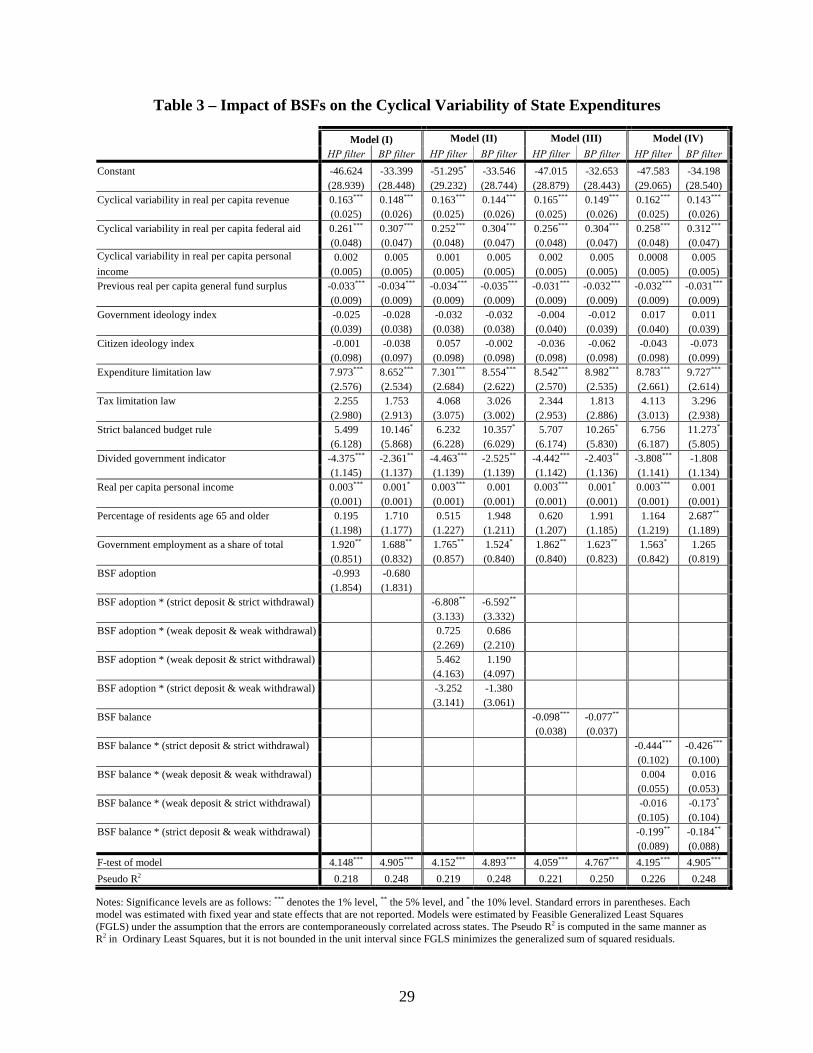
The results of the four adaptations of equation (7) are provided below in Table 3. Models (I), (II),

(III), and (IV) were each estimated by extracting the cyclical components using both the

Hodrick-Prescott (HP) and band-pass (BP) filters, resulting in a total of eight regressions.

19

[Table 3 here]

With the respect to the control variables, the estimates are generally robust across Models

(I) – (IV) and to the measurement of cyclicality. We find, for instance, that a $1 per capita

increase in the state's cyclical variability of revenue and federal aid results in a significant

increase in expenditure cyclicality of $0.14 - $0.16 and $0.25 - $0.31 respectively. Consistent

with the theory, more cyclical variability in a state's revenue sources results in greater

expenditure volatility, other factors constant.

In addition, the paper also finds that states that carry larger general fund surpluses have

significantly more stable expenditures, ceteris paribus. In fact, a $1 per capita increase in the

state's general fund surplus is found to reduce expenditure volatility by roughly $0.03, which is

significant at the 1 percent level and robust to the measurement of cyclicality. Although the

estimate is rather small, this result is consistent with Sorenson and Yosha's (2001) finding that

state surpluses are procyclical and promote stabilization. This result is consistent with the

theoretical results comparing Table 2 column 1 with 5 and column 2 with 6 which shows that a

larger initial surplus results in lower spending volatility.

The empirical estimates provide mixed results with respect to the political and ideology

variables. The dynamic citizen and government ideology measures, which are included in the

model to control for unobserved tastes that could serve as a source of potential endogeneity, are

not significantly different from zero in any of the specifications. In contrast, we do find that state

expenditures are significantly more stable during periods when the legislature and Governor are

members of different parties. This finding may reflect a political "tit-for-tat" in which the

legislature and Governor are forced to compromise.

20

Furthermore, the estimates of Models (I) – (IV) illustrate that demographic factors are in

important determinant of expenditure volatility. The paper finds that states with higher levels of

income and more government employees experience significantly more variability in

expenditures. With respect to government employees for instance, we find that a one percentage

point increase in the fraction of government employees (relative to total employment) results in a

$1.26 - $1.92 per capita increase in expenditure cyclicality. This result is consistent with Tornell

and Lane's (1999) "voracity effect" in which spending rises more proportionally than income

during expansions as a result of rent-seeking activities.

Expenditure limitation laws significantly increase the volatility of expenditures in the

range of $7.30 - $9.70 per capita, ceteris paribus. Since expenditure limit laws are typically

based on population growth and/or growth in real personal income, policymakers may both

"spend up to the cap" during expansionary periods and be forced to "cut spending to the cap"

during slowdowns, which could result in greater volatility. Given that the cyclical variability of

expenditures averages $31 per capita in our sample, our estimates for expenditure limitation laws

suggest that they increase the volatility of spending by 23 to 31 percent, other factors constant.

In contrast to expenditure limits, we find weak evidence that strict balanced budget rules

affect expenditure volatility and no evidence that tax limitation laws affect the volatility of

expenditures. A strict balanced budget rule significantly increases (at the 10 percent level)

expenditure volatility in the range of $10 - $11 per capita in the BP filter models, but we are

unable to reject the null hypothesis that balanced budget rules equal zero in the HP regressions.

Turning our attention to budget stabilization funds, the results from Models (I) – (IV)

yield tremendous insight into the role stabilization funds play in smoothing cyclical fluctuations

in government expenditures. Although Model (I) indicates that the average state has not

21

experienced a significant reduction in expenditure volatility following BSF adoption, Model (II)

reveals that states whose BSFs have both strict deposit and strict withdrawal rules have

experienced a $6.52 – $6.80 per capita reduction in expenditure volatility following adoption,

which is significant at the 5 percent level in both HP and BP specifications. This result is

consistent with the theoretical results comparing the expected MAD from Table 2 columns 1 and

2. Given the average expenditure volatility in our sample is $31 per capita, the results from

Models (I) and (II) indicate that states may reduce the cyclical variability of expenditures by 20

percent by adopting a BSF, but only if the BSF is governed by both strict deposit and strict

withdrawal rules.

The estimates from Models (III) and (IV) further confirm the importance of strict BSF

rules. While Model (III) demonstrates that the average state experiences a $0.07 – $0.09

reduction in expenditure volatility with a $1 increase in the size of the BSF, the results from

Model (IV) indicate that this finding is being driven by states with strict rules. For example, a

state with a strict deposit rule is able to reduce the cyclical component of expenditures by $0.18 –

$0.19 for every $1 increase in the BSF, while a state with both a strict deposit and strict

withdrawal rule reduces expenditure volatility by $0.42 – $0.44 with the same $1 increase in the

BSF balance. In contrast, states whose BSF is governed by either a weak deposit rule, or a weak

deposit and weak withdrawal rule, experience no change in the cyclical variability of

expenditures when additional funds are placed in the BSF. Consistent with the model results,

these empirical results indicate that while a strict deposit rule can result in lower expenditure

volatility (since it has greater marginal effect than a strict withdrawal rule), the presence of both

a strict deposit and strict withdrawal rule generates the greatest reduction in expenditure

volatility.

22

Overall, the estimates from Models (I) – (IV) generate some very clear conclusions and

implications. First, although a strict deposit rule reduces the cyclical variability of expenditures

compared to states without (or with ineffective) BSFs, a combination of rules that force deposits

and limit withdrawals generates the greatest expenditure smoothing and can provide

policymakers with a time-consistent stabilization vehicle. Thus, regardless of whether

policymakers view the objective of a BSF as a tool to mitigate revenue shocks during one fiscal

year or over a multi-year recession, our results suggest that the objectives may not be achieved

unless strict rules are in place.

Finally, while this paper addresses the limited question of expenditure smoothing, state

policymakers and/or voters may prefer to utilize stabilization fund balances to stabilize revenue

over the business cycle, which could be accomplished by reducing the number or size of tax

increases, or retire debt. Both of these options could, in theory, limit a state's ability to stabilize

expenditures over the business cycle and these issues remain unexplored in the literature. And

given that we find that a $1 increase in the BSF balance smoothes expenditures by less than $1,

our results suggest that exploring these options may be fruitful.

5. Conclusion

The fact that most U.S. states have institutionalized countercyclical fiscal policy through budget

stabilization funds (or "rainy day funds") provides a unique opportunity to explore the role of

fiscal policy as a means to promote stabilization. Using data that spans the entire history of

stabilization fund usage for nearly all states, this paper is the first to investigate how the

existence, size, and structure of budget stabilization funds impact the cyclical variability of state

government expenditures.

23

Controlling for the effects of demographic, political, and economic factors, we find that a

state's ability to smooth expenditures over the business cycle using a budget stabilization fund is

highly dependent on the structure of the deposit and withdrawal rules governing the fund.

Specifically, the results show that states whose policymakers have discretion over both deposits

and withdrawals experience no significant reduction in expenditure volatility compared to states

without stabilization funds, suggesting that such funds are tantamount to having no fund at all, at

least from the perspective of expenditure smoothing.

In contrast however, stabilization funds governed by one or more strict rules, meaning

those that actually require deposits or limit withdrawals, result in significant reductions in the

cyclical variability of expenditures. In fact, while we find that states with stabilization funds

governed by only one strict rule may experience more stable expenditure streams, states with

rule-bound budget stabilization funds witness reductions in the volatility of expenditures that are

nearly three times as large as states with only one stringent rule. This suggests that if government

policymakers are truly interested in smoothing expenditures over the business cycle, then

adopting a rule-bound budget stabilization can provide policymakers with a time-consistent tool

to achieve that goal.

Finally, the extent to which stabilization funds contribute to expenditure smoothing will

be dependent on policymakers' preferences for spending, taxes, debt, and the rate at which they

discount the future. These areas require additional research to determine what the objectives of

policymakers and/or voters are, and the role budget stabilization funds can play in achieving

those objectives.

24

References

Advisory Council on Intergovernmental Relations (ACIR) (1987), Fiscal Discipline in the Federal System: National Reform and the Experience of the States. Washington, D.C.: Advisory Council on Intergovernmental Relations.

Baxter, M., and R.G. King (1999), "Measuring Business Cycles: Approximate Band-Pass Filters

for Economic Time Series," Review of Economics and Statistics 81, 575-593. Berry, W.D., E.J. Rinquist, R.C. Fording, and R.L. Hanson (1998), "Measuring Citizen and

Government Ideology in the American States," American Journal of Political Science 42(1), 327-348.

Bohn, H., and Inman, R.P. (1996), "Balanced Budget Rules and Public Deficits: Evidence from

the U.S. States," NBER Working Paper No. 5533. Carlino, G., and K. Sill (2001), "Regional Income Fluctuations: Common Trends and Common

Cycles," Review of Economics and Statistics 83(3), 446-456. Carroll, C.D. (1992), "The Buffer-Stock Theory of Saving: Some Macroeconomic Evidence",

Brookings Papers on Economic Activity 1992:2, 61-156. Carroll, C.D. (1997), “Buffer-Stock Saving and the Life Cycle/Permanent Income Hypothesis”,

Quarterly Journal of Economics V. CXII, No. 1, 1-57. Christiano, L.J., and T.J. Fitzgerald (2003), "The Band Pass Filter," International Economic

Review 44(2). Deaton, A. (1991), "Savings and Liquidity Constraints", Econometrica LIX, 1221-48. Garrett, T.A., and G.A. Wagner (2004), "State Government Finances: World War II to the

Current Crisis, Federal Reserve Bank of St. Louis Review 86(2), 9-25. Gilligan, T.W., and J.G. Matsusaka (1995), "Deviations from Constituent Interests: The Role of

Legislative Structure and Political Parties in the States," Economic Inquiry 33, 383-401. Hodrick, R., and E. Prescott (1997), "Post-War Business Cycles: An Empirical Investigation,"

Journal of Money, Credit, and Banking 29(1), 1-16. Holcombe, R.G., and R.S. Sobel (1997), Growth and Variability in State Tax Revenue: An

Anatomy of State Fiscal Crises, Westport, CT: Greenwood Press. Knight, B., and A. Levinson (1999), "Rainy Day Funds and State Government Savings,"

National Tax Journal 52, 459-472.

25

Kimball, M.S., and N.G. Mankiw (1989), "Precautionary Savings and the Timing of Taxes", Journal of Political Economy 97(4), 863-879.

Lane, P. (2003), "The Cyclical Behaviour of Fiscal Policy: Evidence from the OECD," Journal

of Public Economics 87(12), 2661-2675. National Governors Association, Fiscal Survey of the States: December 2003, Washington, D.C.,

National Governors Association. Poterba, J. (1994), "State Responses to Fiscal Crises: The Effects of Budgetary Institutions and

Politics," Journal of Political Economy 102(4), 799-821. Poterba, J. (1996), "Budget Institutions and Fiscal Policy in the U.S. States," American

Economic Review 86, 395-400. Rueben, K. (1996), "Tax Limitations and Government Growth: The Effect of State Tax and

Expenditure Limits on State and Local Governments," unpublished manuscript, Massachusetts Institute of Technology.

Sobel, R.S. (1998), "The Political Costs of Tax Increases and Expenditure Reductions: Evidence

from State Legislative Turnover," Public Choice 96, 61-79. Sobel, R.S., and R.G. Holcombe (1996), "The Impact of State Rainy Day Funds in Easing State

Fiscal Crises During the 1990-1991 Recession," Public Budgeting and Finance, 28-48. Sorenson, B., and O. Yosha (2001), "Is State Fiscal Policy Asymmetric Over the Business

Cycle," Federal Reserve Bank of Kansas City Economic Review (Third Quarter), 43-64. Tornell, A., and P.R. Lane (1999), "The Voracity Effect," American Economic Review 89, 22-46. Wagner, G.A. (2003), "Are State Budget Stabilization Funds Only the Illusion of Savings?

Evidence from Stationary Panel Data," Quarterly Review of Economics & Finance 43(2), 213-238.

Wagner, G.A. (2004), "The Bond Market and Fiscal Institutions: Have Budget Stabilization

Funds Reduced State Borrowing Costs?" forthcoming in the National Tax Journal. Zeldes, S.P. (1989), "Optimal Consumption with Stochastic Income Deviations from Certainty

Equivalence", Quarterly Journal of Economics CIV, 275-98.

26

Table 1 - Summary of State Budget Stabilization Funds (as of 2002)

Deposit Rules Withdrawal Rules Fund Size 1 = by legislative appropriation 1 = by legislative appropriation 1 = 5% of budget or less 2 = in the event of a budget surplus 2 = in the event of a budget deficit 2 = between 5 and 25% 3 = if revenue growth is positive 3 = if supermajority legislative approval 3 = no limit 4 = following a mathematical formula 4 = following a mathematical formula

State Year

Adopted Deposit

Rule Withdrawal

Rule Fund Size

State Year Adopted

Deposit Rule

Withdrawal Rule

Fund Size

AL MT AK 1986 1 1 3 NE 1983 2 2 3 AR NV 1994 4 2 2 AZ 1990 4 4 2 NH 1987 2 2 1 CA 1985 2 2 3 NJ 1990 2 2 1 CO 1983 3 2 1 NM 1978 2 1 1 CT 1979 2 3 1 NY 1945 4 2 3 DE 1977 2 3 1 NC 1991 2 1 1 FL 1959 2 2 2 ND 1987 2 4 3 GA 1976 2 1 3 OH 1981 2 1 3 HI 2000 1 3 3 OK 1985 2 3 3 ID 1984 1 1 3 OR IL 2000 2 1 3 PA 1985 2 3 1 IN 1982 4 4 2 RI 1985 1 2 1 IA 1992 1 1 1 SC 1978 3 2 3 KS 1993 3 1 3 SD 1991 2 2 1 KY 1983 2 1 1 TN 1972 3 2 1 LA 1990 2 1 3 TX 1987 2 2 2 MA 1986 2 1 1 UT 1986 2 2 2 ME 1985 2 1 1 VT 1988 2 2 1 MD 1986 3 1 1 VA 1992 4 4 2 MI 1977 4 4 2 WA 1981 2 3 1 MN 1981 1 1 2 WV 1994 2 2 1 MS 1982 1 1 2 WI 1981 3 2 3 MO 1992 1 1 1 WY 1982 1 1 1

Sources: Wagner (2003), House Bill 2798 (Illinois), and Senate Bill 1034 SD1 HD1 CD1 (Hawaii).

Notes: (1) Alabama adopted something similar to a budget stabilization fund in 1988, known formally as the Education Trust Fund Proration Prevention Account, which may be used to supplement only educational expenditures. Although the National Conference of State Legislatures (NCSL) and National Association of State Budget Officers (NASBO) considers this account a rainy day fund, this paper does not since the fund may not be used for non-education expenditures. A copy of the statute authorizing the Education Trust Fund Proration Prevention Account is available in the Code of Alabama, Section 40-1-32.1.

(2) Voters in Alabama rejected a proposed constitutional amendment in November 2002 that would have created a budget stabilization fund for revenue shortfalls in the general fund (i.e. non-education expenditures). The BSF was proposed by Act Number 2002-294. (3) Since Illinois and Hawaii adopted their budget stabilization funds in 2000 and the empirical models in this paper cover the period from 1969 to 1999, both states are treated as not having BSFs.

27

Table 2 – Simulation Results

(1) No BSF

(2) Strict BSF

–strict deposit and withdrawal

(3) BSF

–strict deposit

(4) BSF

–strict withdrawal

(5) No BSF –S0=0

(6) Strict BSF

–S0=0

(7) No BSF –greater

uncertainty

(8) Strict BSF –greater

uncertainty

G1,H

103.7 99.0 99.0 104.2 101.6 99.0 104.5 100.0

G1,L

97.2 96.0 98.2 96.0 94.0 94.0 94.7 93.0

G2,H|R1=RH

104.6 99.0 99.0 104.0 102.4 99.0 105.8 100.0

G2,L|R1=RH

96.6 96.0 101.5 96.0 94.4 96.0 93.8 93.0

G2,H|R1=RL

103.0 99.0 99.0 104.3 102.0 99.0 103.4 100.0

G2,L|R1=RL

95.0 96.0 94.0 96.0 94.0 94.0 91.4 93.0

Expected MAD 3.4 1.1 1.5 3.0 3.1 1.6 5.0 2.6

Expected Savings 2.1 5.9 5.4 2.0 0.3 2.3 2.1 5.9

Expected spending 204.2 196.5 197.1 204.2 200.0 195.7 204.2 196.5

G1,j, j=H,L, is first period spending when first-period revenue is Rj. G2,k|R1=Rj, j,k=H,L is second-period government spending when second-period revenue is Rk given first-period revenue was Rj. The base case parameters are πHH = .9 and πLL = .7, ρ=1 (log utility), r = .04, β = (1+r)-1, RH = 102, mean revenue (µR) = 100, RL = (µR-πHRH)/πL = 94, and δH=3, δL=2, S0=4. The results for a government without a BSF are reported in the first column, while the results for a government with a BSF are in the second column. The third column contains results are for a strict deposit rule (δH=3) combined with no withdraw rule. The fourth column contains results for the no deposit rule combined with a strict withdraw rule case (δl=2). Columns five and six report results when initial savings is zero (instead of 4 as in the base case) for the cases of no rules and strict deposit/strict withdraw rules. Columns seven and eight report results when revenue volatility increases (simulated by increasing RH to 103 and reducing RL to 91 while keeping the expected value the same).

28

Figure 1 - Mean Cyclical Variability in State Expenditures

(real per capita)

$0

$10

$20

$30

$40

$50

$60

1969 1971 1973 1975 1977 1979 1981 1983 1985 1987 1989 1991 1993 1995 1997 1999

HP Filter BP Filter

29

Table 3 – Impact of BSFs on the Cyclical Variability of State Expenditures

Model (I) Model (II) Model (III) Model (IV) HP filter BP filter HP filter BP filter HP filter BP filter HP filter BP filter Constant -46.624 -33.399 -51.295* -33.546 -47.015 -32.653 -47.583 -34.198 (28.939) (28.448) (29.232) (28.744) (28.879) (28.443) (29.065) (28.540) Cyclical variability in real per capita revenue 0.163*** 0.148*** 0.163*** 0.144*** 0.165*** 0.149*** 0.162*** 0.143***

(0.025) (0.026) (0.025) (0.026) (0.025) (0.026) (0.025) (0.026) Cyclical variability in real per capita federal aid 0.261*** 0.307*** 0.252*** 0.304*** 0.256*** 0.304*** 0.258*** 0.312***

(0.048) (0.047) (0.048) (0.047) (0.048) (0.047) (0.048) (0.047) Cyclical variability in real per capita personal 0.002 0.005 0.001 0.005 0.002 0.005 0.0008 0.005 income (0.005) (0.005) (0.005) (0.005) (0.005) (0.005) (0.005) (0.005) Previous real per capita general fund surplus -0.033*** -0.034*** -0.034*** -0.035*** -0.031*** -0.032*** -0.032*** -0.031***

(0.009) (0.009) (0.009) (0.009) (0.009) (0.009) (0.009) (0.009) Government ideology index -0.025 -0.028 -0.032 -0.032 -0.004 -0.012 0.017 0.011 (0.039) (0.038) (0.038) (0.038) (0.040) (0.039) (0.040) (0.039) Citizen ideology index -0.001 -0.038 0.057 -0.002 -0.036 -0.062 -0.043 -0.073 (0.098) (0.097) (0.098) (0.098) (0.098) (0.098) (0.098) (0.099) Expenditure limitation law 7.973*** 8.652*** 7.301*** 8.554*** 8.542*** 8.982*** 8.783*** 9.727***

(2.576) (2.534) (2.684) (2.622) (2.570) (2.535) (2.661) (2.614) Tax limitation law 2.255 1.753 4.068 3.026 2.344 1.813 4.113 3.296 (2.980) (2.913) (3.075) (3.002) (2.953) (2.886) (3.013) (2.938) Strict balanced budget rule 5.499 10.146* 6.232 10.357* 5.707 10.265* 6.756 11.273*

(6.128) (5.868) (6.228) (6.029) (6.174) (5.830) (6.187) (5.805) Divided government indicator -4.375*** -2.361** -4.463*** -2.525** -4.442*** -2.403** -3.808*** -1.808

(1.145) (1.137) (1.139) (1.139) (1.142) (1.136) (1.141) (1.134) Real per capita personal income 0.003*** 0.001* 0.003*** 0.001 0.003*** 0.001* 0.003*** 0.001

(0.001) (0.001) (0.001) (0.001) (0.001) (0.001) (0.001) (0.001) Percentage of residents age 65 and older 0.195 1.710 0.515 1.948 0.620 1.991 1.164 2.687**

(1.198) (1.177) (1.227) (1.211) (1.207) (1.185) (1.219) (1.189) Government employment as a share of total 1.920** 1.688** 1.765** 1.524* 1.862** 1.623** 1.563* 1.265

(0.851) (0.832) (0.857) (0.840) (0.840) (0.823) (0.842) (0.819) BSF adoption -0.993 -0.680 (1.854) (1.831) BSF adoption * (strict deposit & strict withdrawal) -6.808** -6.592** (3.133) (3.332) BSF adoption * (weak deposit & weak withdrawal) 0.725 0.686 (2.269) (2.210) BSF adoption * (weak deposit & strict withdrawal) 5.462 1.190

(4.163) (4.097) BSF adoption * (strict deposit & weak withdrawal) -3.252 -1.380 (3.141) (3.061) BSF balance -0.098*** -0.077** (0.038) (0.037) BSF balance * (strict deposit & strict withdrawal) -0.444*** -0.426***

(0.102) (0.100) BSF balance * (weak deposit & weak withdrawal) 0.004 0.016 (0.055) (0.053) BSF balance * (weak deposit & strict withdrawal) -0.016 -0.173*

(0.105) (0.104) BSF balance * (strict deposit & weak withdrawal) -0.199** -0.184**

(0.089) (0.088) F-test of model 4.148*** 4.905*** 4.152*** 4.893*** 4.059*** 4.767*** 4.195*** 4.905***

Pseudo R2 0.218 0.248 0.219 0.248 0.221 0.250 0.226 0.248

Notes: Significance levels are as follows: *** denotes the 1% level, ** the 5% level, and * the 10% level. Standard errors in parentheses. Each model was estimated with fixed year and state effects that are not reported. Models were estimated by Feasible Generalized Least Squares (FGLS) under the assumption that the errors are contemporaneously correlated across states. The Pseudo R2 is computed in the same manner as R2 in Ordinary Least Squares, but it is not bounded in the unit interval since FGLS minimizes the generalized sum of squared residuals.

30

Appendix Table A1 – Variable Descriptions, Summary Statistics, & Sources (1969-1999)

Sample Mean (Std. Dev.)

Description Source

Cyclical variability in real per capita expenditures (Hodrick-Prescott filter)

31.1511 (33.1580)

Absolute value of deviation in real per capita expenditures from trend (trend estimated using HP filter)

Author's calculation using data from the Statistical Abstract of the United States

Cyclical variability in real per capita revenue (Hodrick-Prescott filter)

31.1652 (28.8957)

Absolute value of deviation in real per capita revenue from trend (trend estimated using HP filter)

Author's calculation using data from the Statistical Abstract of the United States

Cyclical variability in real per capita federal aid (Hodrick-Prescott filter)

16.7218 (15.7177)

Absolute value of deviation in real per capita federal aid from trend (trend estimated using HP filter)

Author's calculation using data from the Statistical Abstract of the United States

Cyclical variability in real per capita personal income (Hodrick-Prescott filter)

166.8117 (161.4042)

Absolute value of deviation in real per capita personal income from trend (trend estimated using HP filter)

Author's calculation using data from the Statistical Abstract of the United States

Previous real per capita general fund surplus/deficit

28.8909 (94.7400)

Real per capita general fund surplus/deficit lagged one year

Author's calculation using data from the Statistical Abstract of the United States

Government ideology index 48.1041 (22.6261)

Measure of government ideology [100=liberal; 0=conservative]

Berry et al (1998) and ICPSR #1208

Citizen ideology index 46.3288 (15.7375)

Measure of citizen ideology [100=liberal; 0=conservative]

Berry et al (1998) and ICPSR #1208

Divided government indicator 0.5302 (0.4993)

=1 if the legislature and governorship are controlled by different political parties, =0 otherwise

Book of States

Strict balanced budget rule 0.6990 (0.4626)

=1 state's BBR requires end-of-the-year fiscal adjustments to avoid a deficit, =0 otherwise

ACIR (1987)

Expenditure limitation law 0.1234 (0.3290)

=1 if state has a binding expenditure limit, =0 otherwise

Rueben (1996)

Tax limitation law 0.0554 (0.2288)

=1 if state has a binding tax limit, =0 otherwise

Rueben (1996)

Real per capita personal income

12705.5919 (2516.5253)

Real per capita personal income Bureau of Economic Analysis.

Percentage of residents age 65 and older 11.5547 (2.0409)

Percentage of the population age 65 and older

Bureau of the Census. Figure for 1969 was linearly interpolated.

Government employment as a share of total 13.6078 (2.5735)

State & local government employees as a share of total state employment

Bureau of Economic Analysis

BSF adoption indicator

0.4523 (0.4979)

=1 if the state has a BSF, =0 otherwise

Wagner (2003).

Previous real per capita BSF balance

9.4466 (21.5742)

Real per capita BSF balance lagged one year

Individual states & Statistical Abstract of the US

Strict deposit & strict withdrawal rule

0.0414 (0.1992)

=1 if state's BSF has a strict deposit & strict withdrawal rule, =0 otherwise

Wagner (2003)

Weak deposit & weak withdrawal rule

0.2356 (0.4245)

=1 if state's BSF has a weak deposit & weak withdrawal rule, =0 otherwise

Wagner (2003)

Weak deposit & strict withdrawal rule

0.0743 (0.2624)

=1 if state's BSF has a weak deposit & strict withdrawal rule, =0 otherwise

Wagner (2003)

Strict deposit & weak withdrawal rule

0.1010 (0.3014)

=1 if state's BSF has a strict deposit & weak withdrawal rule, =0 otherwise

Wagner (2003)

Notes: The following states are excluded from the sample: Alaska, Hawaii, Minnesota, and Nebraska. All real variables were deflated using the CPI-U (1982-1984=100). State population figures were obtained from the Bureau of Economic Analysis (BEA). Descriptive statistics for cyclical variability measures using the Band-Pass filter are not reported but are available from the authors. Expenditure and tax limitation laws are considered binding if they cannot be overridden by a simple majority vote of the legislature. Weak deposit and withdrawal rules are category (1) and (2) rules in Table 1, while strict rules are category (3) and (4) rules in Table 1. States with weak deposit and weak withdrawal rules are California, Florida, Georgia, Idaho, Illinois, Iowa, Kentucky, Louisiana, Maine, Massachusetts, Mississippi, Missouri, New Hampshire, New Jersey, New Mexico, North Carolina, Ohio, Rhode Island, South Dakota, Texas, Utah, Vermont, West Virginia, and Wyoming. Strict deposit and weak withdrawal rule states include Colorado, Kansas, Maryland, Nevada, New York, South Carolina, Tennessee, and Wisconsin. States with weak deposit and strict withdrawal rules are Connecticut, Delaware, North Dakota, Oklahoma, Pennsylvania, and Washington. Finally, strict deposit and strict withdrawal rule states include Arizona, Indiana, Michigan, and Virginia.

31

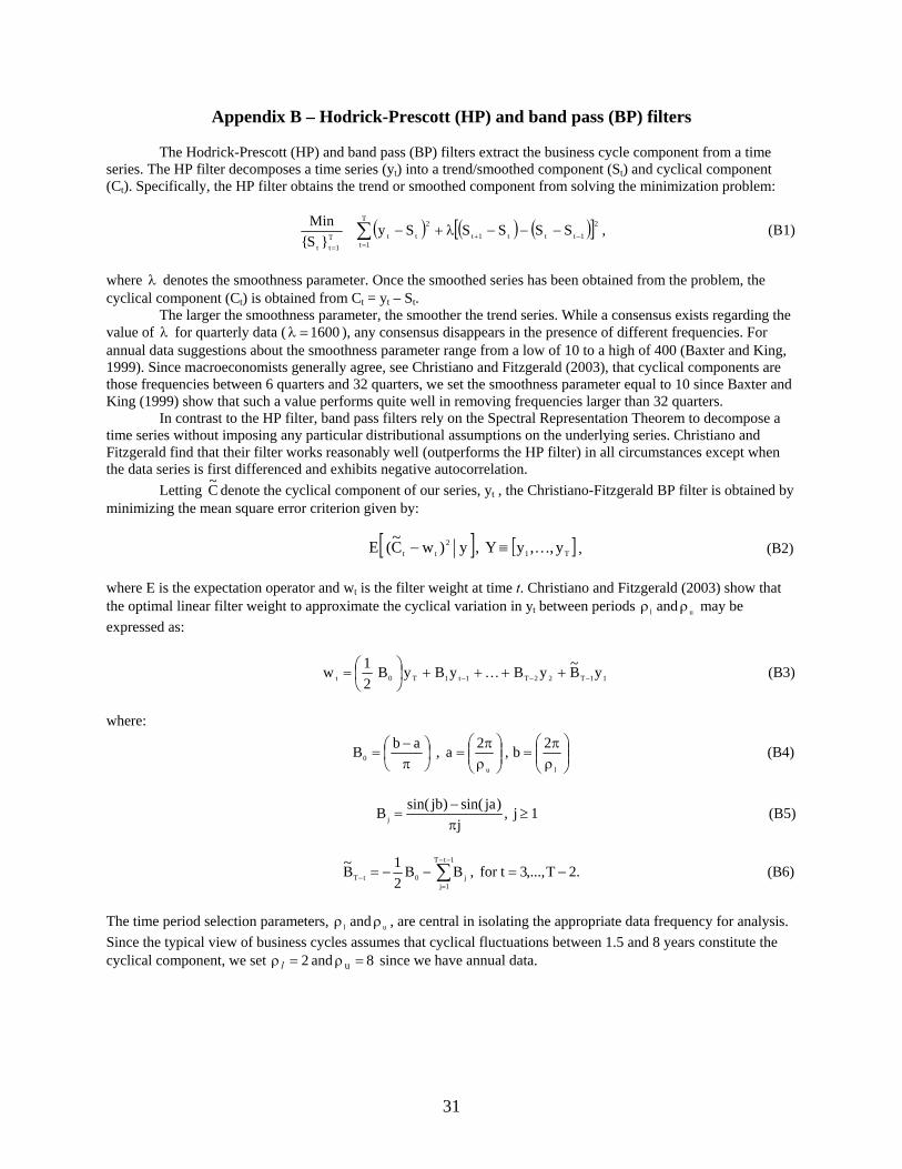
Appendix B – Hodrick-Prescott (HP) and band pass (BP) filters The Hodrick-Prescott (HP) and band pass (BP) filters extract the business cycle component from a time series. The HP filter decomposes a time series (yt) into a trend/smoothed component (St) and cyclical component (Ct). Specifically, the HP filter obtains the trend or smoothed component from solving the minimization problem:

( ) ( ) ( )[ ]21ttt1t

T

1t

2

ttT1tt

SSSSSyS

Min−+

==

−−−λ+−∑ , (B1)

where λ denotes the smoothness parameter. Once the smoothed series has been obtained from the problem, the cyclical component (Ct) is obtained from Ct = yt – St.

The larger the smoothness parameter, the smoother the trend series. While a consensus exists regarding the value of λ for quarterly data ( 1600=λ ), any consensus disappears in the presence of different frequencies. For annual data suggestions about the smoothness parameter range from a low of 10 to a high of 400 (Baxter and King, 1999). Since macroeconomists generally agree, see Christiano and Fitzgerald (2003), that cyclical components are those frequencies between 6 quarters and 32 quarters, we set the smoothness parameter equal to 10 since Baxter and King (1999) show that such a value performs quite well in removing frequencies larger than 32 quarters.

In contrast to the HP filter, band pass filters rely on the Spectral Representation Theorem to decompose a time series without imposing any particular distributional assumptions on the underlying series. Christiano and Fitzgerald find that their filter works reasonably well (outperforms the HP filter) in all circumstances except when the data series is first differenced and exhibits negative autocorrelation.

Letting C~ denote the cyclical component of our series, yt , the Christiano-Fitzgerald BP filter is obtained by minimizing the mean square error criterion given by:

[ ] [ ]T1

2tt y,,y Y, y)wC~(E K≡− , (B2)

where E is the expectation operator and wt is the filter weight at time t. Christiano and Fitzgerald (2003) show that the optimal linear filter weight to approximate the cyclical variation in yt between periods ul and ρρ may be expressed as:

11T22T1t1T0t yB~yByByB21w −−− ++++⎟

⎠⎞

⎜⎝⎛= K (B3)

where:

⎟⎠⎞

⎜⎝⎛

π−

=abB0 , ⎟⎟

⎠

⎞⎜⎜⎝

⎛ρπ

=⎟⎟⎠

⎞⎜⎜⎝

⎛ρπ

=lu

2b,2a (B4)

1j,j

)jasin()jbsin(Bj ≥π−

= (B5)

∑−−

=− −=−−=

1tT

1jj0tT .2T,...,3tfor , BB

21B~ (B6)

The time period selection parameters, ul and ρρ , are central in isolating the appropriate data frequency for analysis. Since the typical view of business cycles assumes that cyclical fluctuations between 1.5 and 8 years constitute the cyclical component, we set 8 and 2 u =ρ=ρ l since we have annual data.