the philippine review of economics - pep-net labor supply responses to adverse shocks under credit...
TRANSCRIPT

The Philippine Review of Economics

The Philippine Review of Economics
Volume XLV No. 2 December 2008 ISSN 1655-1516
1 Philippine economic nationalismGerardo P. Sicat
45 Labor supply responses to adverse shocks under credit constraints: evidence from Bukidnon, PhilippinesHazel Jean Malapit, Jade Eric Redoblado, Deanna Margarett Cabungcal-Dolor, and Jasmin Suministrado
87 Range-based models in estimating value-at-risk (VaR)Nikkin L. Beronilla and Dennis S. Mapa
101 Trading volume and serial correlation in stock returns in an emerging market: a case study of PakistanMohammed Nishat and Khalid Mustafa
119 Electoral cycles in Philippine fiscal and monetary policyDaryl Patrick Evangelista and Philip Amadeus Libre
161 Socio-economic determinants of childhood injuryClarissa V. Buenaventura and Ria F. Campos
185 Determinants of breastfeeding: the case of a Philippine urban barangayRachel M. Tanaka
205 The impact of family size on children’s school attendance in the PhilippinesKezia C. Bansagan and Hazel Joyce C. Panganiban
235 Democracy and poverty reductionVigile Marie B. Fabella and Czarina Eva I. Oyales
Articles
Book Review
271 Reasserting the rural development agenda: lessons learned and emerging challenges in AsiaLorelei C. Mendoza
PRE
Labor supply responses to adverse shocks under credit constraints:
evidence from Bukidnon, Philippines*
Hazel Jean Malapit, Jade Eric Redoblado, Deanna Margarett Cabungcal-Dolor, and Jasmin SuministradoAction for Economic Reforms; Graduate Program, UP School of Statistics; University of the Philippines College of Education; and Center for Conscious Living Foundation Inc., Philippines.
The ability of households to insure consumption from adverse shocks is an important aspect of vulnerability to poverty. How is consumption insurance achieved in a low-income setting where formal credit and insurance markets have been observed to be imperfect or missing? Using 2003 data from the Philippine province of Bukidnon, we investigate how labor supply is used to buffer transitory income shocks in light of credit constraints. We find that the most vulnerable households are those with little education and with few or no able-bodied male members. Appropriate policy responses include countercyclical workfare programs directed at households with high female-to-male ratios, households with high dependency ratios, and households with little or no education, as well as the provision of universal education and health care. These programs are likely to be effective in strengthening the labor endowments of households and improving their ability to cope with adverse shocks in the future.
JEL classification: J22, J43 Keywords: labor supply, credit constraints, consumption smoothing, coping strategies, idiosyncratic shocks, Philippines
* This work was carried out with financial and scientific support from the Poverty and Eco-nomic Policy (pep) Research Network, which is financed by the Australian Agency for Inter-national Development (AusaiD) and the Government of Canada through the International Development Research Centre (iDrc) and the Canadian International Development Agency (ciDa), and basis-crsp through the International Food Policy Research Network (ifpri).
The views represented in the paper are solely those of the authors and not necessarily of their respective institutions. The annexes are available upon request from the authors.
PRE THE PHILIPPINE REvIEW OF ECONOMICSVol. XlV no. 2 December 2008 p. 45-86

46 Malapit et al.: Labor supply adverse shocks and credit constraints
1. Introduction
The ability of families to cope with adverse shocks such as crop failure, unemployment, or illness is an important aspect of vulnerability to poverty. The increasing attention to risk and vulnerability arose from mounting evidence that shocks inflict permanent effects on human capital formation, nutrition, and incomes. The existence of poverty traps and other forms of persistence has shown that vulnerability to poverty is in itself a source of deprivation [Dercon 2001].
Well-being and poverty result from a complex decision process of households and individuals, given assets and incomes, and faced with risk. On the other hand, vulnerability is an ex ante concept, determined by the options available to the households and individuals to make a living, the risks they face, and their ability to handle these risks [Dercon 2001]. The ultimate effect of risk on the well-being of households and individuals depends largely on the coping strategies that may be employed by the household to protect consumption when adverse shocks occur.
How is consumption insurance achieved in a low-income setting where formal credit and insurance markets have been observed to be imperfect or missing? As noted by Kochar [1999], it is widely believed that consumption insurance is achieved through asset transactions, i.e., saving and dissaving. However, there is a variety of formal and informal mechanisms households may employ to insure consumption from fluctuations in income. These risk-management strategies include community risk-sharing (e.g., reciprocal arrangements, state-contingent remittances), income diversification, adoption of low-return low-risk crop and asset portfolios, savings depletion, sale of assets, borrowing, and ex post labor supply adjustments, among others.
Because labor is often the most abundant asset of the poor, this study attempts to measure the extent to which farm households use labor supplied to off-farm work in the face of adverse shocks and binding credit constraints. Moreover, this study investigates how this labor supply response differs between women and men, and the labor participation of school-age children. While previous research has concentrated on the “added worker effect” of wives to augment household income when their husbands become unemployed, this role need not be confined to married women. In fact, the Filipino norm of maintaining large households may be viewed as a risk-sharing arrangement, where secondary earners, adults and children, may be called upon to participate in the labor market to maintain household income when faced with a negative shock to household income.
This research differs from past studies in its explicit attention to both labor decisions and credit constraints.1 Intuitively, the smoothing role of the
1In the labor literature, the increase in household labor supply as a response to fluctuations in household income (e.g., unemployment of the breadwinner, crop failure) is referred to as
The Philippine Review of Economics, volume XLv No. 2 (December 2008) 47
secondary earners’ labor supply should be more important in the case of poorer households who cannot rely on asset depletion or borrowing to cope with the shock. The absence of a redistributive system of taxes or transfers, as well as the underdevelopment of insurance and credit markets, also contribute to the importance of secondary earners as the primary household coping mechanism. In the long run, the effects of adjustment costs to certain household members may erode the household’s ability to cope with future shocks, as is the case, for example, when children sacrifice schooling for work.
Household responses at the microlevel also translate to macrotrends in employment, education, and health outcomes, especially when shocks are aggregate in nature (e.g., economic crises and the like). The increasing volatility in world markets likewise increases the frequency and severity of aggregate shocks faced by ordinary households. A deeper understanding of how adjustment costs are borne within the household can inform social protection policy on where interventions are most necessary.
In his analysis of the effect of the East Asian crisis on the employment of women and men in the Philippines, Lim [2000] found that women have higher labor-force participation rates and longer working hours relative to men during the period. He also noted that high-school enrollment rates declined for both males and females, whereas elementary enrollment declined for females but not for males. Lim [2000] concluded that in times of crisis, and specifically in the East Asian crisis, there was a tendency toward “overworked” females and “underworked” males. He noted that maintaining and increasing labor-market participation of females not previously in the workforce appeared to be an important coping mechanism in the Philippines.
The objective of this paper is to analyze whether women and men increase their market labor supply in response to adverse shocks and in light of credit constraints. In particular, we attempt to answer the following question: Controlling for the effect of binding credit constraints, do women and men work more days off-farm when faced with adverse shocks?
Our analysis uses the 2003 data from Bukidnon, Philippines, collected by the International Food Policy Research Institute (ifpri) and the Research Institute for Mindanao Culture (rimcu), which allows us to investigate these issues using two sets of households: (a) “original” households, which are demographically older and correspond to the same households surveyed two decades ago in 1984-85, and (b) “split” households, which are new separate households formed by children of original households. Comparing our findings
the “added worker effect”. Because the presence of credit constraints limits the set of cop-ing strategies available to households, the “added worker effect” is expected to be stronger when households are unable to borrow to maintain consumption [Cullen and Gruber 1996; Lundberg 1985; Mincer 1962]. Labor supply was seldom studied explicitly within the context of credit constraints, with the exception of García-Escribano [2003].
48 Malapit et al.: Labor supply adverse shocks and credit constraints
for these two groups also allows us to investigate how labor supply responses to adverse shocks differ at earlier versus later stages of the life cycle.
2. Review of literature
This research builds on two separate strands of literature: (a) the consumption-smoothing literature, and (b) the literature on the smoothing role of secondary earners.
2.1. Consumption smoothing
The perfect risk-sharing hypothesis implies that, once aggregate shocks are accounted for, the growth rate of consumption would be independent of any idiosyncratic shock affecting the resources or income available to the household [Cochrane 1991; Deaton 1991; Townsend 1995; Skoufias and Quisumbing 2002]. Thus, the greater the correlation between household consumption and income, the less effective the risk-management strategy adopted by the household. This approach has also been used to assess the role of credit and savings as insurance substitutes, and make inferences on liquidity constraints2 [Skoufias and Quisumbing 2002].
Although empirical work on consumption smoothing has rejected the full risk-sharing hypothesis [Cochrane 1991; Townsend 1995], there is evidence that the overall effect of idiosyncratic income shocks on household consumption is not large. This implies that some mechanisms or channels, including those that in a first-best allocation would be considered sub-optimal, absorb most of the shocks [García-Escribano 2003].
Research on low-income economies (for example, see Morduch [1995]) show that households use a mix of formal and informal strategies to cope with adverse shocks, including community risk-sharing (e.g., reciprocal arrangements, state-contingent remittances), income diversification, adoption of low-return low-risk crop and asset portfolios, savings depletion, sale of assets, borrowing, and ex post labor supply adjustments. However, different households may have differential access to these strategies. Poorer households, in particular, may be less able to use strategies that rely on initial wealth as collateral [Skoufias and Quisumbing 2002]. On the other hand, it is often possible to adjust labor supply, regardless of initial wealth.
As noted by Kochar [1999], past research has demonstrated that farm households in developing countries are able to protect consumption from idiosyncratic shocks but offers little evidence on how this is achieved. To be able to understand the underlying economic environment, it is important to study how and to what extent specific mechanisms isolate consumption from the effect
2One key insight in the simulation results of Deaton [1991] is that a credit-constrained household may still be able to smooth consumption using precautionary savings, thus re-maining consistent with the permanent income hypothesis [Skoufias and Quisumbing 2002].

The Philippine Review of Economics, volume XLv No. 2 (December 2008) 49
of idiosyncratic income shocks. Much of the work on consumption smoothing has focused on the contribution of assets in buffering consumption variability [García-Escribano 2003; Kochar 1999]. However, these studies may not be relevant in explaining how consumption insurance is achieved in low-income communities, where asset levels may be low and access to credit limited.
2.2. Smoothing role of secondary earners
The literature exploring the role of secondary earners in smoothing transitory shocks to the household head’s earnings may be divided into two. The first set finds evidence of an insurance effect of secondary earners to the extent that it crowds out precautionary savings [Kochar 1995, 1999; Merrigan and Normandin 1996; Engen and Gruber 2001; Low 1999]. Kochar [1995, 1999] concludes that well-functioning labor markets in Indian villages allow households to increase labor income in response to crop shocks, reducing the need to resort to asset depletion or borrowing to smooth consumption. Using United Kingdom household data, Merrigan and Normandin [1996] found that precautionary motives are stronger for households with two earners compared to households with a single earner. Similarly, Engen and Gruber [2001] found that the effect of an increase in unemployment insurance on wealth holdings is smaller for married couples than for singles in the United States. Lastly, Low [1999] used numerical methods to show that precautionary savings in households with a secondary earner is smaller only if the correlation between shocks to the potential wages of the husband and wife is sufficiently negative.
The second set of literature explores the smoothing role of secondary earners through the “added worker effect”, which refers to the temporary increase in female labor supply (participation or hours worked) in response to transitory shocks to household income (excluding the wife’s income).3 Most studies estimate female employment or female hours worked as a function of the husband’s labor status together with standard covariates (e.g., labor market characteristics, household fixed effects). However, some studies have extended the definition of the husband’s (spouse’s) earnings loss to account for underemployment [Maloney 1991], idiosyncratic earnings shocks other than unemployment [García-Escribano 2002], and health shocks [Coile 2004].
The presence of liquidity constraints is one of the main arguments put forward in support of the existence of the “added worker effect” [Mincer 1962; Lundberg 1985; Cullen and Gruber 1996; Finegan and Margo 1994; García-Escribano 2003]. Cullen and Gruber [1996] reported evidence that families are liquidity-constrained during unemployment spells. This finding is consistent with Stephens [2001], where empirical results for layoffs are consistent with liquidity-constrained households. Similarly, García-Escribano [2003] found that households with limited credit access rely on the labor supply of wives to smooth the husband’s earnings shocks.
3See Malapit [2003] for a review of literature on the “added worker effect”.

50 Malapit et al.: Labor supply adverse shocks and credit constraints
The empirical results in the literature investigating the “added worker effect” remain mixed. Arguments put forward in support for the “added worker effect” include the substitutability of leisure of husbands and wives in home production [Ashenfelter 1980; Lundberg 1985; Maloney 1991], an income effect [Maloney 1991; Prieto and Rodriguez 2000], and the presence of liquidity constraints [Mincer 1962; Lundberg 1985; Cullen and Gruber 1996; Finegan and Margo 1994; García-Escribano 2003].
On the other hand, other factors that may obscure this effect include the following: assortative mating in tastes for work among spouses [Maloney 1991; Lundberg 1985; Cullen and Gruber 1996]; the wife’s employment factors are affected by the same factors causing the husband’s unemployment, or the “discouraged worker effect” [Serneels 2002; Prieto-Rodriguez and Rodriguez-Gutierrez 2000; Baslevent and Onaran 2001]; a crowding-out effect from social insurance programs [Cullen and Gruber 1996; Finegan and Margo 1994]; the value of the unemployment benefit is linked to the wage received by the wife [Cullen and Gruber 1996]; complementarity of leisure between spouses and care-giving needs [Coile 2004]; and different measurement approaches [Lundberg 1985].
Among the knowledge gaps that emerge from this brief review is the consideration of liquidity constraints. While it has been cited as the driving force for the “added worker effect” in the life-cycle context, few studies explicitly include liquidity constraints in their empirical models. This line of research is perhaps more relevant for rural areas in developing countries where credit markets are imperfect and there are little or no unemployment benefits.
In addition, only two studies extend the notion of the “added worker” to other family members [Serneels 2002; Kochar 1999], although in general, the “added worker effect” refers to all potential secondary earners in the family, including children. This point may have been irrelevant in the developed country context where households are often nuclear, but it is not so in the case of developing countries. A number of studies have linked child labor with income shortfalls and credit constraints [Jacoby and Skoufias 1997; Dehejia and Gatti 2002], emphasizing that parents may be forced to draw on their children’s labor when other strategies such as credit are not available.
Only a handful of studies on the “added worker effect” use data on developing countries, primarily as a consequence of the dearth of panel data. Such studies would also require analytical methods more suited to the specific labor market characteristics in the developing-country context. Also, sources of income shocks may be more diverse for agricultural households (not merely unemployment), and the “added worker effect” is relevant for all potential secondary workers, which include children. An exception is the work by Kochar [1999], which estimated hours of work responses to idiosyncratic crop shocks in rural India. Her model distinguishes labor supply by gender, and all household
The Philippine Review of Economics, volume XLv No. 2 (December 2008) 51
members aged fifteen to forty-five may contribute to labor income. However, her model does not accommodate credit constraints.
3. Conceptual framework
This section begins with a discussion of the agricultural household model to establish the theoretical relationships we wish to explore. Next, we discuss the theoretical treatment of permanent versus transitory shocks and their implications on market labor supply.
3.1. Agricultural household model
The model adopted here belongs to the subset of agricultural household models that investigate the impact of market imperfections on household decision making [Eswaran and Kotwal 1986; Carter and Zimmerman 2000]. This model assumes that the household acts as a single optimizing agent and, facing exogenous factor prices, maximizes per-period expected utility subject to a working-capital constraint and a time-endowment constraint [Eswaran and Kotwal 1986]. Farm output is a function of land and own-farm labor, and the linearly homogenous, increasing, strictly quasiconcave, and twice differentiable production function is given by
q f L h= ( ), ;ο θ
(1)
where hο is own-farm labor hours, L is land cultivated, and θ is the realization of weather and other crop income shocks. As in Eswaran and Kotwal [1986], we assume that production entails the incurrence of fixed setup costs (representing other inputs), K, and that each household has access to some amount β of working capital (including credit), typically determined by the amount of assets they possess. Finally, we assume the household’s utility function is defined over the present value of current period earnings, Y, and leisure: U Y l z Y u l z, ; ; ,( ) = + ( ) where z is a vector of observed and unobserved variables affecting preferences, and ′ > ′′ <u u0 0, .
The household’s optimization problem is thus given by
max , ;, , ,h h l L
mm p f L h wh v L L K u lο β θο
( ) + − −( ) − + ( )
(2)
s.t. B vL wh vL Km+ + ≥ + [working capital constraint] (2.1)
Ω − − − ≥h h lmο 0 [time-endowment constraint] (2.2)
L 0; 0; 0; 0≥ ≥ ≥ ≥h h lmο [time-endowment constraints] (2.3)

52 Malapit et al.: Labor supply adverse shocks and credit constraints
where β is the per period discount factor, L is land rented out, p is output price, w is the market wage, v is rent, and Ω is the time endowment. This model can easily be extended to distinguish the labor hours of members according to gender by disaggregating hours of work and wages for females and males.
This optimization yields market labor supply functions that depend on net access to working capital, output price, wage, rent, production shocks, and preference shifters.
h h B p w v zm m= ( ), , , ; ,θ (3)
where net access to working capital is given by the sum, B B K vL= − + . While the previous treatment assumes that the household will opt to
cultivate, Eswaran and Kotwal [1986] noted that a household would do so only if their maximized utility under cultivation exceeds that of being a pure agricultural worker. As pure agricultural workers, the household’s maximization problem is given by
U B L w v z B wh vL u h zhm m
m0* , , , ; max ;( ) = + + + −( )Ω
(4)
Therefore, the household will cultivate if and only if
U B p w v z U B L w v z* *, , , ; , , , , ;θ( ) > ( )0 (5)
While only production and preference shocks are introduced in this theoretical framework, a noncultivator household may experience shocks to their current income in the form of other adverse shocks, (Y – ε), in which case it is clear that the asset stock B will be used to buffer the impact of the shock. Households whose asset stocks are low are more likely to find that B < ε , and as such are expected to be credit-constrained.
3.2. Permanent versus transitory shocks
According to the permanent income hypothesis, consumption is constant over the life cycle and depends on permanent income. Temporary fluctuations in income are thus smoothed through credit and savings and should not affect consumption. Following this argument, only permanent shocks should affect labor decisions.
Contrary to the permanent income hypothesis, the “added worker” hypothesis predicts that negative transitory shocks to household income, through shocks on farm profits (e.g., crop failure) or earnings of other family members (e.g., unemployment), will result in a contemporaneous increase in market hours of work, all other things equal. The theory also implies that the increase in market hours of work will be temporary, and will no longer be necessary once the shock has subsided.
The Philippine Review of Economics, volume XLv No. 2 (December 2008) 53
In his classic article on female labor supply, Mincer [1962] showed that in a given period, the “temporary” reduction in family income due to the husband’s unemployment increases the probability that the wife will participate in the labor market in that period. He emphasized that this effect is expected when the family has few consumption-smoothing alternatives: “However, if assets are low or not liquid, and access to the capital market costly or nonexistent, it might be preferable to make the adjustment to a drop in family income on the money income side rather than on the money expenditure side … a transitory increase in labor force participation of the wife may well be an alternative to dissaving, asset decumulation, or increasing debt” [Mincer 1962].
On the other hand, Heckman and MaCurdy [1980] observed that “permanent” factors resulting in higher unemployment probability of the husband should increase the labor supply of wives over their lifetimes, and not only during the periods of unemployment. Thus, in a life-cycle setting, the “added worker effect” cannot be expected to be large unless in the presence of credit constraints [Lundberg 1985; Heckman and MaCurdy 1980]. Lundberg [1985] noted that without such a constraint, the wealth effect of a short unemployment spell is likely to be small, and contemporaneous movements in the labor supply of a married couple will reflect only cross-substitution effects, which are expected to be small.
Because the literature on the “added worker effect” refers to contemporaneous labor supply adjustments, we confine our study to the impact of negative shocks occurring in the current period on off-farm labor supply. If credit constraints are binding, both transitory and permanent shocks4 are expected to result in labor supply adjustments in the current period.
4. Data description
This study uses 2003 data from Bukidnon, Philippines, which is a resurvey of households from a four-round panel survey conducted in 1984-85. The household sampling procedure in 1984-85 was conducted using a quasi-experimental design to compare households that shifted to sugarcane production and households that did not, following the construction of a sugar mill in the province in 1977. The survey area extended beyond the neighborhood of the sugar mill, to include households that did not have the opportunity to adopt sugar (due to prohibitive transport costs) but shared a common farming environment and cultural heritage with sugar-adopting households [Bouis and Haddad 1990]. There were 448 households surveyed in all four rounds, and the last three rounds can be aggregated to comprise a full year.
4We are unable to classify shocks as “transitory” or “permanent” using econometric methods because this requires a panel data set. Instead, some shocks may be intuitively interpreted as transitory or permanent. For example, death of a household member is a permanent shock, while pest infestation is a transitory shock.
54 Malapit et al.: Labor supply adverse shocks and credit constraints
The 2003 data resurveys 305 of the core 448 households in 1984-85, as well as 257 new households formed by children from the original households who are now living in separate households.5 From these 562 households, we include 234 original and 229 split households who have both spouses present. Because the 1984-85 data provide very few variables on adverse shocks, we confine our labor supply analysis to the 2003 data.
4.1. Identifying credit-constrained households
As a general definition, we define a household to be credit-constrained if it would like to borrow, for whatever purpose, but cannot obtain credit from any source. We do not distinguish between formal and informal credit sources as they can function equally well in protecting consumption from income shocks.
One common method of testing for credit constraints is the consumption insurance hypothesis. If the growth rate of household consumption covaries with the growth rate of household income, then the household is said to be credit-constrained [Zeldes 1989]. However, one cannot simply look at the smoothness of consumption and know which mechanisms are at work. If labor income can be used to smooth consumption, consumption will appear to be insured even in the presence of binding credit constraints. Thus, to identify households that face binding credit constraints, a direct approach based on household responses to qualitative questions on credit will be necessary.
In the data, the question “If more credit were available for [purpose] in the past 12 months, would you have used it? Why not?” was included in the Assets, Backyard Production, Family Business, Farm Production, and Nonfood Expenditures blocks. Based on this question, households responding “Yes” to the qualitative question are classified as self-reported credit-constrained. We then constructed a summary indicator variable for credit constraints, where households are classified as credit-constrained if they answered “Yes” to the credit constraint question in at least one block.
4.2. Measuring household income shocks
From the theoretical model, labor-supply functions depend on a set of variables including farm profits, nonlabor income, and earnings of other household members. Shocks entering through any of these factors may result in adjustments in market labor supplied for credit-constrained households. Because our data deal with agricultural households, fluctuations in crop income are significant sources of household income shocks.
Several approaches may be used to measure crop income shocks. The first alternative is to use the residual from a profit regression [Kochar 1999]. Positive
5The 2003 survey initially surveyed 311 original households and 261 split households. Of these 572 households, ten households were dropped due to missing age and/or sex data for at least one of the household members.
The Philippine Review of Economics, volume XLv No. 2 (December 2008) 55
and negative residuals may be treated as separate shocks, since strategies used by households to respond to positive shocks are expected to be very different from strategies used to respond to negative shocks. One problem with this approach is that this residual contains unobserved variables that determine household expectations, as well as measurement error in profits. Because the profit regression excludes costs of family labor and other family-owned inputs, it also contains unobserved preference shocks that determine leisure choices.
The second alternative is to use standard instrumental variables techniques. This avoids the problems associated with the first approach if there is an instrument that is correlated with the “true” idiosyncratic crop shock, but not with preference shocks or measurement error in crop profits.
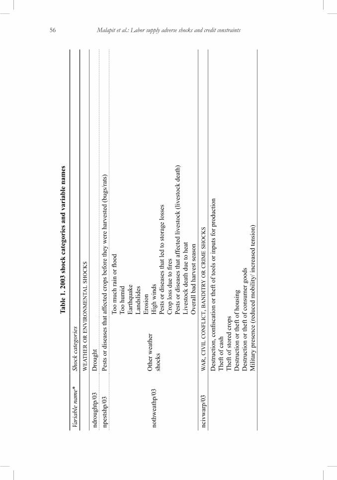
Although the Bukidnon data set provides a wide set of instruments,6 predicted crop income shocks obtained using instrumental variables techniques did not result in coefficient estimates significantly different from zero. Alternatively, we include self-reported incidents of adverse shocks occurring between 1984 and 2003. various sources of shocks are documented, including weather or environmental shocks affecting crops or livestock (e.g., drought, flooding, pests, diseases); war, civil conflict, banditry, and crime (e.g., theft, military presence); political, social, and legal events (e.g., confiscation of land, land reform); unexpected economic shocks (e.g., unemployment, severe lack of financing, severe inability to sell inputs); and unexpected events affecting health or welfare of members7 (e.g., death, illness, disablement, divorce, abandonment). Respondents are reminded that the shocks they report must have been difficult to foresee and must have significantly affected their households.
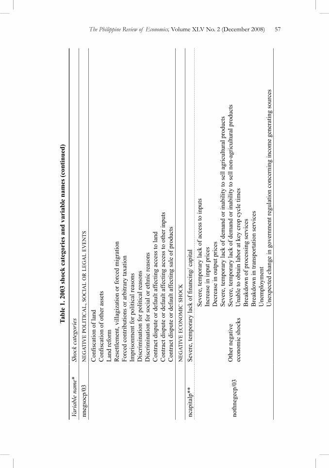
We construct count data for the number of incidents for each type of shock and distinguish between two time periods: past shocks are defined as occurring before 2003, while current shocks are defined as occurring in 2003. Table 1 presents a list of specific shock categories used in the analysis.
4.3. Descriptive statistics
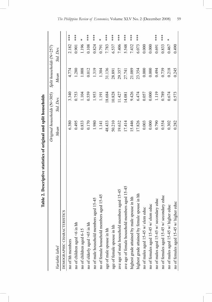
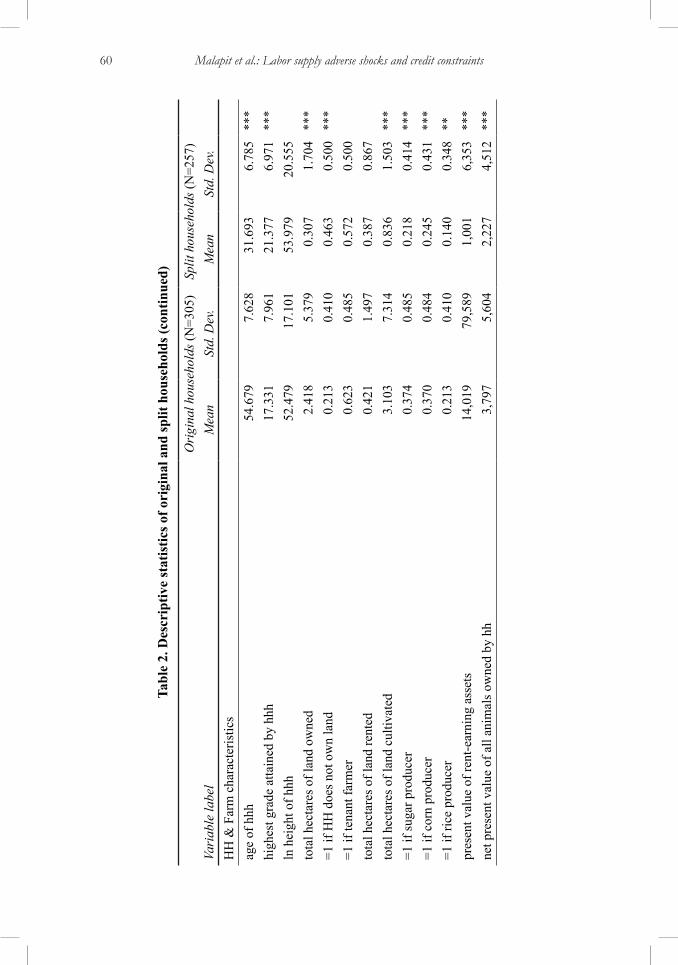
The means and standard deviations for selected variables are presented separately for original and split households in Table 2. As we expected, the two groups exhibited statistically significant differences in the means of a majority of the variables, reflecting the life-cycle differences between the two sets of households.
6Instruments used include rainfall deviations from the long-run average and incidents of crop failure due to drought and pests, as well as their interactions with farm characteristics (e.g., farm size, crop choice), and incidents and duration of illness by household members.7Shocks affecting the health and welfare of the household differ from the other shocks in that it can alter the labor endowment of the household. The effect of this type of shock on labor supply is ambiguous.
56 Malapit et al.: Labor supply adverse shocks and credit constraints
Tabl
e 1.
200
3 sh
ock
cate
gori
es a
nd v
aria
ble
nam
es
Vari
able
nam
e*Sh
ock
cate
gori
esw
eath
er o
r e
nv
iro
nm
enta
l sh
oc
ks
ndro
ught
p/03
Dro
ught
npes
tshp
/03
Pest
s or d
isea
ses t
hat a
ffect
ed c
rops
bef
ore
they
wer
e ha
rves
ted
(bug
s/ra
ts)
noth
wea
thp/
03O
ther
wea
ther
sh
ocks
Too
muc
h ra
in o
r floo
dTo
o hu
mid
Earth
quak
eLa
ndsl
ides
Eros
ion
Hig
h w
inds
Pest
s or d
isea
ses t
hat l
ed to
stor
age
loss
esC
rop
loss
due
to fi
res
Pest
s or d
isea
ses t
hat a
ffect
ed li
vest
ock
(live
stoc
k de
ath)
Live
stoc
k de
ath
due
to h
eat
Ove
rall
bad
harv
est s
easo
nnc
ivw
arp/
03w
ar
, civ
il c
on
flic
t, b
an
dit
ry o
r c
rim
e sh
oc
ks
Des
truct
ion,
con
fisca
tion
or th
eft o
f too
ls o
r inp
uts f
or p
rodu
ctio
nTh
eft o
f cas
hTh
eft o
f sto
red
crop
sD
estru
ctio
n or
thef
t of h
ousi
ngD
estru
ctio
n or
thef
t of c
onsu
mer
goo
dsM
ilita
ry p
rese
nce
(red
uced
mob
ility
/ inc
reas
ed te
nsio
n)
The Philippine Review of Economics, volume XLv No. 2 (December 2008) 57
Tabl
e 1.
200
3 sh
ock
cate
gori
es a
nd v
aria
ble
nam
es (c
ontin
ued)
Vari
able
nam
e*Sh
ock
cate
gori
esnn
egso
cp/0
3n
egat
ive
poli
tic
al,
so
cia
l o
r l
ega
l ev
ents
Con
fisca
tion
of la
ndC
onfis
catio
n of
oth
er a
sset
sLa
nd re
form
Res
ettle
men
t, vi
llagi
zatio
n or
forc
ed m
igra
tion
Forc
ed c
ontri
butio
ns o
r arb
itrar
y ta
xatio
nIm
pris
onm
ent f
or p
oliti
cal r
easo
nsD
iscr
imin
atio
n fo
r pol
itica
l rea
sons
Dis
crim
inat
ion
for s
ocia
l or e
thni
c re
ason
sC
ontra
ct d
ispu
te o
r def
ault
affe
ctin
g ac
cess
to la
ndC
ontra
ct d
ispu
te o
r def
ault
affe
ctin
g ac
cess
to o
ther
inpu
tsC
ontra
ct d
ispu
te o
r def
ault
affe
ctin
g sa
le o
f pro
duct
sn
egat
ive
eco
no
mic
sh
oc
k
ncap
italp
**Se
vere
, tem
pora
ry la
ck o
f fina
ncin
g/ c
apita
l
noth
nege
cp/0
3O
ther
neg
ativ
e ec
onom
ic sh
ocks
Seve
re, t
empo
rary
lack
of a
cces
s to
inpu
tsIn
crea
se in
inpu
t pric
esD
ecre
ase
in o
utpu
t pric
esSe
vere
, tem
pora
ry la
ck o
f dem
and
or in
abili
ty to
sell
agric
ultu
ral p
rodu
cts
Seve
re, t
empo
rary
lack
of d
eman
d or
inab
ility
to se
ll no
n-ag
ricul
tura
l pro
duct
sU
nabl
e to
obt
ain
labo
r at k
ey c
rop
cycl
e tim
esB
reak
dow
n of
pro
cess
ing
serv
ices
Bre
akdo
wn
in tr
ansp
orta
tion
serv
ices
Une
mpl
oym
ent
Une
xpec
ted
chan
ge in
gov
ernm
ent r
egul
atio
n co
ncer
ning
inco
me
gene
ratin
g so
urce
s

58 Malapit et al.: Labor supply adverse shocks and credit constraints
Tabl
e 1.
200
3 sh
ock
cate
gori
es a
nd v
aria
ble
nam
es (c
ontin
ued)
Vari
able
nam
e*Sh
ock
cate
gori
essh
oc
k r
ega
rd
ing
hea
lth
or
wel
far
e o
f h
ou
seh
old
ndea
thp/
03D
eath
Dea
th o
f hus
band
Dea
th o
f wife
Oth
er d
eath
nilln
essp
/03
Illne
ss
Illne
ss o
f hus
band
Illne
ss o
f wife
Oth
er il
lnes
sH
ospi
taliz
atio
n
noth
wel
fp/0
3O
ther
wel
fare
sh
ocks
Dis
able
men
t of w
orki
ng a
dult
hous
ehol
d m
embe
rsD
isab
lem
ent o
f oth
er h
ouse
hold
mem
bers
Div
orce
Aba
ndon
men
tD
ispu
tes w
ith e
xten
ded
fam
ily m
embe
rs re
gard
ing
land
Dis
pute
s with
ext
ende
d fa
mily
rega
rdin
g ot
her a
sset
sC
o-op
faile
d du
e to
mis
man
agem
ent
Une
xpec
ted
chan
ge in
gov
ernm
ent r
egul
atio
n co
ncer
ning
elig
ibili
ty fo
r pro
gram
atic
ass
ista
nce
*Sho
ck v
aria
bles
with
suffi
x “-
p” re
fer t
o pa
st sh
ocks
, occ
urrin
g be
twee
n 19
85 a
nd 2
002;
shoc
k va
riabl
es w
ith su
ffix
“-03
” re
fer t
o cu
rren
t sho
cks
occu
ring
in 2
003.
**nc
apita
l03
was
exc
lude
d be
caus
e m
ore
deta
iled
varia
bles
are
ava
ilabl
e fo
r cur
rent
per
iod
cred
it co
nstra
ints
.
The Philippine Review of Economics, volume XLv No. 2 (December 2008) 59
Tabl
e 2.
Des
crip
tive
stat
istic
s of o
rigi
nal a
nd sp
lit h
ouse
hold
s
Ori
gina
l hou
seho
lds (
N=3
05)
Split
hou
seho
lds (
N=2
57)
Vari
able
labe
lM
ean
Std.
Dev
.M
ean
Std.
Dev
.d
emo
gr
aph
ic c
ha
ra
cte
ris
tic
s
no o
f hh
mem
bers
6.38
03.
340
4.77
42.
182
***
no o
f chi
ldre
n ag
ed <
6 in
hh
0.49
50.
753
1.28
00.
901
***
no o
f chi
ldre
n ag
ed 6
-15
0.83
31.
104
1.00
81.
196
*no
of e
lder
ly a
ged
>65
in h
h0.
170
0.55
90.
012
0.10
8**
*no
of m
ale
hous
ehol
d m
embe
rs a
ged
15-4
51.
980
1.95
31.
319
0.82
4**
*no
of f
emal
e ho
useh
old
mem
bers
age
d 15
-45
1.14
11.
191
1.30
40.
791
*ag
e of
mal
e sp
ouse
in h
h48
.433
18.6
8431
.136
7.78
3**
*ag
e of
fem
ale
spou
se in
hh
50.2
1010
.828
28.8
916.
537
***
ave
age
of m
ale
hous
ehol
d m
embe
rs a
ged
15-4
519
.632
11.4
2729
.357
7.40
6**
*av
e ag
e of
fem
ale
hous
ehol
d m
embe
rs a
ged
15-4
517
.414
14.0
8127
.741
5.54
8**
*hi
ghes
t gra
de a
ttain
ed b
y m
ale
spou
se in
hh
15.4
469.
426
21.0
897.
432
***
high
est g
rade
atta
ined
by
fem
ale
spou
se in
hh
17.8
266.
474
23.3
546.
073
***
no o
f mal
es a
ged
15-4
5 w
/ ele
m e
duc
0.00
30.
057
0.00
00.
000
no o
f fem
ales
age
d 15
-45
w/ e
lem
edu
c0.
000
0.00
00.
000
0.00
0no
of m
ales
age
d 15
-45
w/ s
econ
dary
edu
c0.
790
1.11
90.
494
0.69
1**
*no
of f
emal
es a
ged
15-4
5 w
/ sec
onda
ry e
duc
0.55
40.
789
0.73
90.
833
***
no o
f mal
es a
ged
15-4
5 w
/ hig
her e
duc
0.30
20.
674
0.21
80.
467
*no
of f
emal
es a
ged
15-4
5 w
/ hig
her e
duc
0.28
20.
573
0.24
50.
490
60 Malapit et al.: Labor supply adverse shocks and credit constraints
Tabl
e 2.
Des
crip
tive
stat
istic
s of o
rigi
nal a
nd sp
lit h
ouse
hold
s (co
ntin
ued)
Ori
gina
l hou
seho
lds (
N=3
05)
Split
hou
seho
lds (
N=2
57)
Vari
able
labe
lM
ean
Std.
Dev
.M
ean
Std.
Dev
.H
H &
Far
m c
hara
cter
istic
sag
e of
hhh
54.6
797.
628
31.6
936.
785
***
high
est g
rade
atta
ined
by
hhh
17.3
317.
961
21.3
776.
971
***
ln h
eigh
t of h
hh52
.479
17.1
0153
.979
20.5
55to
tal h
ecta
res o
f lan
d ow
ned
2.41
85.
379
0.30
71.
704
***
=1 if
HH
doe
s not
ow
n la
nd0.
213
0.41
00.
463
0.50
0**
*=1
if te
nant
farm
er0.
623
0.4
850.
572
0.50
0to
tal h
ecta
res o
f lan
d re
nted
0.42
11.
497
0.38
70.
867
tota
l hec
tare
s of l
and
culti
vate
d3.
103
7.31
40.
836
1.50
3**
*=1
if su
gar p
rodu
cer
0.37
40.
485
0.21
80.
414
***
=1 if
cor
n pr
oduc
er0.
370
0.48
40.
245
0.43
1**
*=1
if ri
ce p
rodu
cer
0.21
30.
410
0.14
00.
348
**pr
esen
t val
ue o
f ren
t-ear
ning
ass
ets
14,0
1979
,589
1,
001
6,35
3 **
*ne
t pre
sent
val
ue o
f all
anim
als o
wne
d by
hh
3,79
7 5,
604
2,22
7 4,
512
***

The Philippine Review of Economics, volume XLv No. 2 (December 2008) 61
Tabl
e 2.
Des
crip
tive
stat
istic
s of o
rigi
nal a
nd sp
lit h
ouse
hold
s (co
ntin
ued)
Ori
gina
l hou
seho
lds (
N=3
05)
Split
hou
seho
lds (
N=2
57)
Vari
able
labe
lM
ean
Std.
Dev
.M
ean
Std.
Dev
.C
redi
t var
iabl
es=1
if e
ver l
oane
d in
last
12
mon
ths
0.78
60.
412
0.72
30.
449
*to
tal a
mou
nt b
orro
wed
dur
ing
past
12
mon
ths-
all s
ourc
es32
,726
10
1,46
5 10
,834
26
,281
**
*=1
if w
ould
like
mor
e cr
edit
in a
t lea
st o
ne b
lock
0.47
20.
500
0.38
50.
488
**=1
if w
ould
like
mor
e cr
edit
for f
arm
pro
duct
ion
0.23
90.
427
0.16
00.
367
**=1
if w
ould
like
mor
e cr
edit
for b
acky
ard
prod
uctio
n0.
216
0.41
20.
183
0.38
7=1
if w
ould
like
mor
e cr
edit
for f
amily
bus
ines
s0.
115
0.31
90.
058
0.23
5**
=1 if
wou
ld li
ke m
ore
cred
it fo
r non
food
exp
endi
ture
s0.
197
0.39
80.
191
0.39
4=1
if w
ould
like
mor
e cr
edit
for a
sset
s0.
131
0.33
80.
132
0.33
9W
ork
varia
bles
days
wor
ked
in o
wn
farm
by
mal
e hh
mem
bers
40.5
7084
.825
18.6
3843
.552
***
days
wor
ked
in o
wn
farm
by
fem
ale
hh m
embe
rs13
.062
40.7
174.
403
19.9
73**
*da
ys w
orke
d in
all
off-
farm
em
ploy
men
t by
mal
e hh
mem
bers
146.
666
208.
002
143.
588
140.
682
days
wor
ked
in a
ll of
f-fa
rm e
mpl
oym
ent b
y fe
mal
e hh
mem
bers
60.5
2511
9.58
640
.453
85.7
90**
no o
f sch
ool-a
ge c
hild
ren
parti
cipa
ting
in p
aid/
unpa
id w
ork
0.36
40.
762
0.31
10.
753

62 Malapit et al.: Labor supply adverse shocks and credit constraints
Tabl
e 2.
Des
crip
tive
stat
istic
s of o
rigi
nal a
nd sp
lit h
ouse
hold
s (co
ntin
ued)
Ori
gina
l hou
seho
lds (
N=3
05)
Split
hou
seho
lds (
N=2
57)
Vari
able
labe
lM
ean
Std.
Dev
.M
ean
Std.
Dev
.Pa
st sh
ocks
no o
f inc
iden
ts o
f dro
ught
bef
ore
2003
0.38
70.
488
0.10
90.
312
***
no o
f inc
iden
ts o
f pes
t inf
esta
tion
befo
re h
arve
st b
efor
e 20
030.
256
0.43
70.
117
0.34
5**
*no
of i
ncid
ents
of o
ther
wea
ther
shoc
ks b
efor
e 20
030.
157
0.40
70.
062
0.24
2**
*no
of i
ncid
ents
of c
ivil
war
bef
ore
2003
0.12
80.
354
0.03
90.
194
***
no o
f inc
iden
ts o
f neg
ativ
e po
litic
al so
cial
or l
egal
eve
nts b
efor
e 20
030.
072
0.27
20.
012
0.10
8**
*no
of i
ncid
ents
of s
ever
e la
ck o
f fina
ncin
g be
fore
200
30.
066
0.24
80.
035
0.18
4no
of i
ncid
ents
of o
ther
neg
ativ
e ec
onom
ic sh
ocks
bef
ore
2003
0.05
20.
223
0.01
60.
124
**no
of i
ncid
ents
of d
eath
bef
ore
2003
0.24
60.
475
0.03
90.
231
***
no o
f inc
iden
ts o
f illn
ess b
efor
e 20
030.
328
0.54
80.
276
0.52
1no
of i
ncid
ents
of o
ther
wel
fare
shoc
ks b
efor
e 20
030.
075
0.27
70.
019
0.13
8**
*no
of i
ncid
ents
of a
ll ty
pes o
f adv
erse
shoc
ks b
efor
e 20
031.
767
1.33
10.
724
0.93
8**
*
The Philippine Review of Economics, volume XLv No. 2 (December 2008) 63
Tabl
e 2.
Des
crip
tive
stat
istic
s of o
rigi
nal a
nd sp
lit h
ouse
hold
s (co
ntin
ued)
Ori
gina
l hou
seho
lds (
N=3
05)
Split
hou
seho
lds (
N=2
57)
Vari
able
labe
lM
ean
Std.
Dev
.M
ean
Std.
Dev
.C
urre
nt sh
ocks
no o
f inc
iden
ts o
f dro
ught
in 2
003
0.00
30.
057
0.01
20.
108
no o
f inc
iden
ts o
f pes
t inf
esta
tion
befo
re h
arve
st in
200
30.
026
0.16
00.
012
0.10
8no
of i
ncid
ents
of o
ther
wea
ther
shoc
ks in
200
30.
039
0.19
50.
008
0.08
8**
no o
f inc
iden
ts o
f civ
il w
ar in
200
30.
013
0.11
40.
004
0.06
2no
of i
ncid
ents
of n
egat
ive
polit
ical
soci
al o
r leg
al e
vent
s in
2003
0.00
70.
081
0.00
00.
000
no o
f inc
iden
ts o
f oth
er n
egat
ive
econ
omic
shoc
ks in
200
30.
003
0.05
70.
016
0.12
4no
of i
ncid
ents
of d
eath
in 2
003
0.02
60.
160
0.01
60.
124
no o
f inc
iden
ts o
f illn
ess i
n 20
030.
069
0.26
60.
093
0.30
5no
of i
ncid
ents
of o
ther
wel
fare
shoc
ks in
200
30.
020
0.13
90.
004
0.06
2*
no o
f inc
iden
ts o
f all
type
s of a
dver
se sh
ocks
in 2
003
0.20
70.
466
0.16
30.
420
Not
e: M
eans
of t
he tw
o gr
oups
wer
e te
sted
usi
ng a
t-te
st w
ith e
qual
var
ianc
es, P
> |t
|; **
* p-
valu
e w
as si
gnifi
cant
at t
he 1
per
cent
leve
l, **
p-v
alue
w
as si
gnifi
cant
at t
he 5
per
cent
leve
l, *
p-va
lue
was
sign
ifica
nt a
t the
10
perc
ent l
evel
.

64 Malapit et al.: Labor supply adverse shocks and credit constraints
Original households are larger, on average, with more prime-age male members and less prime-age females than split households. Split households, on average, have more young children and school-age children, while original households have more elderly members. Interestingly, the prime-age members of original households are younger, on average, compared to prime-age members of split households. It is possible that children set up their own households after a certain age, while the younger adult children are more likely to continue living with their parents.
As expected, heads of original households and their spouses are older and less educated than their counterparts in split households. Based on these averages, it appears that although original households are “older” in the sense that there are more elderly members and older household heads and spouses, they actually have a larger pool of prime-age workers.
Original households are also wealthier than split households, on average. They own more land, more rent-earning assets, and more livestock than split households. They are more likely to be engaged in farming their own land, have higher loans in the past year, and are more likely to welcome more credit for production purposes. On the other hand, almost half of split households do not farm or own any land. This could also explain why, on average, both males and females in original households work more days in their own farms compared to split households. While the number of days worked in off-farm employment by males is not statistically different between the two groups, females in split households work less days, on average, compared to females in original households.
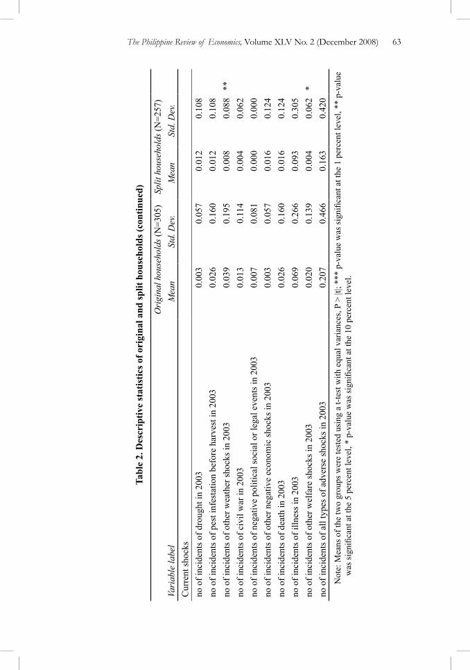
Because of the longer history of original households, it is expected that they report more incidents of adverse shocks occurring over the last twenty years compared to split households. On the other hand, there does not seem to be a significant difference between the experience of current shocks for original and split households, except for other weather shocks and other welfare shocks. Original households report a higher incidence of these two shocks during the year, which is plausible because of their greater involvement in farming and their demographic composition.
5. Empirical analysis
We conduct separate analysis for original versus split households for two reasons. First, because split households are formed by children of original households, the two groups are not independent, having shared common characteristics in the past. Second, the two groups of households are at different stages of their life cycle.8 Original households are expected to have an older
8In the Philippines, the process of setting up independent households by children is more of a life-cycle phenomenon rather than a choice variable. When the children marry, they typi-cally stay with their parents in the beginning and then later set up their own household.
The Philippine Review of Economics, volume XLv No. 2 (December 2008) 65
demographic composition compared to the split households, and each group may respond differently to adverse shocks.
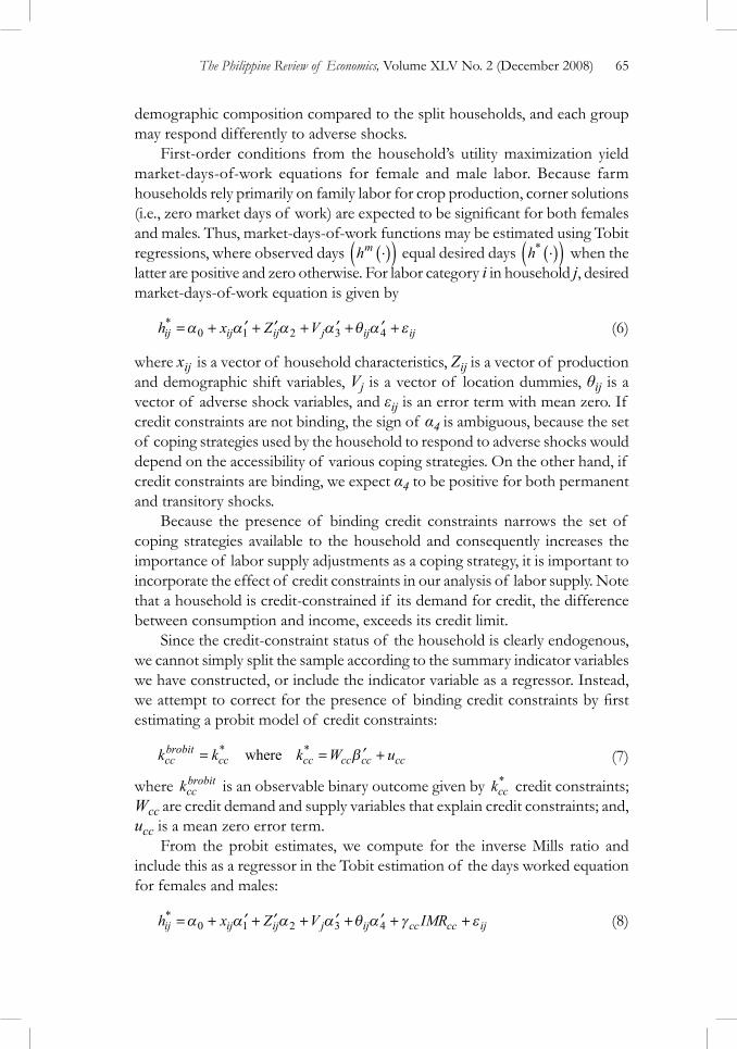
First-order conditions from the household’s utility maximization yield market-days-of-work equations for female and male labor. Because farm households rely primarily on family labor for crop production, corner solutions (i.e., zero market days of work) are expected to be significant for both females and males. Thus, market-days-of-work functions may be estimated using Tobit regressions, where observed days hm ⋅( )( ) equal desired days h* ⋅( )( ) when the latter are positive and zero otherwise. For labor category i in household j, desired market-days-of-work equation is given by
h x Z Vij ij ij j ij ij* = + ′ + ′ + ′ + ′ +α α α α θ α ε0 1 2 3 4 (6)
where xij is a vector of household characteristics, Zij is a vector of production and demographic shift variables, Vj is a vector of location dummies, θij is a vector of adverse shock variables, and εij is an error term with mean zero. If credit constraints are not binding, the sign of α4 is ambiguous, because the set of coping strategies used by the household to respond to adverse shocks would depend on the accessibility of various coping strategies. On the other hand, if credit constraints are binding, we expect α4 to be positive for both permanent and transitory shocks.
Because the presence of binding credit constraints narrows the set of coping strategies available to the household and consequently increases the importance of labor supply adjustments as a coping strategy, it is important to incorporate the effect of credit constraints in our analysis of labor supply. Note that a household is credit-constrained if its demand for credit, the difference between consumption and income, exceeds its credit limit.
Since the credit-constraint status of the household is clearly endogenous, we cannot simply split the sample according to the summary indicator variables we have constructed, or include the indicator variable as a regressor. Instead, we attempt to correct for the presence of binding credit constraints by first estimating a probit model of credit constraints:
k k k W uccbrobit
cc cc cc cc cc= = ′ +* *where β (7)
where kccbrobit is an observable binary outcome given by kcc
* credit constraints; Wcc are credit demand and supply variables that explain credit constraints; and, ucc is a mean zero error term.
From the probit estimates, we compute for the inverse Mills ratio and include this as a regressor in the Tobit estimation of the days worked equation for females and males:
h x Z V IMRij ij ij j ij cc cc ij* = + ′ + ′ + ′ + ′ + +α α α α θ α γ ε0 1 2 3 4 (8)
66 Malapit et al.: Labor supply adverse shocks and credit constraints
5.1. Market wage rates and crop profits
Because we are considering multiple-worker households, there is an empirical issue as to what is the relevant market wage for the household. The conventional approach to this problem is to take gender- and year-specific village average wages as the wage applicable to broad aggregates of household labor [Rose 1992; Skoufias 1994]. Kochar [1999] develops an alternative approach based on the observation that total labor hours in agriculture is the sum of hours spent in distinct agricultural tasks, with little variation across individuals performing the same task. Thus, wage rates for aggregate household labor can be calculated as the weighted average of village-year-gender and task-specific wages, with the share of household time devoted to specific tasks as weights.
However, Kochar [1999] also notes that since observed wages also reflect household decisions on how much time is spent on each activity, this measure will be endogenous and correlated with unobserved characteristics affecting market hours. Since our research objectives do not require an explicit measure of wages, we follow Kochar’s [1999] approach in substituting for market wages its exogenous determinants (primarily demographic variables) that determine the household’s choice of market activities.
The same approach is used in the treatment of crop profits. The use of instrumental variables techniques did not result in significant estimates for predicted profits in the Tobit estimation of days worked. As we noted earlier, however, crop profits may lead to biased estimates due to measurement errors and unobserved variables. Instead, we include the self-reported incidents of crop failure as regressors in the labor-supply estimation and omit crop profits as a regressor in favor of its exogenous determinants that determine production decisions. These include farm characteristics, household-head characteristics affecting farm productivity, demographic variables, and location dummies to account for price levels and level of economic activity.
6. Results
6.1. Credit constraint estimates
In our estimation of credit constraints, we include as regressors independent variables that influence either the demand or supply of credit (or both): household size, the dependency ratio, household head characteristics (ethnicity; age; age squared; highest grade attained), number of prime-age males and females, area of land cultivated, dummy variables for crop choice (sugar; corn; and rice), number of adverse shocks occurring before 2003, a dummy variable =1 if the household has borrowed at least once in the past year, and location dummies. Results of the probits for both original and split households are presented in Table 3.
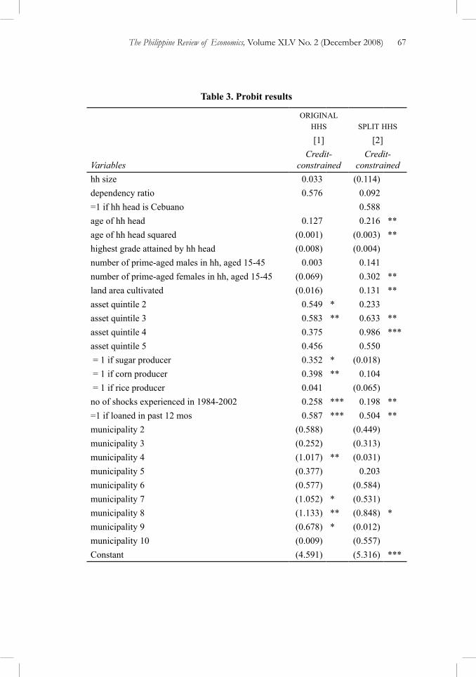
The Philippine Review of Economics, volume XLv No. 2 (December 2008) 67
Table 3. Probit results
original hhs split hhs
[1] [2]
VariablesCredit-
constrainedCredit-
constrainedhh size 0.033 (0.114)dependency ratio 0.576 0.092 =1 if hh head is Cebuano 0.588 age of hh head 0.127 0.216 **age of hh head squared (0.001) (0.003) **highest grade attained by hh head (0.008) (0.004)number of prime-aged males in hh, aged 15-45 0.003 0.141 number of prime-aged females in hh, aged 15-45 (0.069) 0.302 **land area cultivated (0.016) 0.131 **asset quintile 2 0.549 * 0.233 asset quintile 3 0.583 ** 0.633 **asset quintile 4 0.375 0.986 ***asset quintile 5 0.456 0.550 = 1 if sugar producer 0.352 * (0.018) = 1 if corn producer 0.398 ** 0.104 = 1 if rice producer 0.041 (0.065)no of shocks experienced in 1984-2002 0.258 *** 0.198 ** =1 if loaned in past 12 mos 0.587 *** 0.504 **municipality 2 (0.588) (0.449)municipality 3 (0.252) (0.313)municipality 4 (1.017) ** (0.031)municipality 5 (0.377) 0.203 municipality 6 (0.577) (0.584)municipality 7 (1.052) * (0.531)municipality 8 (1.133) ** (0.848) *municipality 9 (0.678) * (0.012)municipality 10 (0.009) (0.557)Constant (4.591) (5.316) ***
68 Malapit et al.: Labor supply adverse shocks and credit constraints
We find that original households involved in sugar production as well as corn production are more likely to be credit constrained. This may be explained by the higher working capital requirement of these crops (particularly sugar), relative to other crops (rice, vegetables, coconut, etc.). Also, original households belonging to the second and third asset quintiles are more likely to be credit constrained relative to those in the lowest quintile. This could be reflecting higher demand for credit if these households are able to operate their farms or family businesses at a larger scale than households with less assets.
In addition, original households are more likely to be credit constrained if they have already borrowed at least once in the past year. Having borrowed in the past year could indicate a draw on the household’s credit limit, so that additional demand for loans may no longer be accommodated in full.
Finally, original households are more likely to be credit constrained the more adverse shocks it has experienced in the last twenty years. This supports the view that persistent shocks have lasting effects on household welfare, since shocks occurring in the past continue to strongly influence current credit constraints.
As for the split households, we find that a number of household characteristics significantly explain the credit constraint status of the household. The household head’s age and age squared, and the number of prime-age males and females in the household all contribute to the probability that the household will be credit constrained. If the age of the household head captures experience and unobserved variables affecting productivity and creditworthiness, then this result is contrary to what we would expect. However, both the age and labor endowments of the household could be capturing the effect on demand for credit rather than supply, so that a household with more experience in farming, and more labor endowments may be operating at a larger scale and therefore would demand more working capital. We also find that split households with more land cultivated, and those belonging to the third and fourth asset quintiles are more likely to be credit constrained. This seems to fit into our explanation that households with more assets (land, prime-age workers, etc.) are more likely to be operating their farms or family businesses at a higher scale and would require more credit for working capital.
Similar to the findings for original households, a split household is also more likely to be credit constrained the more shocks it has experienced in the past, and if it has already borrowed in the past year. As we have noted above, this could simply be capturing a draw on the household’s credit limit.
The probit model for both subsamples performed relatively well in predicting the self-reported credit constraint status of households. The model correctly predicted the credit constraint status of 68 percent of the subsample of original households, and correctly predicted the credit constraint status of 74 percent of the subsample of split households.

The Philippine Review of Economics, volume XLv No. 2 (December 2008) 69
6.2. Labor supply responses
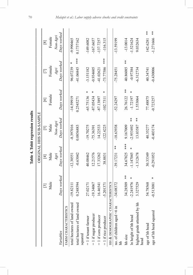
Our findings for the Tobit regressions are presented in Table 4 for original households, and Table 5 for the split households. We used days worked off-farm in the past year as the dependent variable, and ran separate regressions for total days worked, agricultural days worked, and non-agricultural days worked (where total days is the sum of agricultural and non-agricultural days worked) for males and females, and by household type.
We include the following independent variables as regressors: household characteristics (household size; number of young children; household head’s age, age squared, height, and highest grade attained; asset quintiles), production and demographic shift characteristics (area of land owned and its square; sugar, corn, or rice producer; number, mean age, and mean age squared of prime-age males and females; number of prime-age males and females with secondary and higher education), incidents of current shocks, location dummies, and the inverse Mills ratios computed from the corresponding probit regression. A summary of the signs of significant shock coefficients are presented in Table 6.
For original households, we find that males work more in agricultural off-farm jobs in response to droughts and other negative economic shocks, and work more in non-agricultural off-farm jobs in response to incidents of civil war/theft. This “added worker effect” for male workers is contrary to the hypothesis that male workers are already labor constrained and can no longer increase labor supplied. On the other hand, we find a “discouraged worker effect” for males in non-agricultural off-farm work in response to droughts as well. This result is unexpected because we expect weather shock such as a drought to affect the demand for agricultural workers rather than non-agricultural workers. Instead, we find the opposite here: male workers are able to work more in agricultural jobs, and work less in non-agricultural jobs in response to a drought. One possible explanation is that non-agricultural jobs may be strongly interlinked with agricultural activity (e.g., downstream services and industries such as transportation, food processing, etc.) so much so that it is more likely to suffer more when farm production is low.
On the other hand, we find that females in original households work less in both agricultural and non-agricultural off-farm jobs in response to droughts. Since we expect a sudden fall in agricultural activity during droughts, it is possible that there is some substitution between male and female workers, especially if male workers are the preferred type of labor for certain types of agricultural work.9 This observation is corroborated in the qualitative case studies conducted in our study area [Montillo-Burton 2005], where agricultural jobs are rationed to male workers during agricultural slack periods.
9For example, land preparation and hauling of sugarcane are male-dominated activities.
70 Malapit et al.: Labor supply adverse shocks and credit constraints
Tabl
e 4.
Tob
it re
gres
sion
res
ults
OR
IGIN
AL
HH
S SU
B-S
AM
PLE
[3]
[4]
[5]
[6]
[7]
[8]
Mal
eM
ale
Mal
eFe
mal
eFe
mal
eFe
mal
e
Vari
able
sD
ays w
orke
dAg
ri
Day
s wor
ked
Non
-Agr
i D
ays w
orke
dD
ays w
orke
dAg
ri
Day
s wor
ked
Non
-Agr
i D
ays w
orke
dfa
rm
ch
ar
ac
ter
isti
cs
tota
l hec
tare
s of l
and
owne
d-1
9.82
111
-12.
3055
1-8
.397
016
-14.
5991
996
.072
39*
-9.9
9046
5to
tal h
ecta
res o
f lan
d ow
ned
squa
red
0.24
8594
-0.6
3042
0.08
5688
30.
2545
271
-41.
0684
5**
*0.
1737
162
= 1
if te
nant
farm
er27
.021
7140
.084
62-1
9.70
275
-65.
7513
6*
-3.1
5118
2-1
49.6
082
= 1
if su
gar p
rodu
cer
-19.
3406
712
.215
76-7
5.36
391
-87.
0543
4*
-0.9
3460
5-1
67.6
657
= 1
if co
rn p
rodu
cer
16.4
6541
17.3
3262
14.2
2533
-87.
1389
7-4
1.02
621
-137
.725
7=
1 if
rice
prod
ucer
-5.2
0137
138
.883
1-1
22.4
225
-102
.731
1*
-73.
7758
6**
*-1
16.3
15h
h &
dem
og
ra
phic
ch
ar
ac
ter
isti
cs
no. o
f chi
ldre
n ag
ed <
6 in
hh
-34.
0837
2-3
9.17
231
**-1
8.63
938
-52.
2429
7-7
5.28
451
-13.
5919
9
hh si
ze34
.285
09**
34.6
7825
***
9.16
7009
26.7
6122
**40
.860
85**
-13.
0014
ln h
eigh
t of h
h he
ad-2
.241
976
*-1
.147
045
*-2
.953
492
**-1
.721
97*
-0.9
7384
-1.5
2162
4hi
ghes
t gra
de a
ttain
ed b
y hh
he
ad3.
3275
29-1
.312
678
13.0
3587
**1.
5530
64-6
.312
734
9.03
2634
age
of h
h he
ad54
.785
6830
.333
4940
.352
7777
.488
7540
.347
4114
2.62
81**
age
of h
h he
ad sq
uare
d-0
.513
081
*-0
.291
052
-0.4
0317
4-0
.723
257
-0.4
3000
6-1
.271
666
**

The Philippine Review of Economics, volume XLv No. 2 (December 2008) 71
Tabl
e 4.
Tob
it re
gres
sion
res
ults
(con
tinue
d)
OR
IGIN
AL
HH
S SU
B-S
AM
PLE
[3]
[4]
[5]
[6]
[7]
[8]
Mal
eM
ale
Mal
eFe
mal
eFe
mal
eFe
mal
e
Vari
able
sD
ays w
orke
dAg
ri
Day
s wor
ked
Non
-Agr
i D
ays w
orke
dD
ays w
orke
dAg
ri
Day
s wor
ked
Non
-Agr
i D
ays w
orke
dh
h &
dem
og
ra
phic
ch
ar
ac
ter
isti
cs
no. o
f prim
e-ag
ed m
ales
in
hh, a
ged
15-4
510
.129
4817
.967
78-1
7.85
001
-50.
5196
5**
-65.
1878
6**
*10
.671
65
no.
of p
rime-
aged
mal
es in
hh
, age
d 15
-45
-44.
9241
3*
-18.
5311
9-4
3.60
9925
.355
4717
.162
67-6
.374
309
ave
age
of m
ales
in h
h ag
ed
15-4
55.
6315
39-0
.338
417
.725
42**
*-0
.911
066
3.22
5557
-6.9
6532
3
ave
age
of m
ales
in h
h ag
ed
15-4
5 sq
uare
d-0
.048
664
0.03
2741
8-0
.290
351
*0.
0472
972
-0.0
4541
40.
1412
227
ave
age
of fe
mal
es in
hh
aged
15-
452.
2923
48-6
.119
447
**12
.747
2*
0.57
7548
1-0
.547
485
5.03
0414
ave
age
of fe
mal
es in
hh
aged
15-
45 sq
uare
d-0
.046
369
0.10
1285
6-0
.224
995
0.01
3714
30.
0021
655
0.00
0027
2
no. o
f mal
es in
hh
aged
15
-45
w/
seco
ndar
y ed
uc21
.278
09-9
.356
058
61.6
1928
***
0.56
3757
44.
7859
425.
1795
78no
. of m
ales
in h
h ag
ed
15-4
5 w
/

72 Malapit et al.: Labor supply adverse shocks and credit constraints
Tabl
e 4.
Tob
it re
gres
sion
res
ults
(con
tinue
d)
OR
IGIN
AL
HH
S SU
B-S
AM
PLE
[3]
[4]
[5]
[6]
[7]
[8]
Mal
eM
ale
Mal
eFe
mal
eFe
mal
eFe
mal
e
Vari
able
sD
ays w
orke
dAg
ri
Day
s wor
ked
Non
-Agr
i D
ays w
orke
dD
ays w
orke
dAg
ri
Day
s wor
ked
Non
-Agr
i D
ays w
orke
dh
h &
dem
og
ra
phic
ch
ar
ac
ter
isti
cs
high
er e
duc
-17.
9971
7-9
7.48
555
***
58.3
1235
20.2
4282
-20.
8337
242
.123
79no
. of f
emal
es in
hh
aged
15
-45
w/
seco
ndar
y ed
uc-0
.601
461
41.0
691
**-9
2.24
785
*14
.948
2110
.021
0463
.318
98no
. of f
emal
es in
hh
aged
15
-45
w/
high
er e
duc
10.5
6401
4.87
3723
11.8
2487
80.2
6862
**-1
7.19
359
167.
4544
*as
set q
uint
ile 2
71.8
2901
44.7
1893
82.6
8035
-45.
0788
492
.000
24-2
01.4
097
asse
t qui
ntile
3-3
2.83
404
-42.
1891
8-4
7.98
864
10.5
6761
95.4
9756
-106
.975
1as
set q
uint
ile 4
-38.
2614
1*
-35.
9147
8-3
4.79
469
-101
.684
721
.682
16-2
15.1
464
asse
t qui
ntile
52.
6230
71-3
1.07
871
53.0
058
56.7
5327
84.3
0721
-29.
9489
8in
cid
ents
of
cu
rr
ent
sho
ck
s
drou
ght
66.7
9087
283.
6188
***
-203
3.71
9**
*-1
036.
586
***
-703
.441
***
-116
1.60
8*
pest
infe
stat
ion
befo
re
harv
est
-3.2
1829
916
0.20
89-2
52.3
652
146.
6176
162.
6888
110.
7277
othe
r wea
ther
shoc
ks-1
63.4
204
***
-35.
9163
7-3
34.8
537
6.73
0351
14.9
5355
-46.
7604
6

The Philippine Review of Economics, volume XLv No. 2 (December 2008) 73
Tabl
e 4.
Tob
it re
gres
sion
res
ults
(con
tinue
d)
OR
IGIN
AL
HH
S SU
B-S
AM
PLE
[3]
[4]
[5]
[6]
[7]
[8]
Mal
eM
ale
Mal
eFe
mal
eFe
mal
eFe
mal
e
Vari
able
sD
ays w
orke
dAg
ri
Day
s wor
ked
Non
-Agr
i D
ays w
orke
dD
ays w
orke
dAg
ri
Day
s wor
ked
Non
-Agr
i D
ays w
orke
din
cid
ents
of
cu
rr
ent
sho
ck
s
othe
r neg
ativ
e ec
onom
ic
shoc
ks
158.
3343
252.
884
***
-12.
9584
915
9.27
221
9.56
29*
-122
8.87
**
civi
l war
/thef
t/ban
ditry
212.
9615
*34
.555
6832
1.91
71**
-33.
5567
8-5
9.67
185
-143
4.27
4**
*de
ath
of h
h m
embe
r-8
0.52
071
19.9
6498
-165
.052
7-8
5.73
303
-716
.936
4**
*-1
03.3
777
illne
ss o
f hh
mem
ber
-59.
6259
2-1
2.27
236
-117
.092
291
.504
6186
.838
7117
.778
39ot
her w
elfa
re sh
ocks
-2
5.35
975
93.9
9732
-261
.263
995
.197
2813
7.50
6592
.492
67lo
cat
ion
du
mm
ies
mun
icip
ality
217
1.19
4619
4.94
7928
.791
1499
.815
55-5
88.8
647
***
123.
1836
mun
icip
ality
316
3.83
72**
175.
4723
**10
.066
1915
9.54
11*
301.
0007
***
32.2
9829
mun
icip
ality
421
8.65
79**
190.
3034
*87
.297
4327
7.96
49**
*28
1.44
49**
225.
5737
mun
icip
ality
521
7.95
71**
128.
808
157.
285
121.
3408
193.
9701
24.9
6652
mun
icip
ality
616
2.24
1**
104.
1241
64.4
7589
111.
9476
174.
2539
**78
.352
46m
unic
ipal
ity 7
150.
0371
119.
1074
52.6
0569
314.
8276
-517
.555
***
374.
9556
*m
unic
ipal
ity 8
205.
8429
166.
0453
187.
2443
172.
6181
259.
543
***
50.2
5031
mun
icip
ality
926
3.78
24**
*20
8.62
75**
189.
0241
161.
7504
215.
8116
*12
2.94
66m
unic
ipal
ity 1
021
1.77
04*
77.2
2673
232.
5624
**14
2.24
0314
2.80
9210
3.95
57
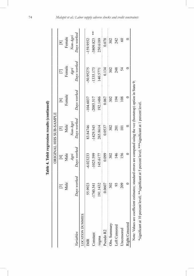
74 Malapit et al.: Labor supply adverse shocks and credit constraints
Tabl
e 4.
Tob
it re
gres
sion
res
ults
(con
tinue
d)
OR
IGIN
AL
HH
S SU
B-S
AM
PLE
[3]
[4]
[5]
[6]
[7]
[8]
Mal
eM
ale
Mal
eFe
mal
eFe
mal
eFe
mal
e
Vari
able
sD
ays w
orke
dAg
ri
Day
s wor
ked
Non
-Agr
i D
ays w
orke
dD
ays w
orke
dAg
ri
Day
s wor
ked
Non
-Agr
i D
ays w
orke
dlo
cat
ion
du
mm
ies
IMR
55.9
923
-6.0
2323
383
.847
46-1
04.6
037
-50.
9527
5-1
59.9
552
Con
stan
t-1
740.
541
-102
5.59
9-1
429.
545
-208
5.51
7-1
335.
173
-380
9.82
3**
/sig
ma
191.
1432
145.
6177
265.
8614
192.
1486
140.
5771
250.
6189
Pseu
do R
20.
0607
0.09
90.
0537
0.06
70.
134
0.07
8O
bs. S
umm
ary
302
302
302
302
302
302
Left
Cen
sore
d93
146
201
194
248
242
Unc
enso
red
209
156
101
108
5460
Rig
ht C
enso
red
00
00
00
Not
e: V
alue
s are
coe
ffici
ent e
stim
ates
; sta
ndar
d er
rors
are
com
pute
d us
ing
the
vce
(boo
tstra
p) o
ptio
n in
Sta
ta 9
;
*sig
nific
ant a
t 10
perc
ent l
evel
; **s
igni
fican
t at 5
per
cent
leve
l; **
*sig
nific
ant a
t 1 p
erce
nt le
vel.
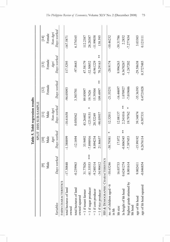
The Philippine Review of Economics, volume XLv No. 2 (December 2008) 75
Tabl
e 5.
Tob
it re
gres
sion
res
ults
SPLI
T H
HS
SUB
-SA
MPL
E[9
][1
0][1
1][1
2][1
3][1
4]M
ale
Mal
eM
ale
Fem
ale
Fem
ale
Fem
ale
Vari
able
sD
ays w
orke
dAg
ri
Day
s wor
ked
Non
-Agr
i D
ays w
orke
dD
ays w
orke
dAg
ri
Day
s wor
ked
Non
-Agr
i D
ays w
orke
dfa
rm
ch
ar
ac
ter
isti
cs
tota
l hec
tare
s of l
and
owne
d-1
7.30
848
-1.3
8889
9-1
8.61
658
-94.
0509
311
7.52
95-1
67.5
871
tota
l hec
tare
s of l
and
owne
d sq
uare
d-0
.239
963
-12.
1694
0.05
8562
3.30
3701
-97.
8643
6.37
4165
= 1
if te
nant
farm
er31
.770
2633
.949
243
.264
0289
.850
9747
.581
7911
2.23
87=
1 if
suga
r pro
duce
r-8
1.35
553
***
-7.8
9891
6-1
23.9
151
*19
.742
6-3
2.50
852
28.2
8387
= 1
if co
rn p
rodu
cer
-9.2
4831
48.
0942
3420
.522
4915
.393
04-0
.961
229
-11.
9903
8=
1 if
rice
prod
ucer
-34.
9041
221
.866
57-9
8.05
937
109.
4997
**70
.291
63**
138.
595
hh
& d
emo
gr
aph
ic c
ha
ra
cte
ris
tic
s
no. o
f chi
ldre
n ag
ed <
6 in
hh
-10.
6324
6-3
0.79
381
*12
.320
11-2
1.55
251
-20.
9174
-10.
4623
2
hh si
ze16
.037
3317
.072
12.0
8137
-16.
4469
79.
9962
63-3
9.31
786
ln h
eigh
t of h
h he
ad0.
6241
274
-0.8
0654
5**
2.24
1016
**1.
0709
270.
3670
267
2.28
52hi
ghes
t gra
de a
ttain
ed b
y hh
hea
d8.
0016
14-7
.397
453
19.7
9762
*-7
.019
686
-1.2
4720
2-7
.277
434
age
of h
h he
ad9.
0024
11-1
5.99
192
39.3
4874
-35.
3639
3-2
9.58
638
3.03
303
age
of h
h he
ad sq
uare
d-0
.046
854
0.26
7611
4-0
.507
331
0.47
2102
80.
3727
485
0.12
1111
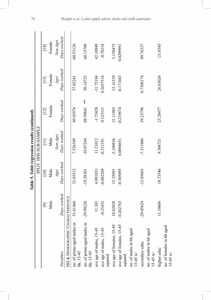
76 Malapit et al.: Labor supply adverse shocks and credit constraints
Tabl
e 5.
Tob
it re
gres
sion
res
ults
(con
tinue
d)
SPLI
T H
HS
SUB
-SA
MPL
E[9
][1
0][1
1][1
2][1
3][1
4]M
ale
Mal
eM
ale
Fem
ale
Fem
ale
Fem
ale
Vari
able
sD
ays w
orke
dAg
ri
Day
s wor
ked
Non
-Agr
i D
ays w
orke
dD
ays w
orke
dAg
ri
Day
s wor
ked
Non
-Agr
i D
ays w
orke
dh
h &
dem
og
ra
phic
ch
ar
ac
ter
isti
cs
no. o
f prim
e-ag
ed m
ales
in
hh, 1
5-45
51.6
1466
32.0
5512
7.52
6349
49.0
3976
37.8
2241
-60.
5312
6
no. o
f prim
e-ag
ed m
ales
in
hh, 1
5-45
-29.
9922
6-1
9.28
301
-10.
8724
488
.598
41**
50.1
4723
60.1
5708
ave
age
of m
ales
, 15-
4511
.383
4.09
1033
11.2
1012
-1.7
3428
-11.
7518
442
.109
49av
e ag
e of
mal
es, 1
5-45
sq
uare
d-0
.254
32-0
.082
209
-0.3
1219
10.
1231
110.
2657
514
-0.7
0218
ave
age
of fe
mal
es, 1
5-45
10.8
2038
15.2
5091
-2.1
0083
621
.119
8512
.163
393.
1584
75av
e ag
e of
fem
ales
, 15-
45
squa
red
-0.2
6276
5-0
.305
095
0.00
9465
1-0
.219
874
-0.1
7104
30.
0299
991
no. o
f mal
es in
hh
aged
15
-45
w/
seco
ndar
y ed
uc-2
9.05
624
-12.
8560
3-7
.513
486
39.2
3796
0.73
0817
489
.763
37no
. of m
ales
in h
h ag
ed
15-4
5 w
/ hi
gher
edu
c11
.106
0618
.735
469.
3067
2123
.284
7726
.030
26-2
1.03
45no
. of f
emal
es in
hh
aged
15
-45
w/
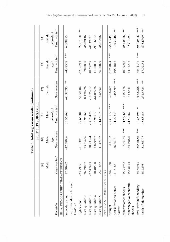
The Philippine Review of Economics, volume XLv No. 2 (December 2008) 77
Tabl
e 5.
Tob
it re
gres
sion
res
ults
(con
tinue
d)
SPLI
T H
HS
SUB
-SA
MPL
E[9
][1
0][1
1][1
2][1
3][1
4]M
ale
Mal
eM
ale
Fem
ale
Fem
ale
Fem
ale
Vari
able
sD
ays w
orke
dAg
ri
Day
s wor
ked
Non
-Agr
i D
ays w
orke
dD
ays w
orke
dAg
ri
Day
s wor
ked
Non
-Agr
i D
ays w
orke
dh
h &
dem
og
ra
phic
ch
ar
ac
ter
isti
cs
seco
ndar
y ed
uc17
.304
92-1
2.38
006
33.5
6868
-43.
3269
5**
-43.
8508
***
6.30
8755
no. o
f fem
ales
in h
h ag
ed
15-4
5 w
/ hi
gher
edu
c-2
3.79
791
-51.
8396
122
.655
0458
.590
04-6
2.36
213
228.
7318
**as
set q
uint
ile 2
26.3
9867
23.3
5456
18.9
5168
8.17
8726
28.0
808
46.0
9136
asse
t qui
ntile
3-2
.547
423
30.2
3394
-34.
2042
6-1
8.75
912
40.5
9257
-48.
3987
7as
set q
uint
ile 4
10.4
0508
3.87
9937
15.9
8717
-64.
0977
611
.080
31-9
3.16
812
asse
t qui
ntile
5-5
2.18
5211
.421
82-1
14.5
015
*16
.656
6156
.000
2946
.635
06in
cid
ents
of
cu
rr
ent
sho
ck
s
drou
ght
-247
.133
8-1
3.70
2-1
431.
177
***
-76.
6769
-319
.707
4**
*-5
6.31
745
pest
infe
stat
ion
befo
re
harv
est
-51.
5183
1-5
6.36
781
71.2
7333
-455
.99
***
-495
.181
5-9
43.9
48**
othe
r wea
ther
shoc
ks-5
5.93
982
70.5
385
***
-129
9.68
***
115.
476
107.
9218
-854
.066
6**
othe
r neg
ativ
e ec
onom
ic
shoc
ks
-156
.817
4-8
4.49
096
-217
.218
714
5.88
41-4
4.33
203
189.
3385
civi
l war
/thef
t/ban
ditry
24.6
5913
-555
.665
6**
*10
3.53
96*
-718
.896
8**
*-3
54.4
337
***
-980
.081
6**
*de
ath
of h
h m
embe
r-2
5.72
951
53.5
6707
-152
.815
623
3.58
24**
-17.
7935
457
5.63
09**

78 Malapit et al.: Labor supply adverse shocks and credit constraints
Tabl
e 5.
Tob
it re
gres
sion
res
ults
(con
tinue
d)SP
LIT
HH
S SU
B-S
AM
PLE
[9]
[10]
[11]
[12]
[13]
[14]
Mal
eM
ale
Mal
eFe
mal
eFe
mal
eFe
mal
e
Vari
able
sD
ays w
orke
dAg
ri
Day
s wor
ked
Non
-Agr
i D
ays w
orke
dD
ays w
orke
dAg
ri
Day
s wor
ked
Non
-Agr
i D
ays w
orke
din
cid
ents
of
cu
rr
ent
sho
ck
s
illne
ss o
f hh
mem
ber
-37.
6060
3*
-61.
1057
4**
-26.
1279
9-6
2.49
477
-52.
3625
8-4
7.44
997
othe
r wel
fare
shoc
ks
119.
7216
**-5
45.8
62**
*17
1.34
32*
-798
.593
1**
*-3
45.1
45**
*-1
267.
006
***
loc
atio
n d
um
mie
s
mun
icip
ality
238
.128
1760
.557
39-4
3.96
792
-65.
1765
3-5
0.85
257
-61.
2082
8m
unic
ipal
ity 3
27.0
4538
123.
967
-93.
1129
-6.3
2767
75.6
8089
-84.
7341
3m
unic
ipal
ity 4
38.0
0442
118.
5623
-57.
8872
5-8
5.80
656
46.4
565
-300
.934
5m
unic
ipal
ity 5
39.8
6607
40.6
3795
-15.
8929
-51.
6345
5-3
1.82
712
-91.
6891
6m
unic
ipal
ity 6
26.7
1459
36.5
9702
16.6
4724
-2.2
5808
84.
0704
4264
.179
42m
unic
ipal
ity 7
73.4
3937
128.
9719
-64.
8648
327
.318
94-3
49.8
93**
*76
.859
71m
unic
ipal
ity 8
78.1
2214
160.
8914
-71.
0768
380
.558
8889
.409
910.
4914
025
mun
icip
ality
944
.497
8210
5.79
35-2
1.19
424
-70.
4408
825
.188
66-2
22.9
989
*m
unic
ipal
ity 1
032
.835
0372
.148
47-4
8.50
911
-28.
1452
648
.356
51-6
6.98
906
IMR
-9.4
4680
9-3
1.05
987
30.4
3579
-22.
0830
3-2
4.60
56-2
2.61
184
Con
stan
t-4
96.8
119
-12.
9628
1-1
053.
557
*5.
6700
5920
3.31
94-1
125.
047
/sig
ma
129.
5758
93.4
2272
204.
0346
142.
7289
74.0
0282
222.
3158

The Philippine Review of Economics, volume XLv No. 2 (December 2008) 79
Tabl
e 5.
Tob
it re
gres
sion
res
ults
(con
tinue
d)SP
LIT
HH
S SU
B-S
AM
PLE
[9]
[10]
[11]
[12]
[13]
[14]
Mal
eM
ale
Mal
eFe
mal
eFe
mal
eFe
mal
e
Vari
able
sD
ays w
orke
dAg
ri
Day
s wor
ked
Non
-Agr
i D
ays w
orke
dD
ays w
orke
dAg
ri
Day
s wor
ked
Non
-Agr
i D
ays w
orke
dPs
eudo
R2
0.03
80.
0803
0.03
90.
0792
0.15
30.
1147
Obs
. sum
mar
y25
625
625
625
625
625
6Le
ft ce
nsor
ed38
130
127
171
204
219
Unc
enso
red
218
126
129
8552
37R
ight
cen
sore
d0
00
00
0
Not
e: V
alue
s are
coe
ffici
ent e
stim
ates
; sta
ndar
d er
rors
are
com
pute
d us
ing
the
vce(
boot
stra
p) o
ptio
n in
Sta
ta 9
;
*sig
nific
ant a
t 10
perc
ent l
evel
; **s
igni
fican
t at 5
per
cent
leve
l; **
*sig
nific
ant a
t 1 p
erce
nt le
vel.
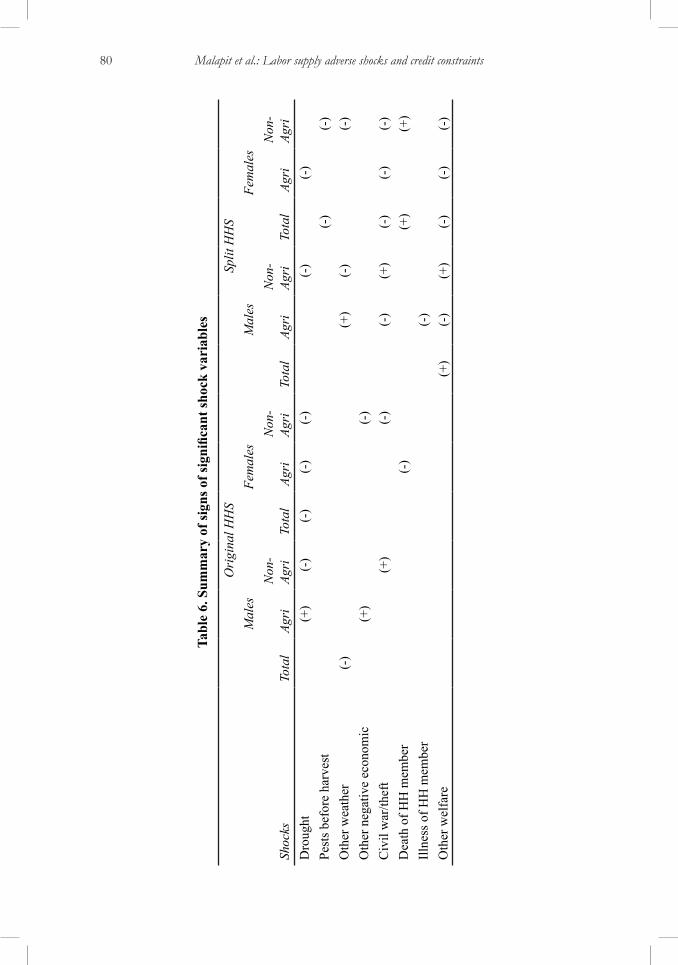
80 Malapit et al.: Labor supply adverse shocks and credit constraints
Tabl
e 6.
Sum
mar
y of
sign
s of s
igni
fican
t sho
ck v
aria
bles
Ori
gina
l HH
SSp
lit H
HS
Mal
esFe
mal
esM
ales
Fem
ales
Shoc
ksTo
tal
Agri
Non
-Ag
riTo
tal
Agri
Non
-Ag
riTo
tal
Agri
Non
-Ag
riTo
tal
Agri
Non
-Ag
riD
roug
ht(+
)(-
)(-
)(-
)(-
)(-
)(-
)Pe
sts b
efor
e ha
rves
t(-
)(-
)O
ther
wea
ther
(-)
(+)
(-)
(-)
Oth
er n
egat
ive
econ
omic
(+)
(-)
Civ
il w
ar/th
eft
(+)
(-)
(-)
(+)
(-)
(-)
(-)
Dea
th o
f HH
mem
ber
(-)
(+)
(+)
Illne
ss o
f HH
mem
ber
(-)
Oth
er w
elfa
re(+
)(-
)(+
)(-
)(-
)(-
)
The Philippine Review of Economics, volume XLv No. 2 (December 2008) 81
Females in original households also work less days in non-agricultural off-farm jobs in response to other negative economic shocks, incidents of civil war/theft, and work less days in agricultural jobs in response to deaths of household members. This result could be reflecting a reallocation of men and women’s time between off-farm work, and own-farm and domestic work. Note that for other negative economic shocks and civil war/theft, males are able to increase days worked off-farm, but women decrease days worked off-farm. If either males are more valuable in the labor market or there are other barriers to the participation of women in the labor market, it is possible that in the event of such types of shocks, men are tasked to increase income through wages while women take over more tasks at home and in their own farms.
In the case of split households, we find that the various environmental shocks (drought, pests, and other weather) almost always result in a decrease in off-farm days worked for both males and females, except for other weather shocks where males are able to increase days worked in agricultural jobs. We also find that males work less in agricultural off-farm jobs but work more in non-agricultural off-farm jobs in response to incidents of civil war/theft and other welfare shocks. Females, on the other hand, work less in both agricultural and non-agricultural off-farm jobs in response to both types of shocks.
Finally, we find that females in split households increase days worked in non-agricultural jobs in response to incidents of death in the household, while males decrease agricultural days worked off-farm in response to illness. Both these results are within our expectations. If the household member who died was of prime working age, then the response of females could be interpreted as truly an “added worker effect” where they attempt to replace the lost income by working off-farm in non-agricultural jobs. On the other hand, if the household member who died is a child or an elderly member, then this may actually reduce the domestic responsibilities of women at home so that they are now able to work off-farm. In the case of illness, this is a type of shock that temporarily reduces the endowment of labor (especially if it is the male members who fell ill), so it is not surprising that males work less in response to it.
Comparing the two subsamples, we note that while male workers seem to perform the “added worker” function in original households, both males and females are able to do so in split households. In particular, since split households are better educated, on average, than their parent households, it appears they are better able to increase labor supplied to non-agricultural work for both males and females. Also, while environmental shocks appear to be highly important for both groups in explaining days worked off-farm, split households seem to be more vulnerable as they respond to a larger variety of shocks compared to original households.
Lastly, none of the coefficients for the inverse Mills ratios were significant. This implies that the household’s credit-constraint status does not influence

82 Malapit et al.: Labor supply adverse shocks and credit constraints
the household’s off-farm labor decisions. This casts some doubt on the hypothesis that households smooth consumption primarily through credit because households that were not credit constrained need not resort to labor-supply adjustments in response to adverse shocks. Instead, our results suggest that households resort to labor supply adjustments independently of their ability to borrow. In fact, the converse may be true: households may borrow in response to an adverse shock only when they are unable to raise the additional funds through wages. Whether or not this is indeed the case requires further investigation, although this observation is in line with Kochar’s [1995] argument that well-functioning labor markets reduce the need to resort to asset depletion and other costly ex ante measures.
7. Summary and conclusion
We find that males and females respond differently to different types of adverse shocks. For both original and split households, we find evidence for labor-demand constraints in both agricultural and non-agricultural off-farm jobs in response to environmental shocks, although males seem to be able to overcome such labor constraints. If either males are more valuable in the labor market or there are barriers to women’s participation in the labor market, women may be unable to maintain, much less increase, labor supplied off-farm because the limited opportunities (due to the aggregate weather shock) are rationed to men.
Also, we find that only males are able to work more off-farm in response to shocks in original households, while both males and females are able to increase off-farm work in response to adverse shocks in split households. We attribute this difference to the higher average educational attainment of split households compared to that of their parents, thus enabling them to better access non-agricultural jobs off-farm. In particular, higher education for females was highly significant in explaining days worked in non-agricultural jobs for both original and split households.
None of the coefficients for the inverse Mills ratios were significant in explaining off-farm labor supply, casting doubt on the hypothesis that households smooth consumption primarily through credit. Our results suggest that households resort to labor-supply adjustments independently of their ability to borrow, which is in line with Kochar’s [1995] argument that well-functioning labor markets reduce the need to resort to asset depletion and other costly ex ante measures.
Although an evaluation of the effectiveness of these labor adjustment strategies is beyond the scope of this paper, it is clear that households that are disadvantaged with respect to the quality and quantity of their labor endowments are least likely to cope well with adverse shocks. Our results suggest that the
The Philippine Review of Economics, volume XLv No. 2 (December 2008) 83
most vulnerable households are those with little education and with few or no able-bodied male members.
Adverse environmental shocks in particular appear to be one of the most serious shocks faced by households. It is even worse for households with few males because as we noted, female labor-supply response to these shocks is always negative for both original and split households. Clearly, there is an opportunity for countercyclical workfare programs to improve the welfare of vulnerable households in this case. Such a program could be designed to target households unable to use labor markets to compensate for lost incomes, i.e., households with high female-to-male ratios, households with high dependency ratios, and households with little or no education.
In addition to workfare programs during periods of adverse weather, a medium- to long-run policy response is the provision of universal education and health care. These programs are likely to be effective in strengthening the labor endowments of households and improving their ability to cope with adverse shocks in the future.
Finally, further investigation is necessary to explain the barriers to women’s participation in labor markets or other such institutional constraints, especially in light of weather shocks. Qualitative and anthropological approaches may be particularly useful in identifying more specific and effective ways to ease the labor constraint for women.

84 Malapit et al.: Labor supply adverse shocks and credit constraints
References
Ashenfelter, O. [1980] “Unemployment as disequilibrium in a model of aggregate labor supply”, Econometrica 48(3): 547-564
Baslevent, C. and O. Onaran [2001] “Labor force participation of married couples in Turkey: analysis of the effect of export-oriented growth and added vs. discouraged worker effects”, Draft report for the Economic Research Forum (ERF) for Arab countries, Iran and Turkey.
Bouis, H. E. and L. J. Haddad [1990] Agricultural commercialization, nutrition and the rural poor: a study of Philippine farm households. Boulder and London: Lynne Riener.
Carter, M. R. and F. J. Zimmerman [2000] “The dynamic cost and persistence of asset inequality in an agrarian economy”, Journal of Development Economics 62: 265-302.
Coile, C. [2004] “Health shocks and couples’ labor supply decisions”, nber Working Paper No. 10810.
Cochrane, J. H. [1991] “A simple test of consumption insurance”, The Journal of Political Economy 99(5): 957-976.
Cullen, J. B. and J. Gruber [1996] “Spousal labor supply as insurance: does unemployment insurance crowd out the added worker effect?” nber Working Paper No. 5608.
Deaton, A. [1991] “Saving and liquidity constraints”, Econometrica 59: 1221-1248.Dehejia, R. and R. Gatti [2002] “Child labor: the role of income variability and
access to credit across countries”, nber Working Paper No. 9018.Dercon, S. [2001] “Assessing vulnerability to poverty”, Paper prepared for DfID.Engen, E. and J. Gruber (2001) “Unemployment insurance and precautionary
saving”, Journal of Monetary Economics 47(3): 545-579.Eswaran, M. and A. Kotwal [1986] “Access to capital and agrarian production
organization”, The Economic Journal 95(382): 492-498.Finegan, T. and R. Margo [1994] “Work relief and the labor force participation of
married women in 1940”, The Journal of Economic History 54(1): 64-84.García-Escribano, M. [2003] “Does spousal labor smooth fluctuations in husband’s
earnings? The role of liquidity constraints”, Ph.D. diss., University of Chicago.
Heckman, J., and T. MaCurdy [1980] “A life cycle model of female labour supply”, The Review of Economic Studies 47(1): 47-74.
Jacoby, H. and E. Skoufias [1997] “Risk, financial markets and human capital in a developing country”, Review of Economics and Statistics 64: 311-335.
Kochar, A. [1995] “Explaining household vulnerability to idiosyncratic income shocks,” American Economic Review 85(2): 159-164.

The Philippine Review of Economics, volume XLv No. 2 (December 2008) 85
Kochar, A. [1999] “Smoothing consumption by smoothing income: hours-of-work responses to idiosyncratic agricultural shocks in rural India”, Review of Economics and Statistics 81(1): 50-61.
Lim, J. [2000] “The effects of the East Asian crisis on the employment of women and men: the Philippine case”, World Development 28(7): 1285-1306.
Low, H. [1999] “Self insurance and unemployment benefit in a life-cycle model of labour supply and savings”, Institute for Fiscal Studies Working Paper No. W98/24.
Lundberg, S. [1985] “The added worker effect”, Journal of Labor Economic 3(1): 11-37.
Malapit, H. J. [2003] “Review of literature on the ‘added worker effect’,” Unpublished manuscript.
Maloney, T. [1991] “Unobserved variables and the elusive added worker effect”, Economica 58(230): 173-187.
Merrigan, P. and M. Normandin [1996] “Precautionary saving motives: an assessment from uk time series of cross- sections”, The Economic Journal 106(438): 1193-1208.
Mincer, J. [1962] “Labor force participation of married women: a study of labor supply” in: Aspects of Labor Economics. Princeton, N.J.: Princeton University Press.
Montillo-Burton, L., ed. [2005] “Bukidnon case studies”, Unpublished draft.Morduch, J. [1995]. “Income smoothing and consumption smoothing”, Journal of
Economics Perspectives 9(Summer): 103-114.Prieto-Rodriguez, J. and C. Rodriguez-Gutierrez [2000] “Participation of married
women in the labor market and the “added worker effect” in Europe”, iriss Working Paper Series No. 2000-12.
Rose, E. [1992] “Ex ante and ex post labor supply responses to risk in a low income area,” Manuscript, University of Washington.
Serneels, P. [2002] “The added worker effect and intrahousehold aspects of unemployment”, csae wps/2002-14.
Skoufias, E. [1994] “Intertemporal substitution in labor supply: micro evidence from rural India”, Working Paper No. WP-94-7, University of Colorado at Boulder, Institute of Behavioral Science, Population Program.
Skoufias, E. and A. R. Quisumbing [2002] “Consumption insurance and vulnerability to poverty: a synthesis of the evidence from Bangladesh, Ethiopia, Mali, Mexico and Russia”, Unpublished manuscript.
Stephens, M. Jr. [2001] “Worker displacement and the added worker effect”, nber Working Paper No. 8260.
Townsend, R. [1995] “Consumption insurance: an evaluation of risk-bearing systems in low-income economies”, Journal of Economic Perspectives 9(3): 83-102.

86 Malapit et al.: Labor supply adverse shocks and credit constraints
Zeldes, S. [1989] “Consumption and liquidity constraints: an empirical investigation”, Journal of Political Economy 97(2): 305-346.