the panel purchasing power parity puzzledpapell/puzzle.pdfwe call these findings the “panel...

The Panel Purchasing Power Parity Puzzle

David H. Papell

Department of Economics University of Houston

Houston, TX 77204-5882 (713) 743-3807

E-Mail: [email protected]

April 2004

I am grateful to Charles Engel, Lutz Kilian, Chris Murray, Elena Pesavento, Helen Popper, Ken West, two anonymous referees, and to participants in seminars at Duke, Santa Cruz, Vanderbilt, Texas Econometrics Camp VI, and the 2002 International Economics and Finance Society meetings for helpful comments and discussions. I thank the National Science Foundation for financial support.

Does long-run purchasing power parity hold over the post-1973 floating exchange rate period? Panel unit root tests provide evidence of PPP that increases with the number of observations. The strengthening of the evidence, however, is highly cyclical. When the dollar appreciates at the end of the sample, the evidence of PPP strengthens and, when it depreciates, the evidence weakens. While these patterns cannot be explained by the specifications that are normally used to model real exchange rates, the strengthening, but not the cyclical pattern, can be explained by a specification that incorporates PPP restricted structural change.

1

1. Introduction

The behavior of real exchange rates over the post-1973 floating exchange rate period is one of the

most extensively studied empirical topics in international economics. The most frequently asked question

is whether long-run purchasing power parity holds over this period, posed statistically as whether unit

roots in real exchange rates can be rejected. Despite the large amount of research on this topic, we do not

have a definitive answer to the most basic issues. Is the real exchange rate mean reverting, or does it have

a unit root? If it is mean reverting, what is the process of adjustment to the mean?

Much of this work has been inspired by the development of panel unit root tests, which exploit

cross-section as well as time series variability in an attempt to increase power over univariate methods.

Although Frankel and Rose (1996), in an article that has served as a catalyst to much subsequent research,

found strong evidence of PPP, panel methods have not provided an unequivocal answer. Unit roots in

real exchange rates are at best marginally rejected using panels of quarterly data when, as in Papell

(1997), serial correlation is emphasized and the U.S. dollar is used as the numeraire currency or, as in

O'Connell (1998), contemporaneous correlation is accounted for and methods are used which render the

numeraire irrelevant.1

Recent work has begun to appear which reports strong rejections of unit roots in real exchange

rates for panels with quarterly data. Wu and Wu (2001), extending the tests of Im, Pesaran and Shin

(1996) and Maddala and Wu (1999) to allow for contemporaneous correlation, report strong rejections for

panels of industrialized countries with both the U.S. dollar and the German mark as numeraire. Higgins

and Zakrajsek (1999), using several panel methods with both CPI and WPI based real exchange rates,

report very strong unit root rejections for panels of economically open, OECD, and European countries

with the U.S. dollar as numeraire.

The strong rejections of unit roots in real exchange rates comes from research that exhibits

substantial variety in the composition of the panels and in the estimation techniques. A common element,

however, is that the data extends through 1997. The starting point of the paper is to document how the

evidence against unit roots in real exchange rates, and thus evidence of PPP, substantially increases as

observations for 1997 and 1998 are included in the data. We conduct unit root tests for panels of 20 real

exchange rates, constructed from nominal exchange rates and consumer price indexes of 21 industrialized

countries, with the United States dollar as the numeraire currency. Our estimation method, described in

detail below, allows for both contemporaneous correlation and heterogeneous serial correlation.

1 The unit root null is consistently rejected for panels of CPI based real exchange rates of European or industrialized countries when the German mark or other European currencies are used as the numeraire. See Jorion and Sweeney (1996), Papell (1997), and Papell and Theodoridis (2001).

2

We first conduct unit root tests on quarterly data that spans from 1973(1) to 1988(1). We then

add observations quarter-by-quarter, ending in 1998(4) when exchange rates among the Euro countries

became irrevocably fixed. This produces a series of 44 t-statistics. Since the distributions of the panel

unit root tests are non-standard, we use monte carlo methods to calculate critical values which reflect the

size of the panel, the number of observations, and the pattern of contemporaneous correlation in the actual

data. We confirm that the evidence against unit roots in real exchange rates increases with the number of

observations and strengthens dramatically as the end of the data extends past 1996. The strengthening of

the evidence, however, cannot be explained solely by the longer span of the data. In addition, the

evidence of PPP is highly cyclical and related to the value of the real exchange rate at the end of the

sample. When the dollar appreciates, the evidence of PPP strengthens and, when it depreciates, the

evidence weakens. We call these findings the “panel purchasing power parity puzzle.”2

We turn our attention towards finding an explanation for this puzzle. Using simulation methods,

we artificially generate a variety of panels of "real exchange rates" which match the dimensions and

replicate the pattern of contemporaneous correlation of the actual data. We then conduct panel unit root

tests on the artificial data, starting with the first 61 observations (corresponding to the initial 1973(1) -

1988(1) sample), and adding observations one at a time until all 104 observations in the 1973(1) - 1998(4)

sample are used. Finally, we compare the "evidence" of PPP found in the actual and simulated data over

the 44 sample lengths.

Suppose the real exchange rate is specified as a first-order autoregressive process, where the

variable is regressed on a constant and one lagged level. If the coefficient on the lagged level is below

one, the real exchange rate is stationary and PPP holds. If the coefficient equals one, the real exchange

rate has a unit root and PPP does not hold. We first generate artificial real exchange rates that have a unit

root. This is clearly a poor specification, as the unit root null is rejected far more strongly in the actual

than in the simulated data. We then generate artificial data that are stationary. While the congruence

between the results with actual and simulated data improves, the simulated data cannot replicate either the

strengthening or the cyclical pattern found in the results with the actual data.

Engel (2000) argues that, because of size distortions, the unit root null may be inappropriately

rejected in long-horizon data. He specifies a specification of the real exchange rate that is a combination

of a stationary and a unit root process, with the innovation variance of the former much larger than the

latter. Although this specification contains a permanent component, the unit root null is rejected over

90% of the time. Engel conjectures that the same size distortions would apply to panel tests. We

2 The cyclical evidence appears to be specific to dollar-based real exchange rates. Lopez and Papell (2003) find strengthening evidence of PPP for panels when European currencies are used as the numeraire following the Maastricht Treaty and with the advent of the Euro.

3

construct panels using Engel's specification, and confirm his conjecture. The unit root null is rejected at

the 5% level for each of the 44 sample lengths.

This evidence, however, is too strong. The artificial data provides much stronger evidence of

PPP than the actual data. If real exchange rates were truly generated according to Engel's specification,

we should have seen strong rejections of unit roots using panel methods for samples ending in 1988 and

later, not in 1997 and later. By raising the size of the coefficient on the lagged real exchange rate in the

stationary part of Engel's specification, the congruence between the results with actual and simulated data

can be improved. The strengthening and cyclical patterns, however, cannot be replicated. The fit is

similar to that obtained using the stationary specification above, which is simply an example of near

observational equivalence between stationary and non-stationary representations.

The possibility of nonlinear adjustment to PPP has received considerable recent attention. One

specification, used by Obstfeld and Taylor (1997) and Taylor (2001), is that transactions costs lead to a

"band of inaction" within which real exchange rates follow a random walk. Outside the band, there is

linear reversion to the edge of the band. This can be modeled by a symmetric two-regime threshold

autoregression (TAR). We generate data according to the TAR specification, choosing values of the

threshold and speed of reversion to maximize the congruence between the results with actual and

simulated data. The fit is worse than that obtained using either the stationary or Engel's specification, and

the strengthening and cyclical patterns found in the actual data cannot be replicated.

Another characterization of nonlinear mean reversion, used by Taylor, Peel, and Sarno (2001),

uses proportional transactions costs to motivate smooth, rather than discrete, adjustment to PPP. They

specify an exponential smooth transition autoregressive (ESTAR) model, where the speed of adjustment

is related to the deviation from parity. We generate data according to the ESTAR specification, choosing

values of parameters and variances to maximize the congruence between the results with actual and

simulated data. The fit is indistinguishable from the fit of the TAR model, and therefore worse than that

obtained using either the stationary or Engel's specification. The strengthening and cyclical patterns

found in the actual data are not replicated.

Why would the strength of the evidence of PPP be positively related to the strength of the dollar

at the end of the sample? If anything, one would expect that stronger evidence of PPP would be found if

the end of the sample corresponded with the dollar at its median level. The answer, we conjecture,

involves the difference between the median level of the dollar between 1973 and 1998 and the median

level between 1988 and 1998. The large appreciation and depreciation of the dollar from 1980 to 1987

causes the median for the full sample to be considerably higher than the median for the 1988 - 1998

period. The difference is substantial enough so that every appreciation between 1988 and 1998 actually

represents a movement towards the 1973 - 1998 median.

4

We implement this conjecture by generating artificial data that, while consistent with long-run

PPP, incorporates the rise and fall of the dollar from 1980 to 1987. In Papell (2002), we show that panel

unit root tests which incorporate PPP restricted structural change provide much stronger evidence against

unit roots in real exchange rates than conventional panel unit root tests for those countries that adhere to

the "typical" pattern of the rise and fall of the dollar. The specification allows for three changes in the

slope of the deterministic component, but is restricted to return to its PPP value following the third break.

We choose the break dates by using the method of Bai (1999) with the average dollar real exchange rate

series. This specification better captures the strengthening of evidence for PPP as the sample lengthens

than the purely stationary, mixed stationary and unit root, or nonlinear mean reverting specifications

described above, and so the congruence between the results with artificial and simulated data improves.

The cyclical pattern found in the actual data, however, remains largely unexplained.

2. Panel Unit Root Tests of PPP

Purchasing power parity (PPP) is the hypothesis that the real exchange rate displays long-run

mean reversion. The real (dollar) exchange rate is calculated as follows,

ppeq −+= * , (1)

where q is the logarithm of the real exchange rate, e is the logarithm of the nominal (dollar) exchange

rate, p is the logarithm of the domestic CPI, and p* is the logarithm of the U.S. CPI.

2.1 Unit root tests

The most common test for PPP is the univariate Augmented-Dickey-Fuller (ADF) test, which

regresses the first difference of a variable (in this case the logarithm of the real exchange rate) on a

constant, its lagged level and k lagged first differences,

t

k

iiti qcqq

ttεαµ +∆++=∆ ∑

=−−

11

, (2)

A time trend is not included in equation (2) because such an inclusion would be theoretically inconsistent

with long-run PPP. The null hypothesis of a unit root is rejected in favor of the alternative of level

stationarity if α is significantly less than zero. Rejection of the unit root null provides evidence of mean

reversion and, hence, PPP. These tests provide very little evidence against unit roots for post-1973 real

exchange rates.

The low power of unit root tests against highly persistent alternatives with anything less than a

century of data has inspired the development of panel unit root tests which exploit cross section, as well

as time series, variation. Variants of these tests have been developed by Levin, Lin, and Chu (2002), Im,

Pesaran, and Shin (2003), Maddala and Wu (1999), and Bowman (1999). Applications of these tests to

post-1973 real exchange rates of industrialized countries include Abuaf and Jorion (1990), Frankel and

5

Rose (1996), Jorion and Sweeney (1996), Oh (1996), Wu (1996), Papell (1997), O’Connell (1998), Papell

and Theodoridis (1998,2001), Higgins and Zakrajsek (1999), and Wu and Wu (2001).

A panel extension of the univariate ADF test in Equation (2), which accounts for both a

heterogeneous intercept and serial correlation, would involve estimating the following equations,

jt

k

iijtijjtjjt qcqq εαµ +∆++=∆ ∑

=−−

11 , (3)

where the subscript j indexes the countries, and µj denotes the heterogeneous intercept. The test statistic

is the t-statistic on α. The null hypothesis is that all of the series contain a unit root and the alternative

hypothesis is that all of the series are stationary. In Papell (1997) and Papell and Theodoridis (2001), we

estimate Equation (3) using feasible GLS (seemingly unrelated regressions), with α equated across

countries and the values for k taken from the results of univariate ADF tests.3 For quarterly data with a

panel of 20 industrialized countries, we could not reject the unit root null at the 10 percent level with the

U.S. dollar as the numeraire currency.

2.2 Evidence of PPP as the span of the data increases

We first conduct unit root tests on quarterly data that spans from 1973(1) to 1988(1). We then

add observations quarter-by-quarter, ending in 1998(4) when exchange rates among the Euro countries

became irrevocably fixed. Since the distributions of the panel unit root tests are non-standard, we use

Monte Carlo methods to calculate critical values which reflect both the size of the panel and the exact

number of observations. For each span of the data, we fit univariate autoregressive (AR) models to the

first differences of the 20 real exchange rates, treat the optimal estimated AR models as the true data

generating processes for the errors in each of the series, and construct real exchange rate innovations from

the residuals. We then calculate the covariance matrix Σ of the innovations and use the optimal AR

models with iid N(0,Σ) innovations to construct pseudo samples of size equal to the actual size of our

series (64 to 104 observations). Since Σ is not diagonal, this preserves the cross-sectional dependence

found in the data. We then take partial sums so that the generated real exchange rates have a unit root by

construction.

We proceed to perform the estimation procedure described above on the generated data. For each

span of the data, we first estimate univariate ADF models for the 20 series, using the recursive t-statistic

procedure to select the value of k. We then estimate equation (3) using feasible GLS (SUR), with the

values for k taken from the results of the univariate ADF tests. Repeating the process 20,000 times, the

3 We use the recursive t-statistic procedure proposed by Hall (1994) to select the value of k, with the maximum value of k equal to 8 and the ten percent value of the asymptotic normal distribution used to determine significance.

6

44 sets of critical values for the finite sample distributions are taken from the sorted vector of the

replicated statistics.4

The results of this recursive procedure are illustrated in Figure 1, which plots the t-statistics on α

from estimating Equation (3) and the 1%, 5%, and 10% critical values of the unit root tests. For ease of

exposition, the negative of the t-statistics and critical values are on the vertical axis. The evidence against

unit roots in real exchange rates is highly cyclical. It increases as the end of the data extends to 1996(4),

but only occasionally provides more than borderline (10%) rejections. Adding only either one or two

observations in 1997, the rejection strengthens to the strong (5%) level. Extending the sample one more

quarter, to 1997(3), the rejections become quite strong (2.5%) and remain strong through 1998(4).

This is a puzzling result. While the power analysis of panel unit root tests in Levin, Lin, and Chu

(2002) shows sharp rises in power from small increases in the cross-section dimension (N), the rise in

power from increasing the number of observations (T) is much slower. For example, with α = -0.10 and

N = 10, the 5% size adjusted power increases from .84 with T = 50 to 1.00 with T = 100. With N = 20,

the power is .99 with T = 50. While α = -0.10 produces too rapid mean reversion to be appropriate for

investigating PPP, Bowman (1999) provides results for α = -0.05. With T = 100 (the only number of

observations reported) and N = 20, the 5% size adjusted power is .99. Given these results, it is difficult to

understand why increasing the number of observations from 96 when the sample ends in 1996(4), to 100

when the sample ends in 1997(4), would produce such a dramatic increase in the strength of the

rejections.

We investigate this further by conducting a power experiment tailored to our particular data. We

specify first-order autoregressive (AR(1)) specifications for the 20 real exchange rates,

ttt qq ερµ ++= −1 . (4)

Using the same methods as we used to calculate the critical values, including preserving the cross-section

dependence found in the actual data and allowing for both serial and contemporaneous correlation, we

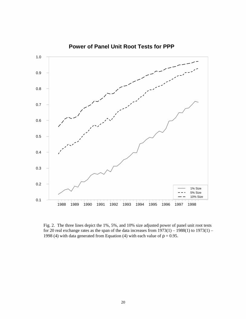
analyze the power of our tests as the span of the data increases. The results are illustrated in Figure 2 for

panels of 20 real exchange rates generated from Equation (4) with the intercept µ = 0 and each value of ρ

= .95. While, as expected, the power of the tests increases with the span of the data, the rise in power is

much too smooth to explain the cycles in the strength of the rejections.

The strengthening of the evidence, moreover, is strongly related to the value of the real exchange

rate at the end of the sample. Figure 3 plots the average real exchange rate relative to the United States

dollar and the p-values of the unit root tests. When the dollar appreciates, the evidence of PPP

4 The critical values decrease (in absolute value) as the span of the data increases, but not exactly monotonically, because they also depend on the serial and contemporaneous correlation in the data. Since this is more pronounced at the 1% level, we suspect that it is also caused by sampling variability, even with 20,000 replications.

7

strengthens and, when it depreciates, the evidence weakens. This is also a puzzling result. It is difficult

to see why evidence of PPP should be stronger when the dollar appreciates. Moreover, when the dollar

appreciates, other currencies depreciate. Any explanation for why the evidence of PPP increases when

the dollar appreciates would also have to explain why the same evidence increases when the mark (for

example) depreciates. These results raise the possibility that the strong rejections of unit roots in real

exchange rates with the dollar as numeraire starting in 1997 may, in part, be an artifact of the appreciation

of the dollar rather than compelling evidence of PPP.

The visual evidence can be supported statistically. Regressing the p-values from the 44 spans of

the data on a constant, trend, trend-squared, and the real exchange rate, we obtain:

p-value = 1.45 - 0.012 t + 0.00017 t2 - 0.53 q , (5)

(5.29) (-4.87) (3.02) (-4.35)

where q is the average dollar real exchange rate and t-statistics are in parentheses. When the dollar

appreciates (q rises), the p-value of the unit root test strengthens (falls). The p-values also strengthen with

the length of the sample, but at a decreasing rate.

The regression results provide additional support for the hypothesis that the increasing evidence

of PPP as the sample length increases is not solely caused by lower critical values. The same results are

found when the (absolute value of) the t-statistic, rather than the p-value, is the dependent variable,

t-statistic = 0.51 + 0.014 t + 3.17 q . (6)

(0.42) (4.59) (5.64)

The t-statistics are both positive and significantly different from zero. They increase with the span of the

data and when the dollar appreciates at the end of the sample. If the strengthening of the evidence was

solely caused by adjusting the critical values as the sample length increases, the t-statistics would be

unrelated to the time trend. 5

3. Data Generating Processes

We have documented that the evidence of PPP from panel unit root tests with industrialized

countries in the post-1973 floating exchange rate period increases with the length of the sample beyond

what would be expected from adjusting the critical values and increases when the dollar appreciates at the

end of the sample. We find both results surprising, and call them (collectively) the “panel purchasing

power parity puzzle.” We attempt to explain the puzzle by using simulation methods. Using a variety of

data generating processes, we artificially generate panels of "real exchange rates" with 20 "countries" and

104 observations (the dimensions of the actual sample). The artificial data is constructed to replicate the

pattern of contemporaneous correlation found in the actual data. We then conduct panel unit root tests on

8

the artificial data, starting with the first 61 observations (corresponding to the initial actual sample), and

adding observations one at a time until all 104 observations are used. Finally, we compare the "evidence"

of PPP found in the actual and simulated data over the 44 sample lengths.

We examine unit root and stationary autoregressive processes, mixed autoregressive processes,

threshold autoregressive processes, and PPP restricted structural change processes. The first metric that

we use is to minimize the root mean squared error (RMSE) between the series of t-statistics generated by

the simulated data, averaged over 1000 draws, and the t-statistics generated by the actual data.6 We

examine whether the vector of t-statistics generated by the simulated data is consistent with the

strengthening and cycles in the evidence of PPP found in the t-statistics from the actual data. Our second

metric is to estimate Equation (6) for each of the 1000 draws and calculate the number of times that the t-

statistics on the time trend and real exchange rate are as large (or larger) than those found in the actual

data. Finally, we develop techniques to compare the fit among the specifications.

3.1 Unit root and stationary autoregressive processes

Consider the AR(1) specification for the real exchange rate in Equation (4). If ρ = 1, the real

exchange rate has a unit root and PPP does not hold. If ρ < 1, the real exchange rate is mean reverting

and PPP does hold. The results of our experiment when ρ = 1 are shown in Figure 4.7 As above, the

negative of the t-statistic on α in Equation (3) is on the vertical axis. This is clearly a terrible

specification. The t-statistics from the generated data are far smaller (in absolute value) than the t-

statistics from the actual data for all sample lengths.

What value of ρ maximizes the congruence between the actual and the simulated data? Based on

trial-and-error experimentation, we found that a value of ρ = .972 minimized the RMSE between the

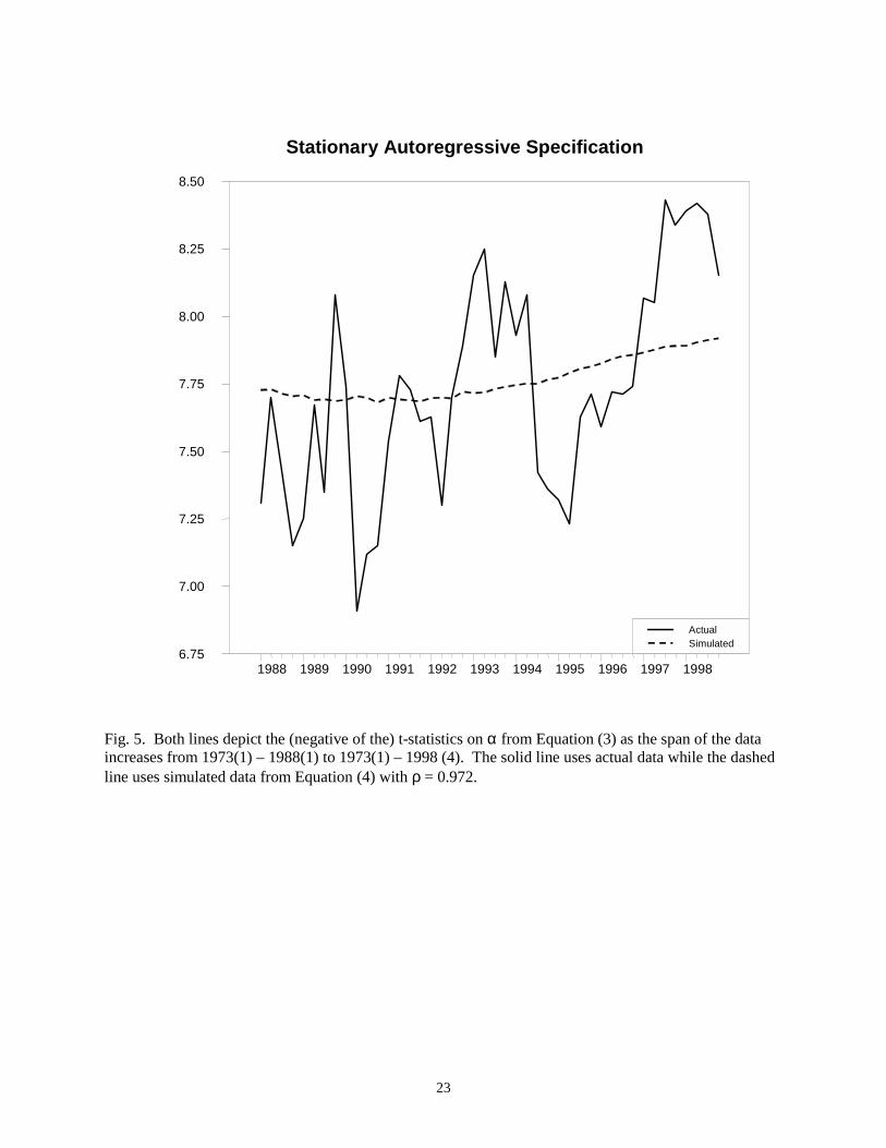
actual and simulated t-statistics.8 As depicted in Figure 5, however, even the best AR(1) specification

fails to match two characteristics of the actual data. First, the t-statistics from the simulated data increase

(in absolute value) only slightly as the span of the data lengthens, while those from the actual data

increase much more. Second, the cyclical pattern of the t-statistics, found in the actual data, is not found

at all in the generated data.

The value of ρ = .972 seems "too high" in the following sense. The half-lives of PPP deviations,

the expected number of years for a disturbance to the real exchange rate to decay by 50 percent, are

generally calculated to be about 2.5 years with panel methods for post-1973 real exchange rates with the

5 The trend-squared term is not significant when the t-statistic is the dependent variable. 6 There is an exact correspondence between comparing t-statistics and p-values, and the former is much less computationally burdensome. 7 Because the intercept µ = 0 under the unit root null, the data is generated without an intercept in order to avoid biasing the estimates. The estimated regression, however, allows for country-specific intercepts as in Equation (3). 8 The RMSE’s for all specifications are reported in Column 1 of Table 1.

9

U.S. dollar as the numeraire currency. With ρ = .972, the half-life would be much larger, about 6.1 years.

It is well known, however, that OLS estimates of autoregressive models are biased downward, with the

bias worsening the closer the autoregressive root is to unity. The same issue arises with SUR estimates of

panel autoregressive models. For the full span of the data, the average value (across the 1000

replications) of α in Equation (3) is -.064. This implies a value of ρ = .936 when the generated value of ρ

= .972, producing a half-life of 2.26 years.9

Because the series of t-statistics for the simulated data are averaged over 1000 draws, they

smooth out fluctuations in the individual series. We computed, but do not report, the 95% confidence

interval for the t-statistics around the sampling mean. They exhibit considerable sampling variation,

certainly enough to encompass the cyclical behavior observed in the actual t-statistics. In addition, the

individual series of t-statistics for the simulated data display substantial variation. This raises the

possibility that the observed pattern of t-statistics for the actual data, rather than being a stylized fact to be

explained, is just noise.

In order to investigate the possibility that the observed pattern of t-statistics is simply noise, we

estimate Equation (6) for each of the 1000 draws using generated data with ρ = .972 and tabulate how

many times the t-statistics on the time trend and real exchange rate are both greater than the t-statistics on

those coefficients reported in Equation (6) for the actual data. The rejection frequency is .025, meaning

that, if the data was generated by an AR(1) with ρ = .972, equally strong or stronger results than reported

in Equation (6) would be found only 2.5 percent of the time. This shows that the coefficients on the time

trend and real exchange rate found in the actual data are unusual in the set of t-statistics from the

simulated data and, therefore, that the observed pattern of t-statistics is not just noise.

3.2 Mixed unit root/stationary autoregressive processes

Engel (2000) writes the log of the real exchange rate, qt, as the sum of two components, xt and yt,

where xt is the deviation of the law of one price for traded goods and yt is the relative price of non-traded

goods. He assumes that yt follows a simple random walk and xt is stationary and follows an AR(1)

process. Using disaggregated data for the United Kingdom for 1970 - 1995, he generates real exchange

rates from the following model:

ttt yxq += , (7)

,11 ++ =− ttt auyy (8)

,1111 )()( ++++ −+−+−= ttttt ugbvfcdxx ερ (9)

9 This is almost exactly equal to the bias reported in Andrews (1993) for a univariate first-order autoregressive model with 100 observations.

10

where c, f, b, and g are estimated parameters and ut, vt, and εt are i.i.d., N(0,1) random variables. The

estimated value of ρ = .923 and the innovation variance of xt is nearly 100 times as large as the innovation

variance of yt.10

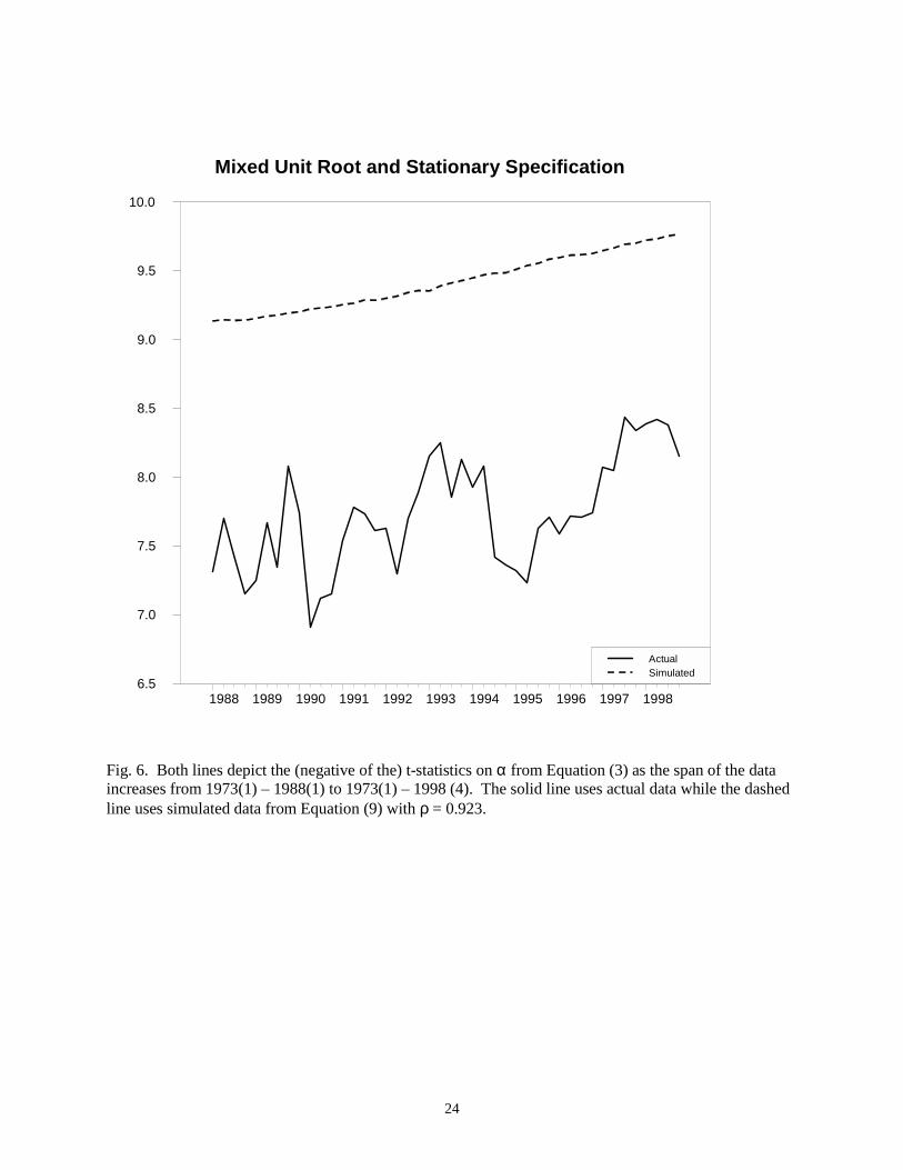
Using Engel's estimated parameter values, we generate panels of "real exchange rates" from

Equations (7) - (9) and conduct the same simulation as described above. The results of the experiment are

shown in Figure 6. Looking only at the simulated t-statistics, this appears to provide very strong

confirmation, in a short-horizon panel setting, of Engel's long-horizon univariate results. Even though the

series, as sums of stationary and unit root processes, all have unit roots by construction, the unit root null

is rejected at the 5% level for each of the 44 sample lengths.

The problem with these results is that they are too strong. The simulated t-statistics are much

larger than the actual t-statistics. Suppose that post-1973 real exchange rates were well described by

Engel's estimated parameter values. In that case, we should have seen strong rejections of the unit root

null for all of the sample lengths, not just the samples extending to 1997 and 1998. As with the stationary

AR(1) model, we use trial-and-error methods and determine that a value of ρ = .970 maximizes the

congruence between the actual and the simulated data. The results of this experiment, depicted in Figure

7 for the average t-statistics and by a rejection frequency of .028 for the vector of t-statistics, are very

similar to the stationary AR (1) specification with ρ = .972.11 This illustrates the concept of near

observational equivalence between unit root and stationary, but highly persistent, processes.12

4. Nonlinear mean reversion

There has been considerable recent interest in the hypothesis of nonlinear adjustment to PPP. We

examine whether two specifications of nonlinear mean reversion, threshold autoregressive processes and

exponential smooth transition autoregressive processes, are better able to account for the pattern of

increasing and cyclical evidence of PPP than the linear specifications discussed above.

4.1 Threshold autoregressive processes

Obstfeld and Taylor (1997) and Taylor (2001) postulate that, because of transactions costs, there

is a band within which the real exchange rate follows a random walk. Outside the band, there is linear

reversion to the edge of the band. Taylor (2001) models this as a symmetric two-regime threshold

autoregression (TAR):

tt cqc ερ +−++ − )( 1 if cqt >−1 ,

10 The parameter estimates and the derivation of the decomposition can be found in Engel (2000). 11 The RMSE for the mixed unit root/stationary autoregressive process is larger than the RMSE for the stationary autoregressive process. We develop methods for testing whether the difference is statistically significant in Section 6.

11

=tq ttq ε+−1 if cqc t −≥≥ −1 , (10)

tt cqc ερ +++− − )( 1 if 1−>− tqc ,

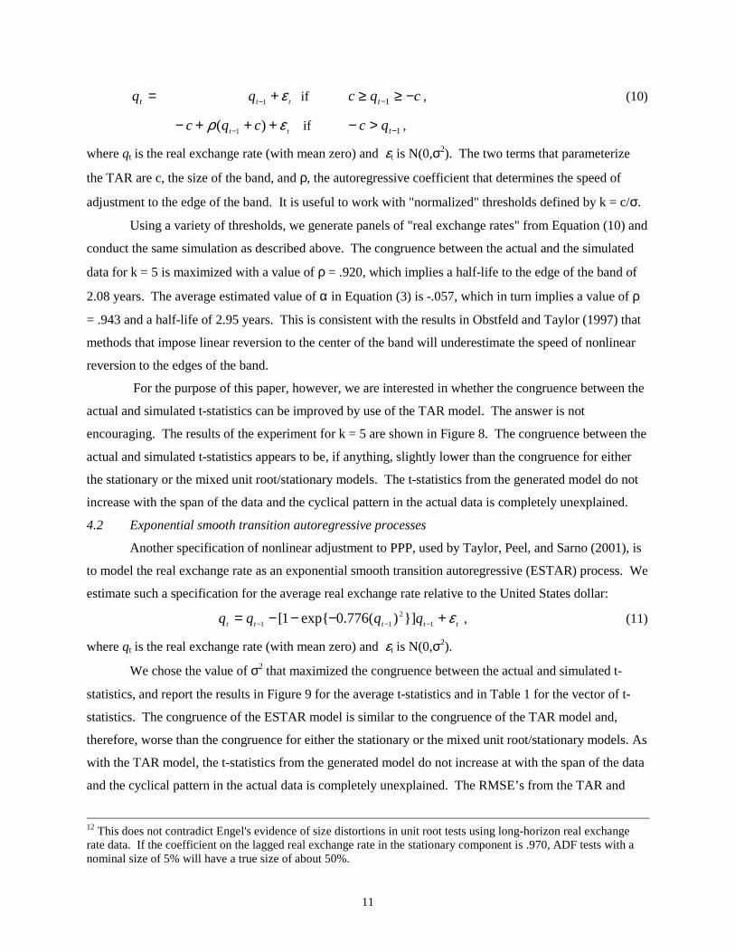
where qt is the real exchange rate (with mean zero) and εt is N(0,σ2). The two terms that parameterize

the TAR are c, the size of the band, and ρ, the autoregressive coefficient that determines the speed of

adjustment to the edge of the band. It is useful to work with "normalized" thresholds defined by k = c/σ.

Using a variety of thresholds, we generate panels of "real exchange rates" from Equation (10) and

conduct the same simulation as described above. The congruence between the actual and the simulated

data for k = 5 is maximized with a value of ρ = .920, which implies a half-life to the edge of the band of

2.08 years. The average estimated value of α in Equation (3) is -.057, which in turn implies a value of ρ

= .943 and a half-life of 2.95 years. This is consistent with the results in Obstfeld and Taylor (1997) that

methods that impose linear reversion to the center of the band will underestimate the speed of nonlinear

reversion to the edges of the band.

For the purpose of this paper, however, we are interested in whether the congruence between the

actual and simulated t-statistics can be improved by use of the TAR model. The answer is not

encouraging. The results of the experiment for k = 5 are shown in Figure 8. The congruence between the

actual and simulated t-statistics appears to be, if anything, slightly lower than the congruence for either

the stationary or the mixed unit root/stationary models. The t-statistics from the generated model do not

increase with the span of the data and the cyclical pattern in the actual data is completely unexplained.

4.2 Exponential smooth transition autoregressive processes

Another specification of nonlinear adjustment to PPP, used by Taylor, Peel, and Sarno (2001), is

to model the real exchange rate as an exponential smooth transition autoregressive (ESTAR) process. We

estimate such a specification for the average real exchange rate relative to the United States dollar:

ttttt qqqq ε+−−−= −−− 12

11 }])(776.0exp{1[ , (11)

where qt is the real exchange rate (with mean zero) and εt is N(0,σ2).

We chose the value of σ2 that maximized the congruence between the actual and simulated t-

statistics, and report the results in Figure 9 for the average t-statistics and in Table 1 for the vector of t-

statistics. The congruence of the ESTAR model is similar to the congruence of the TAR model and,

therefore, worse than the congruence for either the stationary or the mixed unit root/stationary models. As

with the TAR model, the t-statistics from the generated model do not increase at with the span of the data

and the cyclical pattern in the actual data is completely unexplained. The RMSE’s from the TAR and

12 This does not contradict Engel's evidence of size distortions in unit root tests using long-horizon real exchange rate data. If the coefficient on the lagged real exchange rate in the stationary component is .970, ADF tests with a nominal size of 5% will have a true size of about 50%.

12

ESTAR models are larger, and the rejection frequencies from the TAR (.017) and ESTAR (.021) models

are smaller than those from the stationary and mixed unit root/stationary models.13

5. PPP Restricted Structural Change

Conducting panel unit root tests of PPP in post-1973 real exchange rates as the end of the sample

is extended from 1988 to 1998 produced two results. The evidence of PPP increases with the span of the

data and the strength of the evidence is cyclical. We have presented evidence that none of the standard

data generating processes for real exchange rates: unit root; stationary autoregressive; Engel's mixed unit

root and stationary autoregressive; Obstfeld and Taylor's band threshold autoregressive; or Taylor, Peel,

and Sarno's exponentially threshold autoregressive can successfully explain these results. We proceed to

consider less standard processes that are more idiosyncratic to the post Bretton Woods period.

The motivation for the analysis can be seen in Figure 10, which depicts the (unweighted) average

real exchange rate relative to the United States dollar from 1973 to 1998. While the largest movement of

the real exchange rate is clearly the rise and fall of the dollar from 1980 to 1987, there are also several

sizable post-1987 fluctuations. The figure provides a possible rationale for both the increasing strength

and cycles in the evidence of PPP reported above.

Our first hypothesis involves the strength of the evidence. Panel unit root tests, like other

regressions, can be sensitive to the ends of the sample. Papell and Theodoridis (1998), for example, show

that if the sample ends at the peak of the dollar's appreciation, these tests provide absolutely no evidence

of PPP. The 1973 - 1988 sample ends just after the dollar fell. We conjecture that, as the span of the data

extends to include more post -1987 observations, the evidence of PPP will strengthen.

Our second hypothesis involves the cycles in the evidence. The mean value of the dollar for the

full 1973 - 1998 period is considerably higher than the mean value for 1988 - 1998, reflecting the large

appreciation in 1980 - 1985. In fact, every appreciation of the dollar since 1988 represents a movement

towards the full sample mean. This can potentially explain the finding, reported above, that the evidence

of PPP is stronger when the dollar appreciates. Each appreciation of the dollar since 1988 places the end

of the sample closer to the full sample mean.

We investigate these hypotheses by generating panels of "real exchange rates" that mimic the rise

and fall of the dollar and are consistent with PPP. Consider the following process:

tttttt DTDTDTqq εγγγρµ +++++= − 321 3211 . (12)

13 Taylor, Peel, and Sarno (2001) use monthly data and report smaller (in absolute value) coefficients than we find. We experimented with several of their specifications, and the results were unchanged. We also experimented with altering the value of the (exponentially) autoregressive coefficient, but the congruence was maximized by making the coefficient so small as to eliminate the nonlinearity. Since ADF tests have low power if the true process is nonlinear, this did not provide a fair test of the fit of the ESTAR model.

13

The breaks occur at times TB1, TB2, and TB3, and the dummy variables DTi t = (t - TBi) if t > TBi , 0

otherwise, i = 1,…, 3. There are three changes in the slope: the first to account for the start of the dollar's

rise, the second to account for the switch from rise to fall, and the third to account for the end of the fall.

Purchasing power parity is imposed by the restrictions,

0321 =++ γγγ , (13)

which imposes a constant mean following the third break, and

0)23()13( 21 =−+− TBTBTBTB γγ , (14)

which restricts the mean following the third break to equal the mean prior to the first break. For

consistency with PPP, there is a constant mean (no time trend) prior to the first break.

In Papell (2002), we develop methods that test the null hypothesis of a unit root without structural

change against the alternative hypothesis of level stationarity with "PPP restricted structural change." We

find that, for the (mostly European) countries that adhere to the typical pattern of the dollars rise and fall,

these methods provide much stronger evidence than conventional panel unit root tests that do not account

for structural change. Our objective in this paper is different. We want to see whether data generated to

be consistent with PPP restricted structural change can improve the congruence, using conventional tests,

between the actual and simulated t-statistics.

Although the choice of three breaks in the slope was dictated by our desire to model the rise and

fall of the dollar, it can be supported statistically. Bai (1999) develops likelihood ratio tests for multiple

structural changes that allow for trending data and lagged dependent variables. Using his tests on the

average (unweighted) real exchange rate, we find breaks in 1979(3), 1984(3), and 1987(1). The zero, one,

and two break nulls are rejected against the three break alternative at the 5 percent level, and the three

break null is not rejected against the four break alternative at the 10 percent level. We then ran the

regression (12), subject to the restrictions (13) and (14), and found that γ1 = 0.006, γ2 = -0.019, and γ3 =

0.013.

We proceed to generate panels of "real exchange rates" from Equation (12) and conduct the same

simulation as described above. The results of the experiment are shown in Figure 11 for a value of ρ =

.887, which maximized the congruence between the actual and simulated t- statistics. The RMSE is lower

than the RMSE's for the stationary AR, mixed unit root/stationary, TAR, and ESTAR models, and the t-

statistics rise as the sample length increases. The PPP restricted structural change model can thus account

for one of the stylized facts, the strengthening of the t-statistics as the span of the data lengthens, that

cannot be explained by the other models. It cannot, however, account for the other stylized fact, the

cyclical evidence of PPP observed in the actual data. The rejection frequency is .046. While this is larger

than the rejection frequencies for the other specifications, it provides confirmation that the PPP restricted

structural change model cannot account for both stylized facts.

14

6. Statistical comparison among specifications

We have made a number of claims based on visual evidence and informal comparison of

RMSE's. We find that the pattern of evidence is best explained by a specification with PPP restricted

structural change, one cannot choose between stationary autoregressive and Engel's mixed unit

root/stationary autoregressive processes, and one cannot choose between TAR and ESTAR specifications.

We proceed to develop statistical techniques to compare the specifications.

Consider two specifications of data generating processes. We want to test the null hypothesis that

the fit of the two processes are the same against the alternative hypothesis that the fit of the process with

the smaller (larger) RMSE is better (worse) than the fit of the process with the larger (smaller) RMSE.

Since we are not aware of any appropriate statistical tests, we use simulation methods to develop tests that

are specific to our particular specifications and data.

We simulate under the null by calculating 750 RMSE's for each DGP that differ only by the

choice of the seed value for the random number generator.14 We then compare the median RMSE for

each process against the ordered set of RMSE’s from each of the other four processes. If the median

RMSE for a process lies above the upper 97.5 percent fractal or below the lower 2.5 percent fractal for a

different process, we reject the null hypothesis that the fit of the two processes is the same at the 5 percent

level. We use the median RMSE to ensure against the possibility of rejecting the null that the fit of two

specifications are the same because we have chosen an RMSE that is unusual in its own distribution.

The median RMSE’s, critical values and test results are reported in Table 1. The order of the

median RMSE’s (smallest to largest) is structural change, stationary autoregressive, mixed unit

root/stationary autoregressive, ESTAR and TAR. For each pair of RMSE’s, we conduct two tests. First,

we see if the smaller median RMSE is below the 2.5 percent fractal of the process for the larger median

RMSE. If so, we reject the null hypothesis that the fit of the two processes are the same in favor of the

alternative hypothesis that the fit of the process with the smaller median RMSE is better than the fit of the

process with the larger RMSE at the 5 percent level. Second, we see if the larger median RMSE is above

the 97.5 percent fractal of the process for the smaller median RMSE. If so, we reject the null hypothesis

that the fit of the two processes are the same in favor of the alternative hypothesis that the fit of the

process with the larger median RMSE is worse than the fit of the process with the smaller RMSE at the 5

percent level. The two tests do not necessarily coincide.

We discuss several examples in detail. First, not only is the median RMSE of the structural

change specification lower than the RMSE’s of the other specifications, but the upper 97.5 fractal of the

15

structural change specification is lower than the bottom 2.5 percent fractal of any of the other

specifications, so the null hypothesis that the fit of the structural change specification is the same as any

of the others’ is overwhelmingly rejected. Second, while the median RMSE of the stationary

autoregressive specification (.367) is smaller than the median RMSE of the mixed unit root/stationary

autoregressive specification (.376), the lower 2.5 percent fractal for the mixed unit root/stationary

autoregressive specification is .362 and the upper 2.5 percent fractal for the stationary autoregressive

specification is .384, so the null that the fit is the same cannot be rejected at the 5 percent level in either

case. The p-values are .27 when the stationary autoregressive specification is the null and .18 when the

mixed unit root/stationary autoregressive specification is the null. Third, while the median RMSE of the

ESTAR specification (.401) is smaller than the median RMSE of the TAR specification (.404), the

difference is clearly not significant. The p-values are .77 when either specification is the null.

There are four cases where the statistical evidence is sharper than the visual evidence – all

involving comparisons between the stationary autoregressive and mixed unit root/stationary

autoregressive specifications and the TAR and ESTAR specifications. For example, the median RMSE of

the stationary autoregressive specification (.367) is smaller than the median RMSE of the ESTAR

specification (.401). The lower 2.5 percent fractal for the ESTAR specification is .387 and the upper 2.5

percent fractal for the stationary autoregressive specification is .384, so the null that the fit is the same can

be rejected at the 5 percent level in both cases. The p-value is .00 with either specification as the null.

Similar results are found for the other three cases.

The overall results of the statistical test confirm the visual evidence. First, the models without

structural change can easily be rejected in favor of the model with structural change. Second, there is no

evidence to choose between the stationary autoregressive and mixed unit root/stationary autoregressive

models. Third, there is no evidence to choose between the TAR and the ESTAR models. Finally, the

TAR and ESTAR models can be rejected in favor of the stationary autoregressive and mixed unit

root/stationary autoregressive models. This is the only case where the statistical evidence is sharper than

the visual evidence.

7. Conclusions

The post Bretton-Woods period of flexible exchange rates, 1973 to 1998, provides an almost ideal

setting for panel unit root tests of purchasing power parity for industrialized countries.15 While the span

14 Each calculation of an RMSE takes between 45 and 60 minutes on a fairly fast desktop computer, so performing numerous simulations becomes computationally burdensome. With 500 or more replications, the 2.5% and 97.5% fractals did not change to the third decimal point. 15 Two caveats (at least) are in order. First, exchange rate arrangements, most notably the European Monetary System, impart a degree of fixing to the intra-European rates. Second, although nominal exchange rates are available either end-of-sample or period-averaged, the CPI data is only period averaged. Taylor (2001) argues that,

16

of the data is too short for univariate tests to have good power, it is long enough for panel methods. It is

also a data set with a clear endpoint. With the advent of the euro in 1999, the cross rates for 11 of the 20

countries became irrevocably fixed. Whatever we find or don't find, we cannot learn more simply by

extending the data as it becomes available.

The purpose of this paper is to determine what can be learned about real exchange rates with the

United States dollar as the numeraire currency during this period by using panel unit root tests for PPP.

We proceed in two stages. First, using econometric techniques, we document the evidence of PPP as the

span of the data is increased from 1973-1988 to 1973-1998. Second, using simulation methods, we

investigate what data generating processes are consistent with the econometric evidence.

Our econometric results are twofold. First, while the evidence of PPP, measured by the p-values

of the panel unit root tests, increases as the span of the data lengthens, the strengthening is not solely

caused by the increasing length of the sample. Second, the evidence of PPP increases when the dollar

appreciates at the end of the sample. We call these results the “panel purchasing power parity puzzle.”

We proceed to use simulation methods to evaluate these econometric results. Using a variety of

data generating processes, we artificially generate panels of "real exchange rates" that match the

dimensions of the actual sample, conduct panel unit root tests on the artificial data, and compare the

"evidence" of PPP found in the actual and simulated data. While we use a formal metric to evaluate the

processes, we focus here on whether they can replicate two characteristics of the actual data: the

strengthening and cycles in the evidence of PPP as the span of the data increases.

The most popular specification for real exchange rates is an autoregressive process, either

stationary or unit root. We find that, while the stationary specification is clearly preferable to the unit root

specification, it cannot account for either the strengthening or the cycles in the evidence. We then

consider three alternatives, Engel's (2000) mixture of a stationary and a unit root process, Taylor's (2001)

threshold autoregressive process, and Taylor, Peel, and Sarno's (2001) exponential smooth transition

autoregressive process. None of these can account for either the strengthening or the cycles. Finally, we

study a class of "PPP restricted structural change" processes that allow for changes in the slope of the data

generating process, but restrict the pre and post-break means to their PPP level. These results are more

promising. We can account for the strengthening, but not the cycles, of the evidence over time.

especially combined with nonlinear adjustment, time averaging can cause a large downward bias in the speed of adjustment to PPP.

17

References

Abuaf, Niso, and Philippe Jorion (1990). “Purchasing Power Parity in the Long Run.” Journal of Finance 45, 157-174. Andrews, Donald (1993). “Exactly Median Unbiased Estimation of First Order Autoregressive/Unit Root Models.” Econometrica 61, 139-165. Bai, Jushan (1999). “Likelihood Ratio Tests for Multiple Structural Changes.” Journal of Econometrics 91, 299-323. Bowman, David (1999). “Efficient Tests for Autoregressive Unit Roots in Panel Data.” manuscript, Federal Reserve Board. Diebold, Francis, and Robert Mariano (1995). “Comparing Predictive Accuracy." Journal of Business and Economic Statistics 13, 253-265. Engel, Charles (2000). “Long-Run PPP May Not Hold After All.” Journal of International Economics 51, 243-273. Engel, Charles, and James Hamilton (1990). “Long Swings in the Dollar: Are They in the Data and Do Markets Know It?” American Economic Review 80, 689-713. Frankel, Jeffrey, and Andrew Rose (1996). “A Panel Project on Purchasing Power Parity: Mean Reversion Within and Between Countries.” Journal of International Economics 40, 209-224. Hall, Alistair (1994). “Testing for a Unit Root in Time Series with Pretest Data Based Model Selection.” Journal of Business and Economic Statistics 12, 461-470. Higgins, Matthew, and Egon Zakrajsek (1999). "Purchasing Power Parity: Three Stakes Through the Heart of the Unit Root Null." manuscript, Federal Reserve Bank of New York. Im, Kyung So, Hashem Pesaran, and Yongcheol Shin (2003). “Testing for Unit Roots in Heterogeneous Panels.” Journal of Econometrics 115, 53-74. Jorion, Philippe, and Richard Sweeney (1996). “Mean Reversion in Real Exchange Rates: Evidence and Implications for Forecasting.” Journal of International Money and Finance 15, 535-550. Levin, Andrew, Chien-Fu Lin, and James Chu (2002). “Unit Root Tests in Panel Data: Asymptotic and Finite-Sample Properties.” Journal of Econometrics 108, 1-24. Lopez, Claude, and David Papell (2003). “"Convergence to Purchasing Power Parity at the Commencement of the Euro." manuscript, University of Houston. Maddala, G.S., and Shaowen Wu (1999). “A Comparative Study of Unit Root Tests with Panel Data and a New Simple Test.” Oxford Bulletin of Economics and Statistics 61, 631-652. Obstfeld, Maurice, and Alan Taylor (1997). “Nonlinear Aspects of Goods-Market Arbitrage and Adjustment: Heckscher’s Commodity Points Revisited.” Journal of the Japanese and International Economies 441-479.

18

O’Connell, Paul (1998). “The Overvaluation of Purchasing Power Parity.” Journal of International Economics 44, 1-19. Oh, Keun-Yeob (1996). “Purchasing Power Parity and Unit Root Tests Using Panel Data.” Journal of International Money and Finance 15, 405-418. Papell, David (1997). “Searching for Stationarity: Purchasing Power Parity Under the Current Float.” Journal of International Economics 43, 313-332. Papell, David (2002). “The Great Appreciation, the Great Depreciation, and the Purchasing Power Parity Hypothesis.” Journal of International Economics 57, 51-82. Papell, David, and Hristos Theodoridis (1998). “Increasing Evidence of Purchasing Power Parity Over the Current Float.” Journal of International Money and Finance 17, 41-50. Papell, David, and Hristos Theodoridis (2001). “The Choice of Numeraire Currency in Panel Tests of Purchasing Power Parity.” Journal of Money, Credit and Banking 33, 790-803. Taylor, Alan (2001). "Potential Pitfalls for the Purchasing-Power-Parity Puzzle? Sampling and Specification Biases in Mean-Reversion Tests of the Law of One Price." Econometrica 69, 473-498. Taylor, Mark, David Peel, and Lucio Sarno (2001). "Nonlinear Mean Reversion in Real Exchange Rates: Toward a Solution to the Purchasing Power Parity Puzzles." International Economic Review 42, 1015-1042. Wu, Jyh-Lin, and Shaowen Wu (2001). “Is Purchasing Power Parity Overvalued?” Journal of Money, Credit and Banking 33, 804-812. Wu, Yangru (1996). “Are Real Exchange Rates Nonstationary? Evidence from a Panel-Data Test.” Journal of Money, Credit and Banking 28, 54-63.

19

Fig. 1. The solid line plots the (negative of the) t-statistics on α from Equation (3) as the span of the data increases from 1973(1) – 1988(1) to 1973(1) – 1998 (4) while the dashed lines are the 1%, 5%, and 10% critical values of the panel unit root tests.

Results of Panel Unit Root Tests for PPP

1988 1989 1990 1991 1992 1993 1994 1995 1996 1997 1998

6.8

7.2

7.6

8.0

8.4

8.8

9.2

9.6

10.0

t-statistics 1% Crit Values 5% Crit Values 10% Crit Values

20

Fig. 2. The three lines depict the 1%, 5%, and 10% size adjusted power of panel unit root tests for 20 real exchange rates as the span of the data increases from 1973(1) – 1988(1) to 1973(1) – 1998 (4) with data generated from Equation (4) with each value of ρ = 0.95.

Power of Panel Unit Root Tests for PPP

1988 1989 1990 1991 1992 1993 1994 1995 1996 1997 1998

0.1

0.2

0.3

0.4

0.5

0.6

0.7

0.8

0.9

1.0

1% Size5% Size10% Size

21

Fig. 3. The solid line depicts the average real exchange rate relative to the United States dollar and the dashed line represents the p-values of the panel unit root tests in Equation (3) as the span of the data increases from 1973(1) – 1988(1) to 1973(1) – 1998 (4).

Real Exchange Rates and P-Values

1988 1989 1990 1991 1992 1993 1994 1995 1996 1997 1998

2.05

2.10

2.15

2.20

2.25

2.30

2.35

0.00

0.05

0.10

0.15

0.20

0.25

0.30

0.35

Real P-Value

22

Unit Root Specification

1988 1989 1990 1991 1992 1993 1994 1995 1996 1997 1998

6.0

6.5

7.0

7.5

8.0

8.5

Actual Simulated

Fig. 4. Both lines depict the (negative of the) t-statistics on α from Equation (3) as the span of the data increases from 1973(1) – 1988(1) to 1973(1) – 1998 (4). The solid line uses actual data while the dashed line uses simulated data from Equation (4) with ρ = 1.

23

Stationary Autoregressive Specification

1988 1989 1990 1991 1992 1993 1994 1995 1996 1997 1998

6.75

7.00

7.25

7.50

7.75

8.00

8.25

8.50

ActualSimulated

Fig. 5. Both lines depict the (negative of the) t-statistics on α from Equation (3) as the span of the data increases from 1973(1) – 1988(1) to 1973(1) – 1998 (4). The solid line uses actual data while the dashed line uses simulated data from Equation (4) with ρ = 0.972.

24

Mixed Unit Root and Stationary Specification

1988 1989 1990 1991 1992 1993 1994 1995 1996 1997 1998

6.5

7.0

7.5

8.0

8.5

9.0

9.5

10.0

Actual Simulated


25

Mixed Unit Root and Stationary Specification

1988 1989 1990 1991 1992 1993 1994 1995 1996 1997 1998

6.75

7.00

7.25

7.50

7.75

8.00

8.25

8.50

Actual Simulated


26

Threshold Autoregressive Specification

1988 1989 1990 1991 1992 1993 1994 1995 1996 1997 1998

6.75

7.00

7.25

7.50

7.75

8.00

8.25

8.50

Actual Simulated


27

Exponentially Smooth Threshold Autoregression

1988 1989 1990 1991 1992 1993 1994 1995 1996 1997 1998

6.75

7.00

7.25

7.50

7.75

8.00

8.25

8.50

Actual Simulated

Fig. 9. Both lines depict the (negative of the) t-statistics on α from Equation (3) as the span of the data increases from 1973(1) – 1988(1) to 1973(1) – 1998 (4). The solid line uses actual data while the dashed line uses simulated data from Equation (11).

28

Average Dollar Real Exchange Rate 1973-1998

Figure 101973 1976 1979 1982 1985 1988 1991 1994 1997

2.04

2.16

2.28

2.40

2.52

2.64 Exchange Rate Mean 1973-1998 Mean 1988-1998

Fig. 10. The solid line depicts the average real exchange rate relative to the United States dollar. The top dashed line (long dashes) is the 1973 – 1998 mean and the bottom dashed line (short dashes) is the 1988 – 1998 mean.

29

PPP Restricted Structural Change

1988 1989 1990 1991 1992 1993 1994 1995 1996 1997 1998

6.75

7.00

7.25

7.50

7.75

8.00

8.25

8.50

Actual Simulated


30

Table 1 Statistical Comparison among the Specifications

RMSE

(1)

Structural Change

(2)

Stationary

(3)

Unit Root/ Stationary

(4)

ESTAR

(5)

TAR

(6) Structural Change

.32382 - .00 .00 .00 .00

Stationary Autoregressive

.36669 .00 - .18 .00 .00

Unit Root/Stationary Autoregressive

.37568 .00 .27 - .00 .00

ESTAR

.40092 .00 .00 .01 - .77

TAR

.40383 .00 .00 .00 .77 -

Note: The first column of the table reports the median RMSE (out of 750 replications) for the five DGP’s. The other columns report p-values from a test of the null hypothesis that the median RMSE for each DGP could have been generated from the distributions from each of the other four DGP’s. The critical values under the null are taken from the specifications listed above the columns. For example, .27 is the p-value of the test that the median RMSE from the mixed unit root/stationary autoregressive specification (.376) could have been generated by the stationary autoregressive specification and .18 is the p-value of the test that the median RMSE from the stationary autoregressive specification (.367) could have been generated by the mixed unit root/stationary autoregressive specification. The 2.5 percent and 97.5 percent fractals of the RMSE’s under the null, which represent 5 percent critical values, are (.319, .329) for the structural change, (.352, .383) for the stationary autoregressive, (.362, .395) for the mixed unit root/stationary autoregressive, (.387, .419) for the ESTAR, and (.386, .422) for the TAR specifications.

the panel purchasing power parity puzzledpapell/puzzle.pdfwe call these findings the “panel...

Documents