the martian landscape
TRANSCRIPT
8/8/2019 The Martian Landscape
http://slidepdf.com/reader/full/the-martian-landscape 1/160
8/8/2019 The Martian Landscape
http://slidepdf.com/reader/full/the-martian-landscape 2/160
The MartianLandscape
National Aeronautics and Space Administration
NASA SP-425
By the Viking Lander Imaging Team
Scientific and Technical Information Office
NATIONAL AERONAUTICS AND SPACE ADMINISTRATION
Washington, D.C. 1978
Library of Congress Catalog No. 78-606041
For sale by the Superintendent of Documents,
U.S. Government Printing Office, Washington, D.C. 20402
Stock No. 033-000-00716 / Catalog No. NAS 1.21:425
8/8/2019 The Martian Landscape
http://slidepdf.com/reader/full/the-martian-landscape 3/160
NASA SP-425 — The Martian Landscape 3
Foreword
Not long ago the idea of taking pictures of Mars from its surface was an idea located intermediately
between far out and preposterous. It changed from a dream to a concept about ten years ago with the
advent of the Viking Program. As so often happens in the exploration of space, we were able to push
back the boundaries of the practicable. In retrospect, with success under our belts, it even sounds simple:
put cameras on spacecraft, land them on Mars, take pictures, send them back to Earth. Were it so!
In this book Tim Mutch, leader of the Viking Lander Imaging Team, takes you on a journey spanning
a decade. Suffer with him as he copes with innumerable meetings, arguments, alternate designs,
budget problems, incipient failures, and, at times, sheer exhaustion. Enjoy with him amazement at how
teamwork and dedication can manage the impossible. Share in wonderment at technical intricacy, the
occasional euphoria of success along the way, and the final exhilaration when magnificent
photographs flow back from the rocky plains of Mars.
The Martian Landscape is a tribute to the hundreds of skillful people who made Viking happen.
Thanks to them, you are there.
April 1978
Noel W. Hinners
Associate Administrator for Space Science
National Aeronautics and Space Administration

8/8/2019 The Martian Landscape
http://slidepdf.com/reader/full/the-martian-landscape 4/160
Contents
An Anectodal Account .......................................................................... 5
The Final Test ................................................................................... 5
The Beginnings ................................................................................. 6
Establishing Camera Characteristics ................................................ 8
Talking Our Way to Mars ............................................................... 13
Deadlines ......................................................................................... 14
Design Changes .............................................................................. 15
Manufacturing Problems ................................................................. 19
Cameras Without Pictures ............................................................... 22
The Preprogrammed Image Sequence ............................................ 27
After The Launch ............................................................................ 29
The Viking 1 Landing ..................................................................... 32
The First Color Picture ................................................................... 33
Uplink and Downlink ..................................................................... 34
The Viking 2 Landing ..................................................................... 35The Extended Mission .................................................................... 38
The Future ....................................................................................... 38
Viking 1 Lander Pictures .................................................................... 39
The First Picture ............................................................................. 40
Surveying the Landscape ................................................................ 41
Desert Drifts .................................................................................... 43
Sculpted Layers ............................................................................... 46
Blocks ............................................................................................. 50
Outcrops .......................................................................................... 57
Landing Scars ................................................................................. 59
Behind the Lander ........................................................................... 65
Viking 2 Lander Pictures .................................................................... 75Another First ................................................................................... 75
Tilt ................................................................................................... 75
A Rocky Plain ................................................................................. 77
Enigmatic Troughs .......................................................................... 87
Looking Backward .......................................................................... 91
Rock Textures ................................................................................. 95
The Distant Horizon ...................................................................... 110
Special Effects .................................................................................... 112
Calibration Pictures ....................................................................... 112
Something From Nothing ............................................................. 113
Searching for Movement ............................................................... 114Digging In ..................................................................................... 117
Secondhand Spacecraft ................................................................. 122
The Changing Atmosphere ........................................................... 123
Beyond Mars ................................................................................. 125
Coloring Mars ............................................................................... 126
A Different Perspective ................................................................ 136
The Third Dimension .................................................................... 139
Panoramic Sketches .......................................................................... 145
A Picture Catalog .............................................................................. 146
The Authors ....................................................................................... 153
NASA SP-425 — The Martian Landscape4
8/8/2019 The Martian Landscape
http://slidepdf.com/reader/full/the-martian-landscape 5/160
The Viking Lander Imaging Investigation:
An Anecdotal Account
Thomas A. Mutch
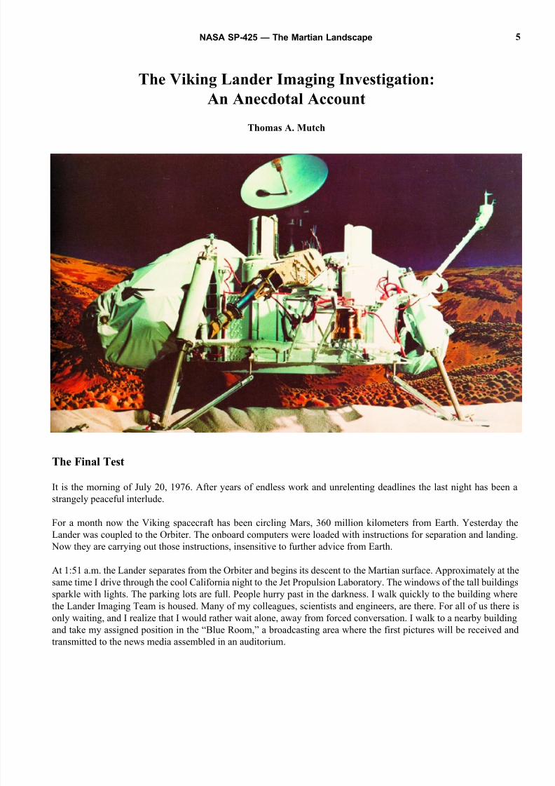
The Final Test
It is the morning of July 20, 1976. After years of endless work and unrelenting deadlines the last night has been a
strangely peaceful interlude.
For a month now the Viking spacecraft has been circling Mars, 360 million kilometers from Earth. Yesterday the
Lander was coupled to the Orbiter. The onboard computers were loaded with instructions for separation and landing.
Now they are carrying out those instructions, insensitive to further advice from Earth.
At 1:51 a.m. the Lander separates from the Orbiter and begins its descent to the Martian surface. Approximately at the
same time I drive through the cool California night to the Jet Propulsion Laboratory. The windows of the tall buildings
sparkle with lights. The parking lots are full. People hurry past in the darkness. I walk quickly to the building where
the Lander Imaging Team is housed. Many of my colleagues, scientists and engineers, are there. For all of us there is
only waiting, and I realize that I would rather wait alone, away from forced conversation. I walk to a nearby building
and take my assigned position in the “Blue Room,” a broadcasting area where the first pictures will be received and
transmitted to the news media assembled in an auditorium.
NASA SP-425 — The Martian Landscape 5
8/8/2019 The Martian Landscape
http://slidepdf.com/reader/full/the-martian-landscape 6/160
5 a.m. The final descent begins. Conversation stops – an overwhelming silence. We listen to the mission controllers as
they call out each event. After years of waiting, hoping, guessing, the end rushes toward us – too fast to reflect, too
fast to understand.
5:05 a.m. “400 000 feet”
5:09 a.m. “74 000 feet”
5:11:43 a.m. “2600 feet”
5:12:07 a.m. “Touchdown. We have touchdown.”
It worked! Amazingly, it worked. Everywhere people are cheering, shaking hands, embracing. I decide not to join
the celebration. It is too soon. Forty minutes more remain before the first picture from the surface of a far planet will
assemble on the television screen.
5:54 a.m. I study the blankness of the television screen, waiting for the narrow strip of light that will signal the first
few lines of the first picture. And it appears. A sliver of electronic magic. Areas of brightness and darkness. The
picture begins to fill the screen. Rocks and sand are visible and – finally, at the far right – one of the spacecraft foot
pads, a symbolic artifact that stamps our accomplishment with the sign of reality.
I wait impatiently for the second picture, a 300° panorama looking out toward the horizon. On Mars the camera carried
out its slow, arcing traverse minutes ago. Now rock-strewn ridges, drifts of sand, distant bluffs slowly pass before me.
All this time I critique, for the audience watching elsewhere, the landscape we are viewing. It is not a task I have been
looking forward to. But now excitement washes over my inhibitions.
Time and time again I repeat, “It’s incredible.” And it truly is. Nothing before or after can compare. It is transparent,
brilliant, boundless. An explorer would understand. We have stood on the surface of Mars.
6:52 a.m. The first two pictures end. The Orbiter, which has been relaying these first images to Earth, drops below
the horizon, and the Lander prepares for its first night on the surface of Mars. On Earth, we plan for the days ahead.
The Beginnings
We live in an age with little patience for history. I was frequently reminded of that in the first few days after our
successful landing on Mars. Continually I was asked, “What are your thoughts as you look at these pictures?” What
were my thoughts? A kaleidoscope of memories eight years of planning, moments of frustration, friendships forged
by common problems, and now everything happening just as we had disbelievingly promised each other it would.
The first few times I was asked about my thoughts I tried to describe those eight years embedded in the first picture.
And that was when I discovered that history was not the subject of the hour. Quickly enough I learned to give the
desired response, a crisp geologic description sprinkled with superlatives, sized to fit a 30 sec spot on tomorrow’s news
program. But I continue to think about the history. If you want to appreciate these pictures fully, you have to travel
with us as the Viking Project is transformed slowly and painfully from an idea to a durable spacecraft, propelled on its
long journey to Mars.
The Viking Mission was first defined by NASA in 1968. Its predecessor, Voyager, never passed beyond the talking
stage. Starting in 1965 and continuing through 1967, tentative plans had been developed for an integrated long term
program of Martian exploration involving, first, flyby and orbiter missions, and then a series of lander missions in
1973, 1975, and 1977. Each of these Voyager Landers was to be launched by a giant Saturn V rocket. Successive
missions were to contain increasingly sophisticated scientific equipment, culminating in a 90 to 450 kg biological
laboratory in the 1977 Voyager spacecraft. Conjured up during the heyday of Apollo when unlimited budgets were
projected far into the future, the ambitious Voyager program was a victim of general economic retrenchment in the late
1960s. In its stead a very small “hard lander” was briefly considered. In one design a protective balsawood shell broke
NASA SP-425 — The Martian Landscape6

8/8/2019 The Martian Landscape
http://slidepdf.com/reader/full/the-martian-landscape 7/160
open on impact, revealing a squat watermelon sized spacecraft. A camera was positioned on an extendible mast. Little
else in the way of scientific equipment was included. It was recognized that the mission lacked both scientific merit
and exploratory excitement. It was replaced by the more ambitious Viking which, ironically, grew to a point where it
incorporated many of the capabilities originally included in Voyager.
Viking included two Orbiter Lander pairs to be placed into orbit about Mars. Following successful orbit insertion the
Landers would be released and directed toward the surface. Slowed first by aerodynamic drag, then by parachute, and
finally by retrorockets, they were designed for a “soft” landing. At 2.5 m sec the jolt would be something like thatencountered when jumping off a 35 cm high stool on Earth. Except for the parachute phase, the entire sequence would
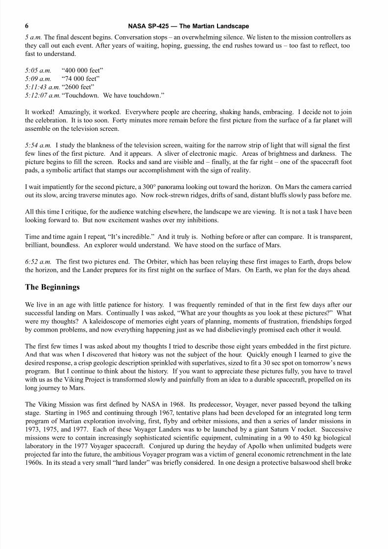
be similar to that employed for Apollo landings on the Moon (Figure 1).
Exactly how is a decision made to fly a particular mission? NASA administrators have at their disposal a number of
planning teams, staffed primarily by engineers and cost analysts. In addition, advisory committees of scientists are
asked to analyze and put in sequence the various mission options. Building on this background, NASA administrators
submit a specific budget with a particular mission called out by name, something termed a “line item.” If the mission
survives subsequent budget trimming by the Office of Management and Budget and Congress, it is elevated to an
“approved” category. Various aerospace companies are invited to submit bids for the construction of the spacecraft,
following the design requirements established by NASA engineers. At the same time an “Announcement of Flight
Opportunity” is widely circulated among universities and research laboratories. Scientists wishing to propose a
scientific experiment of their own choosing, or to participate in an experiment already slated for inclusion – a camera
would be a good example – send in their credentials. A disinterested group of scientists meets to consider all
applications, and then to recommend to NASA those considered best qualified.
It is a supremely democratic arrangement. Everyone can respond to the opportunity. In my own case, for several years
I had been involved peripherally in mapping the Moon, using photographic information from Lunar Orbiter missions
I wanted to become more closely involved with space science, but was advised by a NASA official that there was no
middle ground. Either you were a dilettante or you were an approved mission investigator. It so happened, he added
that the deadline for Viking applications was only several weeks away. Armed with little additional information, I
obtained the necessary forms and started filling them out. Midway through I was tempted to chuck the whole venture
A series of questions seemed aimed specifically at revealing my inadequacies. What was my previous research on
Mars? Zero. List my relevant publications. Pretty meager. List the institutional resources that would support myefforts. None. Against my better judgment I persevered, and filed the completed application.
Several months later, having heard nothing and wishing to end the whole debacle, I called NASA. To my amazement,
my name was recognized, and a man told me that official announcements would be made in a few days. Conservative
and skeptical though I am, I sensed that this reception hinted at good news. Sure enough, my application was approved.
The initial Lander Imaging Planning Team also included Alan Binder, an astronomer then at the IIT Research Institute
Elliott Levinthal, a physicist at Stanford University; Elliot Morris, a geologist with the U.S. Geological Survey; and
Carl Sagan, an astronomer exobiologist at Cornell University. Subsequently, the team was enlarged to include Fred
Huck, a research engineer at NASA Langley Research Center; Sid Liebes, a physicist at Stanford University; Jim
Pollack , a physicist astronomer at NASA Ames Research Center; and Andy Young, an astronomer at Texas A&M
University. We profited enormously from the counsel of Bill Patterson, Brown University, who served as teamengineer, and Glenn Taylor, an engineer administrator who supervised the development of the cameras in behalf of the
Langley Research Center and served as liaison between our team and the rest of the Viking Project.
My first person to person contact with Viking came when Gerry Soffen, Project Scientist, and Tom Young, Science
Integration Manager, journeyed to Providence in the fall of 1968. The stated purpose was to explore a possibility that
I would become leader of the Lander Imaging Planning Science Team. Basically, I suspect they were curious to meet
someone they knew only by name. I recall that we had a pleasant lunch. There was excited talk about all that lay
ahead. But we had no way of anticipating that it was the start of a professional alliance and personal friendship that
would stretch forward, day after day, for eight years.
NASA SP-425 — The Martian Landscape 7
8/8/2019 The Martian Landscape
http://slidepdf.com/reader/full/the-martian-landscape 8/160
All early planning was conducted at the Langley Research Center in Hampton, Virginia. Our first task was to meet
there, all the scientists recently selected some 60 in number and the engineers who had been considering the design of
the mission for almost a year. During the meeting we heard extravagant promises regarding the scientific possibilities
of Viking. It was heady fare.
Figure 1. The sequence of events from launch to landing on Mars.
Establishing Camera Characteristics
Inevitably there is something haphazard about the initial stages of planning a complicated space probe. It is easy to
talk in general terms about the scientific questions to be asked, even to list the general types of instruments to be
employed. But a spacecraft is not made up of generalities. It is composed of millions of parts, each manufactured with
specified characteristics to carry out a particular function.
NASA SP-425 — The Martian Landscape8
8/8/2019 The Martian Landscape
http://slidepdf.com/reader/full/the-martian-landscape 9/160
How is the gap bridged between generality and specificity? In this instance, it is accomplished by the writing of a
document that describes in engineering terms exactly what the scientist-customers wish. This document is then
circulated among private industry. Any company that wishes to compete for the business makes a bid.
Note that the camera is described in “engineering” rather than “scientific” terms. There is an underlying tension
separating the two. Take one of the more obvious camera characteristics, spatial resolution. The scientific goal is to
take pictures of the sharpest clarity, showing the smallest detail. But you can’t very well ask the manufacturer to give
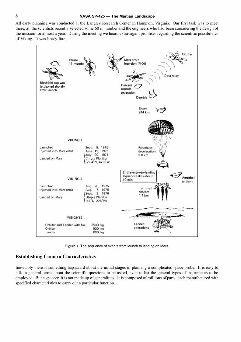
you a “best” picture. Instead we elected to specify that the resolution should be 0.04°. This is sometimes termed thecamera’s instantaneous field of view. The concept is best illustrated by looking at an enlargement of a Viking picture
(Figure 2). With high magnification the image is seen to comprise a regular checkerboard of spots, each with a
particular shade of gray. Each space on the checkerboard approximates a circle which subtends 0.04° as viewed from
the camera position. A single trace of 360° includes 9000 checkerboard squares. A 60° swath in elevation includes
1500. A large panorama, 60° by 360°, comprises the impressively large array of 131/z million checkerboard squares
or pixels (picture elements).
How did we decide to specify a resolution of 0.04°?
The issue was debated at numerous meetings where
we were challenged to demonstrate quantitatively
the increase in scientific return with increase in
resolution. At one point, we were presented with
two pictures of different resolution and asked to
identify the one with the better resolution. The
presenter was trying to develop the argument that,
because we couldn’t differentiate between the two,
it made no difference what the actual camera
resolution was. Predictably the argument collapsed
when everyone correctly identified the two
pictures. In the final analysis, the selected
resolution of 0.04° was an educated guess of the
best that was instrumentally possible.
Over the course of several years, one of our team
members, Fred Huck, already had analyzed
extensively the design tradeoffs between
performance capability and engineering complexity.
He had a thorough familiarity with engineering
practicalities. It was he who sat down with Glenn
Taylor, and, in a matter of a few days, conjured up
the majority of detailed manufacturing specific-
ations. Jumping ahead in our story, it is interesting
to note that after nearly two Earth years of operation
on the surface of Mars the cameras are still perf-
orming according to their original specifications.
Certain camera characteristics were dictated by
spacecraft constraints. Notable among these were
weight, power, and bit rate. The first two are
obvious, but the third deserves some comment.
Cameras generate a great deal of information in a
very short time. This implies some mechanism for
storing all that information. In a conventional
camera the film is that storage device. In a
television camera system the data is generally
NASA SP-425 — The Martian Landscape 9
Figure 2. A part of the first picture taken on the surface of Mars,
and a greatly magnified region within that picture.
Note that the picture comprises a large array of discrete
spots which range in brightness from white to black.
8/8/2019 The Martian Landscape
http://slidepdf.com/reader/full/the-martian-landscape 10/160
stored on magnetic tape. When the Viking mission was conceived, it was known that the entire spacecraft would have
to be sterilized to avoid the possibility of carrying any Earth organisms to Mars. The procedure adopted was heat
sterilization. Just before launch the entire spacecraft would be placed in an oven, and heated to 110°C for
approximately 40 hours. It was feared that neither film nor magnetic recording tape would be stable at that
temperature, and that surface chemicals would volatilize. What was needed was a camera that required no onboard
storage device, but generated data precisely at the rate that it was being transmitted to Earth. Two transmission rates
of 16000 and 250 bits per sec were available, so these same rates were selected for camera operation also.
In the spring of 1970 we met to review the six proposals for camera construction submitted by private industry. Strictly
speaking the decision was not ours. The Martin Marietta Company had already been selected to assemble the entire
Lander. It was their task to identify subcontractors to build the various science instruments. Their choices were subject
to approval by NASA managers at Langley Research Center and Washington Headquarters. Our own team acted as a
science lobby. Working outside the contractual framework, we attempted to persuade those who had to make the
choices. Unfamiliar as we were with the intricacies of business arrangements, we sometimes cynically assumed that our
advice would be ignored. Our concern was unfounded. As the project unfolded, our views were solicited at every point
of decision. Indeed, many times our judgments were requested on subjects where our understanding was more scantily
intuitive than solidly reasoned. Although flattered, I was frequently embarrassed by the willingness of managers to
adopt our suggestions, while tactfully disregarding our general ignorance of spacecraft construction and operation.
As we considered the six camera proposals, one clearly ranked above the others. The technical section was crisply
written. It was obvious that the proposing company, using their own funds, had made detailed preliminary calculations.
The proposed camera design was elegant, avoiding failure-prone mechanically moving parts and gears in favor of
electronic components. There was only one problem. The price tag was much higher than that of the low bidder. Not
only that, some competing companies could point to considerable experience, much of it with NASA endorsement, in
the development of cameras for planetary spacecraft. Although the Viking Project was in its infancy, concerns about
escalating costs had already surfaced. We presented our case with little optimism, and were amazed when the decision
was announced. The cameras would be built by the company we favored, the ITEK Corporation of Lexington, Mass.
The ITEK-built instrument is called a facsimile camera. The name is inherited from a technique in telegraphy whereby
a picture is divided into a grid of small squares. The brightness of each square is converted into an electrical signal.
A sequence of signals sent over the telegraph wire serves as a blueprint for registering the equivalent array of squareson photographic film at the receiving end. In this way, a “facsimile” of the original picture is produced.
In the ITEK design this general concept was refined to produce an instrument with amazing accuracy and versatility. An
essential feature is that the pixels are acquired in relatively slow sequence, thereby meeting the requirement for operation
without tape recorder support. It differs from a conventional camera in that at no time is a complete image recorded in
the focal plane. Instead of film, there is a tiny photosensor fitted with a mask permitting it to view a solid angle of 0.04°
in the object scene. For low-resolution, color, and infrared sensors the view angle is three times larger, 0.12°.
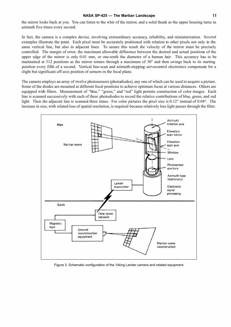
A simplified view of the camera configuration is shown in Figure 3. Light from the scene is reflected from a mirror,
nodding back and forth around a horizontal axis. Focused through a lens system, it is recorded on a photosensor in the
focal plane. Each time the mirror nods, light from successive points along a single apparent vertical line in the object
scene is recorded by the photosensor. When this cycle is completed, the entire upper assembly of the camera movesa small amount around an azimuth rotation axis so that an adjacent vertical line is scanned. As more and more vertical
lines are recorded the picture builds in the azimuthal or “horizontal” dimension, moving from left to right, and, given
enough time, providing a continuous panorama up to 342.5°.
An alternate way of conceiving camera operation is to imagine you could miniaturize yourself and peer through the
small pinhole in the focal plane that is the photosensor aperture. All that you would see would be a flickering light.
Each change in light level would document a transition between a bright and dark region in a vertical line.
In a superficial sense the operation of the camera is remarkably simple. As it goes about its business you can watch
the slotted window in front of the mirror slowly move in a clockwise arc. You can detect a regular sparkle of light as
NASA SP-425 — The Martian Landscape10
8/8/2019 The Martian Landscape
http://slidepdf.com/reader/full/the-martian-landscape 11/160
the mirror looks back at you. You can listen to the whir of the mirror, and a solid thunk as the upper housing turns in
azimuth five times every second.
In fact, the camera is a complex device, involving extraordinary accuracy, reliability, and miniaturization. Several
examples illustrate the point. Each pixel must be accurately positioned with relation to other pixels not only in the
same vertical line, but also in adjacent lines. To assure this result the velocity of the mirror must be precisely
controlled. The margin of error, the maximum allowable difference between the desired and actual positions of the
upper edge of the mirror is only 0.01 mm, or one-tenth the diameter of a human hair. This accuracy has to bemaintained at 512 positions as the mirror rotates through a maximum of 30° and then swings back to its starting
position every fifth of a second. Vertical line-scan and azimuth-stepping servocontrol electronics compensate for a
slight but significant off-axis position of sensors in the focal plane.
The camera employs an array of twelve photosensors (photodiodes), any one of which can be used to acquire a picture
Some of the diodes are mounted at different focal positions to achieve optimum focus at various distances. Others are
equipped with filters. Measurement of “blue,” “green,” and “red” light permits construction of color images. Each
line is scanned successively with each of three photodiodes to record the relative contributions of blue, green, and red
light. Then the adjacent line is scanned three times. For color pictures the pixel size is 0.12° instead of 0.04°. The
increase in size, with related loss of spatial resolution, is required because relatively less light passes through the filter
Figure 3. Schematic configuration of the Viking Lander camera and related equipment.
NASA SP-425 — The Martian Landscape 11
8/8/2019 The Martian Landscape
http://slidepdf.com/reader/full/the-martian-landscape 12/160
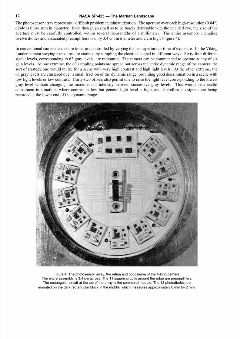
The photosensor array represents a difficult problem in miniaturization. The aperture over each high-resolution (0.04°)
diode is 0.041 mm in diameter. Even though so small as to be barely detectable with the unaided eye, the size of the
aperture must be carefully controlled, within several thousandths of a millimeter. The entire assembly, including
twelve diodes and associated preamplifiers is only 3.4 cm in diameter and 2 cm high (Figure 4).
In conventional cameras exposure times are controlled by varying the lens aperture or time of exposure. In the Viking
Lander camera varying exposures are attained by sampling the electrical signal in different ways. Sixty-four different
signal levels, corresponding to 63 gray levels, are measured. The camera can be commanded to operate at any of sixgain levels. At one extreme, the 63 sampling points are spread out across the entire dynamic range of the camera, the
sort of strategy one would utilize for a scene with very high contrast and high light levels. At the other extreme, the
63 gray levels are clustered over a small fraction of the dynamic range, providing good discrimination in a scene with
low light levels or low contrast. Thirty-two offsets also permit one to raise the light level corresponding to the lowest
gray level without changing the increment of intensity between successive gray levels. This would be a useful
adjustment in situations where contrast is low but general light level is high, and, therefore, no signals are being
recorded at the lower end of the dynamic range.
Figure 4. The photosensor array, the retina and optic nerve of the Viking camera.
The entire assembly is 3.4 cm across. The 11 square circuits around the edge are preamplifiers.
The rectangular circuit at the top of the array is the command module. The 12 photodiodes are
mounted on the dark rectangular block in the middle, which measures approximately 6 mm by 2 mm.
NASA SP-425 — The Martian Landscape12

8/8/2019 The Martian Landscape
http://slidepdf.com/reader/full/the-martian-landscape 13/160
All these operations – diode selection, sampling rates, and video signal
processing – are controlled by complex electronic circuits in the lower
camera assembly. As the camera design evolved, more and more
circuits were crowded on the mounting boards, resulting in an
impressive electronic labyrinth.
Viking Camera Spatial Characteristics
Talking Our Way to Mars
No account of Viking would be complete without mention of the meetings. In a large program, involving many
persons with different backgrounds, interests, and tasks, communication is a major activity. Reams of printed material
are distributed every day. Whenever a decision of some importance was imminent – almost a daily event – a meeting
was convened. There were literally hundreds of committees within Viking. In my case, the more important groups
NASA SP-425 — The Martian Landscape 13
Figure 5. Checking performance of the camera
electronics. The technician uses the headset to
communicate with a second person who obs-
erves the quality of the video signal, displayed
on a television monitor in another room.
General Viking Camera Characteristics
8/8/2019 The Martian Landscape
http://slidepdf.com/reader/full/the-martian-landscape 14/160
were the scientists working on the Lander Imaging Investigation, the engineers designing the camera system, and the
leaders from all science teams comprising the Science Steering Group. During the eight years before launch I must
have attended more than 400 meetings Initially, the opportunity to fly to some distant city was an exotic diversion. But
not for long. The routes to Hampton, Denver, Los Angeles, and Orlando – localities of Viking activity – became as
familiar as the quarter-mile route from my home to my office at Brown University. That peculiar disorientation in both
time and space that results from a long airplane trip became an accepted state of mind. One episode stands out. I recall
shuffling out of an airplane late at night after a few hours of half-sleep, and failing to recognize either where I was or
to what end I was traveling. For several moments I had the Kafkaesque feeling that I had somehow lost my identity,that I had become separated from the real world.
I cannot deny the excitement of participating in this nonstop drama of crisis and decision making. Critics might
question the usefulness of frantic racing around the country, with talk the only obvious product, but every meeting
revealed new problems. Each person was obliged to report what progress he had been making. Cover-ups were
impossible. In retrospect, thinking about all the blunt statements of disagreement and criticism, I am surprised that I
can recall no instance when a participant lost his temper – at least to the point of climbing across the table and slugging
his adversary. Everyone seemed to understand that the high stakes left room for neither social niceties nor aberrations.
On the positive side, helpful advice came from unexpected quarters. Useful exchanges of information prevented
isolated journeys up blind alleys. When no obvious solution to a problem was apparent, we proceeded by vote. The
majority opinion dictated the next step. In one sense, that appears absurd. Certain things are matters of fact. To what
useful end can one vote on the proposition that a camera should cost no more than X dollars, whereas a biology
instrument should cost Y dollars? Or that the average Martian atmospheric pressure is 1 percent of the Earth’s
atmosphere as opposed to 0.5 percent? Viewed in another context, an open meeting in which all participants have
equal vote has served Americans well in many previous situations. Perhaps more than we realize, it is a method of
pooling information with which we have grown up. I like to think that the ultimate success of Viking can be traced
back to those countless meetings at which we chewed on one problem after another – hours of thoughtful criticism and,
sometimes, clamorous sharp-edged debate.
Deadlines
Every Viking activity was framed in time. Weekly reports indicated tasks accomplished, and deadlines projectedthrough the next few months. In conference rooms regularly updated calendars documented the days to launch, as well
as hundreds of intervening events.
This emphasis on time was dictated by the nature of the journey to Mars. Approximately every two years Earth and
Mars draw side by side in their respective orbits, an event known as an opposition. For a period of only a few months
just before opposition, the conditions are favorable for a spacecraft to spiral out from Earth to Mars. For all other times,
the thrust of the rockets is inadequate. For this reason, a so-called launch window can be identified years in advance.
Viking was first planned for a 1973 launch. During January of 1970, when the very existence of the mission was
threatened by funding problems, it was decided to delay the launch two years to 1975, spreading the cost over a longer
period. Our disappointment was short-lived. In fact, the delay was something of a reprieve. In retrospect, it is clear
that the spacecraft could never have been designed and constructed by 1973 without seriously compromising both
capability and reliability.
The ultimate deadline, then, was the August-September launch window in the summer of 1975. The spacecraft had to
leave Earth at that time. No excuses. Another two-year delay until 1977 was unthinkable in terms of increased cost
and administrative complexity.
Development of all instruments was keyed to the 1975 date. Working from that deadline backward, a cascading array
of secondary deadlines was identified. A slip of a few weeks in 1971 could endanger the delivery of the hardware to
the Cape Kennedy launch facility in 1975. Everyone understood the penalty. If the instruments were only half-ready,
they would be flown half-ready-or not at all.
NASA SP-425 — The Martian Landscape14
8/8/2019 The Martian Landscape
http://slidepdf.com/reader/full/the-martian-landscape 15/160
Working within these constraints was less of a burden than one might imagine. Indeed, it was an exhilarating change
from our normal activity – in a university, at least – where the business of one day can be deferred to the next day, or
even the next year. The Viking goals were sharp. There were no compromises, no rationalizations. Every problem
required a timely solution.
Only when you move away from a project like Viking – and are no longer controlled by the calendar – do you realize
the impact of that discipline. It affects you in small ways – always keeping an engagement calendar in your pocket
leaving meetings with just enough time to catch a late plane home and in larger ways – looking forward to a futurewhere events yet to come assume the reality of the present. Now that Viking has passed, I sometimes feel adrift
without those signposts stretching out before me through the years ahead.
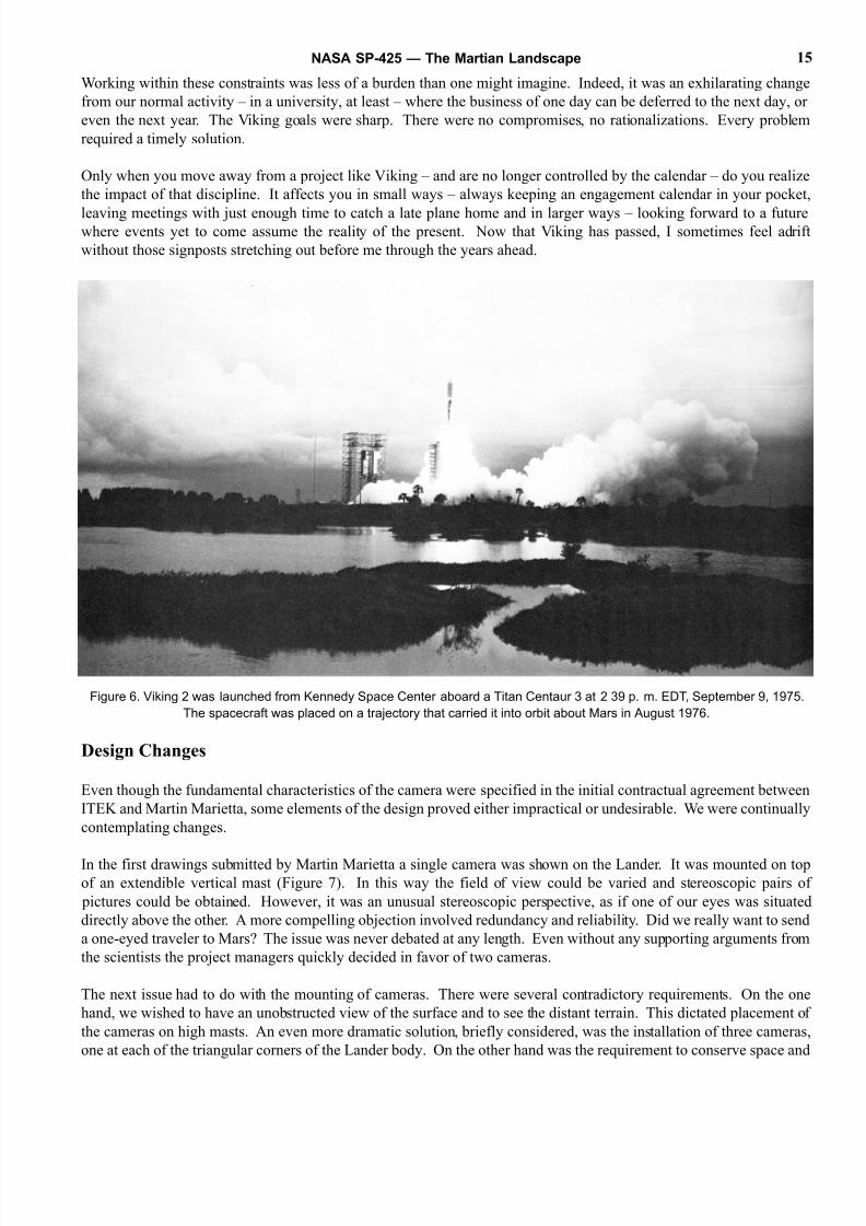
Figure 6. Viking 2 was launched from Kennedy Space Center aboard a Titan Centaur 3 at 2 39 p. m. EDT, September 9, 1975.
The spacecraft was placed on a trajectory that carried it into orbit about Mars in August 1976.
Design Changes
Even though the fundamental characteristics of the camera were specified in the initial contractual agreement between
ITEK and Martin Marietta, some elements of the design proved either impractical or undesirable. We were continually
contemplating changes.
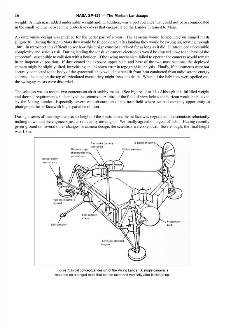
In the first drawings submitted by Martin Marietta a single camera was shown on the Lander. It was mounted on topof an extendible vertical mast (Figure 7). In this way the field of view could be varied and stereoscopic pairs of
pictures could be obtained. However, it was an unusual stereoscopic perspective, as if one of our eyes was situated
directly above the other. A more compelling objection involved redundancy and reliability. Did we really want to send
a one-eyed traveler to Mars? The issue was never debated at any length. Even without any supporting arguments from
the scientists the project managers quickly decided in favor of two cameras.
The next issue had to do with the mounting of cameras. There were several contradictory requirements. On the one
hand, we wished to have an unobstructed view of the surface and to see the distant terrain. This dictated placement of
the cameras on high masts. An even more dramatic solution, briefly considered, was the installation of three cameras
one at each of the triangular corners of the Lander body. On the other hand was the requirement to conserve space and
NASA SP-425 — The Martian Landscape 15
8/8/2019 The Martian Landscape
http://slidepdf.com/reader/full/the-martian-landscape 16/160
weight. A high mast added undesirable weight and, in addition, was a protuberance that could not be accommodated
in the small volume between the protective covers that encapsulated the Lander in transit to Mars.
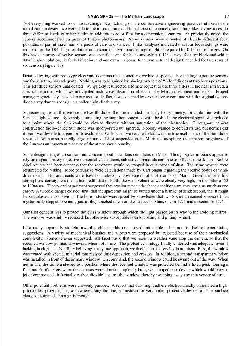
A compromise design was pursued for the better part of a year. The cameras would be mounted on hinged masts
(Figure 8). During the trip to Mars they would be folded down; after landing they would be swung up, rotating through
180°. In retrospect it is difficult to see how this design concept survived for as long as it did. It introduced undesirable
complexity and serious risk. During landing the sensitive camera electronics would be situated close to the base of the
spacecraft, susceptible to collision with a boulder. If the swing mechanism failed to operate the cameras would remainin an inoperative position. If dust coated the exposed upper plate and base of the two mast sections, the deployed
camera might be slightly tilted, introducing an unknown error in topographic analysis. Finally, if the cameras were not
securely connected to the body of the spacecraft, they would not benefit from heat conducted from radioisotope energy
sources. Isolated on the top of articulated masts, they might freeze to death. When all the liabilities were spelled out,
the swing-up masts were discarded.
The solution was to mount two cameras on short stubby masts. (See Figures 9 to 11.) Although this fulfilled weight
and thermal requirements, it dismayed the scientists. A third of the field of view below the horizon would be blocked
by the Viking Lander. Especially severe was obscuration of the near field where we had our only opportunity to
photograph the surface with high spatial resolution.
During a series of meetings the precise height of the masts above the surface was negotiated, the scientists reluctantly
inching down and the engineers just as reluctantly moving up. We finally agreed on a goal of 1.5m. Having recently
given ground on several other changes in camera design, the scientists were skeptical. Sure enough, the final height
was 1.3m.
Figure 7. Initial conceptual design of the Viking Lander. A single camera is
mounted on a hinged mast that can be extended vertically after it swings up.
NASA SP-425 — The Martian Landscape16
8/8/2019 The Martian Landscape
http://slidepdf.com/reader/full/the-martian-landscape 17/160
Not everything worked to our disadvantage. Capitalizing on the conservative engineering practices utilized in the
initial camera design, we were able to incorporate three additional spectral channels, something like having access to
three different levels of infrared film in addition to color film for a conventional camera. As previously noted, the
camera accommodated an array of twelve photosensors. Some sensors were mounted at slightly different foca
positions to permit maximum sharpness at various distances. Initial analyses indicated that four focus settings were
required for the 0.04° high-resolution images and that two focus settings might be required for 0.12° color images. On
this basis an array of twelve sensors was specified: one for black-and-white 0.12° survey, four for black-and-white
0.04° high-resolution, six for 0.12° color, and one extra – a bonus for a symmetrical design that called for two rows ofsix sensors (Figure 11).
Detailed testing with prototype electronics demonstrated something we had suspected. For the large-aperture sensors
one focus setting was adequate. Nothing was to be gained by placing two sets of “color” diodes at two focus positions
This left three sensors unallocated. We quickly resurrected a former request to use three filters in the near infrared, a
spectral region in which we anticipated instructive absorption effects in the Martian sediment and rocks. Project
managers graciously acceded to our request. In fact, it was deemed less expensive to continue with the original twelve-
diode array than to redesign a smaller eight-diode array.
Someone suggested that we use the twelfth diode, the one included primarily for symmetry, for calibration with the
Sun as a light source. By simply eliminating the amplifier associated with the diode, the electrical signal was reduced
to a point where the Sun could be viewed directly without saturation of the electronics. Throughout camera
construction the so-called Sun diode was incorporated but ignored. Nobody wanted to defend its use, but neither did
it seem worthwhile to argue for its exclusion. Only when we reached Mars was the true usefulness of the Sun diode
revealed. With unsuspectedly large amounts of dust suspended in the Martian atmosphere, the apparent brightness of
the Sun was an important measure of the atmospheric opacity.
Some design changes arose from our concern about hazardous conditions on Mars. Though space missions appear to
rely on dispassionately objective numerical calculations, subjective appraisals continue to influence the design. Before
Apollo there had been concerns that the astronauts would be trapped in quicksands of dust. The same worries were
resurrected for Viking. More persuasive were calculations made by Carl Sagan regarding the erosive power of wind-
driven sand. His arguments were based on telescopic observations of dust storms on Mars. Given the very low
atmospheric density, less than a hundredth that of Earth, the wind velocities were clearly very high, on the order of 50to 100m/sec. Theory and experiment suggested that erosion rates under those conditions are very great, as much as one
cm/yr. A twofold danger existed: first, that the spacecraft might be buried under a blanket of sand; second, that it might
be sandblasted into oblivion. The horror stories were spiced by knowledge that two Soviet unmanned spacecraft had
mysteriously stopped operating just as they touched down on the surface of Mars, one in 1971 and a second in 1974.
Our first concern was to protect the glass window through which the light passed on its way to the nodding mirror.
The window was slightly recessed, but otherwise susceptible both to coating and pitting by dust.
Like many apparently straightforward problems, this one proved intractable – but not for lack of entertaining
suggestions. A variety of mechanical brushes and wipers were proposed but rejected because of their mechanical
complexity. Someone even suggested, half facetiously, that we mount a weather vane atop the camera, so that the
recessed window pointed downwind when not in use. The protective strategy finally endorsed was adequate, even iflacking in elegance. Not fully believing in any one approach, we decided that safety lay in numbers. First, the window
was coated with special material that resisted dust deposition and erosion. In addition, a second transparent window
was installed in front of the primary window. On command, the second window could be swung out of the way. When
not in use, the camera slewed to a position where the recessed window was protected behind a fixed post. During a
final attack of anxiety when the cameras were almost completely built, we strapped on a device which would blow a
jet of compressed air (actually carbon dioxide) against the window, thereby sweeping away any thin veneer of dust.
Other potential problems were unevenly pursued. A report that dust might adhere electrostatically stimulated a high-
priority test program, but, somewhere along the line, enthusiasm for yet another protective device to dispel surface
charges dissipated. Enough is enough.
NASA SP-425 — The Martian Landscape 17
8/8/2019 The Martian Landscape
http://slidepdf.com/reader/full/the-martian-landscape 18/160
Figure 8. An intermediate design of the Viking Lander showing two cameras on hinged masts.
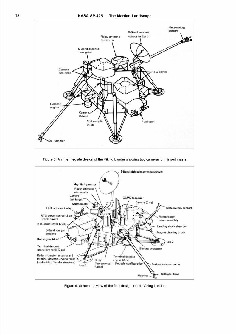
Figure 9. Schematic view of the final design for the Viking Lander.
NASA SP-425 — The Martian Landscape18
8/8/2019 The Martian Landscape
http://slidepdf.com/reader/full/the-martian-landscape 19/160
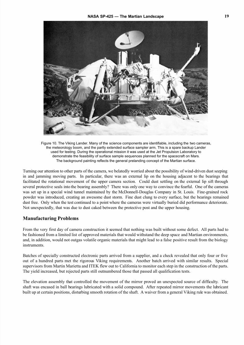
Figure 10. The Viking Lander. Many of the science components are identifiable, including the two cameras,
the meteorology boom, and the partly extended surface sampler arm. This is a spare backup Lander
used for testing. During the operational mission it was used at the Jet Propulsion Laboratory to
demonstrate the feasibility of surface sample sequences planned for the spacecraft on Mars.
The background painting reflects the general prelanding concept of the Martian surface.
Turning our attention to other parts of the camera, we belatedly worried about the possibility of wind-driven dust seeping
in and jamming moving parts. In particular, there was an external lip on the housing adjacent to the bearings that
facilitated the rotational movement of the upper camera section. Could dust settling on the external lip sift throughseveral protective seals into the bearing assembly? There was only one way to convince the fearful. One of the cameras
was set up in a special wind tunnel maintained by the McDonnell-Douglas Company in St. Louis. Fine-grained rock
powder was introduced, creating an awesome dust storm. Fine dust clung to every surface, but the bearings remained
dust free. Only when the test continued to a point where the cameras were virtually buried did performance deteriorate.
Not unexpectedly, that was due to dust caked between the protective post and the upper housing.
Manufacturing Problems
From the very first day of camera construction it seemed that nothing was built without some defect. All parts had to
be fashioned from a limited list of approved materials that would withstand the deep space and Martian environments
and, in addition, would not outgas volatile organic materials that might lead to a false positive result from the biologyinstruments.
Batches of specially constructed electronic parts arrived from a supplier, and a check revealed that only four or five
out of a hundred parts met the rigorous Viking requirements. Another batch arrived with similar results. Special
supervisors from Martin Marietta and ITEK flew out to California to monitor each step in the construction of the parts
The yield increased, but rejected parts still outnumbered those that passed all qualification tests.
The elevation assembly that controlled the movement of the mirror proved an unexpected source of difficulty. The
shaft was encased in ball bearings lubricated with a solid compound. After repeated mirror movements the lubricant
built up at certain positions, disturbing smooth rotation of the shaft. A waiver from a general Viking rule was obtained.
NASA SP-425 — The Martian Landscape 19
8/8/2019 The Martian Landscape
http://slidepdf.com/reader/full/the-martian-landscape 20/160
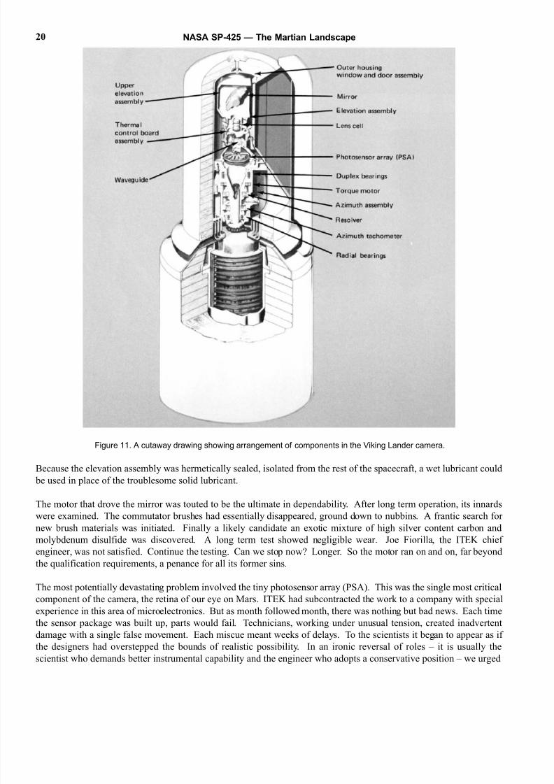
Figure 11. A cutaway drawing showing arrangement of components in the Viking Lander camera.
Because the elevation assembly was hermetically sealed, isolated from the rest of the spacecraft, a wet lubricant could
be used in place of the troublesome solid lubricant.
The motor that drove the mirror was touted to be the ultimate in dependability. After long term operation, its innards
were examined. The commutator brushes had essentially disappeared, ground down to nubbins. A frantic search for
new brush materials was initiated. Finally a likely candidate an exotic mixture of high silver content carbon and
molybdenum disulfide was discovered. A long term test showed negligible wear. Joe Fiorilla, the ITEK chief
engineer, was not satisfied. Continue the testing. Can we stop now? Longer. So the motor ran on and on, far beyondthe qualification requirements, a penance for all its former sins.
The most potentially devastating problem involved the tiny photosensor array (PSA). This was the single most critical
component of the camera, the retina of our eye on Mars. ITEK had subcontracted the work to a company with special
experience in this area of microelectronics. But as month followed month, there was nothing but bad news. Each time
the sensor package was built up, parts would fail. Technicians, working under unusual tension, created inadvertent
damage with a single false movement. Each miscue meant weeks of delays. To the scientists it began to appear as if
the designers had overstepped the bounds of realistic possibility. In an ironic reversal of roles – it is usually the
scientist who demands better instrumental capability and the engineer who adopts a conservative position – we urged
NASA SP-425 — The Martian Landscape20
8/8/2019 The Martian Landscape
http://slidepdf.com/reader/full/the-martian-landscape 21/160
the project engineers to incorporate a simpler photosensor array using only half the diodes. Fortunately our suggestion
was shelved. The struggle went on, but time was running out.
At a tense meeting attended by all the chief managers of the Viking Project, an extraordinary decision was made. The
contract with the ITEK supplier would be terminated, and all partly fabricated components would be sent directly to
the Martin Marietta facility in Denver. There a special laboratory would be equipped to accomplish the work that had
so far defied completion. Bizarre, inverted contractual relationships were forged to fit the special circumstances
NASA Langley built parts for the PSA and supplied them to Martin Marietta. That company built the PSA andfurnished the units to ITEK. ITEK incorporated the PSAs into cameras and delivered them to Martin Marietta under
the Viking contract let by NASA Langley.
It was a hazardous gamble. Important weeks were lost while the new Martin Marietta facility was prepared
Institutional rivalries were ignored – anyone who could help was called in. Bill Patterson, our team engineer with
special background in this area of microelectronics, traveled from Brown University to Denver for a few days of
consultation. Those days stretched into weeks; six months later he returned to Brown. Amazingly, by the time Bill was
back at Brown, the photosensor arrays had been built. And they worked. A few months previously we would have
settled for an array with one or two diodes inoperative. The components delivered to ITEK by the Martin Marietta task
force were completely functional. Several units were shuttled back and forth between Denver and Boston for repair
but, at the time of final camera assembly, every diode in every assembly was ready to carry out its assigned task.
Early on, Viking managers at Langley devised a humbling technique for charting the progress of the program. The
most grievous problems were assigned to the “Top Ten.” At regular weekly reviews, the engineer with relevant
responsibility was required to brief Jim Martin, Project Manager, on what progress had been made. More often than
not, progress was backward.
Barely a year after the start of camera construction Glenn Taylor called me with the expected news – we had made the
Top Ten. We tried to look on the bright side at least we wouldn’t be laboring in darkness anymore. In fact, our early
arrival on the Top Ten (something of a misnomer since the specially designated problems sometimes numbered up to
fifteen) proved beneficial. We received helpful attention from a group of consulting engineers appropriately called the
Tiger Team – before they were exhausted by the endless succession of problems that came later.
The burden of manufacturing problems was especially heavy for the several Martin Marietta engineers who were
permanently in residence at ITEK, coordinating contractual and technical affairs between the two companies. On the
one hand, they were the daily recipients of strident phone messages from their home institution, asking them what the
hell was going on, why nothing was being delivered on time and within cost. On the other hand, the ITEK personnel
were less than delighted with the intrusions of outside observers – they recognized their problems clearly enough,
without having others remind them of their deficiencies.
Vince Corbett was in charge of the Martin Marietta resident group at ITEK. One Friday afternoon, as I sat in his office
listening to tales of misfortune, I urged him to take a day off. Why not drive down to Providence the ITEK facilities
were in nearby Boston – and spend the day sailing on Narragansett Bay? Vince accepted. He, his teenage son, and I
spent a relaxing afternoon on our day sailer. It was one of those lovely crisp Indian summer days. Returning to the
mooring, I made a poor approach. As the buoy drifted by to one side, Vince’s son dove into the cold water to retrieveit. Somehow it seemed an appropriate end to our day of recreation – our mere association with Viking guaranteed that
we would be dogged by misfortune.
One of the more vexing problems proved to have an unexpectedly simple solution. When the camera was operated in
a special chamber cooled to the low temperatures prevailing on the surface of Mars the azimuthal drive jammed. When
the temperature was raised the problem disappeared. Exotic electronic malfunctions were hypothesized, but common
sense observations indicated the real problem. There was very little clearance between the upper camera housing and
the fixed post against which the recessed window was stowed when the camera was not in use. As the temperature
was lowered the post flexed and pressed against the upper housing. The clearance between post and housing was
adjusted slightly and the problem never recurred.
NASA SP-425 — The Martian Landscape 21
8/8/2019 The Martian Landscape
http://slidepdf.com/reader/full/the-martian-landscape 22/160
Gradually, imperceptibly, the situation improved. The final fabrication of the cameras was accomplished virtually
without incident. There were even a few moments of humor. A technician, carefully applying solder to an electrical
junction, looked up to see a group of 18 visiting engineers and administrators standing around his workbench. The
technician, unimpressed, remarked to the ITEK guide that it reminded him of the typical Viking philosophy – one
person does the work and 18 others kibitz.
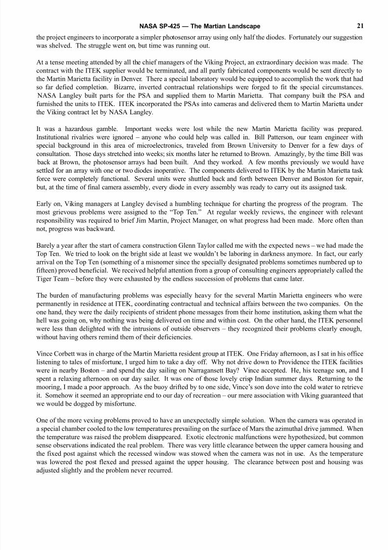
Figure 12. Members of the ITEK team dramatizing (some persons might say overdramatizing)
an important event – delivery of the first camera to Martin Marietta. The upper and
lower camera housings are distinguishable. The fixed post, attached to the top
of the lower housing, is situated to the right of the recessed camera window.
Cameras Without Pictures
During the first years of camera development we found ourselves in the uncomfortable position of judging a
complicated piece of equipment, partly assembled, that had not yet performed its primary function of taking a picture.
As our anxiety increased, a difference of opinion emerged between scientists and engineers. Some, though by no
means all, engineers argued that the capability of the camera could be measured quantitatively only by a series of tests
involving such features as precision of pixel spacing and electrical response of photosensors. The results of the testswere generally shown as tables of figures or graphs. In terms of the contractual requirements, pictures were of little
value. Only in a qualitative way did they demonstrate that the numerically defined specifications had been met.
As I pored over the dryly legal requirements of the contract under which ITEK was working, nowhere could I find reference
to pictures. My engineer friends sought to reassure me. If each of the components performed according to specifications,
a perfect picture must necessarily be the integrated result. I remained skeptical, partly because of my ignorance I was
frustrated by schematic drawings and complicated calculations which I only dimly understood. To the hard-working
engineers, already immersed in more substantial problems such as components that simply would not work, I must have
seemed like the small boy who refuses to believe the Earth is round unless he can travel its complete circumference.
NASA SP-425 — The Martian Landscape22
8/8/2019 The Martian Landscape
http://slidepdf.com/reader/full/the-martian-landscape 23/160
The more the engineers temporized, the more obdurate I became. My resolve was strengthened as others joined the
chorus. Finally, at the start of one of our program review meetings, the announcement was made that a picture would
be distributed at the conclusion – no doubt an inducement calculated to keep us awake through the technical reports.
As that first imperfect image was passed around the table for inspection (Figure 13), the presenter began an apologetic
“Let me explain . . .” The questions were sharp and numerous. What caused the shading variations? Why were some
lines offset? Was this the best spatial resolution we could expect?
The same scene was destined to be repeated many times as the camera design was refined and the manufactureundertaken. For the ITEK engineers it was a choice between the frying pan and the fire. If they failed to produce a
recently acquired picture, scientists and supervisors imagined the worst – the end-to-end camera system didn’t work.
If they did distribute a picture, then every defect was noted, generally with caustic remarks about the cost of the camera
and the quality of the image.
Charlie Ross, the ITEK Program Manager, patiently tried to explain that the defects were a consequence of working
with a prototype model instead of the actual flight cameras. He reminded us that the cameras were designed to take
pictures on Mars, not under the uneven illumination conditions of the laboratory. His protestations sounded weak then,
but we doubting Thomases appreciate now that he was right. Jim Martin, Project Manager, probably had some of those
early ragged pictures in mind when he said, after viewing the first pictures from the surface of Mars, that the cameras
had never worked that well on Earth. Strictly speaking, of course, this was not true, but the apparent difference in
quality was dramatic.
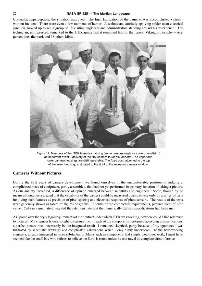
Figure 13. The first panorama taken with the Viking camera, a view of the ITEK parking lot in Lexington, Mass.
The several vertical streaks, indicated by arrows, are not defects. They are the greatly distorted images of cars
that drove by while the picture was being taken.
The first extensive science test of the camera was conducted in August 1971. We used a prototype camera
picturesquely referred to, in engineering parlance, as a breadboard model. To the considerable amusement of lTEK
personnel, several of my graduate students arrived at the camera facility with a box, one meter square, filled with
sediment and rocks. Naturally enough it was irreverently known as Mutch’s sandbox. We took pictures of
assemblages of sand and rocks both with the Viking camera and with a conventional film camera. To our delight wediscovered that many diagnostic features were visible in Viking camera pictures (Figure 14). The images were marred
by vertical banding and line mismatch, but these were problems with identified solutions.
The most important science test occurred in August 1974. By this time the camera manufacture was almost complete
Several units had been delivered to the Martin Marietta facilities in Denver where, eventually, they would be
incorporated in the Lander. For several weeks we scientists were permitted the use of one of the extra cameras that
because of minor manufacturing defects, seemed least likely to be designated for the flight to Mars. (This is a continual
problem for spacecraft experimenters. The best units are always carefully protected from excessive use.) After months
of preliminary campaigning, we were finally granted permission to take the cameras a short distance outdoors, several
hundred yards from the Martin Marietta buildings.
NASA SP-425 — The Martian Landscape 23
8/8/2019 The Martian Landscape
http://slidepdf.com/reader/full/the-martian-landscape 24/160
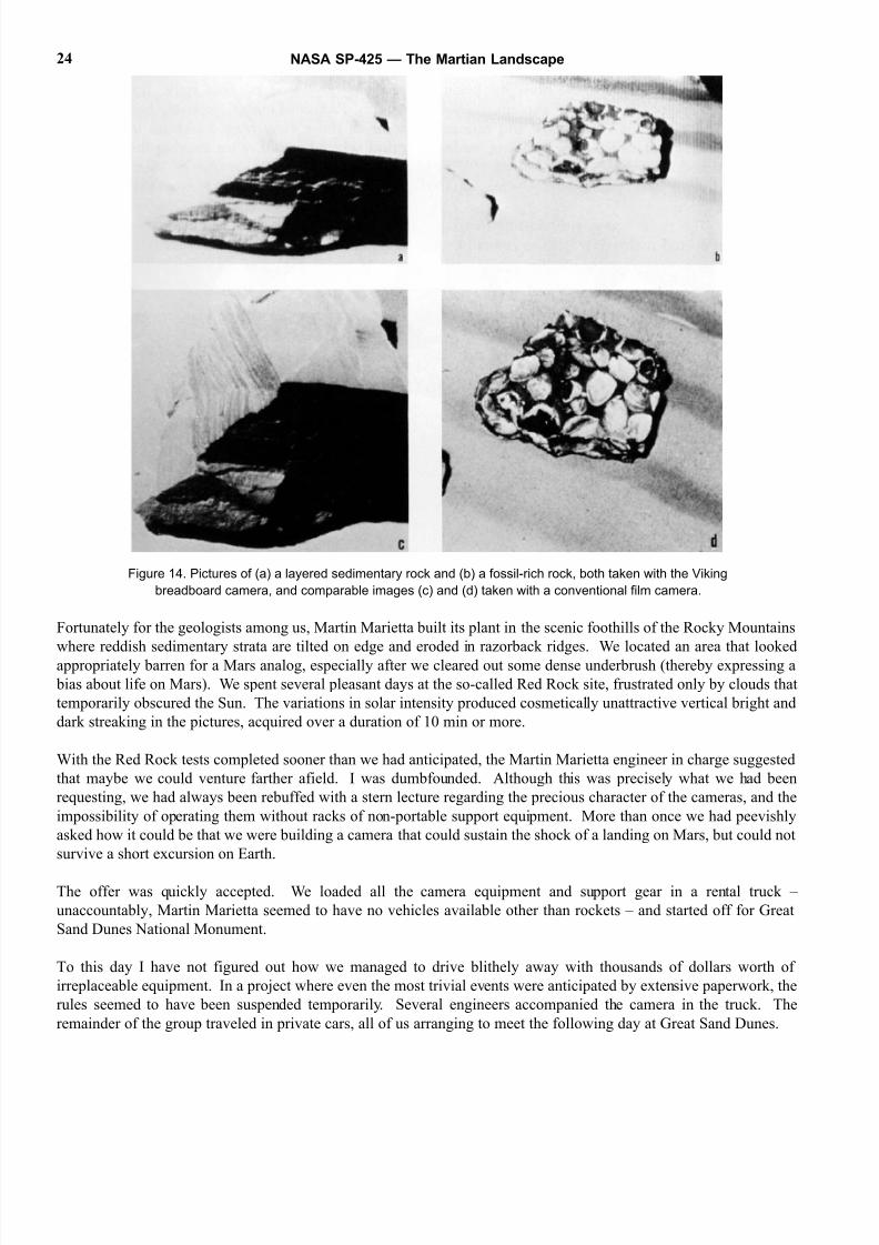
Figure 14. Pictures of (a) a layered sedimentary rock and (b) a fossil-rich rock, both taken with the Viking
breadboard camera, and comparable images (c) and (d) taken with a conventional film camera.
Fortunately for the geologists among us, Martin Marietta built its plant in the scenic foothills of the Rocky Mountains
where reddish sedimentary strata are tilted on edge and eroded in razorback ridges. We located an area that lookedappropriately barren for a Mars analog, especially after we cleared out some dense underbrush (thereby expressing a
bias about life on Mars). We spent several pleasant days at the so-called Red Rock site, frustrated only by clouds that
temporarily obscured the Sun. The variations in solar intensity produced cosmetically unattractive vertical bright and
dark streaking in the pictures, acquired over a duration of 10 min or more.
With the Red Rock tests completed sooner than we had anticipated, the Martin Marietta engineer in charge suggested
that maybe we could venture farther afield. I was dumbfounded. Although this was precisely what we had been
requesting, we had always been rebuffed with a stern lecture regarding the precious character of the cameras, and the
impossibility of operating them without racks of non-portable support equipment. More than once we had peevishly
asked how it could be that we were building a camera that could sustain the shock of a landing on Mars, but could not
survive a short excursion on Earth.
The offer was quickly accepted. We loaded all the camera equipment and support gear in a rental truck –
unaccountably, Martin Marietta seemed to have no vehicles available other than rockets – and started off for Great
Sand Dunes National Monument.
To this day I have not figured out how we managed to drive blithely away with thousands of dollars worth of
irreplaceable equipment. In a project where even the most trivial events were anticipated by extensive paperwork, the
rules seemed to have been suspended temporarily. Several engineers accompanied the camera in the truck. The
remainder of the group traveled in private cars, all of us arranging to meet the following day at Great Sand Dunes.
NASA SP-425 — The Martian Landscape24
8/8/2019 The Martian Landscape
http://slidepdf.com/reader/full/the-martian-landscape 25/160
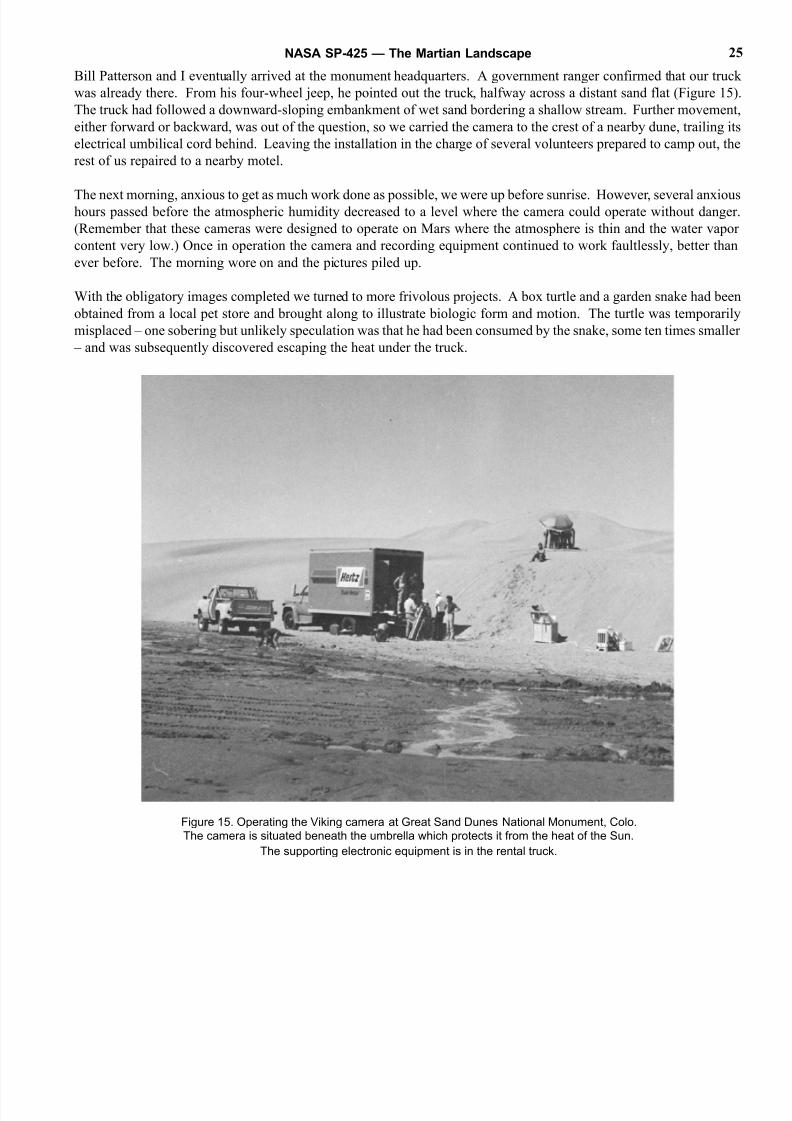
Bill Patterson and I eventually arrived at the monument headquarters. A government ranger confirmed that our truck
was already there. From his four-wheel jeep, he pointed out the truck, halfway across a distant sand flat (Figure 15)
The truck had followed a downward-sloping embankment of wet sand bordering a shallow stream. Further movement
either forward or backward, was out of the question, so we carried the camera to the crest of a nearby dune, trailing its
electrical umbilical cord behind. Leaving the installation in the charge of several volunteers prepared to camp out, the
rest of us repaired to a nearby motel.
The next morning, anxious to get as much work done as possible, we were up before sunrise. However, several anxioushours passed before the atmospheric humidity decreased to a level where the camera could operate without danger
(Remember that these cameras were designed to operate on Mars where the atmosphere is thin and the water vapor
content very low.) Once in operation the camera and recording equipment continued to work faultlessly, better than
ever before. The morning wore on and the pictures piled up.
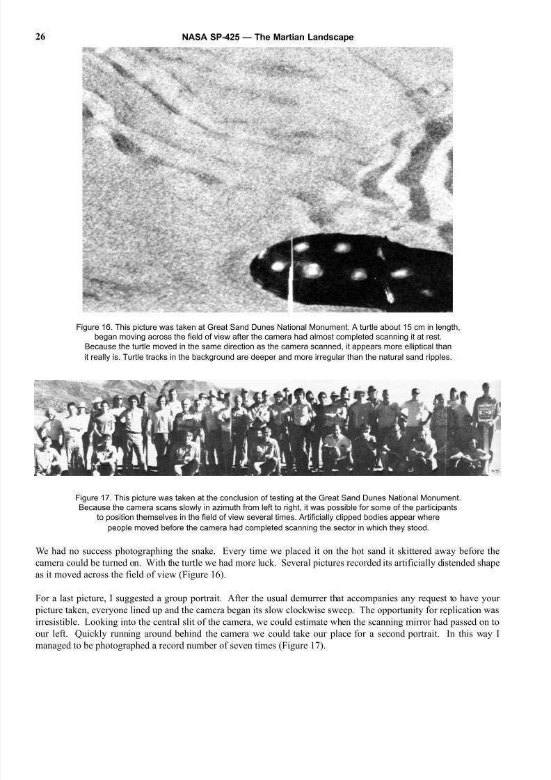
With the obligatory images completed we turned to more frivolous projects. A box turtle and a garden snake had been
obtained from a local pet store and brought along to illustrate biologic form and motion. The turtle was temporarily
misplaced – one sobering but unlikely speculation was that he had been consumed by the snake, some ten times smaller
– and was subsequently discovered escaping the heat under the truck.
Figure 15. Operating the Viking camera at Great Sand Dunes National Monument, Colo.
The camera is situated beneath the umbrella which protects it from the heat of the Sun.
The supporting electronic equipment is in the rental truck.
NASA SP-425 — The Martian Landscape 25
8/8/2019 The Martian Landscape
http://slidepdf.com/reader/full/the-martian-landscape 26/160
Figure 16. This picture was taken at Great Sand Dunes National Monument. A turtle about 15 cm in length,
began moving across the field of view after the camera had almost completed scanning it at rest.
Because the turtle moved in the same direction as the camera scanned, it appears more elliptical than
it really is. Turtle tracks in the background are deeper and more irregular than the natural sand ripples.
Figure 17. This picture was taken at the conclusion of testing at the Great Sand Dunes National Monument.
Because the camera scans slowly in azimuth from left to right, it was possible for some of the participants
to position themselves in the field of view several times. Artificially clipped bodies appear where
people moved before the camera had completed scanning the sector in which they stood.
We had no success photographing the snake. Every time we placed it on the hot sand it skittered away before the
camera could be turned on. With the turtle we had more luck. Several pictures recorded its artificially distended shape
as it moved across the field of view (Figure 16).
For a last picture, I suggested a group portrait. After the usual demurrer that accompanies any request to have your
picture taken, everyone lined up and the camera began its slow clockwise sweep. The opportunity for replication was
irresistible. Looking into the central slit of the camera, we could estimate when the scanning mirror had passed on to
our left. Quickly running around behind the camera we could take our place for a second portrait. In this way I
managed to be photographed a record number of seven times (Figure 17).
NASA SP-425 — The Martian Landscape26
8/8/2019 The Martian Landscape
http://slidepdf.com/reader/full/the-martian-landscape 27/160
That evening we convened in a local restaurant for a celebration banquet. It had been perhaps the happiest day we spent
on the Viking Project prior to the spacecraft’s arrival at Mars. After years of ambiguous tests and reports, we had
certified that the cameras really worked. Putting esoteric calculations and graphs to one side, we had said simply “I want
to take a picture of that.” And each time we asked – close to a hundred times – the camera faultlessly responded.
In a subtle way the success of that day’s testing influenced our attitude toward the entire mission. If the cameras worked
so well, perhaps it was not unreasonable to assume that other spacecraft instruments and components, plagued by
manufacturing problems, might ultimately work just as well. Maybe the reams of paper outlining spacecraft performancehad described reality. Maybe, two years hence, we would actually be looking at pictures from the surface of Mars.
From that point on, the testing of the cameras proceeded without incident.
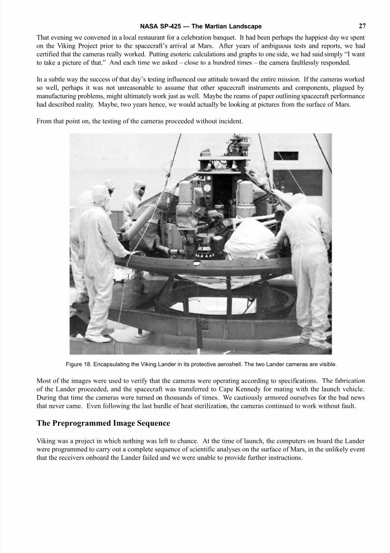
Figure 18. Encapsulating the Viking Lander in its protective aeroshell. The two Lander cameras are visible.
Most of the images were used to verify that the cameras were operating according to specifications. The fabrication
of the Lander proceeded, and the spacecraft was transferred to Cape Kennedy for mating with the launch vehicle.During that time the cameras were turned on thousands of times. We cautiously armored ourselves for the bad news
that never came. Even following the last hurdle of heat sterilization, the cameras continued to work without fault.
The Preprogrammed Image Sequence
Viking was a project in which nothing was left to chance. At the time of launch, the computers on board the Lander
were programmed to carry out a complete sequence of scientific analyses on the surface of Mars, in the unlikely event
that the receivers onboard the Lander failed and we were unable to provide further instructions.
NASA SP-425 — The Martian Landscape 27
8/8/2019 The Martian Landscape
http://slidepdf.com/reader/full/the-martian-landscape 28/160
Consistent with this requirement, we programmed a series of particular pictures to be taken over a 60-sol period (a sol
is a Martian day of 24 hr and 40 min). Hundreds of hours were spent in this elusive exercise how do you best arrange
pictures to document a landscape that you’ve never seen?
We paid little attention to the preprogrammed pictures scheduled late in the mission, but the first two pictures were
planned with care. In the latter case, the preprogrammed images would be the ones actually acquired. Because the
first picture was initiated 25 sec after landing – and the second picture immediately after that – there would be no
opportunity for a change of mind after landing. In any event, the first picture was, by definition, one that could not benefit from prior knowledge of the scene.
The planning for these first two frames was exhaustive. Everyone volunteered advice. More than a year before the
landing, we were summoned to Washington to brief Dr. James Fletcher, NASA administrator, on our camera strategy.
The reason for this unusual attention was obvious. In the event of a botched landing, the first two images might
constitute our only pictorial record of Mars. The pictures would be transmitted to the Orbiter in the first 15 min after
landing, and thence back to Earth. Not for 19 hr – including the passage of a first night on Mars – would it be possible
to communicate again with the Lander.
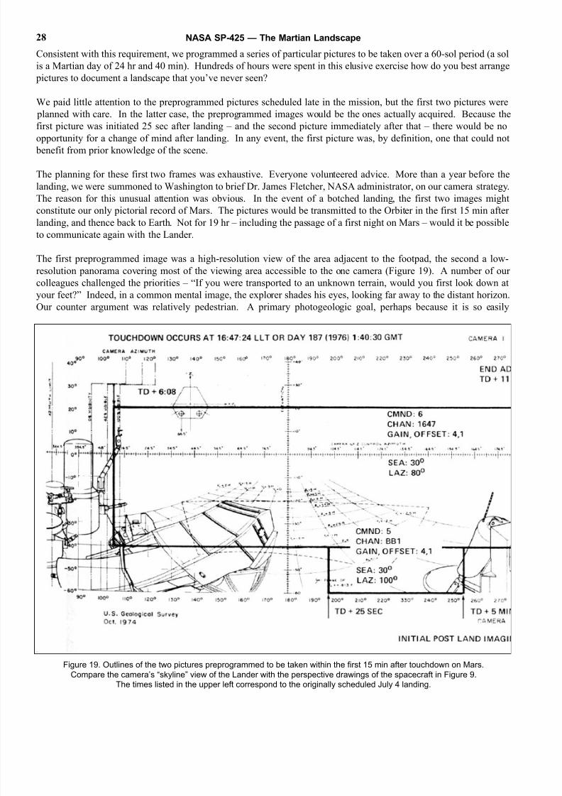
The first preprogrammed image was a high-resolution view of the area adjacent to the footpad, the second a low-
resolution panorama covering most of the viewing area accessible to the one camera (Figure 19). A number of our
colleagues challenged the priorities – “If you were transported to an unknown terrain, would you first look down at
your feet?” Indeed, in a common mental image, the explorer shades his eyes, looking far away to the distant horizon.
Our counter argument was relatively pedestrian. A primary photogeologic goal, perhaps because it is so easily
NASA SP-425 — The Martian Landscape28
Figure 19. Outlines of the two pictures preprogrammed to be taken within the first 15 min after touchdown on Mars.
Compare the camera’s “skyline” view of the Lander with the perspective drawings of the spacecraft in Figure 9.
The times listed in the upper left correspond to the originally scheduled July 4 landing.
8/8/2019 The Martian Landscape
http://slidepdf.com/reader/full/the-martian-landscape 29/160
quantifiable, is increase in linear resolution. Looking nearly straight down, the slant range was about 2 m, yielding a
linear resolution of approximately 2 or 3 mm. Looking toward the horizon, nominally 3 km distant, the linear
resolution would be reduced by three orders of magnitude.
Our logic would have been persuasive if the surface of Mars had been generally flat, but covered with small objects of
unusual form. As it turned out, this was not the case. The rock-littered surface in the near field is relatively
undistinguished, but the undulating topography and diverse geology of the middle and far field is spectacular. From both
an exploratory and scientific perspective, the panorama to the horizon is the more impressive of the first two pictures.
After the Launch
Following two successful launches, the first on August 20, 1975, and the second on September 9, 1975, we looked
forward to a vacation. It seemed that the hard work was over, at least for the next few months. The cameras were on
their way to Mars; we were freed from any more hardware decisions. Commands for the first pictures were
preprogrammed in the Lander computers. What more could we do than sit back and wait during the 10-month journey
to Mars? We soon found out.
The Viking plan called for a mission operations team of more than 800 persons to be in residence at the Jet Propulsion
Laboratory in Pasadena, Calif., directing the spacecraft once they arrived at Mars. The majority of these 800 persons
would be visitors at JPL. Large groups arrived from Martin Marietta and from Langley. Representatives from many
subcontracting companies were on hand to monitor the performance of particular instruments. The scientists, of
course, came from many institutions throughout the country.
NASA SP-425 — The Martian Landscape 29
Figure 19 (continued)
8/8/2019 The Martian Landscape
http://slidepdf.com/reader/full/the-martian-landscape 30/160
It was obvious that there were problems, technical and social, in assuring that this large group worked together
effectively. If everyone dropped in at JPL just a few days before the landing, chaos would result.
The proposed solution was yet another series of tests. All of us were encouraged to be in residence at JPL, starting in
January 1976. I greeted the news with enthusiasm. It seemed a delightful way to escape a New England winter, and
surely there would be ample opportunity for travel and relaxation in southern California. In the months that followed
my wife pointedly reminded me of my prophetic gifts. Between January and November 1976, we had time for just
two weekend trips.
Our first task was strictly bureaucratic. People from many backgrounds had to be blended together in functioning
groups. There were the usual office politics – assignment of office space, secretarial services, and the like. Other
problems were more intriguing. Scientists – especially those working in a university environment – are notoriously
independent. They had no objection to being under the nominal control of group leaders from JPL and Martin
Marietta, but real control was another matter. With their investigations in the balance, they rebelled against the
occasional group leader who attempted to keep all decisions to himself. After a few weeks of job shuffling and
personality testing, we finally settled down to the job at hand.
A series of tests was designed to simulate the actual mission operations. To provide a sense of reality, a group of
“instructors,” working in secrecy, designed a series of mission events that were programmed into the computers.
Accordingly, the computer outputs simulated transmissions from a spacecraft on Mars.
The first test, three days in duration, assumed that things were working well. Our only job was to prepare updated
command loads to respond to specific situations on Mars. We discovered early a frustrating problem that was to plague
us throughout the mission. Any change in the sequence already stored in the Lander computer – even an apparently
minor one – required days, if not weeks, to implement. The reasons were several. First, decision making involved a
pyramidal structure. All decisions initiated at the bottom of the pyramid required approval at higher tiers, in many
cases all the way up to Jim Martin, the Project Manager. Every decision required a meeting. The meetings were
seemingly endless, sometimes even overlapping.
A second problem involved safety. To a degree, operation of any one instrument on the spacecraft jeopardized the
operation of another instrument. Simultaneous operation might result in a power drain or a computer failure. Lessdramatic perils lurked in the background. Designation of a picture somewhat larger than originally planned might
utilize all the recorder tape, leaving no room, for example, for some previously planned biology data.
This maze of interconnected events required an incremental approach. A week or so before a command update was
scheduled, a candidate sequence of events was determined. Then it was run through a preliminary computer program
to detect errors. Inevitably some were found, corrected, and the computer’s approval again requested. Eventually
passing this hurdle, the sequence of events was translated into the special command words that would be transmitted
from giant antennae on Earth to the Lander on Mars. Each final sequence was double checked by using it to operate
a test vehicle on Earth, guaranteeing that the commands produced the desired result.
Clearly, nothing like real-time control of the spacecraft on Mars was possible. Even if there were no other constraint,
the vast Earth-Mars distance meant that it took about 20 min for a radio signal from Earth, traveling at the speed of light, to reach Mars.
The tests became more challenging when anomalies were introduced. Our instructors would simulate some disaster,
leaving it to us to identify and respond to the problem. If our diagnosis was faulty, our corrective surgery clumsy, we
were required to repeat the test. It was like a recurring bad dream come to life. We were back in school, suffering
through final exams.
One anomaly test, simulating the period just before landing, was particularly disconcerting. The problem was
straightforward, but project engineers seemed unwilling to acknowledge transparent truth. The cameras were
scheduled to be turned on, in this way confirming that they were still working after their long trip to Mars. There were
NASA SP-425 — The Martian Landscape30
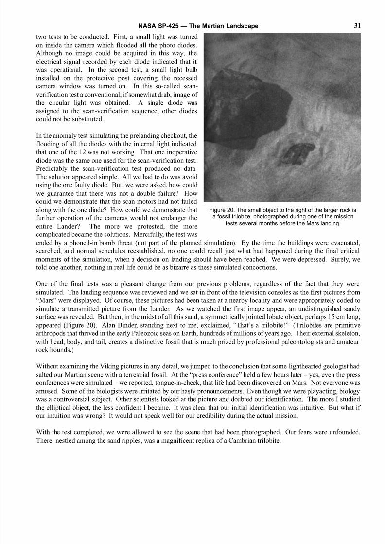
8/8/2019 The Martian Landscape
http://slidepdf.com/reader/full/the-martian-landscape 31/160
two tests to be conducted. First, a small light was turned
on inside the camera which flooded all the photo diodes.
Although no image could be acquired in this way, the
electrical signal recorded by each diode indicated that it
was operational. In the second test, a small light bulb
installed on the protective post covering the recessed
camera window was turned on. In this so-called scan-
verification test a conventional, if somewhat drab, image of the circular light was obtained. A single diode was
assigned to the scan-verification sequence; other diodes
could not be substituted.
In the anomaly test simulating the prelanding checkout, the
flooding of all the diodes with the internal light indicated
that one of the 12 was not working. That one inoperative
diode was the same one used for the scan-verification test.
Predictably the scan-verification test produced no data.
The solution appeared simple. All we had to do was avoid
using the one faulty diode. But, we were asked, how could
we guarantee that there was not a double failure? How
could we demonstrate that the scan motors had not failed
along with the one diode? How could we demonstrate that
further operation of the cameras would not endanger the
entire Lander? The more we protested, the more
complicated became the solutions. Mercifully, the test was
ended by a phoned-in bomb threat (not part of the planned simulation). By the time the buildings were evacuated
searched, and normal schedules reestablished, no one could recall just what had happened during the final critical
moments of the simulation, when a decision on landing should have been reached. We were depressed. Surely, we
told one another, nothing in real life could be as bizarre as these simulated concoctions.
One of the final tests was a pleasant change from our previous problems, regardless of the fact that they weresimulated. The landing sequence was reviewed and we sat in front of the television consoles as the first pictures from
“Mars” were displayed. Of course, these pictures had been taken at a nearby locality and were appropriately coded to
simulate a transmitted picture from the Lander. As we watched the first image appear, an undistinguished sandy
surface was revealed. But then, in the midst of all this sand, a symmetrically jointed lobate object, perhaps 15 cm long
appeared (Figure 20). Alan Binder, standing next to me, exclaimed, “That’s a trilobite!” (Trilobites are primitive
arthropods that thrived in the early Paleozoic seas on Earth, hundreds of millions of years ago. Their external skeleton
with head, body, and tail, creates a distinctive fossil that is much prized by professional paleontologists and amateur
rock hounds.)
Without examining the Viking pictures in any detail, we jumped to the conclusion that some lighthearted geologist had
salted our Martian scene with a terrestrial fossil. At the “press conference” held a few hours later – yes, even the press
conferences were simulated – we reported, tongue-in-cheek, that life had been discovered on Mars. Not everyone wasamused. Some of the biologists were irritated by our hasty pronouncements. Even though we were playacting, biology
was a controversial subject. Other scientists looked at the picture and doubted our identification. The more I studied
the elliptical object, the less confident I became. It was clear that our initial identification was intuitive. But what if
our intuition was wrong? It would not speak well for our credibility during the actual mission.
With the test completed, we were allowed to see the scene that had been photographed. Our fears were unfounded
There, nestled among the sand ripples, was a magnificent replica of a Cambrian trilobite.
NASA SP-425 — The Martian Landscape 31
Figure 20. The small object to the right of the larger rock is
a fossil trilobite, photographed during one of the mission
tests several months before the Mars landing.
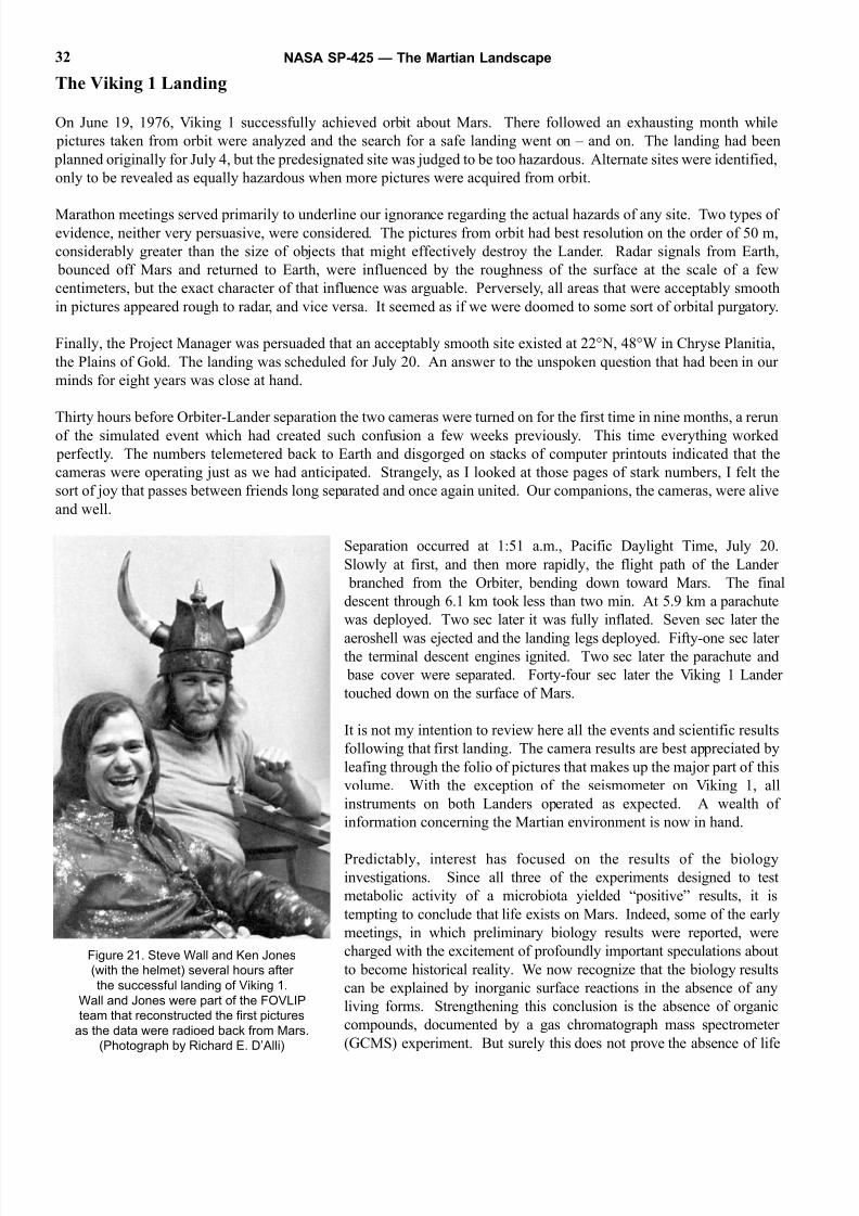
8/8/2019 The Martian Landscape
http://slidepdf.com/reader/full/the-martian-landscape 32/160
The Viking 1 Landing
On June 19, 1976, Viking 1 successfully achieved orbit about Mars. There followed an exhausting month while
pictures taken from orbit were analyzed and the search for a safe landing went on – and on. The landing had been
planned originally for July 4, but the predesignated site was judged to be too hazardous. Alternate sites were identified,
only to be revealed as equally hazardous when more pictures were acquired from orbit.
Marathon meetings served primarily to underline our ignorance regarding the actual hazards of any site. Two types of evidence, neither very persuasive, were considered. The pictures from orbit had best resolution on the order of 50 m,
considerably greater than the size of objects that might effectively destroy the Lander. Radar signals from Earth,
bounced off Mars and returned to Earth, were influenced by the roughness of the surface at the scale of a few
centimeters, but the exact character of that influence was arguable. Perversely, all areas that were acceptably smooth
in pictures appeared rough to radar, and vice versa. It seemed as if we were doomed to some sort of orbital purgatory.
Finally, the Project Manager was persuaded that an acceptably smooth site existed at 22°N, 48°W in Chryse Planitia,
the Plains of Gold. The landing was scheduled for July 20. An answer to the unspoken question that had been in our
minds for eight years was close at hand.
Thirty hours before Orbiter-Lander separation the two cameras were turned on for the first time in nine months, a rerun
of the simulated event which had created such confusion a few weeks previously. This time everything worked
perfectly. The numbers telemetered back to Earth and disgorged on stacks of computer printouts indicated that the
cameras were operating just as we had anticipated. Strangely, as I looked at those pages of stark numbers, I felt the
sort of joy that passes between friends long separated and once again united. Our companions, the cameras, were alive
and well.
Separation occurred at 1:51 a.m., Pacific Daylight Time, July 20.
Slowly at first, and then more rapidly, the flight path of the Lander
branched from the Orbiter, bending down toward Mars. The final
descent through 6.1 km took less than two min. At 5.9 km a parachute
was deployed. Two sec later it was fully inflated. Seven sec later the
aeroshell was ejected and the landing legs deployed. Fifty-one sec later the terminal descent engines ignited. Two sec later the parachute and
base cover were separated. Forty-four sec later the Viking 1 Lander
touched down on the surface of Mars.
It is not my intention to review here all the events and scientific results
following that first landing. The camera results are best appreciated by
leafing through the folio of pictures that makes up the major part of this
volume. With the exception of the seismometer on Viking 1, all
instruments on both Landers operated as expected. A wealth of
information concerning the Martian environment is now in hand.
Predictably, interest has focused on the results of the biology
investigations. Since all three of the experiments designed to test
metabolic activity of a microbiota yielded “positive” results, it is
tempting to conclude that life exists on Mars. Indeed, some of the early
meetings, in which preliminary biology results were reported, were
charged with the excitement of profoundly important speculations about
to become historical reality. We now recognize that the biology results
can be explained by inorganic surface reactions in the absence of any
living forms. Strengthening this conclusion is the absence of organic
compounds, documented by a gas chromatograph mass spectrometer
(GCMS) experiment. But surely this does not prove the absence of life
NASA SP-425 — The Martian Landscape32
Figure 21. Steve Wall and Ken Jones
(with the helmet) several hours after
the successful landing of Viking 1.
Wall and Jones were part of the FOVLIP
team that reconstructed the first pictures
as the data were radioed back from Mars.
(Photograph by Richard E. D’Alli)
8/8/2019 The Martian Landscape
http://slidepdf.com/reader/full/the-martian-landscape 33/160
on Mars, only its absence at two localities purposely chosen to be bland and featureless. It remains possible perhaps
unlikely, although statistics in this instance have little validity – that life exists elsewhere on Mars in some special
environmental niche – or that it existed millions of years ago.
The First Color Picture
During the first day following the Viking 1 early morning landing we were preoccupied with analysis and release of
the first two pictures which, in quality and content, had greatly exceeded our expectations. Almost 24 hr later, whenthe Orbiter once more passed over the Lander, another picture was relayed to Earth, this one in color.
In contrast to the attention we lavished on planning of the first two black and white pictures, we were dismally
unprepared to reconstruct and analyze the first color picture. In a general way we understood that thorough preflight
calibration of the camera’s spectral sensitivity was mandatory. We also knew that we would need software programs
that efficiently transformed the raw data. What we failed to appreciate were the many subtle problems which
uncorrected, could produce major changes in color. Furthermore, we had no intimation of the immediate and
widespread public interest in the first color products – for example, intuitively corrected color images were shown on
television within 30 min following receipt of data on Earth. Although we struggled to delay the deadline, we were
obliged to release the first color prints within 8 hr after receipt of data.
As previously mentioned, there are three sensors with blue, green, and red filters in the focal plane of the camera.
These record the radiance of the scene in blue, green, and red light. However, the multilayer interference filters used
in the cameras (simpler absorptive emulsion layers would have been degraded by preflight heat sterilization) have very
irregular spectral response. The blue channel, for example, responds slightly but significantly to infrared light. The
extraneous parts of the signal must be subtracted, so that the absolute radiances at three specific wavelengths in the
blue, green, and red are represented. A color print is produced by exposing conventional color film to separately
modulated beams of blue, green, and red laser light, scanning the film with the same geometry employed in the camera.
Preflight calibration of the camera thoroughly characterized the sensitivity of each sensor filter combination.
Qualitative tests indicated that simple normalization of the voltages for the three color channels – disregarding spectra
leaks and displacements – was sufficient to produce reasonable color images. In making that judgment our attention
was generally directed to saturated colors in the natural scene and test target.
When the first color data from Marc were received on Earth, we immediately used the same normalization techniques
to calibrate the image. The result was surprising and disquieting. The entire scene, ground and atmosphere alike, was
bathed in a reddish glow. Unwilling to commit ourselves publicly to this provocative display, we adjusted the
parameters in the calibration program until the sky came out a neutral gray. At the same time, rocks and soil showed
good contrast; the colors seemed reasonable. This was the picture released eight hours after receipt of the data. But
to our chagrin the sky took on a bluish hue during reconstruction and photoreproduction. The media representatives
were delighted with the Earth like colors of the scene.
Meanwhile, continued analysis supported the reality of an orangish tint throughout the scene, the atmospheric color
resulting from small suspended soil particles. Several days after the first release, we distributed a second version, this
time with the sky reddish. Predictably, newspaper headlines of “Martian sky turns from blue to red” were followed by
accounts of scientific fallibility. We smiled painfully when reporters asked us if the sky would turn green in a
subsequent version.
Our work over the past year has demonstrated that, even though the sky will not turn green, there will be nevertheless
a long series of color images, each better than – or at least different from – its predecessor. The initial images were
unnaturally saturated, or rich in chrome. Reducing the saturation makes the scene appear more drab. The reader
should keep in mind that color is defined according to three properties: hue, the characteristic wavelength of the
pigmenting material; saturation, the amount of pigmenting material; and brightness, the admixture of pigmenting
material and gray background. Most persons equate apparent color with hue. However, changes in brightness and
saturation can produce images which appear to be much different in hue.
NASA SP-425 — The Martian Landscape 33
8/8/2019 The Martian Landscape
http://slidepdf.com/reader/full/the-martian-landscape 34/160
More important than correcting for saturation was accounting for spectral “out of band” filter transmittance. In order
to do this it is necessary to examine, for each picture element, reflectances in all six bands, three in visual color and
three in near infrared. The amount of off axis radiance for each channel is estimated by considering the radiance in
the five other channels and developing an integrated spectral solution that satisfactorily accounts for the measured
reflectances in all six channels.
The reader may be thinking that problems of color reconstruction largely could have been circumvented by mounting
on the spacecraft targets of known color. In fact, such an array of color chips was mounted and has been imaged. Wehave discovered that accurate color reconstruction of this target is necessary, but not sufficient for certification of good
color in the natural scene. Errors are not particularly noticeable for saturated colors but become significant at low
values of brightness and saturation.
In summary, the color of the Martian scene, perceived by the necessarily abnormal eyes of Viking, is elusive. In response
to the inevitable question: “Is that exactly how it would look if I were standing on Mars?” a qualified “yes” is in order.
Uplink and Downlink
After the excitement of the first days, our work fell into a regular pattern. Each of the more than 40 persons on the
Imaging Team was specially trained to carry out a specific task. All those months of tests began to pay dividends.
The principal division of work was between “uplink,” preparing commands for new pictures to be telemetered to the
Lander, and “downlink,” processing the pictures that had been returned to Earth.
The uplinkers had the most demanding and tedious job. A new command load had to be prepared and certified
approximately every two days. In one sense, the requirements for change in our preprogrammed sequence were less
than we had imagined. The cameras were working perfectly; there was no need to switch pictures from a faulty
photosensor. Indeed, even the estimated exposure settings, the so called gains and offsets, were generally correct. The
entire Martian scene was of equal interest so the strategy of complete coverage displayed in the preprogrammed
sequence was appropriate for the actual mission.
Most changes in pictures were dictated not by us, but requested by others. Scientists and engineers alike were reluctantto conduct spacecraft operations without a picture to document the event. For example, on sol 2, the sampler arm
jammed in an intermediate position because the arm had not extended far enough to release a locking pin. Although
the corrective procedure was relatively straightforward, it was decided that no further commands would be issued until
we acquired a picture of the sampler arm in its stalled position. A last minute camera sequence was prepared; the
resulting picture documented the suspected failure mode.
Throughout the mission, sampler arms on both Landers proved to be prima donnas. Several times they unexpectedly
stalled in the middle of sample acquisition sequences. Each time, a disabling permanent failure was feared – a
disastrous event since the key scientific instruments inside the Lander depended on the sampler arm to provide Martian
soil. However, a new sequence of commands always brought the sampler arms back to life. This oft repeated sequence
of failure despair success elation imparted a Hollywood movie like aura to the mission – it also heightened the
impression of an “intelligent” robot on Mars.
The requirement to monitor the progress of the sampler arm with repeated pictures had some peripheral benefits. Our
ability to generate commands for new picture sequences on very short notice was verified. As some of us had
expected, the burdensome series of meetings and time consuming cross checks could be abbreviated. With the
feasibility of late commands verified by these Lander health pictures, it was relatively easy to persuade managers that
the same techniques could be used to update science sequences.
Pictures were required not only to certify the condition of the Lander; they were also necessary to document each
sample sequence. First the candidate area had to be stereoscopically imaged to locate rocks and slopes that might
endanger the sampler arm. Special computer driven equipment, constructed by one of our Science Team members, Sid
NASA SP-425 — The Martian Landscape34
8/8/2019 The Martian Landscape
http://slidepdf.com/reader/full/the-martian-landscape 35/160
Liebes, was used for rapid construction of topographic profiles. Then a series of pictures was required during the
sampling operation to document each event: successful deployment of the arm, digging of the hole, delivery of the
sample to the inlet ports on the upper deck of the spacecraft. These were extraordinarily difficult sequences to plan
since the pictures had to be precisely timed to intersperse with the sampler operations.
The downlink activity was equally demanding. Each time a transmission occurred from Lander to Earth, either directly
or through the Orbiter relay, a team of two or three persons monitored the incoming data, made preliminary
adjustments, and transferred the data to magnetic tape, suitable for further processing. As each picture was assembledon the screen you were the first to view this part of Mars. It took no unusual flight of fancy to imagine yourself on the
Martian surface. The effect was heightened during those downlinks late at night or early in the morning when the flight
operations building was deserted, with only a skeleton crew to monitor spacecraft operation and to catalog the data
returning to Earth.
Once the raw data had been received in the FOVLIP area (i.e., First Order Viking Lander Imaging Processing – Viking
acronyms numbered in the thousands, and some conversations seemed to be in a foreign tongue), it was passed on to
the Image Processing Laboratory where the pictures were enhanced to produce the best possible image. Although this
procedure appears questionable, it is in fact entirely appropriate. No detail is introduced into the scene that was not
in fact, recorded by the cameras. Since the raw imaging data were generally of high quality, enhancement was usually
limited to restoring lines of data that had been misplaced during transmission, improving picture contrast, and adding
labels and marginal scales.
Superimposed on the uplink and downlink tasks was a constant succession of science meetings and press conferences.
Scientific data were coming in so rapidly that keeping abreast of each new finding was a hopeless task. We had little
time even to study the pictures we had taken. No sooner was one sequence planned and acquired, than we were in the
midst of the next one. Although the frenzied activity of the first few days subsided, the operation of the mission
continued with around the clock activity that consumed all our resources.
The Viking 2 Landing
Viking 2 went into orbit about Mars on August 7, 1976. Searching for an environment most favorable for a Martian
biota, a decision was made to go to higher latitudes where small amounts of H2O ice might temporarily exist in or below the surface. Once in orbit we were required to land in the vicinity of 48°N.
The entire latitude band was searched. None of the pictures was very reassuring. Concern was heightened by the
awareness that at the first landing site there were several rocks in the vicinity of the Lander that could easily have
destroyed it, had the touchdown point been shifted a few meters. The Project Manager decreed that the second site
should be rock free – or, at least, that persuasive arguments in that direction were mandatory. As in the case of the first
landing, the juggling of potential landing sites was both exhaustive and exhausting. As the landing was delayed, the
optional strategies for site certification and simultaneous operation of four spacecraft became Byzantine in complexity
The final decision to land on September 3 was forced less by objective knowledge that we had found a safe site than
by knowledge that the flight team was running out of steam and time.
Viking 2 was targeted to 48°N, 226°W, a spot in Utopia Planitia. The name, at least, augured success. However, an
undefinable pessimism preceded the second landing, strange in light of the success of Viking 1. We realized, perhaps
how quickly the euphoria of past months could change to criticism and disappointment if the second half of the total
mission were unsuccessful.
The Viking 2 Lander separated from its Orbiter at 12:40 p.m. on September 3. Minutes later, telemetered data from
the Lander to Orbiter abruptly stopped. The cause was uncertain, but the prospects looked dim. It was difficult to
imagine that a serious communication failure essentially at the time of separation was not the expression of a more
fundamental problem. Had the Lander incorrectly separated? Was it perhaps still dangling from the Orbiter? Was it
hurtling toward Mars, out of control?
NASA SP-425 — The Martian Landscape 35

8/8/2019 The Martian Landscape
http://slidepdf.com/reader/full/the-martian-landscape 36/160
Within the hour it was demonstrated that the Orbiter had rolled so that its high gain antenna pointed away from Earth. It
was suspected that the loss of control was due to the failure of an inertial reference power source. Fortunately there was
a redundant power source. By switching to the backup the Orbiter was reoriented, but not until several hours after landing.
Meanwhile, we could track the descent of Viking 2 by using a low gain antenna on the Orbiter to monitor the signals
sent by the Lander. Although little in the way of detailed data was received, the very presence of the Lander signal
meant that it was operational. During an expected communication blackout immediately preceding landing, we
listened as the mission controller called out “Touchdown minus seven, six, five, four, three, two, one, zero.” Therewas a long silence. It seemed like minutes. Over the loudspeaker came a muffled prayer, “Come on, baby.” Nothing.
I looked down at my shoes. I remember thinking, “You always wondered what a failure would feel like. Now you
know.” I mentally composed some remarks for friends standing nearby. Finally, the silence was broken. “We have
touchdown.” Pandemonium broke loose a completely unrestrained celebration unlike the more self conscious
moments following the Viking 1 landing. For a few hours, with regular communication from the Lander still not
established, there was nothing much to be done. Cases of champagne magically appeared. The tight security
procedures were temporarily suspended. Families trooped into the laboratories to share in the excitement. Two
successful landings! It was an outcome that not even the most optimistic had looked forward to.
It was not until late that evening that regular communication with the Orbiter could be established. Now it could relay
the pictures that, almost eight hours previously, had been transmitted from Lander to Orbiter just after touchdown. We
were already exhausted after a long day. The event held little of the drama associated with the first Viking 1 pictures.
Indeed, at first glance, the Viking 2 landscape was something of a disappointment, looking superficially like the Viking
1 scene. The profusion of large blocks was the source of wry amusement. Jim Martin reminded us that we had
promised a landing on undulating desert dunes.
Figure 22. Site certification meeting for Viking 2 landing. (Photograph by Hans Peter Biemann)
In the subsequent weeks I revised my opinion of the Viking 2 site. It is, in fact, quite different from the first site, andthe geological histories are probably dramatically diverse. Nonetheless, as the days passed by, I could feel my
enthusiasm waning, the Viking experience slipping away. I looked forward to the end.
In early November the primary mission concluded. Mars passed behind the Sun and communication with the four
spacecraft was temporarily impossible.
We crossed off the last few days on the calendar, just like the last days of school. The very last night I stayed late at
the laboratory, writing notes to a few of the people with whom I had worked so closely for so long. The next morning
my wife, youngest daughter, and I started off – a roundabout route back to Providence by way of the Sierras. We spent
four days in Yosemite. The valley was virtually deserted this late in the season, the ground thickly covered with crisp
NASA SP-425 — The Martian Landscape36
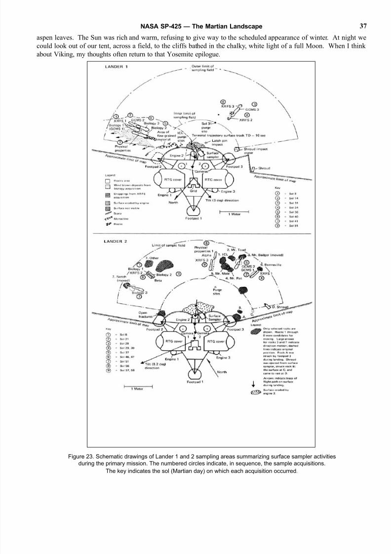
8/8/2019 The Martian Landscape
http://slidepdf.com/reader/full/the-martian-landscape 37/160
aspen leaves. The Sun was rich and warm, refusing to give way to the scheduled appearance of winter. At night we
could look out of our tent, across a field, to the cliffs bathed in the chalky, white light of a full Moon. When I think
about Viking, my thoughts often return to that Yosemite epilogue.
Figure 23. Schematic drawings of Lander 1 and 2 sampling areas summarizing surface sampler activities
during the primary mission. The numbered circles indicate, in sequence, the sample acquisitions.
The key indicates the sol (Martian day) on which each acquisition occurred.
NASA SP-425 — The Martian Landscape 37
8/8/2019 The Martian Landscape
http://slidepdf.com/reader/full/the-martian-landscape 38/160
The Extended Mission
Mars reappeared from behind the Sun, as viewed from Earth in mid-December 1976. This signaled the start of the so-
called extended mission. Communication with all four spacecraft was reestablished. This phase of the mission was
planned to continue through May of 1978, perhaps even longer.
The extended mission illustrates the general proposition that once a demanding problem has been solved – albeit with
great difficulty – the second time is routine. Examples abound in the annals of exploration, particularlymountaineering. So it is with the extended mission. Complicated sequences of trenching and sample acquisition are
carried out without fanfare. Many more pictures have been taken than during the primary mission. Before the Viking
mission is completed we will have monitored the environment for almost a complete Martian year, or one revolution
about the Sun, a total of 687 Earth days. The scientific return is just now being cataloged. It will be years before the
analysis is complete. In that sense, the Viking mission is still in its infancy.
Many of the persons who played an instrumental role in the primary mission have now gone. The new team is no less
competent, but the excitement inevitably has been replaced by a workaday approach. I return to JPL frequently to
examine the most recent collection of pictures, but I feel out of place, like a college graduate who returns to his campus
and finds himself among a new generation, perhaps only a few years younger but still a world apart.
The Future
I was encouraged by a valued editorial advisor to close with a look toward the future. In fact, the events of the future
are blurred. On a personal basis I realize that many of us who worked on Viking will never again be associated with
a comparable journey of space exploration, not because we are in any way disenchanted but because it is time to move
on to other things. That separation is bittersweet. The memories keep popping up at unexpected moments, and present
ventures seem drab by comparison.
As to further unmanned exploration of Mars, preliminary plans exist for a rover mission in the late 1980s. A tractor-
drive vehicle, slightly larger than Viking, could roam up to several hundred kilometers, sampling geological and
biological environments inaccessible to Viking. This might be followed by an unmanned sample-return mission in the
early 1990s, providing the first opportunity to analyze Martian surface materials in great detail. But these missionsexist only on paper. Neither has been approved and their large cost necessarily makes them vulnerable.
Even if the immediate future is uncertain, I have no doubts about the distant years. Some day man will roam the surface
of Mars. Those wonderful Viking machines will be crated up, returned to Earth, and placed in a museum. Children in
generations to come will stand before them and struggle to imagine the way it was on that first journey to Mars.
NASA SP-425 — The Martian Landscape38
8/8/2019 The Martian Landscape
http://slidepdf.com/reader/full/the-martian-landscape 39/160
Viking 1 Lander Pictures
The pictures in this volume were selected and arranged by Kenneth L. Jones who, in addition, was responsible for the
special processing of the original imaging data.
Because the Viking Lander cameras have a fixed vertical field of view of either 20° (high resolution mode) or 60°
(survey, color, and infrared modes), but an adjustable azimuthal dimension, many of the pictures are relatively long
panoramas. In some instances we have been obliged to split these panoramas so that two parts appear on facing pages
Where this has been necessary we have retained a small amount of overlapping image so that the reader can mentally
piece the two parts together.
Individual captions are not intended to be exhaustive descriptions of the pictures. Many objects appear in more than
one picture, but are mentioned only where they are shown to best advantage. All particulars relating to camera settings
time of day, picture location, and the like are contained in the table which appears on page 154. The position and scale
of pictures can be visualized by reference to the skyline drawings that accompany the table. By using this supporting
information, readers can answer for themselves certain technical questions raised by the pictures but not discussed in
the captions.
NASA SP-425 — The Martian Landscape 39
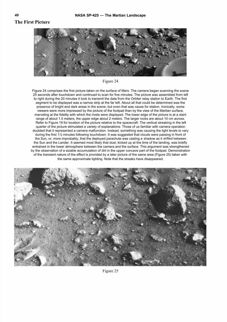
8/8/2019 The Martian Landscape
http://slidepdf.com/reader/full/the-martian-landscape 40/160
The First Picture
Figure 24
Figure 24 comprises the first picture taken on the surface of Mars. The camera began scanning the scene
25 seconds after touchdown and continued to scan for five minutes. The picture was assembled from left
to right during the 20 minutes it took to transmit the data from the Orbiter relay station to Earth. The first
segment to be displayed was a narrow strip at the far left. About all that could be determined was the
presence of bright and dark areas in the scene, but even that was cause for elation. Ironically, some
viewers were more impressed by the picture of the footpad than by the view of the Martian surface,
marveling at the fidelity with which the rivets were displayed. The lower edge of the picture is at a slant
range of about 1.5 meters, the upper edge about 2 meters. The larger rocks are about 10 cm across.
Refer to Figure 19 for location of the picture relative to the spacecraft. The vertical streaking in the left
quarter of the picture stimulated a variety of explanations. Those of us familiar with camera operation
doubted that it represented a camera malfunction. Instead, something was causing the light levels to vary
during the first 1½ minutes following touchdown. It was suggested that clouds were passing in front of
the Sun, or, more improbably, that the deployed parachute was casting a shadow as it drifted between
the Sun and the Lander. It seemed most likely that dust, kicked up at the time of the landing, was briefly
entrained in the lower atmosphere between the camera and the surface. This argument was strengthened
by the observation of a sizable accumulation of dirt in the upper concave part of the footpad. Demonstration
of the transient nature of the effect is provided by a later picture of the same area (Figure 25) taken with
the same approximate lighting. Note that the streaks have disappeared.
Figure 25
NASA SP-425 — The Martian Landscape40
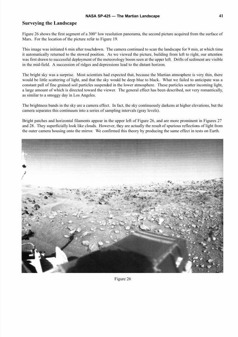
8/8/2019 The Martian Landscape
http://slidepdf.com/reader/full/the-martian-landscape 41/160
Surveying the Landscape
Figure 26 shows the first segment of a 300° low resolution panorama, the second picture acquired from the surface of
Mars. For the location of the picture refer to Figure 19.
This image was initiated 6 min after touchdown. The camera continued to scan the landscape for 9 min, at which time
it automatically returned to the stowed position. As we viewed the picture, building from left to right, our attention
was first drawn to successful deployment of the meteorology boom seen at the upper left. Drifts of sediment are visiblein the mid-field. A succession of ridges and depressions lead to the distant horizon.
The bright sky was a surprise. Most scientists had expected that, because the Martian atmosphere is very thin, there
would be little scattering of light, and that the sky would be deep blue to black. What we failed to anticipate was a
constant pall of fine grained soil particles suspended in the lower atmosphere. These particles scatter incoming light
a large amount of which is directed toward the viewer. The general effect has been described, not very romantically
as similar to a smoggy day in Los Angeles.
The brightness bands in the sky are a camera effect. In fact, the sky continuously darkens at higher elevations, but the
camera separates this continuum into a series of sampling intervals (gray levels).
Bright patches and horizontal filaments appear in the upper left of Figure 26, and are more prominent in Figures 27
and 28. They superficially look like clouds. However, they are actually the result of spurious reflections of light from
the outer camera housing onto the mirror. We confirmed this theory by producing the same effect in tests on Earth.
Figure 26
NASA SP-425 — The Martian Landscape 41
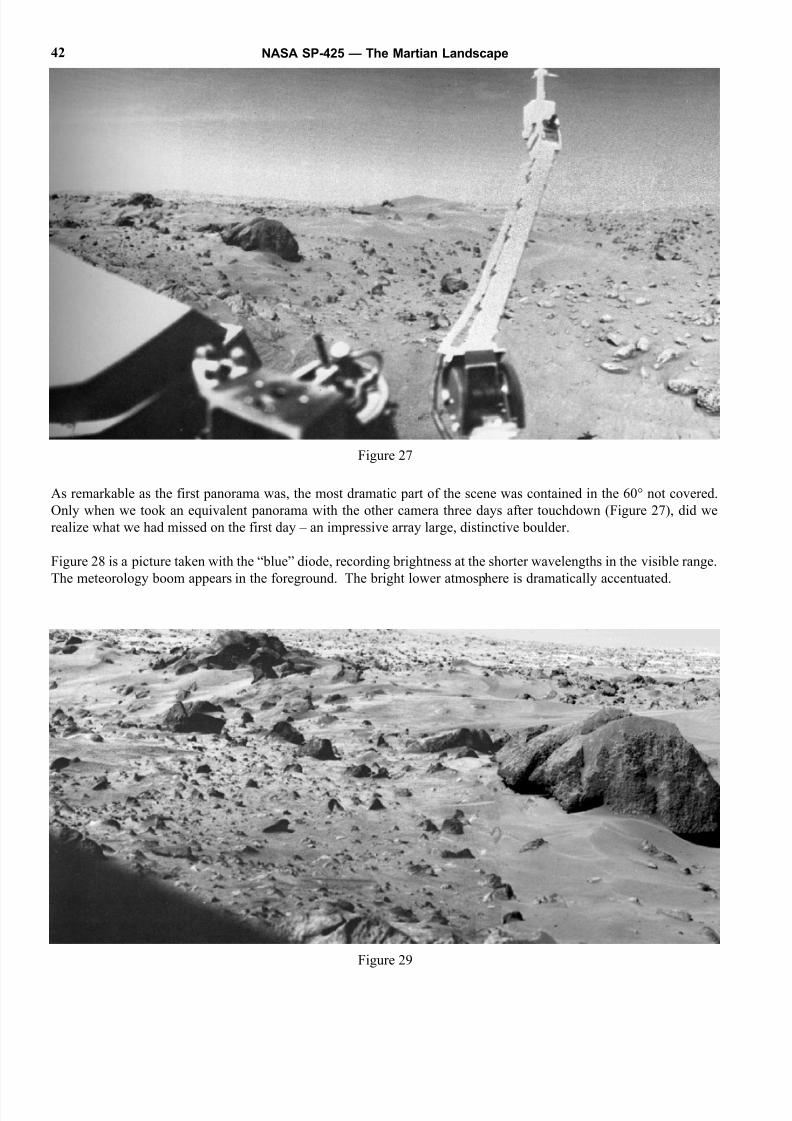
8/8/2019 The Martian Landscape
http://slidepdf.com/reader/full/the-martian-landscape 42/160
As remarkable as the first panorama was, the most dramatic part of the scene was contained in the 60° not covered.
Only when we took an equivalent panorama with the other camera three days after touchdown (Figure 27), did we
realize what we had missed on the first day – an impressive array large, distinctive boulder.
Figure 28 is a picture taken with the “blue” diode, recording brightness at the shorter wavelengths in the visible range.
The meteorology boom appears in the foreground. The bright lower atmosphere is dramatically accentuated.
NASA SP-425 — The Martian Landscape42
Figure 27
Figure 29
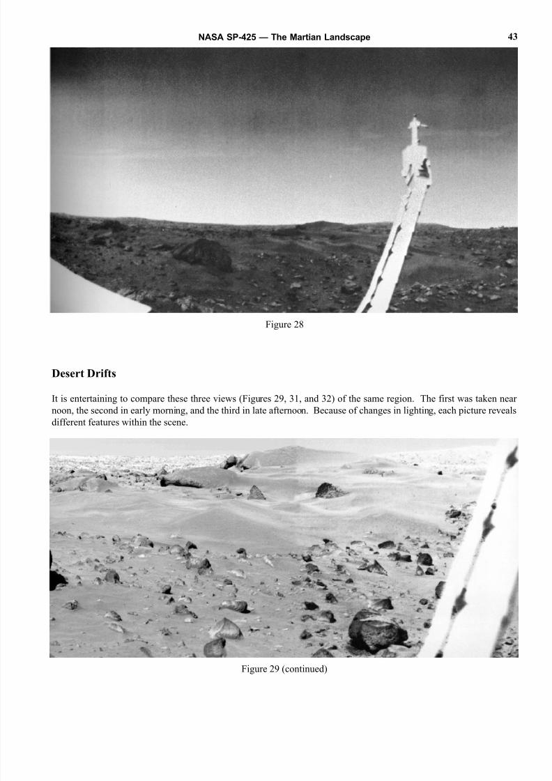
8/8/2019 The Martian Landscape
http://slidepdf.com/reader/full/the-martian-landscape 43/160
Desert Drifts
It is entertaining to compare these three views (Figures 29, 31, and 32) of the same region. The first was taken near
noon, the second in early morning, and the third in late afternoon. Because of changes in lighting, each picture revealsdifferent features within the scene.
NASA SP-425 — The Martian Landscape 43
Figure 29 (continued)
Figure 28
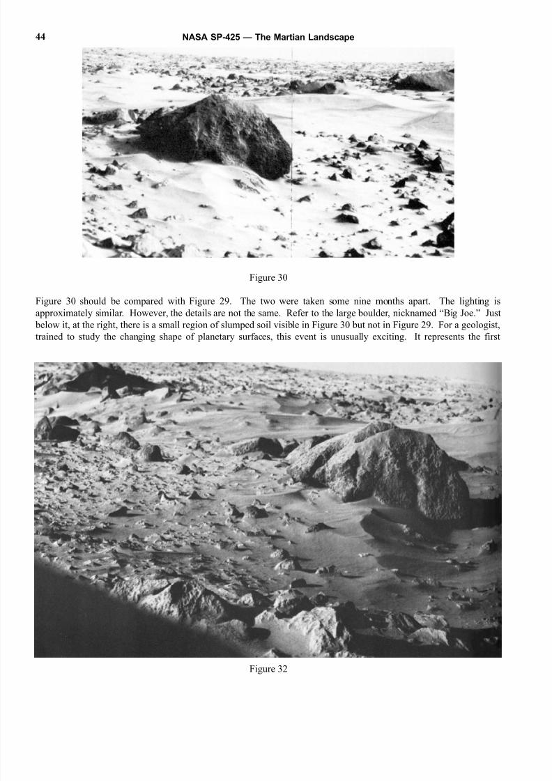
8/8/2019 The Martian Landscape
http://slidepdf.com/reader/full/the-martian-landscape 44/160
Figure 30
Figure 30 should be compared with Figure 29. The two were taken some nine months apart. The lighting is
approximately similar. However, the details are not the same. Refer to the large boulder, nicknamed “Big Joe.” Just
below it, at the right, there is a small region of slumped soil visible in Figure 30 but not in Figure 29. For a geologist,
trained to study the changing shape of planetary surfaces, this event is unusually exciting. It represents the first
NASA SP-425 — The Martian Landscape44
Figure 32
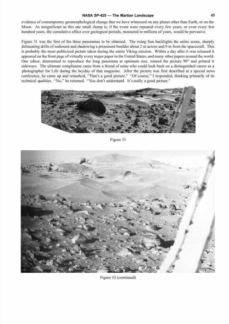
8/8/2019 The Martian Landscape
http://slidepdf.com/reader/full/the-martian-landscape 45/160
evidence of contemporary geomorphological change that we have witnessed on any planet other than Earth, or on the
Moon. As insignificant as this one small slump is, if the event were repeated every few years, or even every few
hundred years, the cumulative effect over geological periods, measured in millions of years, would be pervasive.
Figure 31 was the first of the three panoramas to be obtained. The rising Sun backlights the entire scene, sharply
delineating drifts of sediment and shadowing a prominent boulder about 2 m across and 9 m from the spacecraft. This
is probably the most publicized picture taken during the entire Viking mission. Within a day after it was released it
appeared on the front page of virtually every major paper in the United States, and many other papers around the worldOne editor, determined to reproduce the long panorama at optimum size, rotated the picture 90° and printed it
sideways. The ultimate compliment came from a friend of mine who could look back on a distinguished career as a
photographer for Life during the heyday of that magazine. After the picture was first described at a special new
conference, he came up and remarked, “That’s a good picture.” “Of course,” I responded, thinking primarily of its
technical qualities. “No,” he returned. “You don’t understand. It’s really a good picture.”
Figure 31
NASA SP-425 — The Martian Landscape 45
Figure 32 (continued)

8/8/2019 The Martian Landscape
http://slidepdf.com/reader/full/the-martian-landscape 46/160
The origin of Big Joe has not been established. The rock is coarsely granular and is banded in one, possibly two,
directions. It may be a breccia fragment, thrown out by a nearby meteoroid impact. Supporting this interpretation is
the fact that Big Joe actually is two closely matched boulders side by side. The cleft between the boulders is visible
as a notch in the shadow (Figure 32). The two-boulder occurrence appears more consistent with splitting on impact
than with erosion in place. Also, some analysts have remarked on the apparent ring-like arrangement of small blocks
to the right of Big Joe. However, detailed mapping of the blocks fails to document any circular geometry.
Note that Big Joe is capped with fine-grained material. This may be a remnant of a much thicker cover of dust thatformerly covered the entire region to a depth of several meters.
Sculpted Layers
Figures 33 and 34 are two views of sediment drifts showing internal stratification. At first glance these appear to be
sets of small scale surface ripples. Closer examination reveals that the linear markings result from erosion of a
sequence of sedimentary layers. The same sort of internal stratification can be seen on a seashore beach by trenching
through the sand. On a much grander scale, internal stratification of desert dunes is revealed by erosion of Mesozoic
rocks in the American Southwest, notably in Bryce and Zion National Parks. In Figure 34 the drift at the right of the
image displays several prominent ridges. Darker, more resistant layers are revealed on the eroded drift faces, covered
by a thin layer of brighter material.
The presence of sedimentary layers within the Martian drifts indicates a number of depositional events, each related to
a change in the wind conditions. The exposure of the layers indicates that the most recent event is general erosion. If
these were actively growing dunes the internal stratification would not be revealed.
Four views of isolated drifts of sediment about 20 m to the southeast of Lander 1 are shown in Figures 35 to 38. One
is tempted to call these features sand dunes but the label carries certain implications that cannot be established. First,
the constituent particles probably are not sand, but are finer grained silt and clay. Second, it does not appear that these
are actively growing dunes of the type one commonly associates with deserts. Instead, they appear to be stabilized
erosional remnants of a formerly more extensive sediment cover.
Figure 36 was taken with diode BB 3 (high resolution, focused at 4.5 m). Better definition of distant objects is renderedin Figures 35, 37, and 38, taken with BB 4 (high resolution, focused at 13.3 m). Figures 35 and 37 were taken at
approximately the same early morning hour. Figures 36 and 38 were taken near local noon; Sun elevation is about 50°.
The same dark drift that appears in the upper right of Figures 35 and 36 is situated in the middle of Figures 37 and 38.
A much brighter drift is observable in the upper left of Figures 35 and 36. The difference in brightness (albedo)
suggests a compositional difference. This is substantiated by spectral curves generated from data in the three visible
color and three infrared channels. The shape of the spectral reflection curves indicates that the dark dune is enriched
in ferrous materials, perhaps the mineral magnetite. Pictures acquired much later in the mission, more than a year after
touchdown, show dark patches developing on some bright drifts. This suggests that the bright drifts are, in fact, dark
drifts with a thin veneer of bright fine grained dust. Generally analogous situations occur on Earth where grains of
heavier minerals such as magnetite are preferentially enriched in certain regions where lighter particles of quartz and
feldspar have been swept away by wind.
Near the bottom center in Figure 36 there is a cylinder shaped rock. In early news briefings this was nicknamed the
“Midas Muffler” rock. However, the same rock as viewed in Figure 35 is not so striking – less of a muffler, more of
a garden variety boulder.
The larger boulders on the horizon are about 90 m distant and about 1 to 2 m in diameter. They appear to be eroded
into unusual scalloped shapes, although this may be an illusion rendered by low resolution and high contrast lighting.
Finer sediment is banked up within the boulder cluster. The same association of boulders and accumulation of
sediment occurs elsewhere in the scene. Knobby bedrock is visible in the foreground, and is described in more detail
in the text with Figures 52 through 55.
NASA SP-425 — The Martian Landscape46
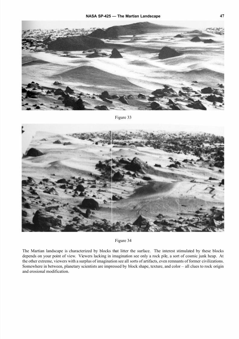
8/8/2019 The Martian Landscape
http://slidepdf.com/reader/full/the-martian-landscape 47/160
Figure 33
Figure 34
The Martian landscape is characterized by blocks that litter the surface. The interest stimulated by these blocks
depends on your point of view. Viewers lacking in imagination see only a rock pile, a sort of cosmic junk heap. At
the other extreme, viewers with a surplus of imagination see all sorts of artifacts, even remnants of former civilizations
Somewhere in between, planetary scientists are impressed by block shape, texture, and color – all clues to rock origin
and erosional modification.
NASA SP-425 — The Martian Landscape 47
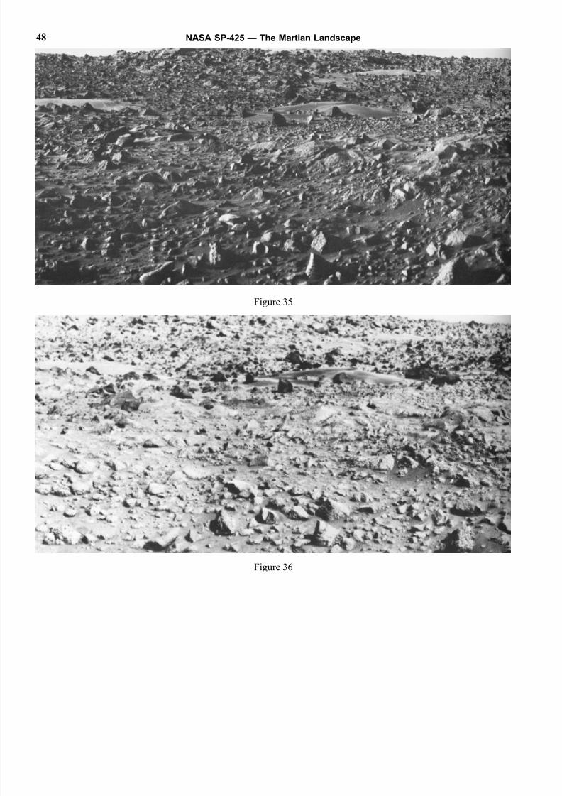
8/8/2019 The Martian Landscape
http://slidepdf.com/reader/full/the-martian-landscape 48/160
Figure 35
Figure 36
NASA SP-425 — The Martian Landscape48
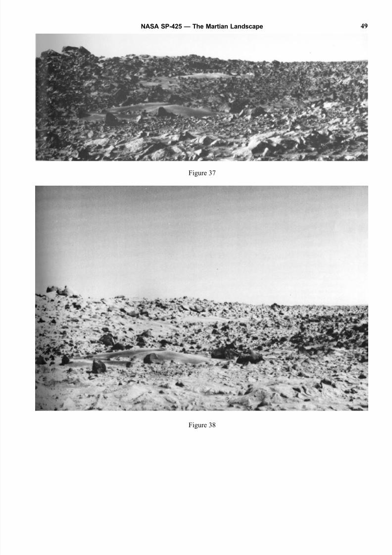
8/8/2019 The Martian Landscape
http://slidepdf.com/reader/full/the-martian-landscape 49/160
Figure 37
Figure 38
NASA SP-425 — The Martian Landscape 49
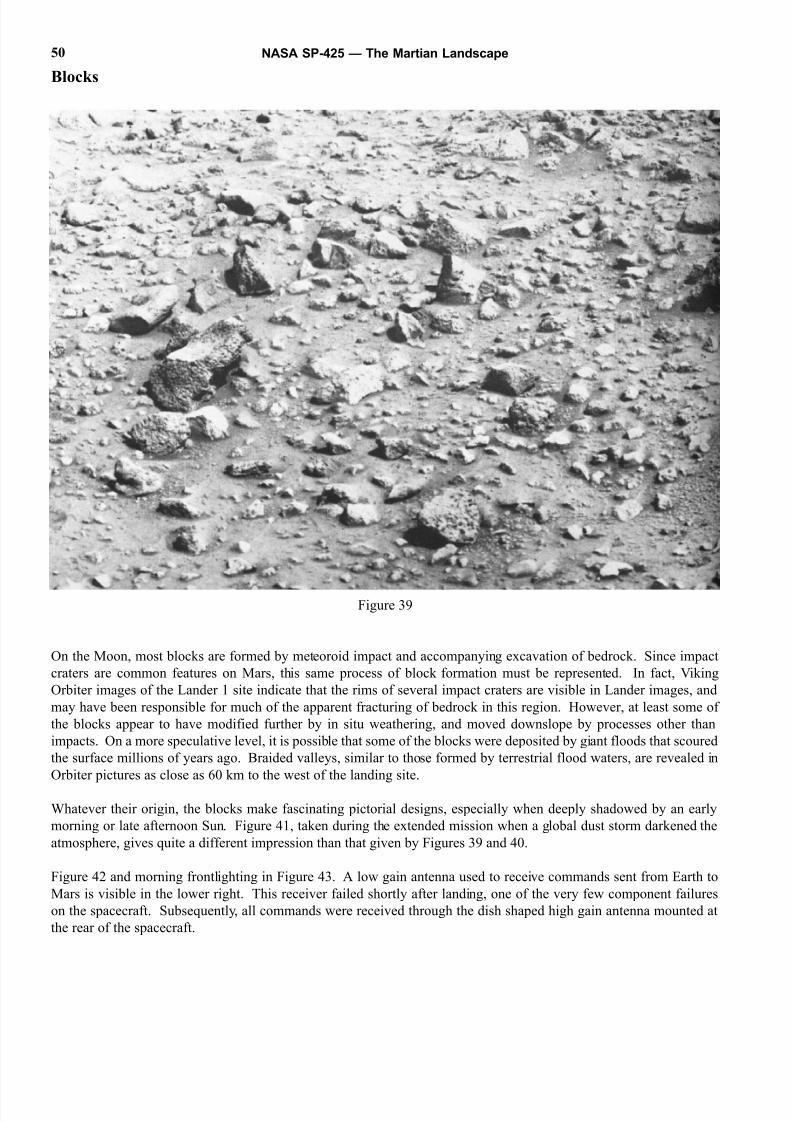
8/8/2019 The Martian Landscape
http://slidepdf.com/reader/full/the-martian-landscape 50/160
Blocks
Figure 39
On the Moon, most blocks are formed by meteoroid impact and accompanying excavation of bedrock. Since impact
craters are common features on Mars, this same process of block formation must be represented. In fact, Viking
Orbiter images of the Lander 1 site indicate that the rims of several impact craters are visible in Lander images, and
may have been responsible for much of the apparent fracturing of bedrock in this region. However, at least some of
the blocks appear to have modified further by in situ weathering, and moved downslope by processes other than
impacts. On a more speculative level, it is possible that some of the blocks were deposited by giant floods that scoured
the surface millions of years ago. Braided valleys, similar to those formed by terrestrial flood waters, are revealed in
Orbiter pictures as close as 60 km to the west of the landing site.
Whatever their origin, the blocks make fascinating pictorial designs, especially when deeply shadowed by an early
morning or late afternoon Sun. Figure 41, taken during the extended mission when a global dust storm darkened the
atmosphere, gives quite a different impression than that given by Figures 39 and 40.
Figure 42 and morning frontlighting in Figure 43. A low gain antenna used to receive commands sent from Earth to
Mars is visible in the lower right. This receiver failed shortly after landing, one of the very few component failures
on the spacecraft. Subsequently, all commands were received through the dish shaped high gain antenna mounted at
the rear of the spacecraft.
NASA SP-425 — The Martian Landscape50
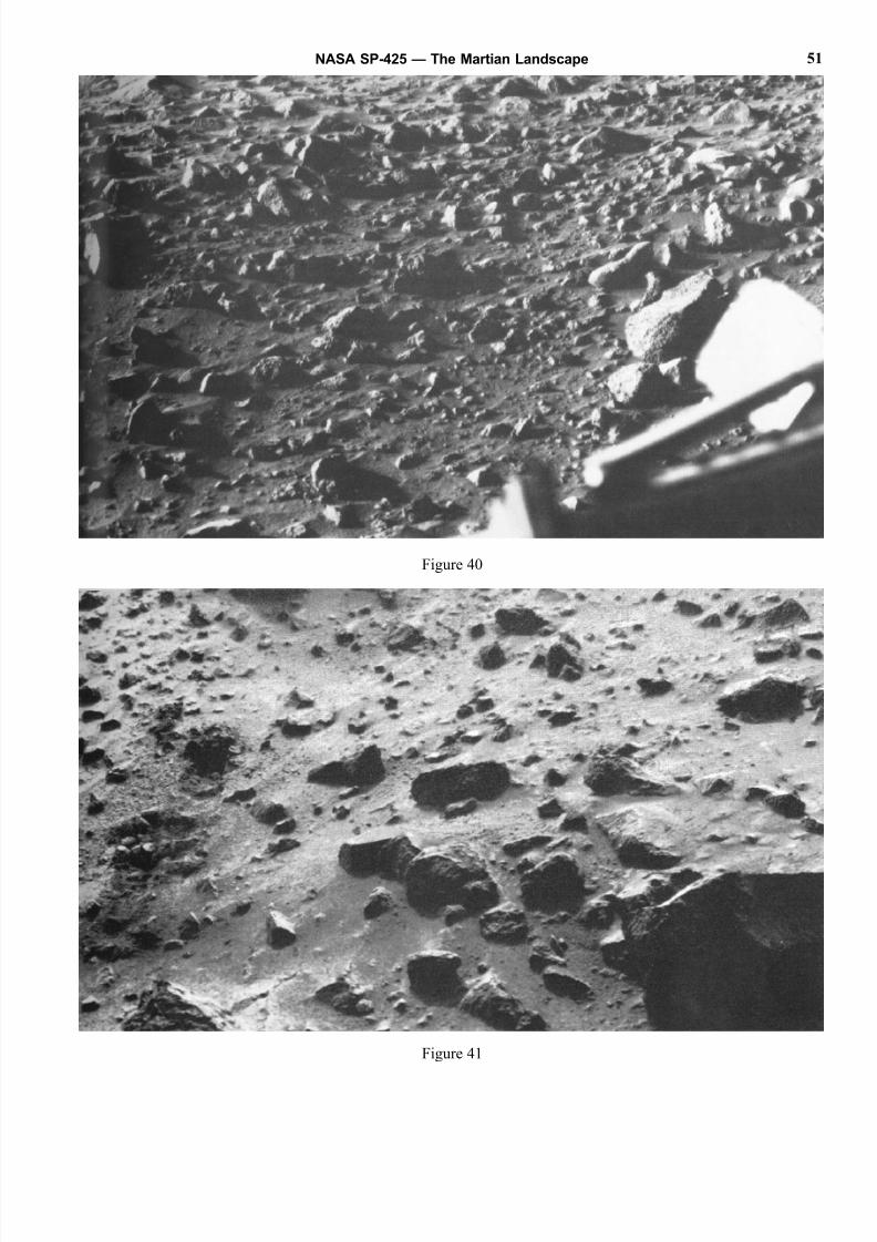
8/8/2019 The Martian Landscape
http://slidepdf.com/reader/full/the-martian-landscape 51/160
Figure 40
Figure 41
NASA SP-425 — The Martian Landscape 51
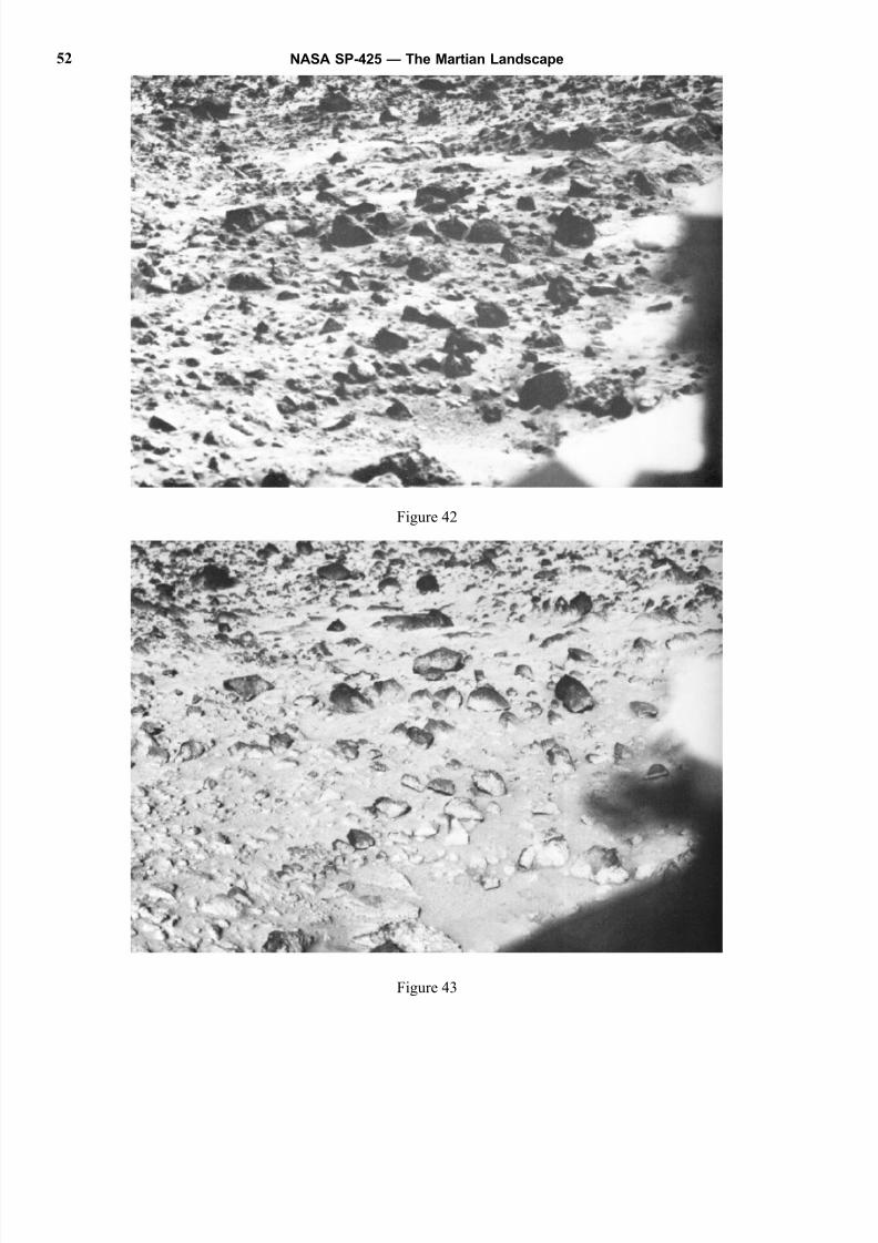
8/8/2019 The Martian Landscape
http://slidepdf.com/reader/full/the-martian-landscape 52/160
Figure 42
Figure 43
NASA SP-425 — The Martian Landscape52
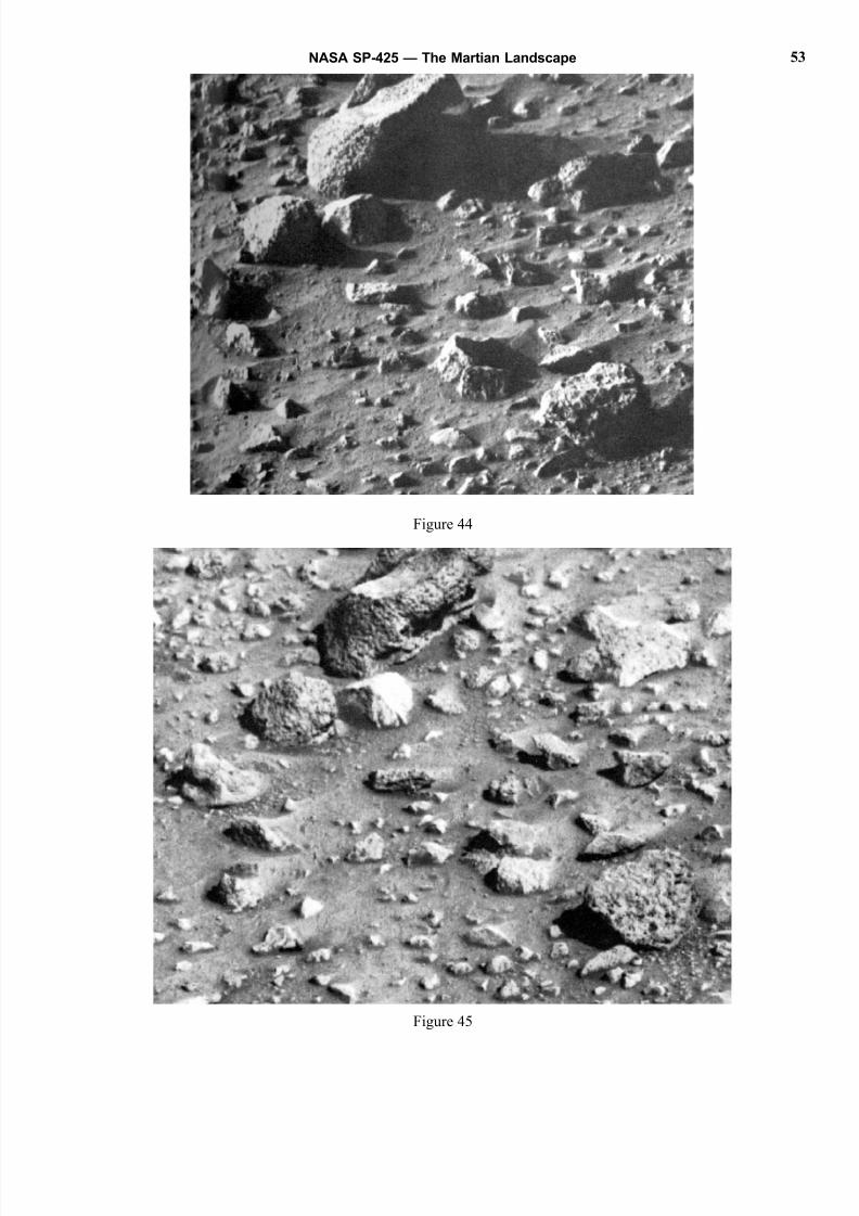
8/8/2019 The Martian Landscape
http://slidepdf.com/reader/full/the-martian-landscape 53/160
Figure 44
Figure 45
NASA SP-425 — The Martian Landscape 53
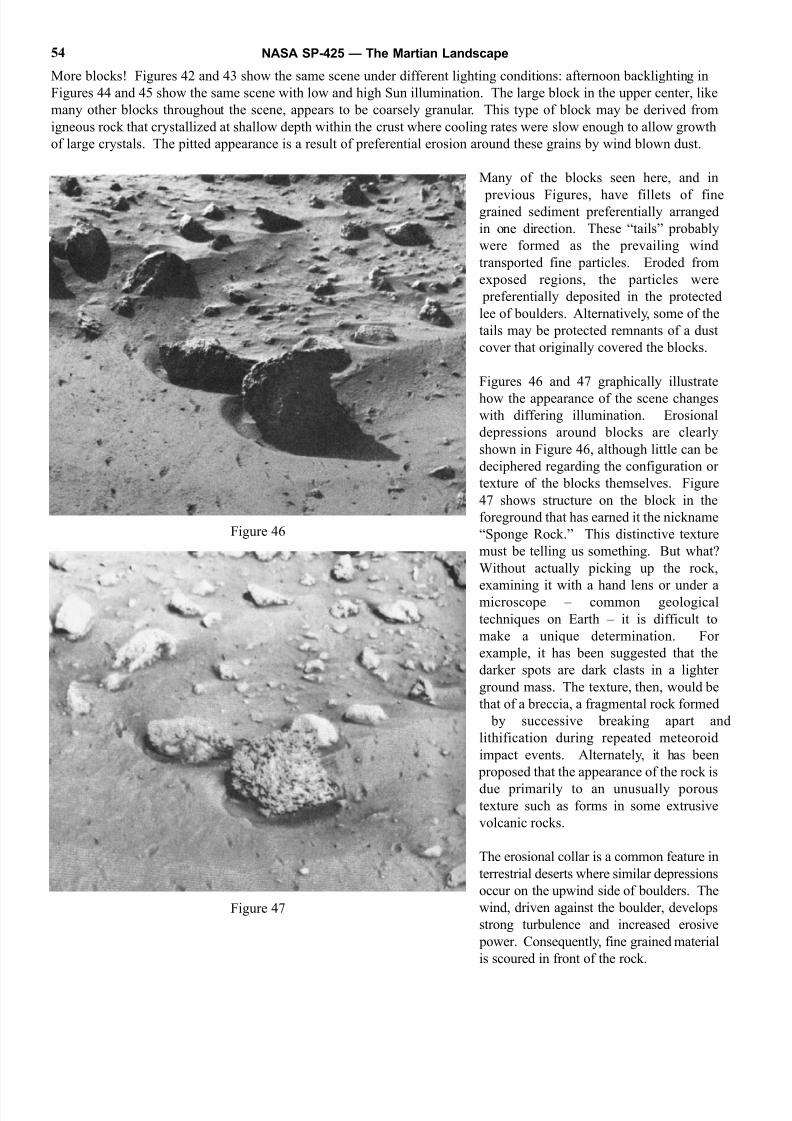
8/8/2019 The Martian Landscape
http://slidepdf.com/reader/full/the-martian-landscape 54/160
More blocks! Figures 42 and 43 show the same scene under different lighting conditions: afternoon backlighting in
Figures 44 and 45 show the same scene with low and high Sun illumination. The large block in the upper center, like
many other blocks throughout the scene, appears to be coarsely granular. This type of block may be derived from
igneous rock that crystallized at shallow depth within the crust where cooling rates were slow enough to allow growth
of large crystals. The pitted appearance is a result of preferential erosion around these grains by wind blown dust.
Many of the blocks seen here, and in
previous Figures, have fillets of finegrained sediment preferentially arranged
in one direction. These “tails” probably
were formed as the prevailing wind
transported fine particles. Eroded from
exposed regions, the particles were
preferentially deposited in the protected
lee of boulders. Alternatively, some of the
tails may be protected remnants of a dust
cover that originally covered the blocks.
Figures 46 and 47 graphically illustrate
how the appearance of the scene changes
with differing illumination. Erosional
depressions around blocks are clearly
shown in Figure 46, although little can be
deciphered regarding the configuration or
texture of the blocks themselves. Figure
47 shows structure on the block in the
foreground that has earned it the nickname
“Sponge Rock.” This distinctive texture
must be telling us something. But what?
Without actually picking up the rock,
examining it with a hand lens or under amicroscope – common geological
techniques on Earth – it is difficult to
make a unique determination. For
example, it has been suggested that the
darker spots are dark clasts in a lighter
ground mass. The texture, then, would be
that of a breccia, a fragmental rock formed
by successive breaking apart and
lithification during repeated meteoroid
impact events. Alternately, it has been
proposed that the appearance of the rock is
due primarily to an unusually poroustexture such as forms in some extrusive
volcanic rocks.
The erosional collar is a common feature in
terrestrial deserts where similar depressions
occur on the upwind side of boulders. The
wind, driven against the boulder, develops
strong turbulence and increased erosive
power. Consequently, fine grained material
is scoured in front of the rock.
NASA SP-425 — The Martian Landscape54
Figure 46
Figure 47
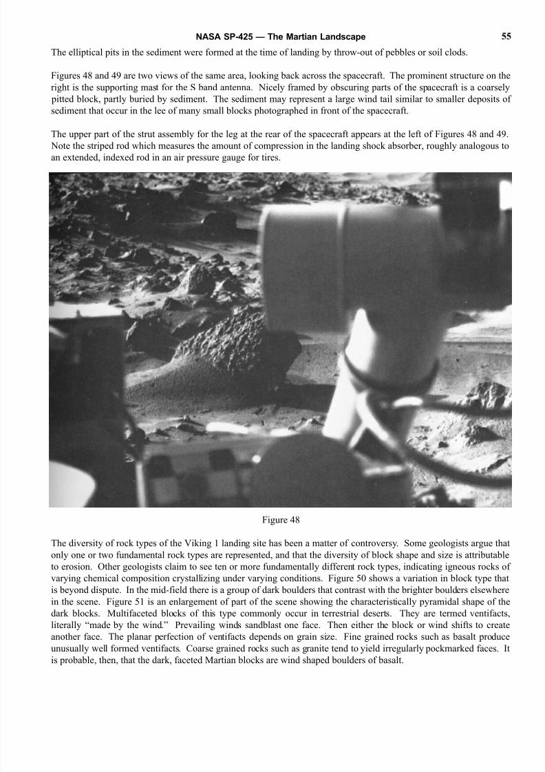
8/8/2019 The Martian Landscape
http://slidepdf.com/reader/full/the-martian-landscape 55/160
The elliptical pits in the sediment were formed at the time of landing by throw-out of pebbles or soil clods.
Figures 48 and 49 are two views of the same area, looking back across the spacecraft. The prominent structure on the
right is the supporting mast for the S band antenna. Nicely framed by obscuring parts of the spacecraft is a coarsely
pitted block, partly buried by sediment. The sediment may represent a large wind tail similar to smaller deposits o
sediment that occur in the lee of many small blocks photographed in front of the spacecraft.
The upper part of the strut assembly for the leg at the rear of the spacecraft appears at the left of Figures 48 and 49. Note the striped rod which measures the amount of compression in the landing shock absorber, roughly analogous to
an extended, indexed rod in an air pressure gauge for tires.
Figure 48
The diversity of rock types of the Viking 1 landing site has been a matter of controversy. Some geologists argue thatonly one or two fundamental rock types are represented, and that the diversity of block shape and size is attributable
to erosion. Other geologists claim to see ten or more fundamentally different rock types, indicating igneous rocks of
varying chemical composition crystallizing under varying conditions. Figure 50 shows a variation in block type that
is beyond dispute. In the mid-field there is a group of dark boulders that contrast with the brighter boulders elsewhere
in the scene. Figure 51 is an enlargement of part of the scene showing the characteristically pyramidal shape of the
dark blocks. Multifaceted blocks of this type commonly occur in terrestrial deserts. They are termed ventifacts
literally “made by the wind.” Prevailing winds sandblast one face. Then either the block or wind shifts to create
another face. The planar perfection of ventifacts depends on grain size. Fine grained rocks such as basalt produce
unusually well formed ventifacts. Coarse grained rocks such as granite tend to yield irregularly pockmarked faces. It
is probable, then, that the dark, faceted Martian blocks are wind shaped boulders of basalt.
NASA SP-425 — The Martian Landscape 55
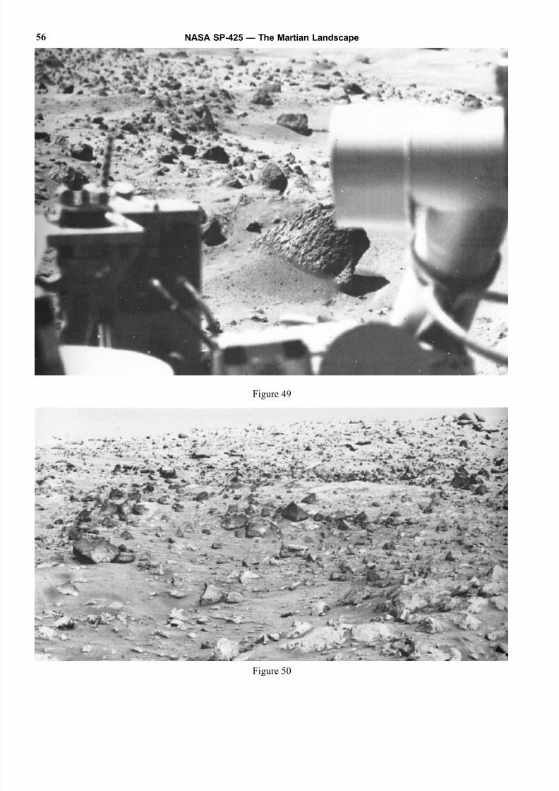
8/8/2019 The Martian Landscape
http://slidepdf.com/reader/full/the-martian-landscape 56/160
Figure 49
Figure 50
NASA SP-425 — The Martian Landscape56
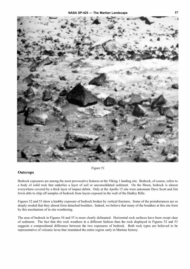
8/8/2019 The Martian Landscape
http://slidepdf.com/reader/full/the-martian-landscape 57/160
Figure 51
Outcrops
Bedrock exposures are among the most provocative features at the Viking 1 landing site. Bedrock, of course, refers to
a body of solid rock that underlies a layer of soil or unconsolidated sediment. On the Moon, bedrock is almost
everywhere covered by a thick layer of impact debris. Only at the Apollo 15 site were astronauts Dave Scott and JimIrwin able to chip off samples of bedrock from layers exposed in the wall of the Hadley Rille.
Figures 52 and 53 show a knobby exposure of bedrock broken by vertical fractures. Some of the protuberances are so
deeply eroded that they almost form detached boulders. Indeed, we believe that many of the boulders at this site form
by this mechanism of in situ weathering.
The area of bedrock in Figures 54 and 55 is more clearly delineated. Horizontal rock surfaces have been swept clear
of sediment. The fact that this rock weathers in a different fashion than the rock displayed in Figures 52 and 53
suggests a compositional difference between the two exposures of bedrock. Both rock types are believed to be
representative of volcanic lavas that inundated the entire region early in Martian history.
NASA SP-425 — The Martian Landscape 57
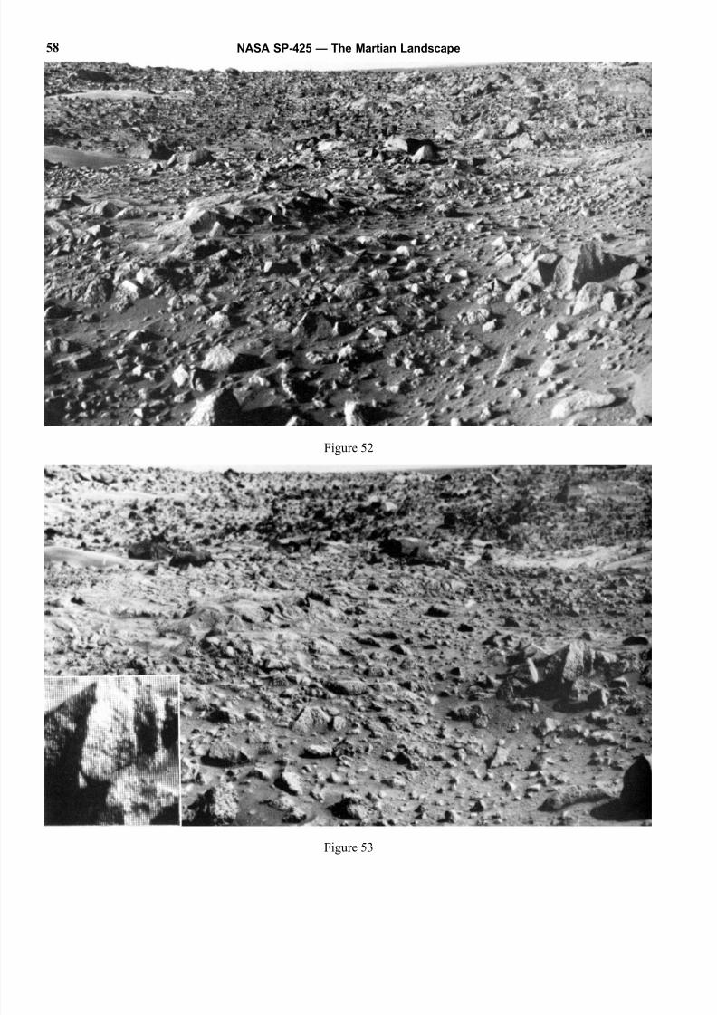
8/8/2019 The Martian Landscape
http://slidepdf.com/reader/full/the-martian-landscape 58/160
Figure 52
Figure 53
NASA SP-425 — The Martian Landscape58
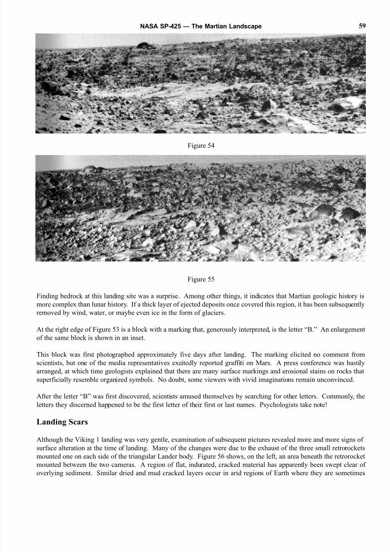
8/8/2019 The Martian Landscape
http://slidepdf.com/reader/full/the-martian-landscape 59/160
Figure 54
Figure 55
Finding bedrock at this landing site was a surprise. Among other things, it indicates that Martian geologic history is
more complex than lunar history. If a thick layer of ejected deposits once covered this region, it has been subsequently
removed by wind, water, or maybe even ice in the form of glaciers.
At the right edge of Figure 53 is a block with a marking that, generously interpreted, is the letter “B.” An enlargement
of the same block is shown in an inset.
This block was first photographed approximately five days after landing. The marking elicited no comment from
scientists, but one of the media representatives excitedly reported graffiti on Mars. A press conference was hastily
arranged, at which time geologists explained that there are many surface markings and erosional stains on rocks that
superficially resemble organized symbols. No doubt, some viewers with vivid imaginations remain unconvinced.
After the letter “B” was first discovered, scientists amused themselves by searching for other letters. Commonly, the
letters they discerned happened to be the first letter of their first or last names. Psychologists take note!
Landing Scars
Although the Viking 1 landing was very gentle, examination of subsequent pictures revealed more and more signs of
surface alteration at the time of landing. Many of the changes were due to the exhaust of the three small retrorockets
mounted one on each side of the triangular Lander body. Figure 56 shows, on the left, an area beneath the retrorocket
mounted between the two cameras. A region of flat, indurated, cracked material has apparently been swept clear of
overlying sediment. Similar dried and mud cracked layers occur in arid regions of Earth where they are sometimes
NASA SP-425 — The Martian Landscape 59
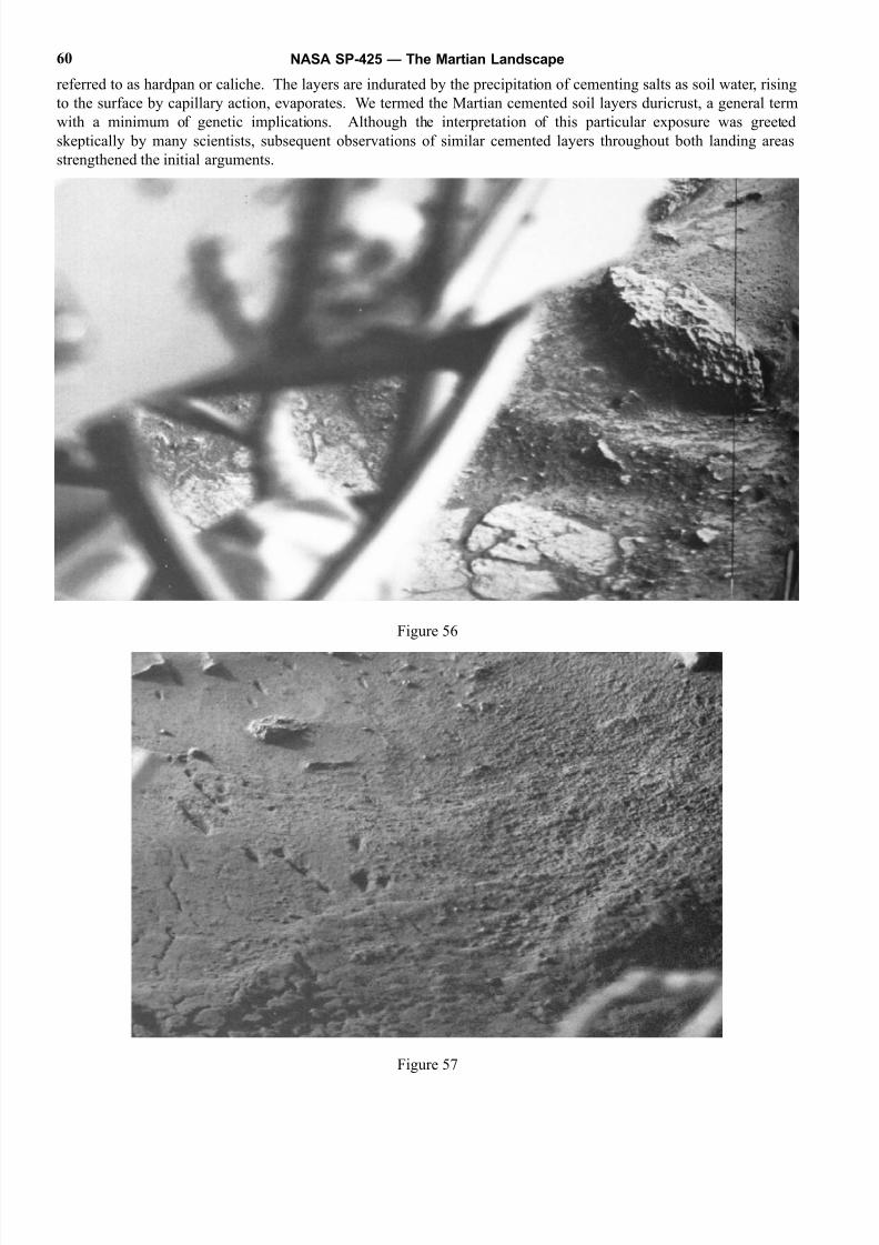
8/8/2019 The Martian Landscape
http://slidepdf.com/reader/full/the-martian-landscape 60/160
referred to as hardpan or caliche. The layers are indurated by the precipitation of cementing salts as soil water, rising
to the surface by capillary action, evaporates. We termed the Martian cemented soil layers duricrust, a general term
with a minimum of genetic implications. Although the interpretation of this particular exposure was greeted
skeptically by many scientists, subsequent observations of similar cemented layers throughout both landing areas
strengthened the initial arguments.
Figure 56
Figure 57
NASA SP-425 — The Martian Landscape60
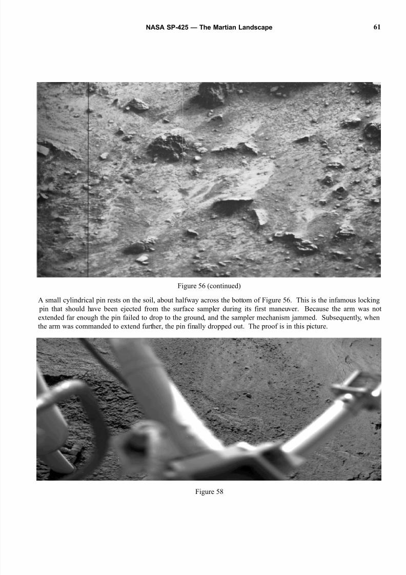
8/8/2019 The Martian Landscape
http://slidepdf.com/reader/full/the-martian-landscape 61/160
A small cylindrical pin rests on the soil, about halfway across the bottom of Figure 56. This is the infamous locking pin that should have been ejected from the surface sampler during its first maneuver. Because the arm was no
extended far enough the pin failed to drop to the ground, and the sampler mechanism jammed. Subsequently, when
the arm was commanded to extend further, the pin finally dropped out. The proof is in this picture.
Figure 58
NASA SP-425 — The Martian Landscape 61
Figure 56 (continued)
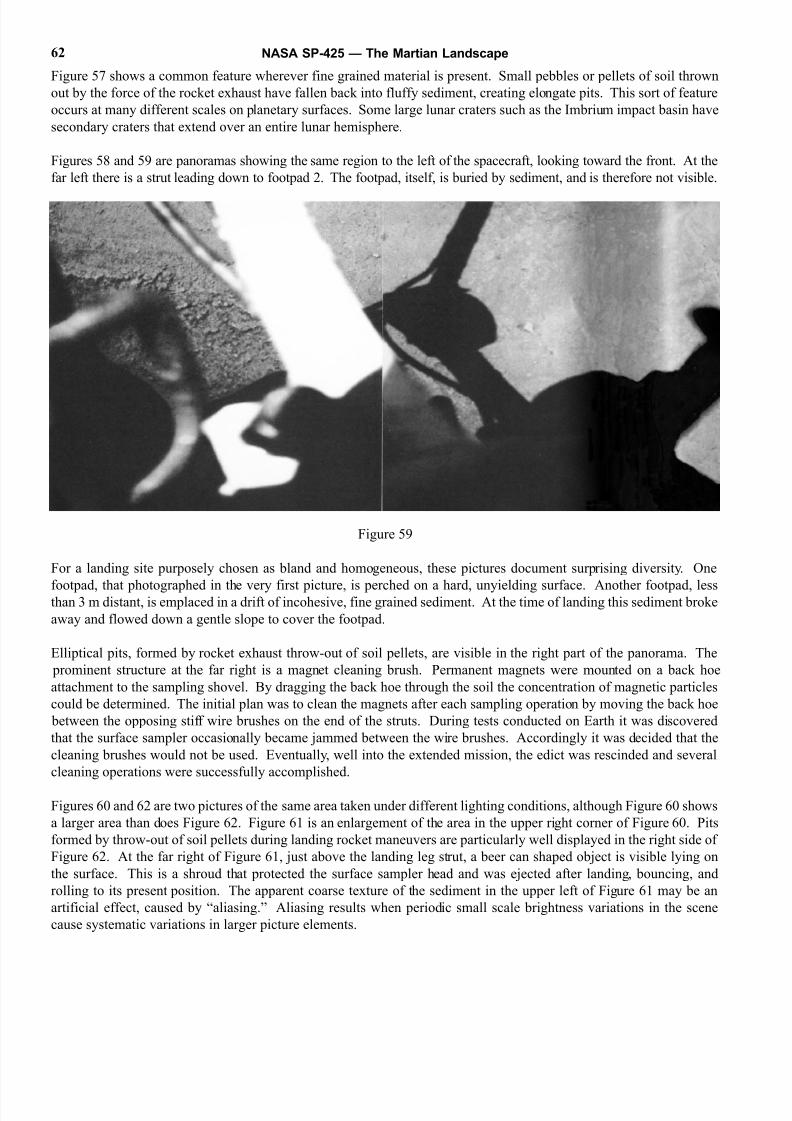
8/8/2019 The Martian Landscape
http://slidepdf.com/reader/full/the-martian-landscape 62/160
Figure 57 shows a common feature wherever fine grained material is present. Small pebbles or pellets of soil thrown
out by the force of the rocket exhaust have fallen back into fluffy sediment, creating elongate pits. This sort of feature
occurs at many different scales on planetary surfaces. Some large lunar craters such as the Imbrium impact basin have
secondary craters that extend over an entire lunar hemisphere.
Figures 58 and 59 are panoramas showing the same region to the left of the spacecraft, looking toward the front. At the
far left there is a strut leading down to footpad 2. The footpad, itself, is buried by sediment, and is therefore not visible.
Figure 59
For a landing site purposely chosen as bland and homogeneous, these pictures document surprising diversity. One
footpad, that photographed in the very first picture, is perched on a hard, unyielding surface. Another footpad, lessthan 3 m distant, is emplaced in a drift of incohesive, fine grained sediment. At the time of landing this sediment broke
away and flowed down a gentle slope to cover the footpad.
Elliptical pits, formed by rocket exhaust throw-out of soil pellets, are visible in the right part of the panorama. The
prominent structure at the far right is a magnet cleaning brush. Permanent magnets were mounted on a back hoe
attachment to the sampling shovel. By dragging the back hoe through the soil the concentration of magnetic particles
could be determined. The initial plan was to clean the magnets after each sampling operation by moving the back hoe
between the opposing stiff wire brushes on the end of the struts. During tests conducted on Earth it was discovered
that the surface sampler occasionally became jammed between the wire brushes. Accordingly it was decided that the
cleaning brushes would not be used. Eventually, well into the extended mission, the edict was rescinded and several
cleaning operations were successfully accomplished.
Figures 60 and 62 are two pictures of the same area taken under different lighting conditions, although Figure 60 shows
a larger area than does Figure 62. Figure 61 is an enlargement of the area in the upper right corner of Figure 60. Pits
formed by throw-out of soil pellets during landing rocket maneuvers are particularly well displayed in the right side of
Figure 62. At the far right of Figure 61, just above the landing leg strut, a beer can shaped object is visible lying on
the surface. This is a shroud that protected the surface sampler head and was ejected after landing, bouncing, and
rolling to its present position. The apparent coarse texture of the sediment in the upper left of Figure 61 may be an
artificial effect, caused by “aliasing.” Aliasing results when periodic small scale brightness variations in the scene
cause systematic variations in larger picture elements.
NASA SP-425 — The Martian Landscape62
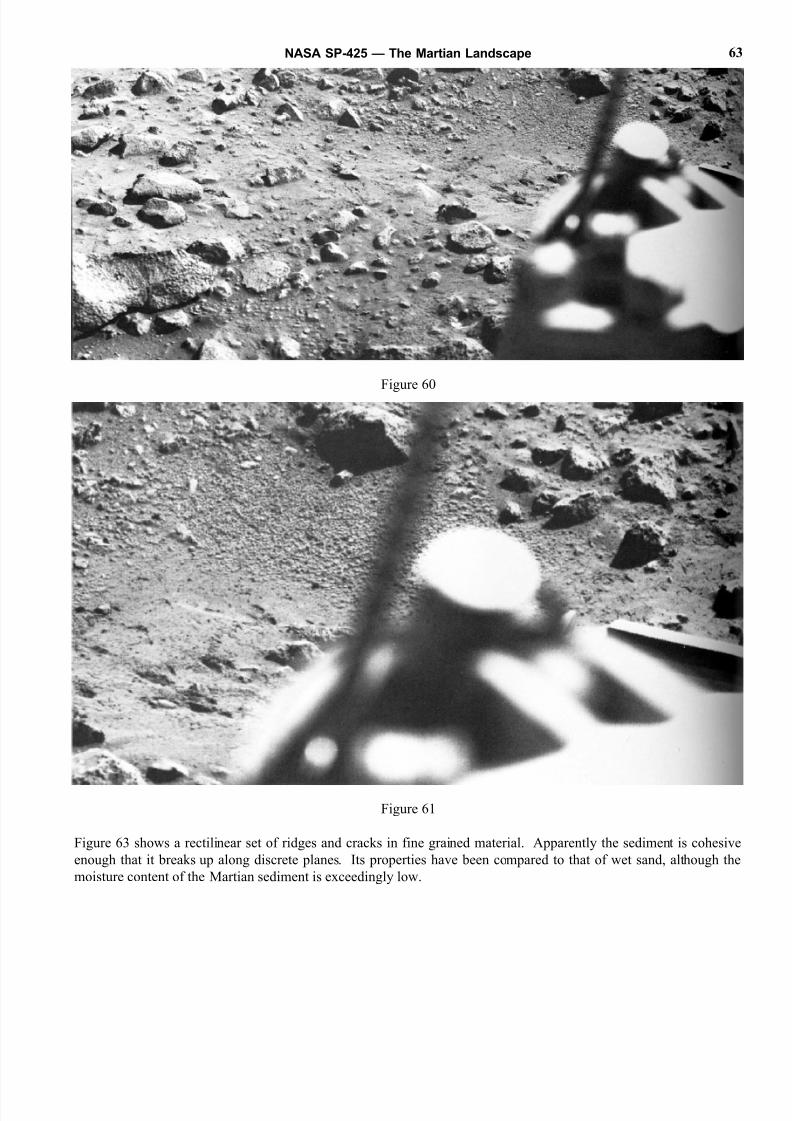
8/8/2019 The Martian Landscape
http://slidepdf.com/reader/full/the-martian-landscape 63/160
Figure 60
Figure 61
Figure 63 shows a rectilinear set of ridges and cracks in fine grained material. Apparently the sediment is cohesive
enough that it breaks up along discrete planes. Its properties have been compared to that of wet sand, although the
moisture content of the Martian sediment is exceedingly low.
NASA SP-425 — The Martian Landscape 63
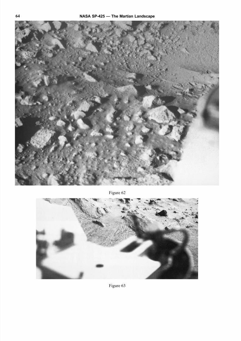
8/8/2019 The Martian Landscape
http://slidepdf.com/reader/full/the-martian-landscape 64/160
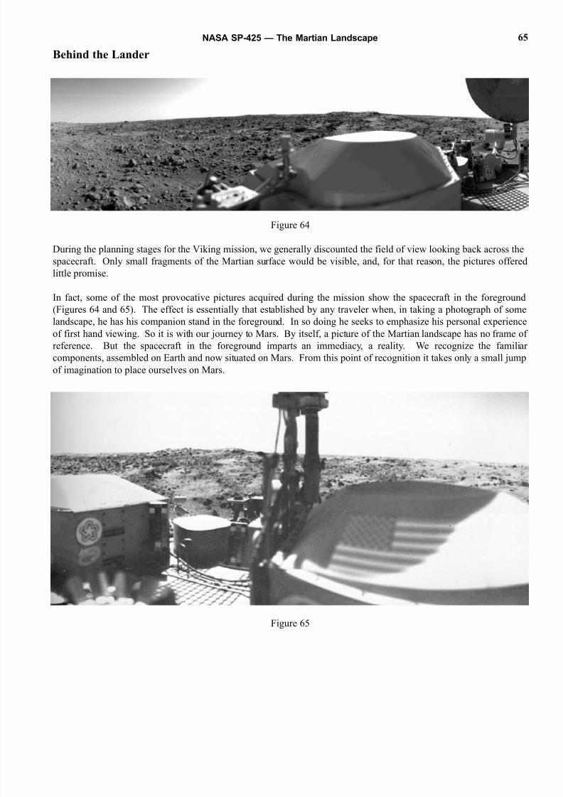
8/8/2019 The Martian Landscape
http://slidepdf.com/reader/full/the-martian-landscape 65/160
Behind the Lander
Figure 64
During the planning stages for the Viking mission, we generally discounted the field of view looking back across the
spacecraft. Only small fragments of the Martian surface would be visible, and, for that reason, the pictures offered
little promise.
In fact, some of the most provocative pictures acquired during the mission show the spacecraft in the foreground
(Figures 64 and 65). The effect is essentially that established by any traveler when, in taking a photograph of some
landscape, he has his companion stand in the foreground. In so doing he seeks to emphasize his personal experience
of first hand viewing. So it is with our journey to Mars. By itself, a picture of the Martian landscape has no frame of
reference. But the spacecraft in the foreground imparts an immediacy, a reality. We recognize the familiar
components, assembled on Earth and now situated on Mars. From this point of recognition it takes only a small jump
of imagination to place ourselves on Mars.
Figure 65
NASA SP-425 — The Martian Landscape 65
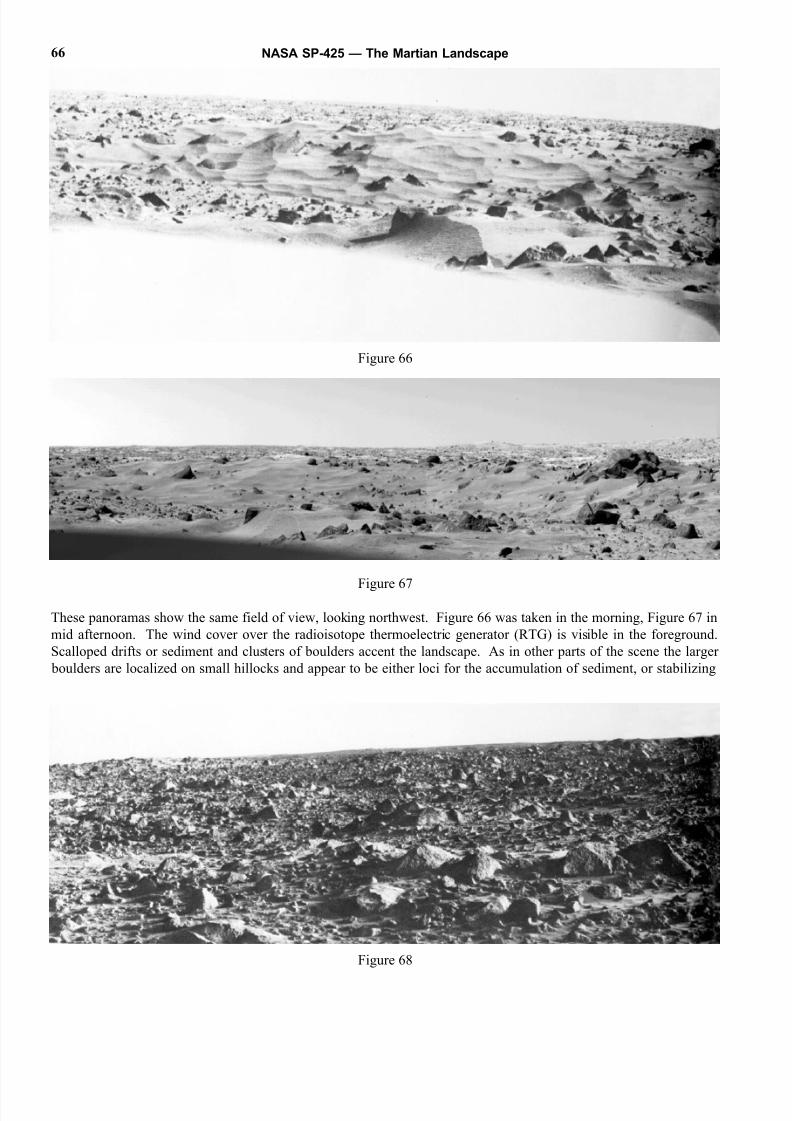
8/8/2019 The Martian Landscape
http://slidepdf.com/reader/full/the-martian-landscape 66/160
Figure 67
These panoramas show the same field of view, looking northwest. Figure 66 was taken in the morning, Figure 67 in
mid afternoon. The wind cover over the radioisotope thermoelectric generator (RTG) is visible in the foreground.
Scalloped drifts or sediment and clusters of boulders accent the landscape. As in other parts of the scene the larger
boulders are localized on small hillocks and appear to be either loci for the accumulation of sediment, or stabilizing
NASA SP-425 — The Martian Landscape66
Figure 66
Figure 68
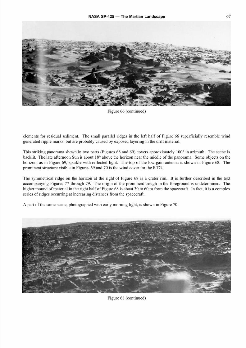
8/8/2019 The Martian Landscape
http://slidepdf.com/reader/full/the-martian-landscape 67/160
elements for residual sediment. The small parallel ridges in the left half of Figure 66 superficially resemble wind
generated ripple marks, but are probably caused by exposed layering in the drift material.
This striking panorama shown in two parts (Figures 68 and 69) covers approximately 100° in azimuth. The scene is
backlit. The late afternoon Sun is about 18° above the horizon near the middle of the panorama. Some objects on the
horizon, as in Figure 69, sparkle with reflected light. The top of the low gain antenna is shown in Figure 68. The
prominent structure visible in Figures 69 and 70 is the wind cover for the RTG.
The symmetrical ridge on the horizon at the right of Figure 68 is a crater rim. It is further described in the text
accompanying Figures 77 through 79. The origin of the prominent trough in the foreground is undetermined. Thehigher mound of material in the right half of Figure 68 is about 30 to 60 m from the spacecraft. In fact, it is a complex
series of ridges occurring at increasing distances from the spacecraft.
A part of the same scene, photographed with early morning light, is shown in Figure 70.
NASA SP-425 — The Martian Landscape 67
Figure 66 (continued)
Figure 68 (continued)
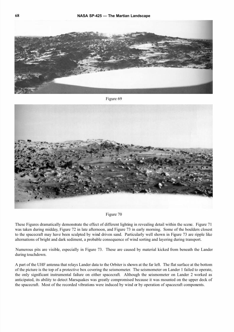
8/8/2019 The Martian Landscape
http://slidepdf.com/reader/full/the-martian-landscape 68/160
Figure 69
Figure 70
These Figures dramatically demonstrate the effect of different lighting in revealing detail within the scene. Figure 71
was taken during midday, Figure 72 in late afternoon, and Figure 73 in early morning. Some of the boulders closest
to the spacecraft may have been sculpted by wind driven sand. Particularly well shown in Figure 73 are ripple like
alternations of bright and dark sediment, a probable consequence of wind sorting and layering during transport.
Numerous pits are visible, especially in Figure 73. These are caused by material kicked from beneath the Lander
during touchdown.
A part of the UHF antenna that relays Lander data to the Orbiter is shown at the far left. The flat surface at the bottom
of the picture is the top of a protective box covering the seismometer. The seismometer on Lander 1 failed to operate,
the only significant instrumental failure on either spacecraft. Although the seismometer on Lander 2 worked as
anticipated, its ability to detect Marsquakes was greatly compromised because it was mounted on the upper deck of
the spacecraft. Most of the recorded vibrations were induced by wind or by operation of spacecraft components.
NASA SP-425 — The Martian Landscape68
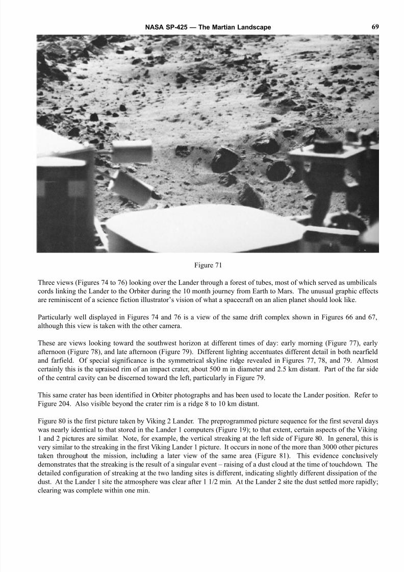
8/8/2019 The Martian Landscape
http://slidepdf.com/reader/full/the-martian-landscape 69/160
Figure 71
Three views (Figures 74 to 76) looking over the Lander through a forest of tubes, most of which served as umbilicals
cords linking the Lander to the Orbiter during the 10 month journey from Earth to Mars. The unusual graphic effects
are reminiscent of a science fiction illustrator’s vision of what a spacecraft on an alien planet should look like.
Particularly well displayed in Figures 74 and 76 is a view of the same drift complex shown in Figures 66 and 67,
although this view is taken with the other camera.
These are views looking toward the southwest horizon at different times of day: early morning (Figure 77), early
afternoon (Figure 78), and late afternoon (Figure 79). Different lighting accentuates different detail in both nearfield
and farfield. Of special significance is the symmetrical skyline ridge revealed in Figures 77, 78, and 79. Almost
certainly this is the upraised rim of an impact crater, about 500 m in diameter and 2.5 km distant. Part of the far side
of the central cavity can be discerned toward the left, particularly in Figure 79.
This same crater has been identified in Orbiter photographs and has been used to locate the Lander position. Refer to
Figure 204. Also visible beyond the crater rim is a ridge 8 to 10 km distant.
Figure 80 is the first picture taken by Viking 2 Lander. The preprogrammed picture sequence for the first several days
was nearly identical to that stored in the Lander 1 computers (Figure 19); to that extent, certain aspects of the Viking
1 and 2 pictures are similar. Note, for example, the vertical streaking at the left side of Figure 80. In general, this is
very similar to the streaking in the first Viking Lander 1 picture. It occurs in none of the more than 3000 other pictures
taken throughout the mission, including a later view of the same area (Figure 81). This evidence conclusively
demonstrates that the streaking is the result of a singular event – raising of a dust cloud at the time of touchdown. The
detailed configuration of streaking at the two landing sites is different, indicating slightly different dissipation of the
dust. At the Lander 1 site the atmosphere was clear after 1 1/2 min. At the Lander 2 site the dust settled more rapidly
clearing was complete within one min.
NASA SP-425 — The Martian Landscape 69
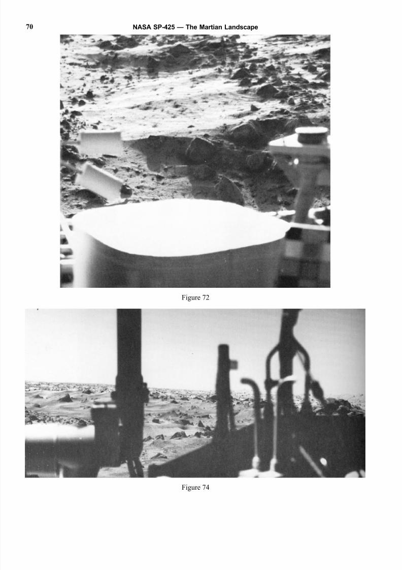
8/8/2019 The Martian Landscape
http://slidepdf.com/reader/full/the-martian-landscape 70/160
Figure 72
Figure 74
NASA SP-425 — The Martian Landscape70
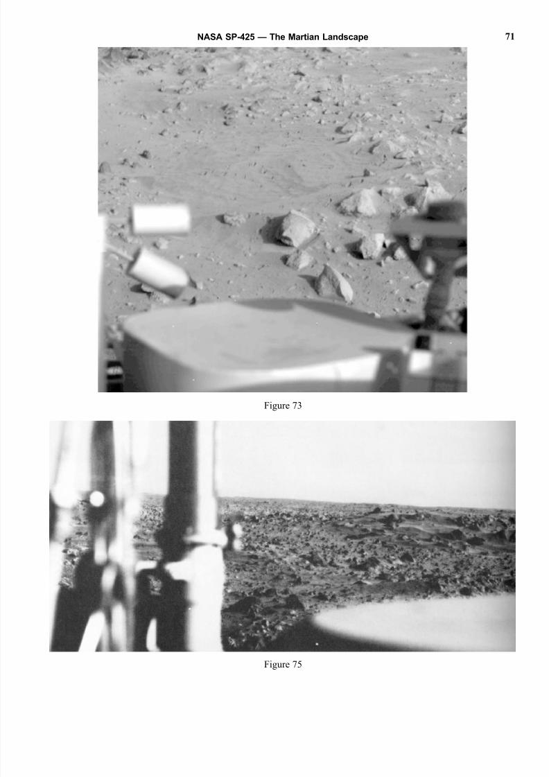
8/8/2019 The Martian Landscape
http://slidepdf.com/reader/full/the-martian-landscape 71/160
Figure 73
Figure 75
NASA SP-425 — The Martian Landscape 71
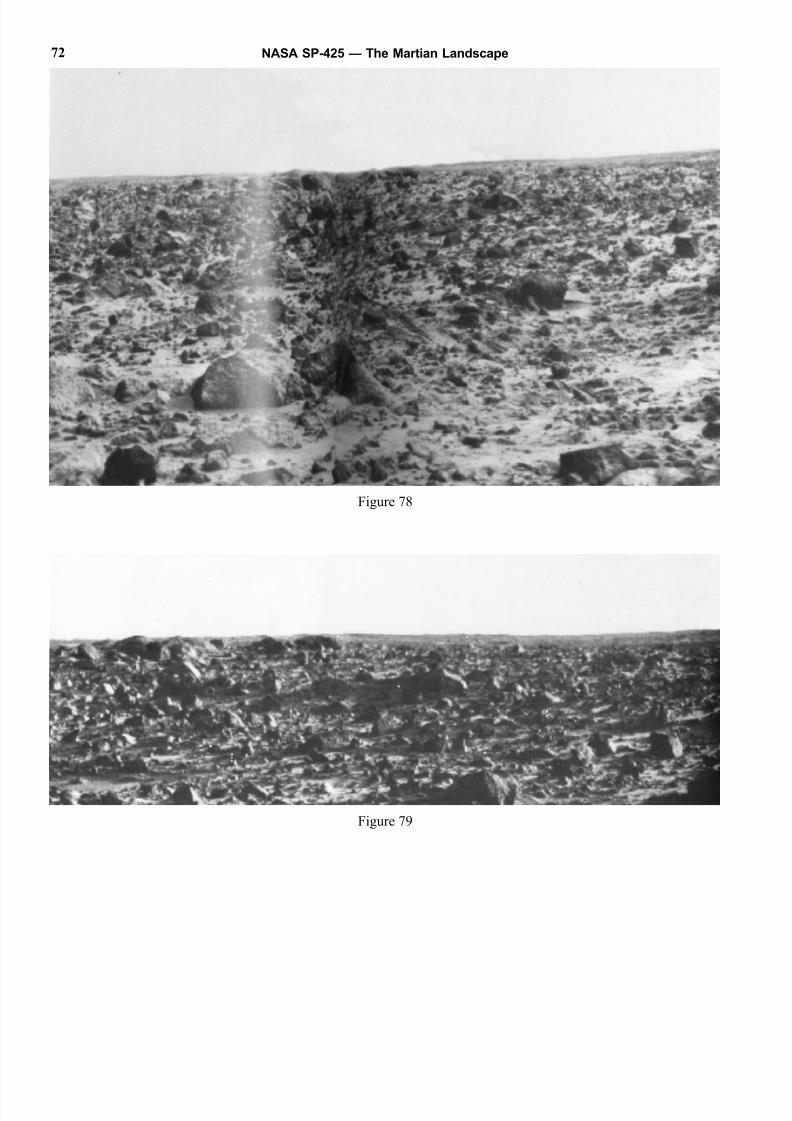
8/8/2019 The Martian Landscape
http://slidepdf.com/reader/full/the-martian-landscape 72/160
NASA SP-425 — The Martian Landscape72
Figure 79
Figure 78
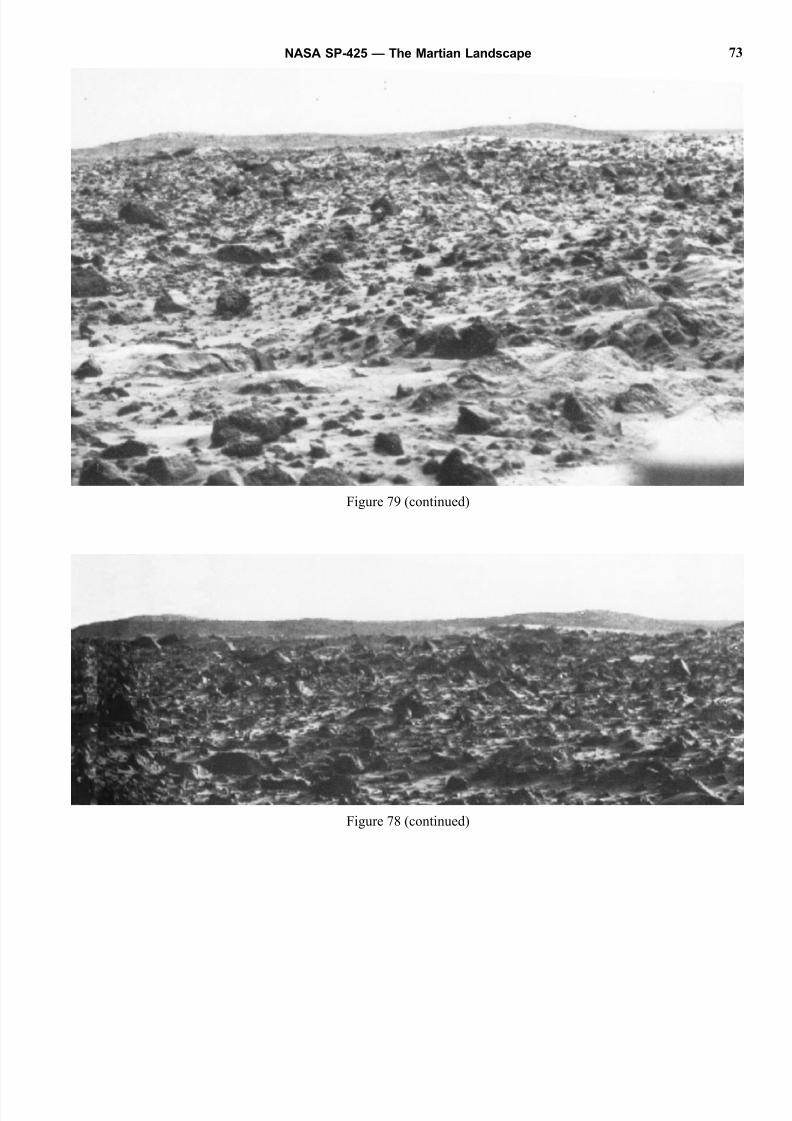
8/8/2019 The Martian Landscape
http://slidepdf.com/reader/full/the-martian-landscape 73/160
NASA SP-425 — The Martian Landscape 73
Figure 78 (continued)
Figure 79 (continued)
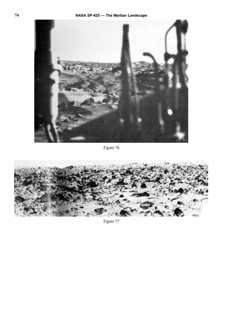
8/8/2019 The Martian Landscape
http://slidepdf.com/reader/full/the-martian-landscape 74/160
NASA SP-425 — The Martian Landscape74
Figure 76
Figure 77
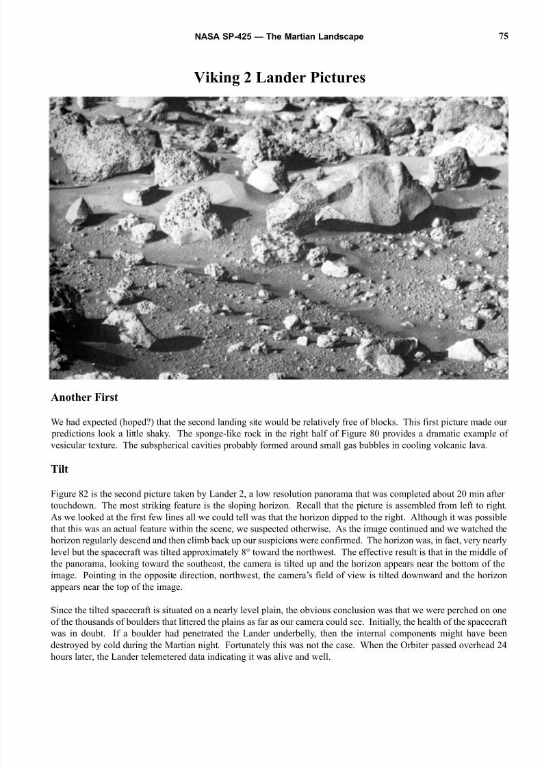
8/8/2019 The Martian Landscape
http://slidepdf.com/reader/full/the-martian-landscape 75/160
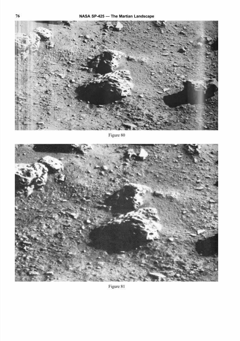
8/8/2019 The Martian Landscape
http://slidepdf.com/reader/full/the-martian-landscape 76/160
NASA SP-425 — The Martian Landscape76
Figure 80
Figure 81
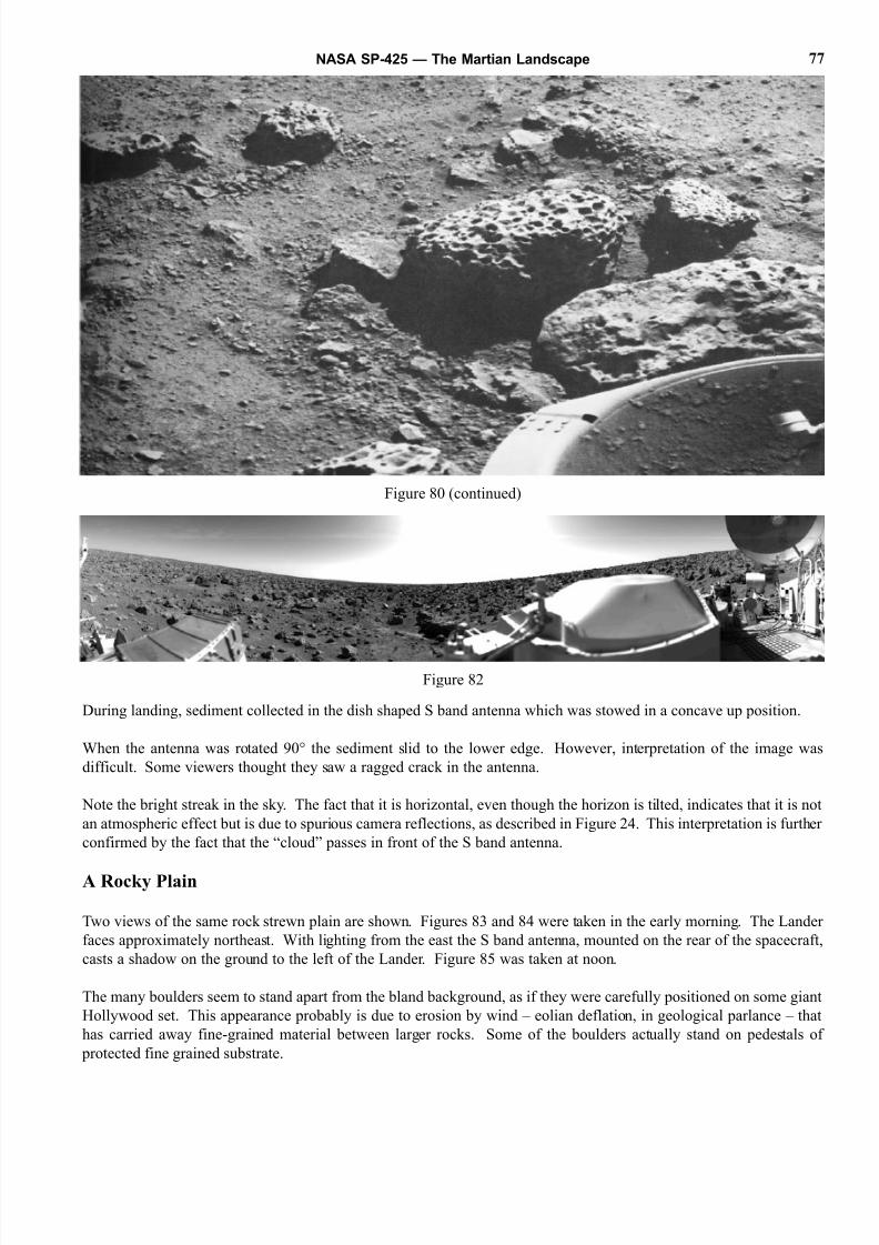
8/8/2019 The Martian Landscape
http://slidepdf.com/reader/full/the-martian-landscape 77/160
During landing, sediment collected in the dish shaped S band antenna which was stowed in a concave up position.
When the antenna was rotated 90° the sediment slid to the lower edge. However, interpretation of the image was
difficult. Some viewers thought they saw a ragged crack in the antenna.
Note the bright streak in the sky. The fact that it is horizontal, even though the horizon is tilted, indicates that it is not
an atmospheric effect but is due to spurious camera reflections, as described in Figure 24. This interpretation is further
confirmed by the fact that the “cloud” passes in front of the S band antenna.
A Rocky Plain
Two views of the same rock strewn plain are shown. Figures 83 and 84 were taken in the early morning. The Lander
faces approximately northeast. With lighting from the east the S band antenna, mounted on the rear of the spacecraft
casts a shadow on the ground to the left of the Lander. Figure 85 was taken at noon.
The many boulders seem to stand apart from the bland background, as if they were carefully positioned on some giant
Hollywood set. This appearance probably is due to erosion by wind – eolian deflation, in geological parlance – that
has carried away fine-grained material between larger rocks. Some of the boulders actually stand on pedestals of
protected fine grained substrate.
NASA SP-425 — The Martian Landscape 77
Figure 82
Figure 80 (continued)
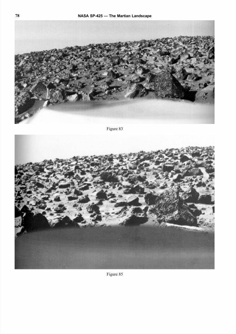
8/8/2019 The Martian Landscape
http://slidepdf.com/reader/full/the-martian-landscape 78/160
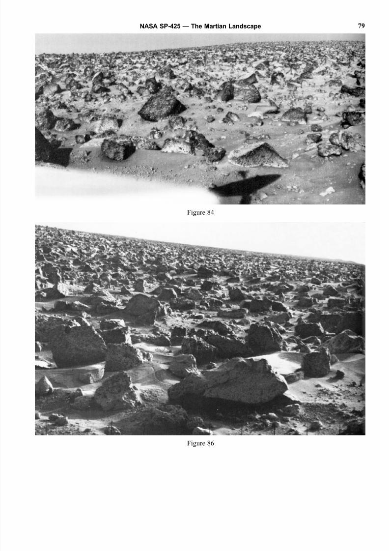
8/8/2019 The Martian Landscape
http://slidepdf.com/reader/full/the-martian-landscape 79/160
NASA SP-425 — The Martian Landscape 79
Figure 86
Figure 84
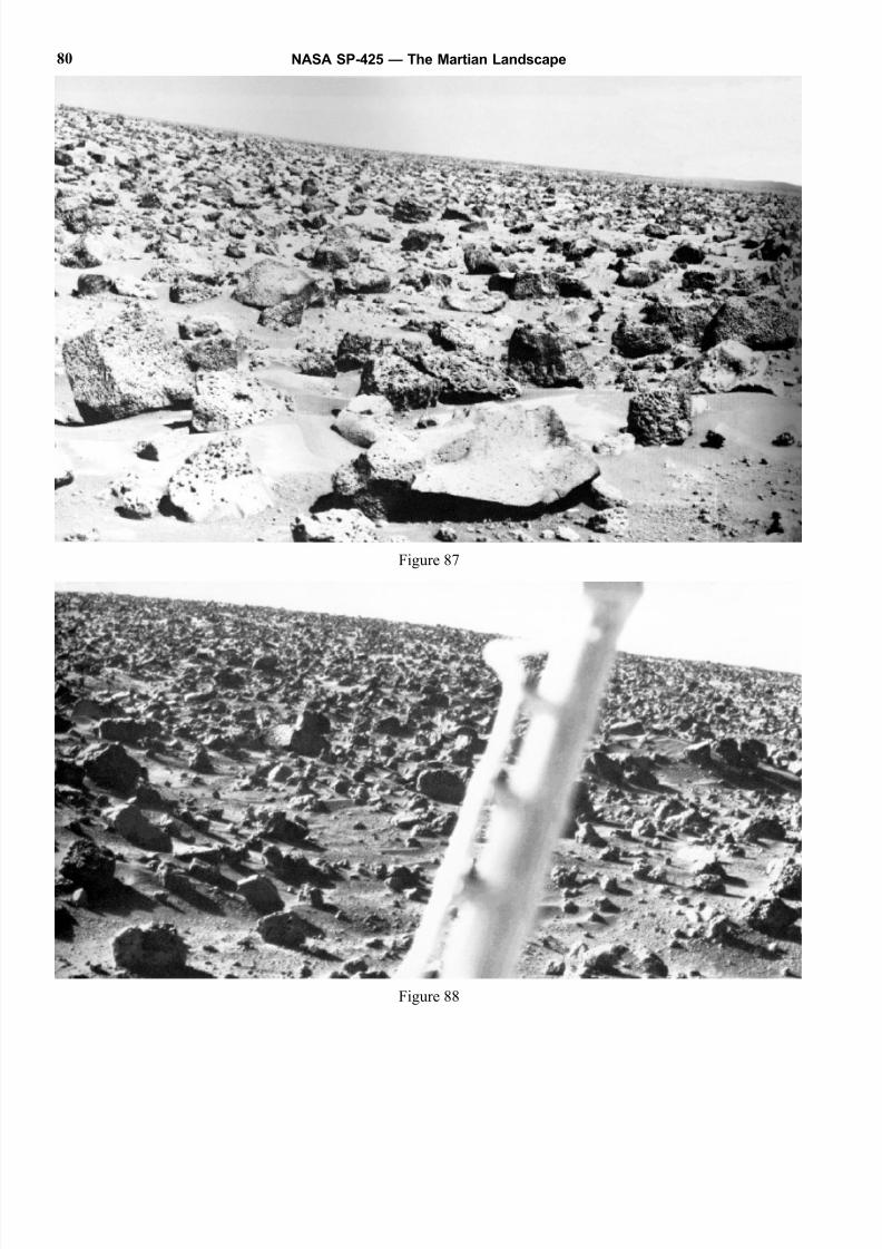
8/8/2019 The Martian Landscape
http://slidepdf.com/reader/full/the-martian-landscape 80/160
NASA SP-425 — The Martian Landscape80
Figure 87
Figure 88
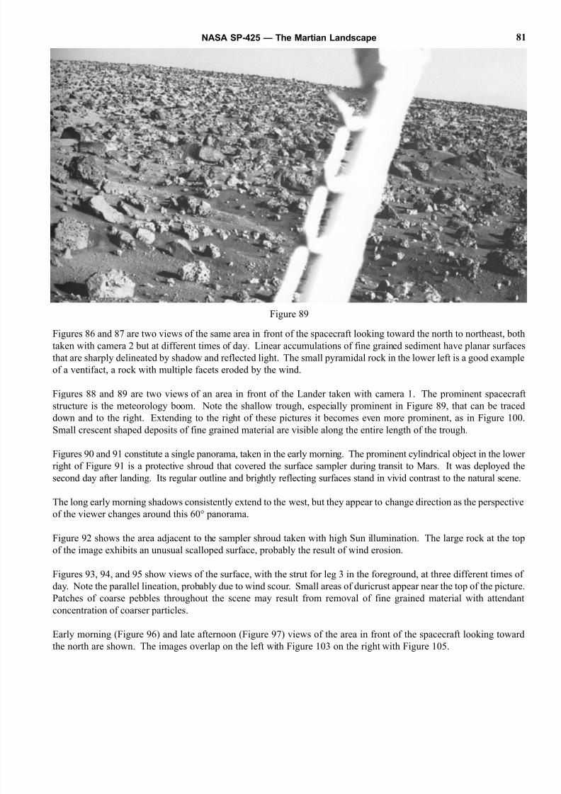
8/8/2019 The Martian Landscape
http://slidepdf.com/reader/full/the-martian-landscape 81/160
Figures 86 and 87 are two views of the same area in front of the spacecraft looking toward the north to northeast, both
taken with camera 2 but at different times of day. Linear accumulations of fine grained sediment have planar surfaces
that are sharply delineated by shadow and reflected light. The small pyramidal rock in the lower left is a good example
of a ventifact, a rock with multiple facets eroded by the wind.
Figures 88 and 89 are two views of an area in front of the Lander taken with camera 1. The prominent spacecraft
structure is the meteorology boom. Note the shallow trough, especially prominent in Figure 89, that can be traced
down and to the right. Extending to the right of these pictures it becomes even more prominent, as in Figure 100Small crescent shaped deposits of fine grained material are visible along the entire length of the trough.
Figures 90 and 91 constitute a single panorama, taken in the early morning. The prominent cylindrical object in the lower
right of Figure 91 is a protective shroud that covered the surface sampler during transit to Mars. It was deployed the
second day after landing. Its regular outline and brightly reflecting surfaces stand in vivid contrast to the natural scene.
The long early morning shadows consistently extend to the west, but they appear to change direction as the perspective
of the viewer changes around this 60° panorama.
Figure 92 shows the area adjacent to the sampler shroud taken with high Sun illumination. The large rock at the top
of the image exhibits an unusual scalloped surface, probably the result of wind erosion.
Figures 93, 94, and 95 show views of the surface, with the strut for leg 3 in the foreground, at three different times of
day. Note the parallel lineation, probably due to wind scour. Small areas of duricrust appear near the top of the picture
Patches of coarse pebbles throughout the scene may result from removal of fine grained material with attendant
concentration of coarser particles.
Early morning (Figure 96) and late afternoon (Figure 97) views of the area in front of the spacecraft looking toward
the north are shown. The images overlap on the left with Figure 103 on the right with Figure 105.
NASA SP-425 — The Martian Landscape 81
Figure 89
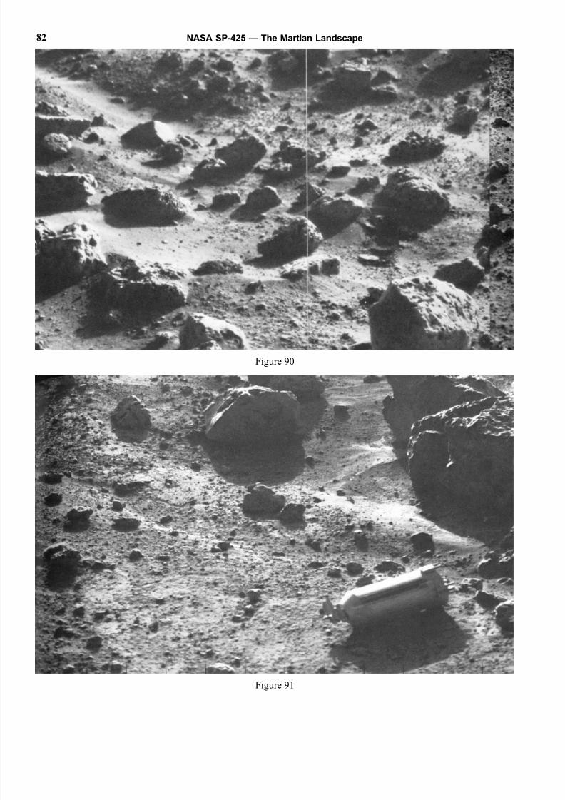
8/8/2019 The Martian Landscape
http://slidepdf.com/reader/full/the-martian-landscape 82/160
NASA SP-425 — The Martian Landscape82
Figure 90
Figure 91
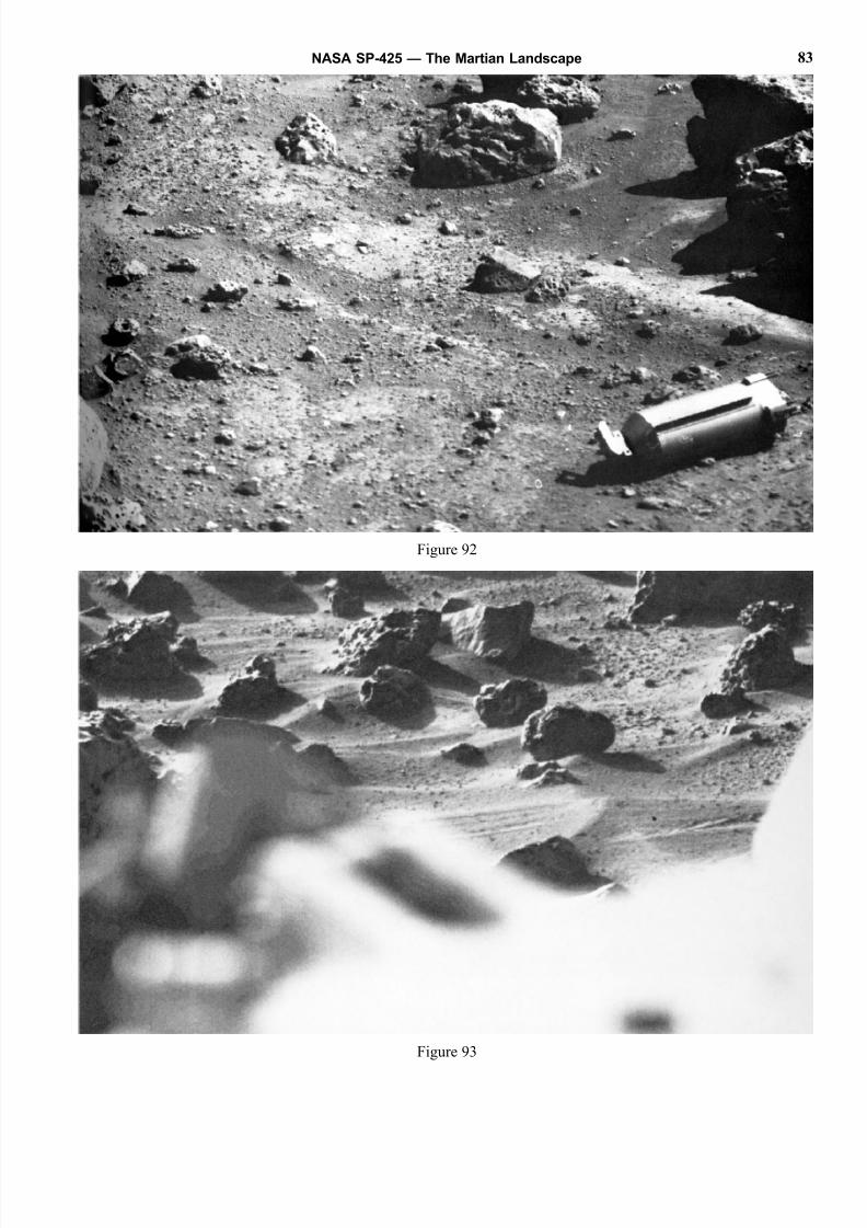
8/8/2019 The Martian Landscape
http://slidepdf.com/reader/full/the-martian-landscape 83/160
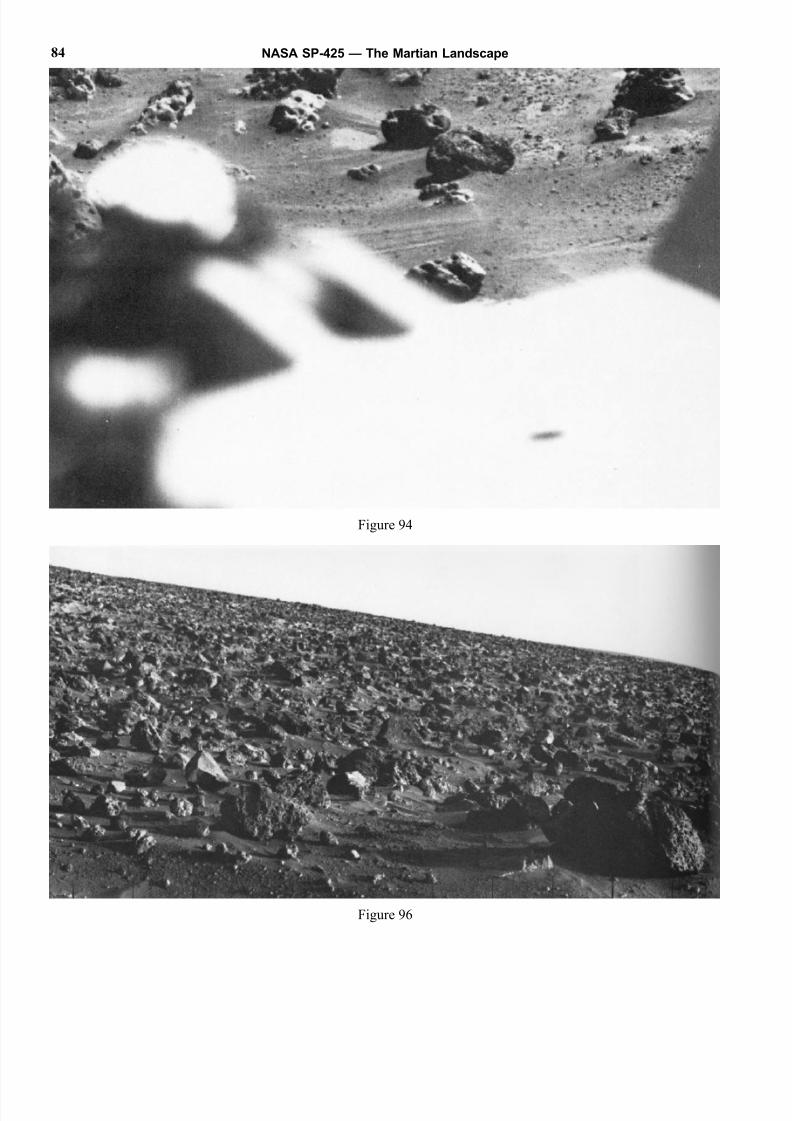
8/8/2019 The Martian Landscape
http://slidepdf.com/reader/full/the-martian-landscape 84/160
NASA SP-425 — The Martian Landscape84
Figure 94
Figure 96
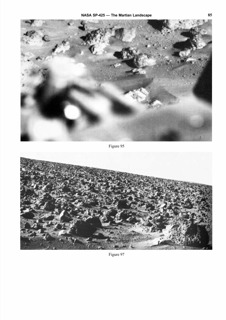
8/8/2019 The Martian Landscape
http://slidepdf.com/reader/full/the-martian-landscape 85/160
NASA SP-425 — The Martian Landscape 85
Figure 97
Figure 95
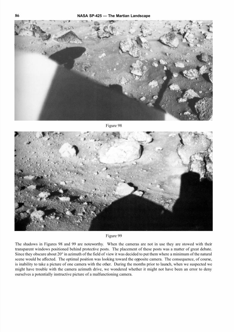
8/8/2019 The Martian Landscape
http://slidepdf.com/reader/full/the-martian-landscape 86/160
The shadows in Figures 98 and 99 are noteworthy. When the cameras are not in use they are stowed with their
transparent windows positioned behind protective posts. The placement of these posts was a matter of great debate.
Since they obscure about 20° in azimuth of the field of view it was decided to put them where a minimum of the natural
scene would be affected. The optimal position was looking toward the opposite camera. The consequence, of course,
is inability to take a picture of one camera with the other. During the months prior to launch, when we suspected we
might have trouble with the camera azimuth drive, we wondered whether it might not have been an error to deny
ourselves a potentially instructive picture of a malfunctioning camera.
NASA SP-425 — The Martian Landscape86
Figure 98
Figure 99
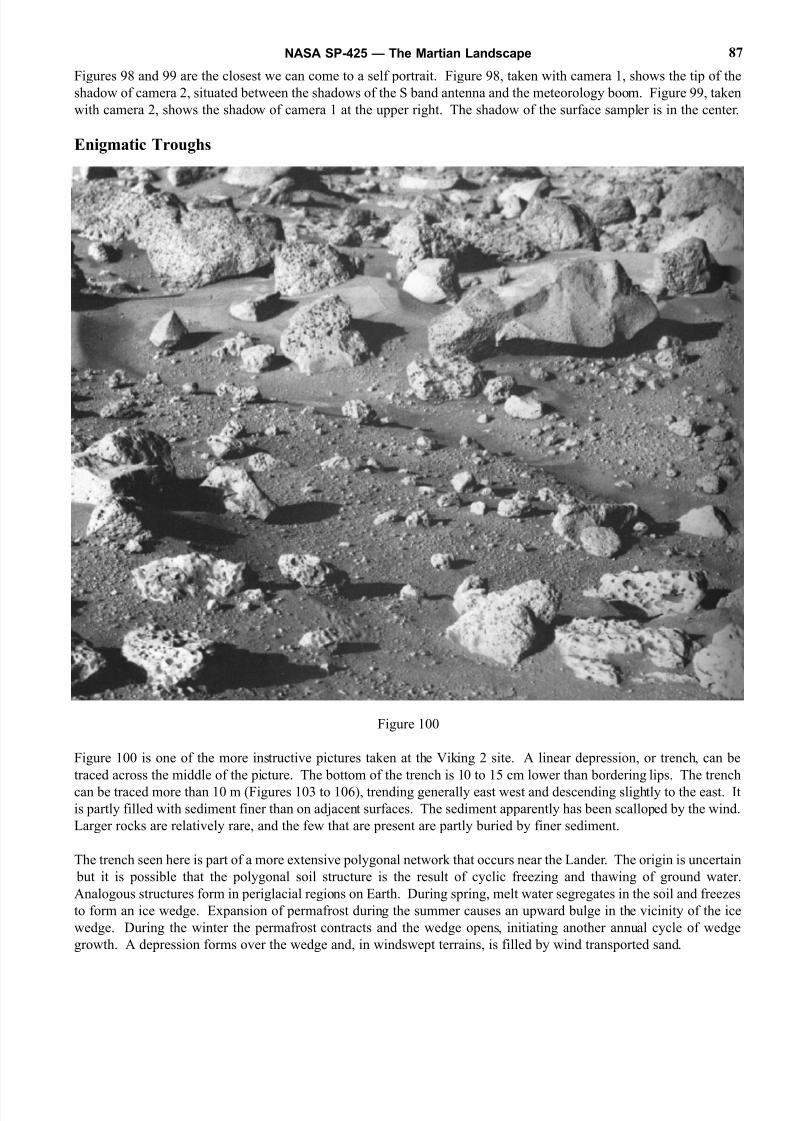
8/8/2019 The Martian Landscape
http://slidepdf.com/reader/full/the-martian-landscape 87/160
Figures 98 and 99 are the closest we can come to a self portrait. Figure 98, taken with camera 1, shows the tip of the
shadow of camera 2, situated between the shadows of the S band antenna and the meteorology boom. Figure 99, taken
with camera 2, shows the shadow of camera 1 at the upper right. The shadow of the surface sampler is in the center.
Enigmatic Troughs
Figure 100
Figure 100 is one of the more instructive pictures taken at the Viking 2 site. A linear depression, or trench, can be
traced across the middle of the picture. The bottom of the trench is 10 to 15 cm lower than bordering lips. The trench
can be traced more than 10 m (Figures 103 to 106), trending generally east west and descending slightly to the east. It
is partly filled with sediment finer than on adjacent surfaces. The sediment apparently has been scalloped by the wind
Larger rocks are relatively rare, and the few that are present are partly buried by finer sediment.
The trench seen here is part of a more extensive polygonal network that occurs near the Lander. The origin is uncertain
but it is possible that the polygonal soil structure is the result of cyclic freezing and thawing of ground water
Analogous structures form in periglacial regions on Earth. During spring, melt water segregates in the soil and freezes
to form an ice wedge. Expansion of permafrost during the summer causes an upward bulge in the vicinity of the ice
wedge. During the winter the permafrost contracts and the wedge opens, initiating another annual cycle of wedge
growth. A depression forms over the wedge and, in windswept terrains, is filled by wind transported sand.
NASA SP-425 — The Martian Landscape 87
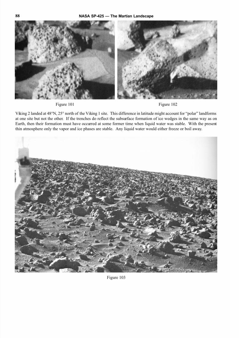
8/8/2019 The Martian Landscape
http://slidepdf.com/reader/full/the-martian-landscape 88/160
Viking 2 landed at 48°N, 25° north of the Viking 1 site. This difference in latitude might account for “polar” landforms
at one site but not the other. If the trenches do reflect the subsurface formation of ice wedges in the same way as onEarth, then their formation must have occurred at some former time when liquid water was stable. With the present
thin atmosphere only the vapor and ice phases are stable. Any liquid water would either freeze or boil away.
NASA SP-425 — The Martian Landscape88
Figure 102
Figure 103
Figure 101
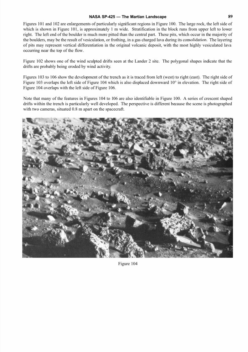
8/8/2019 The Martian Landscape
http://slidepdf.com/reader/full/the-martian-landscape 89/160
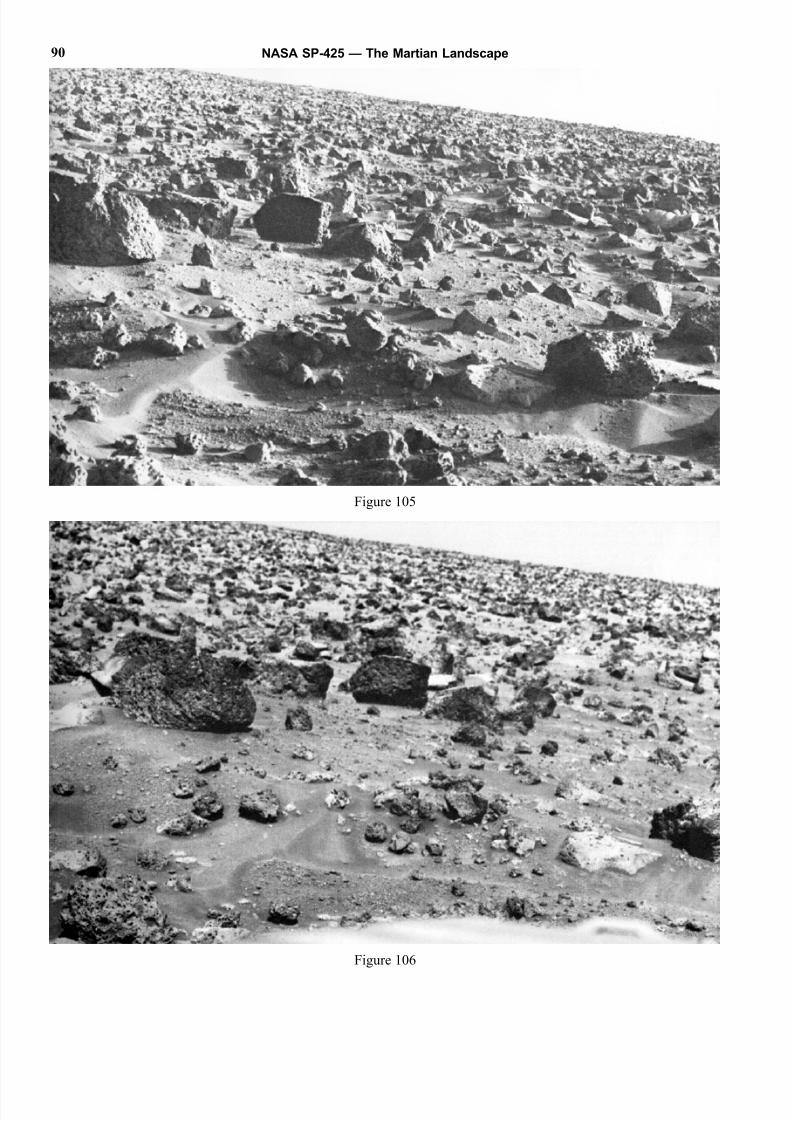
8/8/2019 The Martian Landscape
http://slidepdf.com/reader/full/the-martian-landscape 90/160
NASA SP-425 — The Martian Landscape90
Figure 105
Figure 106

8/8/2019 The Martian Landscape
http://slidepdf.com/reader/full/the-martian-landscape 91/160
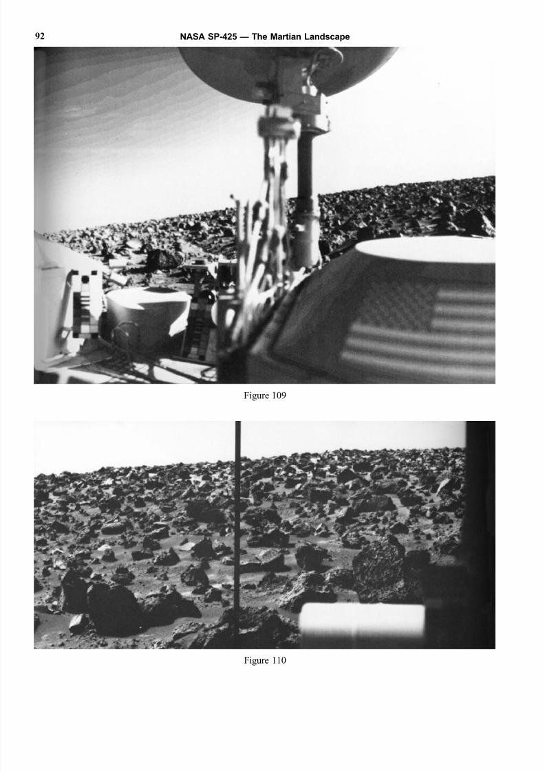
8/8/2019 The Martian Landscape
http://slidepdf.com/reader/full/the-martian-landscape 92/160
NASA SP-425 — The Martian Landscape92
Figure 109
Figure 110
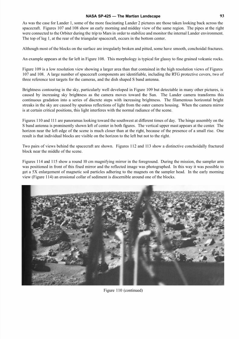
8/8/2019 The Martian Landscape
http://slidepdf.com/reader/full/the-martian-landscape 93/160
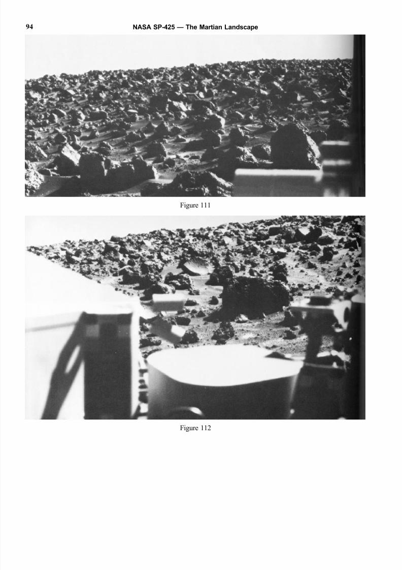
8/8/2019 The Martian Landscape
http://slidepdf.com/reader/full/the-martian-landscape 94/160
NASA SP-425 — The Martian Landscape94
Figure 111
Figure 112
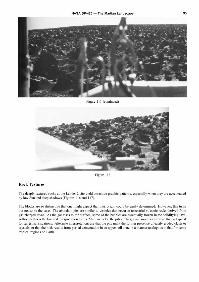
8/8/2019 The Martian Landscape
http://slidepdf.com/reader/full/the-martian-landscape 95/160
Rock Textures
The deeply textured rocks at the Lander 2 site yield attractive graphic patterns, especially when they are accentuated
by low Sun and deep shadows (Figures 116 and 117).
The blocks are so distinctive that one might expect that their origin could be easily determined. However, this turns
out not to be the case. The abundant pits are similar to vesicles that occur in terrestrial volcanic rocks derived from
gas charged lavas. As the gas rises to the surface, some of the bubbles are essentially frozen in the solidifying lava
Although this is the favored interpretation for the Martian rocks, the pits are larger and more widespread than is typical
for terrestrial situations. Alternate interpretations are that the pits mark the former presence of easily eroded clasts or
crystals, or that the rock results from partial cementation in an upper soil zone in a manner analogous to that for some
tropical regions on Earth.
NASA SP-425 — The Martian Landscape 95
Figure 111 (continued)
Figure 113
8/8/2019 The Martian Landscape
http://slidepdf.com/reader/full/the-martian-landscape 96/160
NASA SP-425 — The Martian Landscape96
Figure 114
Figure 115
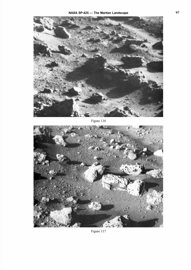
8/8/2019 The Martian Landscape
http://slidepdf.com/reader/full/the-martian-landscape 97/160
8/8/2019 The Martian Landscape
http://slidepdf.com/reader/full/the-martian-landscape 98/160
NASA SP-425 — The Martian Landscape98
Figure 118
Figure 119
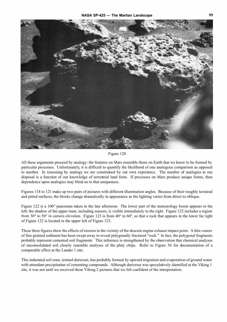
8/8/2019 The Martian Landscape
http://slidepdf.com/reader/full/the-martian-landscape 99/160
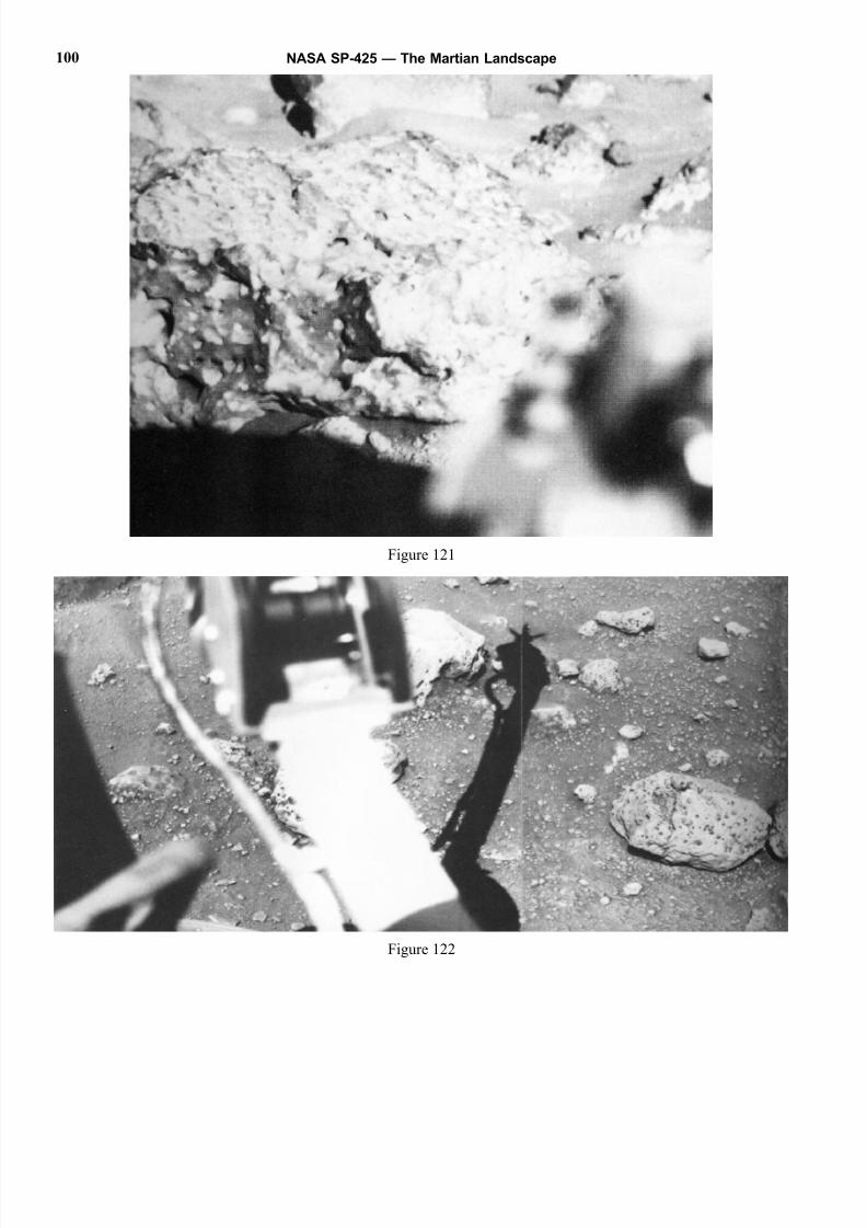
8/8/2019 The Martian Landscape
http://slidepdf.com/reader/full/the-martian-landscape 100/160
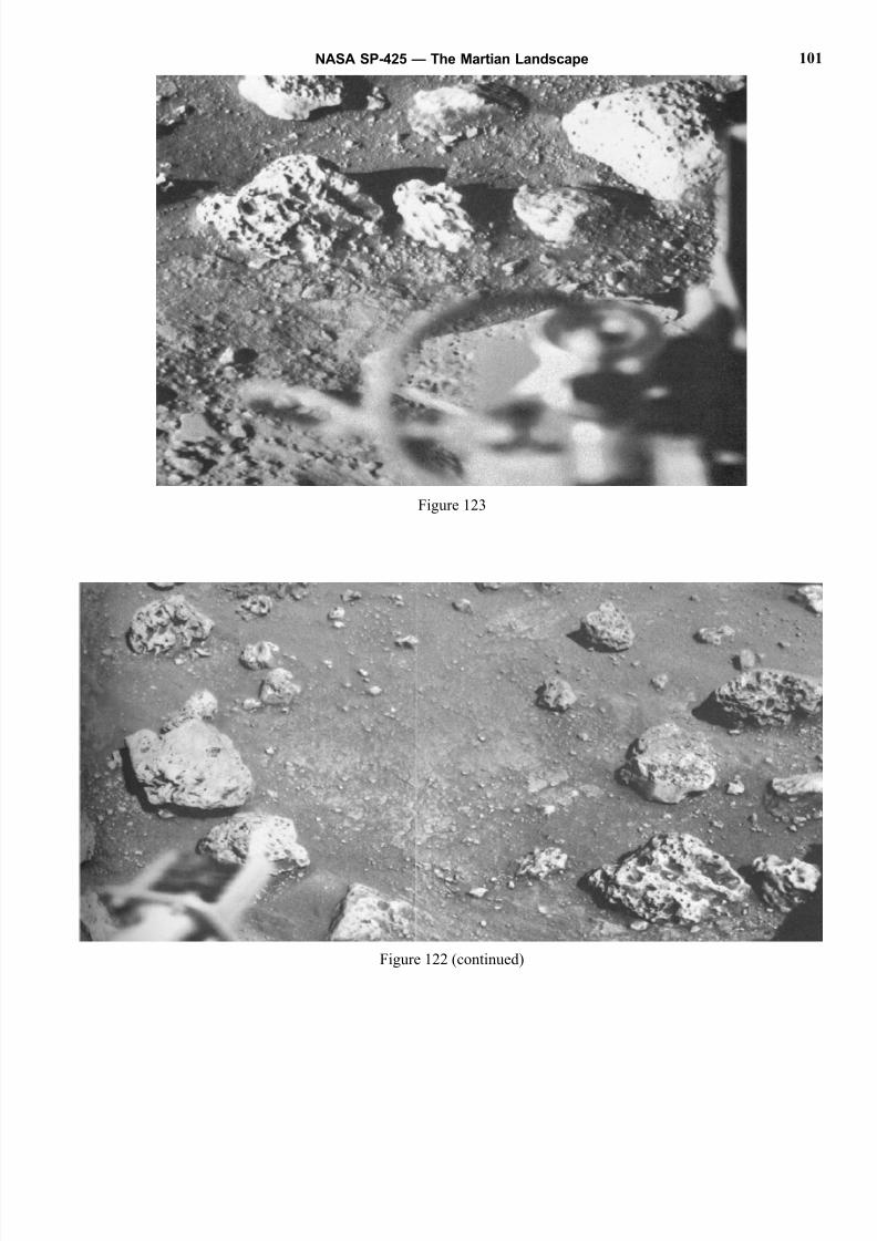
8/8/2019 The Martian Landscape
http://slidepdf.com/reader/full/the-martian-landscape 101/160
NASA SP-425 — The Martian Landscape 101
Figure 123
Figure 122 (continued)
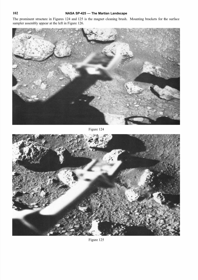
8/8/2019 The Martian Landscape
http://slidepdf.com/reader/full/the-martian-landscape 102/160
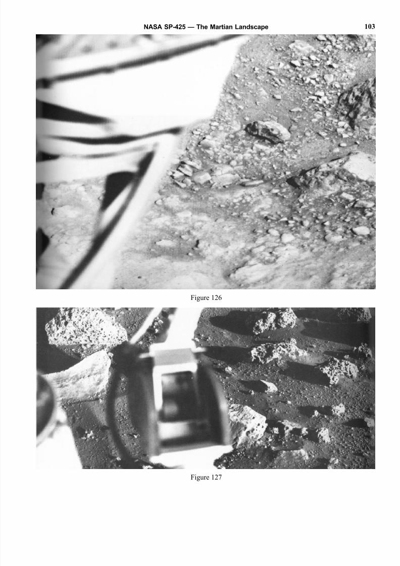
8/8/2019 The Martian Landscape
http://slidepdf.com/reader/full/the-martian-landscape 103/160
NASA SP-425 — The Martian Landscape 103
Figure 126
Figure 127
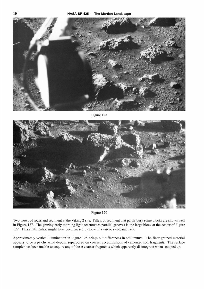
8/8/2019 The Martian Landscape
http://slidepdf.com/reader/full/the-martian-landscape 104/160
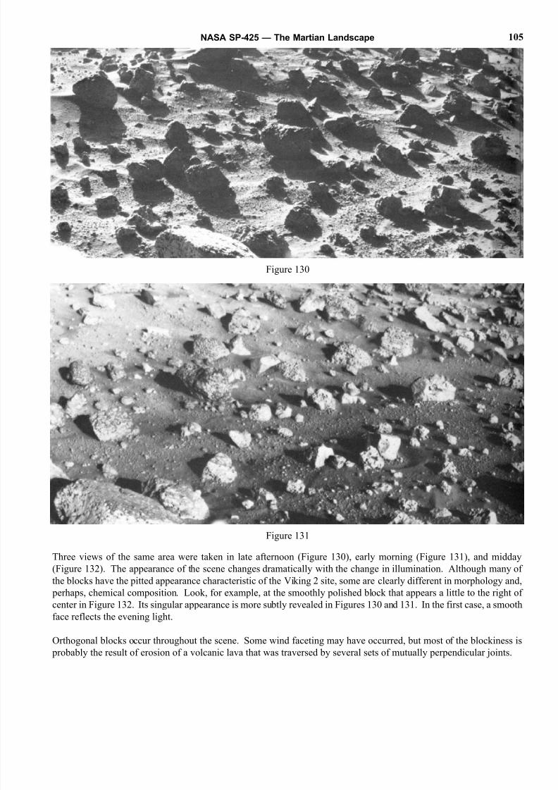
8/8/2019 The Martian Landscape
http://slidepdf.com/reader/full/the-martian-landscape 105/160
Three views of the same area were taken in late afternoon (Figure 130), early morning (Figure 131), and midday(Figure 132). The appearance of the scene changes dramatically with the change in illumination. Although many of
the blocks have the pitted appearance characteristic of the Viking 2 site, some are clearly different in morphology and
perhaps, chemical composition. Look, for example, at the smoothly polished block that appears a little to the right of
center in Figure 132. Its singular appearance is more subtly revealed in Figures 130 and 131. In the first case, a smooth
face reflects the evening light.
Orthogonal blocks occur throughout the scene. Some wind faceting may have occurred, but most of the blockiness is
probably the result of erosion of a volcanic lava that was traversed by several sets of mutually perpendicular joints.
NASA SP-425 — The Martian Landscape 105
Figure 130
Figure 131
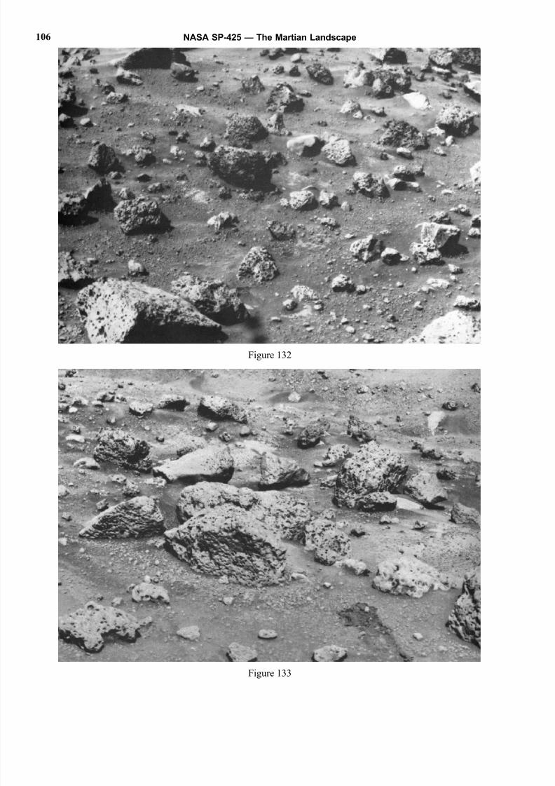
8/8/2019 The Martian Landscape
http://slidepdf.com/reader/full/the-martian-landscape 106/160
NASA SP-425 — The Martian Landscape106
Figure 132
Figure 133
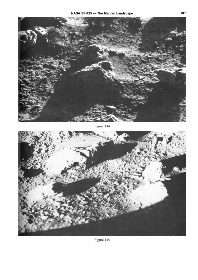
8/8/2019 The Martian Landscape
http://slidepdf.com/reader/full/the-martian-landscape 107/160
NASA SP-425 — The Martian Landscape 107
Figure 134
Figure 135
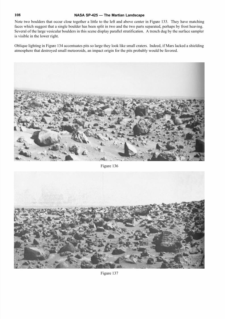
8/8/2019 The Martian Landscape
http://slidepdf.com/reader/full/the-martian-landscape 108/160
Note two boulders that occur close together a little to the left and above center in Figure 133. They have matching
faces which suggest that a single boulder has been split in two and the two parts separated, perhaps by frost heaving.
Several of the large vesicular boulders in this scene display parallel stratification. A trench dug by the surface sampler
is visible in the lower right.
Oblique lighting in Figure 134 accentuates pits so large they look like small craters. Indeed, if Mars lacked a shielding
atmosphere that destroyed small meteoroids, an impact origin for the pits probably would be favored.
NASA SP-425 — The Martian Landscape108
Figure 136
Figure 137
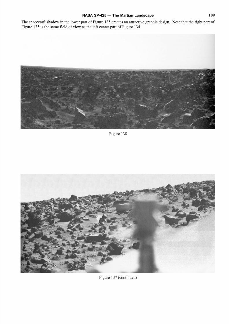
8/8/2019 The Martian Landscape
http://slidepdf.com/reader/full/the-martian-landscape 109/160
The spacecraft shadow in the lower part of Figure 135 creates an attractive graphic design. Note that the right part of
Figure 135 is the same field of view as the left center part of Figure 134.
NASA SP-425 — The Martian Landscape 109
Figure 138
Figure 137 (continued)
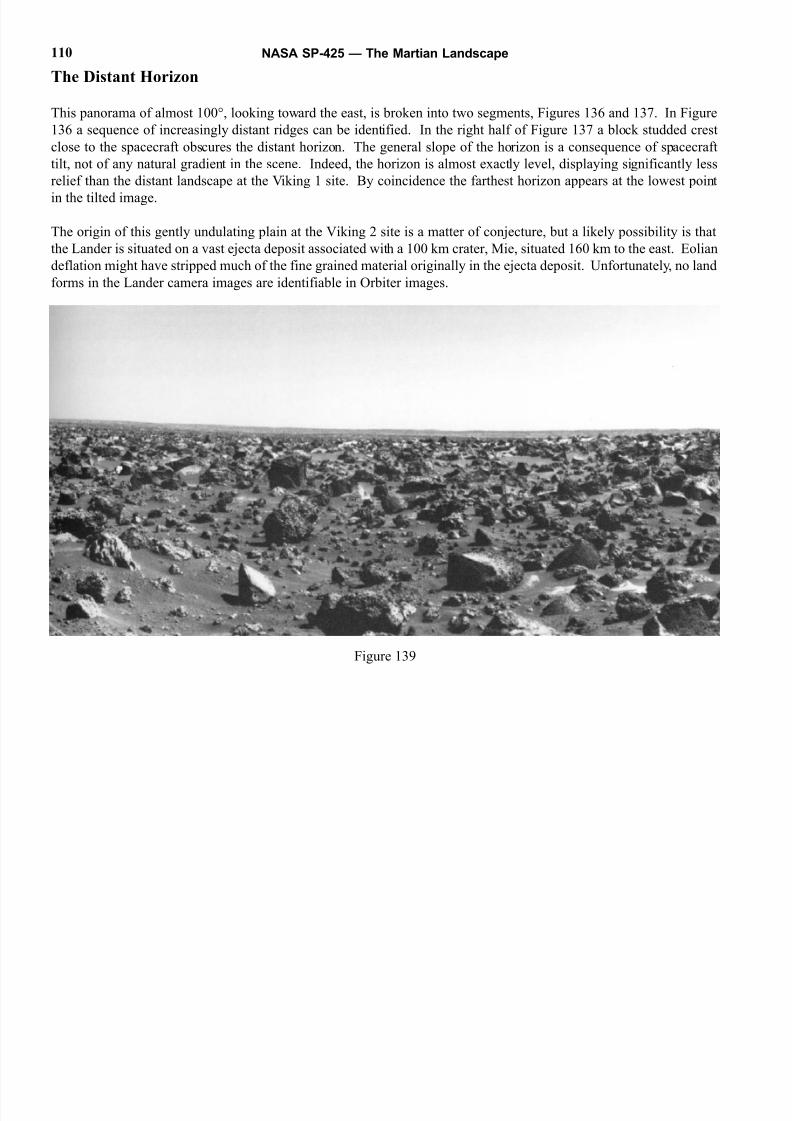
8/8/2019 The Martian Landscape
http://slidepdf.com/reader/full/the-martian-landscape 110/160
The Distant Horizon
This panorama of almost 100°, looking toward the east, is broken into two segments, Figures 136 and 137. In Figure
136 a sequence of increasingly distant ridges can be identified. In the right half of Figure 137 a block studded crest
close to the spacecraft obscures the distant horizon. The general slope of the horizon is a consequence of spacecraft
tilt, not of any natural gradient in the scene. Indeed, the horizon is almost exactly level, displaying significantly less
relief than the distant landscape at the Viking 1 site. By coincidence the farthest horizon appears at the lowest point
in the tilted image.
The origin of this gently undulating plain at the Viking 2 site is a matter of conjecture, but a likely possibility is that
the Lander is situated on a vast ejecta deposit associated with a 100 km crater, Mie, situated 160 km to the east. Eolian
deflation might have stripped much of the fine grained material originally in the ejecta deposit. Unfortunately, no land
forms in the Lander camera images are identifiable in Orbiter images.
Figure 139
NASA SP-425 — The Martian Landscape110
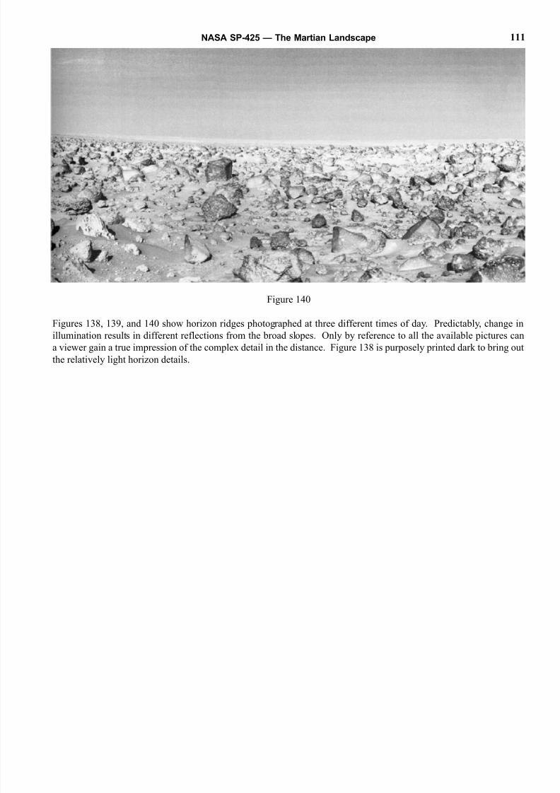
8/8/2019 The Martian Landscape
http://slidepdf.com/reader/full/the-martian-landscape 111/160
Figure 140
Figures 138, 139, and 140 show horizon ridges photographed at three different times of day. Predictably, change in
illumination results in different reflections from the broad slopes. Only by reference to all the available pictures can
a viewer gain a true impression of the complex detail in the distance. Figure 138 is purposely printed dark to bring out
the relatively light horizon details.
NASA SP-425 — The Martian Landscape 111
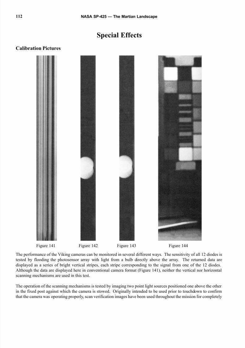
8/8/2019 The Martian Landscape
http://slidepdf.com/reader/full/the-martian-landscape 112/160
Special Effects
Calibration Pictures
The performance of the Viking cameras can be monitored in several different ways. The sensitivity of all 12 diodes is
tested by flooding the photosensor array with light from a bulb directly above the array. The returned data are
displayed as a series of bright vertical stripes, each stripe corresponding to the signal from one of the 12 diodes.
Although the data are displayed here in conventional camera format (Figure 141), neither the vertical nor horizontal
scanning mechanisms are used in this test.
The operation of the scanning mechanisms is tested by imaging two point light sources positioned one above the other
in the fixed post against which the camera is stowed. Originally intended to be used prior to touchdown to confirm
that the camera was operating properly, scan verification images have been used throughout the mission for completely
NASA SP-425 — The Martian Landscape112
Figure 141 Figure 142 Figure 143 Figure 144
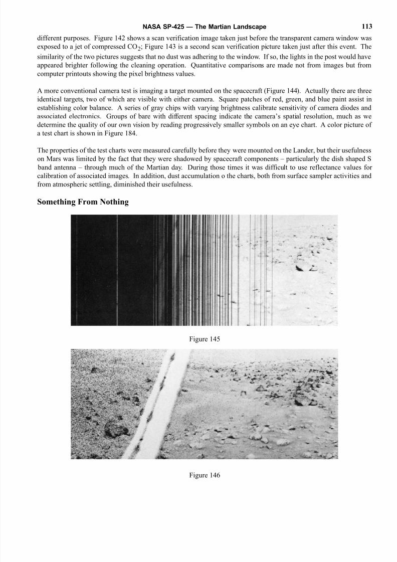
8/8/2019 The Martian Landscape
http://slidepdf.com/reader/full/the-martian-landscape 113/160
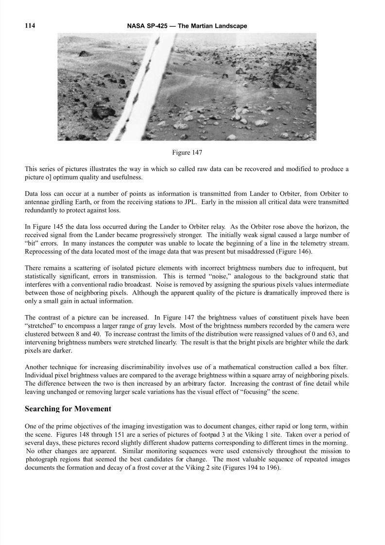
8/8/2019 The Martian Landscape
http://slidepdf.com/reader/full/the-martian-landscape 114/160
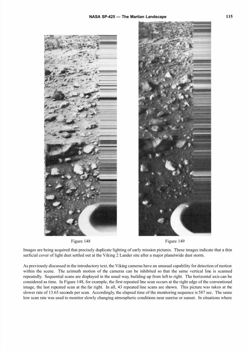
8/8/2019 The Martian Landscape
http://slidepdf.com/reader/full/the-martian-landscape 115/160
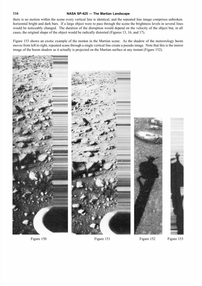
8/8/2019 The Martian Landscape
http://slidepdf.com/reader/full/the-martian-landscape 116/160
there is no motion within the scene every vertical line is identical, and the repeated line image comprises unbroken
horizontal bright and dark bars. If a large object were to pass through the scene the brightness levels in several lines
would be noticeably changed. The duration of the disruption would depend on the velocity of the object but, in all
cases, the original shape of the object would be radically distorted (Figures 13, 16, and 17).
Figure 153 shows an exotic example of the motion in the Martian scene. As the shadow of the meteorology boom
moves from left to right, repeated scans through a single vertical line create a pseudo image. Note that this is the mirror
image of the boom shadow as it actually is projected on the Martian surface at any instant (Figure 152).
NASA SP-425 — The Martian Landscape116
Figure 150 Figure 151 Figure 152 Figure 153
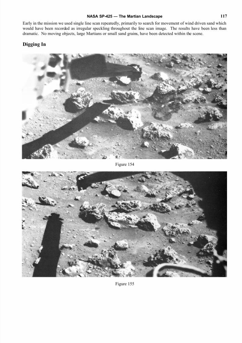
8/8/2019 The Martian Landscape
http://slidepdf.com/reader/full/the-martian-landscape 117/160
Early in the mission we used single line scan repeatedly, primarily to search for movement of wind driven sand which
would have been recorded as irregular speckling throughout the line scan image. The results have been less than
dramatic. No moving objects, large Martians or small sand grains, have been detected within the scene.
Digging In
Figure 154
Figure 155
NASA SP-425 — The Martian Landscape 117
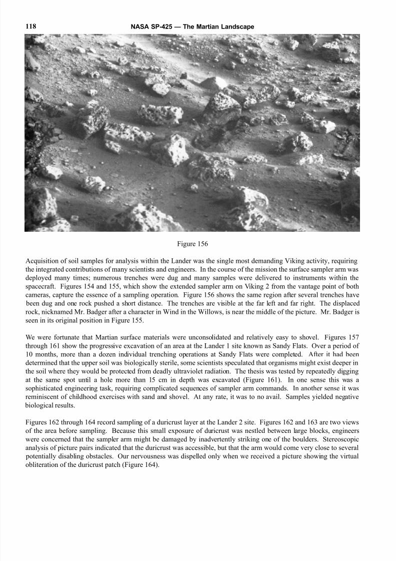
8/8/2019 The Martian Landscape
http://slidepdf.com/reader/full/the-martian-landscape 118/160
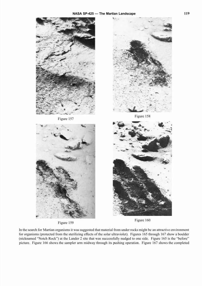
8/8/2019 The Martian Landscape
http://slidepdf.com/reader/full/the-martian-landscape 119/160
In the search for Martian organisms it was suggested that material from under rocks might be an attractive environment
for organisms (protected from the sterilizing effects of the solar ultraviolet). Figures 165 through 167 show a boulder
(nicknamed “Notch Rock”) at the Lander 2 site that was successfully nudged to one side. Figure 165 is the “before”
picture. Figure 166 shows the sampler arm midway through its pushing operation. Figure 167 shows the completed
NASA SP-425 — The Martian Landscape 119
Figure 157Figure 158
Figure 159Figure 160
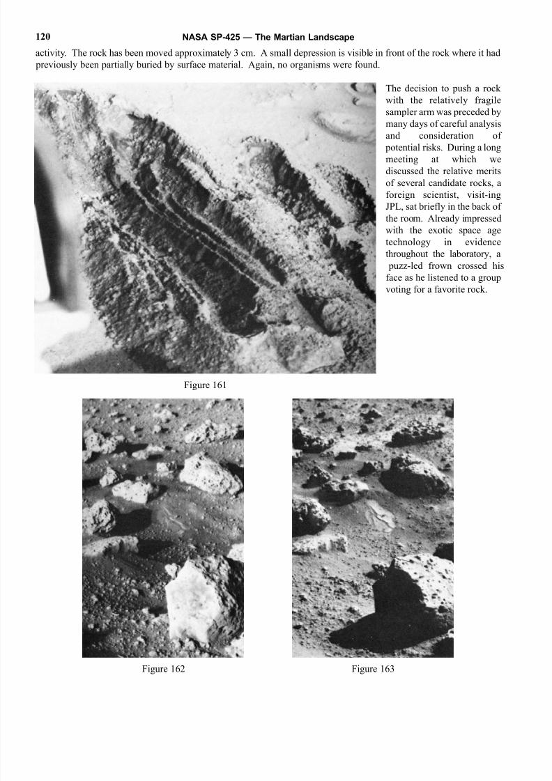
8/8/2019 The Martian Landscape
http://slidepdf.com/reader/full/the-martian-landscape 120/160
activity. The rock has been moved approximately 3 cm. A small depression is visible in front of the rock where it had
previously been partially buried by surface material. Again, no organisms were found.
The decision to push a rock
with the relatively fragile
sampler arm was preceded by
many days of careful analysis
and consideration of potential risks. During a long
meeting at which we
discussed the relative merits
of several candidate rocks, a
foreign scientist, visit-ing
JPL, sat briefly in the back of
the room. Already impressed
with the exotic space age
technology in evidence
throughout the laboratory, a
puzz-led frown crossed his
face as he listened to a group
voting for a favorite rock.
NASA SP-425 — The Martian Landscape120
Figure 161
Figure 162 Figure 163
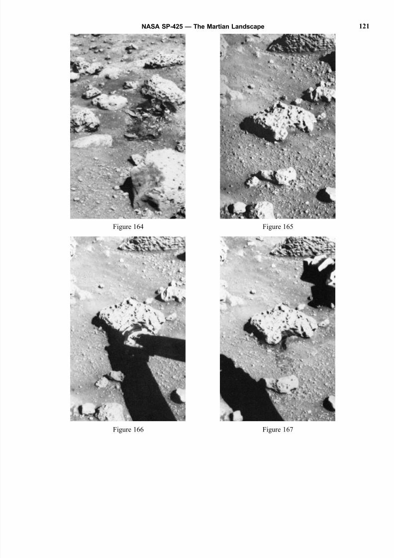
8/8/2019 The Martian Landscape
http://slidepdf.com/reader/full/the-martian-landscape 121/160
NASA SP-425 — The Martian Landscape 121
Figure 164
Figure 166 Figure 167
Figure 165
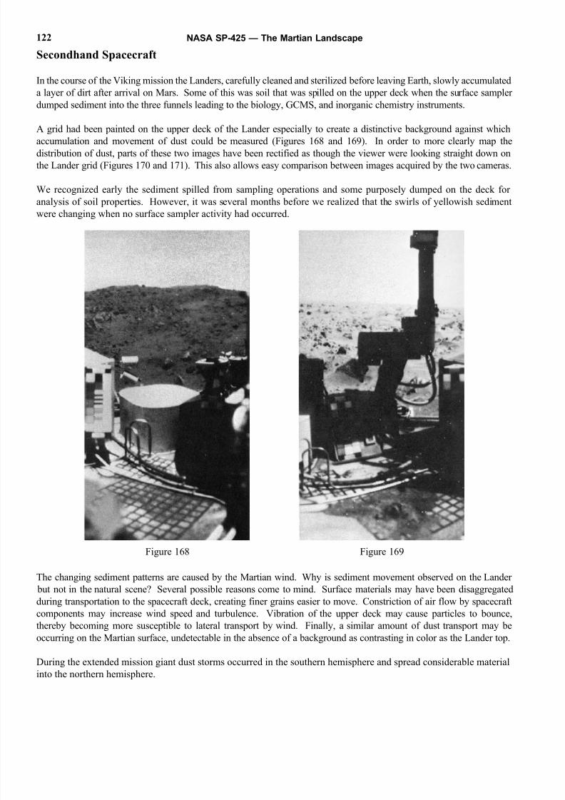
8/8/2019 The Martian Landscape
http://slidepdf.com/reader/full/the-martian-landscape 122/160
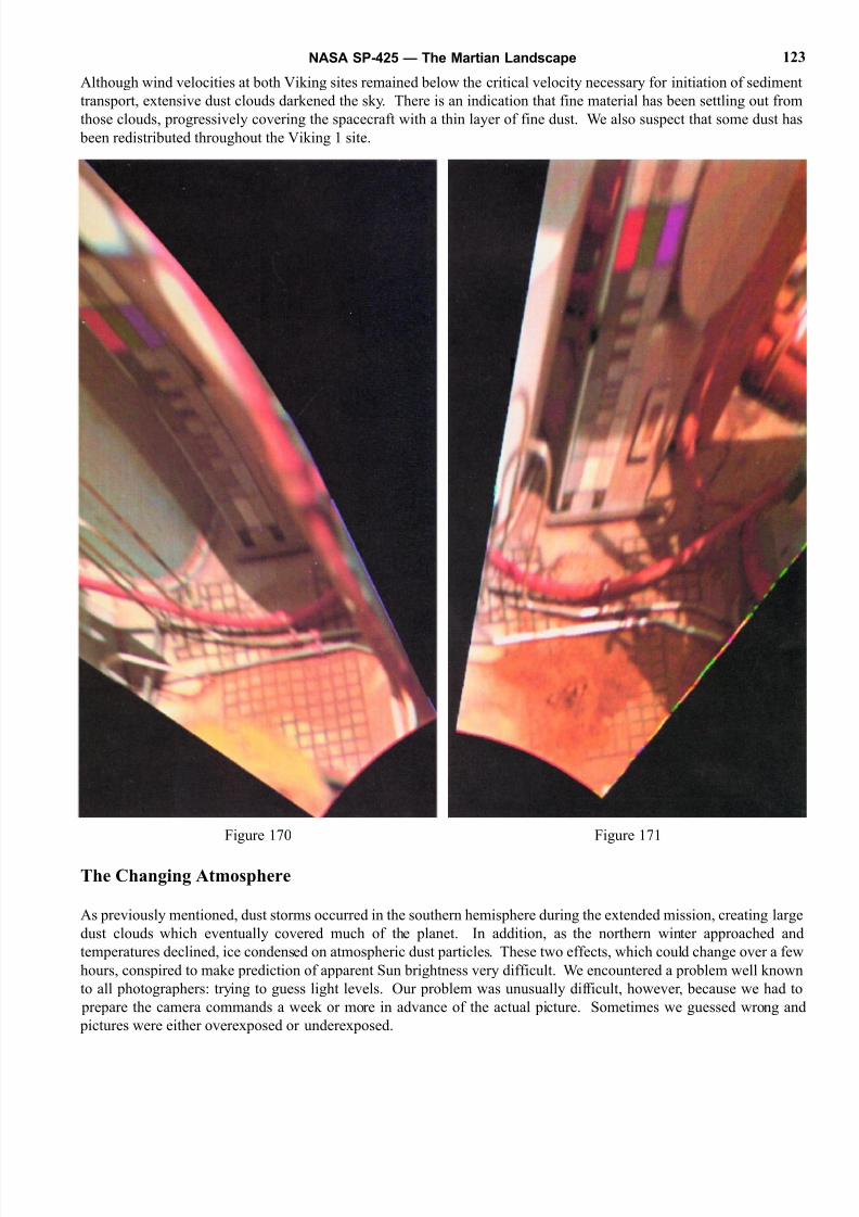
8/8/2019 The Martian Landscape
http://slidepdf.com/reader/full/the-martian-landscape 123/160
Although wind velocities at both Viking sites remained below the critical velocity necessary for initiation of sediment
transport, extensive dust clouds darkened the sky. There is an indication that fine material has been settling out from
those clouds, progressively covering the spacecraft with a thin layer of fine dust. We also suspect that some dust has
been redistributed throughout the Viking 1 site.
The Changing Atmosphere
As previously mentioned, dust storms occurred in the southern hemisphere during the extended mission, creating large
dust clouds which eventually covered much of the planet. In addition, as the northern winter approached and
temperatures declined, ice condensed on atmospheric dust particles. These two effects, which could change over a few
hours, conspired to make prediction of apparent Sun brightness very difficult. We encountered a problem well known
to all photographers: trying to guess light levels. Our problem was unusually difficult, however, because we had to
prepare the camera commands a week or more in advance of the actual picture. Sometimes we guessed wrong and
pictures were either overexposed or underexposed.
NASA SP-425 — The Martian Landscape 123
Figure 170 Figure 171
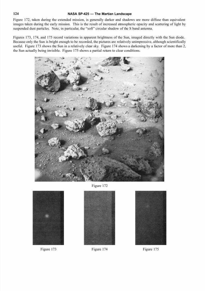
8/8/2019 The Martian Landscape
http://slidepdf.com/reader/full/the-martian-landscape 124/160
Figure 172, taken during the extended mission, is generally darker and shadows are more diffuse than equivalent
images taken during the early mission. This is the result of increased atmospheric opacity and scattering of light by
suspended dust particles. Note, in particular, the “soft” circular shadow of the S band antenna.
Figures 173, 174, and 175 record variations in apparent brightness of the Sun, imaged directly with the Sun diode.
Because only the Sun is bright enough to be recorded, the pictures are relatively unimpressive, although scientifically
useful. Figure 173 shows the Sun in a relatively clear sky. Figure 174 shows a darkening by a factor of more than 2,
the Sun actually being invisible. Figure 175 shows a partial return to clear conditions.
NASA SP-425 — The Martian Landscape124
Figure 172
Figure 173 Figure 174 Figure 175
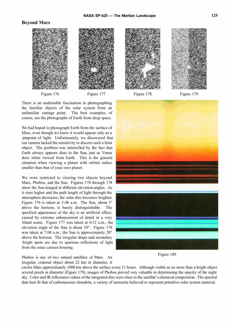
8/8/2019 The Martian Landscape
http://slidepdf.com/reader/full/the-martian-landscape 125/160
Beyond Mars
There is an undeniable fascination in photographing
the familiar objects of the solar system from an
unfamiliar vantage point. The best examples, of
course, are the photographs of Earth from deep space.
We had hoped to photograph Earth from the surface of
Mars, even though we knew it would appear only as a
pinpoint of light. Unfortunately, we discovered that
our camera lacked the sensitivity to discern such a faint
object. The problem was intensified by the fact that
Earth always appears dose to the Sun, just as Venus
does when viewed from Earth. This is the general
situation when viewing a planet with orbital radius
smaller than that of your own planet.
We were restricted to viewing two objects beyond
Mars, Phobos, and the Sun. Figures 176 through 178
show the Sun imaged at different elevation angles. As
it rises higher and the path length of light through the
atmosphere decreases, the solar disc becomes brighter.
Figure 176 is taken at 5:48 a.m. The Sun, about 5°
above the horizon, is barely distinguishable. The
speckled appearance of the sky is an artificial effect,
caused by extreme enhancement of detail in a very
bland scene. Figure 177 was taken at 6:12 a.m.; the
elevation angle of the Sun is about 10°. Figure 178
was taken at 7:00 a.m.; the Sun is approximately 20°
above the horizon. The irregular shape and secondary
bright spots are due to spurious reflections of light
from the outer camera housing.
Phobos is one of two natural satellites of Mars. An
irregular, cratered object about 22 km in diameter, it
circles Mars approximately 1000 km above the surface every 11 hours. Although visible as no more than a bright object
several pixels in diameter (Figure 179), images of Phobos proved very valuable in determining the opacity of the night
sky. Color and IR reflectance values of the integrated disc were clues to the satellite’s chemical composition. The spectral
data best fit that of carbonaceous chondrite, a variety of meteorite believed to represent primitive solar system material.
NASA SP-425 — The Martian Landscape 125
Figure 176
Figure 180
Figure 177 Figure 178 Figure 179
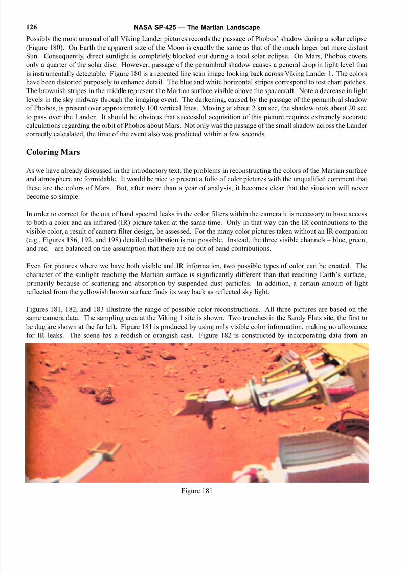
8/8/2019 The Martian Landscape
http://slidepdf.com/reader/full/the-martian-landscape 126/160
Possibly the most unusual of all Viking Lander pictures records the passage of Phobos’ shadow during a solar eclipse
(Figure 180). On Earth the apparent size of the Moon is exactly the same as that of the much larger but more distant
Sun. Consequently, direct sunlight is completely blocked out during a total solar eclipse. On Mars, Phobos covers
only a quarter of the solar disc. However, passage of the penumbral shadow causes a general drop in light level that
is instrumentally detectable. Figure 180 is a repeated line scan image looking back across Viking Lander 1. The colors
have been distorted purposely to enhance detail. The blue and white horizontal stripes correspond to test chart patches.
The brownish stripes in the middle represent the Martian surface visible above the spacecraft. Note a decrease in light
levels in the sky midway through the imaging event. The darkening, caused by the passage of the penumbral shadowof Phobos, is present over approximately 100 vertical lines. Moving at about 2 km sec, the shadow took about 20 sec
to pass over the Lander. It should be obvious that successful acquisition of this picture requires extremely accurate
calculations regarding the orbit of Phobos about Mars. Not only was the passage of the small shadow across the Lander
correctly calculated, the time of the event also was predicted within a few seconds.
Coloring Mars
As we have already discussed in the introductory text, the problems in reconstructing the colors of the Martian surface
and atmosphere are formidable. It would be nice to present a folio of color pictures with the unqualified comment that
these are the colors of Mars. But, after more than a year of analysis, it becomes clear that the situation will never
become so simple.
In order to correct for the out of band spectral leaks in the color filters within the camera it is necessary to have access
to both a color and an infrared (IR) picture taken at the same time. Only in that way can the IR contributions to the
visible color, a result of camera filter design, be assessed. For the many color pictures taken without an IR companion
(e.g., Figures 186, 192, and 198) detailed calibration is not possible. Instead, the three visible channels – blue, green,
and red – are balanced on the assumption that there are no out of band contributions.
Even for pictures where we have both visible and IR information, two possible types of color can be created. The
character of the sunlight reaching the Martian surface is significantly different than that reaching Earth’s surface,
primarily because of scattering and absorption by suspended dust particles. In addition, a certain amount of light
reflected from the yellowish brown surface finds its way back as reflected sky light.
Figures 181, 182, and 183 illustrate the range of possible color reconstructions. All three pictures are based on the
same camera data. The sampling area at the Viking 1 site is shown. Two trenches in the Sandy Flats site, the first to
be dug are shown at the far left. Figure 181 is produced by using only visible color information, making no allowance
for IR leaks. The scene has a reddish or orangish cast. Figure 182 is constructed by incorporating data from an
NASA SP-425 — The Martian Landscape126
Figure 181
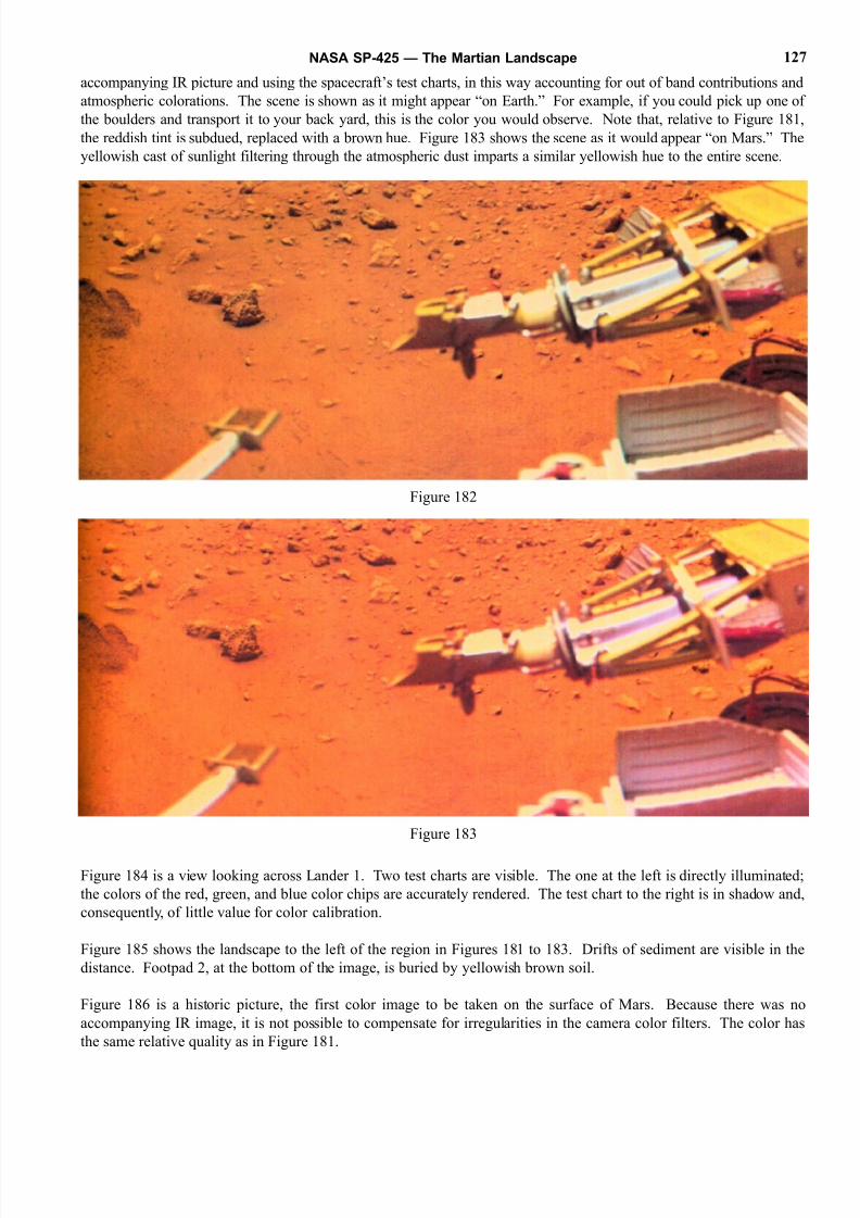
8/8/2019 The Martian Landscape
http://slidepdf.com/reader/full/the-martian-landscape 127/160
accompanying IR picture and using the spacecraft’s test charts, in this way accounting for out of band contributions and
atmospheric colorations. The scene is shown as it might appear “on Earth.” For example, if you could pick up one of
the boulders and transport it to your back yard, this is the color you would observe. Note that, relative to Figure 181
the reddish tint is subdued, replaced with a brown hue. Figure 183 shows the scene as it would appear “on Mars.” The
yellowish cast of sunlight filtering through the atmospheric dust imparts a similar yellowish hue to the entire scene.
Figure 184 is a view looking across Lander 1. Two test charts are visible. The one at the left is directly illuminated;
the colors of the red, green, and blue color chips are accurately rendered. The test chart to the right is in shadow and
consequently, of little value for color calibration.
Figure 185 shows the landscape to the left of the region in Figures 181 to 183. Drifts of sediment are visible in the
distance. Footpad 2, at the bottom of the image, is buried by yellowish brown soil.
Figure 186 is a historic picture, the first color image to be taken on the surface of Mars. Because there was no
accompanying IR image, it is not possible to compensate for irregularities in the camera color filters. The color has
the same relative quality as in Figure 181.
NASA SP-425 — The Martian Landscape 127
Figure 182
Figure 183
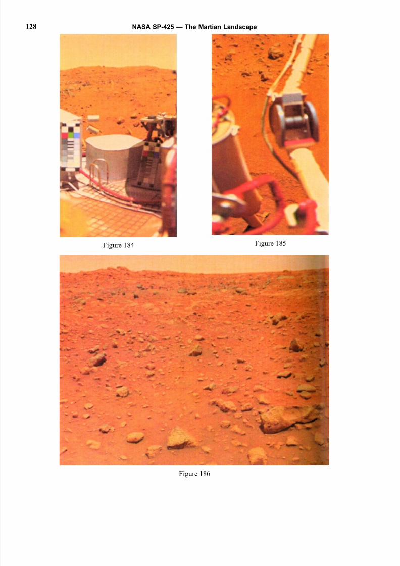
8/8/2019 The Martian Landscape
http://slidepdf.com/reader/full/the-martian-landscape 128/160
NASA SP-425 — The Martian Landscape128
Figure 184 Figure 185
Figure 186
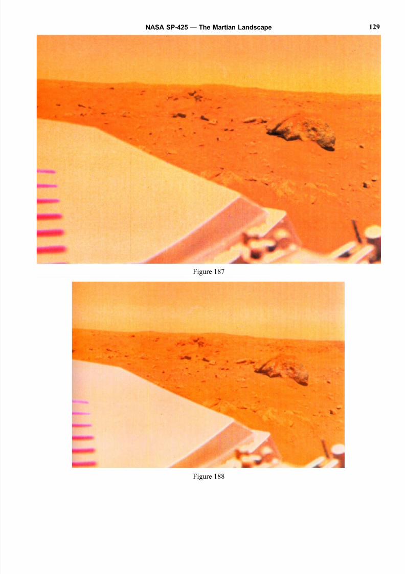
8/8/2019 The Martian Landscape
http://slidepdf.com/reader/full/the-martian-landscape 129/160
NASA SP-425 — The Martian Landscape 129
Figure 187
Figure 188
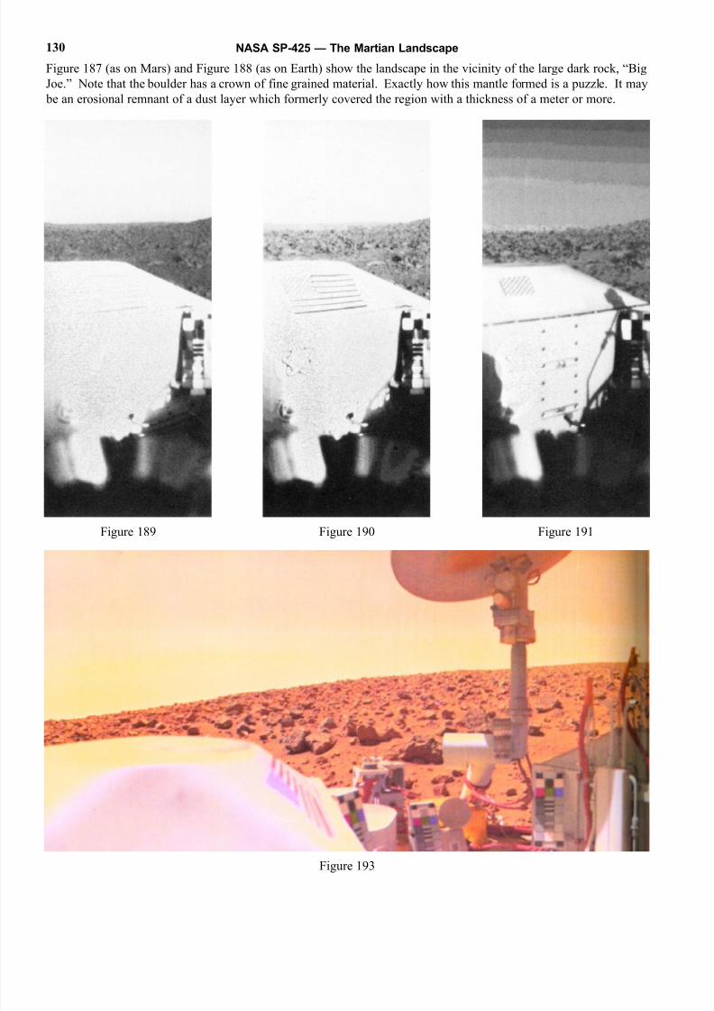
8/8/2019 The Martian Landscape
http://slidepdf.com/reader/full/the-martian-landscape 130/160
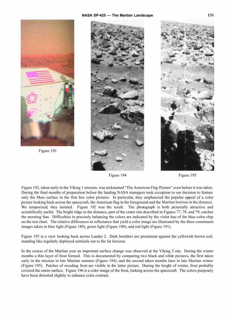
8/8/2019 The Martian Landscape
http://slidepdf.com/reader/full/the-martian-landscape 131/160
Figure 192, taken early in the Viking 1 mission, was nicknamed “The American Flag Picture” even before it was taken.
During the final months of preparation before the landing NASA managers took exception to our decision to feature
only the Mars surface in the first few color pictures. In particular, they emphasized the popular appeal of a color
picture looking back across the spacecraft, the American flag in the foreground and the Martian horizon in the distance.
We temporized; they insisted. Figure 192 was the result. The photograph is both pictorially attractive and
scientifically useful. The bright ridge in the distance, part of the crater rim described in Figures 77, 78, and 79, catches
the morning Sun. Difficulties in precisely balancing the colors are indicated by the violet hue of the blue color chip
on the test chart. The relative differences in reflectance that yield a color image are illustrated by the three constituent
images taken in blue light (Figure 189), green light (Figure 190), and red light (Figure 191).
Figure 193 is a view looking back across Lander 2. Dark boulders are prominent against the yellowish brown soil
standing like regularly deployed sentinels out to the far horizon.
In the course of the Martian year an important surface change was observed at the Viking 2 site. During the winter
months a thin layer of frost formed. This is documented by comparing two black and white pictures, the first taken
early in the mission in late Martian summer (Figure 194), and the second taken months later in late Martian winter
(Figure 195). Patches of receding frost are visible in the latter picture. During the height of winter, frost probably
covered the entire surface. Figure 196 is a color image of the frost, looking across the spacecraft. The colors purposely
have been distorted slightly to enhance color contrast.
NASA SP-425 — The Martian Landscape 131
Figure 192
Figure 194 Figure 195
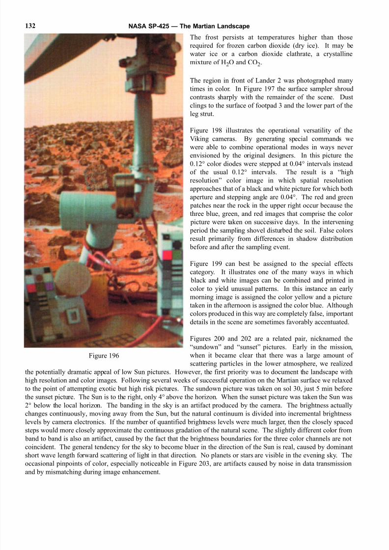
8/8/2019 The Martian Landscape
http://slidepdf.com/reader/full/the-martian-landscape 132/160
The frost persists at temperatures higher than those
required for frozen carbon dioxide (dry ice). It may be
water ice or a carbon dioxide clathrate, a crystalline
mixture of H2O and CO2.
The region in front of Lander 2 was photographed many
times in color. In Figure 197 the surface sampler shroud
contrasts sharply with the remainder of the scene. Dustclings to the surface of footpad 3 and the lower part of the
leg strut.
Figure 198 illustrates the operational versatility of the
Viking cameras. By generating special commands we
were able to combine operational modes in ways never
envisioned by the original designers. In this picture the
0.12° color diodes were stepped at 0.04° intervals instead
of the usual 0.12° intervals. The result is a “high
resolution” color image in which spatial resolution
approaches that of a black and white picture for which both
aperture and stepping angle are 0.04°. The red and green
patches near the rock in the upper right occur because the
three blue, green, and red images that comprise the color
picture were taken on successive days. In the intervening
period the sampling shovel disturbed the soil. False colors
result primarily from differences in shadow distribution
before and after the sampling event.
Figure 199 can best be assigned to the special effects
category. It illustrates one of the many ways in which
black and white images can be combined and printed in
color to yield unusual patterns. In this instance an earlymorning image is assigned the color yellow and a picture
taken in the afternoon is assigned the color blue. Although
colors produced in this way are completely false, important
details in the scene are sometimes favorably accentuated.
Figures 200 and 202 are a related pair, nicknamed the
“sundown” and “sunset” pictures. Early in the mission,
when it became clear that there was a large amount of
scattering particles in the lower atmosphere, we realized
the potentially dramatic appeal of low Sun pictures. However, the first priority was to document the landscape with
high resolution and color images. Following several weeks of successful operation on the Martian surface we relaxed
to the point of attempting exotic but high risk pictures. The sundown picture was taken on sol 30, just 5 min before
the sunset picture. The Sun is to the right, only 4° above the horizon. When the sunset picture was taken the Sun was
2° below the local horizon. The banding in the sky is an artifact produced by the camera. The brightness actually
changes continuously, moving away from the Sun, but the natural continuum is divided into incremental brightness
levels by camera electronics. If the number of quantified brightness levels were much larger, then the closely spaced
steps would more closely approximate the continuous gradation of the natural scene. The slightly different color from
band to band is also an artifact, caused by the fact that the brightness boundaries for the three color channels are not
coincident. The general tendency for the sky to become bluer in the direction of the Sun is real, caused by dominant
short wave length forward scattering of light in that direction. No planets or stars are visible in the evening sky. The
occasional pinpoints of color, especially noticeable in Figure 203, are artifacts caused by noise in data transmission
and by mismatching during image enhancement.
NASA SP-425 — The Martian Landscape132
Figure 196
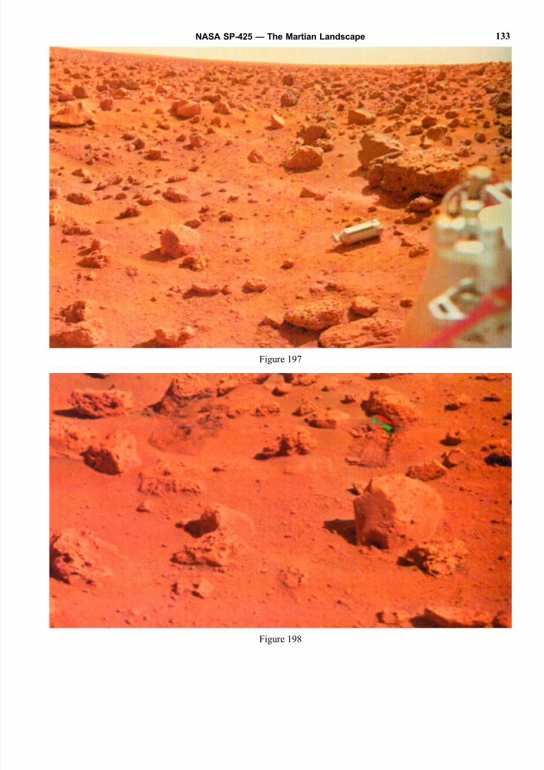
8/8/2019 The Martian Landscape
http://slidepdf.com/reader/full/the-martian-landscape 133/160
NASA SP-425 — The Martian Landscape 133
Figure 197
Figure 198
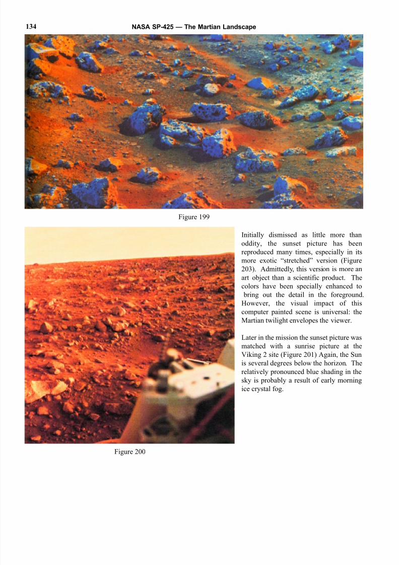
8/8/2019 The Martian Landscape
http://slidepdf.com/reader/full/the-martian-landscape 134/160
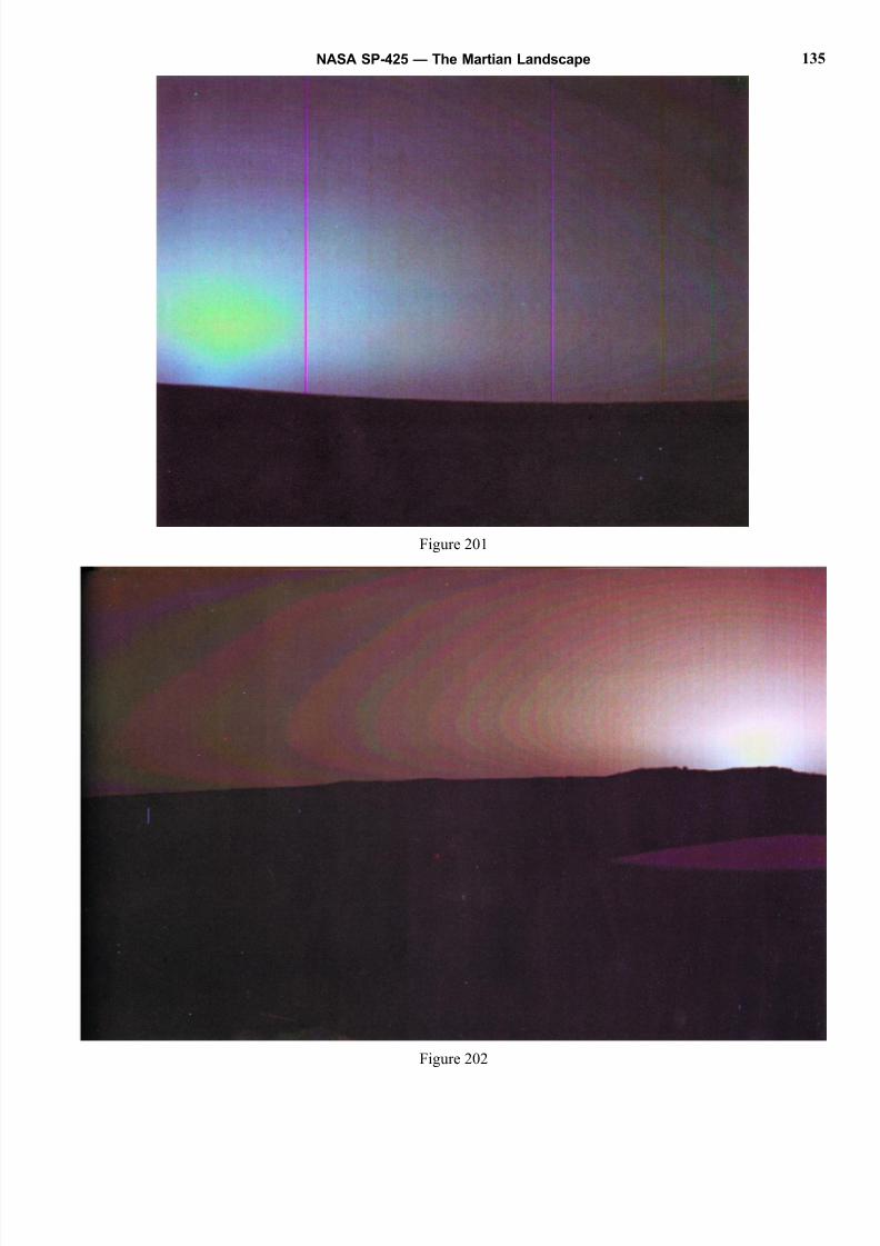
8/8/2019 The Martian Landscape
http://slidepdf.com/reader/full/the-martian-landscape 135/160
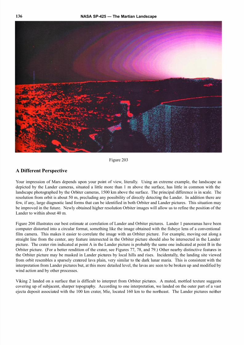
8/8/2019 The Martian Landscape
http://slidepdf.com/reader/full/the-martian-landscape 136/160
Figure 203
A Different Perspective
Your impression of Mars depends upon your point of view, literally. Using an extreme example, the landscape asdepicted by the Lander cameras, situated a little more than 1 m above the surface, has little in common with the
landscape photographed by the Orbiter cameras, 1500 km above the surface. The principal difference is in scale. The
resolution from orbit is about 50 m, precluding any possibility of directly detecting the Lander. In addition there are
few, if any, large diagnostic land forms that can be identified in both Orbiter and Lander pictures. This situation may
be improved in the future. Newly obtained higher resolution Orbiter images will allow us to refine the position of the
Lander to within about 40 m.
Figure 204 illustrates our best estimate at correlation of Lander and Orbiter pictures. Lander 1 panoramas have been
computer distorted into a circular format, something like the image obtained with the fisheye lens of a conventional
film camera. This makes it easier to correlate the image with an Orbiter picture. For example, moving out along a
straight line from the center, any feature intersected in the Orbiter picture should also be intersected in the Lander
picture. The crater rim indicated at point A in the Lander picture is probably the same one indicated at point B in the
Orbiter picture. (For a better rendition of the crater, see Figures 77, 78, and 79.) Other nearby distinctive features in
the Orbiter picture may be masked in Lander pictures by local hills and rises. Incidentally, the landing site viewed
from orbit resembles a sparsely cratered lava plain, very similar to the dark lunar maria. This is consistent with the
interpretation from Lander pictures but, at this more detailed level, the lavas are seen to be broken up and modified by
wind action and by other processes.
Viking 2 landed on a surface that is difficult to interpret from Orbiter pictures. A muted, mottled texture suggests
covering up of subjacent, sharper topography. According to one interpretation, we landed on the outer part of a vast
ejecta deposit associated with the 100 km crater, Mie, located 160 km to the northeast. The Lander pictures neither
NASA SP-425 — The Martian Landscape136
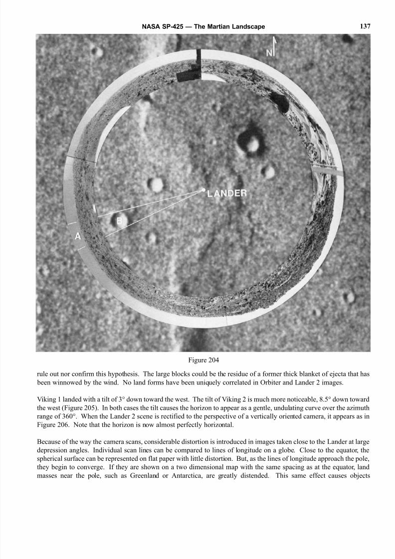
8/8/2019 The Martian Landscape
http://slidepdf.com/reader/full/the-martian-landscape 137/160
rule out nor confirm this hypothesis. The large blocks could be the residue of a former thick blanket of ejecta that has
been winnowed by the wind. No land forms have been uniquely correlated in Orbiter and Lander 2 images.
Viking 1 landed with a tilt of 3° down toward the west. The tilt of Viking 2 is much more noticeable, 8.5° down toward
the west (Figure 205). In both cases the tilt causes the horizon to appear as a gentle, undulating curve over the azimuth
range of 360°. When the Lander 2 scene is rectified to the perspective of a vertically oriented camera, it appears as in
Figure 206. Note that the horizon is now almost perfectly horizontal.
Because of the way the camera scans, considerable distortion is introduced in images taken close to the Lander at large
depression angles. Individual scan lines can be compared to lines of longitude on a globe. Close to the equator, the
spherical surface can be represented on flat paper with little distortion. But, as the lines of longitude approach the pole
they begin to converge. If they are shown on a two dimensional map with the same spacing as at the equator, land
masses near the pole, such as Greenland or Antarctica, are greatly distended. This same effect causes objects
NASA SP-425 — The Martian Landscape 137
Figure 204
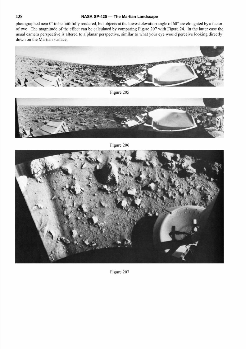
8/8/2019 The Martian Landscape
http://slidepdf.com/reader/full/the-martian-landscape 138/160
photographed near 0° to be faithfully rendered, but objects at the lowest elevation angle of 60° are elongated by a factor
of two. The magnitude of the effect can be calculated by comparing Figure 207 with Figure 24. In the latter case the
usual camera perspective is altered to a planar perspective, similar to what your eye would perceive looking directly
down on the Martian surface.
Figure 205
Figure 206
Figure 207
NASA SP-425 — The Martian Landscape138
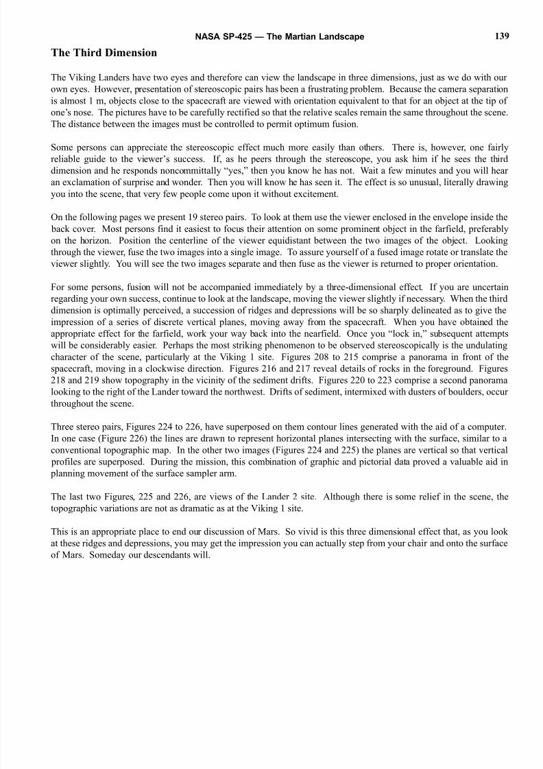
8/8/2019 The Martian Landscape
http://slidepdf.com/reader/full/the-martian-landscape 139/160
The Third Dimension
The Viking Landers have two eyes and therefore can view the landscape in three dimensions, just as we do with our
own eyes. However, presentation of stereoscopic pairs has been a frustrating problem. Because the camera separation
is almost 1 m, objects close to the spacecraft are viewed with orientation equivalent to that for an object at the tip of
one’s nose. The pictures have to be carefully rectified so that the relative scales remain the same throughout the scene
The distance between the images must be controlled to permit optimum fusion.
Some persons can appreciate the stereoscopic effect much more easily than others. There is, however, one fairly
reliable guide to the viewer’s success. If, as he peers through the stereoscope, you ask him if he sees the third
dimension and he responds noncommittally “yes,” then you know he has not. Wait a few minutes and you will hear
an exclamation of surprise and wonder. Then you will know he has seen it. The effect is so unusual, literally drawing
you into the scene, that very few people come upon it without excitement.
On the following pages we present 19 stereo pairs. To look at them use the viewer enclosed in the envelope inside the
back cover. Most persons find it easiest to focus their attention on some prominent object in the farfield, preferably
on the horizon. Position the centerline of the viewer equidistant between the two images of the object. Looking
through the viewer, fuse the two images into a single image. To assure yourself of a fused image rotate or translate the
viewer slightly. You will see the two images separate and then fuse as the viewer is returned to proper orientation.
For some persons, fusion will not be accompanied immediately by a three-dimensional effect. If you are uncertain
regarding your own success, continue to look at the landscape, moving the viewer slightly if necessary. When the third
dimension is optimally perceived, a succession of ridges and depressions will be so sharply delineated as to give the
impression of a series of discrete vertical planes, moving away from the spacecraft. When you have obtained the
appropriate effect for the farfield, work your way back into the nearfield. Once you “lock in,” subsequent attempts
will be considerably easier. Perhaps the most striking phenomenon to be observed stereoscopically is the undulating
character of the scene, particularly at the Viking 1 site. Figures 208 to 215 comprise a panorama in front of the
spacecraft, moving in a clockwise direction. Figures 216 and 217 reveal details of rocks in the foreground. Figures
218 and 219 show topography in the vicinity of the sediment drifts. Figures 220 to 223 comprise a second panorama
looking to the right of the Lander toward the northwest. Drifts of sediment, intermixed with dusters of boulders, occur
throughout the scene.
Three stereo pairs, Figures 224 to 226, have superposed on them contour lines generated with the aid of a computer.
In one case (Figure 226) the lines are drawn to represent horizontal planes intersecting with the surface, similar to a
conventional topographic map. In the other two images (Figures 224 and 225) the planes are vertical so that vertical
profiles are superposed. During the mission, this combination of graphic and pictorial data proved a valuable aid in
planning movement of the surface sampler arm.
The last two Figures, 225 and 226, are views of the Lander 2 site. Although there is some relief in the scene, the
topographic variations are not as dramatic as at the Viking 1 site.
This is an appropriate place to end our discussion of Mars. So vivid is this three dimensional effect that, as you look
at these ridges and depressions, you may get the impression you can actually step from your chair and onto the surface
of Mars. Someday our descendants will.
NASA SP-425 — The Martian Landscape 139
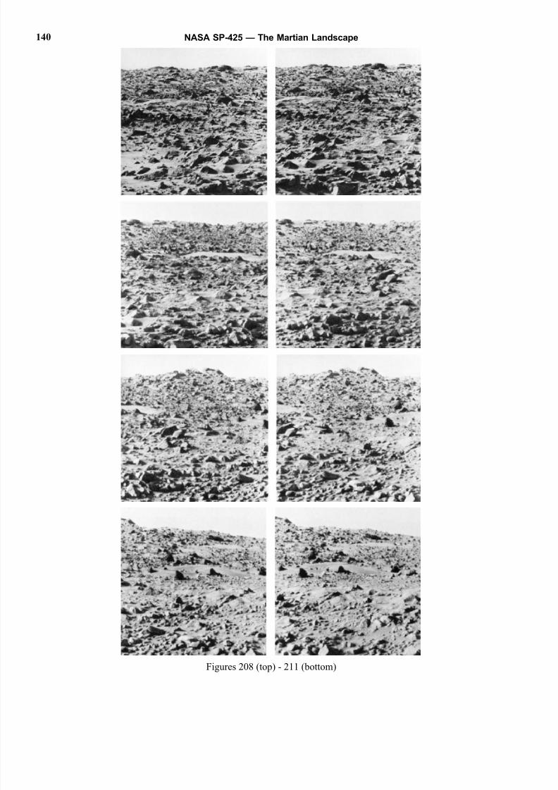
8/8/2019 The Martian Landscape
http://slidepdf.com/reader/full/the-martian-landscape 140/160
NASA SP-425 — The Martian Landscape140
Figures 208 (top) - 211 (bottom)
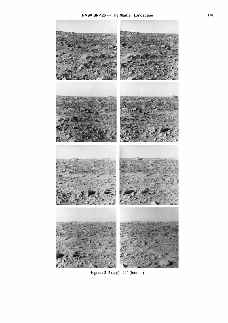
8/8/2019 The Martian Landscape
http://slidepdf.com/reader/full/the-martian-landscape 141/160
NASA SP-425 — The Martian Landscape 141
Figures 212 (top) - 215 (bottom)
8/8/2019 The Martian Landscape
http://slidepdf.com/reader/full/the-martian-landscape 142/160
NASA SP-425 — The Martian Landscape142
Figures 216 (top) - 219 (bottom)
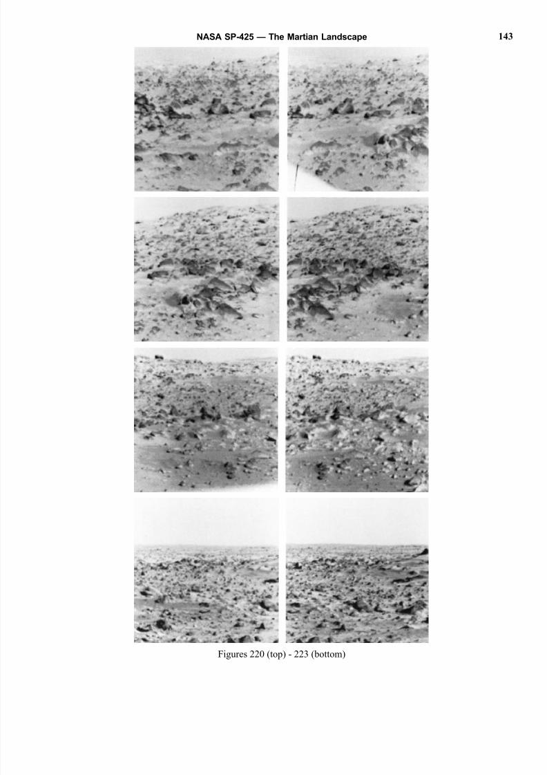
8/8/2019 The Martian Landscape
http://slidepdf.com/reader/full/the-martian-landscape 143/160
NASA SP-425 — The Martian Landscape 143
Figures 220 (top) - 223 (bottom)
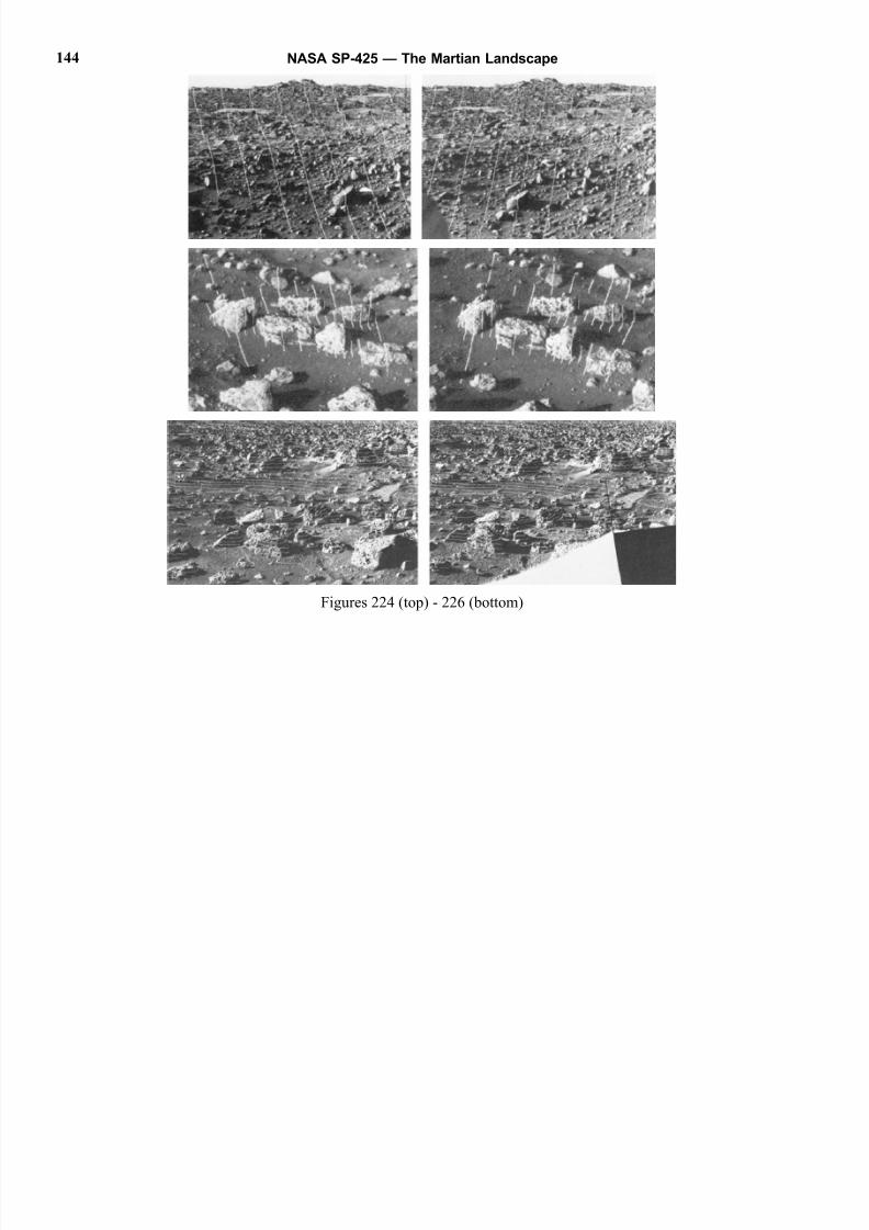
8/8/2019 The Martian Landscape
http://slidepdf.com/reader/full/the-martian-landscape 144/160
NASA SP-425 — The Martian Landscape144
Figures 224 (top) - 226 (bottom)
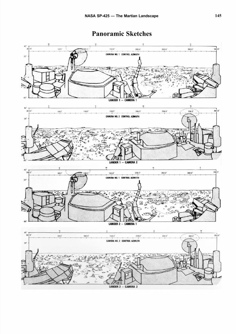
8/8/2019 The Martian Landscape
http://slidepdf.com/reader/full/the-martian-landscape 145/160
Panoramic Sketches
NASA SP-425 — The Martian Landscape 145

8/8/2019 The Martian Landscape
http://slidepdf.com/reader/full/the-martian-landscape 146/160
A Picture Catalog
This table is included for readers who wish to know the “camera settings” for particular pictures. The figure number
in column 1 is followed by the camera event label in column 2. The first number in the camera event label indicates
the Lander and the second number indicates the camera. The letter followed by three numbers indicates the picturenumber, indexed successively starting with the first picture after touchdown. The A series extends from A001 to A255
and is followed by the B series. Accordingly, the camera event immediately following A255 is B000. The first picture
taken after touchdown on July 20, 1976, is labeled 12A001, indicating Lander 1, camera 2, series A, camera event 001.
Azimuth start and stop angles indicate the limits of the published figures. In many cases the total image corresponding
to the camera event has been cropped. The camera control azimuths on the panoramic sketches (see preceding page)
indicate the relative positions of particular azimuths. Also shown are compass directions relative to north.
Lower and upper elevation limits also refer to the published figures, and not necessarily to the limits in the original
images. Refer to the accompanying skyline drawings for the relative positions of particular elevation angles.
Diode selections include low resolution black and white survey (SURV), color (CLR) which is actually a combinationof blue, green, and red diodes, individual color diodes reproduced in black and white labeled BLU, GRN, or RED, Sun,
and high resolution black and white (BB). In the latter there are four focus settings – 1, 2, 3, and 4 – corresponding
to ranges of 1.9, 2.7, 4.5, and 13.3 m.
The significance of gain and offset is described in the introductory text. Most pictures were taken with a gain of 4 and
an offset of 1, camera settings appropriate for scenes with relatively high light levels and considerable contrast.
Greenwich Mean Time (GMT) indicates the time (day, hour, minute) that the picture was taken, measured at
Greenwich, England. Measurements at this locality are the basis of standard time throughout the world.
Local Lander time (LLT) indicates the time that the picture was taken, measured in terms of a Martian system. The
first three numbers refer to the Martian day, or sol, starting with the day of landing, sol 000. This is followed by the
hour and minute, measured after local Martian midnight. Lander 2 sols are not the same as Lander 1 sols, the former
being offset in time because of a later landing.
The Sun azimuth at the time the picture was taken is measured clockwise from north, and the Sun elevation is measured
above the local nominal horizon.
NASA SP-425 — The Martian Landscape146

8/8/2019 The Martian Landscape
http://slidepdf.com/reader/full/the-martian-landscape 147/160
NASA SP-425 — The Martian Landscape 147

8/8/2019 The Martian Landscape
http://slidepdf.com/reader/full/the-martian-landscape 148/160
NASA SP-425 — The Martian Landscape148

8/8/2019 The Martian Landscape
http://slidepdf.com/reader/full/the-martian-landscape 149/160
NASA SP-425 — The Martian Landscape 149

8/8/2019 The Martian Landscape
http://slidepdf.com/reader/full/the-martian-landscape 150/160
NASA SP-425 — The Martian Landscape150

8/8/2019 The Martian Landscape
http://slidepdf.com/reader/full/the-martian-landscape 151/160
NASA SP-425 — The Martian Landscape 151
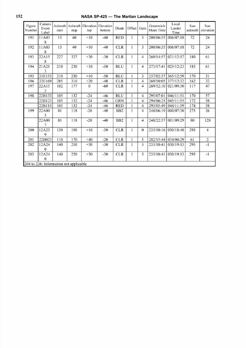
8/8/2019 The Martian Landscape
http://slidepdf.com/reader/full/the-martian-landscape 152/160
NASA SP-425 — The Martian Landscape152

8/8/2019 The Martian Landscape
http://slidepdf.com/reader/full/the-martian-landscape 153/160
The Authors
The success of the Viking mission represents the contributions of many thousands of persons whose signatures are
contained in a microdot attached to each of the Viking Landers. Also, many people contributed directly to the Lander
Camera Investigation. Some participated in the design and construction of cameras. Others planned the imaging
sequences during the mission. Still others processed the imaging data returned to Earth. All should be identified as
coauthors of this volume.
Some of these persons are identified below, according to their functional position. We say some because no listing
however long, is complete. In balance, we felt it more appropriate to list persons by name rather than to take refuge
in the more common generalized acknowledgment to “all those who made this possible.”
Thomas A. Mutch
Kenneth L. Jones
NASA SP-425 — The Martian Landscape 153
Viking Project Administrators
James S. Martin, Jr.
NASA Langley Research Center
Project Manager
Israel Taback
NASA Langley Research Center
Deputy Project Manager (Technical)
Gerald A. Soffen
NASA Langley Research Center
Project Scientist
A. Thomas Young
NASA Langley Research Center
Mission Director
G. Calvin Broome
NASA Langley Research Center
Lander Science Instruments Manager
Lander Imaging Science Team
Thomas A. Mutch
Brown UniversityTeam Leader
Elliott C. Levinthal
Stanford University
Deputy Team Leader
Glenn R. Taylor
NASA Langley Research Center
Assistant Team Leader
William R. Patterson
Brown UniversityTeam Engineer
Alan B. Binder
University of Kiel
Friedrich O. Huck
NASA Langley Research Center
Sidney Liebes, Jr.
Stanford University
Elliot C. MorrisU.S. Geological Survey
James B. Pollack
NASA Ames Research Center
Carl Sagan
Cornell University
Andrew T. Young
Texas A. & M. University
Lander Imaging Flight Team
All members of the Science Team plus the following:
Raymond E. Arvidson
Washington University
Also Science Team Leader, Extended Mission
Philip Avrin
Martin Marietta

8/8/2019 The Martian Landscape
http://slidepdf.com/reader/full/the-martian-landscape 154/160
C. Ernest Carlston
Martin Marietta
Robert D. Collie
NASA Langley Research Center
Paul Fox
Cornell University
Sven U. Grenander
Brown University
Kenneth L. Jones
Brown University
Carroll W. Rowland
NASA Langley Research Center
R. Stephen Saunders
Jet Propulsion Laboratory
Robert B. Tucker
Stanford University
Stephen D. Wall
NASA Langley Research Center
Michael R. Wolf
Jet Propulsion Laboratory
Camera Design, Construction, and Testing
Charles H. Ross
ITEK
Manager, camera construction program
Gerald Amante
EGG Incorp., Bedford Div.
Photosensor array fabrication
Antony Aponik
EGG Incorp., Bedford Div.
Photosensor array fabrication
Raymond P. Babcock
ITEK
Camera construction, Optical Alignment and Test
Equipment Engineer
Clarence J. Biggar
ITEK
Camera construction, electrical assembly
NASA SP-425 — The Martian Landscape154
Michael D. Borenstein
Martin Marietta
Photosensor assembly, system level test
Troy G. Brooks
NASA Langley Research Center
Photosensor fabrication
John D. Buckley
NASA Langley Research Center
Photosensor fabrication
Ernest E. Burcher
NASA Langley Research Center
Facsimile camera design
Raymond J. Capobianco
ITEK
Camera construction, system quality assurance
Stephen L. Carman
Martin Marietta
Lander level camera testing
Vincent H. Corbett
Martin Marietta
ITEK Resident Team Manager
Parker J. Crossley
ITEK
Camera construction, program configuration
Billy B. Dancy
NASA Langley Research Center
Photosensor fabrication
William J. Davis
ITEK
Camera construction, Optical System Engineer
Donald K. Dean
Martin Marietta
ITEK Resident Team, quality assurance
Douglas P. Diederich
Martin Marietta
Camera testing
Roy A. Deveau
ITEK
Camera construction, Design Draftsman

8/8/2019 The Martian Landscape
http://slidepdf.com/reader/full/the-martian-landscape 155/160
Jules Dishler
Martin Marietta
Camera system requirements definition
John J. Donahue, Jr.
ITEK
Camera construction, systems engineering and Science
Team liaison
Herbert W. Feinstein
ITEK
Camera construction, Staff Engineer for elevation axis –
mechanical design
Joseph J. Fiorilla
ITEK
Camera construction, Program Chief Engineer
John C. Fleming
Martin Marietta
Photosensor assembly, filter design and testing
Kim B. Franzoni
ITEK
Camera construction, Contract Administrator
Robert N. Fuller, Jr.
ITEK
Camera construction, elevation and azimuth control
system development
John W. Gerdes
ITEK
Camera construction, Tiger Team Program Manager
Norman S. Goralnick
ITEK
Camera construction, Development Engineer
Ray D. Harrell
Martin Marietta
Photosensor assembly, configuration management
Morriss L. Holliday
NASA Langley Research Center
Photosensor fabrication
Frederick H. Hudoff
Martin Marietta
Photosensor assembly, Program Manager
NASA SP-425 — The Martian Landscape 155
Kenneth L. Jacobs
NASA Langley Research Center
Consultant, servo design
Daniel J. Jobson
NASA Langley Research Center
Facsimile camera design
Michael Kardos
Martin Marietta
ITEK Resident Team, Product Integrity Engineer
Stephen J. Katzberg
NASA Langley Research Center
Facsimile camera design
W. Lane Kelly IV
NASA Langley Research Center
Facsimile camera design
Melvin W. Kuethe
Martin Marietta
Dust protection design and testing
Jules J. Lambiotte, Jr.
NASA Langley Research Center
Facsimile camera design
Frank L. Lawrence
NASA Langley Research Center
Photosensor fabrication
Lawrence Leonard
EGG Incorp., Bedford Div.
Photosensor array fabrication
William F. Loughlin
ITEK
Camera construction, electronics assembly integration
Samuel C. Lukes
Martin Marietta
CO2 dust removal, Program Manager
Thomas K. Lusby, Jr.
NASA Langley Research Center
Photosensor fabrication
Allan J. MacEachern
ITEK
Camera construction, Tiger Team Chief Planner

8/8/2019 The Martian Landscape
http://slidepdf.com/reader/full/the-martian-landscape 156/160
James W. MacFarlane
ITEK
Ground reconstruction equipment, Project Engineer
Clifford J. Maxwell
ITEK
Ground reconstruction equipment
Henry F. McCall
ITEK
Camera construction, Electronics Lead Engineer
John H. Montgomery
Martin Marietta
Camera electronic design analysis
Raymond Peluso
Martin Marietta
Photosensor array fabrication
Robert B. Penninger
ITEK
Ground reconstruction equipment, Program Engineer
Albert R. Philips
NASA Langley Research Center
Photosensor fabrication
John J. Rezendes
ITEK
Camera construction, program production control
James H. Rich
ITEK
Camera construction, mechanical manufacture,
Technical-Specialist
Kenneth H. Schlichtemeier
Martin Marietta
Camera electronics, worst case analysis
Rennald C. Schmidt
Martin MariettaPhotosensor assembly, quality control
Eric Schwarm
Martin Marietta
Camera servo design analysis
Donald A. Stang
Martin Marietta
Dust protection device, fabrication
NASA SP-425 — The Martian Landscape156
Staulo Salvatore
ITEK
Camera construction, Chief Mechanical Engineer
Lyman A. Stilley, Jr.
NASA Langley Research Center
Photosensor fabrication
David Stout
Martin Marietta
Preliminary camera electronics design
Rush B. Studinski
Martin Marietta
ITEK Resident Team, Subcontract Administrator
Eugene R. Sullivan
ITEK
Camera construction, Program Administrator
Rowland Tully
NASA Langley Research Center
Photosensor fabrication
Donald L. Tushin
ITEK
Camera construction, component and system testing
Doris M. Tyler
ITEK
Camera construction, printed circuit card assembly
John G. Waring
Martin Marietta
Field test electronic design
Maywood L. Wilson
NASA Langley Research Center
Photosensor fabrication
Virgil F. Young
Martin Marietta
Photosensor assembly, circuit design
Image Formatting and Processing
Kermit S. Watkins
Jet Propulsion Laboratory
Manager, image processing system development
David L. Atwood
Jet Propulsion Laboratory
Calibration data processing

8/8/2019 The Martian Landscape
http://slidepdf.com/reader/full/the-martian-landscape 157/160
William J. Beckmann
Jet Propulsion Laboratory
Photolaboratory technician
William D. Benton
Jet Propulsion Laboratory
Color image reconstruction
Joseph W. Berry
Jet Propulsion Laboratory
Geometric rectification software, computer mosaics
D. Thomas Box
Jet Propulsion Laboratory
Supervisor, Mission and Test Photosystem
Roger Brandt
Jet Propulsion Laboratory
Computer hardware configuration and maintenance
William J. Chandler
Jet Propulsion Laboratory
Mission and Test Photosystem Engineer
Charles E. Frasier
Jet Propulsion Laboratory
First order image processing software
Joseph Fulton
Jet Propulsion Laboratory
Computer hardware configuration and maintenance
Joseph D. Gaunder
Jet Propulsion Laboratory
First order image processing
Michael A. Girard
Jet Propulsion Laboratory
Interactive image processing system software
William B. Green
Jet Propulsion Laboratory
Leader, image processing staff
Lawrence S. Green
Jet Propulsion Laboratory
First order image processing software
William Harlow
Stanford University
Stereo station construction
NASA SP-425 — The Martian Landscape 157
Paul Harari
Jet Propulsion Laboratory
First order image processing
John C. Hewitt
Jet Propulsion Laboratory
Supervisor, photolaboratory
Paul L. Jepson
Jet Propulsion Laboratory
Interactive image display system software
Ralph A. Johansen
Jet Propulsion Laboratory
Supervisor, Mission and test imaging system
Raymond Jordan
U.S. Geological Survey
Stereoplotter
Susan K. LaVoie
Jet Propulsion Laboratory
Team data record processing, computer mosaics
Edward Y. S. Lee
Jet Propulsion Laboratory
Interactive picture catalog system
Fred H. Lesh
Jet Propulsion Laboratory
System Programmer
Jean J. Lorre
Jet Propulsion Laboratory
Radiometric decalibration software
Donald J. Lynn
Jet Propulsion Laboratory
Deputy Leader, image processing staff
Michael D. Martin
Jet Propulsion Laboratory
Photoproduct storage and distribution system
Mary G. McGough
Jet Propulsion Laboratory
Photolaboratory Technician
Edward Morita
Jet Propulsion Laboratory
First order image processing

8/8/2019 The Martian Landscape
http://slidepdf.com/reader/full/the-martian-landscape 158/160
Duane K. Patterson
Jet Propulsion Laboratory
Photolaboratory Technician
Rodger N. Philips
Jet Propulsion Laboratory
Data logging, graphics display software
Robert W. Post
Jet Propulsion Laboratory
Photolaboratory Technician
Margaret A. Power
Jet Propulsion Laboratory
Stereopair processing and projection software
Gerald A. Praver
Jet Propulsion Laboratory
Manager, Mission and test photosystem
Lynn Quam
Stanford University
Image processing software
Arnold A. Schwartz
Jet Propulsion Laboratory
Lander stereophotogrammetry analysis and software
Joel B. Seidman
Jet Propulsion Laboratory
Supervisor, Image Processing Laboratory OperationsGroup
Ted Sesplaukis
Jet Propulsion Laboratory
Automated image cataloguing
Steven Silverman
Jet Propulsion Laboratory
Computer hardware configuration and maintenance
Deborah M. Spurlock
Jet Propulsion LaboratoryExperiment data record production
Norma J. Stetzel
Jet Propulsion Laboratory
Mission and Test Photosystem Quality Control Engineer
V. W. Tuk
Jet Propulsion Laboratory
Computer hardware configuration and maintenance
NASA SP-425 — The Martian Landscape158
Jurrie J. Van der Woude
Jet Propulsion Laboratory
Photolaboratory Group Leader
Ronald J. Wichelman
Jet Propulsion Laboratory
Photographic engineer
Jackson Wilson
Jet Propulsion Laboratory
Automated image cataloguing
Sherman S. C. Wu
U.S. Geological Survey
Photogrammetry
Mission Planning
Kayland Z. Bradford
Martin Marietta
Image sequence simulation
Elizabeth F. Buchan
NASA Langley Research Center
Image sequencing
Carolyn G. Cooley
Martin Marietta
Image sequence planning
William C. Eggemeyer Washington University
Image sequencing
R. Terry Gamber
Martin Marietta
Image sequence planning
Lloyd E. Gilbert
Martin Marietta
Imaging software development
James GliozziMartin Marietta
Sample site imaging coordination
Jaryl K. Kerekes
Martin Marietta
Image sequencing
B. Gentry Lee
Martin Marietta
Director, Science Analysis and Mission Planning

8/8/2019 The Martian Landscape
http://slidepdf.com/reader/full/the-martian-landscape 159/160
Donald W. Marquet
Martin Marietta
Mission event sequence planning
Deborah G. Pidek
Martin Marietta
Image sequencing
James D. Porter
Martin Marietta
Mission event sequence planning
Albert R. Schallenmuller
Martin Marietta
Mission software development and integration
Janet A. Shields
Martin Marietta
Image sequencing
Henry C. Von Struve III
Martin Marietta
Lander science planning
Edward J. Taylor
General Electric Corporation
Imaging planning and software development
Hugh N. Zeiner
Martin MariettaImage sequence planning
Adjunct Science Analysts
Edward W. Dunham
Cornell University
Edward A. Guinness
Washington University
Bruce W. Hapke
University of Pittsburgh
James W. Head 111
Brown University
Ralph A. Kahn
Harvard University
Baerbel K. Lucchitta
U.S. Geological Survey
NASA SP-425 — The Martian Landscape 159
Dag Nummedal
University of South Carolina
David C. Pieri
Cornell University
James R. Underwood, Jr.
Kansas State University
Support Personnel
Sarah H. Bosworth
Brown University
Secretary
Richard E. D’Alli
Brown University
Viking Intern Program Administrator
Leslie A. Lloyd
Jet Propulsion Laboratory
Photolibrarian
F. Wayne Loer
NASA Langley Research Center
Secretary
Madeline M. Mutch
Providence, R.l.
Sustainer
Charlotte M. Scherig
ITEK
Secretary
Viking InternsUndergraduates selected by national competition to
participate in mission operations
Richard O. Ackermann
California Institute of Technology
Steven Albers
Muhlenberg College
Kenneth G. Carpenter
Wesleyan University
Andrew L. Chaikin
Brown University
Eric H. Christiansen
Brigham Young University

8/8/2019 The Martian Landscape
http://slidepdf.com/reader/full/the-martian-landscape 160/160
R. Glenn Cooper
Rice University
Mark A. Croom
Virginia Polytechnic Institute
William E. Dieterle
Arizona State University
Mark B. DuBois
Harvard University
Chris Eberspacher
University of Texas
F. Donald Eckelmann, Jr.
Colgate University
Mark I. Heiligman
Amherst College
Edward A. Hildum
Massachusetts Institute of Technology
Albert R. Hochevar
U.S. Naval Academy
NASA SP-425 — The Martian Landscape160
Julio Magalhaes
Stanford University
William B. McKinnon
Massachusetts Institute of Technology
Kurt D. Molenaar
Macalester College
Barbara A. Murphy
Lehigh University
John J. Polcari
U.S. Naval Academy
David W. Thompson
Massachusetts Institute of Technology
Judy C. Thompson
Massachusetts Institute of Technology
Michael C. Wright
University of Tennessee