The macro-micro paradox of

aid and volatility

Investigating the macro- and microeconomic

effects of aid

Author: T. Arkes, 403087

Supervisor: E.M. Bosker

Master thesis

Erasmus University Rotterdam, Erasmus School of Economics

MSc Economics and Business, International Economics

Abstract:

This thesis investigates the efficiency of aid to see whether aid has an effect on the

economic performance of a recipient country. Scholars have over the years found that aid

flows do not have an effect on a recipient‟s macroeconomic performance. This research

replicates those results.However, this research finds that on the microeconomic level aid

flows do have an effect on the death rate and mobile phone and internet subscriptions. There

is thus a macro-micro paradox of aid. Furthermore, aid volatility is found to have a negative

effect on both macroeconomic and microeconomic performance of a recipient. The effect on

the macroeconomic level is dependent on whether a country is aid dependent or not.

Geographical location is also determining factor. On the microeconomic level aid volatility

has a negative effect, even when volatility is a positive deviation from the aid trend.

1

Contents 1. Introduction .................................................................................................................................... 2

2. Literature review ........................................................................................................................... 3

2.1 Aid-growth efficiency ............................................................................................................. 3

2.2 Aid conditionality .................................................................................................................... 5

2.3 Aid volatility ............................................................................................................................. 6

2.4 Aid predictability ..................................................................................................................... 8

2.5 Relevance of this research ................................................................................................... 9

3. Methodology ................................................................................................................................ 10

3.1 Model specifications ............................................................................................................ 10

3.2 Measuring volatility .............................................................................................................. 12

3.3 Measuring aid predictability ................................................................................................ 12

3.4 Estimation methods ............................................................................................................. 13

4. Data description .......................................................................................................................... 13

4.1 Dataset................................................................................................................................... 13

4.2 Total aid flows ....................................................................................................................... 13

4.3 Sector aid flows .................................................................................................................... 15

4.4 Aid volatility ........................................................................................................................... 19

4.5 Trends in aid volatility .......................................................................................................... 21

5. Empirical macroeconomic analysis and results ..................................................................... 24

5.1 First look at aid, volatility and predictability ...................................................................... 24

5.2 Following Hudson and Mosley ........................................................................................... 25

5.3 The effects of aid based on recipient characteristics ..................................................... 26

5.4 The effect of aid predictability ............................................................................................ 28

5.5 Statistical problems with models ........................................................................................ 29

5.6 Summary ............................................................................................................................... 30

6. Empirical microeconomic analysis and results ...................................................................... 30

6.1 General models .................................................................................................................... 30

6.2 Following Hudson ................................................................................................................. 32

6.3 Macro-micro paradox ........................................................................................................... 33

7. Conclusion and discussion ....................................................................................................... 34

8. Reference list .............................................................................................................................. 36

Appendix .......................................................................................................................................... 38

2

1. Introduction

This research places the aid efficiency debate into a new timeframe: the twenty-first century.

This is partly done because of the availability of superior data with regards to not only aid

flows but also data on other economic indicators. Furthermore, research has predominately

used data of the previous century whereas this research uses only the years 2002-2013

thereby looking at the contemporary effects of aid and volatility.

Donor attitude towards aid has been changing very much over the past 40 years and

problems that aid had in the past with regards to efficiency might very well not be relevant in

current time. Furthermore, certain trends of aid would not be adequately visible when the last

12 years of aid would not have been the focus. This research finds that total aid flows have

been increasing over the last 12 years. Aid as a percentage of GDP, on the other hand, has

seen a decreasing trend since the year 2006. This is also the case for aid volatility. These

trends were also found by Hudson (2014) and could lead to the assumption that there is a

diminishing effect of both aid and its volatility on a recipient‟s economy. In investigating this

relation, it is found that in itself aid and volatility do not significantly affect macroeconomic

performance, as measured by the GDP per capita growth rate. Also, following previous

research but changing the time period leads to the effects of aid flows and volatility on the

GDP per capita growth rate not being statistically significantly anymore. Adding interaction

terms of aid volatility and country characteristics changes the outcomes found previously and

leads to significant results. With the addition of an interaction term for aid dependency (>10%

of GDP as aid flow), volatility of aid disbursements has a negative effect on the GDP per

capita growth rate of countries that are not aid dependend. For aid dependend countries this

effect is very small and positive which may be a sign of reverse causality. Similar results are

found when adding interaction terms for Sub Saharan Africa. For countries in South America,

disbursement volatility has a negative effect on GDP per capita growth. The effect of aid

predictability, measured by the difference between commitments in t-1 and disbursements in

period t, on macroeconomic performance is also investigated. This measure gives, when

significant, a negative coefficient indicating a reverse causality problem. This indicates that

the difference between commitments and disbursements in itself is of no importance to

recipient countries.

The focus is then shifted towards investigating whether the absence of significant impacts of

aid and aid volatility on the entire dataset is due to the macro-micro paradox, indicating that

macroeconomic indicators are not affected but microeconomic performance of a recipient is.

Following Hudson (2014) this research finds that for all countries in the dataset and for

certain microeconomic indicators and aid sectors, aid flows still have significant effects.

These effects, depending on the indicator, are both positive and negative. Furthermore,

volatility is also important in influencing microeconomic performance of a recipient. It is found

that volatility in the form of positive deviations from the trend (positive volatility) can have a

negative effect. To conclude, this research thus finds for the macroeconomic level various

results with regards to significance, but is able to find negative effects of aid volatility on GDP

per capita growth rate. The significance of aid flows at the microeconomic level shows that

with regards to just the aid flows there seems to be a micro-macro paradox. With regards to

volatility, this seems to be a problem (with negative effects) on both the macro- and

microeconomic level.

Section 2 below contains a literature review that briefly discusses literature on the aid

effectiveness debate, aid conditionality, aid volatility and aid predictability. Section 3 presents

3

the methodology and discusses the models used for this research and how volatility and

predictability are measured. Section 4 is an elaborate data description that contains

information on aid flows and aid volatility and their respective trends. Sections 5 and 6

discuss the results of the models that are shown by section 3 for the macroeconomic and

microeconomic analyses respectively. Section 7 contains a summary of the results and ties

these together with a conclusion.

2. Literature review

The aid effectiveness debate contains vast amounts of literature spanning over multiple

decades. As is the case with most economic literature, findings and opinions change over the

years. Below is a summary of the most important and influential literature on the subject.

2.1 Aid-growth efficiency

Earlier research has long focused on only short-term performance of aid. Only relatively

recently have scholars taken it upon themselves to test the long-term macroeconomic effects

of aid flows for the recipient country. When taken in its simplest form, aid is no more than a

government lump-sum transfer. The aid efficiency debate can therefore be traced back to the

days of Keynes (1929) who investigated the so-called transfer problem. The transfer

problem covered the transfer of capital between two stable economies in a two-country world

in the form of unrestricted gifts from one government to another. In the end, these capital

transfers impoverished to donor and enriched the recipient of the capital. Terms of trade,

however, were affected, giving a possible reason for these capital transfers. Modern-day

research done on the transfer problems steps away from the two-country model and adds

more countries. This addition of more countries can actually reverse the welfare effects,

where welfare increases due to transferring capital to another economy. Welfare in the

recipient country is actually decreased, causing the so-called transfer paradox. The transfer-

paradox as described by Gale (1974) explains that if a (industrialized) donor country has a

very specific demand and strong preference for a certain good, a transfer is able to reduce

the worldwide demand and cause excess supply for that good thereby reducing its prices.

This then means that for the industrialized donor country the real income rises (which can be

seen as a gain in welfare). The reduced prices, on the other hand, cause the income of the

recipient country to decrease. The size of the transfer could offset this, but in the long run

prices will be lower than before, thereby decreasing welfare. As Gale (1974) argues, when

agents scheme together versus the rest of the world, this can cause a welfare decrease for

the rest of the world, while both agents (donor and recipient) gain from the transfer due to

decreased prices of imports as well as an increase in wealth for the recipient. To summarize,

according to literature up to the year 1973 lump-sum transfers can have both negative and

positive effects for every agent involved, whether it be the recipient, the donor or even the

rest of the world involved in any sort of trade with either agents. This shows that the transfer

of capital from one country to another and the effect thereof is, in theory, not without its

discussions and contradictions.

When aid is no longer a „pure‟ transfer in that it is not just a lump-sum transfer but directed

aid towards public investment („productive‟ transfer), it is found that aid will stimulate the

steady-state growth of the recipient country, whereas a „pure‟ transfer will not affect the

steady-state growth. However, welfare is increased due to an increase in consumption

caused by the transfer (Chatterjee et al., 2003). In the long-run, an increased steady-state

growth has a potentially larger positive effect, even though the instantaneous effect on

welfare is smaller. However, this steady-state growth is not always given as it depends on

4

how well the recipient country is endowed with public capital. The positive effects are seen in

relatively under-endowed economies, whereas well-endowed economies can even show

decreases in growth (Chatterjee et al., 2003). Because developing countries are generally

under-endowed when it comes to public capital, it would seem that when aid is „productive‟ in

that it is aimed towards increasing public capital and public investment, aid should have a

positive effect on welfare as well as (steady-state) economic growth.

Empirically, literature on the matter has been far from unanimous, finding both significantly

positive and negative effects of aid. Clemens et al. (2004), Mosley (1980) and Hansen &

Tarp (2000) identify different phases of literature, covering different time periods and

methods on measuring aid effectiveness. Research done by Griffin (1970) investigates the

relation between the inflow of foreign capital (more than just aid) and investment levels. He

argues there is a possibility that the small positive effect that the inflow of foreign capital has

on domestic investment will be countered by the diminishing effect it has on capital-output

ratio, causing the growth rate to drop. This is later confirmed by Weisskopf (1972) who finds

a negative relation between foreign capital inflows and domestic savings.

The subsequent literature actually looks at aid, instead of general inflows of foreign capital.

Because of the distinction between aid and general foreign capital, Panapek (1973) now

finds a positive and significant effect of aid on growth. Methods of research however, do not

look at causality and do not use instruments. For example, Panapek (1973) is not able to find

significant effects of aid on growth when he restricts his data to just North- and South-

America. Furthermore, research is mainly done on small 5-year periods, neglecting any long-

term effects aid could have on growth.

Mosley (1980) then questions the causality of the previously found relationships between aid

and growth. What follows is roughly 15 years of literature that empirically researches the

relations of aid and growth by using different countries, periods and instruments. This leads

to very contradictory literature. Scholars find significant positive effects (Levy, 1988) as well

as no significant effects (Mosley et al. 1987, Singh, 1985). This „era‟ of literature finishes with

Boone (1996) who uses a large dataset which also controls for country fixed effects. With

these country fixed effects he finds zero correlation, whereas without the country fixed effects

there is a positive coefficient, albeit only at the 10% significance level. As stated before,

research up until this point used small periods of time, only looking at short-term effects of

aid. As Clemens et al. (2004) argue, Boone‟s (1996) research rejects the hypothesis of zero

or negative effect at the 5% level when the time-period is extended to 10 years. According to

Clemens et al. (2004) it is Boone‟s research that spurred the last phase of the aid-growth

literature. Following Boone, some scholars conclude that there is a macro-micro paradox of

aid: aid has positive economic effects on the microeconomic-level which somehow is not

observable on the macroeconomic-level. In this next phase, literature is divided in research

that addresses this paradox, and research that does not.

As was the case with the previous phase, the most recent literature does not produce

unanimous results either. This is also due to the above-mentioned divide in the literature

itself. The „conditional‟ literature says that on average aid in itself has zero effect on growth.

Countries that do seem to get a positive effect of aid on growth have certain characteristics

which makes the aid effective. The conditional literature is aimed towards identifying these

characteristics. This does not lead to one answer either, and over the years various

characteristics have been found that are argued (both theoretically as empirically) to be

5

necessary for economic growth through aid. Because this part of literature looks at why the

typical country that receives aid is not able to turn that aid into something positive, this strand

of literature has been very influential in policy-making.

The „unconditional‟ literature, on the other hand, still argues that aid in itself has, on average,

a positive effect on economic growth. This strand of literature is therefore more aimed

towards the investigation of the relation between aid and growth, and whether it is linear or

non-linear. This strand of literature also contains research that finds a positive effect of aid,

regardless of a non-linear effect.

2.2 Aid conditionality

As mentioned above, literature and aid-donor countries have recently shifted their focus on

conditions that a recipient country has to fulfill in order to obtain certain ODA-funds. These

conditions originante from the idea that a simple lump-sum transfer has no economic effect if

the right conditions are not present in the recipient country. Traditionally donor-countries

made commitments of aid-transfers and then, when due, transferred these committed funds

to the recipient country in the form of an aid disbursement. Conditions of aid formed when

the goals of aid became more specified. Over the years, aid-donors have made multiple

agreements on the focus of aid, for example the millennium goals, whose aim was to

decrease the amount of people living beneath the poverty line of $1 per day and in hunger to

half of the amount in 1990 (Temple, 2010). This is, as is also argued with the macro-micro

paradox, not done by simply transferring large funds to problem areas and assuming that

poverty and hunger will thereby decrease. Donors therefore have to focus on improving

microeconomic mechanisms to be able to affect the economy on the macroeconomic level.

Conditionality of transfers began in the 1980‟s when the IMF and World Bank started

disbursing aid when certain conditions were met by the recipient country with regards to

wider policy reforms and macro-economic performance of the recipient (Temple, 2010).This

basic conditionality of aid has been widely investigated and discussed and has been

generally seen as ineffective and counter-productive in literature (Temple, 2010, Easterly,

2005). The ineffectiveness of aid conditionality can come from multiple mechanisms that

exist within a donor-recipient relationship. As is the case with these types of transfers, there

exists a principal-agent problem. A donor may have different goals than the recipient country

with regards to certain policies other than the main focus of the aid. For example aid can be

used to decrease poverty which is the main goal of the aid disbursement. As a secondary

goal, the donor can demand of the recipient country to implement other policy reforms that

do not necessarily have anything to do with the reduction of poverty. In a way a donor

country tries to buy another reform within the recipient country which probably would not

have happened without the promise of an aid disbursement. This can then also mean that

whenever aid is disbursed the secondary policy reform can be reversed as it is not in the

interest of the agent to keep it. Strong conditionality can keep this from happening because

reversing reform will mean a reduction in aid disbursements in the following periods. In

theory this is an effective way of reforming the policies of an aid-dependent country towards

a more sophisticated way of governing. Literature, however, has found that this classic type

of conditionality of aid has led to very little improvements of macroeconomic policies in

developing countries. Furthermore, countries that are aid-dependent are not among the most

stable countries in the world with regards to governments. They vary from dictatorships to

countries with high corruption levels and so reforms are very hard to implement in these

countries. This then means that a lack of condition enforcement by a donor leads to the

6

recipient receiving disbursements regardless of policy reform. Furthermore, donor countries

may not be influential enough to sway a government towards reforming policies that are not

of interest to them. Volatility in aid flows has, due to these conditions, the potential to make

aid-commitments lack credibility within the private sectors (Collier et al., 1997).

Because of the absence of positive results due to policy conditionality, donor countries have

been developing other ways of choosing where and when to disburse aid. Donors can

choose to allocate aid disbursement towards countries in which it is most likely to be effective

and successful. This way of allocating aid, called selective aid allocation, comes back to the

argument that aid can only be successful when certain conditions are met within a recipient

country. Rather than trying to enforce these conditions it is more logical to first help countries

in which these conditions are already met. However, the problem of allocating aid this way is

that the great unknown is what makes aid effective. Literature with regards to aid flows and

aid conditionality have yet to find a uniform answer to whether aid in itself is effective, let

alone which conditions make aid effective. Regardless of it not being clear what makes aid

effective, it can easily be argued that current aid allocation is far from optimal (Collier and

Dollar, 2002). There are many donors, and with unclear allocation optima, disbursements of

aid are rather uncoordinated. As Collier and Dollar (2002) argue, coordinated and systematic

disbursements of aid by donors can potentially double the amount of people that escape

poverty per year.

With regards to reform based conditionality, a more progressive form of conditionality is

being implemented by certain donors which entails that instead of a recipient having to meet

a certain requirement at a certain date, commitments have no end date on which the reforms

will be evaluated (Temple, 2010). This means that whenever a reform is made and thus a

condition is met, aid will be disbursed. This directly means that aid can be disbursed before it

would have traditionally been, but a recipient country can also delay the disbursement by

delaying the reform until a moment that it sees fit. This directly means that predictability of

aid for a recipient country can increase due to its control on when the disbursement will

happen. On the other hand, aid volatility will increase as disbursement will no longer follow a

certain trend.

2.3 Aid volatility

Aid volatility fully entered the aid-efficiency debate when Bulíř & Hamann (2003) investigated

the policy implications of uncertain of aid flows. They found that aid flows are more volatile

than the domestic revenue of a recipient country. Countries that show higher volatility of

revenues also display higher levels of aid volatility. This indicates that both aid flows and

domestic revenues could be influenced by the instability of domestic policy. Furthermore, aid

is found to be procyclical. This follows from donor-countries being unable to check whether

disbursements have been successful, leaving them to tie conditional aid to economic

performance. This then means that any shock in economic performance can lead to highly

inconsistent and unpredictable aid-flows. Aid dependent countries in themselves are more

prone to these shocks in economic performance because of liquidity constraints and bad

policy making. In all its effort to help improve economic policy in developing countries, aid

and its volatility cause the macroeconomic performance of a developing country to be more

unstable. Aid volatility itself can be traced back to both donors and recipients of aid. Donors

often make commitments that are higher than the actual disbursements that follow, this is

also due to the nature of commitments. Commitments are not obligated to follow the same or

next year and are thus not subject to a time-frame. This then means that coupled with aid

7

conditionality, a commitment could in theory take more than a decade to be fully disbursed.

Recipient countries react to these commitments and adjust policy accordingly. Failure of a

donor country to donate that amount of aid in a short enough amount of time can thus leave

a gap in the recipient‟s budget. Furthermore, because of the before mentioned aim to

improve on a recipient‟s economic policies, aid has become highly conditional. Even though

a commitment is made by a donor, failure to meet the right requirements leads to a lower

disbursement for the recipient country. This then also means that when a recipient country is

not able to adjust its policies in the right way, the volatility of its aid inflows

increases.However, aid dependent countries are often dependent on aid because of their

instability and inability to formulate proper economic policy. In their follow up research (Bulíř

& Hamann, 2008)did not find any changes compared to five years prior, even though

literature seems to have shifted a little more of its attention towards aid volatility. Even

though it is now known that aid is volatile, large economic shocks caused by the unstabling

effect of aid volatility are not being countered by aid disbursements (Bulíř & Hamann, 2008).

This then means that aid policy of donors is still not aimed towards undoing any negative

effects of aid volatility. Not through stabilizing aid flows themselves, and not through

countering any negative effects that are caused by unstable aid flows.

Following Bulíř and Hamann (2003) literature has set out to investigate the causes of aid

volatility and also the effects of aid volatility. As mentioned above, these findings did not lead

to any significant policy changes for either donor or recipient. (Arellano, Bulíř, Lane, &

Lipschitz, 2009)look at the effect of aid flows on macroeconomic indicators, as well as the

effect of aid volatility. Increasing aid flows and permanently higher levels of aid do not lead to

increased levels of savings and investments, but do permanently increase levels of

consumption. Aid flows are thus largely transformed into consumption and do not affect

levels of savings or investment on their own. Aid however does increase the rate of return on

capital (Dutch Disease effect) thereby stimulating investment. Increased levels of aid also

show increased levels of influence on economic performance. This means that the higher aid

inflows are, the more dependent the economic performance of the recipient becomes on the

levels of aid, thereby confirming the procyclical nature of aid. Arellano et al. (2009) find a

correlation coefficient of aid and GDP of 0.6, when aid is 20% of GDP as compared to the

coefficient of 0.2 in the benchmark model, where aid is 6.4% of GDP. Because of the large

effect aid has on the consumption, it leads to the conclusion that aid volatility will mainly

affect the consumers, when looking at the welfare effects of aid volatility. Aid volatility is thus

able to create consumption volatility, which is detrimental to welfare. Arellano et al. (2009)

find that when aid flows are stable, aid flows would increase welfare by around 8% of total

aid flows. When aid is given in such a way that, through the right policies, it is able to fully

counter any volatility of consumption welfare levels will increase by around 64% of total aid

flows.

Hudson and Mosley (2008) are the first ones to divide aid volatility in positive and negative

aid volatility. They argue that both have different effects on the shares of GDP to domestic

expenditure. Governments of aid-dependent countries seem to be unable to counter the

negative effects that negative aid volatility has on the revenue flows and expenditure

priorities. Aid volatility thus has a negative effect on investment and even import when it is

negative. Positive aid volatility seems to increase consumption expenditure while also

decreasing the investments and expenditure of governments. This means that governments

lack the absorptive capacity of increased amounts of aid when these increased amounts are

8

not expected. The increase in consumer expenditure shows that consumers are likely to be

better at absorbing both negative and positive shocks through their levels of consumption

and saving (Hudson, 2014). Hudson and Mosley do find that some of the negative impact

positive aid volatility has is later reversed, indicating that the absorptive capacity problems

mentioned before could be short-term only.

Using the Creditor Reporting System (CRS) database, Neanidis & Vervarigos (2009) and

Hudson (2014) look at the impact of aid (volatility) on economic performance divided over

different aid-sectors of purpose (sectors are as defined by the OECD). The first article

divides the sectors over the type of aid, namely pure aid and productive aid. Pure aid is given

in the form of food aid and monetary aid, where it is purely used to be a short term solution to

bad periods (such as bad harvest or flooding). Productive aid on the other hand is divided

over 2 different categories; aid aimed towards improving public services and the physical

infrastructure and aid aimed towards social infrastructure of the economy. Productive aid is

therefore seen as aid that should be effective on the long-run rather than as the short-term

solutions of current pure aid flows. Neanidis and Vervarigos (2009) conclude that productive

aid has a positive impact on economic growth. Volatility of this type of aid, however, has a

negative impact. On the other hand, pure aid transfers do not show positive economic effects

on their own. When pure aid flows are volatile they do seem to have a positive effect on

growth. This contradicts previous findings regarding aid volatility as described above and

therefore indicates there is good reason to distinguish between the different types of aid (with

regards to purpose) to fully capture the effects of aid volatility. Hudson (2014) adds to this by

differentiation aid itself over positive volatility and negative volatility. He finds that increases

in aid volatility, be it negative or positive, are often compensated for in the following period(s)

by fluctuations of volatility in the opposing direction. Furthermore, this compensation in sector

aid volatility seems to cross over to other sectors, mainly governmental aid. The impact

between sectors is mainly negative.

Besides the effects of aid volatility, the causes of aid volatility also differ between total aid

and sector aid. Fielding et al. (2008) find that the volatility of aid is caused by both recipient

and donor countries. Macroeconomic stability of a recipient country is important for total aid

volatility; low inflation decreases total volatility. Conditionality of aid, a much given example

being certain IMF conditions, on the other hand increases total aid volatility. Both these

characteristics, however, have no significant effect on sector aid volatility. Political institutions

significantly influence both total and sector aid volatility. With regards to aid donors only

recipients that receive a high share of aid coming from Arab donors experience higher

volatility.

2.4 Aid predictability

The difference between the aid commitments and aid disbursements of donors can be called

aid predictability (Bullir and Hamann, 2008 & 2003). Aid predictability is, as is argued above,

important for the aid recipient as aid commitments are given some time before the actual

disbursements. With the volatility of the aid itself and the tendency of disbursements to be

lower than commitments, predictability of the amount of disbursements based on

commitments can potentially give a recipient country the chance to fill in the expected deficit

using its own funding. However, aid receiving countries often have crippling liquidity

constraints and will therefore probably not be able to do this on short notice. Failure to

predict aid can thus lead to ineffective allocations of government funds of which there are

already relatively little, which is not desirable. On the other hand, being able to effectively

9

predict aid, not only can a recipient country anticipate budget constraints, it can also

anticipate conditional funds coming in and allocate the incoming disbursements in the most

efficient manner.

Aid predictability is different from aid volatility in that aid volatility, although it is a deviation

from a trend, can be very predictable. Aid commitments can come from large projects taken

on by a donor and can cause a certain influx of aid flows into a recipient country that

significantly deviate from the normal trend in disbursements. This is seen as a positive

volatility. However, since this commitment was already made, in theory it is also predictable.

Aid inflows due to natural disasters or famine are also deviations from that trend, but are on

the other hand not very predictable. The lack of aid predictability can come from either

donors not sticking to their commitments or recipients not sticking to their conditional

requirements.

Celasun and Walliser (2007) investigate the effects of aid predictability and look at whether

the inability of donors to stick to their commitments has any significant effect on a recipient‟s

economy. They find that the stigma that donors do not live up to their commitments is

actually not true in that they find that actual disbursements are both lower and higher than

the commitments that were made. This also leads to another conclusion that, when aid

predictability is caused by both positive and negative deviations from the commitments

made, most countries will suffer from unpredictable aid. Especially budget aid is shown to

have a negative effect when it is unpredictable. If budget aid falls short with more than 1% of

GDP, recipient government have to fill in this gap by accumulating more debt and reducing

capital spending (Celasun and Walliser, 2007). Most destructive of this mechanism is that

these losses in capital spending are not reversed when the shortfall in budget aid is over,

leading the effects of this shortfall to be a permanent one.

2.5 Relevance of this research

Aid volatility research has focused on the aid volatility of the actual aid disbursements, which

makes sense because that is how the actual aid flows are measured. This, however, ignores

the fact that donor countries make commitments towards recipients some time (this can vary)

before sending out the actual aid. It is reasonable to think and often expected that recipient

countries will respond to this through various mechanisms such as political policies. This

research therefore also looks at the difference between the effect of the aid disbursements

and aid commitments. Thus, this research expands on existing literature by looking at both

commitments and disbursements, shifting the period of interest towards more recent years

and by adding aid predictability to aid volatility analysis. Shifting the period of interest gives

an opportunity to see whether trends found by Hudson (2014) in aid volatility have continued

and whether these trends have any influence on the effect of aid volatility. Furthermore, the

focus is also narrowed from country-level data to „aid sector‟-level data and thereby follows

Hudson (2014) in investigating the macro-micro paradox of aid flows and volatility. Lastly, the

effectiveness debate is shifted from all aid receiving countries towards looking at the effects

of aid with regards to certain recipient characteristics. This is done by looking at country

characteristics based on aid dependency (when aid is a certain percentage of GDP) and

region.

10

3. Methodology

3.1 Model specifications

The empirical part of his research is divided over two different sections, with one focusing on

the macroeconomic effects of aid and its volatility (section 5) and the other on the

microeconomic effects of aid and volatility (section 6). The focus on the macroeconomic

effects means that country level data of aid volatility is used instead of aid sector specific

data for aid flows and aid volatility. Furthermore, section 5 looks at macroeconomic specific

dependent and independent variables and thus looks at a more generalized effect. The

section regarding the microeconomic focus uses data on the specific sectors of aid and their

corresponding characteristics as control variables. As these differ between the different

sectors, the dependent variables can also change according to the sector of interest.

This research is based on multiple existing papers. This means that a goal of this research is

to recreate the same models as those papers and if and when possible expand on them.

First, the effects of the independent variables on the dependent variable are tested without

the addition of any other variables in the model. Then, the models that are estimated are

based on existing literature. After that, in the case of the macroeconomic level, an

improvement on that model is used. The models used in this research are as follows:

The most general macroeconomic model:

Where the vector X can be described as the various independent variables that are of

interest in the aid effectiveness literature. These independent variables are the aid flows

themselves, as commitments and disbursements. Also included are the multiple variables for

aid volatility based on both commitments and disbursements. Lastly, the variable of aid

predictability, as described below.

Then, the model used by Hudson and Mosley (2008) is estimated with the addition of year

dummy variables to control for year fixed effects. This model then looks like the following:

The dependent variable, GDP growth, is a measure for economic performance and is the

annual growth rate of GDP per capita in percentages. Descriptions of the independent

variables of interest that involve aid flows are as described in the next section. The variable

GDP per capita is lagged for two periods, as is used by Hudson and Mosley (2008) and

expressed as a logarithm. World growth is the annual growth rate, in percentages, of the

OECD as a total and represents the most important donors of aid and their performance.

Inflation is the lagged value of inflation and thus represents inflation of the previous period.

Inflation is also in percentages and is used as an indicator for government and policy

performance. The disaster variable is a dummy variable which has a value of 1 when the

recipient country is involved in a disaster or famine which affects more than 5% of

population. This data is taken from the EM-DAT database for disasters. Lastly dummy

11

variables are used for different regions. When using fixed effects, however, these dummy

variables are excluded.

Finally, the goal of this research is to go beyond the models described above to see whether

other mechanisms are also at play with regards to aid effectiveness. As mentioned before,

this is done by adding aid predictability and country characteristics to the model. The

macroeconomic model then becomes as follows:

Furthermore, another model is estimated with the addition of aid predictability for every

country and every time period.

The most general microeconomic model is similar to its macroeconomic counterpart:

Where the dependent variables are in this case represented by vector Y, which consists of

different dependent variables based on the aid sector of interest. Vector Y includes for

example death rate, school completion rate and mobile telephone subscriptions. Vector Z, as

did vector X in the macroeconomic model, represents all the different aid variables.

Following Hudson (2014), the final microeconomic models are as follows:

Where total aid flows are the total aid commitments or disbursements. Baseyear value of

dependent variable is the value of the dependent variables used in the year 2002, which is

the starting year for this research.

A summary of the different variables mentioned above and their source are as indicated by

the following table 1:

Table 1: All variables used and their sources

Variable Description Source

GDP per capita growth rate (%) GDP per capita growth

rate as a percentage

WorldBank World

Development Indicators

Aid disbursements Aid disbursements (used

as percentage of

recipient GDP)

OECD CRS database

Aid commitments Aid commitments (used

as percentage of

recipient GDP)

OECD CRS database

GDP per capita Logged value of GDP per

capita

WorldBank World

Development Indicators

World Growth Total GDP of OECD OECD CRS database

12

donor countries

Inflation Inflation as a percentage WorldBank World

Development Indicators

Disaster Dummy variable

indicating disaster in

period for that country

EM-DAT disaster database

Death rate Death rate used as log WorldBank World

Development Indicators

Secondary school completion School completion rate

used as log

WorldBank World

Development Indicators

Mobile phone subscriptions Mobile phone

subscriptions used as log

WorldBank World

Development Indicators

Internet subscriptions Internet subscriptions

used as log

WorldBank World

Development Indicators

Manufacturing value added Value added due to

manufacturing as a

percentage of GDP

WorldBank World

Development Indicators

CO2 emissions CO2 emissions as log WorldBank World

Development Indicators

3.2 Measuring volatility

Measurement of aid volatility has not been uniform over the years and there can therefore be

different choices which all have been proven to give significant results. Most recently Hudson

(2014) has used a self-computed volatility instead of using a Hodrick-Prescott filter (as

argued by Bulíř and Hamann, 2003 and 2008, different measures should give similar results)

and thus this is a logical method to follow for this research. This method of computing aid

volatility entails the regression of aid of a sector on a time trend and its square and then

taking the (squared) deviations from this trend. This leaves, according to Hudson (2014)

room for the aid flows to be both positive and negative, whereas the squared values indicate

the absolute volatility. Volatility is measured for both aid commitments and aid disbursements

over all the relevant sectors. This is done separately for every country, as every country will

have different trends in aid flows. To be able to compare countries and results, aid flows are

taken as a share of recipient GDP. Official development assistance is used for aid flows, this

research thus excludes privately funded aid projects.

3.3 Measuring aid predictability

With regards to aid predictability an assumption has to be made in order to calculate its

value. Aid commitments are not necessarily disbursed in to following period, and can be

made with a longer term. To be able to capture predictability, however, the assumption is

made that an aid commitment is normally set to be disbursed the following year. This then

means that when a commitment is fully disbursed, aid disbursements in period t should equal

aid commitments in period t-1. What follows is that a measure of aid predictability is simply

disbursements in period t, minus the lagged value for commitments.

13

3.4 Estimation methods

This research uses a panel dataset and thus is able to utilize panel model estimation

methods. For completeness, non-panel estimations, random effects estimations and fixed

effects estimations can be found in the appendix for most models. A Hausmann test is used

to see whether fixed effects estimation is a better fit than the random effects estimation.

Depending on these results, the conclusions applicable to that particular model are based on

the best fitting model. This thus means that using fixed or random effects is based on

econometric testing rather than on economic theory. Furthermore, year dummies are added

into the models when they are jointly significant and therefore an improvement on the

models. This is thus also done on the basis of the results of statistical tests.

4. Data description

4.1 Dataset

The dataset used for this research revolves around the Creditor Reporting System (CRS) of

the OECD. The CRS is a system for which donors themselves deliver the data for the

database using elaborate questionnaires. These questionnaires regard both disbursement

and commitments of aid divided over the different „aid sectors‟. These so called aid sectors

are as distinguished by the OECD, which uses the term sector to identify the specific use for

an aid flow. Total aid is thus divided over 10 different sectors which each have their own

respective subsectors. This research focuses only on the 10 largest sectors which will be

described below. Additional data regarding the countries of interest are as provided by the

World Bank organization in their World Development Indicators database as well as the

World Bank‟s Worldwide Governance Indicators and the EM-DAT disaster database.

Countries in the dataset are selected on the availability of data with regards to aid flows in

the CRS database. This means that, at least for total aid flows, every country in the dataset

has a minimum of 2 observations. With regards to additional variables, there is a large

absence of data for certain variables. This vastly decreases the number of countries that are

used in the regressions, depending on which variables are used. The CRS database

contains sufficient data for 147 countries over the twelve year period 2002 to 2013.

Combining this with data available on GDP, which is used to measure aid flows (as a

percentage of GDP) results in data useable data on aid flows for 143 different countries over

12 years. The years chosen for this research are based on availability of data on

disbursements. The CRS database only has reliable data on disbursements starting 2002.

Like Hudson (2014) this is not a large amount of years, but compared to Hudson (2014) this

is already an addition of 4 years also adding to relevance of this research.

4.2 Total aid flows

For this research, aid flows include both aid commitments and aid disbursements. Aid

commitments are commitments made by a donor that are backed up by necessary funding

and are often coupled with certain conditions that have to be met by the recipient in order to

receive the aid commitment in the form of an aid disbursement. And so an aid disbursement

is the actual aid flow that goes from donor to recipient in that year. This means that aid

disbursements can be seen as the actual aid flows.

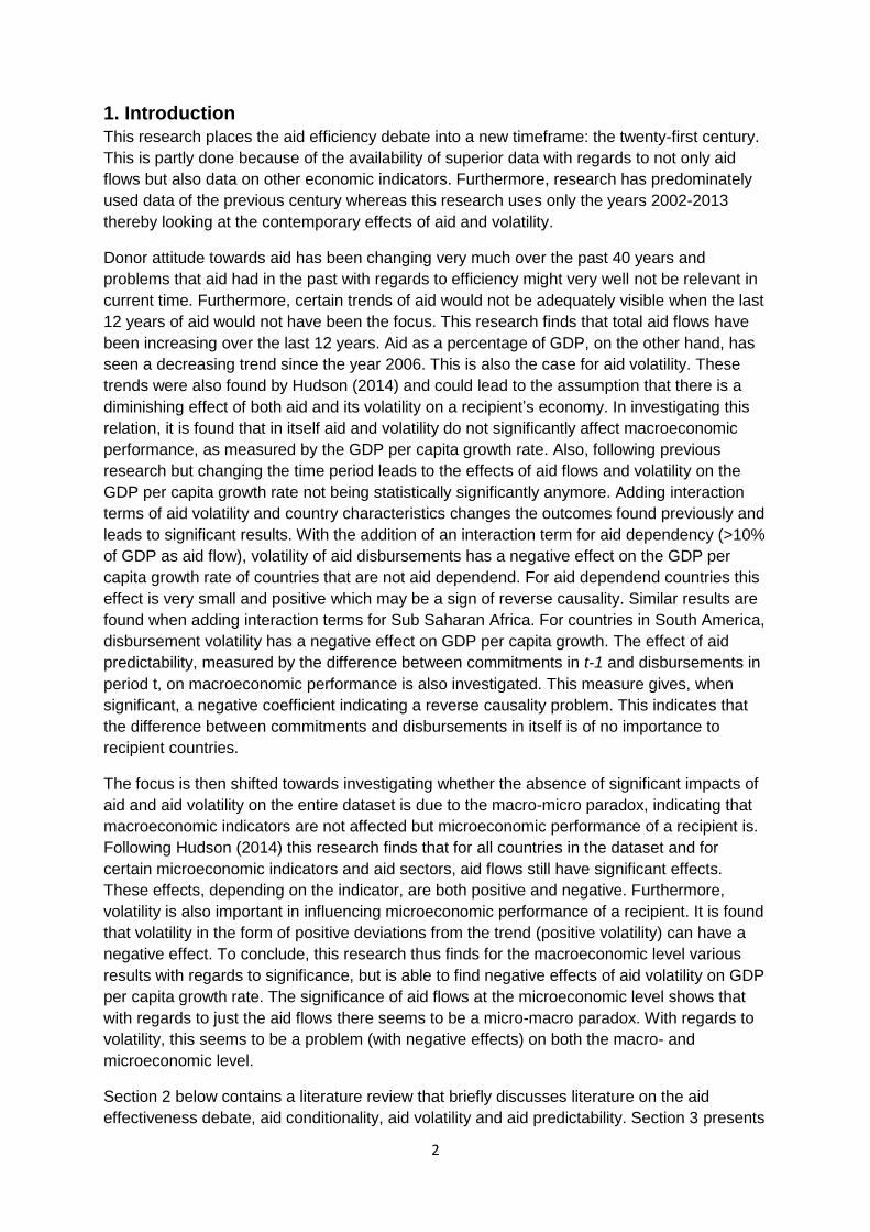
Looking at total aid flows it is clear that disbursements do not simply follow commitments

made in the previous period. Aid flows have, since 2002, shown a clear upward trend with

both types of aid flows. For disbursements there is a large peak in 2006 which is caused by a

14

large increase in aid targeted at debt relief and focused on certain African countries. This

peak is not present for aid commitments, indicating that the large increase in disbursements

was not previously anticipated. Total aid flows over the period 2002-2013 are as depicted in

figure 1 below, where the graph for commitments is lagged so that in 2002, the value for

commitments made in 2001 is shown. Total aid commitments are lower than the following

disbursements for only three of the twelve periods, being higher in the rest. This indicates

that when it comes to total aid flows commitments are not a good indicator for what is going

to be disbursed, meaning that aid is highly unpredictable.

Figure 1: Total aid flows in the form of commitments and disbursements, where commitments lagged.

Within this dataset, both commitments and disbursements are expressed as a percentage of

the recipients GDP at the time of the actual commitment/disbursement. Table 2 shows a

short summary of the country-level aid flows and shows that even though the minimum and

mean value for commitments are higher, the maximum value of aid disbursements is the

highest with almost 185% of total GDP. This already shows that, with regards to aid

predictability, aid disbursements can be higher than the promised aid that was supposed to

be disbursed. This confirms the finding by Celasun and Walliser (2007) that is not only the

case that donor countries do not live up to the commitments but actually also disburse more

than promised. Lagged commitments and disbursements as shares of GDP have a

correlation coefficient of 0.78, indicating that they are indeed closely related but still have a

rather large difference between them.

Table 2: Summary of aid flows

Variable

Number of

observations Mean Min Max

Disbursements (as a % of

GDP) 1652 8.462 .001 184.911

Commitments (as a % of

GDP) 1652 8.913 .001 173.557

Table 1 in the appendix shows the results from seperately regressing commitments and

disbursements on a trend and a squared trend to make a non-linear trend of aid-flows. The

regression results, graphically shown in figure 2 below, show that, when using fixed effects

0

20000

40000

60000

80000

100000

120000

140000

160000

2002 2003 2004 2005 2006 2007 2008 2009 2010 2011 2012 2013

Total Disbursments Total Commitments

15

panel regression to allow for systematic country differences, there is an increasing trend with

regard to both commitments and disbursements up until around the year 2005 for

commitments and 2006 for disbursements. After that, aid flows (as a percentage of GDP)

sharply decrease and follow a negative trend. This decreasing trend is as indicated by the

negative coefficient for the squared time trend. Please note that the coefficients of aid

commitments are not statistically significant at the 5% level, this then means that with

regards to commitments it is not certain that there is a trend within countries.

Figure 2: Trends in total aid commitments and disbursements.

Note: Trends calculated through predicted values of trend model of table 1 in the appendix

4.3 Sector aid flows

Aid sector is a term coined by the OECD and indicates the sector of an economy that the aid

flow is supposed to help. For example, social infrastructure aid is aimed towards helping

infrastructure within the recipient country, which can be in the form of internet connections or

other forms of communication. What follows from this is that the aid flows that are as

specifically directed can possible be shown to have an effect on the microeconomic

performance of a country. Thus analysis can be used to investigate the relationship between

sector specific aid flows and more specified economic indicators. Table 2 in the appendix

shows an overview of the 10 major sectors that are of interest for this research and explain

their contents by stating some subsectors and a short description.

The dataset is compiled by looking at the availability of total aid flows. The sector specific aid

flows are not as well documented, or are not always present. This leaves this part of data

with quite a few holes, which is shown by the number of observations. Furthermore, sector

aid flows as a percentage of GDP are often times very small, this is because there are ten

sectors over which aid is divided, and not every sector gets an equal amount of aid flows at

any given time. The summary of sector specific aid flows is given by table 3. As shown by the

67

89

10

2000 2005 2010 2015year

Trend in commitments Trend in total disbursements

16

mean of both disbursements and commitments, most aid goes towards social infrastructure

and service aid. Not coincidentally, this is also the sector that has the most available data

and therefore a sector that is always of interest to donors. For debt aid and aid aimed

towards helping refugees in donor countries there is the least data available. This is due to

then this type of aid not often being used and thus there are relatively few observations. Debt

aid, however, does have the highest maxima as a percentage of GDP for both

disbursements and commitments. When it comes to aid aimed at economic infrastructure the

maximum value for commitments is more than doubled by the maximum amount of

disbursements. This can mean that aid aimed at this sector is often highly conditional and is

not often paid out, which is also shown by a higher mean.

Table 3: Summary of sector aid flows

Flow type Disbursements Commitments

Sector Number of

observations Mean Min Max

Number of

observations Mean Min Max

Social

infrastructure 1652 3.654 0.001 78.240

1652 3.198 0.00061 64.700

Economic

infrastructure 1622 1.419 1.81E-06 71.660

1633 0.946 -0.02372 29.770

Production

sectors 1638 0.618 3.67E-06 9.842

1646 0.493 0.00003 23.181

Multi-sector 1643 0.901 0.0000278 58.376

1640 0.717 0.00003 44.276

Commodity

aid 1176 1.297 1.85E-09 42.856

1241 1.176 5.65E-08 44.790

Debt aid 830 1.137 2.77E-06 86.774

875 2.549 -0.0081 140.418

Humanitarian 1510 0.657 2.25E-06 33.980

1531 0.579 -0.0114 31.859

Admin costs

of donors 1425 0.028 1.81E-07 0.745

1475 0.034 1.81E-07 5.535

Refugees in

donor

countries

834 0.036 1.51E-07 2.252

853 0.036 8.89E-08 2.256

Unspecified 1559 0.066 5.11E-08 2.883 1614 0.164 -0.1984 5.281

As was the case with total aid flows, the majority of trends found in the sector aid flows are at

first positive but decreasing thereafter, indicating that as a percentage of GDP aid flows are

steadily decreasing. This decreasing trend can come from either total aid flows (not as a

percentage of GDP) also showing a decreasing trend or the GDP of recipient countries rising

faster than the aid flows, indicating a higher trend in GDP. Commitments of sector aid show 4

out of 10 significant trends at the 5% confidence level, of which 4 start positive become

decreasing trends. For the commitments of unspecified aid, however, it is reverse. There is a

negative trend that is becoming positive. Disbursements share the same trend for social

infrastructure and services and multi-sector aid with commitments. Disbursements however

also has a significant trend in the sector called administration costs of donor, where

commitments show no significant trend. There is no significant negative or positive trend in

either unspecified sector aid or debt aid for disbursements, even though these are present

17

within commitments. The difference in trends reinforces the conclusion that commitments are

not a good way to predict disbursements and expands that conclusion to sector specific aid.

The regression results corresponding to these trends are as shown by both table 2 and 3 in

the appendix, the former containing trends of commitments and the latter containing

disbursements. Figures 3 to 6 graphically show the trends in aid flows for those trends that

were statistically significant at the 5% confidence level.

Figure 3: trends for both social infrastructure commitments and disbursements

Note: Trend lines are calculated by predicted values of trend models found in table 3 and 4 in the appendix

Figure 4: trend for both commitments and disbursements for multi-sector aid

Note: Trend lines are calculated by predicted values of trend models found in table 3 and 4 in the appendix

2.5

33.5

4

2000 2005 2010 2015year

Social infrastructure commitments Social infrastructure disbursements

.4.6

.81

1.2

2000 2005 2010 2015year

Multi-sector aid commitments Multi-sector aid disbursements

18

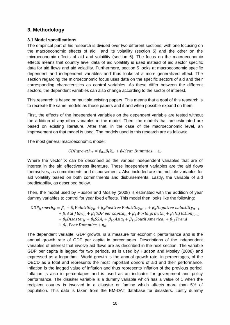
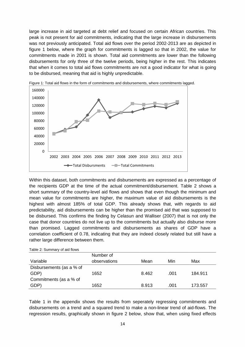
Figure 5: the trend of disbursements of administration costs of donors

Note: Trend lines are calculated by predicted values of trend models found in table 3 and 4 in the appendix

Figure 6: trends for the commitments of debt aid and of unspecified aid

Note: Trend lines are calculated by predicted values of trend models found in table 3 and 4 in the appendix

As shown by the images above the periods in which the trends change their sign differ from

sector to sector. Social infrastructure aid follows total aid flows with a decreasing trend

starting at around 2006. Multi-sector aid starts decreasing at around 2009 as does the

disbursements of administration cost aid. Debt aid too follows total aid flows with a decrease

in aid flows as a percentage of GDP starting around 2006. Unspecified aid commitments are

the only sector to start with a negative trend, which seems to become positive at around

2011.

.015

.02

.025

.03

.035

Adm

inis

tra

tion

co

sts

dis

burs

em

en

ts

2000 2005 2010 2015year

-10

12

34

2000 2005 2010 2015year

Debt aid commitments Unspecified aid commitments

19

4.4 Aid volatility

Measuring aid volatility follows from the previous sections in which the trends of aid flows are

calculated. Deviations from this trend, calculated per country, are considered aid volatility

and can either be positive or negative depending on the deviation from the trend. Squaring

these residuals gives the absolute positive value of aid volatility. Positive and negative

volatility, however, are also of interest; literature has found a significantly different effect

between the two. This way of measuring aid volatility, by calculating a trend over the years of

interest, assumes that the trend that starts at 2002 for this dataset is known by the recipient

country and has not been necessarily different in the period before. Because aid volatility is

measured using aid flows as a share of GDP, the residuals that represent volatility are as

percentage of GDP deviations from the aid flow trend. Using the squared residuals, as is

done by Hudson (2014) and in this research, makes the coefficient a little harder to interpret,

but the sign and significance of volatility are the main interest. Using the positive and

negative values for volatility makes it possible to interpret the results in the form of

percentage of GDP deviations.

The measures for positive and negative volatility are calculated with an upper bound of zero

for negative, and a lower bound of zero for positive aid volatility. This means that, for

example, when in period t in country j there is no observation for positive volatility (because

there is negative volatility), positive volatility gets an observation equal to zero. Imposing

these bounds makes it possible to include both variables in a model at the same time to

investigate their joint effect. Table 6 summarizes the volatility measures of total aid flows for

both commitments (upper three rows) and disbursements (lower three rows). Disbursements

show higher volatility than commitments in all three measures and indicate that there is a

predictability issue with aid volatility. It is therefore relevant to study both disbursements and

commitments, as they are both significantly different and can potentially influence recipient‟s

differently.

Table 4: summary of total aid flow volatility

Variable Number of

observations Mean Min Max

Squared commitment volatility 1642 26.493 4.37E-27 7507.299

Negative commitment volatility 1642 -1.041 -39.933 0

Positive commitment volatility 1642 1.041 0 86.645

Squared disbursement

volatility 1651 48.468 7.44E-24 12363.29

Negative disbursement

volatility 1651 -1.207 -52.101 0

Positive disbursement volatility 1651 1.207 0 111.190

Table 5 summarizes the three volatility measures for the different aid sectors. As is the case

with aid flows, total volatility is divided over the different sectors. The last three sectors

(Admin costs of donors, refugees in donor countries and unspecified aid) portray the lowest

volatility in aid flows, as can be seen from the minimum and maximum values for respectively

the negative and positive measures for volatility. Aid flows that are directed at debt have, as

seen in the previous section, the highest maximum and minimum values of all the different

20

aid sectors. This can also be seen in the measures for volatility; both the lowest negative

volatility and the highest positive volatility are seen in debt aid for commitments. The highest

positive volatility of disbursements is of economic infrastructure aid, the lowest is again debt

aid. The highly positive volatility of economic infrastructure specific aid disbursements is also

shown by the large difference in maximum commitments and disbursements of aid flows for

that sector. As argued before this shows that this type of aid is very unpredictable. The same

is the case for volatility.

Table 5: Summary of sector specific volatility measures

Flow type Disbursements Commitments

Sector Volatility

measure Obs Mean Min Max Obs Mean Min Max

Social

infrastructure

Squared 1652 4.590 1.21E-24 1834.256

1652 2.650 1.42E-24 1354.685

Positive 1652 0.441 0 42.828

1652 0.267 0 36.806

Negative 1652 -0.441 -15.189 0.000

1652 -0.267 -13.479 0.000

Economic

infrastructure

Squared 1622 6.333 1.92E-33 2290.632

1633 0.717 5.03E-26 300.613

Positive 1622 0.420 0 47.861

1633 0.151 0 17.338

Negative 1622 -0.420 -28.590 0.000

1633 -0.151 -10.259 0.000

Production

sectors

Squared 1638 0.369 6.97E-23 40.492

1646 0.220 1.96E-34 92.560

Positive 1638 0.155 0 6.363

1646 0.084 0 9.621

Negative 1638 -0.155 -3.010 0.000

1646 -0.084 -8.144 0.000

Multi-sector

Squared 1643 2.713 1.94E-25 1231.013

1640 1.474 1.25E-26 580.377

Positive 1643 0.209 0 35.086

1640 0.119 0 24.091

Negative 1643 -0.209 -16.128 0.000

1640 -0.119 -13.106 0.000

Commodity aid

Squared 1176 2.204 6.61E-39 1036.221

1241 1.833 7.35E-36 1148.054

Positive 1176 0.297 0 32.190

1241 0.225 0 33.883

Negative 1176 -0.297 -8.235 0.000

1241 -0.225 -8.296 0.000

Debt aid

Squared 830 12.964 2.22E-35 2073.595

875 64.169 1.96E-38 12329.880

Positive 830 0.518 0 45.537

875 1.505 0 111.040

Negative 830 -0.518 -39.325 0.000

875 -1.505 -50.174 0.000

Humanitarian

aid

Squared 1509 1.741 3.60E-38 485.599

1531 1.191 8.45E-33 415.974

Positive 1509 0.165 0 22.036

1531 0.133 0 20.395

Negative 1509 -0.165 -17.346 0.000

1531 -0.133 -10.038 0.000

Admin costs of

donors

Squared 1425 0.001 9.22E-36 0.087

1475 0.007 9.22E-36 5.592

Positive 1425 0.004 0 0.295

1475 0.006 0 2.365

Negative 1425 -0.004 -0.220 0.000

1475 -0.006 -1.773 0.000

Refugees in

donors

Squared 832 0.014 1.49E-38 3.445

850 0.012 1.84E-38 3.455

Positive 832 0.017 0 1.856

850 0.015 0 1.859

Negative 832 -0.017 -0.850 0.000

850 -0.015 -0.738 0.000

Unspecified

Squared 1559 0.010 2.70E-34 4.560

1614 0.042 6.49E-25 6.460

Positive 1559 0.016 0 2.136

1614 0.043 0 2.542

Negative 1559 -0.016 -0.705 0.000 1614 -0.043 -1.208 0.000

21

As mentioned before, total volatility is caused by the individual volatility of the different aid

sectors. As is done by Hudson (2014) the sum of the means of sector volatilities should

come close to the value of total volatility. If this is a perfect match, it would mean that total

volatility is caused only by volatility in the separate sectors. A difference between the two

indicates there is a covariance of the sectors and thus means that there is also interaction

within the sectors affecting total volatility. Table 6 shows the results of summing the mean

values of the different volatilities as they are depicted by table 4 and 5.

Table 6. Total aid flow volatility in a fixed effects model on sector specific aid flow volatilities

Disbursements Commitments

Squared Positive Negative

Squared Positive Negative

Social

infrastructure 4.590 0.441 -0.441

2.650 0.267 -0.267

Economic

infrastructure 6.333 0.420 -0.420

0.717 0.151 -0.151

Production sectors 0.369 0.155 -0.155

0.220 0.084 -0.084

Multi-sector 2.713 0.209 -0.209

1.474 0.119 -0.119

Commodity aid 2.204 0.297 -0.297

1.833 0.225 -0.225

Debt aid 12.964 0.518 -0.518

64.169 1.505 -1.505

Humanitarian aid 1.741 0.165 -0.165

1.191 0.133 -0.133

Admin costs of

donors 0.001 0.004 -0.004

0.007 0.006 -0.006

Refugees in

donors 0.014 0.017 -0.017

0.012 0.015 -0.015

Unspecified 0.010 0.016 -0.016

0.042 0.043 -0.043

Sum of sectors 30.938 2.244 -2.244 72.316 2.547 -2.547

Total volatility 48.468 -1.207 1.207 26.493 -1.041 1.041

For both disbursements and commitments it is the case that the sum of mean sector

volatilities is lower than the mean of total volatility. This thus, as argued above, indicates that

there is a covariance between the separate sectors that influences the value of total volatility.

4.5 Trends in aid volatility

Lastly, trends in volatility are investigated. Since research on the effects of aid volatility is

relatively new, Bulíř and Hamann (2008) found no decrease in volatility following their

research of 2003. Hudson (2014) also investigated this problem and found that, as is the

case with aid flows in this research, aid volatility had a significant non-linear trend that

increases up until around 2006 after which it sharply decreases. This research uses the

same database as Hudson (2014), albeit upgraded to around half more years of

observations, so the trends found by Hudson (2014) should still apply here. As done in the

previous sections, measures of aid volatilities are regressed on a time trend and its square

using a fixed effects panel model to control for country fixed characteristics. The coefficients

coming from these regressions are then used to graphically indicate the trend of volatility.

Following Hudson (2014), instead of using the squared measure for volatility the square root

of this value is used. This is done because the square measure is more influenced by outliers

and therefore prone to influence the trend. Regression results are as indicated in table4

through 6 in the appendix. The trends of volatilities that were significant at the 5% confidence

level are presented in figures 7 to 10.

22

Figure 7: Trends in volatility of both commitments and disbursements for unspecified sector aid

Note: Trend lines are calculated by predicted values of trend models found in table 5 and 6 in the appendix

Figure 8: Trends in Economic infrastructure commitment volatility and social infrastructure disbursement volatility

Note: Trend lines are calculated by predicted values of trend models found in table 5 and 6 in the appendix

0

.05

.1.1

5.2

2000 2005 2010 2015year

Unspecified aid commitments Unspecified aid disbursements

.2.4

.6.8

1

2000 2005 2010 2015year

Economic infrastructure commitments Social infrastructure disbursements

23

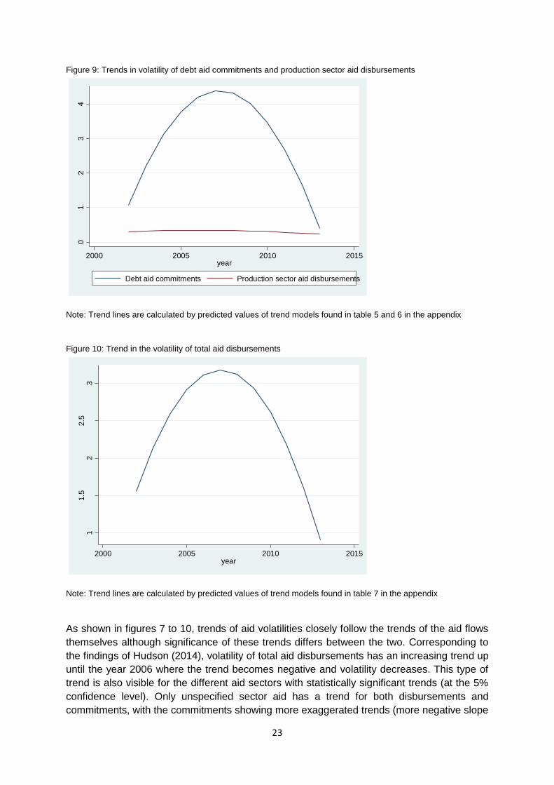
Figure 9: Trends in volatility of debt aid commitments and production sector aid disbursements

Note: Trend lines are calculated by predicted values of trend models found in table 5 and 6 in the appendix

Figure 10: Trend in the volatility of total aid disbursements

Note: Trend lines are calculated by predicted values of trend models found in table 7 in the appendix

As shown in figures 7 to 10, trends of aid volatilities closely follow the trends of the aid flows

themselves although significance of these trends differs between the two. Corresponding to

the findings of Hudson (2014), volatility of total aid disbursements has an increasing trend up

until the year 2006 where the trend becomes negative and volatility decreases. This type of

trend is also visible for the different aid sectors with statistically significant trends (at the 5%

confidence level). Only unspecified sector aid has a trend for both disbursements and

commitments, with the commitments showing more exaggerated trends (more negative slope

01

23

4

2000 2005 2010 2015year

Debt aid commitments Production sector aid disbursements

11.5

22.5

3

Vola

tilit

y o

f to

tal aid

dis

burs

em

en

ts

2000 2005 2010 2015year

24

at the start, more positive slope at the end). The trend reversal for this sector is, as was the

case for normal aid flows, a few years later than the change of trend for the other sectors. As

mentioned before, the year 2006 has a massive peak in total aid flows due to a sharp

increase in disbursements of debt aid.

5. Empirical macroeconomic analysis and results

This section analyzes the effects of aid flows, aid volatility and aid predictability on the

macroeconomic performance of the countries that are included in the dataset.

Macroeconomic performance is represented as GDP per capita growth because GDP per

capita is a widely used indicator for welfare and thus its growth rate indicates changes in

welfare. Annual GDP per capita growth is used for all analyses in this section as the

dependent variable. Research on this topic is not new and has been investigated in almost

every study regarding this topic. However, most of these other studies use different datasets

with data coming from different databases. This research uses the CRS database, which is

arguably the most reliable database to date with regards to aid flows. Furthermore, the

measure of volatility used for this research is not the Hodrick-Prescott filter and thus differs

from existing literature analyzing country-level mechanisms of aid volatility.

5.1 First look at aid, volatility and predictability

Starting with the most general estimations, the results of regressing GDP growth on aid

flows, aid volatility and aid predictability are shown in table 7. All regressions use fixed

effects to control for country-specific characteristics. Furthermore dummies are added for the

years, as indicated by the testparm application in Stata, to control for time-fixed effects. As

indicated by a modified Wald test, there is heteroskedasticity so robust and clustered

standard errors are also used. With no control variables present, total aid flows and aid

volatilities do not have a statistically significant effect on GDP growth. Interestingly aid

predictability does. Aid predictability is the difference between disbursements in period t

minus the commitments in period t-1. This then means that when aid is fully predictable its

value should be equal to zero. Any change in predictability thus makes it less predictable.

The significant negative effect of the predictability measure on the GDP per capita growth

rate indicates a possible reverse causality as this negative coefficient would mean that giving

less disbursements than commitments would actually benefit a country. This is not logical

and therefore leads to the assumption that the sign of this coefficient is most probably

caused by increases in disbursements compared to commitments that follow from a

decrease in GDP per capita growth rate. As stated, these results are all of country-fixed

effects. For completeness, results for both normal OLS (non-panel) and random effect panel

estimations are presented in tables 8 and 9 in the appendix.

So, with regards to their effects in the most general models, variables pertaining aid flows as

used by most research seem to be of no significance in affecting the annual GDP per capita

growth rates of the countries included in this research for the 2002-2013 period. This can

have several reasons, most importantly the small size of the model which captures a too

small variation in such a large macroeconomic indicator as GDP per capita growth. The next

section eliminates this problem by estimating a full model as given by Hudson and Mosley

(2008).

25

Table 7: General regressions of aid flows, aid volatility and aid predictability

Variables Annual GDP per capita growth rate

Disbursements 0.005

(0.01)

Commitments (lagged)

0.056

(0.04)

Disbursement volatility

-4.76e-05

(0.0003)

Commitment

volatility(lagged)

0.001

(0.001)

Predictability

-0.025**

(0.01)

Constant 1.837*** 1.964*** 1.908*** 2.406*** 2.436***

(0.39) (0.59) (0.40) (0.42) (0.41)

Observations 1,639 1,505 1,638 1,496 1,498

R-squared 0.055 0.061 0.058 0.057 0.057

Number of countries 143 143 143 142 143

Note: Robust and clustered standard errors in parentheses, *** p<0.01, ** p<0.05, * p<0.1

Dependent variable is GDP per capita growth rate, estimations are fixed effects

5.2 Following Hudson and Mosley

Following these basic results of different aid flows is replicating the results as found by

Hudson and Mosley (2008). Their paper follows up Bulíř and Hamann (2003, 2008) and

expands on it by using measures for positive and negative volatility and increasing the size of

the dataset. This research follows in that it uses the same variables and model. The

important difference is that the time period is different from their research, as well as this

research includes a larger number of countries. This automatically means that recreating

their model should not necessarily give similar results. It is, however, interesting to see

whether their results and conclusions are still applicable in this time period.

Tables 10 and 11 of the appendix show the results for the estimated models based on

Hudson and Mosley (2008). Table 10 indicates aid flows in the form of commitments and

table 11 contain the disbursements. Control variables are similar for both models and are as

described above. The second columns are the regular OLS results, added for completeness.

A Breusch-Pagan langragian multiplier test is done to see whether using random effects

panel estimations are superior to OLS, and this is confirmed. Hausmann tests are used to

see whether the fixed effects models of the fourth columns are a better fit than random

effects estimations. This results in a test statistic probability of 0.0005 for disbursements and

0.000 for commitments, indicating fixed effects is the best fit. Furthermore, this dataset

consists of time-series data and thus autocorrelation can be a problem within the data, this is

however largely countered by using robust and clustered standard errors. The fifth and sixth

columns show the results for the AR(1) estimations of both the fixed and random effects

estimations, this means that for both these estimated models the lagged dependent variable

is added into the model. This is, however, only done for completeness sake.

The fixed effects models estimated (column 4 in both table 10 and 11) show little similarity to

the results found by Hudson and Mosley (2008). This is due to the difference in data but can

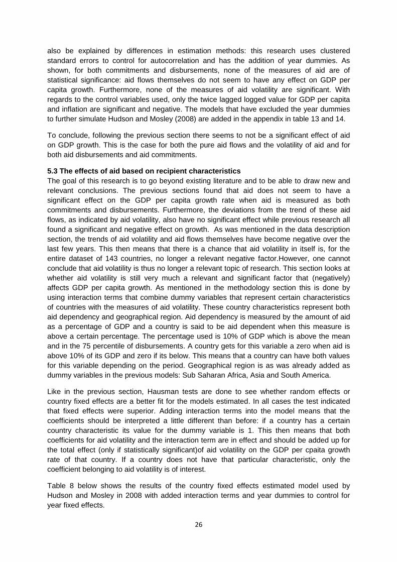
26

also be explained by differences in estimation methods: this research uses clustered

standard errors to control for autocorrelation and has the addition of year dummies. As

shown, for both commitments and disbursements, none of the measures of aid are of

statistical significance: aid flows themselves do not seem to have any effect on GDP per

capita growth. Furthermore, none of the measures of aid volatility are significant. With

regards to the control variables used, only the twice lagged logged value for GDP per capita

and inflation are significant and negative. The models that have excluded the year dummies

to further simulate Hudson and Mosley (2008) are added in the appendix in table 13 and 14.

To conclude, following the previous section there seems to not be a significant effect of aid

on GDP growth. This is the case for both the pure aid flows and the volatility of aid and for

both aid disbursements and aid commitments.

5.3 The effects of aid based on recipient characteristics

The goal of this research is to go beyond existing literature and to be able to draw new and

relevant conclusions. The previous sections found that aid does not seem to have a

significant effect on the GDP per capita growth rate when aid is measured as both

commitments and disbursements. Furthermore, the deviations from the trend of these aid

flows, as indicated by aid volatility, also have no significant effect while previous research all

found a significant and negative effect on growth. As was mentioned in the data description

section, the trends of aid volatility and aid flows themselves have become negative over the

last few years. This then means that there is a chance that aid volatility in itself is, for the

entire dataset of 143 countries, no longer a relevant negative factor.However, one cannot

conclude that aid volatility is thus no longer a relevant topic of research. This section looks at

whether aid volatility is still very much a relevant and significant factor that (negatively)

affects GDP per capita growth. As mentioned in the methodology section this is done by

using interaction terms that combine dummy variables that represent certain characteristics

of countries with the measures of aid volatility. These country characteristics represent both

aid dependency and geographical region. Aid dependency is measured by the amount of aid

as a percentage of GDP and a country is said to be aid dependent when this measure is

above a certain percentage. The percentage used is 10% of GDP which is above the mean

and in the 75 percentile of disbursements. A country gets for this variable a zero when aid is

above 10% of its GDP and zero if its below. This means that a country can have both values

for this variable depending on the period. Geographical region is as was already added as

dummy variables in the previous models: Sub Saharan Africa, Asia and South America.

Like in the previous section, Hausman tests are done to see whether random effects or

country fixed effects are a better fit for the models estimated. In all cases the test indicated

that fixed effects were superior. Adding interaction terms into the model means that the

coefficients should be interpreted a little different than before: if a country has a certain

country characteristic its value for the dummy variable is 1. This then means that both

coefficients for aid volatility and the interaction term are in effect and should be added up for

the total effect (only if statistically significant)of aid volatility on the GDP per cpaita growth

rate of that country. If a country does not have that particular characteristic, only the

coefficient belonging to aid volatility is of interest.

Table 8 below shows the results of the country fixed effects estimated model used by

Hudson and Mosley in 2008 with added interaction terms and year dummies to control for

year fixed effects.

27

Table 8: Regressions results of the models including interaction terms

Disbursements Commitments

VARIABLES

Aid >10%

GDP SSA Asia

South

America

Aid >10%

GDP SSA Asia

South

America

Trend 0.243 0.0905 0.0624 0.107

0.301 0.340 0.166 0.322

(1.48) (1.48) (1.48) (1.48)

(1.45) (1.43) (1.43) (1.44)

Disaster -0.406 -0.411 -0.396 -0.334

-0.384 -0.360 -0.394 -0.391

(0.28) (0.28) (0.28) (0.26)

(0.28) (0.28) (0.28) (0.28)

Aid flow -0.0241 -0.00569 -0.0134 -0.00935

0.0340 0.0212 0.0290 0.0309

(0.02) (0.02) (0.02) (0.02)

(0.03) (0.03) (0.02) (0.02)

Inflation (t-1) -0.0748** -0.0745** -0.0734** -0.0728**

-0.0841** -0.0814** -0.0797** -0.0842**

(0.03) (0.03) (0.03) (0.04)

(0.04) (0.04) (0.04) (0.04)

Volatility -0.0298*** -0.00734*** -1.35e-05 -7.10e-05

0.0121 0.00985** -0.000216 -0.000246

(0.01) (0.002) (0.0003) (0.0003)

(0.02) (0.004) (0.001) (0.001)

Volatility*Dummy 0.0299*** 0.00726*** -0.00905 -0.0420***

-0.0124 -0.0100*** 0.0355 0.00511

(0.01) (0.002) (0.01) (0.01)

(0.02) (0.004) (0.02) (0.01)

Positive volatility 0.0287 0.0244 0.0256 0.0262

-0.00433 0.00151 -0.00282 -0.00456

(0.02) (0.02) (0.02) (0.02)

(0.03) (0.03) (0.03) (0.03)

Negative volatility -0.0716* -0.0534 -0.0604 -0.0589

0.109 0.0996 0.113 0.109

(0.04) (0.04) (0.04) (0.04)

(0.09) (0.09) (0.09) (0.09)

World growth -0.0959 -0.792 -0.929 -0.772

0.304 0.466 -0.370 0.400

(7.21) (7.22) (7.21) (7.20)

(7.05) (6.97) (6.99) (7.05)

log GDPPC -5.088*** -5.001** -5.006** -5.104***

-4.834** -4.908** -4.812** -4.862**

(1.93) (1.93) (1.93) (1.92)

(1.99) (1.98) (1.98) (1.98)

Constant 39.99 41.97 42.57 42.54

36.51 36.42 38.93 36.37

(30.54) (30.68) (30.66) (30.57)

(30.24) (30.03) (30.20) (30.28)

Observations 1,228 1,228 1,228 1,228

1,222 1,222 1,222 1,222

R-squared 0.099 0.099 0.097 0.101

0.099 0.101 0.101 0.099

Countries 132 132 132 132

131 131 131 131

Hausman prob>Chi: 0.000 0.000 0.0007 0.0007

0.000 0.000 0.0014 0.000

Note: Clustered and robust standard errors in parentheses, *** p<0.01, ** p<0.05, * p<0.1

Dependent variable is GDP per capita growth rate, estimations are fixed effects as indicated

by Hausman statistics

For commitments, only when the interactionterm of Sub Saharan Africa is added, is there any

relevant variable significant: volatility is positive, the interaction term is negative. This thus

means that for the countries that are not in Sub Saharan Africa, aid volatility of commitments

has a positive and significant effect on GDP per capita growth. This positive effect is

counterintuitive and indicates a possible reverse causality present in this estimation.

Countries that are situated in Sub Saharan Africa, on the other hand, have a significant but

negative effect (albeit a very small one). The latter is also found when looking at aid

disbursements. On the other hand, for all other countries it is the other way around: aid

volatility has a negative effect on the GDP per capita growth rate. For aid disbursements,

when the interaction term pertains aid dependency it is found that for countries that have aid

disbursements below 10% of their GDP, aid volatility has a significant negative effect. When

countries are aid dependend, this effect becomes positive but very small (almost zero). The

interaction term of aid volatility and countries in South America is also significant for

disbursements: it has a negative effect on the GDP per capita growth rate. Adding this

interaction term gives for disbursements the highest value of the R-squared, even though aid

volatility in itself (so for all other countries) is not statistically significant. The Hausman

probability statistics are given in the last row and indicate that for every model fixed effects is

the best estimation method.

28

5.4 The effect of aid predictability

Results of this research indicate mostly that there is a difference in the effects that both

disbursements and commitments have on GDP per capita growth. What follows is the idea

that recipient countries react to commitments when they are made and to disbursements

when they are received. Aid predictability can therefore be of interest with regards to aid

efficiency. Section 5.1 showed that by looking at the effects of aid variables in a model

without control variables, aid predictability had a negative effect on GDP per capita growth.

As argued there, this is an indication of reverse causality. This section of the research adds

that variable to the models of Hudson and Mosley (2008) to see whether predictability has

any effects on the GDP per capita growth rate, and if so if this is still an indication of the

reverse causality found in section 5.1 or whether there seems to be a mechanism in place

where recipient countries react to aid commitments in a way that lower disbursements would

have an effect on the economy. The results of the addition of predictability are shown in table

9. These results are also included in the appendix in table 17, which also included random

effects estimations.

Opposed to when no control variables are added into the model, predictability does not have

a significant effect on GDP per capita growth when it is added to the model on itself. The

introduction of an interaction term that represents aid dependency makes predictability

significant and again negative. The interaction term is significant and positive, with a smaller

absolute value than the coefficient for predictability. This indicates that for countries that are

not aid dependend and for countries that are, aid predicitability has a negative effect on the

GDP per capita growth rate. For the latter countries this effect is smaller. Again, as was the

case in section 5.1, this is an indication of reverse causality as a negative value for this

variables means that a recipient country getting less aid disbursed than was commited would

increase its GDP per capita growth rate. It is therefore highly probable that the effect shown

is due to decreases in the GDP per capita growth rate followed by an increase in

disbursements relative to commitments.

29

Table 9: Modelof Hudson and Mosley (2008) with the addition of predictability and an interaction term.

VARIABLES No interaction Aid > 10% GDP

Trend 0.0790 -0.0229

(1.476) (1.504)

Diaster -0.397 -0.396

(0.275) (0.284)

Aid flows -0.000672 -0.000855

(0.0296) (0.0278)

Inflation (t-1) -0.0741** -0.0702**

(0.0350) (0.0350)

Volatility -1.04e-05 -0.000147

(0.0003) (0.0003)

Predictability -0.0163 -0.191**

(0.0324) (0.0951)

Predictability*Aid dependency

0.187**

(0.0944)

Positive volatility (t-1) 0.0170 0.0199

(0.0160) (0.0154)

Negative volatility (t-1) -0.0671 -0.0610

(0.0502) (0.0476)

World growth -0.825 -1.372

(7.200) (7.340)

log GDPPC -4.926** -4.887**

(1.957) (1.947)

Constant 41.50 43.10

(30.76) (31.22)

Observations 1,228 1,228

R-squared 0.098 0.101

Countries 132 132

Note: Clustered and robust standard errors in parentheses, *** p<0.01, ** p<0.05, * p<0.1

Dependent variable is GDP per capita growth rate, estimates are fixed effects.

5.5 Statistical problems with models

Dalgaard, Hansen and Tarp (2004) argue that when using annual data for aid flows, aid may

not have an endogeneity problem. Hudson and Mosley further investigate this and conclude

that indeed aid is not endogenous. They do however still estimate their model using

instruments for aid, which does not give any different results from their models not using

instruments. It logically follows that aid is probably endogenous and that instrumental values

should be added to the models. However, the difficult part is in finding good instruments that

can be argued to fully capture this endogeneity. This has not been done before in research

and is beyond the scope of this research. The above models therefore follow the

aforementioned researches and assume that aid is not endogenous. It should therefore be

noted that the results found in this section are indications of what effects aid flows, aid

volatility and aid predictability can possibly have on the macroeconomic performance of a

recipient country. With regards to causality there is a similar problem. However, the signs of

the coefficients belonging to aid flows indicate that causality is indeed as is argued in the

30

theory above in that, when a statistically significant relation is found, aid influences

macroeconomic performance and not the other way around.

5.6 Summary

Replicating Hudson and Mosley‟s (2008) model finds no significant results for either aid flows

and measures of aid volatility. This is most probably due to the data used rather than the

estimation methods. This difference in found significance of the variables for aid and volatility

can be caused by the decreasing trends for both these variables found in section 4. The

effect of aid in itself has always been subject of discussion and this research finds no effect

for aid flows at the macroeconomic level. The next step is therefore to investigate whether

there is a macro-micro paradox in that aid flows influence a recipient‟s economy through

microeconomic performance rather than macroeconomic performance such as GDP per

capita growth. When expanding on the models of Hudson and Mosley (2008) by using

country characteristics it is found that aid volatility can have significant effects on countries,

in most cases negative. The positive effect of total volatility found for aid dependent countries

is counterintuitive and is possibly a sign of reverse causality. Models containing aid

predictability show reverse causality and indicate that the difference between commitments

and disbursements do not affect the recipients economic performance (at least not at the

macroeconomic level).

6. Empirical microeconomic analysis and results

This section investigates the effects of the sector-level aid flows and aid volatility on

microeconomic indicators that correspond to that sector. In table 2 of the appendix a

summary of all the sectors and their corresponding subsectors is given. Microeconomic

performance indicators are derived from these subsectors. Social infrastructure, for example,

can possibly be seen in government expenditure on health but also on death rates. Death

rates are as used by Hudson (2014), government expenditure on healthcare (public health

expenditure) are as suggested by van de Sijpe (2010). It should be noted that when looking

at these microeconomic indicators it is not necessarily the case that only the aid aimed at

that sector influences that specific indicator. As Hudson (2014) argues, not only aid aimed

towards helping healthcare decreases the death rates, but better education can also promote

healthier lifestyles. Furthermore it can be the case that a general better level of welfare

increases the average living standards of the recipient.

6.1 General models

Like the previous section, this section starts with the most generalized models of sector aid.

Not all sectors are included in this analysis due to not every sector having a suitable

microeconomic indicator that corresponds to it.

For the first estimations the focus is on the largest sector, social infrastructure and services,

with dependent variables corresponding to indicators that represent the effectiveness of aid

for this sector. This model therefore follows Hudson (2014) in using death rates and

secondary school completion rates. Regression results of random effects estimations are

given in table 18 in the appendix, country-fixed effects are given in table 19.

For death rates (log), estimations using a random effects panel model, which is the best fit

according to the Hausman tests, shows a significant and negative coefficient for negative

volatility of aid disbursements. Commitments, on the other hand, have only a significant

31

positive volatility, which has positive sign. The latter coincides with results previously found in

research.

For school completion, country fixed effects estimations are the best fit. However, these

estimations do not give any significant results when the aid flows are disbursements. For

commitments all three measures are significant, with aid commitments having a negative

effect. Both variables for volatility are positive. The negative effect of aid commitments is a

sign of reverse causality, an increase in aid would logically not be followed by a decrease in

school completion.

The second sector of interest is economic infrastructure. Mobile phones are used instead of

fixed telephone subscriptions because mobile phones have become more important over the

years and therefore fixed telephone subscriptions are likely to have been decreasing, which

is not being caused by the effects of aid but rather by an increase in technology. The number

of mobile phone subscriptions is logged to represent growth within the indicator. The results

corresponding to random effects estimations are given in table 20 in the appendix, country

fixed effects in table 21. None of the estimations are significant. Last for this sector is the

number of internet connections per 100 people to indicate the performance in

communications of the recipient country. This variable is used as a logged value. Table 20

and 21 also include these estimations. None of the estimations contain significant results.

Up until this point the analysis of sector-level effects of aid and volatility followed Hudson in

using the same indicators representing the sectors. This research now expands on Hudson

by including more, different sectors. Table 22 and 23 in the appendix contain the regression

results of the aid and volatility measures of the production sector aid on value added by

manufacturing, of multi-sector aid on CO2 emissions and finally of humanitarian aid on the

death rate for both random (table 24) and fixed effects (table 23) models. The latter

regression is added because humanitarian aid is a large and important sector of aid;

however there is no good indicator to represent what is done in this sector. Humanitarian aid

is aimed towards helping people after disasters, during wars or during famine. Humanitarian

aid can therefore arguably be represented by a decrease in death rate.

The aid flow variables do not influence the value added by the manufacturing sector,

whereas negative volatility has a negative effect. For CO2 emissions and multi-sector aid

there are no significant results at all. This is most probably due to CO2 emission not being

the best indicator representing this sector. However, no better were available. Humanitarian

aid disbursements seem to significantly influence the death rates. However, the actual

disbursements seem to have the wrong sign. This is due to reversed causality where an

increase in the death rate is followed by an increase in humanitarian aid. Volatility measures

of disbursements both have significant negative coefficients indicating that an increase in

volatility decreases the death rate.

32

6.2 Following Hudson

Due to the causality issues mentioned above, the focus is again shifted to the sectors and

indicators used by Hudson (2014). Recreating these models and extending the time period to

2013 instead of 2007 gives the results as presented in tables 24 (random effects) and 25

(fixed effects) of the appendix. The relevant results with regards to best fitting models and

results are given in table 10. The bottom row of table 10 contains the Prob>chi statistic of the

Hausman test to show why either RE or FE are used.

Table 10: Best fitted models following Hudson (2014).

Social Infrastructure aid Economic infrastructure aid

VARIABLES Death rate (log)

School completion

(log)

Mobile Phone (log) Internet (log)

Disbursements -0.00241** 0.00424 0.0646** 0.0789**

(0.00112)

(0.00327)

(0.0305)

(0.0335)

Disbursement volatility

(+) 0.00447***

-0.0128**

-0.0700*

-0.109**

(0.00135)

(0.00597)

(0.0361)

(0.0428)

Disbursement volatility

(-) -0.00223*

0.00142

-0.0351

0.00834

(0.00129)

(0.0118)

(0.0247)

(0.0333)

Aid commitments (t-1)

-0.00716***

-0.000825

0.0634

0.0832

(0.00196)

(0.00226)

(0.0425)

(0.0603)

Commitment volatility

(t-1, +)

0.00902***

-0.0215

-0.145***

-0.143**

(0.00218)

(0.0198)

(0.0544)

(0.0654)

Commitment volatility

(t-1, -)

0.00378*

0.0186

0.0399

0.0483

(0.00212)

(0.0193)

(0.0813)

(0.0532)

Total Aid

Disbursements 0.000161

-

0.00213*

-0.00145

-0.00264

(0.000227)

(0.00117)

(0.00211)

(0.00192)

Total Aid commitments

(t-1)

0.000617*

0.000851

-

0.000162

-0.00289

(0.000331)

(0.000588)

(0.00213)

(0.00214)

Base value of

dependent variable 0.918*** 0.918*** 0.770*** 0.748***

0.842*** 0.816*** 0.734*** 0.696***

(0.0163) (0.0176) (0.0274) (0.0283)

(0.0370) (0.0417) (0.0402) (0.0463)

Constant 0.181*** 0.177*** 0.907*** 1.055***

1.916*** 2.782*** 0.0868 0.432***

(0.0348) (0.0373) (0.112) (0.123)

(0.488) (0.562) (0.0613) (0.0738)

Observations 1,608 1,477 699 627

1,504 1,389 1,528 1,413

Number of country 141 140 78 78

133 133 136 136

Estimation Method RE RE RE RE

RE RE RE RE

Hausman Prob>chi 0.13 0.93 0.11 0.062

x 0.99 0.081 0.92

Note: Robust standard errors in parentheses, *** p<0.01, ** p<0.05, * p<0.1

For FE estimations, standard errors are clustered and robust. Year

dummies are excluded from the table due to size.

As shown in the second to last row, all models use random effects, as supported by the

Hausman tests of which the probabilities are in the last row. For mobile phone subscriptions,

the Hausman test was inconclusive for the aid disbursements. Random effects is used

because of the better fit of random effects for aid commitments.

Both disbursements and commitments have a significant and negative effect on the death

rate, indicating an increase in aid flows leads to a decrease in the death rate (or change

therein, as indicated by the log). Positive volatility has, for both measures of aid flows, also a

significant effect. This effect is positive, indicating volatility leads to increases in the rate of

33

deaths, even if this volatility is in the form of positive deviations from the trend. Negative

volatility has the opposite sign for both disbursements and commitments. This variable,

however, is only significant at the 10% level. Hudson (2014) also uses random effects for

these estimations and finds similar results.

Different from Hudson (2014), school completion is not divided over females and males. This

is done due to data availability. Aid commitments do not give any significant results.

Disbursements on the other hand give for positive volatility a significant and negative sign.

This means that a positive deviation from the trend of aid disbursements leads to a decrease

in school completion. Hudson (2014) found a significant and positive effect of aid

disbursements on school completions, which this research is unable to replicate. This is also

the case when, like Hudson (2014), a worse fitting fixed effects estimation is used.

Economic infrastructure aid disbursements lead to an increase in both mobile phone and

internet subscriptions. Positive volatility decreases both, but only the effect on internet

subscriptions is significant at the 5% level (mobile phone subscriptions at the 10% level). For

aid commitments, positive volatility has a negative and significant effect: when aid

commitments positively deviate from their trend, there is a decreases in the growth of mobile

phone and internet subscriptions.

Hudson uses for both these estimations random effects. Also, instead of aid aimed at

economic infrastructure and services as a whole, he uses subsectors. His conclusion at the

end of his research states that there is a possible spillover bewtween sectors and

subsectors. Effects found in the more specified subsectors can therefore arguably be found

when using data of the larger sectors. Results of this research are almost similar to the

results found by Hudson: Hudson finds significant positive effects of disbursements on both

internet subscriptions and mobile phone subscriptions. Positive volatility of disbursements

has for both researches a significant effect on internet subscriptions. There is a difference in

the other measures: Hudson finds a significant and positive effect of negative aid volatility on

internet use, opposed to no significance at all. For mobile phone subscriptions positive

volatility has a negative effect in Hudson‟s research, this research again finds no effect that is

significant at at least the 5% level (it is however significant at the 10% level).

6.3 Macro-micro paradox

To summarize, section 6.2 recreates the results found by Hudson (2014) to see whether

there is a significant effect of volatility on microeconomic indicators. As found by both

Hudson (2014) and this research, volatility has had a decreasing trend since the year 2006,

which continued for the entire time period used in this dataset. This is the case for total

volatility and for volatility of the different sectors. This research looks at whether these

negative trends have made volatility an insignificant inconsistency of aid flows. This is not the

case and aid volatility in both negative and positive form significantly affect microeconomic

indicators. Furthermore, aid flows affect these indicators. Section 5 found that aid flows, both

disbursements and commitments, do not have any significant effect on macroeconomic

performance. The combination of these results mean that there is likely to be a macro-micro

paradox: aid flows do not affect macroeconomic performance but recipient countries do

benefit from them in the form of microeconomic performance. Aid volatility has an effect on

both the macroeconomic and microeconomic level.

34

7. Conclusion and discussion

The goal of this research was to investigate the effects of aid flows, aid flow volatily, aid flow

predictability on macro- and microeconomic performance and to see whether it was still the

case that volatility has a negative effect on both economic performances. In short: to see

whether aid flows are effective. This research sets itself apart from other existing literature by

using both disbursements and commitments to investigate the effects of aid. Furthermore,

the CRS database is used which has only recently become available and has not been used

often. Research on both the macroeconomic and microeconomic level also gives the

opportunity to investigate the macro-micro paradox.

Despite recent literature stating aid is not effective and not efficient, total aid flows have had

a positive trend over the last 14 years, commitments closely following aid disbursements.

When aid flows are expressed as a percentage of the recipient‟s GDP this positive trend was

present up until around 2006. After 2006 this trend turns negative and aid flows as a

percentage of GDP seem to decrease. Coupled with the increasing trend of total aid flows

this leads to believe that, on average for this dataset, recipient countries have a faster

growing GDP than that there is an increase in aid flows. Aid recipient countries are by

definition not the most developed countries and part of this increase in GDP might be

contributable to aid.

Hudson(2014) investigated the trend of aid volatility and found that, although positive before,

in 2006 the trend of aid volatility has become negative. This research duplicates those results

and expands the number of years investigated from 2002-2007 to 2002-2013, thereby

confirming that the negative trend has continued. This negative trend could indicate a

diminishing effect of volatility, as volatility becomes smaller.

What follows is a country-level analysis of the effect of aid and volatility that is modeled after

previous research, most significantly Hudson and Mosley (2008), by recreating the models

used in that research and by changing the time period to 2002-2013 (due to the new

database used for data pertaining aid flows). These models, contrary to Hudson and Mosley

(2008), show no significant effect of aid or aid volatility on the GDP per capita growth rate of

a recipient country. These results were also already found by looking at the most general

effects of these measures on GDP per capita growth. The difference in outcome between the

two researches is most likely due to the difference in the time period.

Introducing interaction terms between volatility and terms that involve certain recipient

characteristics (aid dependency and whether countries are located in Sub Sahara Africa,

Asia or South America) changes the estimated coefficients of volatility with regards to the

significance. When an interaction term for aid dependency is added it is found that for

countries that receive less than 10% of their GDP in aid disbursements, volatility has a

negative effect on the GDP per capita growth rate. When countries receive more than 10% of

their GDP in disbursements, this effect is positive, but very small. A positive effect of total

volatility is not previously found in literature and counterintuitive, indicating a possible reverse

causality for this coefficient. These results show that aid volatility, despite its recent negative

trend, is still negatively influencing GDP per capita growth. This effect is found for countries

that are not aid dependent (aid disbursements of less than 10% of GDP) and countries that

are situated in South America. This effect is also found for the model that uses Sub Saharan

Africa as characteristic, countries that are situated in Sub Saharan Africa have a smaller

negative effect than countries that are outside of Sub Saharan Africa. Both are significant.

35

These results are only for disbursements. This indicates that aid volatility still has an effect

on the macroeconomic performance of an aid receiving country. This effect is negative, as

found by previous research.

Aid flows are still not significant and do not seem to influence macroeconomic performance

of a recipient in the form of GDP per capita growth. This is the case for all models estimated.

Lastly, on the macroeconomic level, predictability looks at how well disbursements follow

commitments. An increase in the variable for predictability would thus indicate a decrease in

how predictable aid is, regardless of whether it is positive or negative. Predictability has a

significant negative effect on GDP per capita growth when an interaction term regarding aid

dependency is added to the model. This negative effect is an indication of reverse causality.

This finding leads to the conclusion that the difference between commitments made and

disbursements received do not influence the recipients economy and indicates that recipient

countries do not seem to react to aid commitments in a way that lower aid disbursements

would negatively influence the economy.

On the microceconomic level, the estimated models show almost identical results to Hudson

(2014). Aid volatility affects different microeconomic indicators, such as the death rate,

school completion and subscriptions for mobile phones and internet, and thereby the

microeconomic performance of a recipient country. Furthermore, aid flows significantly affect

the death rate and mobile phone and internet subscriptions, indicating that aid is efficient

when it comes to these indicators. This supports the argument that aid flows are beneficial

for recipient countries even though this is not always visible on the macroeconomic level.

This confirms the argument for the existence of the macro-micro paradox.

To summarize, aid disbursements and aid commitments have a significant effect on

microeconomic performance. Volatility of aid flows can affect both the macroeconomic

performance and the microeconomic performance of a recipient country. To maximize their

efficiency, aid donors should aim to increase a recipient‟s microeconomic performance.This

will ultimately lead to better macroeconomic performance. This means that donor countries

should keep enforcing the conditionality of aid with regards to microeconomic goals and

make sure that aid flows are used to reinforce these conditions. Recipient countries, on the

other hand, should aim towards following these conditions as good and fast as possible to be

able to make aid as effective as possible. In doing this, deviations from the trend of aidflows

are kept as small as possible thereby decreasing aid volatility and thus the negative effects

volatility can have on both the macroeconomic and microeconomic level.

Following the results of this research, future research should investigate the implications of

the negative trend in aid volatility. The number of aidsectors investigated is also rather limited

in this research and should be expanded on in the future, when more data becomes

available in the CRS database. More data also means that microeconomic analysis can be

further specified with regards to subsectors and geographical regions. Furthermore, this

research finds for several models a reverse causality. This leads to the question whether

other results are also subject to this reverse causality. This is a problem that is present in this

kind of research, this subject of research in particular. Instrumental variable estimations can

be used to control for this reverse causality and endogeneity. However, scholars have yet to

find good instruments. Future research should therefore also aim towards finding these

instruments.

36

8. Reference list

Arellano, C., Bulíř, A., Lane, T. & Lipschitz, L., 2009, "The dynamic implications of foreign aid

and its variability" Journal of Development Economics 88: 87-102

Boone, P., 1996, "Politics and the Effectiveness of Foreign Aid." European Economic Review

40(2): 289-329

Bulíř, A. & Hamann, A.J., 2003, "Aid volatility: And Empirical Assessment" IMF Staff Papers

50(1): 64-89

Bulíř, A. & Hamann, A.J., 2008, "Volatility and development aid: From the frying pan into the

fire?" World Development 36(10): 2048-2066

Celasun, O. & Walliser, J., 2008 "Predictability of aid: Do fickle donors undermine economic

development?" IMF Finance and Development 45(3)

Chatterjee, S., Soukalis, G. & Turnovsky, S.J., 2003, "Unilateral capital transfers, public

investment and economic growth" European Economic Review 47(6): 1077-1103

Clemens, M.A., Radelet, S. & Bhavnani, R.R., 2004, "Counting Chickens when they Hatch:

The Short-term Effect of Aid on Growth" Center for Global Development Working Paper No.

44

Collier, P., Dollar, D., 2002, "Aid allocation and poverty reduction" European Economic

Review 46: 1475-1500

Dalgaard, C.J., Hansen, H & Tarp, F., 2004, “On the Empirics of Foreign Aid and Growth”

The Economic Journal 114(496):F191-F216

Collier, P., Guillaumont, P. Guillamon, S. & Gunning, J.W., 1997, "Redesigning conditionality"

World Development 25(9): 1399-1407

Easterly, W., 2005, "What did structural adjustment adjust? The association of policies and

growth with repeated IMF and World Bank adjustment loans" Journal of Development

Economics 76: 1-22

Fielding, D., 2007, "Aid and Dutch disease in the South Pacific" Research paper, UNU-

WIDER

Gale, D., 1974, "Exchange Equilibrium and Coalitions: an Example" Journal of Methematical

Economics 1: 63-66

Griffin, K., 1970, "Foreign Capital, Domestic Savings and Economics Development." Bulletin

of the Oxford University Institute of Economics and Statistics 32(2): 99-112

Hansen, H. & Tarp, F., 2000, "Aid effectiveness disputed" Journal of International

Development 12(3): 375-398

Hudson, J. & Mosley, P., 2008, "Aid Volatility, Policy and Development" World Development

36(10): 2082-2102

Hudson, J., 2014, "Consequences of Aid Volatility for Macroeconomic Management and Aid

Effectiveness" World Development

37

Keynes, J.M., 1929, "The German transfer problem." Economic Journal XXXIX: 1-7

Levy, V., 1988, "Aid and growth in Sub-Saharan Africa: The recent experience." European

Economic Review 32(9): 1777-1795

Mosley, P., 1980, "Aid savings and growth revisited" Oxford Bulletin of Economics and

Statistics 42(2): 79-95

Mosley, P., Huson, J. & Horrell, S., 1987, "Aid, the Public Sector and the Market in Less

Developed Countries" Economic Journal 97: 616-641

Neanidis, K.C. & Varvarigos, D., 2009, "The allocation of volatile aid and economic growth:

Theory and evidence" European Journal of Political Economy 25: 447-462

Panapek, G.F., 1973, "Aid, Foreign Private Investments, Savings and Growth in Less

Developed Countris." Journal of Political Economy 81(1): 120-130

Sijpe van de, N., 2013, "Is Foreign Aid Fungible? Evidence from the Education and Health

Sectors" World Bank Economic Review 27(2): 320-356

Singh, R.D. ,1985, “State intervention, foreign economic aid, savings and growth in LDCs:

Some recent evidence” Kyklos 38: 216-232

Temple, J.R.W., 2010, "Aid and conditionality" Handbook of Development Economics 5:

4415-4523

Weisskopf, T., 1972, "Impact of Foreign Capital Inflows on Domestic savings in Under

Developed Countries." Journal of International Economics 2:25-38

38

Appendix

Table 1: Trend regressions of aid disbursements and commitments.

Disbursements (as a % of GDP) Commitments (as a % of GDP)

Trend 320.6*** 128.1*

(83.44) (71.87)

Trend^2 -0.0799*** -0.0319*

(0.0208) (0.0179)

Constant -321,702*** -128,429*

(-83,748) (-72,14)

Observations 1,652 1,652

R-squared 0.012 0.005

Number of country 143 143

Standard errors in parentheses

*** p<0.01, ** p<0.05, * p<0.1

Table 2: Aid sectors and their subsectors

Sector Subsectors

Social infrastructure and services Education, health, population policy, water

supply and sanitation, government and civil

society

Economic infrastructure and services Transport, communications, energy, banking

and business

Production sector Agriculture, foresting fishing, industry and

trade policies

Multi-sector Environment protection and others

Commodity / program assistance General budget support

Debt aid Debt relief and forgiveness

Humanitarian Emergency response and reconstruction

Administration costs of donors No subsectors

Refugees in donor countries No subsectors

Unspecified No subsectors

39

Table 3: regression results of sector specific aid commitments as a percentage of GDP on a time trend and its square

Commitments

VARIABLES

Social

infrastructure

Economic

infrastructure

Production

sectors Multi sector Commodity Debt Humanitarian

Admin costs

of donors

Refugees in

donors Unspecified

Trend 107.1*** -4.720 -10.67 57.48*** -29.62 455.7*** 25.28* 1.488 -1.769 -25.25***

(22.38) (11.52) (6.523) (16.29) (26.68) (121.4) (14.23) (1.123) (1.814) (2.898)

Trend^2 -0.0267*** 0.00119 0.00265 -0.0143*** 0.00737 -0.114*** -0.00630* -0.000370 0.000439 0.00628***

(0.00558) (0.00287) (0.00162) (0.00406) (0.00665) (0.0302) (0.00354) (0.000280) (0.000452) (0.000722)

Constant -107,546*** 4,701 10,718 -57,718*** 29,767 -457,231*** -25,356* -1,495 1,784 25,386***

(22,468) (11,562) (6,547) (16,347) (26,782) (121,890) (14,287) (1,127) (1,820) (2,908)

Observations 1,652 1,633 1,646 1,640 1,241 875 1,531 1,475 853 1,614

R-squared 0.015 0.012 0.004 0.011 0.003 0.022 0.004 0.003 0.048 0.207

Number of countries 143 143 143 143 129 98 141 139 115 143

Standard errors in parentheses

*** p<0.01, ** p<0.05, * p<0.1

Table 4: Regression results of sector specific aid disbursements as a percentage of GDP on a time trend and its square

Disbursements

VARIABLES

Social

infrastructure

Economic

infrastructure

Production

sectors Multi sector Commodity Debt Humanitarian

Admin costs of

donors

Refugees in

donors Unspecified

Trend 126.5*** -21.25 -0.677 44.71** -26.03 68.99 11.21 1.269*** -0.0805 -0.244

(28.07) (28.69) (7.014) (20.16) (27.32) (61.32) (17.92) (0.388) (1.906) (1.282)

Trend^2 -0.0315*** 0.00531 0.000168 -0.0111** 0.00647 -0.0172 -0.00280 -0.000316*** 1.82e-05 5.96e-05

(0.00699) (0.00715) (0.00175) (0.00502) (0.00680) (0.0153) (0.00446) (9.66e-05) (0.000475) (0.000319)

Constant -126,947*** 21,261 682.4 -44,911** 26,177 -69,061 -11,206 -1,275*** 88.58 248.8

(28,170) (28,797) (7,040) (20,238) (27,420) (61,550) (17,985) (389.3) (1,914) (1,287)

Observations 1,652 1,622 1,638 1,643 1,176 830 1,510 1,425 834 1,559

R-squared 0.015 0.006 0.000 0.006 0.006 0.020 0.007 0.018 0.037 0.012

Number of countries 143 143 142 143 123 93 141 137 114 143

Standard errors in parentheses

*** p<0.01, ** p<0.05, * p<0.1

40

Table 5: trend estimations of volatility sector specific aid commitments by regressing volatility on a trend and its square

Commitments

VARIABLES Social

infrastructure

Economic

infrastructure

Production

sectors

Multi

sector

Commodit

y Debt

Humanitaria

n

Admin costs of

donors

Refugees in

donors Unspecified

Trend 16.36 17.54*** 0.0926 5.645 20.79* 484.9*** 4.191 0.824* 2.016* -7.565***

(10.81) (5.572) (3.053) (7.490) (11.33) (78.58) (7.776) (0.466) (1.110) (1.312)

Trend^2 -0.00408 -0.00437*** -2.47e-05 -0.00140 -0.00518* -0.121*** -0.00104 -0.000205* -0.000503* 0.00188***

(0.00269) (0.00139) (0.000760) (0.00187) (0.00282) (0.0196) (0.00194) (0.000116) (0.000276) (0.000327)

Constant -16,416 -17,611*** -86.02 -5,682 -20,871* -486,671*** -4,202 -827.1* -2,020* 7,602***

(10,852) (5,593) (3,065) (7,518) (11,377) (78,874) (7,806) (467.5) (1,114) (1,317)

Observation

s 1,652 1,633 1,646 1,640 1,241 875 1,531 1,475 850 1,614

R-squared 0.002 0.007 0.005 0.006 0.003 0.048 0.001 0.003 0.030 0.076

Number of

countries 143 143 143 143 129 98 141 139 114 143

Standard errors in parentheses *** p<0.01, ** p<0.05, * p<0.1

Table 6: trend estimations of volatility sector specific aid disbursements by regressing volatility on a trend and its square

Disbursements

VARIABLES Social

infrastructure

Economic

infrastructure

Production

sectors

Multi

sector Commodity Debt Humanitarian

Admin costs of

donors

Refugees in

donors Unspecified

Trend 35.45** 13.66 8.860** 5.837 21.13* 62.63* 6.713 0.0585 0.431 -1.478**

(14.04) (16.28) (3.769) (10.74) (12.51) (33.23) (9.305) (0.154) (1.186) (0.690)

Trend^2 -0.00884** -0.00340 -0.00221** -0.00145 -0.00527* -0.0156* -0.00167 -1.47e-05 -0.000109 0.000368**

(0.00350) (0.00405) (0.000939) (0.00267) (0.00312) (0.00828) (0.00232) (3.83e-05) (0.000295) (0.000172)

Constant -35,552** -13,739 -8,887** -5,877 -21,196* -62,744* -6,726 -58.15 -427.6 1,485**

(14,095) (16,336) (3,783) (10,776) (12,559) (33,353) (9,341) (154.5) (1,190) (692.2)

Observations 1,652 1,622 1,638 1,643 1,176 830 1,509 1,425 832 1,559

R-squared 0.008 0.003 0.007 0.004 0.005 0.029 0.002 0.017 0.040 0.008

Number of

countries 143 143 142 143 123 93 141 137 113 143

Standard errors in parentheses *** p<0.01, ** p<0.05, * p<0.1

41

Table 7: Non-linear trend estimations of the volatility of total aid disbursements and aid commitments Disbursements (as a % of GDP) Commitments (as a % of GDP)

Trend 257.1*** 44.75

(48.96) (32.41)

Trend^2 -0.0640*** -0.0112

(0.0122) (0.00807)

Constant -257,974*** -44,861

(49,141) (32,528)

Observations 1,652 1,642

R-squared 0.019 0.004

Number of country 143 142

Standard errors in parentheses

*** p<0.01, ** p<0.05, * p<0.1

42

Table 8: Model of section 5.1 using random effects

Variables Annual GDP per capita growth rate

Disbursements -0.0139

(0.0108)

Commitments (lagged)

0.00230

(0.0192)

Disbursement Volatility

-0.000107

(0.000313)

Commitments Volatility (lagged)

0.000412

(0.000859)

Predictability

-0.0291**

(0.0121)

Constant 1.930*** 2.401*** 1.852*** 2.408*** 2.433***

(0.444) (0.558) (0.458) (0.470) (0.458)

Observations 1,639 1,505 1,638 1,496 1,498

Number of countries 143 143 143 142 143

Note: Robust standard errors in parentheses, *** p<0.01, ** p<0.05, * p<0.1

Dependent variable is GDP per capita growth rate. Year dummies excluded from table

due to size

Table 9:Model of section 5.1 using OLS

Variables Annual GDP per capita growth rate

Disbursements -0.0223**

(0.00926)

Commitments (lagged)

-0.0124

(0.0104)

Disbursement Volatility

-0.000159

(0.000225)

Commitments Volatility (lagged)

7.98e-05

(0.000537)

Predictability

-0.0317**

(0.0135)

Constant 1.984*** 2.539*** 1.819*** 2.435*** 2.446***

(0.463) (0.465) (0.460) (0.459) (0.456)

Observations 1,639 1,505 1,638 1,496 1,498

R-squared 0.050 0.047 0.050 0.047 0.049

Note: Robust standard errors in parentheses, *** p<0.01, ** p<0.05, * p<0.1

Dependent variable is GDP per capita growth rate. Year dummies excluded from table

due to size

43

Table 10: Model by Hudson and Mosley (2008) of section 5.2, commitments.

VARIABLES OLS RE FE RE AR(1) FE AR(1)

Trend -1.355 -1.057 0.323 -0.114* 0.000311

(1.60) (1.54) (1.44) (0.07) (0.16)

Disaster -0.0842 -0.147 -0.393 -0.167 -0.537

(0.26) (0.30) (0.28) (0.38) (0.47)

Aid/GDP percentage (t-1) 0.0248 0.0236 0.0310 0.0233 0.0326

(0.02) (0.02) (0.02) (0.02) (0.04)

Inflation (t-1) -0.00950 -0.0228 -0.0842** -0.00850 -0.0589

(0.03) (0.03) (0.04) (0.03) (0.04)

Volatility (t-1) 0.000391 0.000330 -0.000247 0.000233 -0.000204

(0.00) (0.00) (0.00) (0.00) (0.00)

Positive Volatility (t-2) 0.000602 0.00191 -0.00464 0.000396 -0.0149

(0.02) (0.03) (0.03) (0.04) (0.06)

Negative Volatility (t-2) 0.138* 0.132 0.109 0.129* 0.144

(0.07) (0.10) (0.09) (0.07) (0.10)

World Growth -5.693 -4.214 0.404 0.532*** 0.533***

(7.94) (7.61) (7.05) (0.09) (0.09)

SSA 0.0698 0.0162

0.0646

(0.38) (0.44)

(0.52)

Asia 2.129*** 2.101***

2.104***

(0.40) (0.50)

(0.51)

South America 0.860* 0.881*

0.851

(0.45) (0.49)

(0.72)

log (GDP per capita t-2) -0.191 -0.259 -4.864** -0.197 -1.987

(0.20) (0.20) (1.98) (0.23) (1.30)

Constant 27.48 22.42 36.37 4.045** 12.75*

(30.55) (29.27) (30.27) (1.92) (7.41)

Observations 1,222 1,222 1,222 1,222 1,091

R-squared 0.089

0.099

Number of country

131 131 131 131

Note: Robust standard errors in parentheses, *** p<0.01, ** p<0.05, * p<0.1

Dependent variable is GDP per capita growth rate. Year dummies excluded

from table due to size. Standard errors are clustered and robust for FE.

44

Table 11: Model by Hudson and Mosley (2008) of section 5.2, disbursements

VARIABLES OLS RE FE RE AR(1) FE AR(1)

Trend -1.425 -1.192 0.0786 -0.114* 0.0290

(1.62) (1.56) (1.47) (0.07) (0.16)

Disaster -0.147 -0.189 -0.396 -0.230 -0.569

(0.26) (0.30) (0.27) (0.37) (0.47)

Aid/GDP percentage -0.0113 -0.0137 -0.0136 -0.0118 -0.00213

(0.02) (0.02) (0.02) (0.02) (0.03)

Inflation (t-1) -0.00717 -0.0182 -0.0735** -0.00477 -0.0515

(0.03) (0.03) (0.03) (0.03) (0.04)

Volatility 4.59e-05 6.10e-05 -1.05e-05 -6.32e-05 -0.000351

(0.00) (0.00) (0.00) (0.00) (0.00)

Positive Volatility (t-1) 0.0175 0.0200 0.0258 0.0214 0.0248

(0.02) (0.02) (0.02) (0.03) (0.03)

Negative Volatility (t-1) -0.0154 -0.0233 -0.0611 -0.0271 -0.0280

(0.05) (0.06) (0.04) (0.06) (0.08)

World Growth -6.013 -4.860 -0.850 0.533*** 0.530***

(8.02) (7.71) (7.19) (0.08) (0.09)

SSA -0.0177 -0.0736

-0.0354

(0.39) (0.44)

(0.52)

Asia 2.108*** 2.086***

2.093***

(0.39) (0.49)

(0.51)

South America 0.759* 0.772

0.756

(0.46) (0.50)

(0.72)

log (GDP per capita t-2) -0.273 -0.332 -5.004** -0.268 -2.243*

(0.21) (0.21) (1.93) (0.23) (1.30)

Constant 29.51 25.61 42.25 4.730** 13.90*

(30.90) (29.76) (30.54) (1.89) (7.29)

Observations 1.228 1.228 1.228 1.228 1.096

R-squared 0.086

0.097

Number of country

132 132 132 131

Note: Robust standard errors in parentheses, *** p<0.01, ** p<0.05, * p<0.1

Dependent variable is GDP per capita growth rate. Year dummies excluded from

table due to size. Standard errors are clustered and robust for FE

45

Table 12: Model of section 5.2 without year dummies, commitments.

VARIABLES OLS RE FE RE AR(1) FE AR(1)

Trend -0.113* -0.112** 0.321* -0.114* -0.00327

(0.0595) (0.0556) (0.169) (0.0683) (0.156)

Disaster -0.0665 -0.118 -0.347 -0.166 -0.542

(0.261) (0.303) (0.273) (0.376) (0.471)

Aid/GDP percentage (t-1) 0.0213 0.0200 0.0274 0.0225 0.0310

(0.0200) (0.0152) (0.0209) (0.0229) (0.0396)

Inflation (t-1) 0.00533 -0.00339 -0.0484 -0.00873 -0.0596

(0.0274) (0.0314) (0.0341) (0.0271) (0.0393)

Volatility (t-1) 0.000373 0.000326 -0.000266 0.000243 5.11e-05

(0.000715) (0.000570) (0.000554) (0.000825) (0.00169)

Positive Volatility (t-2) 0.00727 0.00931 0.0147 0.00486 0.0116

(0.0114) (0.00952) (0.0119) (0.0252) (0.0281)

Negative Volatility (t-2) 0.125* 0.119 0.0862 0.126* 0.116

(0.0728) (0.0914) (0.0778) (0.0704) (0.0856)

World Growth 0.521*** 0.521*** 0.481*** 0.533*** 0.536***

(0.0729) (0.0718) (0.0696) (0.0853) (0.0887)

SSA 0.0271 -0.0256

0.0580

(0.385) (0.439)

(0.518)

Asia 2.096*** 2.068***

2.107***

(0.403) (0.502)

(0.511)

South America 0.819* 0.828*

0.850

(0.448) (0.492)

(0.715)

log (GDP per capita t-2) -0.195 -0.252 -4.650*** -0.195 -1.935

(0.197) (0.197) (1.738) (0.228) (1.303)

Constant 3.942** 4.468*** 34.93*** 4.034** 12.45*

(1.592) (1.632) (11.75) (1.921) (7.392)

Observations 1,222 1,222 1,222 1,222 1,091

R-squared 0.077

0.083

Number of country

131 131 131 131

Note: Robust standard errors in parentheses, *** p<0.01, ** p<0.05, * p<0.1

Dependent variable is GDP per capita growth rate. Standard errors are

clustered and robust for FE

46

Table 13: Model of section 5.2 without year dummies, disbursements.

VARIABLES OLS RE FE RE AR(1) FE AR(1)

Trend -0.111* -0.110** 0.346** -0.114* 0.0290

(0.0593) (0.0557) (0.166) (0.0681) (0.158)

Disaster -0.141 -0.178 -0.372 -0.230 -0.569

(0.260) (0.308) (0.272) (0.374) (0.472)

Aid/GDP percentage -0.0130 -0.0152 -0.0146 -0.0118 -0.00213

(0.0206) (0.0172) (0.0190) (0.0222) (0.0319)

Inflation (t-1) 0.00606 -0.00147 -0.0441 -0.00477 -0.0515

(0.0263) (0.0306) (0.0316) (0.0264) (0.0385)

Volatility 9.94e-05 0.000116 4.75e-05 -6.32e-05 -0.000351

(0.000441) (0.000327) (0.000324) (0.000501) (0.000617)

Positive Volatility (t-1) 0.0227 0.0251 0.0372* 0.0214 0.0248

(0.0189) (0.0209) (0.0195) (0.0257) (0.0326)

Negative Volatility (t-1) -0.0150 -0.0224 -0.0804** -0.0271 -0.0280

(0.0465) (0.0546) (0.0341) (0.0585) (0.0756)

World Growth 0.524*** 0.524*** 0.487*** 0.533*** 0.530***

(0.0747) (0.0727) (0.0698) (0.0849) (0.0881)

SSA -0.0529 -0.106

-0.0354

(0.389) (0.440)

(0.522)

Asia 2.079*** 2.056***

2.093***

(0.395) (0.491)

(0.511)

South America 0.723 0.729

0.756

(0.449) (0.493)

(0.717)

log (GDP per capita t-2) -0.274 -0.325 -4.845*** -0.268 -2.243*

(0.201) (0.202) -1688 (0.225) -1296

Constant 4.707*** 5.168*** 36.28*** 4.730** 13.90*

-1636 -1674 (11.39) -1889 -7290

Observations 1,228 1,228 1,228 1,228 1,096

R-squared 0.075

0.084

Number of country

132 132 132 131

Note: Robust standard errors in parentheses, *** p<0.01, ** p<0.05, * p<0.1

Dependent variable is GDP per capita growth rate. Standard errors are

clustered and robust for FE

47

Table 14: Model of section 5.3 using OLS as estimation method.

Disbursements Commitments

VARIABLES

Aid >10%

GDP SSA Asia

South

America

Aid >10%

GDP SSA Asia

South

America

Trend -1.115 -1.412 -1.417 -1.467 -1.313 -1.364 -1.468 -1.359

(1.627) (1.619) (1.614) (1.616)

(1.602) (1.595) (1.581) (1.599)

Disaster -0.182 -0.146 -0.143 -0.106

-0.108 -0.0775 -0.0541 -0.0884

(0.259) (0.258) (0.258) (0.258)

(0.263) (0.261) (0.261) (0.260)

Aid flow -0.0214 -0.00349 -0.0125 -0.00915

0.0223 0.0225 0.0158 0.0248

(0.0213) (0.0204) (0.0210) (0.0205)

(0.0216) (0.0212) (0.0208) (0.0211)

Inflation (t-1) -0.00969 -0.00660 -0.00726 -0.00740

-0.0104 -0.00922 -0.00695 -0.00958

(0.0268) (0.0268) (0.0268) (0.0268)

(0.0281) (0.0281) (0.0281) (0.0281)

Volatility -0.0418*** -0.00929*** 6.46e-05 1.19e-05

-0.0194 0.00322 0.000601 0.000387

(0.0113) (0.00194) (0.000456) (0.000443)

(0.0160) (0.00265) (0.000724) (0.000706)

Volatility*Dummy 0.0420*** 0.00927*** 0.00927 -0.0366***

0.0199 -0.00281 0.0289** -0.0137

(0.0114) (0.00186) (0.0471) (0.0121)

(0.0161) (0.00257) (0.0135) (0.0193)

Positive volatility 0.0222 0.0158 0.0179 0.0183

0.00164 0.00194 0.00455 0.000944

(0.0201) (0.0206) (0.0207) (0.0206)

(0.0246) (0.0247) (0.0245) (0.0246)

Negative volatility -0.0321 -0.00566 -0.0166 -0.0142

0.136* 0.136* 0.136* 0.138*

(0.0467) (0.0446) (0.0470) (0.0460)

(0.0750) (0.0753) (0.0762) (0.0749)

World growth -4.542 -5.954 -5.976 -6.230

-5.488 -5.738 -6.275 -5.710

(8.075) (8.041) (8.016) (8.027)

(7.953) (7.922) (7.850) (7.943)

Sub Saharan Africa 0.0567 -0.132 -0.0143 -0.0469

0.0756 0.107 0.104 0.0642

(0.391) (0.389) (0.387) (0.388)

(0.380) (0.390) (0.380) (0.380)

Asia 2.046*** 2.045*** 2.092*** 2.085***

2.113*** 2.140*** 1.986*** 2.126***

(0.388) (0.389) (0.393) (0.390)

(0.399) (0.400) (0.400) (0.398)

South America 0.794* 0.768* 0.757* 0.968**

0.876* 0.865* 0.845* 0.908**

(0.457) (0.451) (0.456) (0.454)

(0.452) (0.452) (0.450) (0.459)

log GDPPC -0.355* -0.283 -0.273 -0.278

-0.216 -0.188 -0.196 -0.194

(0.211) (0.206) (0.206) (0.206)

(0.206) (0.202) (0.202) (0.202)

Constant 24.47 29.37 29.36 30.34

26.93 27.62 29.76 27.58

(31.08) (30.97) (30.87) (30.92)

(30.58) (30.48) (30.18) (30.56)

Observations 1,228 1,228 1,228 1,228

1,222 1,222 1,222 1,222

R-squared 0.090 0.089 0.086 0.088

0.089 0.089 0.091 0.089

Note: Robust standard errors in parentheses, *** p<0.01, ** p<0.05, * p<0.1

Dependent variable is GDP per capita growth rate, year dummies are excluded

from table due to size. Positive and negative volatility are lagged once for

disbursements, twice for commitments. All other aid variables are lagged once

for commitments.

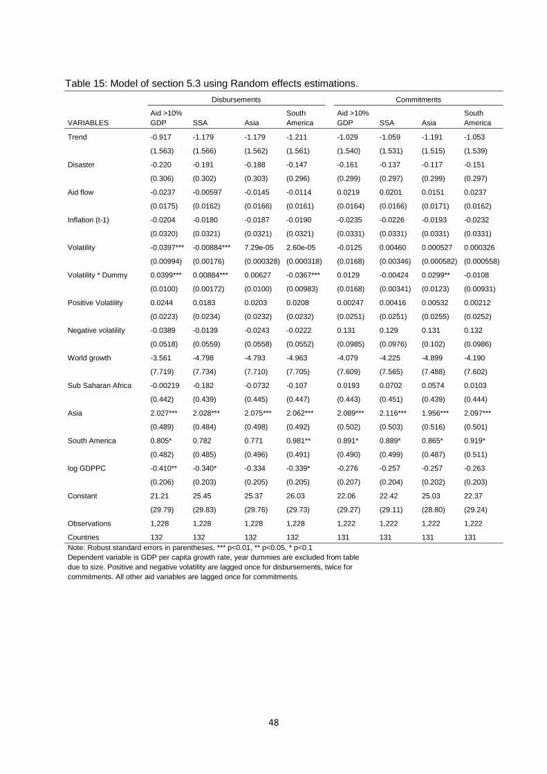
48

Table 15: Model of section 5.3 using Random effects estimations.

Disbursements Commitments

VARIABLES

Aid >10%

GDP SSA Asia

South

America

Aid >10%

GDP SSA Asia

South

America

Trend -0.917 -1.179 -1.179 -1.211 -1.029 -1.059 -1.191 -1.053

(1.563) (1.566) (1.562) (1.561)

(1.540) (1.531) (1.515) (1.539)

Disaster -0.220 -0.191 -0.188 -0.147

-0.161 -0.137 -0.117 -0.151

(0.306) (0.302) (0.303) (0.296)

(0.299) (0.297) (0.299) (0.297)

Aid flow -0.0237 -0.00597 -0.0145 -0.0114

0.0219 0.0201 0.0151 0.0237

(0.0175) (0.0162) (0.0166) (0.0161)

(0.0164) (0.0166) (0.0171) (0.0162)

Inflation (t-1) -0.0204 -0.0180 -0.0187 -0.0190

-0.0235 -0.0226 -0.0193 -0.0232

(0.0320) (0.0321) (0.0321) (0.0321)

(0.0331) (0.0331) (0.0331) (0.0331)

Volatility -0.0397*** -0.00884*** 7.29e-05 2.60e-05

-0.0125 0.00460 0.000527 0.000326

(0.00994) (0.00176) (0.000328) (0.000318)

(0.0168) (0.00346) (0.000582) (0.000558)

Volatility * Dummy 0.0399*** 0.00884*** 0.00627 -0.0367***

0.0129 -0.00424 0.0299** -0.0108

(0.0100) (0.00172) (0.0100) (0.00983)

(0.0168) (0.00341) (0.0123) (0.00931)

Positive Volatility 0.0244 0.0183 0.0203 0.0208

0.00247 0.00416 0.00532 0.00212

(0.0223) (0.0234) (0.0232) (0.0232)

(0.0251) (0.0251) (0.0255) (0.0252)

Negative volatility -0.0389 -0.0139 -0.0243 -0.0222

0.131 0.129 0.131 0.132

(0.0518) (0.0559) (0.0558) (0.0552)

(0.0985) (0.0976) (0.102) (0.0986)

World growth -3.561 -4.798 -4.793 -4.963

-4.079 -4.225 -4.899 -4.190

(7.719) (7.734) (7.710) (7.705)

(7.609) (7.565) (7.488) (7.602)

Sub Saharan Africa -0.00219 -0.182 -0.0732 -0.107

0.0193 0.0702 0.0574 0.0103

(0.442) (0.439) (0.445) (0.447)

(0.443) (0.451) (0.439) (0.444)

Asia 2.027*** 2.028*** 2.075*** 2.062***

2.089*** 2.116*** 1.956*** 2.097***

(0.489) (0.484) (0.498) (0.492)

(0.502) (0.503) (0.516) (0.501)

South America 0.805* 0.782 0.771 0.981**

0.891* 0.889* 0.865* 0.919*

(0.482) (0.485) (0.496) (0.491)

(0.490) (0.499) (0.487) (0.511)

log GDPPC -0.410** -0.340* -0.334 -0.339*

-0.276 -0.257 -0.257 -0.263

(0.206) (0.203) (0.205) (0.205)

(0.207) (0.204) (0.202) (0.203)

Constant 21.21 25.45 25.37 26.03

22.06 22.42 25.03 22.37

(29.79) (29.83) (29.76) (29.73)

(29.27) (29.11) (28.80) (29.24)

Observations 1,228 1,228 1,228 1,228

1,222 1,222 1,222 1,222

Countries 132 132 132 132

131 131 131 131

Note: Robust standard errors in parentheses, *** p<0.01, ** p<0.05, * p<0.1

Dependent variable is GDP per capita growth rate, year dummies are excluded from table

due to size. Positive and negative volatility are lagged once for disbursements, twice for

commitments. All other aid variables are lagged once for commitments.

49

Table 16: Model of section 5.3 using fixed effects estimations

Disbursements Commitments

VARIABLES

Aid >10%

GDP SSA Asia

South

America

Aid >10%

GDP SSA Asia

South

America

Trend 0.243 0.0905 0.0624 0.107

0.301 0.340 0.166 0.322

(1.479) (1.479) (1.478) (1.478)

(1.445) (1.425) (1.427) (1.444)

Disaster -0.406 -0.411 -0.396 -0.334

-0.384 -0.360 -0.394 -0.391

(0.275) (0.276) (0.275) (0.258)

(0.278) (0.275) (0.276) (0.277)

Aid flow -0.0241 -0.00569 -0.0134 -0.00935

0.0340 0.0212 0.0290 0.0309

(0.0199) (0.0192) (0.0189) (0.0181)

(0.0250) (0.0245) (0.0240) (0.0242)

Inflation (t-1) -0.0748** -0.0745** -0.0734** -0.0728**

-0.0841** -0.0814** -0.0797** -0.0842**

(0.0347) (0.0349) (0.0348) (0.0346)

(0.0370) (0.0370) (0.0368) (0.0370)

Volatility -0.0298*** -0.00734*** -1.35e-05 -7.10e-05

0.0121 0.00985** -0.000216 -0.000246

(0.00922) (0.00195) (0.000306) (0.000295)

(0.0178) (0.00382) (0.000553) (0.000577)

Volatility*Dummy 0.0299*** 0.00726*** -0.00905 -0.0420***

-0.0124 -0.0100*** 0.0355 0.00511

(0.00931) (0.00191) (0.00992) (0.0119)

(0.0179) (0.00383) (0.0221) (0.00983)

Positive volatility 0.0287 0.0244 0.0256 0.0262

-0.00433 0.00151 -0.00282 -0.00456

(0.0219) (0.0226) (0.0225) (0.0224)

(0.0278) (0.0275) (0.0287) (0.0277)

Negative volatility -0.0716* -0.0534 -0.0604 -0.0589

0.109 0.0996 0.113 0.109

(0.0383) (0.0380) (0.0395) (0.0383)

(0.0900) (0.0871) (0.0925) (0.0905)

World growth -0.0959 -0.792 -0.929 -0.772

0.304 0.466 -0.370 0.400

(7.210) (7.221) (7.212) (7.207)

(7.053) (6.970) (6.988) (7.054)

log GDPPC -5.088*** -5.001** -5.006** -5.104***

-4.834** -4.908** -4.812** -4.862**

(1.928) (1.929) (1.927) (1.919)

(1.994) (1.976) (1.978) (1.984)

Constant 39.99 41.97 42.57 42.54

36.51 36.42 38.93 36.37

(30.54) (30.68) (30.66) (30.57)

(30.24) (30.03) (30.20) (30.28)

Observations 1,228 1,228 1,228 1,228

1,222 1,222 1,222 1,222

R-squared 0.099 0.099 0.097 0.101

0.099 0.101 0.101 0.099

Countries 132 132 132 132

131 131 131 131

Note: Robust and clustered standard errors in parentheses, *** p<0.01, ** p<0.05,

* p<0.1

Dependent variable is GDP per capita growth rate, year dummies are excluded from table

due to size. Positive and negative volatility are lagged once for disbursements, twice for

commitments. All other aid variables are lagged once for commitments.

50

Table 17: Estimations of model of section 5.4

Random Effects Fixed effects

VARIABLES No interaction

Aid > 10%

GDP

No interaction Aid > 10% GDP

Trend -1.210 -1.319 0.0790 -0.0229

(1.578) (1.601)

(1.476) (1.504)

Diaster -0.148 -0.125

-0.397 -0.396

(0.308) (0.311)

(0.275) (0.284)

Aid flows -0.00420 0.000487

-0.000672 -0.000855

(0.0180) (0.0182)

(0.0296) (0.0278)

Inflation (t-1) -0.0159 -0.0132

-0.0741** -0.0702**

(0.0321) (0.0318)

(0.0350) (0.0350)

Volatility 0.000265 0.000105

-1.04e-05 -0.000147

(0.000332) (0.000346)

(0.000290) (0.000315)

Predictability -0.0316 -0.202**

-0.0163 -0.191**

(0.0210) (0.0892)

(0.0324) (0.0951)

Predictability*Aid dependency

0.180**

0.187**

(0.0909)

(0.0944)

Positive volatility (t-1) -0.00212 0.00159

0.0170 0.0199

(0.0198) (0.0192)

(0.0160) (0.0154)

Negative volatility (t-1) -0.0200 -0.0219

-0.0671 -0.0610

(0.0597) (0.0570)

(0.0502) (0.0476)

World growth -4.941 -5.514

-0.825 -1.372

(7.791) (7.897)

(7.200) (7.340)

Sub Sahara Africa -0.0189 0.00296

(0.443) (0.436)

Asia 2.088*** 2.061***

(0.492) (0.490)

South America 0.798 0.801

(0.499) (0.508)

log GDPPC -0.273 -0.203

-4.926** -4.887**

(0.213) (0.214)

(1.957) (1.947)

Constant 25.35 26.80

41.50 43.10

(30.09) (30.47)

(30.76) (31.22)

Observations 1,228 1,228

1,228 1,228

R-squared

0.098 0.101

Countries 132 132

132 132

Note: Robust standard errors in parentheses, *** p<0.01, ** p<0.05, * p<0.1

Dependent variable is GDP per capita growth rate. Year dummies excluded from table due to size.

Standard errors are clustered and robust for fixed effects.

51

Table 18: Social infrastructure and services aid and its effect on death rate and school

completion, random effects. Section 6.1

VARIABLES Death rate School completion

Disbursement 0.000157

-0.0185**

(0.00196)

(0.00752)

Positive volatility 0.00191

0.0117

(0.00190)

(0.00871)

Negative volatility -0.00452**

0.0257**

(0.00209)

(0.0122)

Commitment (t-1)

-0.00435*

-0.0288***

(0.00242)

(0.0103)

Positive volatility (t-1)

0.00689***

0.0255**

(0.00230)

(0.0108)

Negative volatility (t-1)

0.00111

0.0350**

(0.00276)

(0.0145)

Constant 2.130*** 2.130***

3.897*** 3.987***

(0.0388) (0.0393)

(0.0651) (0.0639)

Observations 1,609 1,478

950 877

Countries 142 141

130 129

Note: Robust standard errors in parentheses, *** p<0.01, ** p<0.05, * p<0.1

Year dummies are excluded in the table because of size

Table 19: Social infrastructure and services aid and its effect on death rate and school

completion, country fixed effects. Section 6.1

VARIABLES Death rate School completion

Disbursement -3.38e-05

-0.0132*

(0.00196)

(0.00690)

Positive volatility 0.00213

0.00683

(0.00190)

(0.00802)

Negative volatility -0.00446**

0.0207*

(0.00210)

(0.0118)

Commitment (t-1)

-0.00467*

-0.0241**

(0.00249)

(0.0112)

Positive volatility (t-1)

0.00729***

0.0198*

(0.00239)

(0.0117)

Negative volatility (t-1)

0.00122

0.0327**

(0.00280)

(0.0152)

Constant 2.145*** 2.145***

3.896*** 3.977***

(0.0103) (0.00924)

(0.0273) (0.0332)

Observations 1,609 1,478

950 877

R-squared 0.313 0.314

0.341 0.304

Countries 142 141

130 129

Note: Clustered and robust standard errors in parentheses, *** p<0.01, ** p<0.05, * p<0.1

Year dummies are excluded in the table because of size

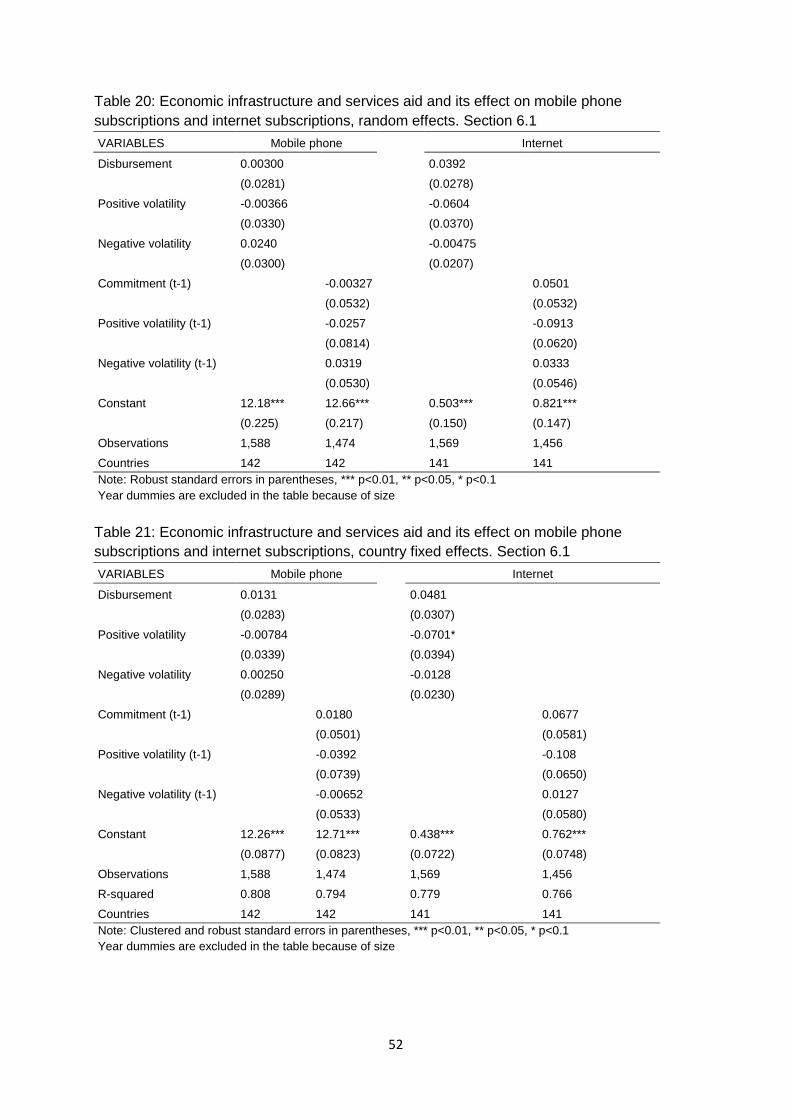
52

Table 20: Economic infrastructure and services aid and its effect on mobile phone

subscriptions and internet subscriptions, random effects. Section 6.1

VARIABLES Mobile phone Internet

Disbursement 0.00300

0.0392

(0.0281)

(0.0278)

Positive volatility -0.00366

-0.0604

(0.0330)

(0.0370)

Negative volatility 0.0240

-0.00475

(0.0300)

(0.0207)

Commitment (t-1)

-0.00327

0.0501

(0.0532)

(0.0532)

Positive volatility (t-1)

-0.0257

-0.0913

(0.0814)

(0.0620)

Negative volatility (t-1) 0.0319

0.0333

(0.0530)

(0.0546)

Constant 12.18*** 12.66***

0.503*** 0.821***

(0.225) (0.217)

(0.150) (0.147)

Observations 1,588 1,474

1,569 1,456

Countries 142 142

141 141

Note: Robust standard errors in parentheses, *** p<0.01, ** p<0.05, * p<0.1

Year dummies are excluded in the table because of size

Table 21: Economic infrastructure and services aid and its effect on mobile phone

subscriptions and internet subscriptions, country fixed effects. Section 6.1

VARIABLES Mobile phone Internet

Disbursement 0.0131

0.0481

(0.0283)

(0.0307)

Positive volatility -0.00784

-0.0701*

(0.0339)

(0.0394)

Negative volatility 0.00250

-0.0128

(0.0289)

(0.0230)

Commitment (t-1)

0.0180

0.0677

(0.0501)

(0.0581)

Positive volatility (t-1)

-0.0392

-0.108

(0.0739)

(0.0650)

Negative volatility (t-1) -0.00652

0.0127

(0.0533)

(0.0580)

Constant 12.26*** 12.71***

0.438*** 0.762***

(0.0877) (0.0823)

(0.0722) (0.0748)

Observations 1,588 1,474

1,569 1,456

R-squared 0.808 0.794

0.779 0.766

Countries 142 142

141 141

Note: Clustered and robust standard errors in parentheses, *** p<0.01, ** p<0.05, * p<0.1

Year dummies are excluded in the table because of size

53

Table 22: Models using different aid sectors and their effects on relevant microeconomic

indicators, random effects estimations. Section 6.1

Production sector Multi-sector Humanitarian

VARIABLES

Manufacturing

value added (%of

GDP)

CO2 emissions (log)

Death rate (log)

Disbursements 0.616 -0.000299 0.00929***

(0.538)

(0.00709)

(0.00241)

Disbursement

volatility (t-1, +) -0.655

-0.00737

-0.00772**

(0.683)

(0.0158)

(0.00307)

Disbursement

volatility (t-1, -) -0.546*

0.00888

-0.0109***

(0.322)

(0.0191)

(0.00386)

Commitments (t-1)

0.0462

-0.000370

0.00600

(0.206)

(0.00778)

(0.00479)

Commitment

volatility (t-1, +)

-0.192

-0.00350

-0.00223

(0.389)

(0.0191)

(0.00529)

Commitment

volatility (t-1, -)

0.0581

-0.00126

-0.0111*

(0.149)

(0.00907)

(0.00631)

Constant 12.61*** 12.99***

-0.463*** -0.450***

2.148*** 2.140***

(0.656) (0.653)

(0.0761) (0.0753)

(0.0383) (0.0377)

Observations 1,424 1,303

1,207 1,069

1,486 1,375

Number of country 133 132

140 140

139 139

Note: Robust standard errors in parentheses, *** p<0.01, ** p<0.05, *

p<0.1

Year dummies are excluded in the table because of size

54

Table 23: Models using different aid sectors and their effects on relevant microeconomic

indicators, country fixed effects estimations. Section 6.1

Production sector Multi-sector Humanitarian

VARIABLES Manufacturing value added

(% of GDP) CO2 emmisions

Death rate

Disbursements 0.694 9.00e-05 0.00908***

(0.542)

(0.00714)

(0.00245)

Disbursement volatility

(+) -0.707

-0.00732

-0.00749**

(0.685)

(0.0157)

(0.00308)

Disbursement volatility

(-) -0.675**

0.00812

-0.0107***

(0.329)

(0.0189)

(0.00388)

Commitments (t-1)

0.0845

0.000387

0.00558

(0.217)

(0.00786)

(0.00485)

Commitment volatility

(t-1, +) -0.232

-0.00160

-0.00175

(0.402)

(0.0195)

(0.00534)

Commitment volatility

(t-1, -) 0.0220

-0.00206

-0.0108*

(0.165)

(0.00877)

(0.00633)

Constant 12.83*** 13.20***

-0.470*** -0.458***

2.163*** 2.153***

(0.272) (0.193)

(0.0161) (0.0152)

(0.00942) (0.00884)

Observations 1,424 1,303

1,207 1,069

1,486 1,375

R-squared 0.164 0.149

0.033 0.035

0.358 0.338

Number of countries 133 132 140 140 139 139

Note: Clustered and robust standard errors in parentheses, *** p<0.01, **

p<0.05, * p<0.1

Year dummies are excluded in the table because of size

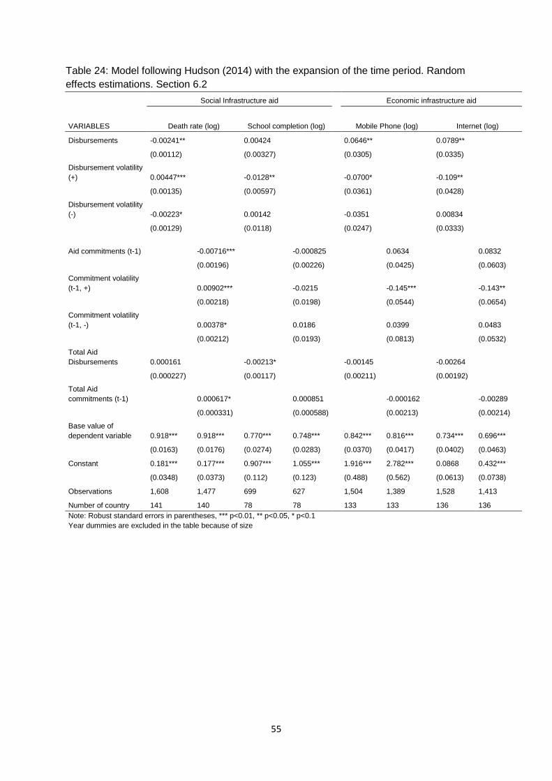
55

Table 24: Model following Hudson (2014) with the expansion of the time period. Random

effects estimations. Section 6.2

Social Infrastructure aid Economic infrastructure aid

VARIABLES Death rate (log) School completion (log)

Mobile Phone (log) Internet (log)

Disbursements -0.00241** 0.00424 0.0646** 0.0789**

(0.00112)

(0.00327)

(0.0305)

(0.0335)

Disbursement volatility

(+) 0.00447*** -0.0128**

-0.0700*

-0.109**

(0.00135)

(0.00597)

(0.0361)

(0.0428)

Disbursement volatility

(-) -0.00223*

0.00142

-0.0351

0.00834

(0.00129)

(0.0118)

(0.0247)

(0.0333)

Aid commitments (t-1)

-0.00716*** -0.000825

0.0634

0.0832

(0.00196)

(0.00226)

(0.0425)

(0.0603)

Commitment volatility

(t-1, +)

0.00902***

-0.0215

-0.145***

-0.143**

(0.00218)

(0.0198)

(0.0544)

(0.0654)

Commitment volatility

(t-1, -)

0.00378*

0.0186

0.0399

0.0483

(0.00212)

(0.0193)

(0.0813)

(0.0532)

Total Aid

Disbursements 0.000161

-0.00213*

-0.00145

-0.00264

(0.000227)

(0.00117)

(0.00211)

(0.00192)

Total Aid

commitments (t-1)

0.000617*

0.000851

-0.000162

-0.00289

(0.000331)

(0.000588)

(0.00213)

(0.00214)

Base value of

dependent variable 0.918*** 0.918*** 0.770*** 0.748***

0.842*** 0.816*** 0.734*** 0.696***

(0.0163) (0.0176) (0.0274) (0.0283)

(0.0370) (0.0417) (0.0402) (0.0463)

Constant 0.181*** 0.177*** 0.907*** 1.055***

1.916*** 2.782*** 0.0868 0.432***

(0.0348) (0.0373) (0.112) (0.123)

(0.488) (0.562) (0.0613) (0.0738)

Observations 1,608 1,477 699 627

1,504 1,389 1,528 1,413

Number of country 141 140 78 78

133 133 136 136

Note: Robust standard errors in parentheses, *** p<0.01, ** p<0.05, * p<0.1

Year dummies are excluded in the table because of size

56

Table 25: Model following Hudson (2014) with the expansion of the time period. Country

fixed effects estimations. Section 6.2

Social Infrastructure aid Economic infrastructure aid

VARIABLES Death rate (log)

School completion

(log)

Mobile Phone (log) Internet (log)

Disbursements -0.000412

-0.00344

0.0552*

0.0766**

(0.00173)

(0.00717)

(0.0309)

(0.0336)

Disbursement volatility (+) 0.00247

-0.00269

-0.0556

-0.102**

(0.00174)

(0.00689)

(0.0359)

(0.0411)

Disbursement volatility (-) -0.00427** 0.00875

-0.0405

-0.00148

(0.00200)

(0.0146)

(0.0278)

(0.0382)

Aid commitments (t-1)

-0.00614**

-0.0211*

0.0544

0.0836

(0.00247)

(0.0116)

(0.0434)

(0.0607)

Commitment volatility (t-1,

+)

0.00779***

0.00359

-0.130**

-0.136**

(0.00248)

(0.0163)

(0.0549)

(0.0650)

Commitment volatility (t-1,

-)

0.00285

0.0426

0.0417

0.0358

(0.00282)

(0.0265)

(0.0880)

(0.0615)

Total Aid Disbursements 0.000208

-0.00336***

-0.00194

-0.00205

(0.000262)

(0.00120)

(0.00208) (0.00196)

Total Aid commitments (t-

1)

0.000680*

0.000270

-0.000898

-0.00280

(0.000353)

(0.000674)

(0.00214)

(0.00219)

Base value of dependent

variable - - - -

- - - -

Constant 2.145*** 2.144*** 3.941*** 4.025***

12.38*** 12.92*** 0.433*** 0.772***

(0.0106) (0.00988) (0.0238) (0.0308)

(0.0896) (0.0767) (0.0765) (0.0768)

Observations 1,608 1,477 699 627

1,504 1,389 1,528 1,413

R-squared 0.314 0.318 0.348 0.281

0.816 0.803 0.783 0.770

Number of country 141 140 78 78

133 133 136 136

Note: Clustered and robust standard errors in parentheses, *** p<0.01, **

p<0.05, * p<0.1

Year dummies are excluded in the table because of size