Stock Market Volatility and Learning∗

Klaus Adam Albert Marcet Juan Pablo Nicolini

August 14, 2007

Abstract

Introducing bounded rationality into a standard consumption basedasset pricing model with a representative agent and time separable pref-erences strongly improves empirical performance. Learning causes mo-mentum and mean reversion of returns and thereby excess volatility, per-sistence of price-dividend ratios, long-horizon return predictability and arisk premium, as in the habit model of Campbell and Cochrane (1999),but for lower risk aversion. This is obtained, although we restrict con-sideration to learning schemes that imply only small deviations from fullrationality. The findings are robust to the particular learning rule usedand the value chosen for the single free parameter introduced by learn-ing, provided agents forecast future stock prices using past informationon prices.

JEL Class. No.: G12, D84

∗Thanks go to Luca Dedola and Jaume Ventura for interesting comments and suggestions.We particularly thank Phillip Weil for a very interesting discussion. Davide Debortoli hassupported us with outstanding research assistance. Marcet acknowledges support from CIRIT(Generalitat de Catalunya), DGES (Ministry of Education and Science), CREI, the BarcelonaEconomics program of XREA and the Wim Duisenberg fellowship from the European CentralBank. The views expressed herein are solely those of the authors and do not necessarilyreflect the views of the European Central Bank. Author contacts: Klaus Adam (EuropeanCentral Bank and CEPR) klaus.adam@ecb.int; Albert Marcet (Institut d’Analisi EconomicaCSIC, Universitat Pompeu Fabra) albert.marcet@upf.edu; Juan Pablo Nicolini (UniversidadTorcuato di Tella) juanpa@utdt.edu.

1

"Investors, their confidence and expectations buoyed by past price increases,bid up speculative prices further, thereby enticing more investors to do thesame, so that the cycle repeats again and again, .. "

Irrational Exuberance, Shiller (2005, p.56)

1 IntroductionThe purpose of this paper is to show that a very simple asset pricing model isable to reproduce a variety of stylized facts if one allows for small departuresfrom rationality. This result is somehow remarkable, since the literature in em-pirical finance had great difficulties in developing dynamic equilibrium rationalexpectations models accounting for all the facts we consider.Our model is based on the representative agent time-separable utility endow-

ment economy developed by Lucas (1978). It is well known that the implicationsof this model under rational expectations are at odds with basic asset pricingobservations: the price dividend ratio is too volatile and persistent, stock re-turns are too volatile and should not be negatively related to the price dividendratio in the long run, and the risk premium is too high. Our learning modelintroduces just one additional free parameter into Lucas’ framework and quan-titatively accounts for all these observations. Since the learning model reducesto the rational expectations model if the additional parameter is set to zero andsince this parameter is close to zero throughout the paper, we consider the learn-ing model to represent only a small departure from rationality. Nevertheless,the behavior of equilibrium prices differs considerably from the one obtainedunder rational expectations, implying that the asset pricing implications of thestandard model are not robust to small departures from rationality. As we doc-ument, this non-robustness is empirically encouraging, i.e., the model matchesthe data much better if this small departure from rationality is allowed for.A very large body of literature has documented that stock prices exhibit

movements that are very hard to reproduce within the realm of rational expec-tations and Lucas’ tree model has been extended in a variety of directions toimprove its empirical performance. After several years of research, Campbelland Cochrane (1999) succeeded in reproducing all the facts, albeit at the cost ofimposing complicated non-time-separabilities in preferences and high effectivedegrees of risk aversion. Our model retains simplicity and moderate curvaturein utility, but instead deviates from full rationality.The behavioral finance literature tried to understand the decision making

process of individual investors by means of surveys, experiments and microevidence, exploring the intersection between economics and psychology. Oneof the main themes of this literature was to test the rationality hypothesis inasset markets, see Shiller (2005) for a non-technical summary. We borrow some

2

of the economic intuition from this literature, but follow a different modelingapproach: we aim for a model that is as close as possible to the original Lucastree model, with agents who are quasi-rational and formulate forecasts usingstatistical models that imply only small departures from rationality.In the baseline learning model, we assume agents form their expectations

regarding future stock prices with the most standard scheme used in the lit-erature: ordinary least squares learning (OLS).1 This rule has the propertythat in the long run the equilibrium converges to rational expectations, but inthe model this process takes a very long time, and the dynamics generated bylearning along the transition cause prices to be very different from the rationalexpectations (RE) prices. This difference occurs for the following reasons: ifexpectations about stock price growth have increased, the actual growth rate ofprices has a tendency to increase beyond the fundamental growth rate, therebyreinforcing the initial belief of higher stock price growth. Learning thus imparts‘momentum’ on stock prices and beliefs and produces large and sustained devi-ations of the price dividend ratio from its mean, as can be observed in the data.The model thus displays something like the ‘naturally occurring Ponzi schemes’described in Shiller’s opening quote above.As we mentioned, OLS is the most standard assumption to model the evolu-

tion of expectations functions in the learning literature and its limiting proper-ties have been used extensively as a stability criterion to justify or discard REequilibria. Yet, models of learning are still not commonly used to explain dataor for policy analysis.2 It is still the standard view in the economics researchliterature that models of learning introduce too many degrees of freedom, sothat it is easy to find a learning scheme that matches whatever observation onedesires. One can deal with this important methodological issue in two ways:first, by using a learning scheme with as few free parameters as possible, andsecond, by imposing restrictions on the parameters of the learning scheme toonly allow for small departures of rationality.3 These considerations promptedus to use an off-the-shelf learning scheme (OLS) that has only one free parame-ter. In addition, in the model at hand, OLS is the best estimator in the longrun, and to make the departure form rationality during the transition small, weassume that initial beliefs are at the rational expectations equilibrium, and thatagents have very strong - but less than complete - confidence in these initialbeliefs, as we explain in detail in the main text.Models of learning have been used before to explain some aspects of asset

price behavior. Timmermann (1993, 1996), Brennan and Xia (2001) and Cogleyand Sargent (2006) show that Bayesian learning can help explain various aspectsof stock prices. These authors assume that agents learn about the dividend

1We show that results are robust to using other standard learning rules.2We will mention some exceptions along the paper.3Marcet and Nicolini (2005) dealt with this issue by imposing bounds on the size of the

mistakes agents can make in equilibrium. These bounds imposed discipline both on the typeof learning rule and on the exact value of the parameters in the learning rule. For the presentmodel we show that results are very robust to both the learning rule and the exact value ofthe single learning parameter.

3

process and use the Bayesian posterior on the dividend process to estimate thediscounted sum of dividends that would determine the stock price under RE.Therefore, while the beliefs of agents influence the market outcomes, agents’beliefs remain unaffected by market outcomes because agents learn only aboutan exogenous dividend process. In the language of stochastic control, thesemodels are not self-referential. In the language of Shiller, these models cannot give rise to ‘naturally occurring Ponzi schemes’. In contrast, we largelyabstract from learning about the dividend process and consider learning on thefuture stock price using past observations of price, so that beliefs and prices aremutually determined. It is precisely the learning about future stock price growthand its self-referential nature that imparts the momentum to expectations and,therefore, is key in explaining the data.4

Other related papers by Bullard and Duffy (2001) and Brock and Hommes(1998) show that learning dynamics can converge to complicated attractors, ifthe RE equilibrium is unstable under learning dynamics.5 Branch and Evans(2006) study a model where agents’ expectations switch depending on whichof the available forecast models is performing best. By comparison, we look atlearning about the stock price growth rate, we address more closely the data,and we do so in a model where the rational expectations equilibrium is stableunder learning dynamics, so the departure from RE behavior occurs only alonga transition related to the sample size of the observed data. Also related isCárceles-Poveda and Giannitsarou (2006) who assume that agents know themean stock price and learn only about the deviations from the mean; they findthat the presence of learning does then not significantly alter the behavior ofasset prices.6

The paper is organized as follows. Section 2 presents the stylized facts we fo-cus on and the basic features of the underlying asset pricing model, showing thatthis model cannot explain the facts under the rational expectations hypothesis.In section 3 we take the simplest risk neutral model and assume instead thatagents learn to forecast the growth rate of prices. We show that such a modelcan qualitatively deliver all the considered asset pricing facts and that learningconverges to rational expectations. We also explain how the deviations fromrational expectations can be made arbitrarily small. In Section 4 we presentthe baseline learning model with risk aversion and the baseline calibration pro-cedure. We also explain why we choose to calibrate the model parameters ina slightly different way than in standard calibration exercises. Section 5 showsthat the baseline model can quantitatively reproduce all the facts discussed insection 2. The robustness of our findings to various assumptions about themodel, the learning rule, or the calibration procedure is illustrated in section 6.

4Timmerman (1996) analyzes in one setting also a self-referential model, but one in whichagents use dividends to predict future price. He finds that this form of self-referntial learningdelivers lower volatility than settings with learning about the dividend process. It is thuscrucial for our results that agents use information on past price behavior to predict futureprice.

5 Stability under learning dynamics is defined in Marcet and Sargent (1989).6Cecchetti, Lam, and Mark (2000) determine the misspecification in beliefs about future

consumption growth required to match the equity premium and other moments of asset prices.

4

Readers interested in obtaining a glimpse of the quantitative performanceof the baseline learning model may - after reading section 2 - directly jump totable 4 in section 5.

2 FactsThis section describes stylized facts of U.S. stock price data and explains why itproved difficult to reproduce them using standard rational expectations models.The facts presented in this section have been extensively documented in theliterature. We reproduce them here as a point of reference for our quantitativeexercise in the latter part of the paper and using a single and updated data set.7

It is useful to start looking at the data through the lens of a simple dynamicstochastic endowment economy. Let Dt be the dividend of an inelastically sup-plied asset in period t, evolving according to

Dt

Dt−1= aεt (1)

where log εt ∼ N(− s2

2 , s2) is i.i.d. and a ≥ 1 the expected growth rate of

dividends.8 Let the preferences of a representative consumer-investor be givenby

E0

∞Xt=0

δtU (Ct)

where Ct is consumption at time t, δ the discount factor and U (·) strictlyincreasing and concave. With St denoting the end-of-period t stock holdings,the budget constraint is

Pt St + Ct = (Pt +Dt)St−1,

where Pt is the real price of the asset. In an equilibrium with rational expecta-tions, the asset price must satisfy the consumer’s first order condition evaluatedat Ct = Dt

Pt = δEt

∙U(Dt+1)

U(Dt)(Pt+1 +Dt+1)

¸(2)

which defines a mapping from the exogenous dividend process to the stochasticprocess of prices.9 The nature of this mapping obviously depends on the waythe intertemporal marginal rate of substitution moves with consumption. Forinstance, in the standard case of power preferences

U(Ct) =(Ct)

1−σ − 11− σ

7Details on the underlying data sources are provided in Appendix A.1.8As documented in Mankiw, Romer and Shapiro (1985) and Campbell (2003), this is a

reasonable first approximation to the empirical behavior of quarterly dividends in the U.S. Itis also the standard assumption in the literature.

9 In the data, consumption is much less volatile than dividends. This raises importantissues that will be discussed later in the paper.

5

0

100

200

300

400

1925 1930 1935 1940 1945 1950 1955 1960 1965 1970 1975 1980 1985 1990 1995 2000 2005

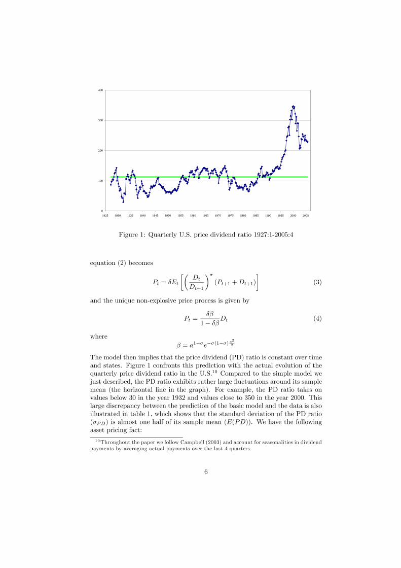
Figure 1: Quarterly U.S. price dividend ratio 1927:1-2005:4

equation (2) becomes

Pt = δEt

∙µDt

Dt+1

¶σ(Pt+1 +Dt+1)

¸(3)

and the unique non-explosive price process is given by

Pt =δβ

1− δβDt (4)

whereβ = a1−σe−σ(1−σ)

s2

2

The model then implies that the price dividend (PD) ratio is constant over timeand states. Figure 1 confronts this prediction with the actual evolution of thequarterly price dividend ratio in the U.S.10 Compared to the simple model wejust described, the PD ratio exhibits rather large fluctuations around its samplemean (the horizontal line in the graph). For example, the PD ratio takes onvalues below 30 in the year 1932 and values close to 350 in the year 2000. Thislarge discrepancy between the prediction of the basic model and the data is alsoillustrated in table 1, which shows that the standard deviation of the PD ratio(σPD) is almost one half of its sample mean (E(PD)). We have the followingasset pricing fact:

10Throughout the paper we follow Campbell (2003) and account for seasonalities in dividendpayments by averaging actual payments over the last 4 quarters.

6

• Fact 1: The PD ratio is very volatile.

It follows from equation (2) that matching the observed volatility of thePD ratio under rational expectation requires alternative preference specifica-tions. Indeed, maintaining the assumptions of i.i.d. dividend growth and of arepresentative agent, the behavior of the marginal rate of substitution is theonly degree of freedom left to the theorist. This explains the development of alarge and interesting literature exploring non-time-separability in consumptionor consumption habits. Introducing habit amounts to consider consumers whosepreferences are given by

E0

∞Xt=0

δt(Ct)1−σ − 11− σ

,

where Ct = H(Ct, Ct−1, Ct−2, ...) is a function of current and past consump-tion.11 A simple habit model has been studied by Abel (1990) who assumes

Ct =Ct

Cκt−1

with κ ∈ (0, 1).12 In this case, the asset price under rational expectations isPtDt

= A (aεt)κ(σ−1) (5)

for some constant A, which shows that this model can give rise to a volatilePD ratio. Yet, with εt being i.i.d. the PD ratio will display no autocorrelation,which is in stark contrast to the empirical evidence. As figure 1 illustrates, thePD ratio displays rather persistent deviations from its sample mean. Indeed,as table 1 shows, the quarterly autocoorelation of the PD ratio (ρPDt,PDt−1) isvery high. Therefore, this is the second fact we focus on:

• Fact 2. The PD ratio is persistent.

The previous observations suggest that matching the volatility and persis-tence of the PD ratio under rational expectations would require preferences thatgive rise to a volatile and persistent marginal rate of substitution. This is theavenue pursued in Campbell and Cochrane (1999) who engineer preferences thatcan match the behavior of the PD ratio we observe in Figure 1. Their speci-fication also helps in replicating the asset pricing facts mentioned later in thissection, as well as other facts not mentioned here.13 Their solution requires,however, imposing a very high degree of relative risk aversion and relies on arather complicated structure for the habit function H (·).1411We keep power utility for expositional purposes only.12 Importantly, the main purpose of Abel’s model was to generate an ‘equity premium’ - a

fact we discuss below - not to reproduce the behavior of the price dividend ratio.13They also match the pro-cyclical variation of stock prices and the counter-cyclical variation

of stock market volatility. We have not explored conditional moments in our learning model,see also the discussion at the end of this section.14The coefficient of relative risk aversion is 35 in steady state and higher still in states with

‘low surplus consumption ratios’.

7

In our model we maintain the assumption of standard time-separable con-sumption preferences with moderate degrees of risk aversion. Instead, we relaxthe rational expectations assumption by replacing the mathematical expectationin equation (2) by the most standard learning algorithm used in the literature.Persistence and volatility of the price dividend ratio will then be the result ofadjustments in beliefs that are induced by the learning process.Before getting into the details of our model, we want to mention three addi-

tional asset pricing facts about stock returns. These facts have received consid-erable attention in the literature and are qualitatively related to the behaviorof the PD ratio, as we discuss below.

• Fact 3. Stock returns are ‘excessively’ volatile.

Starting with the work of Shiller (1981) and LeRoy and Porter (1981) it hasbecome well-known that the volatility of the PD ratio is largely the result of largechanges in stock prices. Related to this is the observation that the volatility ofstock returns (σrs) in the data is much higher than the volatility of dividendgrowth (σ∆D/D), see table 1.15 The observed amount of return volatility hasbeen called ‘excessive’ mainly because the rational expectations model with timeseparable preferences predicts approximately identical volatilities. To see this,let rst denote the stock return

rst =Pt +Dt − Pt−1

Pt−1=

"PtDt+ 1

Pt−1Dt−1

#Dt

Dt−1− 1 (6)

and note that with time-separable preferences and i.i.d. dividend growth, thePD ratio is constant and the term in the square brackets above approximatelyequal to one.From equation (6) follows that excessive return volatility is qualitatively re-

lated to Fact 1 discussed above, as return volatility depends partly on the volatil-ity of the PD ratio.16 Yet, quantitatively return volatility also depends on thevolatility of dividend growth and - up to a linear approximation - on the firsttwo moments of the cross-correlogram between the PD ratio and the rate ofgrowth of dividends. Since the main contribution of the paper is to show theability of the learning model to account for the quantitative properties of thedata, we treat the volatility of returns as a separate asset pricing fact.

15This is not due to accounting for seasonalities in dividends by taking averages: stockreturns are also about three times as volatile as dividend growth at yearly frequency.16Cochrane (2005) provides a detailed derivation of the qualitative relationship between

facts 3 and 1 for i.i.d. dividend growth.

8

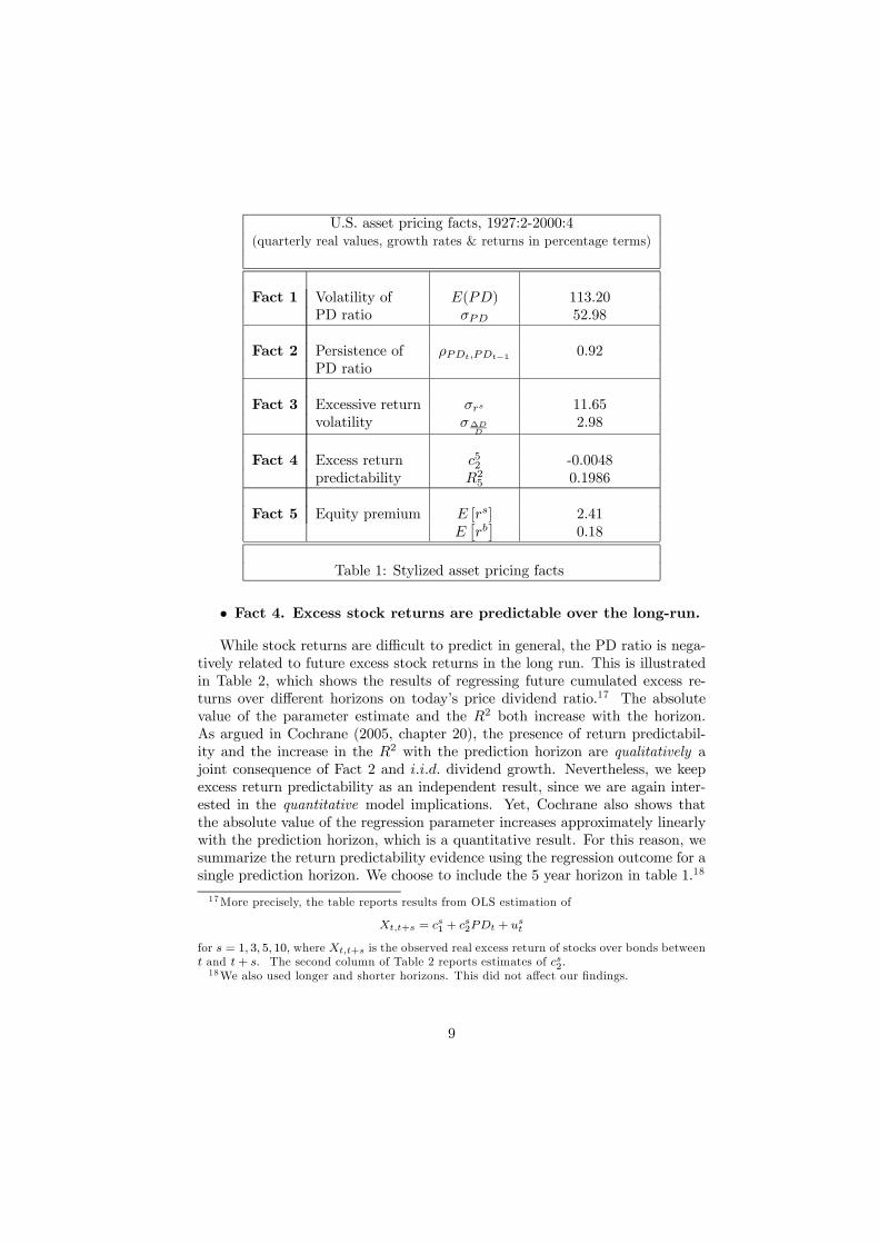
U.S. asset pricing facts, 1927:2-2000:4(quarterly real values, growth rates & returns in percentage terms)

Fact 1 Volatility of E(PD) 113.20PD ratio σPD 52.98

Fact 2 Persistence of ρPDt,PDt−1 0.92PD ratio

Fact 3 Excessive return σrs 11.65volatility σ∆D

D2.98

Fact 4 Excess return c52 -0.0048predictability R25 0.1986

Fact 5 Equity premium E [rs] 2.41E£rb¤

0.18

Table 1: Stylized asset pricing facts

• Fact 4. Excess stock returns are predictable over the long-run.

While stock returns are difficult to predict in general, the PD ratio is nega-tively related to future excess stock returns in the long run. This is illustratedin Table 2, which shows the results of regressing future cumulated excess re-turns over different horizons on today’s price dividend ratio.17 The absolutevalue of the parameter estimate and the R2 both increase with the horizon.As argued in Cochrane (2005, chapter 20), the presence of return predictabil-ity and the increase in the R2 with the prediction horizon are qualitatively ajoint consequence of Fact 2 and i.i.d. dividend growth. Nevertheless, we keepexcess return predictability as an independent result, since we are again inter-ested in the quantitative model implications. Yet, Cochrane also shows thatthe absolute value of the regression parameter increases approximately linearlywith the prediction horizon, which is a quantitative result. For this reason, wesummarize the return predictability evidence using the regression outcome for asingle prediction horizon. We choose to include the 5 year horizon in table 1.18

17More precisely, the table reports results from OLS estimation of

Xt,t+s = cs1 + cs2PDt + ust

for s = 1, 3, 5, 10, where Xt,t+s is the observed real excess return of stocks over bonds betweent and t+ s. The second column of Table 2 reports estimates of cs2.18We also used longer and shorter horizons. This did not affect our findings.

9

Years Coefficient on PD, cs1 R2

1 -0.0008 0.04383 -0.0023 0.11965 -0.0048 0.198610 -0.0219 0.3285

Table 2: Excess stock return predictability

• Fact 5. The equity premium puzzle.

Finally, and even though the emphasis of our paper is on moments of thePD ratio and stock returns, it is interesting to note that learning also improvesthe ability of the standard model to match the equity premium puzzle, i.e., theobservation that stock returns - averaged over long time spans and measured inreal terms - tend to be high relative to short-term real bond returns. The equitypremium puzzle is illustrated in table 1, which shows the average quarterly realreturn on bonds (E

¡rbt¢) being much lower than the corresponding return on

stocks (E (rst )).

Unlike Campbell and Cochrane (1999) we do not include in our list of factsany correlation between stock market data and real variables like consumptionor investment. In this sense, we follow more closely the literature in finance. Inour model, it is the learning scheme that delivers the movement in stock prices,even in a model with risk neutrality in which the marginal rate of substitutionis constant. This contrasts with the habit literature where the movement ofstock prices is obtained by modeling the way the observed stochastic processfor consumption generates movements in the marginal rate of substitution. Thelatter explains why the habit literature focuses on the relationship between par-ticularly low values of consumption and low stock prices. Since this mechanismdoes not play a significant role in our model, we abstract from these asset pricingfacts.

3 The risk neutral caseIn this section we analyze the simplest asset pricing model assuming risk neu-trality and time separable preferences (σ = 0 and Ct = Ct). The goal of thissection is to derive qualitative results and to show how the introduction of learn-ing improves the performance compared to a setting with rational expectations.Sections 4 and 5 present a formal quantitative model evaluation, extending theanalysis to risk-averse investors.With risk neutrality and rational expectations the model misses almost all

of the asset pricing facts described in the previous section:19 the PD ratio is19Since the RE model implies a constant PD ratio, it trivially has a ‘persistent’ PD ratio.

10

constant, stock returns are unforecastable (i.i.d.) and approximately as volatileas dividend growth, i.e., do not display excess volatility. In addition, thereis no equity premium. For these reasons, the risk-neutral model is particularlysuited to illustrate how the introduction of learning qualitatively improves modelperformance.The consumer has beliefs about future variables, these beliefs are summa-

rized in expectations denoted eE that we now allow to be less than fully rational.Under the assumptions of this section, equation (3) becomes20

Pt = δ eEt (Pt+1 +Dt+1) (7)

This asset pricing equation will be the focus of our analysis in this section.Some papers in the learning literature21 have studied stock prices when

agents formulate expectations about the discounted sum of all future dividendsand set

Pt = eEt

∞Xj=1

δjDt+j (8)

and the evaluation of the expectation is based on the Bayesian posterior distri-bution of the parameters in the dividend process. It is well known that underRE and some limiting condition on price growth the one-period ahead formula-tion of (7) is equivalent to the discounted sum expression for prices.22 However,under the standard learning rules used in the literature, this is not the case.If agents learn on the price according to (8), the posterior is about parameters

of an exogenous variable, i.e., the dividend process. Market prices do thennot influence expectations. As a result, learning in these papers is not self-referential and Bayesian beliefs are straightforward to formulate. Yet, this lackof feedback from market prices to expectations also limits the ability of themodel to generate interesting ‘data-like’ behavior. Here instead, we use theformulation in equation (7), where agents are assumed to have a forecast modelof next period’s price and dividend. They try to estimate the parameters of thisforecast model and will have to use data on stock prices to do so. Our point willbe that it is precisely when agents formulate expectations on prices to satisfy(7) that there is a large effect of learning and that many moments of the dataare better matched. It is in fact this self-referential nature of our model thatmakes it attractive in explaining the data.Focusing on equation (7) instead of (8) can be justified by a number of other

arguments based on principles. Informally, one can say that most participantsin the stock market care much more about the selling price of the stock than20This equation is similarly implied by many other models, for example, it can be interpreted

as a no-arbitrage condition in a model with risk-neutral investors or can be derived from anoverlapping generations model. All that is required is that investors formulate expectationsabout the future payoff Pt+1 + Dt+1 and for investors’ choice to be in equilibrium, today’sprice has to equal next period’s discounted expected payoff.21For example, Timmermann (1993, 1996), Brennan and Xia (2001), Cogley and Sargent

(2006).22More precisely, equivalence is obtained if Et [·] = Et [·] and if the no-rational-bubble

requirement limj→∞ δj EPt+j = 0 must hold.

11

about the discounted dividends. More formally, this would arise in a model withonly short-run investors.23 Also, the discounted sum formula implicitly assumesthat agents know perfectly the process for the market interest rate, therefore iteither assumes a lot of knowledge about interest rates on the part of the agentsor it ignores issues of learning about the interest rate.24 Because of these anda number of other reasons25 ,26 we conclude that our one-period formulation interms of prices is an interesting avenue to explore.

3.1 Analytical results

In this section we show that the introduction of learning changes qualitativelythe behavior of stock prices in the direction of matching the stylized facts de-scribed above. At this point we consider a wide class of learning schemes thatincludes the standard linear rules used in the literature; later on we will restrictattention to learning schemes that forecast well within the model.We first trivially rewrite the expectation of the agent by splitting the sum

in the expectation:Pt = δ eEt (Pt+1) + δ eEt (Dt+1) (9)

We assume that agents know how to formulate the conditional expectation of thedividend eEt (Dt+1) = aDt, which amounts to assuming that agents have rationalexpectations about the dividend process. This simplifies the discussion andhighlights the fact that it is learning about future prices that allows the modelto better match the data. Appendix A.4 shows that the pricing implications arevery similar if agents also learn how to forecast dividends.27

Agents are assumed to use a learning scheme in order to form a forecasteEt(Pt+1) based on past information. Equation (4) shows that under rational

23Allen, Morris and Shin (2006) also make this argument informally. It is possible to justifyit formally in an overlapping generations model. We do not pursue this further in this paper.24This point can be formalized in a model of heterogeneous agents where the market interest

rate is not equal to the discount factor of a single agent. The agent’s knowledge about his/herown discount factor does then not imply knowledge of the market interest rate. A Bayesianagent would have to formulate expectations about the interest rate also and the learningformula would have to be altered significantly.25 If the model is slightly misspecified and agents use robust forecasting rules the ‘law of

iterated expectations’, which is required to obtain the discounted sum, may not hold. Learningabout stock price is then likely to be a more robust formulation of expectations. Adam(2007) provides experimental evidence of the breakdown of the law of iterated expectationsin an experiment where agents become gradually aware that they use a possibly misspecifiedforecasting model.26 It is also worth noting that most applications of the discounted dividend formula do not

make a strict use of the principles of Bayesian learning. For example, Timmermann assumesthat agents form a posterior for the serial correlation of dividends ρ. Then prices satisfyPt =

∞j=1 δ

j EBayt (ρj) Dt where EBay

t is the expectation with the Bayesian posterior.Therefore, a strictly Bayesian agent would use the posterior distribution to form a different

expectation EBayt (ρj) for each j. Instead, he uses Pt =

∞j=1 δ

j EBayt (ρ)

jDt , where

EBayt (ρ) is the OLS estimate. This is a valuable simplification but, of course, it is not a fully

rational model.27 In section 6 we verify this also quantitatively in a model with learning about dividends

and prices.

12

expectations Et [Pt+1] = aPt. As we restrict our analysis to learning rules thatbehave close enough to rational expectations, we specify expectations underlearning as eEt [Pt+1] = βt Pt (10)

where βt > 0 denotes agents’ time t estimate of gross stock price growth. Forβt = a, learning agents beliefs are rational. Also, if over time agents’ beliefsconverge to the RE equilibrium (limt→∞ βt = a), investors will realize in thelong-run that they were correct in using the functional form (10). Yet, duringthe transition beliefs may deviate from rational ones.It remains to specify how agents update their beliefs βt. We consider the

following general learning mechanism

∆βt = ft

µPt−1Pt−2

− βt−1

¶(11)

for some exogenously chosen functions ft : R→ R with the property

ft(0) = 0

f 0t > 0

We thus assume beliefs to adjust in the direction of the last prediction error,i.e., agents revise beliefs upwards (downwards), if they underpredicted (over-predicted) stock price growth in the past.28 Arguably, a learning scheme thatviolates these conditions would appear quite unnatural. For technical reasons,we also need to assume that the functions ft are such that

0 < βt < δ−1 (12)

at all times. This rules out beliefs βt > δ−1 which would imply that expectedstock returns exceed the inverse of the discount factor, prompting the represen-tative agent to have an infinite demand for stocks at any stock price.Deriving quantitative and convergence results on learning will require spec-

ifying the learning scheme more explicitly. At this point, we show that the keyfeatures of the model emerge within this more general specification.

3.1.1 Stock prices under learning

Given the perceptions βt, the expectation function (10), and the assumption onperceived dividends, equation (9) implies that prices under learning satisfy

Pt =δaDt

1− δβt. (13)

28Note that βt is determined from observations up to period t − 1 only. The assumptionthat the current price does not enter in the formulation of the expectations is common in thelearning literature and is entertained for simplicity. Difficulties emerging with simultaneousinformation sets are discussed in Adam (2003).

13

Since βt and εt are independent, the previous equation implies that

V ar

µln

PtPt−1

¶= V ar

µln1− δβt−11− δβt

¶+ V ar

µln

Dt

Dt−1

¶, (14)

and shows that price growth under learning is more volatile than dividendgrowth. Clearly, this occurs because the volatility of beliefs adds to the volatilitygenerated by fundamentals. While this intuition is present in previous models oflearning, e.g., Timmermann (1993), it will be particular to our case that under

more specific learning schemes V ar³ln 1−δβt

1−δβt+1

´is very high and remains high

for a long time.Equation (13) shows that the beliefs βt are monotonically related to the the

PD ratio. One can thus understand the qualitative dynamics of the PD ratioby studying the belief dynamics. We now derive these dynamics.

PtPt−1

= T (βt,∆βt) εt (15)

where

T (β,∆β) ≡ a+aδ ∆β

1− δβ(16)

Substituting (15) in the law of motion for beliefs (11) and using also (13) showsthat the dynamics of βt (t ≥ 1) can be described as a function of the shocks εt(t ≥ 1), the initial conditions (D0, P−1), and the initial belief β0. Alternatively,the evolution of βt is described by a second order stochastic non-linear differenceequation

∆βt+1 = ft+1 (T (βt,∆βt)εt − βt) . (17)

This equation can not be solved analytically, but it is still possible to gainqualitative insights into the belief dynamics of the model. We do this in thenext section.

3.1.2 Deterministic dynamics

To discuss the dynamics of beliefs βt under learning, we simplify matters byconsidering the deterministic case in which εt ≡ 1. Equation (17) then simplifiesto

∆βt+1 = ft+1 (T (βt,∆βt)− βt) . (18)

We thus restrict attention to the endogenous stock price dynamics generated bythe learning mechanism rather than the dynamics induced by exogenous distur-bances. Equation (18) shows that beliefs are increasing whenever T (βt,∆βt) >β, i.e., whenever actual stock price growth exceeds expected stock price growth.Understanding the evolution of beliefs thus requires studying the T -mapping.We start by noting that the actual stock price growth implied by T depends

not only on the level of price growth expectations βt but also on the change4βt, and that this imparts momentum on the stock prices, leading to a feedbackbetween increases in expectations and increases in actual stock price growth:

14

Momentum: For all βt ∈ (0, δ−1)

T (βt,∆βt) > a if ∆βt > 0

T (βt,∆βt) < a if ∆βt < 0

Therefore, if agents arrived at the rational expectations belief βt = a frombelow (4βt > 0), the price growth generated by the learning model exceeds thefundamental growth rate a. Therefore,

∆βt+1 > 0 if βt = a and ∆βt > 0

Just because agents’ expectations have become more optimistic (in what a jour-nalist would perhaps call a ‘bullish’ market), the price growth in the markethas a tendency to be larger than fundamental growth. Since agents will use thishigher-than-fundamental stock price growth to update their beliefs in the nextperiod, βt+1 will tend to overshoot a, which will further reinforce the upwardtendency. Since beliefs are monotonically related to the PD ratio, see equation(13), there will be momentum the asset price, which could be interpreted asa ‘naturally arising Ponzi process’. Conversely, if βt = a in a bearish market(∆βt < 0), beliefs and prices display downward momentum, i.e., a tendency toundershoot the RE value.Stock prices and beliefs, however, can not stay at levels unjustified by fun-

damentals forever. Appendix A.2 proves that under some additional technicalassumptions we have

Mean reversion: For any η > 0 and t such that βt > a+η (βt < a− η), thereis a finite time t > t such that βt < a+ η (βt > a− η).

Since η can be chosen arbitrarily small, the previous statement shows thatbeliefs will eventually move back arbitrarily close to fundamentals or even moveto the ‘other side’ of fundamentals. This occurs even if agents’ beliefs are cur-rently far away from fundamentals. The monotone relationship between beliefsand the PD ratio then implies mean reverting behavior of the PD ratio.

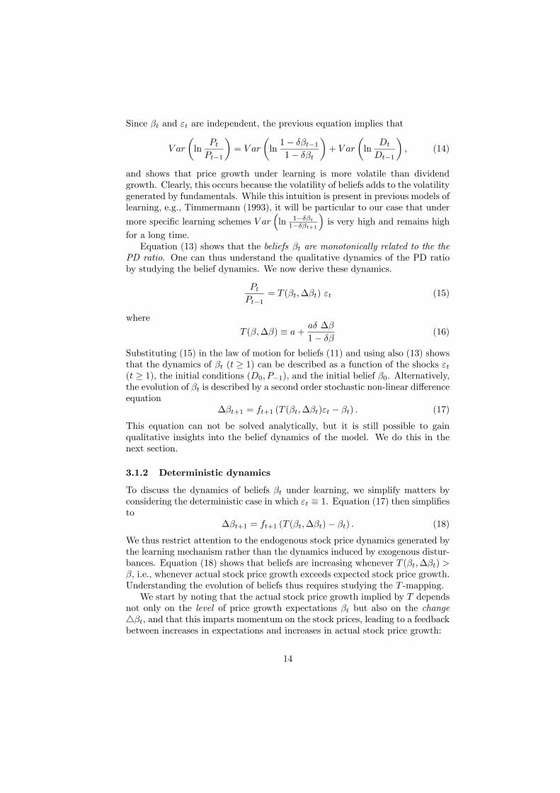
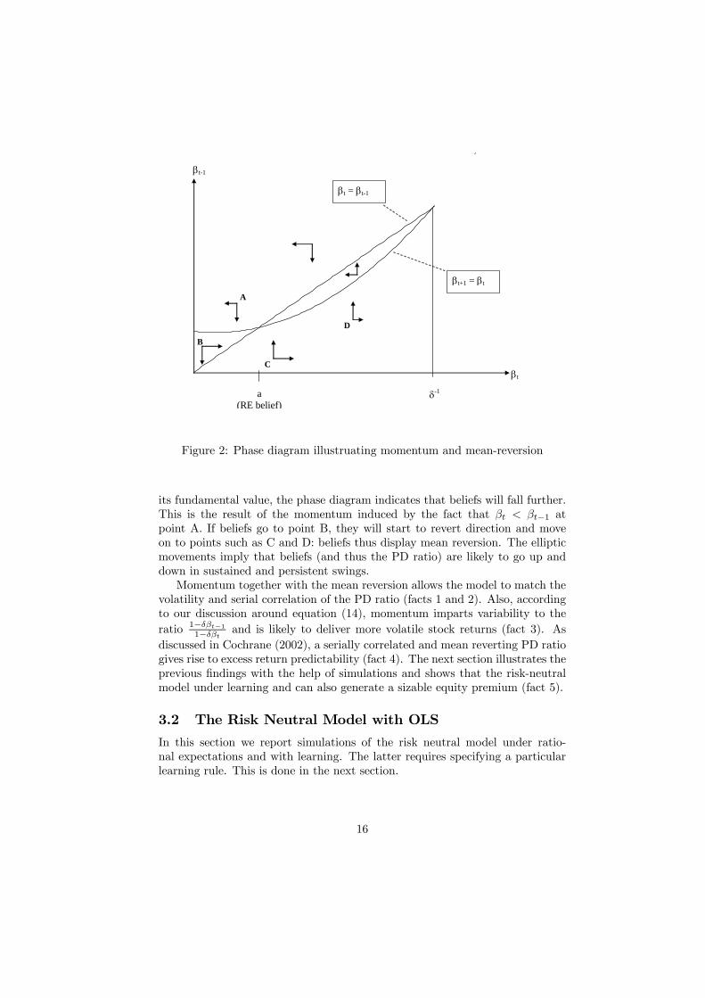
Figure 2 illustrates the momentum and mean reversion by depicting thephase diagram for the dynamics of the beliefs (βt, βt−1) implied by equation(18).29 The arrows in the figure thereby indicate the direction in which thedifference equation is going to move for any possible state (βt, βt−1) and the solidlines indicate the boundaries of these areas.30 Since we have a difference ratherthan a differential equation, we cannot plot the evolution of beliefs exactly.Nevertheless, the arrows suggest that the beliefs are likely to move in ellipsesaround the rational expectations equilibrium (βt, βt−1) = (a, a). Consider, forexample, point A in the diagram. Although at this point βt is already below

29Appendix A.3 explains the construction of the phase diagram.30The vertical solid line close to δ−1 is meant to illustrate the restriction β < δ−1 imposed

on the learning rule.

15

B

A

βt

βt-1

βt = βt-1

a (RE belief)

δ-1

βt+1 = βt

C

D

Figure 2: Phase diagram illustruating momentum and mean-reversion

its fundamental value, the phase diagram indicates that beliefs will fall further.This is the result of the momentum induced by the fact that βt < βt−1 atpoint A. If beliefs go to point B, they will start to revert direction and moveon to points such as C and D: beliefs thus display mean reversion. The ellipticmovements imply that beliefs (and thus the PD ratio) are likely to go up anddown in sustained and persistent swings.Momentum together with the mean reversion allows the model to match the

volatility and serial correlation of the PD ratio (facts 1 and 2). Also, accordingto our discussion around equation (14), momentum imparts variability to theratio 1−δβt−1

1−δβt and is likely to deliver more volatile stock returns (fact 3). Asdiscussed in Cochrane (2002), a serially correlated and mean reverting PD ratiogives rise to excess return predictability (fact 4). The next section illustrates theprevious findings with the help of simulations and shows that the risk-neutralmodel under learning and can also generate a sizable equity premium (fact 5).

3.2 The Risk Neutral Model with OLS

In this section we report simulations of the risk neutral model under ratio-nal expectations and with learning. The latter requires specifying a particularlearning rule. This is done in the next section.

16

3.2.1 The learning rule

We follow most empirical applications in the bounded rationality literature anduse the standard updating equation from the stochastic control literature

βt = βt−1 +1

αt

µPt−1Pt−2

− βt−1

¶(19)

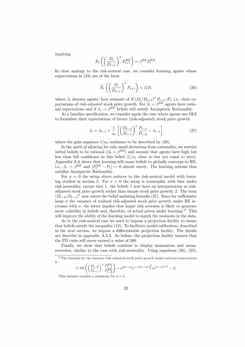
for all t ≥ 1, for a given sequence of αt, and a given initial belief β0 which isgiven outside the model.31 The sequence 1/αt is called the ‘gain’ sequence anddictates how strongly beliefs are updated in the direction of the last predictionerror. In this section, we assume the simplest possible specification:

1/αt = 1/ (αt−1 + 1) t ≥ 2 (20)

1/α1 ∈ [0, 1] given.

With these assumptions the model evolves as follows. In the first period, β0 de-termines the first price P0 and, given the historical price P−1, the first observedgrowth rate P0

P−1, which is used to update beliefs to β1 using (19); the belief β1

determines P1 and the process evolves recursively in this manner. As in anyself-referential model of learning, prices enter in the determination of beliefs andvice versa. As we argued in the previous section, it is this feature of the modelthat generates the dynamics we are interested in.Using simple algebra, equation (19) implies

βt =1

t+ α1 − 1

⎛⎝t−1Xj=0

PjPj−1

+ (α1 − 1) β0

⎞⎠ .

For the case where α1 is an integer, this expression shows that βt is equal tothe average sample growth rate, if - in addition to the actually observed prices -we would have (α1 − 1) observations of a growth rate equal to β0. A low initialvalue for 1/α1 thus indicates that agents possess a high degree of ‘confidence’in their initial belief β0.In a Bayesian interpretation, β0 would be the prior mean of stock price

growth, (α1− 1) the precision of the prior, and - assuming that the growth rateof prices is normally distributed and i.i.d. - the beliefs βt would be equal tothe posterior mean. One might thus be tempted arguing that βt is effectively aBayesian estimator. Obviously, this is only true for a ‘Bayesian’ placing prob-ability one on Pt

Pt−1being i.i.d.. Since learning causes price growth to deviate

from i.i.d. behavior, such priors fail to contain the ‘grain of truth’ typically as-sumed to be present in Bayesian analysis. While the i.i.d. assumption will holdasymptotically (we will prove this later on), it is violated under the transitiondynamics.32

31 In the long-run the particular initial value β0 is of little importance.32 In a proper Bayesian formulation agents would use a likelihood function with the property

that if agents use it to update their posterior, it turns out to be the true likelihood of the

17

For the case 1/α1 = 1 the belief βt is given by the sample average of stockprice growth, i.e., the ordinary least squares (OLS) estimate of the mean growthrate. The initial belief β0 then matters only for the first period, but ceases toaffect beliefs after the first piece of data has arrived. More generally, assuminga value for 1/α1 close to 1 would spuriously generate a large amount of pricefluctuations, simply due to the fact that initial beliefs are heavily influenced bythe first few observations and thus very volatile. Also, pure OLS assumes thatagents have no faith whatsoever in their initial belief and possess no knowledgeabout the economy in the beginning.In the spirit of restricting equilibrium expectations in our learning model to

being close to rational, we set initial beliefs equal to the value of the growthrate of prices under RE

β0 = a

and choose as initial value for 1/α1 close to zero. Thus, we assume that beliefsstart at the RE value, and that the initial degree of confidence in the RE belief ishigh, but not perfect. Clearly, in the limit 1/α1 → 0, our learning model reducesto the RE model, so that the initial gain can be interpreted as a measure of how‘close’ the learning model is to the rational expectations model. The maximumdistance from RE is achieved for 1/α1 = 1, i.e., pure OLS learning.Finally, we need to introduce a feature that prevents perceived stock price

growth from violating the upper inequality in (12). For simplicity, we followTimmermann (1996) and Cogley and Sargent (2006) and apply a projectionfacility: if in some period the belief βt as determined by (19) is larger thansome constant K ≤ δ−1, then set

βt = βt−1 (21)

in that period, otherwise we use (19). The interpretation is that if the observedprice growth implies beliefs that are too high, agents realize that this wouldprompt a crazy action (infinite stock demand) and they decide to ignore thisobservation. The constant K will be chosen such that the implied PD ratio isless than a certain upper bound UPD. In the simulations below this facility isbinding only rarely and the properties of the learning model are not sensitiveto the precise value we assign to UPD.

3.2.2 Asymptotic Rationality

In this section we study the limiting behavior of the model under learning,drawing on results from the literature on least squares learning. This literatureshows that the T -mapping defined in equation (16) is central to whether or notagents’ beliefs converge to the RE value.33 It is now well established that in a

model in all periods. Since the ‘correct’ likelihood in each period depends on the way agentslearn, it would have to solve a complicated fixed point. Finding such a truly Bayesian learningscheme is very difficult and the question remains how agents could have learned a likelihoodthat has such a special property. For these reasons Bray and Kreps (1987) concluded thatmodels of self-referential Bayesian learning were unlikely to be a fruitful avenue of research.33 See Marcet and Sargent (1989) and Evans and Honkapohja (2001)

18

large class of models convergence (divergence) of least squares learning to (from)RE equilibria is strongly related to stability (instability) of the associated o.d.e.β = T (β)−β. Most of the literature considers models where the mapping fromperceived to actual expectations does not depend on the change in perceptions,unlike in our case where T depends on ∆βt. Since for large t the gain (αt)

−1

is very small, we have that (19) implies ∆βt ≈ 0. One could thus think ofthe relevant mapping for convergence in our paper as being T (·, 0) = a forall β. Asymptotically the T -map is thus flat and the differential equation β =T (β) − β = a − β stable. This seems to indicate that beliefs should convergeto the RE equilibrium value β = a relatively quickly. One might then concludethat there is not much to be gained from introducing learning into the standardasset pricing model.

Appendix A.6 shows in detail that the above approximations are partlycorrect. In particular, learning globally converges to the RE equilibrium in thismodel, i.e., βt → a almost surely. The learning model thus satisfies ‘AsymptoticRationality’ as defined in section III in Marcet and Nicolini (2003). It impliesthat agents using the learning mechanism will realize in the long run that theyare using the best possible forecast, therefore, would not have incentives tochange their learning scheme.

Yet, the remainder of this shows that our model behaves very different fromRE during the transition to the limit. This occurs although agents are using anestimator that starts with strong confidence at the RE value, that converges tothe RE value, and that will be the best estimator in the long run. The differenceis so large that even this very simple version of the model together with the verysimple learning scheme introduced in section 3.1 qualitatively matches the assetpricing facts much better than the model under RE.

3.2.3 Simulations

We now illustrate the previous discussion of the model under learning by re-porting simulation results in a calibrated example. We compare outcomes withthe RE solution to show in what dimensions the behavior of the model improveswhen learning is introduced.

We choose the parameter values for the dividend process (1) so as to matchthe mean and standard deviation of US dividends. Using the log-normalityassumption we set

a = 1.0035, s = 0.0298 (22)

We bias results in favor of the RE version of the model by choosing the discountfactor so that the RE model matches the average PD ratio we observe in the

19

data.34 This amounts to choosing

δ = 0.9877.

As we mentioned before, for the learning model we set

β0 = a and 1/α1 = 0.02

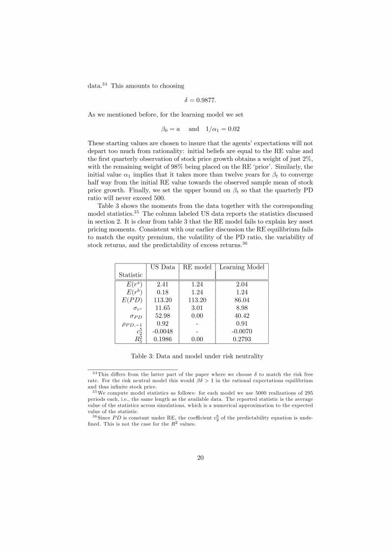
These starting values are chosen to insure that the agents’ expectations will notdepart too much from rationality: initial beliefs are equal to the RE value andthe first quarterly observation of stock price growth obtains a weight of just 2%,with the remaining weight of 98% being placed on the RE ‘prior’. Similarly, theinitial value α1 implies that it takes more than twelve years for βt to convergehalf way from the initial RE value towards the observed sample mean of stockprice growth. Finally, we set the upper bound on βt so that the quarterly PDratio will never exceed 500.Table 3 shows the moments from the data together with the corresponding

model statistics.35 The column labeled US data reports the statistics discussedin section 2. It is clear from table 3 that the RE model fails to explain key assetpricing moments. Consistent with our earlier discussion the RE equilibrium failsto match the equity premium, the volatility of the PD ratio, the variability ofstock returns, and the predictability of excess returns.36

US Data RE model Learning ModelStatistic

E(rs) 2.41 1.24 2.04E(rb) 0.18 1.24 1.24

E(PD) 113.20 113.20 86.04σrs 11.65 3.01 8.98σPD 52.98 0.00 40.42

ρPD,−1 0.92 - 0.91c52 -0.0048 - -0.0070R25 0.1986 0.00 0.2793

Table 3: Data and model under risk neutrality

34This differs from the latter part of the paper where we choose δ to match the risk freerate. For the risk neutral model this would βδ > 1 in the rational expectations equilibriumand thus infinite stock price.35We compute model statistics as follows: for each model we use 5000 realizations of 295

periods each, i.e., the same length as the available data. The reported statistic is the averagevalue of the statistics across simulations, which is a numerical approximation to the expectedvalue of the statistic.36 Since PD is constant under RE, the coefficient c52 of the predictability equation is unde-

fined. This is not the case for the R2 values.

20

In table 3, the learning model shows a considerably higher volatility of stockreturns, high volatility and high persistence of the PD ratio, and the coeffi-cients and R2 of the excess predictability regressions all move strongly in thedirection of the data. This is consistent with our earlier discussion about theprice dynamics implied by learning. Clearly, the statistics of the learning modeldo not match the moments in the data quantitatively, but the purpose of thetable is to show that allowing for small departures from rationality substantiallyimproves the outcome. This is surprising, given that the model adds only onefree parameter (1/α1) relative to the RE model; additional simulations we con-ducted show that the qualitative improvements provided by the model are veryrobust to changes in 1/α1, as long as it is neither too close to zero - in whichcase the model behaves as the RE model - nor too large - in which case themodel delivers too much volatility.

Table 3 also shows that the learning model delivers a positive equity pre-mium. To understand why this occurs it proves useful to re-express the stockreturn between period 0 and period T as the product of three terms

TYt=1

Pt +Dt

Pt−1=

TYt=1

Dt

Dt−1| {z }=R1

·µPDT + 1

PD0

¶| {z }

=R2

·T−1Yt=1

PDt + 1

PDt| {z }=R3

.

The first term (R1) is independent of the way expectations are formed, thuscannot contribute to explaining the emergence of an equity premium in thelearning model. The second term (R2) can potentially generate an equity pre-mium if the terminal price dividend ratio in the learning model (PDT ) is onaverage higher than under rational expectations.37 Yet, our simulations showthat the opposite is the case: under learning the terminal price dividend ratio islower (on average) than under rational expectations; this term thus generates anegative premium under learning. The equity premium must thus be due thebehavior of the last component (R3). This term gives rise to an equity premiumvia a mean effect and a volatility effect.The mean effect emerges if agents’ beliefs βt tend to converge ‘from below’

towards their rational expectations value. Less optimistic expectations aboutstock price growth during the convergence process imply lower stock prices andthereby higher dividend yields, i.e., higher ex-post stock returns. Our simula-tions show that the mean effect is indeed present and that on average the pricedividend ratio under learning is lower than under rational expectations. Thisexplanation for the equity premium resembles the one advocated by Cogley andSargent (2006).Besides this mean effect, there exists also a volatility effect, which emerges

from the convexity of R3 in the price dividend ratio. It implies that the ex-post equity premium is higher under learning since the price dividend ratio

37The value of PD0 is the same under learning and rational expectations since initial ex-pectations in the learning model are set equal to the rational expectations value.

21

has a higher variance than under rational expectations.38 The volatility effectsuggests that the inability to match the variability of the price dividend ratioand the equity premium are not independent facts and that models that gen-erate insufficient variability of the price dividend ratio also tend to generate aninsufficiently high equity premium.

4 Baseline model with risk aversionThe remaining part of the paper shows that the learning model can also quan-titatively account for the moments in the data, once one allows for moderatedegrees of risk-aversion, and that this finding is robust to a number of alter-native specifications. Here we present the baseline model with risk aversion,our simple baseline specification for the learning rule (OLS), and the baselinecalibration procedure. The quantitative results for this baseline specificationare discussed in section 5, while section 6 illustrates the robustness of our quan-titative findings to a variety of changes in the learning rule and the calibrationprocedure.

4.1 Learning under risk aversion

We now present the baseline learning model with risk aversion and show thatthe insights from the risk neutral model extend in a natural way to the casewith risk aversion.The investor’s first-order conditions (3) together the assumption that agents

know the conditional expectations of dividends deliver the asset pricing equationunder learning:39

Pt = δ eEt

µµDt

Dt+1

¶σPt+1

¶+ δEt

ÃDσt

Dσ−1t+1

!(23)

With rational expectations about future price, the equilibrium stock price is40

PREt =

δβRE

1− δβREDt (24)

βRE = a1−σe−σ(1−σ)s2

2 (25)

38The data suggest that this convexity effect is only moderately relevant: for the US data1927:2-2000:4, it is at most 0.16% in quarterly real terms, thus explains about 8% of the equitypremium.39As in section 2, we impose the market clearing condition Ct = Dt and will associate

consumption with dividends in the data. This is not entirely innocuous as dividend growthin the data is considerably more volatile than consumption growth, as discussed by Campbelland Cochrane (1999) in detail. Section 6 will illustrate the robustness of our quantitativefindings when allowing for the fact that Ct 6= Dt.40Assuming Et Dt

Dt+1

σPREt+1 = βREPRE

t in (3), one obtains (24). Using the latter to

substiute for prices in the assumed relationship above delivers (25).

22

implying

Et

µµDt

Dt+1

¶σPREt+1

¶= βREPRE

t .

In close analogy to the risk-neutral case, we consider learning agents whoseexpectations in (23) are of the form

eEt

µµDt

Dt+1

¶σPt+1

¶= βtPt (26)

where βt denotes agents’ best estimate of E (Dt/Dt+1)σPt+1/Pt, i.e., their ex-

pectations of risk-adjusted stock price growth. For βt = βRE agents have ratio-nal expectations and if βt → βRE beliefs will satisfy Asymptotic Rationality.As a baseline specification, we consider again the case where agents use OLS

to formulate their expectations of future (risk-adjusted) stock price growth

βt = βt−1 +1

αt

∙µDt−2Dt−1

¶σPt−1Pt−2

− βt−1

¸(27)

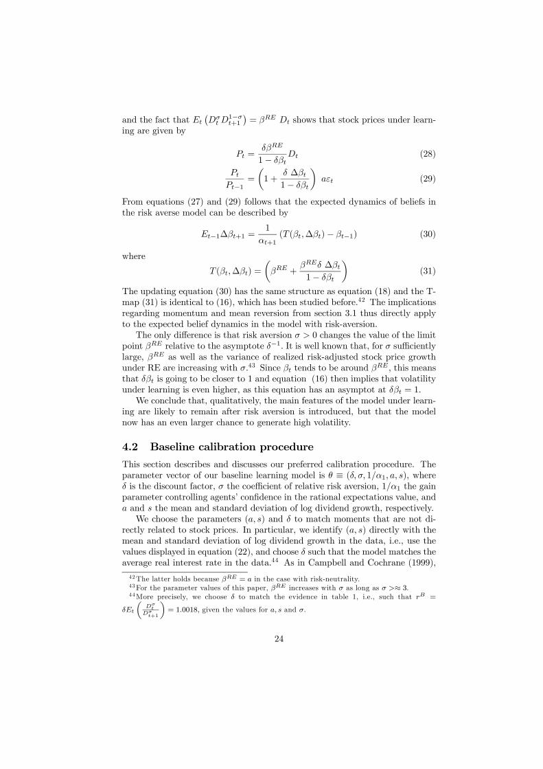
where the gain sequence 1/αt continues to be described by (20).In the spirit of allowing for only small deviations from rationality, we restrict

initial beliefs to be rational (β0 = βRE) and assume that agents have high butless than full confidence in this belief (1/α1 close to but not equal to zero).Appendix A.6 shows that learning will cause beliefs to globally converge to RE,i.e., βt → βRE and

¯PREt − Pt

¯→ 0 almost surely. The learning scheme thus

satisfies Asymptotic Rationality.For σ = 0 the setup above reduces to the risk-neutral model with learn-

ing studied in section 3. For σ > 0 the setup is isomorphic with that underrisk neutrality, except that 1. the beliefs β now have an interpretation as risk-adjusted stock price growth rather than simple stock price growth; 2. The term(Dt−2/Dt−1)

σ now enters the belief updating formula (27). Since for sufficientlylarge σ the variance of realized risk-adjusted stock price growth under RE in-creases with σ, the latter implies that larger risk aversion is likely to generatemore volatility in beliefs and, therefore, of actual prices under learning.41 Thiswill improve the ability of the learning model to match the moments in the data.As in the risk-neutral case we need to impose a projection facility to insure

that beliefs satisfy the inequality (12). To facilitate model calibration, describedin the next section, we impose a differentiable projection facility. The detailsare describe in appendix A.5.3. As before, the projection facility insures thatthe PD ratio will never exceed a value of 500.Finally, we show that beliefs continue to display momentum and mean-

reversion, similar to the case with risk-neutrality. Using equations (26), (23),

41The formula for the variance risk adjusted stock price growth under rational expectationsis

V ARDt−2Dt−1

σ PREt−1

PREt−2

= a2(1−σ)e(−σ)(1−σ)s2

2 (e(1−σ)2s2 − 1)

This variance reaches a minimum for σ = 1.

23

and the fact that Et

¡Dσt D

1−σt+1

¢= βRE Dt shows that stock prices under learn-

ing are given by

Pt =δβRE

1− δβtDt (28)

PtPt−1

=

µ1 +

δ ∆βt1− δβt

¶aεt (29)

From equations (27) and (29) follows that the expected dynamics of beliefs inthe risk averse model can be described by

Et−1∆βt+1 =1

αt+1(T (βt,∆βt)− βt−1) (30)

where

T (βt,∆βt) =

µβRE +

βREδ ∆βt1− δβt

¶(31)

The updating equation (30) has the same structure as equation (18) and the T-map (31) is identical to (16), which has been studied before.42 The implicationsregarding momentum and mean reversion from section 3.1 thus directly applyto the expected belief dynamics in the model with risk-aversion.The only difference is that risk aversion σ > 0 changes the value of the limit

point βRE relative to the asymptote δ−1. It is well known that, for σ sufficientlylarge, βRE as well as the variance of realized risk-adjusted stock price growthunder RE are increasing with σ.43 Since βt tends to be around βRE , this meansthat δβt is going to be closer to 1 and equation (16) then implies that volatilityunder learning is even higher, as this equation has an asymptot at δβt = 1.We conclude that, qualitatively, the main features of the model under learn-

ing are likely to remain after risk aversion is introduced, but that the modelnow has an even larger chance to generate high volatility.

4.2 Baseline calibration procedure

This section describes and discusses our preferred calibration procedure. Theparameter vector of our baseline learning model is θ ≡ (δ, σ, 1/α1, a, s), whereδ is the discount factor, σ the coefficient of relative risk aversion, 1/α1 the gainparameter controlling agents’ confidence in the rational expectations value, anda and s the mean and standard deviation of log dividend growth, respectively.We choose the parameters (a, s) and δ to match moments that are not di-

rectly related to stock prices. In particular, we identify (a, s) directly with themean and standard deviation of log dividend growth in the data, i.e., use thevalues displayed in equation (22), and choose δ such that the model matches theaverage real interest rate in the data.44 As in Campbell and Cochrane (1999),

42The latter holds because βRE = a in the case with risk-neutrality.43For the parameter values of this paper, βRE increases with σ as long as σ >≈ 3.44More precisely, we choose δ to match the evidence in table 1, i.e., such that rB =

δEtDσt

Dσt+1

= 1.0018, given the values for a, s and σ.

24

our model exhibits a constant real interest rate, and since agents are assumedto know the dividend process, the interest rate is the same as with rationalexpectations. The baseline learning model thus can not improve fit along thisdimension.This leaves us with two free parameters (σ, 1/α1) and seven remaining stock

price moments from table 1bS 0 ≡ ³ bE(rs), bE(PD), bσrs , bσPD, bρPDt,PDt−1 ,bc52, bR25, ,´As discussed in detail in section 2, these moments quantitatively capture thestock price facts we seek to explain.The parameters (σ, 1/α1) have no immediate link to any of the moments inbS, i.e., it is far from obvious which of the moments to choose for calibration.

In addition, some of these moments have a rather large standard deviationin the data (see table 4 below). Matching any of them exactly thus appearsarbitrary, as one obtains rather different parameters estimates depending onwhich moment is chosen for calibration. For these reasons, we depart from theusual calibration practice and choose the values for (σ,α1) so as to fit all sevenstatistics in the vector bS as good as possible.As measures of goodness-of-fit we focus on the t-ratiosbSi − Si(θc)bσSi (32)

where bSi denotes the i-th moment from the data, Si(θ) the corresponding mo-ment implied by the model, and bσSi the standard deviation of the moment. Wethen choose the parameterization (σ, 1/α1) that minimizes the sum of squaredt-ratios, where the sum is taken over for all seven moments. This implies thatmoments with a larger standard deviation receive less weight, i.e., are matchedless precisely, but also that the calibration result is invariant to a potential rescal-ing of the moments. The details of the procedure are defined and explained inappendix A.5.In the calibration literature it is standard to construct bσSi in equation (32)

by looking at the model implied standard deviation of the considered moment.It is also common to conclude that the model’s fit is satisfactory if the t-ratiosare less than, say, two or three in absolute value. In our application, thispractice has a number of problems. First, by choosing a model parameterizationthat gives rise to large standard deviations for the considered moment, i.e., aparameterization implying very unsharp predictions, one appears to improve‘fit’. For example, a model predicting implausibly large volatility of stock priceswill ‘fit’ very well, simply because the standard deviation of most moments willbe very high and the t-ratios (32) correspondingly low. Second, we wish toassess model performance across a variety of alternative model specifications.Using model implied standard deviations would then cause the goodness-of-fitcriterion to vary across models, an aspect we do not feel comfortable with.To avoid these problems we prefer to find an estimate of the standard de-

viation of each statistic bσSi that is based purely on data sources. We show in25

appendix A.5 how to obtain consistent estimates of these standard deviationsfrom the data. With these estimates we then follow the calibration literature,i.e., use these resulting t-ratios as our measure of ‘fit’ for each sample statisticand claim to have a good fit if this ratio is below two or three.The procedure just described may appear somewhat like estimation by the

method of simulated moments, and using the t-ratios as measures of fit mayappear like using test statistics. In appendix A.5 we describe how this interpre-tation could be made, but we do not wish to interpret our procedure as a formaleconometric method. The distribution of the parameters and test statisticsfor these formal estimation methods relies on asymptotics, but asymptoticallyour baseline learning model is indistinguishable from RE. Therefore, one wouldhave to rely on short-sample statistics, but short-sample econometric theory isunderdeveloped and developing it is a full research agenda in itself.Summing up, we interpret the method just described as a way to pick the

parameter (σ, α1) in a systematic way, such that the model has a good chanceto meet the data, but where the model could also be rejected. In this way weattempt to convince the reader that the learning model is able to quantitativelyaccount for key features of stock price data.

5 Quantitative resultsWe now evaluate the quantitative performance of the baseline learning modelwhen using the baseline calibration approach described in the previous section.Our results are summarized in table 4 below. The second and third column

of the table report the asset pricing moments from the data that we seek tomatch and the estimated standard deviation of the moments, respectively. Thetable shows that some of the reported moments, e.g., σPD, are estimated ratherimprecisely; our calibration procedure will automatically place less emphasis onmatching these moments.The calibrated parameters values of the learning model are reported at the

bottom of the table and appear reasonable on a priori grounds. The coeffi-cient of relative risk aversion is well within the ranges used in previous studies.Moreover, the gain parameter 1/α1 is close to zero, reflecting the tendency ofthe data to give large (but less than full) weight to the RE prior about stockprice growth. As has been explained before, high values of the gain 1/α1 tendto give rise to too much volatility because beliefs are then very volatile. Thecalibrated gain reported in the table implies that when updating beliefs in theinitial period, the RE prior receives a weight of approximately 98,4% and thefirst quarterly observation a weight of about 1.6%.

26

US Data OLSStatistics std t-ratio

E(rs) 2.41 0.45 2.39 0.05E(PD) 113.20 15.15 109.01 0.28

σrs 11.65 2.88 12.91 -0.44σPD 52.98 16.53 65.47 -0.76

ρPDt,PDt−1 0.92 0.02 0.94 -1.14c52 -0.0048 0.002 -0.0079 1.54R25 0.1986 0.083 0.2972 -1.19

Parameters: σ = 4.47 1/α1 = 0.0162

Table 4: Moments and parameters,baseline model and baseline calibration

The fourth column in table 4 reports the moments implied by the calibratedlearning model. The learning model performs remarkably well. In particular,the model with risk aversion maintains the high variability and serial correlationof the PD ratio and the variability of stock returns, as in section 3. In addition,it now succeeds in matching the mean of the PD ratio and also matches theequity premium.45 As discussed in section 2 before, it is natural that the excessreturn regressions can be explained reasonably well once the serial correlationof the PD is matched.Clearly, the point estimate of some model moments does not match exactly

the observed moment in the data, but this tends to occur for moments that, inthe short sample, have a large variance. This is shown in the last column oftable 4 which reports the goodness-of-fit measures (t-ratios) for each consideredmoment. The t-ratios are all well below two and thus well within what is a 95%confidence interval, if this were be a formal econometric test (which it is not).In summary, the results of table 4 show that introducing learning substan-

tially improves the fit of the model relative to the case with RE and is overallvery successful in quantitatively accounting for the empirical evidence describedin section 2. We find this result remarkable, given that we used the simplestversion of the asset pricing model and combined it with the simplest availablelearning mechanism.

6 RobustnessThis section shows that the quantitative performance of the model is robust tomany extensions. We start by exploring alternative models of learning, thenconsider alternative calibration procedures. In all cases, the model explains thestylized facts described in section 2.

45Recall that the discount factor has been chosen so as to match the sample mean of therisk-free real interest rate. Matching the mean stock return, therefore, implies that the modelalso matches the risk premium.

27

Learning about dividends. In the baseline model we assume agents knowthe conditional expectation of dividends. This is done to simplify the expo-sition and because learning about dividends has been considered in previouspapers.46 Since it may appear inconsistent to assume that agents know the div-idend growth process but do not know how to forecast stock prices, we considera model where agents learn about dividend growth and stock price growth. InAppendix A.4 we lay out the model and show that, while the analysis is moreinvolved, the basic results do not change. Table 5 below shows the quantitativeresults with learning about dividends using the baseline calibration proceduredescribed in section 5. It shows that introducing dividend learning does notlead to significant changes.

Constant gain learning. An undesirable feature of the OLS learningscheme is that volatility of asset prices decreases over time, which may seemcounterfactual. Therefore, we introduce a learning scheme with a constant gain,i.e., assume that the weight on the forecast error in the learning scheme isconstant: αt = α1 for all t.47 Beliefs then respond to forecast errors in the sameway throughout the sample and asset price volatility does not decrease. Asdiscussed extensively in the learning literature, such a learning scheme improvesforecasting performance when there are changes in the environment. Agentswho suspect the existence of switches in the average growth rate of prices orfundamentals, for example, may be reasonably expected to use such a scheme.Table 5 reports the quantitative results for the constant gain model using thebaseline calibration approach. For obvious reasons, stock prices are now morevolatile, even if the initial gain is substantially lower than in the baseline case.Overall, the fit of the model improves, especially regarding the evidence onexcess return predictability.48

Switching weights. We now introduce a learning model in which the gainswitches over time, as in Marcet and Nicolini (2003).49 The idea is to combineconstant gain with OLS, using the former in periods in which forecast errors arelarge and the latter when the forecast error is low. We report the quantitativeresults in Table 5, which are very similar to those with pure constant gainlearning. The latter occurred because the model was frequently in ‘constantgain mode’.

46E.g., Timmermann (1993, 1996).47The derivations for this model are as in section 4 and require only changing the evolution

of α.48We do not use constant gain as our main learning scheme because βt does then not

converge, i.e., we loose asymptotic rationality. Nevertheless, constant gain would generatebetter forecasts than OLS in a setup where there are trend switches in fundamentals. Sincethere is some evidence of such switches in the data, we believe that a model with constantgain will eventually generate better forecasts in a model with trend switches and fit the databetter. We leave this for future research.49The advantage of using switching gains, relative to using simple constant gain, is that

under certain conditions, the laerning model converges to RE, i.e., Asymptotic Rationality isindeed preserved.

28

US Data Learning about Div. Constant gain Switching weightsStatistic t-ratio t-ratio t-ratio

E(rs) 2.41 2.38 0.07 2.19 0.50 2.18 0.51E(PD) 113.20 105.04 0.54 117.94 -0.31 117.72 -0.30

σrs 11.65 12.31 -0.23 13.91 -0.78 13.62 -0.68σPD 52.98 59.38 -0.39 73.59 -1.25 73.04 -1.21

ρPDt,PDt−1 0.92 0.94 -1.26 0.93 -0.24 0.93 -0.20c52 -0.0048 -0.0087 1.9446 -0.0063 0.745 -0.0064 0.7767R25 0.1986 0.3276 -1.5580 0.2278 -0.352 0.2273 -0.3465

Parameters:σ 4.64 3.31 3.03

1/α1 0.0163 0.0069 0.0070Table 5: Robustness, Part I

Consumption data. Throughout the paper we made the simplifying as-sumption Ct = Dt and calibrated this process to dividend data, mainly becausein studying stock price volatility the data on dividends has to be brought out.In the data, consumption and dividend growth display rather different volatil-ities. Therefore, we now allow for Ct 6= Dt and calibrate the consumption anddividend process separately to the data.50 While dividends are as before, we set

Ct+1

Ct= aεct+1 for ln εct ∼ iiN(−s

2c

2; s2c)

The presence of two shocks modifies the equations for the RE version of themodel in a well known way and we do not describe it in detail here. We calibratethe model by following Campbell and Cochrane (1999) and set sc = s

7 andρ(εc, ε) = .2.51 We also have to slightly modify our calibration approach becausechoosing δ to match exactly the average interest rate will result in δβRE > 1 forreasonable values of σ, while we require δβRE < 1 to have a finite stock price.Therefore, we simply include the risk-free interest rate in our set of moments tobe matched, and δ joins σ and 1/α1 in the minimization of the sum of squaredt-ratios, which now includes also t-ratio for the interest rate.The quantitative results are reported in table 6 below, which shows that

we fit the data very well for the moments reported in the table. Yet, it turnsout that the value for δ implies E

¡rb¢= 0.83 in the model, while in the data

we have bE ¡rb¢ = 0.18 with a standard deviation of bσrb = 0.23. This resultsin a t-ratio equal to -2.86. Therefore, this particular model does not explainthe risk-free interest rate or, equivalently, does not explain the equity premium

50This would require changing the model described in section 4 to one with an exogenousendowment that is added to the budget constraint of the agent and to the resource constraint.The modification is obvious and we omit the details.51We take these ratios and values from table 1 in Campbell and Cochrane (1999), which is

based on a slightly shorter sample than the one used in this paper.

29

puzzle. Nevertheless, it appears that we are still close to explaining it: if thiswere a valid econometric test for the moment bE ¡rb¢ (which it is not), it wouldbe explained at the 99% confidence level. We do not wish to make much ofthis quasi-rejection, as we do not see the objective of this paper as matchingperfectly all moments. In particular, the equity premium is not the main focusof this paper and the literature suggests many reasonable extensions that wouldfurther improve the fit of the model in this dimension. Our conclusion fromthis robustness exercise is that it confirms the finding that the introduction oflearning improves considerably the ability to match the data on stock prices.

Full weighting matrix We now investigate the robustness of our findingsto changes in the calibration procedure. In an econometric MSM setup, onewould have to find the parameters that minimize a quadratic form with a fullinstead of a diagonal weighting matrix, see the discussion around equation (44)in appendix A.5. As table 6 shows, we still obtain a good model fit when usingsuch a full weighting matrix. The degree of relative risk aversion increases andthe ability to match the serial correlation of the PD ratio deteriorates. Weare not sure why this happens, but it may be related to the fact that the fullweighting matrix is nearly singular, a situation that causes the estimates tobe nearly ill-defined. We do not pursue this issue further, but simply wantedillustrate to a reader interested in econometrics: first, results do not changemuch if one uses more econometric-based calibration techniques; second, it isnot immediate how to formulate an econometric test of the model with standardMSM tools, see also the discussion in appendix A.5.

Model-generated standard deviations As a final exercise we demon-strate the robustness of our finding to using t-ratios based on model-generatedstandard deviations. We do this to show to readers who are partial to calibra-tion that results are largely unchanged if we use their preferred criterion of fit.As discussed before, we do not use this criterion in the remaining part of thepaper because the comparison across models is awkward, and because some ofthe robustness exercises (the exercise with a separate process for consumptiondata and the exercise with the full weighting matrix) could not be performedusing model-generated variances. The quantitative results reported in the lasttwo columns of table 6 show that the model performs very well when usingmodel-generated standard deviations and that calibrated parameter values re-main largely unchanged.

30

US Data Ct 6= Dt OLS, Full matrix bσSi from ModelStatistics t-ratio t-ratio t-ratio

E(rs) 2.41 2.01 0.90 2.14 0.60 2.33 0.30E(PD) 113.20 114.51 -0.09 105.35 0.52 109.64 0.12

σrs 11.65 10.43 0.43 12.84 -0.41 12.68 -0.27σPD 52.98 61.57 -0.52 63.70 -0.65 64.94 -0.61

ρPDt,PDt−1 0.92 0.95 -1.42 0.97 -2.40 0.95 -0.52c52 -0.0048 -0.0091 2.112 -0.0061 0.6373 -0.0077 1.045R25 0.1986 0.2422 -0.526 0.3442 -1.7584 0.3020 -.563

Parameters:σ 3.23 7.08 4.51

1/α1 0.0248 0.0089 0.0154Table 6: Robustness, Part II

The previous robustness exercises allowed for deviations from the baselinemodel and baseline calibration one step at a time. We also performed a varietyof other robustness tests that combine more than one of the features of therobustness test described above. We found that the model continues to explainthe moments well in all these cases.

7 Conclusions and OutlookA one parameter learning extension of the most standard asset pricing modelstrongly improves the ability of the model to quantitatively account for a numberof asset pricing facts. This outcome is remarkable, given the difficulties docu-mented in the empirical asset pricing literature in accounting for these facts. Thedifficulties of rational expectations models suggests that learning processes maybe more relevant for explaining empirical phenomena than previously thought.Indeed, it seems that the most convincing case for models of learning can bemade by explaining facts that appear ‘puzzling’ from the rational expectationsviewpoint. This is what this paper does.The simple setup presented in this paper could be extended in a number

of interesting ways and also applied to study other substantive questions. Oneavenue that we currently explore is to ask whether learning processes can ac-count also for the otherwise puzzling behavior of exchange rates. Clearly, theability of simple models of learning to explain puzzling empirical phenomena inmore than one market would further increase confidence in that learning-inducedsmall deviations from rationality are indeed economically relevant.

31

A Appendix

A.1 Data Sources

Our data is for the United States and has been downloaded from ‘The GlobalFinancial Database’ (http://www.globalfinancialdata.com). The period coveredis 1925:4-2005:4. For the subperiod 1925:4-1998:4 our dataset corresponds veryclosely to Campbell’s (2003) data (http://kuznets.fas.harvard.edu/~campbell/data.html).In the calibration part of the paper we use moments that are based on the

same number of observations. Since we seek to match the return predictabilityevidence at the five year horizon, the effective sample end for the means andstandard deviations reported in table 1 has been shortened by five years to2000:4. In addition, due to the seasonal adjustment procedure for dividendsdescribed below and the way we compute the standard errors for the momentsdescribed in appendix A.5, the effective starting date was 1927:2.To obtain real values, nominal variables have been deflated using the ‘USA

BLS Consumer Price Index’ (Global Fin code ‘CPUSAM’). The monthly priceseries has been transformed into a quarterly series by taking the index value ofthe last month of the considered quarter.The nominal stock price series is the ‘SP 500 Composite Price Index (w/GFD

extension)’ (Global Fin code ‘_SPXD’). The weekly (up to the end of 1927) anddaily series has been transformed into quarterly data by taking the index valueof the last week/day of the considered quarter. Moreover, the series has beennormalized to 100 in 1925:4.As nominal interest rate we use the ‘90 Days T-Bills Secondary Market’

(Global Fin code ‘ITUSA3SD’). The monthly (up to the end of 1933), weekly(1934-end of 1953), and daily series has been transformed into a quarterly se-ries using the interest rate corresponding to the last month/week/day of theconsidered quarter and is expressed in quarterly rates, i.e., not annualized.Nominal dividends have been computed as follows

Dt =

µID(t)/ID(t− 1)

IND(t)/IND(t− 1) − 1¶IND(t)

where IND denotes the ‘SP 500 Composite Price Index (w/GFD extension)’described above and ID is the ‘SP 500 Total Return Index (w/GFD extension)’(Global Fin code ‘_SPXTRD ’). We first computed monthly dividends andthen quarterly dividends by adding up the monthly series. Following Campbell(2003), dividends have been deseasonalized by taking averages of the actualdividend payments over the current and preceding three quarters.

A.2 Proof of mean reversion

To proof mean reversion of beliefs we need two additional technical assumptions:1. We slightly strengthen (12) to 0 < βt < βU < δ−1; 2. Letting

Dt ≡ inf∆

∂ft∂∆

(∆)

32

we assumeP

tDt = ∞, which is standard in the stochastic control literature.It is satisfied by all the learning mechanisms considered in this paper and isneeded to avoid beliefs getting stuck away from the fundamental value simplybecause updating ceases too quickly.We start proving mean reversion for the case βt > a+ η. Fix η and choose

ε = η¡1− δβU

¢. Since ε > 0 it cannot be that ∆βt0 ≥ ε for all t0 > t as this

would imply βt → ∞, violating the upper bound on β. Therefore, for somet0 > t we have ∆βt0 < ε.Take t0 > t to be the first period where ∆βt0 < ε. At this point βt0 ≥ βt and

thereforeβt0 > a+ η

and

T (βt0 ,∆βt0) = a+∆βt0

1− δβt0< a+

ε

1− δβU= a+ η

where the inequality uses ∆βt0 < ε and that βU is an upper bound for β; theequality on the right follows from the way ε is chosen above. The previous tworelations imply

βt0 > T (βt0 ,∆βt0)

which together with (18) and the fact that ft is increasing and ft(0) = 0 gives

∆βt0+1 = ft0+1 (T (βt0 ,∆βt0)− βt0) < 0 (33)

There are two possibilities: either

i) βt0+j ≤ a+ η eventually for some j > 0, or

ii) βt0+j > a+ η for all j > 0.

In case i) we are done. We now prove that case ii) is impossible by setting upan inductive argument that leads to a contradiction. For any j > 0, ∆β

t0+j < 0

implies a +∆βt0+j1−δβt0+j

< a and if ii) holds T (βt0+j ,∆βt0+j) < βt0+j . From theproperties of ft it follows ∆βt0+j+1 < 0. Thus, ∆βt0+j < 0 implies ∆βt0+j+1 < 0for any j > 0 with the initial condition given by (33). The negativity of ∆β

t0+jfor j > 0 implies the first inequality below

a+∆βt0+j1− δβt0+j

− βt0+j < a− βt0+j < a− (a+ η) = −η for all j > 0 (34)

with the second following from ii). We thus have

∆βt0+j+1 = ft0+j+1

µa+

∆βt0+j1− δβt0+j

− βt0+j

¶< ft0+j+1 (−η) ≤ −ηDt0+j+1

where the first inequality follows from (34) and the second from the mean valuetheorem and Dt ≥ 0. The previous result implies

βt0+j =

jXi=1

∆βt0+i + βt0 ≤ −ηjX

i=1

Dt0+i

33

for all j > 0. The assumptionP

tDt = ∞ would then imply βt → −∞ whichviolates our assumptions that ft is such that βt > 0 at all times.For the case βt < a − η we choose ε = η and we can use a symmetric

argument to make the proof.

A.3 Details on the phase diagram

The second order difference equation (18) describing the deterministic evolutionof beliefs allows to construct non-linear first-order learning dynamics in the(βt, βt−1) plane. For clarity, we define x0t ≡ (x1,t, x2,t) ≡ (βt, βt−1) , whosedynamics are given by

xt+1 =

Ãx1,t + ft+1

³a+

aδ(x1,t−x2,t)1−δx1,t − x1,t

´x1,t

!The zeros of the phase diagram are ∆x2 = 0 at points x1 = x2 and ∆x1 = 0 forx2 =

1δ −

x1(1−δx1)aδ . So the zeroes for ∆x1 and ∆x2 intersect are at x1 = x2 = a

which is the REE and, interestingly, at x1 = x2 = δ−1 which is the limit ofthe rational bubble equilibrium. Moreover, as is easy to verify ∆x2 > 0 forx1 > x2 and ∆x1 > 0 for x2 < 1

δ −x1(1−δx1)

aδ . These results give rise to thephase diagram shown in figure 2.

A.4 Model with learning about dividends

This section considers agents who learn to forecast future dividends in additionto forecast future price. We make the arguments directly for the general modelwith risk aversion from section 4. Equation (23) then becomes

Pt = δ eEt

µµCt

Ct+1

¶σPt+1

¶+ δ eEt

ÃDσt

Dσ−1t+1

!Under RE one has

Et

ÃDσt

Dσ−1t+1

!= Et

ÃD1−σt+1

D−σt

!= Et

õDt+1

Dt

¶1−σ!Dt

= Et

³(aε)

1−σ´Dt

= βREDt

This justifies that learning agents will forecast future dividends according to

eEt

ÃD1−σt+1

D−σt

!= γtDt

where γt is agents’s best estimate of eEt

µ³Dt+1

Dt

´1−σ¶, which can be interpreted

as risk-adjusted dividend-growth. In close analogy to the learning setup for

34

future price we assume that agents’ estimate evolves according to

γt = γt−1 +1

αt

õDt−1Dt−2

¶1−σ− γt−1

!(35)

which can be given a proper Bayesian interpretation. In the spirit of allowingfor only small deviations from rationality, we assume that the initial belief iscorrect

γ0 = βRE .

Moreover, the gain sequence αt is the same as the one used for updating theestimate for βt. Learning about βt remains to be described by equation (27).With these assumptions realized price and price growth are given by

Pt =δγt

1− δβtDt

PtPt−1

=γtγt−1

µ1 +

δ4βt1− δβt

¶aεt

The map T from perceived to actual expectations of the risk-adjusted price

growth Pt+1Pt

³Dt

Dt+1

´σin this more general model is given by

T (βt+1,∆βt+1) ≡γt+1γt

µβRE +

βREδ ∆βt+11− δβt+1

¶(36)

which differs from (31) only by the factor γt+1γt. From (35) it is clear that γt+1

γt

evolves exogenously and that limt→∞γt+1γt

= 1 since limt→∞ γt = βRE andαt → ∞. Thus, for medium to high values of αt and initial beliefs not too farfrom the RE value, the T-maps with and without learning about dividends arevery similar.For the deterministic setting with risk-neutrality considered in section 3, one

has γt = γ0 = a and βRE = a so that (36) becomes identical to (16).

A.5 Calibration procedure

This section describes the details of our calibration approach and explains howwe estimate the standard deviation of the sample statistics reported in table 4.

Let N be the sample size, (y1, ...yN ) the observed data sample, with ytcontaining m variables. We consider the sample statistics S(MN) which are afunction of the sample momentMN with S : Rq → Rs being a statistic functionthat maps moments into the considered statistics. The statistic function isrequired because some of the statistics we seek to match, see table 4, are notmoments but functions of moments.52 Let h : Rm → Rq denote the function52This is the case, for example, for the correlation and the R2 coefficients. The standard

case of matching moments is obtained when S is the identity.

35

determining the sample moments on which our statistics are based, i.e., MN ≡1N

PNt=1 h(yt). The explicit expressions for h(·) and S(·) for our particular

application are stated in Appendix A.5.1 below.

Given the sample statistics, we now explain how we compute the correspond-ing model statistics for a given model parameterization θ ∈ Rn. Let ωs denotea realization of shocks and (y1(θ, ωs), ...yN (θ, ωs)) the random variables corre-sponding to a history of length N generated by the model for shock realizationωs. Furthermore, let

MN (θ, ωs) ≡ 1

N

NXt=1

h(yt(θ, ωs))

denote the model moment for realization ωS and

S(MN (θ, ωs))

the corresponding model statistic. The model statistics we wish to report arethe expected value of the statistic across possible shock realizations:

S(MN (θ)) = E [S(MN (θ, ωs))]

One can obtain a numerical approximation to the theoretical model statisticS(MN (θ)) by averaging (for a given a parameter vector θ) across a large num-ber of simulations of length N the statistics S(MN (θ, ω

s)) implied by eachsimulation. We report this average in the tables of the main text.

Now that we have explained how to compute statistics in the data and themodel, we explain how we calibrate the parameters so as to match the modelstatistics to the statistics of the data. Let Si(MN ) denote the i-th statisticfrom the data, Si(MN (θ) the corresponding statistic from the model, and bσSian estimate for the standard deviation of the i-th statistic. How we obtain bσSiwill be explained in detail below. The baseline parameter choice bθN is thenfound as follows

bθN ≡ argminθ

7Xi=1

µSi(MN )− Si(MN (θ))bσSi

¶2(37)

subject to the restrictions on a, s, δ that have been described in the text. Ourprocedure thus tries to match the model statistics as closely as possible tothe data statistics, but gives less weight to statistics with a larger standarddeviation. Notice that the calibration result is invariant to a rescaling of thevariables of interest and that with the available two parameters (α1, σ), it isgenerally not possible to match all seven moments numerically, unless the modelis closely related to the data.To be able to use standard numerical procedures to solve the minimization

problem (37), we slightly modify the projection facility described in (21) to

36

insure that it is continuously differentiable. Appendix A.5.3 describes this indetail.

We now explain how we obtain the estimate for the standard deviation ofthe i-th statistic bσSi . We start by discussing desirable asymptotic properties ofsuch an estimate and then explain how it has been constructed.We would like to have an estimator bσSi that converges to the standard

deviation of the statistic sufficiently fast, so that asymptotically the t-ratio hasa standard normal distribution, i.e., we require

√NSi(MN )− Si(MN (θ0))bσ2Si → N (0, 1) in distribution (38)

asN →∞ and where θ0 denotes the true value of the parameters and Si(MN (θ0))the corresponding true value of the i-th model statistic. Once we have such anestimator, it is possible to interpret t-ratios as goodness of fit measures thatcould be given an asymptotic interpretation.We now explain how to find an estimate for the full covariance matrix bΣS,N

of model statistics from a sample of N observations such that

bΣS,N → ΣS almost surely, for (39)√N [S(MN )− S(MN (θ0))]→ N (0,ΣS) (40)

as N →∞. Note that the bσ2Si in (37) and (38) are simply the diagonal entriesof bΣS,N . Let M0 = E [h(yt(θ0, ω

s))] denote the theoretical moment at the trueparameter value. Assume y to be stationary and ergodic, S to be continuouslydifferentiable at M0, and

Sw ≡∞X

j=−∞E£(h(yt)−M0) (h(yt−j)−M0)

0¤<∞ (41)

We then have ΣS in (39) given by

ΣS =∂S(M0)

∂M 0 Sw∂S 0(M0)

∂M(42)

This follows from standard arguments: by the mean value theorem

√N [S(M0)− S(MN )] =

∂S(fMN )

∂M 0

√N [M0 −MN ] (43)

where fMN is some convex combination of MN and M0.53 Under stationarityand ergodicity of y, we have MN →M0 a.s. by the ergodic theorem. Since fMN

53As is well known, a different MN is needed for each row of S but this is inconsequentialfor the proof and we ignore it here.

37

is between MN and M0, this implies fMN → M0 a.s. and, since∂S(·)∂M 0 has been

assumed continuous at M0 we have that

∂S(fMN )

∂M 0 → ∂S(M0)

∂M 0 a.s.

From the central limit theorem√N (M0 −MN )→ N(0, Sw) in distribution

Plugging the previous two relationships into (43) shows (42).Therefore, by taking an estimate Sw,N that converges a.s. to Sw and by

taking bΣS,N ≡ ∂S(MN )

∂M 0 Sw,N∂S 0(MN)

∂M

one obtains property (38). Explicit expression for ∂S(MN )/∂M0 are given in

appendix A.5.2. It now only remains to find the estimates Sw,N from the data.We follow standard practice and employ the Newey West estimator, which trun-cates the infinite sum in (41) and weighs the autocovariances in a particular way.This is standard and we do not describe the details here.

Our baseline procedure for choosing parameter values described above canbe thought of as a hybrid between the method of simulated moments (MSM)and calibration.We differ from fully-fledged MSM (described below) because we do not per-

form any formal estimation, we do not attempt to use an optimal weightingmatrix, and we do not adjust for the degrees of freedom in the asymptotic dis-tribution of the goodness of fit tests, and because we do not think of this asan exercise in accepting or rejecting the model. Instead,our procedure is sim-ply a way of systematically choosing parameter values that allows us to displaythe behavior of the model and to interpret the t-ratios as giving a measure ofcloseness.We also differ from calibration because we do not pin down each parameter

with a given moment and use the remaining moments to test the model. Instead,we let the algorithm find the parameters (σ, α1) that best fit the seven consideredmoments of the data. Moreover, in our procedure the standard deviation of themoment bσSi is computed from the data. This is useful for a number of reasons.First, the standard practice in calibration of using model-determined standarddeviations gives an incentive to the researcher to generate models with highstandard deviations, i.e., unsharp predictions, as these appear to improve fit.Second, if bσSi is determined from the data, it is constant across alternativemodels allows for model comparisons in a meaningful way.

In addition to the baseline calibration procedure above, we engage in a ro-bustness exercise, reported under the heading ‘full matrix’ in table 6, which iscloser to MSM. In particular, we choose parameters to solvebθN ≡ argmin

θ[S(MN (θ))− S(MN )]

0 bΣ−1S,N [S(MN (θ))− S(MN )] (44)

38

This way of fitting the model is less intuitive but generally has the advantagethat bΣ−1S,N is an optimal weighting matrix so the estimate should be closer to

the true model parameter. One problem we encountered is that bΣS,N is nearlysingular and it is well known that in this case the weighting matrix in shortsamples does not produce good results. While the literature suggests ways toaddress this problem, this is clearly beyond the scope of this paper.

A.5.1 The statistic and moment functions

This section gives explicit expressions for the statistic function S(·) and themoment functions h(·) introduced in appendix A.5. The 7 statistics we considercan be expressed as function of eight sample moments MN,i (i = 1, . . . , 8):54

S(MN ) ≡

⎡⎢⎢⎢⎢⎢⎢⎢⎢⎣

E(rst )E(PDt)σrstσPDt

ρPDt,PDt−1

c52R25

⎤⎥⎥⎥⎥⎥⎥⎥⎥⎦=

⎡⎢⎢⎢⎢⎢⎢⎢⎢⎢⎢⎢⎣

MN,1

MN,2qMN,3 − (MN,1)

2qM4 − (MN,2)

2

MN,5−(MN,2)2

MN,4−(MN,2)2

c52(MN )R25(MN )

⎤⎥⎥⎥⎥⎥⎥⎥⎥⎥⎥⎥⎦where the functions c52(M) and R25(M) defining the OLS and R2 coefficients ofthe excess returns regressions, respectively, are

c5(MN ) ≡∙

1 MN,2

MN,2 MN,4

¸−1 ∙MN,6

MN,8

¸R25(MN ) ≡ 1−

MN,7 − [MN,6,MN,8] c5(MN )

MN,7 − (MN,6)2

The underlying sample moments are

MN ≡

⎡⎢⎢⎢⎢⎣M1,N

.

.

.M8,N

⎤⎥⎥⎥⎥⎦ ≡ 1

N

NXt=1

h(yt)

54As in the main text, we slightly abuse notation and let, for example, E rS denote thesample mean of stock returns.

39

where h(·) and yt are defined as

h(yt) ≡

⎡⎢⎢⎢⎢⎢⎢⎢⎢⎢⎢⎢⎢⎣

rstPDt

(rst )2

(PDt)2

PDt PDt−1rs,20t−20³rs,20t−20

´2rs,20t−20PDt−20

⎤⎥⎥⎥⎥⎥⎥⎥⎥⎥⎥⎥⎥⎦, yt ≡

⎡⎢⎢⎢⎢⎢⎢⎢⎢⎢⎢⎢⎣

PDt

Dt/Dt−1PDt−1

Dt−1/Dt−2...

PDt−19Dt−19/Dt−20

PDt−20

⎤⎥⎥⎥⎥⎥⎥⎥⎥⎥⎥⎥⎦where rs,20t denotes the stock return over 20 quarters, which can be computedusing from yt using (PDt,Dt/Dt−1, ..., PDt−19,Dt−19/Dt−20).

A.5.2 Derivatives of the statistic function

This appendix gives explicit expressions for ∂S(·)/∂M 0 using the statistic andmoment functions stated in appendix A.5.1. Straightforward but tedious algebrashows

∂Si∂Mi

= 1 for i = 1, 2

∂Si∂Mi

=1

2Si(M)for i = 3, 4

∂Si∂Mj

=−Mj

Si(M)for (i, j) = (3, 1), (4, 2)

∂S5∂M2

=2M2(M5 −M4)

(M4 −M22 )2

,∂S5∂M5

=1

M4 −M22

,∂S5∂M4

= − M5 −M22

(M4 −M22 )2

∂S6∂Mj

=∂c52(M)

∂Mjfor i = 2, 4, 6, 8

∂S7∂Mj

=[M6,M8]

∂c5(M)∂Mj

M7 −M26

for j = 2, 4

∂S7∂M6

=

hc51(M) + [M6,M8]

∂c5(M)∂M6

i ¡M7 −M2

6

¢− 2M6 [M6,M8] c

5(M)

(M7 −M26 )2

∂S7∂M7

=M26 − [M6,M8] c

5(M)

(M7 −M26 )2

∂S7∂M8

=c52(M) + [M6,M8]

∂c5(M)∂M8

M7 −M26

Using the formula for the inverse of a 2x2 matrix

c5(M) =1

M4 −M22

∙M4M6 −M2M8

M8 −M2M6

¸

40

we have

∂c5(M)

∂M2=

1

M4 −M22

µ2M2c

5(M)−∙M8

M6

¸¶∂c5(M)

∂M4=

1

M4 −M22

µ−c5(M) +

∙M6

0

¸¶∂c5(M)

∂M6≡ 1

M4 −M22

∙M4

−M2

¸∂c5(M)

∂M8≡ 1

M4 −M22

∙−M2

1

¸All remaining terms ∂Si/∂Mj not listed above are equal to zero.

A.5.3 Differentiable projection facility

As discussed in the main text, we need to introduce a feature that preventsperceived stock price growth from being higher than δ−1, so as to insure a finiteasset price. In addition, it is convenient for our calibration exercises if thelearning scheme is a continuous and differentiable function, see the discussionin appendix A.5. We thus modify the simple discontinuous projection facilitydescribed in (21) by one that ‘phases in’ more gradually. We define

β∗t = βt−1 +1

αt

"µDt−1Dt−2

¶−σPt−1Pt−2

− βt−1

#(45)

and modify the updating scheme (27) to

βt =

½β∗t if β∗t ≤ βL

w(β∗t )βU + [1− w(β∗t )]β

L otherwise(46)

where βU is the upper bound on beliefs, chosen to insure that the impliedPD ratio is always less than a certain upper bound UPD, βL < βU is somearbitrary level of beliefs above which the projection facility starts to operate,and w(·) : R+ → [0, 1] is a weighting function. We choose the weighting functionto guarantee that the updating scheme is continuously differentiable w.r.t. β∗tand that limβ∗t→∞ βt = βU . In particular, we define

w(β∗t ) =

∙1− βU − βL

β∗t + βU − 2βL

¸.

With this weighting function

limβ∗t→(βL)−

βt = limβ∗t→(βL)+

βt = βL

limβ∗t→(βL)−

∂βt∂β∗t

= limβ∗t→(βL)+

∂βt∂β∗t

= 1

41

In our numerical applications we choose βU so that the implied PD ratio neverexceeds UPD = 500 and βL = δ−1 − 2(δ−1 − βU ), which implies that thedampening effect of the projection facility starts to come into effect for valuesof the PD ratio above 250.In table 7 below we show that the modification of the projection facility

to a continuous function does not significantly affect our quantitative results.Using the baseline model calibration from table 4, we report in table 7 themodel moments if instead of the continuous projection facility one uses theprojection facility (21) with UPD = 500. The main difference to the baselineresults consists of an increase in the volatility of the PD ratio (σPD). Clearly,this emerges because the continuous projection facility dampens beliefs alreadybefore they reach the upper bound implied by UPD. Obviously, by choosingalternative values of σ and 1/α1 one can obtain moments for the model witha non-continuous projection facility that are even closer to the moments in thedata.

Non-continuous projection facilityStatistics t-ratio

E(rs) 2.09 0.72E(PD) 119.51 -0.42

σrs 12.96 -0.45σPD 81.09 -1.70

ρPDt,PDt−1 0.94 -1.20c52 -0.0064 0.81R25 0.2981 -1.20

Parameters: σ = 4.47 1/α1 = 0.0162

Table 7: Robustness to projection facility

A.6 Convergence of least squares to RE

We show convergence directly for the general learning model with risk aversionfrom section 4. To obtain convergence we need bounded shocks. In particular,we assume existence of some Uε <∞ such that

Prob(εt < Uε) = 1

Prob(ε1−σt < Uε) = 1

Furthermore, we assume that the projection facility is not binding in the REequilibrium

PREt

Dt=

δβRE

1− δβRE< UPD

where βRE = Eh(aεt)

1−σiand PRE

t is the price in the RE equilibrium.

42

We first show that the projection facility will almost surely cease to bebinding after some finite time. In a second step, we prove that βt converges toβRE from that time onwards.The projection facility implies

βt =

⎧⎨⎩ βt−1 + α−1t

³(aεt−1)

−σ Pt−1Pt−2

− βt−1´

if δa

1−δ βt−1+α−1t (aεt−1)

−σ Pt−1Pt−2

−βt−1< UPD

βt−1 otherwise(47)

If the lower equality applies one has (aεt−1)−σ Pt−1

Pt−2≥ βt−1 and this gives rise

to the following inequalities

βt ≤ βt−1 + α−1t

µ(aεt−1)

−σ Pt−1Pt−2

− βt−1

¶(48)

|βt − βt−1| ≤ α−1t

¯µ(aεt−1)

−σ Pt−1Pt−2

− βt−1

¶¯(49)

which hold for all t. Substituting recursively in (48) for past β’s delivers

βt ≤1

t− 1 + α1

⎛⎝t−1Xj=0

(aεj)−σ Pj

Pj−1+ (α1 − 1) β0

⎞⎠=

t

t− 1 + α1

⎛⎝1t

t−1Xj=0

(a εj)1−σ

+α1 − 1

tβ0

⎞⎠| {z }

=T1

+1

t− 1 + α1

⎛⎝t−1Xj=0

δ ∆βj1− δβj

(aεj)1−σ

⎞⎠| {z }

=T2

(50)

where the second line follows from (29). Since T1 → βRE for t→∞ a.s., βt willeventually be bounded away from its upper bound if we can establish |T2|→ 0a.s.. This is achieved by noting that

|T2| ≤1

t− 1 + α1

t−1Xj=0

δ (a εj)1−σ

1− δβj|∆βj |

≤ Uε

t− 1 + α1

t−1Xj=0

a1−σδ |∆βj |1− δβj

≤ Uε

t− 1 + α1

a1−σUPD

βRE

t−1Xj=0

|∆βj | (51)

where the first inequality results from the triangle inequality and the fact thatboth εj and 1

1−δβj are positive, the second inequality follows from the a.s. boundon εj , and the third inequality from the bound on the price dividend ratioinsuring that δβRE (1− δβj)

−1 < UPD. Next, observe that

(aεj)−σ Pt

Pt−1=1− δβt−11− δβt

(aεt)1−σ

<(aεt)

1−σ

1− δβt<

a1−σUεUPD

δβRE(52)

43

where the equality follows from (28), the first inequality from βt−1 > 0, and thesecond inequality from the bounds on ε and PD. Using result (52), equation(49) implies

|βt − βt−1| ≤ α−1t

¯(aεt)

−σ Pt−1Pt−2

− βt−1

¯≤ α−1t

µa1−σUεUPD

δβRE+ δ−1

¶where the second inequality follows from the triangle inequality and the factthat βt−1 < δ−1. Since αt →∞ this establishes that |∆βt|→ 0 and, therefore,

1t−1+α1

Pt−1j=0 |∆βj | → 0. Then (51) implies that |T2| → 0 a.s. as t → ∞. By

taking the lim sup on both sides on (50), it follows from T1 → βRE and |T2|→ 0that

lim supt→∞

βt ≤ βRE

a.s.. The projection facility is thus operative infinitely often with probabilityzero. Therefore, there exists a set of realizations ω with measure one and at < ∞ (which depends on the realization ω) such that the projection facilitydoes not operate for t > t.

We now proceed with the second step of the proof. Consider, for a givenrealization ω, a t for which the projection facility is not operative after thisperiod. Then the upper equality in (47) holds for all t > t and simple algebragives

βt =1

t− t+ αt

⎛⎝t−1Xj=t

(aεj)−σ Pj

Pj−1+ αt βt

⎞⎠=

t− t

t− t+ αt

⎛⎝ 1

t− t

t−1Xj=t

(aεj)1−σ

+1

t− t

t−1Xj=t

δ ∆βj1− δβj

(aεj)1−σ

+αtt− t

βt

⎞⎠(53)

for t > t. Equations (48) and (49) now hold with equality for t > t. Similaroperations as before then deliver

1

t− t

t−1Xj=t

δ ∆βj1− δβj

(aεj)1−σ → 0

a.s. for t→∞. Finally, taking the limit on both sides of (53) establishes

βt → βRE

a.s. as t→∞.¥

44

ReferencesAbel, A. B. (1990): “Asset Prices under Habit Formation and Catching Upwith the Joneses,” American Economic Review, 80, 38—42.

Adam, K. (2003): “Learning and Equilibrium Selection in a Monetary Over-lapping Generations Model with Sticky Prices,” Review of Economic Studies,70, 887—908.

(2007): “Experimental Evidence on the Persistence of Output andInflation,” Economic Journal, 117, 603—636.

Allen, F., S. Morris, and H. S. Shin (2006): “Beauty Contest and IteratedExpectations in Asset Markets,” Review of Financial Studies, 19, 719—752.

Branch, W., and G. W. Evans (2006): “Asset Return Dynamics and Learn-ing,” University of Oregon mimeo.

Bray, M. M., and D. M. Kreps (1987): “Rational Learning and RationalExpectations,” in Arrow and the Ascent of Modern Economic Theory, ed. byG. Feiwel, pp. 597—625. New York University Press, New York.

Brennan, M. J., and Y. Xia (2001): “Stock Price Volatility and EquityPremium,” Journal of Monetary Economics, 47, 249—283.

Brock, W. A., and C. H. Hommes (1998): “Heterogeneous Beliefs andRoutes to Chaos in a Simple Asset Pricing Model,” Journal of EconomicDynamics and Control, 22, 1235—1274.

Bullard, J., and J. Duffy (2001): “Learning and Excess Volatility,” Macro-economic Dynamics, 5, 272—302.

Campbell, J. Y. (2003): “Consumption-Based Asset Pricing,” in Handbook ofEconomics and Finance, ed. by G. M. Constantinides, M. Harris, and R. Stulz,pp. 803—887. Elsevier, Amsterdam.

Campbell, J. Y., and J. H. Cochrane (1999): “By Force of Habit:A Consumption-Based Explanation of Aggregate Stock Market Behavior,”Journal of Political Economy, 107, 205—251.

Carceles-Poveda, E., and C. Giannitsarou (2006): “Asset Pricing withAdaptive Learning,” SUNY Stoney Brook and Cambridge University mimeo.

Cecchetti, S., P.-S. Lam, and N. C. Mark (2000): “Asset Pricing withDistorted Beliefs: Are Equity Returns Too Good to Be True?,” AmericanEconomic Review, 90, 787—805.

Cogley, T., and T. J. Sargent (2006): “The Market Price of Risk and theEquity Premium: A Legacy of the Great Depression?,” New York Universitymimeo.

45

LeRoy, S. F., and R. Porter (1981): “The Present-Value Relation: TestBased on Implied Variance Bounds,” Econometrica, 49, 555—574.

Mankiw, G., D. Romer, and M. D. Shapiro (1985): “An Unbiased Reex-amination of Stock Market Volatility,” Journal of Finance, 40(3), 677—687.

Marcet, A., and J. P. Nicolini (2003): “Recurrent Hyperinflations andLearning,” American Economic Review, 93, 1476—1498.

Marcet, A., and T. J. Sargent (1989): “Convergence of Least SquaresLearning Mechanisms in Self Referential Linear Stochastic Models,” Journalof Economic Theory, 48, 337—368.

Shiller, R. J. (1981): “Do Stock Prices Move Too Much to Be Justified bySubsequent Changes in Dividends?,” American Economic Review, 71, 421—436.

(2005): Irrational Exuberance: Second Edition. Princeton UniversityPress, Princeton, USA.

Timmermann, A. (1993): “How Learning in Financial Markets Generates Ex-cess Volatility and Predictability in Stock Prices,” Quarterly Journal of Eco-nomics, 108, 1135—1145.

(1996): “Excess Volatility and Predictability of Stock Prices in Au-toregressive Dividend Models with Learning,” Review of Economic Studies,63, 523—557.

46