stock market volatility and learning philippe weil for a very interesting discussion. davide...

WORK ING PAPER SER IE SNO 862 / FEBRUARY 2008

STOCK MARKETVOLATILITYAND LEARNING

by Klaus Adam, Albert Marcetand Juan Pablo Nicolini

WORKING PAPER SER IE SNO 862 / FEBRUARY 2008

In 2008 all ECBpublications

feature a motiftaken from the10 banknote.

STOCK MARKET VOLATILITY ANDLEARNING1

Klaus Adam2,Albert Marcet 3

and Juan Pablo Nicolini 4

This paper can be downloaded without charge fromhttp : //www.ecb.europa.eu or from the Social Science Research Network

electronic library at ht tp : //ssrn.com/abstract_id=1090276.

1 Thanks go to Luca Dedola, Katharina Greulich, Jaume Ventura and Joachim Voth for interesting comments and suggestions. We particularlythank Philippe Weil for a very interesting discussion. Davide Debortoli has supported us with outstanding research assistance and manysuggestions. Marcet acknowledges support from CIRIT (Generalitat de Catalunya), DGES (Ministry of Education and Science), CREI, theBarcelona Economics program of XREA and the Wim Duisenberg fellowship from the European Central Bank. The views expressed

herein are solely those of the authors and do not necessarily reflect the views of the European Central Bank.2 European Central Bank and CEPR, Postal address: European Central Bank, Kaiserstrasse 29, 60311 Frankfurt am Main, Germany;

e-mail: [email protected] Institut d’Anàlisi Economica CSIC, Universitat Autònoma de Barcelona, 08193 Bellaterra, Spain;

e-mail: [email protected] Universidad Torcuato di Tella, Miñones 2177, Capital Federal, (C1428ATG) Argentina;

e-mail: [email protected]

© European Central Bank, 2008

AddressKaiserstrasse 2960311 Frankfurt am Main, Germany

Postal addressPostfach 16 03 1960066 Frankfurt am Main, Germany

Telephone+49 69 1344 0

Websitehttp://www.ecb.europa.eu

Fax+49 69 1344 6000

All rights reserved.

Any reproduction, publication andreprint in the form of a differentpublication, whether printed orproduced electronically, in whole or inpart, is permitted only with the explicitwritten authorisation of the ECB or theauthor(s).

The views expressed in this paper do notnecessarily reflect those of the EuropeanCentral Bank.

The statement of purpose for the ECBWorking Paper Series is availablefrom the ECB website, http://www.ecb.europa.eu/pub/scientific/wps/date/html/index.en.html

ISSN 1561-0810 (print)ISSN 1725-2806 (online)

3ECB

Working Paper Series No 862February 2008

Abstract 4

Non-technical summary 5

1 Introduction 6

2 Facts 9

3 The risk neutral case 143.1 Analytical results 163.2 The Risk Neutral Model with OLS 20

4 Baseline model with risk aversion 264.1 Learning under risk aversion 264.2 Baseline calibration procedure 28

5 Quantitative results 30

6 Robustness 32

7 Conlusions and Outlook 36

Appendix 36

References 50

European Central Bank Working Paper Series 51

CONTENTS

4ECBWorking Paper Series No 862February 2008

Abstract

Introducing bounded rationality into a standard consumption basedasset pricing model with a representative agent and time separable pref-erences strongly improves empirical performance. Learning causes mo-mentum and mean reversion of returns and thereby excess volatility, per-sistence of price-dividend ratios, long-horizon return predictability and arisk premium, as in the habit model of Campbell and Cochrane (1999),but for lower risk aversion. This is obtained, even though we restrict con-sideration to learning schemes that imply only small deviations from fullrationality. The �ndings are robust to the particular learning rule usedand the value chosen for the single free parameter introduced by learn-ing, provided agents forecast future stock prices using past informationon prices.

JEL Class. No.: G12, D84

Keywords: asset pricing, learning, near-rational price forecasts

5ECB


This paper presents and estimates a very simple stock price model and showsthat this model is able to replicate a number of important asset pricing facts.This �nding is remarkable because it has proven surprisingly di¢cult to repli-cate these facts within the realm of rational expectations models. Speci�cally,rational expectations models with standard (time-separable) preference assump-tions are largely unable to explain: why the price dividend ratio of stocks is sovolatile and displays such persistent swings; why stock returns are so much morevolatile than dividend growth; why high (low) price dividend ratios predict low(high) future stock returns over the medium to long term (next 1-10 years); orwhy real stock returns are so much higher than the real returns on short-termbonds.The empirical success of the learning model in replicating all these facts

is due to a slight relaxation of the rational expectations assumption. Moreprecisely, the model assumes that investors� expectations about future capitalgains are revised slightly upwards (downwards) if they observe higher (lower)than previously expected capital gains in the stock market. We show how evenweak feedback of this kind can give rise to persistent and large swings in stockprices and thereby replicate the empirically observed stock price behavior.The postulated feedback from observed capital gains to expected future cap-

ital gains can be very weak because this feedback mechanism is largely self-reinforcing. In particular, if investors� capital gain expectations have increased,this justi�es paying a higher price for stocks. Therefore, just because investorshave become more optimistic, there will be tendency for prices to increase ata rate that is larger than the fundamentally justi�ed growth rate. This rein-forces the initial belief of higher capital gains and imparts �momentum� on stockprices, producing large and sustained deviations of the price dividend ratio fromits sample mean. Since the momentum e¤ect operates also in the opposite di-rection, i.e., for downward revisions in expected capital gains, the postulatedfeedback produces large and mean reverting swings in the price dividend ratio.As we explain in the paper in the detail, the presence of these swings allows themodel to replicate all the asset pricing facts mentioned above.To impose discipline on the modeling of deviations from fully rational expec-

tations, we introduce a learning scheme that will cause agents to asymptoticallylearn the truth, i.e., to make rational forecasts eventually. This learning schemeintroduces a single free parameter, which can take on values between zero andone, and allows to gauge how much expectations deviate from rational expec-tations during the transition phase. If this parameters is set equal to zero, oneshuts down completely the feedback from observed capital gains to expected fu-ture capital gains, causing the model to collapse to a rational expectations modelright away (which then cannot reproduce the empirical stock price behavior). Ifthis parameter is set equal to one, the feedback strength is maximal with agents�expectations about future capital gains then being given by the sample averageof historically observed capital gains. We show that values very close to zero(around 0.01 and 0.02), i.e., close to the rational expectations model, allow toreplicate the empirically observed stock price behavior.

Non-technical summary


"Investors, their con�dence and expectations buoyed by past price increases,bid up speculative prices further, thereby enticing more investors to do thesame, so that the cycle repeats again and again, .. "

Irrational Exuberance, Shiller (2005, p.56)

1 Introduction

The purpose of this paper is to show that a very simple asset pricing model is ableto reproduce a variety of stylized facts if one allows for small departures fromrational expectations. This result is somehow remarkable, since the literaturein empirical �nance had great di¢culties in developing dynamic equilibriumrational expectations models accounting for all the facts we consider.Our model is based on the representative agent time-separable utility endow-

ment economy developed by Lucas (1978). It is well known that the implicationsof this model under rational expectations are at odds with basic asset pricingobservations: in the data the price dividend ratio is too volatile and persistent,stock returns are too volatile and are negatively related to the price dividendratio in the long run, and the risk premium is too high. Our learning modelintroduces just one additional free parameter into Lucas� framework and quan-titatively accounts for all these observations. Since the learning model reducesto the rational expectations model if the additional parameter is set to zero andsince this parameter is close to zero throughout the paper, we consider the learn-ing model to represent only a small departure from rationality. Nevertheless,the behavior of equilibrium prices di¤ers considerably from the one obtainedunder rational expectations, implying that the asset pricing implications of thestandard model are not robust to small departures from rationality. As we doc-ument, this non-robustness is empirically encouraging, i.e., the model matchesthe data much better if this small departure from rationality is allowed for.A very large body of literature has documented that stock prices exhibit

movements that are very hard to reproduce within the realm of rational expec-tations and Lucas� tree model has been extended in a variety of directions toimprove its empirical performance. After many papers and a couple of decadesthis line of research has succeeded: Campbell and Cochrane (1999) are able toreproduce all the facts, albeit at the cost of imposing sophisticated non-time-separabilities in preferences and high e¤ective degrees of risk aversion. Ourmodel retains simplicity and moderate curvature in utility, but instead deviatesfrom rational expectations.The behavioral �nance literature tried to understand the decision making

process of individual investors by means of surveys, experiments and microevidence, exploring the intersection between economics and psychology. Oneof the main themes of this literature was to test the rationality hypothesis in

7ECB


asset markets, see Shiller (2005) for a non-technical summary. We borrow someof the economic intuition from this literature, but follow a di¤erent modelingapproach: we aim for a model that is as close as possible to the original Lucastree model, with agents who are quasi-rational and formulate forecasts usingstatistical models that imply only small departures from rational expectations.In the baseline learning model, we assume agents form their expectations re-

garding future stock prices with the most standard learning scheme used in theliterature: ordinary least squares (OLS).1 This rule has the property that in thelong run the equilibrium converges to rational expectations, but in the modelthis process takes a very long time, and the dynamics generated by learningalong the transition cause prices to be very di¤erent from the rational expecta-tions (RE) prices. This di¤erence occurs for the following reasons: if expecta-tions about stock price growth have increased, the actual growth rate of priceshas a tendency to increase beyond the fundamental growth rate, thereby rein-forcing the initial belief of higher stock price growth. Learning thus imparts�momentum� on stock prices and beliefs and produces large and sustained devi-ations of the price dividend ratio from its mean, as can be observed in the data.The model thus displays something like the �naturally occurring Ponzi schemes�described in Shiller�s opening quote above.As we mentioned, OLS is the most standard assumption to model the evolu-

tion of expectations functions in the learning literature and its limiting proper-ties have been used extensively as a stability criterion to justify or discard REequilibria. Yet, models of learning are still not commonly used to explain dataor for policy analysis.2 It is still the standard view in the economics researchliterature that models of learning introduce too many degrees of freedom, sothat it is easy to �nd a learning scheme that matches whatever observation onedesires. One can deal with this important methodological issue in two ways:�rst, by using a learning scheme with as few free parameters as possible, andsecond, by imposing restrictions on the parameters of the learning scheme toonly allow for small departures of rationality.3 These considerations promptedus to use an o¤-the-shelf learning scheme (OLS) that has only one free parame-ter. In addition, in the model at hand, OLS is the best estimator in the longrun, and to make the departure form rationality during the transition small, weassume that initial beliefs are at the rational expectations equilibrium, and thatagents initially have a very strong - but less than complete - con�dence in theseinitial beliefs.Models of learning have been used before to explain some aspects of asset

price behavior. Timmermann (1993, 1996), Brennan and Xia (2001) and Cogleyand Sargent (2006) consider Bayesian learning to explain various aspects of stock

1We show that results are robust to using other standard learning rules.2We will mention some exceptions along the paper.3Marcet and Nicolini (2003) dealt with this issue by imposing bounds on the size of the

mistakes agents can make in equilibrium. These bounds imposed discipline both on the typeof learning rule and on the exact value of the parameters in the learning rule. For the presentmodel we show that results are very robust to both the learning rule and the exact value ofthe single learning parameter.


prices. These authors assume that agents learn about the dividend process anduse the Bayesian posterior on the parameters of this process to estimate theexpected discounted sum of dividends. Therefore, while the beliefs of agentsin�uence the market outcomes, agents� beliefs remain una¤ected by marketoutcomes because agents learn only about an exogenous dividend process. Inthe language of stochastic control, these models are not self-referential. In thelanguage of Shiller, these models can not give rise to �naturally occurring Ponzischemes�. In contrast, we largely abstract from learning about the dividendprocess and consider learning on the future stock price using past observationsof price, so that beliefs and prices are mutually determined. It is preciselythe learning about future stock price growth and its self-referential nature thatimparts the momentum to expectations and, therefore, is key in explaining thedata.4

Other related papers by Bullard and Du¤y (2001) and Brock and Hommes(1998) show that learning dynamics can converge to complicated attractors, ifthe RE equilibrium is unstable under learning dynamics.5 Branch and Evans(2006) study a model where agents� expectations switch depending on whichof the available forecast models is performing best. By comparison, we look atlearning about the stock price growth rate, we address more closely the data,and we do so in a model where the rational expectations equilibrium is stableunder learning dynamics, so the departure from RE behavior occurs only alonga transition related to the sample size of the observed data. Also related isCárceles-Poveda and Giannitsarou (2006) who assume that agents know themean stock price and learn only about the deviations from the mean; they �ndthat the presence of learning does then not signi�cantly alter the behavior ofasset prices.6

The paper is organized as follows. Section 2 presents the stylized facts we fo-cus on and the basic features of the underlying asset pricing model, showing thatthis model cannot explain the facts under the rational expectations hypothesis.In section 3 we take the simplest risk neutral model and assume instead thatagents learn to forecast the growth rate of prices. We show that such a modelcan qualitatively deliver all the considered asset pricing facts and that learningconverges to rational expectations. We also explain how the deviations fromrational expectations can be made arbitrarily small. In Section 4 we presentthe baseline learning model with risk aversion and the baseline calibration pro-cedure. We also explain why we choose to calibrate the model parameters ina slightly di¤erent way than in standard calibration exercises. Section 5 showsthat the baseline model can quantitatively reproduce all the facts discussed insection 2. The robustness of our �ndings to various assumptions about the

4Timmerman (1996) analyzes in one setting also a self-referential model, but one in whichagents use dividends to predict future price. He �nds that this form of self-referntial learningdelivers lower volatility than settings with learning about the dividend process. It is thuscrucial for our results that agents use information on past price behavior to predict futureprice.

5 Stability under learning dynamics is de�ned in Marcet and Sargent (1989).6Cecchetti, Lam, and Mark (2000) determine the misspeci�cation in beliefs about future

consumption growth required to match the equity premium and other moments of asset prices.

9ECB


model, the learning rule, or the calibration procedure is illustrated in section 6.Readers interested in obtaining a glimpse of the quantitative performance

of the baseline learning model may - after reading section 2 - directly jump totable 4 in section 5.

2 Facts

This section describes stylized facts of U.S. stock price data and explains why itproved di¢cult to reproduce them using standard rational expectations models.The facts presented in this section have been extensively documented in theliterature. We reproduce them here as a point of reference for our quantitativeexercise in the latter part of the paper and using a single and updated data set.7

It is useful to start looking at the data through the lens of a simple dynamicstochastic endowment economy. Let Dt be the dividend of an inelastically sup-plied stock in period t, evolving according to

DtDt�1

= a"t (1)

where log "t � N( s2

2 ; s2) is i:i:d: and a � 1.8 Obviously, this assumption

guarantees E�

Dt

Dt�1

�= a and ��D

D= s.

Let the preferences of a representative consumer-investor be given by

E0

1X

t=0

�t U (Ct)

where Ct is consumption at time t, � the discount factor and U (�) strictlyincreasing and concave. We assume also there is a riskless real bond that paysone unit of consumption next period with certainty. With St denoting the end-of-period t stock holdings and Bt the bond holdings, the budget constraint is

Ct + Pbt Bt + Pt St = (Pt +Dt)St�1 +Bt�1;

where Pt is the real price of the stock and P bt the bond price. Under rationalexpectations, the equilibrium stock price must satisfy the consumer�s �rst ordercondition evaluated at Ct = Dt

Pt = �Et

�U�(Dt+1)

U�(Dt)(Pt+1 +Dt+1)

�(2)

which de�nes a mapping from the exogenous dividend process to the stochasticprocess of prices.9 The nature of this mapping obviously depends on the way

7Details on the underlying data sources are provided in Appendix A.1.8As documented in Mankiw, Romer and Shapiro (1985) and Campbell (2003), this is a

reasonable �rst approximation to the empirical behavior of quarterly dividends in the U.S. Itis also the standard assumption in the literature.

9 In the data, consumption is much less volatile than dividends. This raises importantissues that will be discussed later in the paper.


the intertemporal marginal rate of substitution moves with consumption. Forinstance, in the standard case of power preferences U(Ct) = C

��t and equation

(2) becomes

Pt = �Et

��DtDt+1

��(Pt+1 +Dt+1)

�(3)

With rational expectations about future price, the non-bubble equilibrium stockprice satis�es10

Pt =��RE

1� ��REDt (4)

where

�RE = a1��e��(1��)s2

2 (5)

Et

��DtDt+1

��PREt+1

�= �REPREt (6)

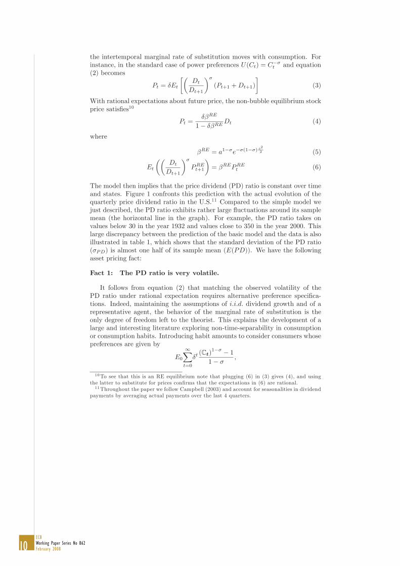
The model then implies that the price dividend (PD) ratio is constant over timeand states. Figure 1 confronts this prediction with the actual evolution of thequarterly price dividend ratio in the U.S.11 Compared to the simple model wejust described, the PD ratio exhibits rather large �uctuations around its samplemean (the horizontal line in the graph). For example, the PD ratio takes onvalues below 30 in the year 1932 and values close to 350 in the year 2000. Thislarge discrepancy between the prediction of the basic model and the data is alsoillustrated in table 1, which shows that the standard deviation of the PD ratio(�PD) is almost one half of its sample mean (E(PD)). We have the followingasset pricing fact:

Fact 1: The PD ratio is very volatile.

It follows from equation (2) that matching the observed volatility of thePD ratio under rational expectation requires alternative preference speci�ca-tions. Indeed, maintaining the assumptions of i:i:d: dividend growth and of arepresentative agent, the behavior of the marginal rate of substitution is theonly degree of freedom left to the theorist. This explains the development of alarge and interesting literature exploring non-time-separability in consumptionor consumption habits. Introducing habit amounts to consider consumers whosepreferences are given by

E0

1X

t=0

�t(Ct)1�� 11� � ;

10To see that this is an RE equilibrium note that plugging (6) in (3) gives (4), and usingthe latter to substitute for prices con�rms that the expectations in (6) are rational.11Throughout the paper we follow Campbell (2003) and account for seasonalities in dividend

payments by averaging actual payments over the last 4 quarters.

11ECB


Figure 1: Quarterly U.S. price dividend ratio 1927:1-2005:4

where Ct = H(Ct; Ct�1; Ct�2; :::) is a function of current and past consump-tion.12 A simple habit model has been studied by Abel (1990) who assumes

Ct =CtC�t�1

with � 2 (0; 1).13 In this case, the stock price under rational expectations is

PtDt

= A (a"t)�(��1) (7)

for some constant A, which shows that this model can give rise to a volatilePD ratio. Yet, with "t being i:i:d: the PD ratio will display no autocorrelation,which is in stark contrast to the empirical evidence. As �gure 1 illustrates, thePD ratio displays rather persistent deviations from its sample mean. Indeed, astable 1 shows, the quarterly autocorrelation of the PD ratio (denoted �PDt;�1)is very high. Therefore, this is the second fact we focus on:

Fact 2: The PD ratio is persistent.

The previous observations suggest that matching the volatility and persis-tence of the PD ratio under rational expectations would require preferences thatgive rise to a volatile and persistent marginal rate of substitution. This is the

12We keep power utility for expositional purposes only.13 Importantly, the main purpose of Abel�s model was to generate an �equity premium� - a

fact we discuss below - not to reproduce the behavior of the price dividend ratio.


avenue pursued in Campbell and Cochrane (1999) who engineer preferences thatcan match the behavior of the PD ratio we observe in Figure 1. Their speci-�cation also helps in replicating the asset pricing facts mentioned later in thissection, as well as other facts not mentioned here.14 Their solution requires,however, imposing a very high degree of relative risk aversion and relies on arather complicated structure for the habit function H (�).15In our model we maintain the assumption of standard time-separable con-

sumption preferences with moderate degrees of risk aversion. Instead, we relaxthe rational expectations assumption by replacing the mathematical expectationin equation (2) by the most standard learning algorithm used in the literature.Persistence and volatility of the price dividend ratio will then be the result ofadjustments in beliefs that are induced by the learning process.Before getting into the details of our model, we want to mention three addi-

tional asset pricing facts about stock returns. These facts have received consid-erable attention in the literature and are qualitatively related to the behaviorof the PD ratio, as we discuss below.

Fact 3: Stock returns are �excessively� volatile.

Starting with the work of Shiller (1981) and LeRoy and Porter (1981) it hasbeen recognized that stock prices are more volatile in the data than in standardmodels. Related to this is the observation that the volatility of stock returns(�rs) in the data is much higher than the volatility of dividend growth (��D=D),see table 1.16 The observed return volatility has been called �excessive� mainlybecause the rational expectations model with time separable preferences predictsapproximately identical volatilities. To see this, let rst denote the stock return

rst =Pt +Dt Pt�1

Pt�1=

"PtDt+ 1

Pt�1Dt�1

#DtDt�1

1 (8)

and note that with time-separable preferences and i:i:d: dividend growth, thePD ratio is constant and the term in the square brackets above is approximatelyequal to one.From equation (8) follows that excessive return volatility is qualitatively re-

lated to Fact 1 discussed above, as return volatility depends partly on the volatil-ity of the PD ratio.17 Yet, quantitatively return volatility also depends on thevolatility of dividend growth and - up to a linear approximation - on the �rsttwo moments of the cross-correlogram between the PD ratio and the rate of

14They also match the pro-cyclical variation of stock prices and the counter-cyclical variationof stock market volatility. We have not explored conditional moments in our learning model,see also the discussion at the end of this section.15The coe¢cient of relative risk aversion is 35 in steady state and higher still in states with

�low surplus consumption ratios�.16This is not due to accounting for seasonalities in dividends by taking averages: stock

returns are also about three times as volatile as dividend growth at yearly frequency.17Cochrane (2005) provides a detailed derivation of the qualitative relationship between

facts 3 and 1 for i:i:d: dividend growth.

13ECB


growth of dividends. Since the main contribution of the paper is to show theability of the learning model to account for the quantitative properties of thedata, we treat the volatility of returns as a separate asset pricing fact.

U.S. asset pricing facts, 1927:2-2000:4(quarterly real values, growth rates & returns in percentage terms)

Fact 1 Volatility of E(PD) 113.20PD ratio �PD 52.98

Fact 2 Persistence of �PDt;�1 0.92PD ratio

Fact 3 Excessive return �rs 11.65volatility ��D

D2.98

Fact 4 Excess return c52 -0.0048predictability R25 0.1986

Fact 5 Equity premium E [rs] 2.41E�rb�

0.18

Table 1: Stylized asset pricing facts

Fact 4: Excess stock returns are predictable over the long-run.

While stock returns are di¢cult to predict in general, the PD ratio is nega-tively related to future excess stock returns in the long run. This is illustratedin Table 2, which shows the results of regressing future cumulated excess re-turns over di¤erent horizons on today�s price dividend ratio.18 The absolutevalue of the parameter estimate and the R2 both increase with the horizon.As argued in Cochrane (2005, chapter 20), the presence of return predictabil-ity and the increase in the R2 with the prediction horizon are qualitatively ajoint consequence of Fact 2 and i:i:d: dividend growth. Nevertheless, we keepexcess return predictability as an independent result, since we are again inter-ested in the quantitative model implications. Yet, Cochrane also shows thatthe absolute value of the regression parameter increases approximately linearlywith the prediction horizon, which is a quantitative result. For this reason, we

18More precisely, the table reports results from OLS estimation of

Xt;t+s = cs1 + c

s2PDt + u

st

for s = 1; 3; 5; 10; where Xt;t+s is the observed real excess return of stocks over bonds betweent and t+ s. The second column of Table 2 reports estimates of cs2:


summarize the return predictability evidence using the regression outcome for asingle prediction horizon. We choose to include the 5 year horizon in table 1.19

Years Coe¢cient on PD, cs1 R2

1 -0.0008 0.04383 -0.0023 0.11965 -0.0048 0.198610 -0.0219 0.3285

Table 2: Excess stock return predictability

Fact 5: The equity premium puzzle.

Finally, and even though the emphasis of our paper is on moments of thePD ratio and stock returns, it is interesting to note that learning also improvesthe ability of the standard model to match the equity premium puzzle, i.e., theobservation that stock returns - averaged over long time spans and measured inreal terms - tend to be high relative to short-term real bond returns. The equitypremium puzzle is illustrated in table 1, which shows the average quarterly realreturn on bonds (E

�rbt�) being much lower than the corresponding return on

stocks (E (rst )).Unlike Campbell and Cochrane (1999) we do not include in our list of facts

any correlation between stock market data and real variables like consumptionor investment. In this sense, we follow more closely the literature in �nance. Inour model, it is the learning scheme that delivers the movement in stock prices,even in a model with risk neutrality in which the marginal rate of substitutionis constant. This contrasts with the habit literature where the movement ofstock prices is obtained by modeling the way the observed stochastic processfor consumption generates movements in the marginal rate of substitution. Thelatter explains why the habit literature focuses on the relationship between par-ticularly low values of consumption and low stock prices. Since this mechanismdoes not play a signi�cant role in our model, we abstract from these asset pricingfacts.

3 The risk neutral case

In this section we analyze the simplest asset pricing model assuming risk neu-trality and time separable preferences (� = 0 and Ct = Ct). The goal of thissection is to derive qualitative results and to show how the introduction of learn-ing improves the performance compared to a setting with rational expectations.Sections 4 and 5 present a formal quantitative model evaluation, extending theanalysis to risk-averse investors. With risk neutrality and rational expectations

19We also used longer and shorter horizons. This did not a¤ect our �ndings.

15ECB


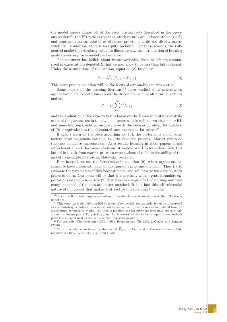
the model misses almost all of the asset pricing facts described in the previ-ous section:20 the PD ratio is constant, stock returns are unforecastable (i:i:d:)and approximately as volatile as dividend growth, i.e., do not display excessvolatility. In addition, there is no equity premium. For these reasons, the risk-neutral model is particularly suited to illustrate how the introduction of learningqualitatively improves model performance.The consumer has beliefs about future variables, these beliefs are summa-

rized in expectations denoted eE that we now allow to be less than fully rational.Under the assumptions of this section, equation (3) becomes21

Pt = � eEt (Pt+1 +Dt+1) (9)

This asset pricing equation will be the focus of our analysis in this section.Some papers in the learning literature22 have studied stock prices when

agents formulate expectations about the discounted sum of all future dividendsand set

Pt = eEt1X

j=1

�jDt+j (10)

and the evaluation of the expectation is based on the Bayesian posterior distrib-ution of the parameters in the dividend process. It is well known that under REand some limiting condition on price growth the one-period ahead formulationof (9) is equivalent to the discounted sum expression for prices.23

If agents learn on the price according to (10), the posterior is about para-meters of an exogenous variable, i.e., the dividend process. Market prices dothen not in�uence expectations. As a result, learning in these papers is notself-referential and Bayesian beliefs are straightforward to formulate. Yet, thislack of feedback from market prices to expectations also limits the ability of themodel to generate interesting �data-like� behavior.Here instead, we use the formulation in equation (9), where agents are as-

sumed to have a forecast model of next period�s price and dividend. They try toestimate the parameters of this forecast model and will have to use data on stockprices to do so. Our point will be that it is precisely when agents formulate ex-pectations on prices to satisfy (9) that there is a large e¤ect of learning and thatmany moments of the data are better matched. It is in fact this self-referentialnature of our model that makes it attractive in explaining the data.

20 Since the RE model implies a constant PD ratio the serial correlation of the PD ratio isunde�ned.21This equation is similarly implied by many other models, for example, it can be interpreted

as a no-arbitrage condition in a model with risk-neutral investors or can be derived from anoverlapping generations model. All that is required is that investors formulate expectationsabout the future payo¤ Pt+1 + Dt+1 and for investors� choice to be in equilibrium, today�sprice has to equal next period�s discounted expected payo¤.22For example, Timmermann (1993, 1996), Brennan and Xia (2001), Cogley and Sargent

(2006).23More precisely, equivalence is obtained if eEt [�] = Et [�] and if the no-rational-bubble

requirement limj!1 �j EPt+j = 0 must hold.


Focus on equation (9) not only improves empirical performance but can alsobe justi�ed formally. Note that the in�nite sum expression (10) requires dis-counting future dividends at the market discount rate. In a complete marketsetting, the market discount factor is identical to that of each investor at alltimes. This implies that an investor can obtain the in�nite sum (10) by simplyiterating on her �rst order condition (9). Under complete markets, equation(10) is thus a direct consequence of assuming that agents know their individ-ual decision problem.24 In more realistic settings, however, knowledge of theindividual decision problem ceases to imply (9). Suppose, for example, thatmarkets are incomplete, say, due to the presence of uninsurable liquidity shocksthat occassionally force investors to sell their stock. These shocks will drive awedge between individual and market discount factors, implying that individualinvestors cannot iterate on their Euler equations to obtain a correct formulationof how the market discounts future dividends. Instead, the investor will have toformulate beliefs about the future price to be able to value the asset.25 In ap-pendix A.2 we make this argument formally within an overlapping generations(OLG) model where agents are forced to sell their assets in the last period oftheir life. The RE equilibrium in the OLG economy is the same as in the Lucaseconomy, but young agents� relevant �rst order condition is given by (9). Sincethe same Euler equation does not apply when old, young agents cannot obtainthe in�nite sum (10) in a straightforward way.More informally, using the discounted sum (10) may also not be a very

robust way to price the asset, even if markets are complete. The discountedsum formulation implies that small approximation errors to the dividend processmay translate into a large pricing error. Speci�cally, if the forecast model fordividends is slightly misspeci�ed it is suboptimal to simply iterate on it to derivelong-horizon forecasts, i.e., the �law of iterated expectations� which is requiredto obtain the discounted sum may not hold.26 Learning about stock price isthen likely to be a more robust formulation of expectations. All this suggeststhat our one-period formulation is an interesting avenue to explore.

3.1 Analytical results

In this section we show that the introduction of learning changes qualitativelythe behavior of stock prices in the direction of improving the match of thestylized facts described above. At this point we consider a wide class of learningschemes that includes the standard rules used in the literature. This serves toprove that the e¤ects we discuss occur in a very general class of learning models.Later on we will restrict attention to learning schemes that forecast well withinthe model.24One also needs to assume that limj!1 �j eEPt+j = 0 holds25This may explain why participants in actual stock markets appear to care so much about

the selling price of the stock.26Adam (2007) provides experimental evidence of the breakdown of the law of iterated

expectations in an experiment where agents become gradually aware that they use a possiblymisspeci�ed forecasting model.

17ECB


We �rst trivially rewrite the expectation of the agent by splitting the sumin the expectation:

Pt = � eEt (Pt+1) + � eEt (Dt+1) (11)

We assume that agents know how to formulate the conditional expectation of thedividend eEt (Dt+1) = aDt, which amounts to assuming that agents have rationalexpectations about the dividend process. This simpli�es the discussion andhighlights the fact that it is learning about future prices that allows the modelto better match the data. Appendix A.5 shows that the pricing implications arevery similar if agents also learn how to forecast dividends.27

Agents are assumed to use a learning scheme in order to form a forecasteEt(Pt+1) based on past information. Equation (4) shows that under rationalexpectations Et [Pt+1] = aPt. As we restrict our analysis to learning rules thatbehave close enough to rational expectations, we specify expectations underlearning as

eEt [Pt+1] = �t Pt (12)

where �t > 0 denotes agents� time t estimate of gross stock price growth. For�t = a, agents� beliefs coincide with rational expectations. Also, if agents� beliefsconverge over time to the RE equilibrium (limt!1 �t = a), investors will realizein the long-run that they were correct in using the functional form (12). Yet,during the transition beliefs may deviate from rational ones.It remains to specify how agents update their beliefs �t. We consider the

following general learning mechanism

��t = ft

�Pt 1Pt 2

� �t 1�

(13)

for some exogenously chosen functions ft : R! R with the property

ft(0) = 0

f 0t > 0

We thus assume beliefs to adjust in the direction of the last prediction error,i.e., agents revise beliefs upwards (downwards), if they underpredicted (over-predicted) stock price growth in the past.28 Arguably, a learning scheme thatviolates these conditions would appear quite unnatural. For technical reasons,we also need to assume that the functions ft are such that

0 < �t < � 1 (14)

at all times. This rules out beliefs �t > � 1 which would imply that expectedstock returns exceed the inverse of the discount factor, prompting the represen-tative agent to have an in�nite demand for stocks at any stock price.27 In section 6 we verify this also quantitatively in a model with learning about dividends

and prices.28Note that �t is determined from observations up to period t � 1 only. The assumption

that the current price does not enter in the formulation of the expectations is common in thelearning literature and is entertained for simplicity. Di¢culties emerging with simultaneousinformation sets are discussed in Adam (2003).


Deriving quantitative and convergence results on learning will require spec-ifying the learning scheme more explicitly. At this point, we show that the keyfeatures of the model emerge within this more general speci�cation.

3.1.1 Stock prices under learning

Given the perceptions �t, the expectation function (12), and the assumption onperceived dividends, equation (11) implies that prices under learning satisfy

Pt =�aDt1� ��t

: (15)

Since �t and "t are independent, the previous equation implies that

V ar

�ln

PtPt�1

�= V ar

�ln1� ��t�11� ��t

�+ V ar

�ln

DtDt�1

�; (16)

and shows that price growth under learning is more volatile than dividendgrowth. Clearly, this occurs because the volatility of beliefs adds to the volatilitygenerated by fundamentals. While this intuition is present in previous models oflearning, e.g., Timmermann (1993), it will be particular to our case that under

more speci�c learning schemes V ar�ln 1��t

1��t+1

�is very high and remains high

for a long time.Equation (15) shows that the PD ratio is monotonically related to beliefs �t.

One can thus understand the qualitative dynamics of the PD ratio by studyingthe belief dynamics. To derive these dynamics notice

PtPt�1

= T (�t;��t) "t (17)

where

T (�;��) � a+ a� ��

1� �� (18)

It follows directly from (17) that T (�t;��t) is the actual expected stock pricegrowth given that the perceived price growth has been given by �t;��t. Substi-tuting (17) in the law of motion for beliefs (13) and using also (15) shows thatthe dynamics of �t (t � 1) are described by a second order stochastic di¤erenceequation

��t+1 = ft+1 (T (�t;��t)"t � �t) (19)

for given initial conditions (D0; P�1), and the initial belief �0. This equationcan not be solved analytically due to non-linearities,29 but it is still possible togain qualitative insights into the belief dynamics of the model. We do this inthe next section.29Notice that even in the case we consider below where ft is linear, the di¤erence equation

is non-linear due to the presence of T .

19ECB


3.1.2 Deterministic dynamics

To discuss the dynamics of beliefs �t under learning, we simplify matters byconsidering the deterministic case in which "t � 1. Equation (19) then simpli�esto

��t+1 = ft+1 (T (�t;��t) �t) : (20)

We thus restrict attention to the endogenous stock price dynamics generatedby the learning mechanism rather than the dynamics induced by exogenousdisturbances. Given the properties of ft, equation (20) shows that beliefs areincreasing whenever T (�t;��t) > �t, i.e., whenever actual stock price growthexceeds expected stock price growth. Understanding the evolution of beliefsthus requires studying the T -mapping.We start by noting that the actual stock price growth implied by T depends

not only on the level of price growth expectations �t but also on the change4�t. This imparts momentum on stock prices, leading to a feedback betweenexpected and actual stock price growth. Formally we can state

Momentum: For all �t 2 (0; ��1); if �t = a and ��t > 0; then30

��t+1 > 0

It also holds if both inequalities are reversed.

Therefore, if agents arrived at the rational expectations belief �t = a frombelow (4�t > 0), the price growth generated by the learning model wouldkeep growing and it would exceed the fundamental growth rate a. Just becauseagents� expectations have become more optimistic (in what a journalist wouldperhaps call a �bullish� market), the price growth in the market has a tendencyto be larger than the growth in fundamentals. Since agents will use this higher-than-fundamental stock price growth to update their beliefs in the next period,�t+1 will tend to overshoot a, which will further reinforce the upward tendency.Since beliefs are monotonically related to the PD ratio, see equation (15), therewill be momentum in the stock price, which could be interpreted as a �naturallyarising Ponzi process�. Conversely, if �t = a in a bearish market (��t < 0),beliefs and prices display downward momentum, i.e., a tendency to undershootthe RE value.It can be shown, however, that stock prices and beliefs can not stay at levels

unjusti�ed by fundamentals forever and that after any deviation it will even-tually move towards the fundamental value. Formally, under some additionaltechnical assumptions we have

Mean reversion: 31 For any � > 0 if there is a period t such that �t > a+ �(< a �), there is a �nite time t > t such that �t < a+ � (> a �).

30This follows trivially from the fact that T (�t;��t) > a if �t = a; ��t > 0.31 See Appendix A.3 for the assumptions and the proof.


Since � can be chosen arbitrarily small, the previous statement shows thatbeliefs will eventually move back arbitrarily close to fundamentals or even moveto the �other side� of fundamentals. This occurs even if agents� beliefs are cur-rently far away from fundamentals. The monotone relationship between beliefsand the PD ratio then implies mean reverting behavior of the PD ratio.Momentum and mean reversion are also illustrated by the study of the phase

diagram for the dynamics of the beliefs (�t; �t�1): Figure 2 illustrates the direc-tion that beliefs move, according to equation (20).32 The arrows in the �gurethereby indicate the direction in which the di¤erence equation is going to movefor any possible state (�t; �t�1) and the solid lines indicate the boundaries ofthese areas.33 Since we have a di¤erence rather than a di¤erential equation, wecannot plot the evolution of beliefs exactly. Nevertheless, the arrows suggestthat the beliefs are likely to move in ellipses around the rational expectationsequilibrium (�t; �t�1) = (a; a). Consider, for example, point A in the diagram.Although at this point �t is already below its fundamental value, the phase dia-gram indicates that beliefs will fall further. This is the result of the momentuminduced by the fact that �t < �t�1 at point A. Beliefs can go, for example,to point B where they will start to revert direction and move on to points Cthen, to D etc.: beliefs thus display mean reversion. The elliptic movementsimply that beliefs (and thus the PD ratio) are likely to oscillate in sustainedand persistent swings around a.

Momentum together with the mean reversion allows the model to match thevolatility and serial correlation of the PD ratio (facts 1 and 2). Also, according toour discussion around equation (16), momentum imparts variability to the ratio1��t�11��t and is likely to deliver more volatile stock returns (fact 3). As discussedin Cochrane (2002), a serially correlated and mean reverting PD ratio shouldgive rise to excess return predictability (fact 4). The next section specializesthe learning scheme. This allows to prove asymptotic results and to studyby simulation that introducing learning in the risk-neutral model causes a bigimprovement in the ability of the model to explain stock price volatility. It canalso generate a sizable equity premium (fact 5).

3.2 The Risk Neutral Model with OLS

3.2.1 The learning rule

We specialize the learning rule by assuming the most common learning schemesused in the literature on learning about expectations. We assume the standardupdating equation from the stochastic control literature

�t = �t�1 +1

�t

�Pt�1Pt�2

� �t�1�

(21)

32Appendix A.4 explains in detail the construction of the phase diagram.33The vertical solid line close to ��1 is meant to illustrate the restriction � < ��1 imposed

on the learning rule.

21ECB


Figure 2: Phase diagram illustruating momentum and mean-reversion

for all t � 1, for a given sequence of �t � 1, and a given initial belief �0 whichis given outside the model.34 This essentially requires ft to be linear. Thesequence 1=�t is called the �gain� sequence and dictates how strongly beliefs areupdated in the direction of the last prediction error. In this section, we assumethe simplest possible speci�cation:

�t = �t�1 + 1 t � 2 (22)

�1 � 1 given.

With these assumptions the model evolves as follows. In the �rst period, �0 de-termines the �rst price P0 and, given the historical price P�1, the �rst observedgrowth rate P0

P�1, which is used to update beliefs to �1 using (21); the belief �1

determines P1 and the process evolves recursively in this manner. As in anyself-referential model of learning, prices enter in the determination of beliefs andvice versa. As we argued in the previous section, it is this feature of the modelthat generates the dynamics we are interested in.Using simple algebra, equation (21) implies

�t =1

t+ �1 1

0@t�1X

j=0

PjPj�1

+ (�1 1) �0

1A :

34 In the long-run the particular initial value �0 is of little importance.


Obviously, if �1 = 1 this is just the sample average of the stock price growthand, therefore, it amounts to OLS if only a constant is used in the regressionequation. For the case where �1 is an integer, this expression shows that �t isequal to the average sample growth rate, if - in addition to the actually observedprices - we would have (�1 � 1) observations of a growth rate equal to �0. Ahigh �1 thus indicates that agents possess a high degree of �con�dence� in theirinitial belief �0.

In a Bayesian interpretation, �0 would be the prior mean of stock pricegrowth, (�1 � 1) the precision of the prior, and - assuming that the growthrate of prices is normally distributed and i.i.d. - the beliefs �t would be equalto the posterior mean. One might thus be tempted to argue that �t is e¤ec-tively a Bayesian estimator. Obviously, this is only true for a �Bayesian� placingprobability one on Pt

Pt�1being i.i.d.. Since learning causes price growth to de-

viate from i.i.d. behavior, such priors fail to contain the �grain of truth� thatshould be present in Bayesian analysis. While the i.i.d. assumption will holdasymptotically (we will prove this later on), it is violated under the transitiondynamics.35

For the case �1 = 1, �t is just the sample average of stock price growth, i.e.,agents have no con�dence in their initial belief �0: In this case �0 matters onlyfor the �rst period, but ceases to a¤ect anything after the �rst piece of data hasarrived. More generally, assuming a value for �1 close to 1 would spuriouslygenerate a large amount of price �uctuations, simply due to the fact that initialbeliefs are heavily in�uenced by the �rst few observations and thus very volatile.Also, pure OLS assumes that agents have no faith whatsoever in their initialbelief and possess no knowledge about the economy in the beginning.In the spirit of restricting equilibrium expectations in our learning model to

be close to rational, we set initial beliefs equal to the value of the growth rateof prices under RE

�0 = a

and choose a very large �1. Thus, we assume that beliefs start at the RE value,and that the initial degree of con�dence in the RE belief is high, but not perfect.Clearly, in the limit 1=�1 ! 0; our learning model reduces to the RE model, sothat the initial gain can be interpreted as a measure of how �close� the learningmodel is to the rational expectations model. The maximum distance from REis achieved for �1 = 1, i.e., pure OLS learning.Finally, we need to introduce a feature that prevents perceived stock price

growth from violating the upper inequality in (14). For simplicity, we followTimmermann (1996) and Cogley and Sargent (2006) and apply a projectionfacility: if in some period the belief �t as determined by (21) is larger than

35 In a proper Bayesian formulation agents would use a likelihood function with the propertythat if agents use it to update their posterior, it turns out to be the true likelihood of themodel in all periods. Since the �correct� likelihood in each period depends on the way agentslearn, it would have to solve a complicated �xed point. Finding such a truly Bayesian learningscheme is very di¢cult and the question remains how agents could have learned a likelihoodthat has such a special property. For these reasons Bray and Kreps (1987) concluded thatmodels of self-referential Bayesian learning were unlikely to be a fruitful avenue of research.

23ECB


some constant �U � ��1, then we set

�t = �t�1 (23)

in that period, otherwise we use (21). One interpretation is that if the observedprice growth implies beliefs that are too high, agents realize that this wouldprompt a crazy action (in�nite stock demand) and they decide to ignore thisobservation. Obviously, it is equivalent to require that the PD is less than theupper bound UPD � �a

1��U . An alternative interpretation is that if the PD ishigher than this upper bound either agents will start fearing a downturn or somegovernment agency will intervene to bring the price down.36 In the simulationsbelow this facility is binding only rarely and the properties of the learning modelare not sensitive to the precise value we assign to UPD.

3.2.2 Asymptotic Rationality

In this section we study the limiting behavior of the model under learning,drawing on results from the literature on least squares learning. This literatureshows that the T -mapping de�ned in equation (18) is central to whether or notagents� beliefs converge to the RE value.37 It is now well established that in alarge class of models convergence (divergence) of least squares learning to (from)RE equilibria is strongly related to stability (instability) of the associated o.d.e._� = T (�) �. Most of the literature considers models where the mapping fromperceived to actual expectations does not depend on the change in perceptions,unlike in our case where T depends on ��t. Since for large t the gain (�t)

�1

is very small, we have that (21) implies ��t � 0. One could thus think ofthe relevant mapping for convergence in our paper as being T (�; 0) = a forall �: Asymptotically the T -map is thus �at and the di¤erential equation _� =T (�; 0) � = a � is stable. This seems to indicate that beliefs should convergeto the RE equilibrium value � = a: Also, the convergence should be fast, so thatone might then conclude that there is not much to be gained from introducinglearning into the standard asset pricing model.38

Appendix A.7 shows in detail that the above approximations are partlycorrect. In particular, learning globally converges to the RE equilibrium in thismodel, i.e., �t ! a almost surely. The learning model thus satis�es �AsymptoticRationality� as de�ned in section III in Marcet and Nicolini (2003). It impliesthat agents using the learning mechanism will realize in the long run that they

36To mention one such intervention that has been documented in detail, Voth (2003) ex-plains how the German central bank intervened indirectly in 1927 to reduce lending to equityinvestors. This intervention was prompted by a "genuine concern about the �exuberant� level ofthe stock market" on the part of the central bank and it caused stock prices to go down sharply.More recently, announcements by central bankers (the famous speech by Alan Greenspan onOctober 16th 1987) or interest rate increases may have played a similar role.37 See Marcet and Sargent (1989) and Evans and Honkapohja (2001).38That convergence should be fast follows from results in Marcet and Sargent (1995) and

Evans and Honkapohja (2001), showing that the asymptotic speed of convergence depends onthe size of T 0. Since in this model we have T 0 = 0 these results would seem to indicate thatconvergence should be quite fast.


are using the best possible forecast, therefore, they would not have incentivesto change their learning scheme.Yet, the remainder of this paper shows that our model behaves very di¤erent

from RE during the transition to the limit. This occurs even though agents areusing an estimator that starts with strong con�dence at the RE value, thatconverges to the RE value, and that will be the best estimator in the long run.The di¤erence is so large that even this very simple version of the model togetherwith the very simple learning scheme introduced in section 3.1 qualitativelymatches the asset pricing facts much better than the model under RE.

3.2.3 Simulations

We now illustrate the previous discussion of the model under learning by re-porting simulation results for certain parameter values. We compare outcomeswith the RE solution to show in what dimensions the behavior of the modelimproves when learning is introduced.We choose the parameter values for the dividend process (1) so as to match

the observed mean and standard deviation of US dividends:

a = 1:0035; s = 0:0298 (24)

We bias results in favor of the RE version of the model by choosing the discountfactor so that the RE model matches the average PD ratio we observe in thedata.39 This amounts to choosing

� = 0:9877:

As we mentioned before, for the learning model we set �0 = a: We also choose

1=�1 = 0:02

These starting values are chosen to insure that the agents� expectations will notdepart too much from rationality: initial beliefs are equal to the RE value andthe �rst quarterly observation of stock price growth obtains a weight of just 2%,with the remaining weight of 98% being placed on the RE �prior�. This meansthat with this value �1 it takes more than twelve years for �t to converge halfway from the initial RE value towards the observed sample mean of stock pricegrowth. Finally, we set the upper bound on �t so that the quarterly PD ratiowill never exceed UPD =500.

Table 3 shows the moments from the data together with the correspondingmodel statistics.40 The column labeled US data reports the statistics discussedin section 2. It is clear from table 3 that the RE model fails to explain key asset

39This di¤ers from the latter part of the paper where we choose � to match globally themoments of interest.40We compute model statistics as follows: for each model we use 5000 realizations of 295

periods each, i.e., the same length as the available data. The reported statistic is the averagevalue of the statistics across simulations, which is a numerical approximation to the expectedvalue of the statistic for this sample size.

25ECB


pricing moments. Consistent with our earlier discussion the RE equilibrium isfar away from explaining the observed equity premium, the volatility of the PDratio, the variability of stock returns, and the predictability of excess returns.41

US Data RE model Learning ModelStatistic

E(rs) 2.41 1.24 2.04E(PD) 113.20 113.20 86.04

�rs 11.65 3.01 8.98�PD 52.98 0.00 40.42

�PD;�1 0.92 - 0.91c52 -0.0048 - -0.0070R25 0.1986 0.00 0.2793

E(rb) 0.18 1.24 1.24

Table 3: Data and model under risk neutrality

In table 3, the learning model shows a considerably higher volatility of stockreturns, high volatility and high persistence of the PD ratio, and the coe¢-cients and R2 of the excess predictability regressions all move strongly in thedirection of the data. This is consistent with our earlier discussion about theprice dynamics implied by learning. Clearly, the statistics of the learning modeldo not match the moments in the data quantitatively, but the purpose of thetable is to show that allowing for small departures from rationality substantiallyimproves the outcome. This is surprising, given that the model adds only onefree parameter (1=�1) relative to the RE model and that we made no e¤ort tochoose parameters that match the moments in any way. Additional simulationswe conducted show that the qualitative improvements provided by the modelare very robust to changes in 1=�1, as long as it is neither too close to zero - inwhich case the model behaves as the RE model - nor too large - in which casethe model delivers too much volatility.Table 3 also shows that the learning model delivers a positive equity pre-

mium. To understand why this occurs it proves useful to re-express the (gross)stock return between period 0 and period N as the product of three terms

NY

t=1

Pt +DtPt�1

=NY

t=1

DtDt�1

| {z }=R1

��PDN + 1

PD0

�

| {z }=R2

�N�1Y

t=1

PDt + 1

PDt| {z }

=R3

:

The �rst term (R1) is independent of the way expectations are formed, thuscannot contribute to explaining the emergence of an equity premium in the

41Since PD is constant under RE, the coe¢cient c52 of the predictability equation is unde-�ned. This is not the case for the R2 values.


learning model. The second term (R2) can potentially generate an equity pre-mium if the terminal price dividend ratio in the learning model (PDN ) is onaverage higher than under rational expectations.42 Yet, our simulations showthat the opposite is the case: under learning the terminal price dividend ratioin the sample is lower (on average) than under rational expectations; this termthus generates a negative premium under learning. The equity premium mustthus be due to the behavior of the last component (R3). This term gives rise toan equity premium via a mean e¤ect and a volatility e¤ect.The mean e¤ect emerges if agents� beliefs �t tend to converge �from below�

towards their rational expectations value. Less optimistic expectations aboutstock price growth during the convergence process imply lower stock prices andthereby higher dividend yields, i.e., higher ex-post stock returns. Our simula-tions show that the mean e¤ect is indeed present and that on average the pricedividend ratio under learning is lower than under rational expectations. Thisexplanation for the equity premium is related to the one advocated by Cogleyand Sargent (2006).Besides this mean e¤ect, there exists also a volatility e¤ect, which emerges

from the convexity of PDt+1PDt

in the price dividend ratio. It implies that theex-post equity premium is higher under learning since the price dividend ratiohas a higher variance than under rational expectations.43 The volatility e¤ectsuggests that the inability to match the variability of the price dividend ratioand the equity premium are not independent facts and that models that gen-erate insu¢cient variability of the price dividend ratio also tend to generate aninsu¢ciently high equity premium.

4 Baseline model with risk aversion

The remaining part of the paper shows that the learning model can also quan-titatively account for the moments in the data, once one allows for moderatedegrees of risk-aversion, and that this �nding is robust to a number of alter-native speci�cations. Here we present the baseline model with risk aversion,our simple baseline speci�cation for the learning rule (OLS), and the baselinecalibration procedure. The quantitative results are discussed in section 5, whilesection 6 illustrates the robustness of our quantitative �ndings to a variety ofchanges in the learning rule and the calibration procedure.

4.1 Learning under risk aversion

We now present the baseline learning model with risk aversion and show thatthe insights from the risk neutral model extend in a natural way to the casewith risk aversion.42The value of PD0 is the same under learning and rational expectations since initial ex-

pectations in the learning model are set equal to the rational expectations value.43The data suggest that this convexity e¤ect is only moderately relevant: for the US data

1927:2-2000:4, it is at most 0.16% in quarterly real terms, thus explains about 8% of the equitypremium.

27ECB


The investor�s �rst-order conditions (3) together with the assumption thatagents know the conditional expectations of dividends deliver the stock pricingequation under learning:44

Pt = � eEt��

DtDt+1

��Pt+1

�+ �Et

D�t

D��1t+1

!(25)

To specify the learning model, in close analogy to the risk-neutral case, weconsider learning agents whose expectations in (25) are of the form

eEt��

DtDt+1

��Pt+1

�= �tPt (26)

where �t denotes agents� best estimate of E (Dt=Dt+1)�Pt+1=Pt, i.e., their ex-

pectations of risk-adjusted stock price growth. As shown in (6) if �t = �RE

agents have rational expectations and if �t ! �RE the learning model will sat-isfy Asymptotic Rationality, where the expression for �RE is given in equation(5).As a baseline speci�cation, we consider again the case where agents use OLS

to formulate their expectations of future (risk-adjusted) stock price growth

�t = �t�1 +1

�t

��Dt�2Dt�1

��Pt�1Pt�2

�t�1�

(27)

where the gain sequence 1=�t continues to be described by (22).Again, in the spirit of allowing for only small deviations from rationality,

we restrict initial beliefs to be rational (�0 = �RE). Appendix A.7 showsthat learning will cause beliefs to globally converge to RE, i.e., �t ! �RE and��PREt Pt

�� ! 0 almost surely. The learning scheme thus satis�es AsymptoticRationality.For � = 0 the setup above reduces to the risk-neutral model with learning

studied in section 3. For � > 0 the setup is analogous to that under risk neutral-ity, except that 1. the beliefs � now have an interpretation as risk-adjusted stockprice growth rather than simple stock price growth; 2. The term (Dt�2=Dt�1)

�

now enters the belief updating formula (27). Since for su¢ciently large � thevariance of realized risk-adjusted stock price growth under RE increases with �,the latter implies that larger risk aversion is likely to generate more volatility inbeliefs and, therefore, of actual prices under learning.45 This will improve theability of the learning model to match the moments in the data.44As in section 2, we impose the market clearing condition Ct = Dt and will associate

consumption with dividends in the data. This is not entirely innocuous as dividend growthin the data is considerably more volatile than consumption growth,. Section 6 will illustratethe robustness of our quantitative �ndings when allowing for the fact that Ct 6= Dt.45The formula for the variance risk adjusted stock price growth under rational expectations

is

V AR

�Dt�2Dt�1

�� PREt�1PREt�2

!= a2(1��)e(��)(1��)

s2

2 (e(1��)2s2 1)

This variance reaches a minimum for � = 1.


As in the risk-neutral case we need to impose a projection facility to insurethat beliefs satisfy inequality (14). To facilitate model calibration, describedin the next section, we change the projection facility slightly in order to insuredi¤erentiability of the solution with respect to parameter values. Details aredescribed in appendix A.6.3. As before, the projection facility insures that thePD ratio will never exceed a value of 500.Finally, we show that beliefs continue to display momentum and mean-

reversion, similar to the case with risk-neutrality. Using equations (26), (25),and the fact that Et

�D�t D

1��t+1

�= �RE Dt shows that stock prices under learn-

ing are given by

Pt =��RE

1� ��tDt (28)

PtPt�1

=

�1 +

� ��t1� ��t

�a"t (29)

From equations (27) and (29) follows that the expected dynamics of beliefs inthe risk averse model can be described by

Et�1��t+1 =1

�t+1(T (�t;��t)� �t�1) (30)

where

T (�t;��t) =

��RE +

�RE� ��t1� ��t

�(31)

The updating equation (30) has the same structure as equation (20) and the T-map (31) is identical to (18), which has been studied before.46 The implicationsregarding momentum and mean reversion from section 3.1 thus directly applyto the expected belief dynamics in the model with risk-aversion.We conclude that, qualitatively, the main features of the model under learn-

ing are likely to remain after risk aversion is introduced, but that the modelnow has an even larger chance to generate high volatility.

4.2 Baseline calibration procedure

This section describes and discusses our preferred calibration procedure. Recallthat the parameter vector of our baseline learning model is � � (�; �; 1=�1; a; s),where � is the discount factor, � the coe¢cient of relative risk aversion, �1 theagents� initial con�dence in the rational expectations value, and a and s themean and standard deviation of dividend growth, respectively.We choose the parameters (a; s) to match the mean and standard deviation

of dividend growth in the data, as in equation (24). Since it is our interest toshow that the model can match the volatility of stock prices for low levels ofrisk aversion, we �x � = 5:

46The latter holds because �RE = a in the case with risk-neutrality.

29ECB


This leaves us with two free parameters (�; 1=�1) and eight remaining assetprice statistics from table 1

bS 0 ��bE(rs); bE(PD); b�rs ; b�PD; b�PDt; 1;bc52; bR25; bE(rb)

�

As discussed in detail in section 2, these statistics quantitatively capture theasset pricing observations we seek to explain. Our aim is to show that there areparameter values that make the model consistent with these moments.47

We could have proceeded further by �xing � and/or 1=�1 to match someadditional moments exactly and use the remaining moments to test the model.Yet, many of these moments have a rather large standard deviation in thedata (see the column labeled "US Data std" in table 4 below) and their valuevaries a lot depending on the precise sample period used. Matching any ofthese moments exactly, therefore, appears arbitrary. Also, one obtains ratherdi¤erent parameter values depending on which moment is chosen for calibration.For these reasons, we depart from the usual calibration practice and choosethe values for (�; 1=�1) so as to �t all eight moments in the vector bS as wellas possible. Of course, it is a challenging task for the model to match eightmoments with just two parameters.As in standard calibration exercises, we measure the goodness-of-�t using

the t-ratiosbSi eSi(�c)b�Si

(32)

where bSi denotes the i-th sample moment, eSi(�c) the corresponding statisticimplied by the model at the calibrated parameter values �c, and b�Si the esti-mated standard deviation of the moment. As in standard calibration exercises,we conclude that the model�s �t is satisfactory if the t-ratios are less than, say,two or three in absolute value. We choose the values for (�; 1=�1) that minimizethe sum of squared t-ratios, where the sum is taken over for all eight moments.This implies that moments with a larger standard deviation receive less weightand are matched less precisely. Notice that the calibration result is invariant toa potential rescaling of the moments. The details of the procedure are de�nedand explained in appendix A.6.In the calibration literature it is standard to set the estimate of the standard

deviation of the moments (b�Si in equation (32)) equal to the model impliedstandard deviation of the considered moment. This practice has a number ofproblems. First, it gives an incentive to the researcher to generate modelswith high standard deviations, i.e., unsharp predictions, as these appear toimprove model �t because they arti�cially increase the denominator of the t-ratio. Second, to increase comparability with Campbell and Cochrane (1999) wechose a model with a constant risk free rate, so that the model-implied standard47Strictly speaking some of the elements of S are not �moments�, i.e., they are not a sample

average of some function of the data. The R-square coe¢cient, for example, is a highlynon-linear function of moments, rather than being a moment itself. This generates someslight technical problems discussed in appendix A.5. To be precise, we should refer to S as�statistics�, but for simplicity we will proceed by refering to bS as �moments �.


deviation is b�E(rb) = 0. The above procedure would then require to match theaverage risk free rate exactly, not because the data suggests that this momentis known very precisely (which it is not), but only as a result of the modellingstrategy.To avoid all these problems we prefer to �nd an estimate of the standard

deviation of each statistic b�Si that is based purely on data sources. This has theadditional advantage that b�Si is constant across alternative models and therebyallows for model comparisons in a meaningful way. We show in appendix A.6how to obtain consistent estimates of these standard deviations from the data.With these estimates we use these resulting t-ratios as our measure of ��t� foreach sample statistic and claim to have a good �t if this ratio is below two orthree.The procedure just described is in some ways close to estimation by the

method of simulated moments, and using the t-ratios as measures of �t mayappear like using test statistics. In appendix A.6 we describe how this inter-pretation could be made, but we do not wish to interpret our procedure as aformal econometric method.48

Finally, since many economists feel uncomfortable with discount factorslarger than 1, we restrict the search to � � 1:We relax this constraint in section6.In summary, we think of the method just described as a way to pick the

parameters (�; 1=�1) in a systematic way, such that the model has a good chanceto meet the data, but where the model could also easily be rejected since thereare many more moments than parameters.

5 Quantitative results

We now evaluate the quantitative performance of the baseline learning model(using OLS, � = 5; and Ct = Dt) when using the baseline calibration approachdescribed in the previous section.Our results are summarized in table 4 below. The second and third column

of the table report, respectively, the asset pricing moments from the data thatwe seek to match and the estimated standard deviation for each moment. Thetable shows that some of the reported moments are estimated rather imprecisely.The calibrated parameters values of the learning model are reported at the

bottom of the table. Notice that the gain parameter 1=�1 is small, re�ectingthe tendency of the data to give large (but less than full) weight to the REprior about stock price growth. As has been explained before, high values of1=�1 would cause beliefs to be very volatile tend and give rise to too muchvolatility, this is why the calibration procedure chooses a low value for 1=�1.The calibrated gain reported in the table implies that when updating beliefs in

48This is because the distribution of the parameters and test statistics for these formalestimation methods relies on asymptotics, but asymptotically our baseline learning model isindistinguishable from RE. Therefore, one would have to rely on short-sample distribution ofstatistics. Developing such distributions is well beyond the scope of this paper.

31ECB


the initial period, the RE prior receives a weight of approximately 98,5% andthe �rst quarterly observation a weight of about 1.5%. The discount factor isquite high.

US Data Model (OLS)Statistics std t-ratio

E(rs) 2.41 0.45 2.41 0.01E(PD) 113.20 15.15 95.93 1.14

�rs 11.65 2.88 13.21 -0.54�PD 52.98 16.53 62.19 -0.56

�PDt;�1 0.92 0.02 0.94 -1.20c52 -0.0048 0.002 -0.0067 0.92R25 0.1986 0.083 0.3012 -1.24

E(rb) 0.18 0.23 0.48 -1.30

Parameters: � = :999; 1=�1 = 0:015

Table 4: Moments and parameters.Baseline model and baseline calibration

The fourth column in table 4 reports the moments implied by the calibratedlearning model and the �fth column the corresponding t-ratios. The learningmodel performs remarkably well. In particular, the model with risk aversionmaintains the high variability and serial correlation of the PD ratio and thevariability of stock returns, as in section 3. In addition, it now succeeds inmatching the mean of the PD ratio and it also matches the equity premiumquite well. As discussed in section 2 before, it is natural that the excess returnregressions can be explained reasonably well once the serial correlation of thePD is matched.Clearly, the point estimate of some model moments does not match exactly

the observed moment in the data, but this tends to occur for moments that, inthe short sample, have a large variance. This is shown in the last column oftable 4 which reports the goodness-of-�t measures (t-ratios) for each consideredmoment. The t-ratios are all well below two and thus well within what is a 95%con�dence interval, if this were be a formal econometric test (which it is not).Notice in particular that the calibration procedure chooses a value of � thatimplies a risk-free interest rate that is more than twice as large as the pointestimate in the data. Since the standard deviation of bE(rb), reported in thethird column of Table 4, is fairly large, on nevertheless obtains a low t-ratio.In summary, the results of table 4 show that introducing learning substan-

tially improves the �t of the model relative to the case with RE and is overallvery successful in quantitatively accounting for the empirical evidence describedin section 2. We �nd this result remarkable, given that we used the simplestversion of the asset pricing model and combined it with the simplest availablelearning mechanism.


6 Robustness

This section shows that the quantitative performance of the model is robust to anumber of extensions. We start by exploring alternative learning schemes, thenconsider a di¤erent model, and �nally discuss alternative calibration procedures.

Learning about dividends. In the baseline model we assume agentsknow the conditional expectation of dividends. This was done to simplify theexposition and because learning about dividends has been considered in previ-ous papers.49 Since it may appear inconsistent to assume that agents know thedividend growth process but do not know how to forecast stock prices, we con-sider a model where agents learn about dividend growth and stock price growth.In Appendix A.5 we lay out the model and show that, while the analysis is moreinvolved, the basic results do not change. Table 5 below shows the quantitativeresults with learning about dividends using the baseline calibration proceduredescribed in section 5. It shows that introducing dividend learning does notlead to signi�cant changes.

Constant gain learning. An undesirable feature of the OLS learningscheme is that volatility of stock prices decreases over time, which may seemcounterfactual. Therefore, we go away from OLS and introduce a learningscheme with a constant gain, where the weight on the forecast error in thelearning scheme is constant: �t = �1 for all t.50 Beliefs then respond to forecasterrors in the same way throughout the sample and stock price volatility doesnot decrease at the end of the sample period. As discussed extensively in thelearning literature, such a learning scheme improves forecasting performancewhen there are changes in the environment. Agents who suspect the existenceof switches in the average growth rate of prices or fundamentals, for example,may be reasonably expected to use such a scheme. Table 5 reports the quantita-tive results for the constant gain model using the baseline calibration approach.For obvious reasons, stock prices are now more volatile, even if the initial gainis substantially lower than in the baseline case. Overall, the �t of the model isvery good.51

Switching weights. We now introduce a learning model in which the gainswitches over time, as in Marcet and Nicolini (2003).52 The idea is to combine

49E.g., Timmermann (1993, 1996).50The derivations for this model are as in section 4 and require only changing the evolution

of �.51We do not use constant gain as our main learning scheme because �t does then not

converge, i.e., we loose asymptotic rationality. Nevertheless, constant gain would generatebetter forecasts than OLS in a setup where there are trend switches in fundamentals, so thatin a model with constant gain agents� forecasts will perform better than OLS. We leave thisfor future research.52The advantage of using switching gains, relative to using simple constant gain, is that

under certain conditions, the learning model converges to RE, i.e., Asymptotic Rationality ispreserved, while the learning scheme still reacts quickly if there is a change in the environment.

33ECB


constant gain with OLS, using the former in periods where a large forecast erroroccurs and the latter when the forecast error is low. We report the quantitativeresults in Table 5, which are very similar to those with pure constant gainlearning. The latter occurred because the model was frequently in �constantgain mode�.

US Data Learning on Div. Constant gain Switching weightsStatistic t-ratio t-ratio t-ratio

E(rs) 2.41 2.41 0.00 2.26 0.34 2.25 0.36E(rb) 0.18 0.48 -1.29 0.44 -1.11 0.44 -1.11

E(PD) 113.20 96.17 1.12 109.82 0.22 110.00 0.21�rs 11.65 13.23 -0.55 14.55 -1.00 14.51 -0.99�PD 52.98 62.40 -0.57 74.60 -1.31 74.50 -1.30

�PDt;�1 0.92 0.94 -1.22 0.94 -0.81 0.94 -0.82c52 -0.0048 -0.0067 0.96 -0.0059 0.5344 -0.0059 0.5308R25 0.1986 0.2982 -1.20 0.2443 -0.5516 0.2454 -0.5650

Parameters:� 0.999 1 1

1=�1 0.015 0.00628 0.00626

Table 5: Robustness, Part I

Consumption data. Throughout the paper we made the simplifying as-sumption C = D: Then we calibrated this process to dividend data becausewhen studying stock price volatility the data on dividends has to be broughtout. However, it is well known that consumption growth is much less volatilethan dividend growth, so that these two choices are likely to help in explainingvolatility and risk premium. Therefore, we now allow for C 6= D and cali-brate the volatility of the consumption and dividend processes separately to thedata.53 While the dividends process remains as before, we set

Ct+1Ct

= a"ct+1 for ln "ct s iiN( s2c2; s2c)

The presence of two shocks modi�es the equations for the RE version of themodel in a well known way and we do not describe it in detail here. We calibratethe consumption process following Campbell and Cochrane (1999), i.e., set sc =s7 and �("

c; ") = :2.54

The quantitative results are reported in table 6 below, which shows thatwe do not �t the data as well as before and, in particular, for the calibrated

53This would require changing the model described in section 4 to one with an exogenousendowment that is added to the budget constraint of the agent and to the resource constraint.The modi�cation is obvious and we omit the details.54We take these ratios and values from table 1 in Campbell and Cochrane (1999), which is

based on a slightly shorter sample than the one used in this paper.


parameters we do not match the risk-free rate. Equivalently, one could say thatthis simulation does not match the risk premium puzzle. We do not wish tomake much of this quasi-rejection: �rst, it was not the objective of this paperto match perfectly all moments, second, the equity premium is not the mainfocus of this paper. Furthermore, to a fundamentalist of rational expectations,who would dismiss models of learning as being "non rigorous because they canalways match the data", this shows that this is not always the case. One wayto improve the �t of this model is considered below.

Full weighting matrix from method of simulated moments We nowinvestigate the robustness of our �ndings to changes in the calibration procedure.In an econometric MSM setup, one would have to �nd the parameters thatminimize a quadratic form with a certain optimal weighting matrix, while thebaseline calibration amounted to using a diagonal weighting matrix with b��2Siin the diagonal. Therefore, a more econometrically-oriented reader could thinkthat the objective function that we minimize when we selected the parametersis not justi�ed. For details see the discussion around equation (44) in appendixA.6. Table 6 shows the results when we use an estimate of the optimal weightingmatrix. We still obtain a good �t, con�dence in initial beliefs is high. Somemoments are matched less well, for example, the serial correlation of the PDratio. This is natural since the weighting matrix does not bring down the t-ratiosper se.

US Data C 6= D OLS, Full matrixStatistics t-ratio t-ratio

E(rs) 2.41 2.36 0.12 2.12 0.64E(rb) 0.18 1.76 -6.91 0.44 -1.11

E(PD) 113.20 63.56 3.28 102.43 0.71�rs 11.65 8.42 1.12 11.88 -0.08�PD 52.98 30.14 1.38 61.07 -0.49

�PDt;PDt�1 0.92 0.91 0.49 0.96 -1.94c52 -0.0048 -0.0073 1.2410 -0.0060 0.6207R25 0.1986 0.2641 -0.7911 0.3322 -1.6127

Parameters:� 1 1

1=�1 0.0178 0.0128

Table 6: Robustness, Part II

Relaxing constraint on � The attentive reader will have noticed thatthe constraint � � 1 of the baseline calibration is binding in many of the casesconsidered in tables 5 and 6. It turns out that this restriction is unnecessarybecause risk aversion causes agents to discount future dividends more heavily.

35ECB


As a result, the discounted sum of dividends can be �nite even if � > 1.55

Table 7 below shows how the model improves when � is estimated without thisconstraint and the only constraints are that a rational expectations PD existsand it is below the price implied by �L, where the projection facility starts tooperate. To save on space we only report the constant gain and C 6= D models.Obviously, the �t of the model improves. In the case of constant gain, whichalready performed very well, there is not much room for improvement. TheC 6= D model now sustains a lower interest rate, with a t-ratio close to three,so that the equity premium is now much larger. We conclude that this model�ts the data well.

Model-generated standard deviations As a �nal exercise we demon-strate the robustness of our �nding to using t-ratios based on model-generatedstandard deviations. This is the preferred approach in most calibration exer-cises. Again, the �t of the model is quite good.56

US Data C 6= D Constant gain Model b�SiStatistics t-ratio t-ratio t-ratio

E(rs) 2.41 2.01 0.89 2.26 0.34 2.28 0.52E(rb) 0.18 0.84 -2.89 0.31 -0.55 0.31 �

E(PD) 113.20 112.85 0.02 110.46 0.18 111.05 0.12�rs 11.65 10.43 0.42 14.77 -1.08 16.53 -1.40�PD 52.98 61.16 -0.49 75.41 -1.36 77.04 -2.10

�PDt;PDt�1 0.92 0.95 -1.43 0.94 -0.84 0.94 -0.77c52 -0.0048 -0.0089 2.0440 -0.0059 0.5622 -0.0061 1.5195R25 0.1986 0.2397 -0.4966 0.2412 -0.5151 0.2306 -0.6420

Parameters:� 1.00906 1.000375 1.0013

1=�1 0.0244 0.0063 0.0065

Table 7: Robustness, Part III, � unrestricted

The previous robustness exercises allowed for deviations from the baselinemodel and calibration. We found the results to be quite robust and that themodel continues to be able to explain the moments surprisingly well.

55More precisely, in the context of the above simple model, it is obvious from (4) and (5)that all that is needed in order to have a �nite price under RE is that � <

��RE

��1, and sincerisk aversion can bring �RE below 1 this allows for � > 1: For a discussion, see Kocherlakota(1990).56For this case delta is chosen to match the E(rb) as close as possible. This means that we

set � to have the lower possible value of rb under the constraint PDRE < PDlow. It turnsout that in this column this constraint was binding.


7 Conclusions and Outlook

A one parameter learning extension of a very simple asset pricing model stronglyimproves the ability of the model to quantitatively account for a number ofasset pricing facts, even with moderate degrees of risk aversion. This outcomeis remarkable, given the di¢culties documented in the empirical asset pricingliterature in accounting for these facts. The di¢culties of rational expectationsmodels suggests that learning processes may be more relevant for explainingempirical phenomena than previously thought.While we relax the assumption of rational expectations, the learning scheme

used here is a small deviation from full rationality. It is surprising, therefore,that such a large improvement in the �t of the data can be achieved. Indeed,it seems that the most convincing case for models of learning can be made byexplaining facts that appear �puzzling� from the rational expectations viewpoint,as we attempt to do in this paper.The simple setup presented in this paper could be extended in a number

of interesting ways and also applied to study other substantive questions. Oneavenue that we currently explore is to ask whether learning processes can ac-count also for the otherwise puzzling behavior of exchange rates. Clearly, theability of simple models of learning to explain puzzling empirical phenomena inmore than one market would further increase con�dence in that learning-inducedsmall deviations from rationality are indeed economically relevant.

A Appendix

A.1 Data Sources

Our data is for the United States and has been downloaded from �The GlobalFinancial Database� (http://www.global�nancialdata.com). The period coveredis 1925:4-2005:4. For the subperiod 1925:4-1998:4 our dataset corresponds veryclosely to Campbell�s (2003) data (http://kuznets.fas.harvard.edu/~campbell/data.html).In the calibration part of the paper we use moments that are based on the

same number of observations. Since we seek to match the return predictabilityevidence at the �ve year horizon, the e¤ective sample end for the means andstandard deviations reported in table 1 has been shortened by �ve years to2000:4. In addition, due to the seasonal adjustment procedure for dividendsdescribed below and the way we compute the standard errors for the momentsdescribed in appendix A.6, the e¤ective starting date was 1927:2.To obtain real values, nominal variables have been de�ated using the �USA

BLS Consumer Price Index� (Global Fin code �CPUSAM�). The monthly priceseries has been transformed into a quarterly series by taking the index value ofthe last month of the considered quarter.The nominal stock price series is the �SP 500 Composite Price Index (w/GFD

extension)� (Global Fin code �_SPXD�). The weekly (up to the end of 1927) anddaily series has been transformed into quarterly data by taking the index value

37ECB


of the last week/day of the considered quarter. Moreover, the series has beennormalized to 100 in 1925:4.As nominal interest rate we use the �90 Days T-Bills Secondary Market�

(Global Fin code �ITUSA3SD�). The monthly (up to the end of 1933), weekly(1934-end of 1953), and daily series has been transformed into a quarterly se-ries using the interest rate corresponding to the last month/week/day of theconsidered quarter and is expressed in quarterly rates, i.e., not annualized.Nominal dividends have been computed as follows

Dt =

�ID(t)=ID(t� 1)IND(t)=IND(t� 1) � 1

�IND(t)

where IND denotes the �SP 500 Composite Price Index (w/GFD extension)�described above and ID is the �SP 500 Total Return Index (w/GFD extension)�(Global Fin code �_SPXTRD �). We �rst computed monthly dividends andthen quarterly dividends by adding up the monthly series. Following Campbell(2003), dividends have been deseasonalized by taking averages of the actualdividend payments over the current and preceding three quarters.

A.2 OLG foundations

A.3 Proof of mean reversion

To proof mean reversion of beliefs we need two additional technical assumptions:

A1 ft is such that 0 < �t < �U < ��1 for all realizations

A2 Letting

Dt � inf�

@ft@�

(�)

we assumeP

tDt =1

The �rst assumption slightly strengthens (14). The second assumption isstandard in the stochastic control literature. It is satis�ed by all the learningmechanisms considered in this paper and is needed to avoid beliefs getting stuckaway from the fundamental value simply because updating ceases too quickly.For example, it is guaranteed in the OLS case Dt = 1=t and constant gain whereDt = 1=�1.We start proving mean reversion for the case �t > a + �. Fix � > 0 and

choose " = � 1� ��U

�. Since " > 0 it cannot be that ��t0 � " for all t0 > t as

this would imply �t !1, violating the upper bound on �. Therefore, for somet0 > t we have ��t0 < ".

Take t0 > t to be the �rst period where ��t0 < ". Since � only increasedbetween t and t0 it is clear that �t0 � �t and therefore

�t0 > a+ �


Furthermore, we have

T (�t0 ;��t0) = a+��t0

1� ��t0< a+

"

1� ��U = a+ �

where the �rst equality follows from the de�nition of T , the inequality uses��t0 < " and that �U is the upper bound for �; the last equality follows fromthe way " is chosen above. The previous two relations imply

�t0 > T (�t0 ;��t0)

which together with (20) and the fact that ft is increasing and ft(0) = 0 gives

��t0+1 = ft0+1 (T (�t0 ;��t0)� �t0) < 0 (33)

There are two possibilities: either

i) �t0+j � a+ � eventually, for some j > 0, or

ii) �t0+j > a+ � for all j > 0.

We now prove that case ii) is impossible by setting up an inductive argumentthat leads to a contradiction. For any j > 0, ��

t0+j < 0 implies a+��t0+j1��t0+j

< a

and if ii) holds T (�t0+j ;��t0+j) < �t0+j . From the properties of ft it follows��t0+j+1 < 0. Thus, ��t0+j < 0 implies ��t0+j+1 < 0 for any j > 0: Since (33)is the initial condition for the inductive argument, this proves that if ii) holdsthen ��

t0+j < 0 for all j > 0.The negativity of ��

t0+j for j > 0 implies the �rst inequality below

a+��t0+j1� ��t0+j

� �t0+j < a� �t0+j < a� (a+ �) = �� for all j > 0 (34)

the second inequality following from ii). We thus have

��t0+j+1 = ft0+j+1

�a+

��t0+j1� ��t0+j

� �t0+j�< ft0+j+1 (��) � ��Dt0+j+1

for all j > 0, where the �rst inequality follows from (34) and the second fromthe mean value theorem and Dt � 0. The previous result implies

�t0+j =

jX

i=1

��t0+i + �t0 � ��jX

i=1

Dt0+i + �t0

for all j > 0. The assumption A2 above would then imply �t ! �1 contra-dicting ii).For the case �t < a � � we choose " = � and we can use a symmetric

argument to make the proof.

39ECB


A.4 Details on the phase diagram

The second order di¤erence equation (20) describing the deterministic evolutionof beliefs allows to construct non-linear �rst-order learning dynamics in the(�t; �t�1) plane. For clarity, we de�ne x0t � (x1;t; x2;t) � (�t; �t�1) ; whosedynamics are given by

xt+1 =

x1;t + ft+1

�a+

a�(x1;t�x2;t)1��x1;t x1;t

�

x1;t

!

The zeros of the phase diagram are �x2 = 0 at points x1 = x2 and �x1 = 0 forx2 =

1�

x1(1��x1)a� . So the zeroes for �x1 and �x2 intersect are at x1 = x2 = a

which is the REE and, interestingly, at x1 = x2 = ��1 which is the limit ofrational bubble equilibria. Moreover, as is easy to verify �x2 > 0 for x1 > x2and �x1 > 0 for x2 < 1

� x1(1��x1)

a� . These results give rise to the phase diagramshown in �gure 2.

A.5 Model with learning about dividends

This section considers agents who learn to forecast future dividends in additionto forecast future price. We make the arguments directly for the general modelwith risk aversion from section 4. Equation (25) then becomes

Pt = � eEt��

CtCt+1

��Pt+1

�+ � eEt

D�t

D��1t+1

!

Under RE one has

Et

D�t

D��1t+1

!= Et

D1��t+1

D��t

!= Et

�Dt+1Dt

�1��!Dt

= Et

�(a")

1��Dt

= �REDt

This justi�es that learning agents will forecast future dividends according to

eEt D1��t+1

D��t

!= tDt

where t is agents�s best estimate of eEt��

Dt+1

Dt

�1��, which can be interpreted

as risk-adjusted dividend-growth. In close analogy to the learning setup forfuture price we assume that agents� estimate evolves according to

t = t�1 +1

�t

�Dt�1Dt�2

�1�� t�1

!(35)


which can be given a proper Bayesian interpretation. In the spirit of allowingfor only small deviations from rationality, we assume that the initial belief iscorrect

0 = �RE :

Moreover, the gain sequence �t is the same as the one used for updating theestimate for �t. Learning about �t remains to be described by equation (27).With these assumptions realized price and price growth are given by

Pt =� t

1� ��tDt

PtPt�1

= t t�1

�1 +

�4�t1� ��t

�a"t

The map T from perceived to actual expectations of the risk-adjusted price

growth Pt+1Pt

�Dt

Dt+1

��in this more general model is given by

T (�t+1;��t+1) � t+1 t

��RE +

�RE� ��t+11� ��t+1

�(36)

which di¤ers from (31) only by the factor t+1 t. From (35) it is clear that t+1

t

evolves exogenously and that limt!1 t+1 t

= 1 since limt!1 t = �RE and�t ! 1. Thus, for medium to high values of �t and initial beliefs not too farfrom the RE value, the T-maps with and without learning about dividends arevery similar.For the deterministic setting with risk-neutrality considered in section 3, one

has t = 0 = a and �RE = a so that (36) becomes identical to (18).

A.6 Calibration procedure

This section describes the details of our calibration approach and explains howwe estimate the standard deviation of the sample statistics reported in table 4.Let N be the sample size, (y1; :::yN ) the observed data sample, with yt

containing m variables. In the text we talked about "moments" as describingall statistics to be matched (see footnote 46). In this section we do distinguishbetween proper moments and functions of these moments, to which we just referas statisticsWe consider the sample statistics S(MN ) which are a function of the sample

moment MN : Here S : Rq ! Rs is a statistic function that maps momentsinto the considered statistics. For a given function h : Rm ! Rq; the samplemoments on which our statistics are based are de�ned as MN � 1

N

PNt=1 h(yt).

The explicit expressions for h(�) and S(�) for our particular application are statedin A.6.1 below.In the main text we have denoted the observed sample statistics as bS �

S(MN ):We now explain how we compute the corresponding model statistics for a

given model parameterization � 2 Rn. Let !s denote a realization of shocks

41ECB


and (y1(�; !s); :::yN (�; !s)) the random variables corresponding to a history oflength N generated by the model for shock realization !s. Furthermore, let

MN (�; !s) � 1

N

NX

t=1

h(yt(�; !s))

denote the model moment for realization !s and

S(MN (�; !s))

the corresponding model statistics for this realization. The model statisticswe wish to report are the expected value of the statistic across possible shockrealizations:

eS(�) � E [S(MN (�; !s))]

One can obtain a numerical approximation to the theoretical model statisticeS(�) by averaging (for a given a parameter vector �) across a large number ofsimulations of length N the statistics S(MN (�; !

s)) implied by each simulation.We report this average in the tables of the main text.Now that we have explained how to compute statistics in the data and the

model, we explain how we calibrate the parameters so as to match the modelstatistics to the statistics of the data. Let bSi = Si(MN ) denote the i-th statisticfrom the data and let b�Si be an estimate for the standard deviation of the i-thstatistic. How we obtain b�Si will be explained in detail below. The baselineparameter choice b�N is then found as follows

b�N � argmin�

sX

i=1

bSi eSi(�)b�Si

!2(37)

subject to the restrictions on a; s; �; � that have been described in the text.Our procedure thus tries to match the model statistics as closely as possibleto the data statistics, but gives less weight to statistics with a larger standarddeviation. Notice that the calibration result is invariant to a rescaling of thevariables of interest. Of course, the number of parameters should be less thanthe number of statistics s. In order to avoid a certain singularity it will berequired, in addition, that s � q.In order to solve the minimization problem (37) with standard numerical

procedures we slightly modify the projection facility described in (23) to insurethat the objective function in (37) is continuously di¤erentiable. Appendix A.6.3describes this in detail.We now explain how we obtain the estimate for the standard deviation of

the i-th statistic b�Si . We start by discussing desirable asymptotic properties ofsuch an estimate and then explain how it has been constructed.We would like to have an estimator b�Si that converges to the standard

deviation of the statistic su¢ciently fast, so that asymptotically the t-ratiohas a standard normal distribution. More precisely, assuming stationarity, let


M0 = E [h(yt(�0; !s))] denote the theoretical moment at the true parameter

value, we require

pNbSi Si(M0)

b�Si! N (0; 1) in distribution (38)

as N !1 . Once we have such an estimator, it is somehow justi�ed to interprett-ratios as goodness of �t measures that should be below two or three in absolutevalue.For this purpose we �nd an estimate for the full covariance matrix b�S;N of

model statistics from a sample of N observations such that

b�S;N ! �S almost surely, for (39)pN [S(MN ) S(M0)]! N (0;�S) (40)

as N !1. Then, taking b�2Si in (37) to be the diagonal entries of b�S;N insures

that (38) is satis�ed, as required. Now we need to build b�S;N that satis�es(39): For this purpose we �rst �nd an expression for �S under some additionalassumptions.Assume y to be stationary and ergodic, S to be continuously di¤erentiable

at M0, and that the matrix

Sw �1X

j= 1E�(h(yt) M0) (h(yt j) M0)

0� (41)

is �nite. We then have �S in (39) given by

�S =@S(M0)

@M 0 Sw@S 0(M0)

@M(42)

This follows from standard arguments: by the mean value theorem

pN [S(M0) S(MN )] =

@S(MN )

@M 0

pN [M0 MN ] (43)

whereMN is a certain convex combination ofMN andM0.57 Under stationarityand ergodicity of y, we have MN !M0 a.s. by the ergodic theorem. Since MN

is between MN and M0, this implies fMN ! M0 a.s. and, since@S(�)@M 0 has been

assumed continuous at M0 we have that

@S(fMN )

@M 0 ! @S(M0)

@M 0 a.s.

From the central limit theorempN (M0 MN )! N(0; Sw) in distribution

57As is well known, a di¤erent MN is needed for each row of S but this issue is inconse-quential for the proof and we ignore it here.

43ECB


Plugging the previous two relationships into (43) shows (42).The expression that we have found for �S suggests that given an estimate

Sw;N that converges a.s. to Sw we need to set

b�S;N �@S(MN )

@M 0 Sw;N@S 0(MN )

@M

An explicit expression for @S(MN )=@M0 is given in appendix A.6.2. It now only

remains to �nd the estimates Sw;N from the data. We follow standard practiceand employ the Newey West estimator, which truncates the in�nite sum in (41)and weighs the autocovariances in a particular way. This is standard and we donot describe the details here. It is the diagonal terms of b�S;N that we use forthe denominator in the t-ratio.Our baseline procedure for choosing parameter values described above can

be thought of as a hybrid between the method of simulated moments (MSM)and calibration. It di¤ers from fully-�edged MSM (described below) becausewe do not perform any formal estimation, we do not attempt to use an optimalweighting matrix, and because we do not think of this as an exercise in acceptingor rejecting the model. Instead, our procedure is simply a way of systematicallychoosing parameter values that allows us to display the behavior of the modeland to interpret the t-ratios as giving a measure of goodness of �t.We also di¤er from calibration because we do not pin down each parame-

ter with a given moment and use the remaining moments to test the model.Instead, we let the algorithm �nd the parameters that best �t the statisticsconsidered. Moreover, in our procedure the standard deviation of the momentb�Si is computed from the data, we already commented on the advantages ofthis option in the text, when we discussed the baseline calibration.In addition to the baseline calibration procedure above, we engage in a ro-

bustness exercise, reported under the heading �full matrix� in table 6, which iscloser to MSM. In particular, we choose parameters to solve

b�N � argmin�[S(MN (�)) S(MN )]

0 b� 1S;N [S(MN (�)) S(MN )] (44)

subject to the constraints in the text. This way of �tting the model is lessintuitive but generally has the advantage that b� 1S;N is an optimal weightingmatrix so the estimate should be closer to the true model parameter if themodel was the true one and if asymptotic distribution is to be trusted. Oneproblem we encountered is that b�S;N is nearly singular and it is well knownthat in this case the weighting matrix in short samples does not produce goodresults. While the literature suggests ways to address this problem, this isclearly beyond the scope of this paper.

A.6.1 The statistic and moment functions

This section gives explicit expressions for the statistic function S(�) and themoment functions h(�) introduced in appendix A.6.


The underlying sample moments are

MN �

266664

M1;N

:::

M9;N

377775� 1

N

NX

t=1

h(yt)

where h(�) and yt are de�ned as

h(yt) �

2666666666666664

rstPDt(rst )

2

(PDt)2

PDt PDt�1rs;20t�20�rs;20t�20

�2

rs;20t�20PDt�20rbt

3777777777777775

; yt �

266666666666664

PDtDt=Dt�1PDt�1

Dt�1=Dt�2...

PDt�19Dt�19=Dt�20PDt�20rbt

377777777777775

where rs;20t denotes the stock return over 20 quarters, which can be computedusing from yt using (PDt; Dt=Dt�1; :::; PDt�19; Dt�19=Dt�20).

The eight statistics we consider can be expressed as function of the moments:

S(M) �

266666666664

E(rst )E(PDt)�rst�PDt

�PDt;�1c52R25E(rbt )

377777777775

=

266666666666664

M1

M2qM3 (M1)

2

qM4 (M2)

2

M5�(M2)2

M4�(M2)2

c52(M)R25(M)M9

377777777777775

where the functions c52(M) and R25(M) de�ning the OLS and R

2 coe¢cients ofthe excess returns regressions, respectively, are

c5(M) ��1 M2

M2 M4

��1 �M6

M8

�

R25(M) � 1 M7 [M6;M8] c

5(M)

M7 (M6)2

45ECB


A.6.2 Derivatives of the statistic function

This appendix gives explicit expressions for @S=@M 0 using the statistic functionstated in appendix A.6.1. Straightforward but tedious algebra shows

@Si@Mj

= 1 for (i; j) = (1; 1); (2; 2); (8; 9)

@Si@Mi

=1

2Si(M)for i = 3; 4

@Si@Mj

= Mj

Si(M)for (i; j) = (3; 1); (4; 2)

@S5@M2

=2M2(M5 M4)

(M4 M22 )2;

@S5@M5

=1

M4 M22

;@S5@M4

= M5 M22

(M4 M22 )2

@S6@Mj

=@c52(M)

@Mjfor i = 2; 4; 6; 8

@S7@Mj

=[M6;M8]

@c5(M)@Mj

M7 M26

for j = 2; 4

@S7@M6

=

hc51(M) + [M6;M8]

@c5(M)@M6

i M7 M2

6

� 2M6 [M6;M8] c

5(M)

(M7 M26 )2

@S7@M7

=M26 [M6;M8] c

5(M)

(M7 M26 )2

@S7@M8

=c52(M) + [M6;M8]

@c5(M)@M8

M7 M26

Using the formula for the inverse of a 2x2 matrix

c5(M) =1

M4 M22

�M4M6 M2M8

M8 M2M6

�

we have

@c5(M)

@M2=

1

M4 M22

�2M2c

5(M) �M8

M6

��

@c5(M)

@M4=

1

M4 M22

� c5(M) +

�M6

0

��

@c5(M)

@M6� 1

M4 M22

�M4

M2

�

@c5(M)

@M8� 1

M4 M22

� M2

1

�

All remaining terms @Si=@Mj not listed above are equal to zero.


A.6.3 Di¤erentiable projection facility

As discussed in the main text, we need to introduce a feature that preventsperceived stock price growth from being higher than ��1, so as to insure a �nitestock price. In addition, it is convenient for our calibration exercises if thelearning scheme is a continuous and di¤erentiable function, see the discussion inappendix A.6. The standard projection facility described in (23) causes a seriesfor a given realization Pt(�:!s) to be discontinuous in �, because the price willjump at a parameter value where the facility is exactly binding.We thus introduce a projection facility that �phases in� more gradually. We

de�ne

��t = �t�1 +1

�t

"�Dt�1Dt�2

��Pt�1Pt�2

� �t�1

#(45)

and modify the updating scheme (27) to

�t =

��t if ��t � �L

�L + w(��t � �L)(�U � �L) otherwise(46)

where �U is the upper bound on beliefs, chosen to insure that the implied PDratio is always less than a certain upper bound UPD � �a

1��U , where �L < �U

is some arbitrary level of beliefs above which the projection facility starts tooperate, and w(�) : R+ ! [0; 1] is a weighting function. Since w(��t ) is betweenzero and one this formula insures that the beliefs are below �U . We furtherrequire that w is increasing, w(0) = 0 and w(1) = 1, and we want to insurethat the resulting beliefs are continuously di¤erentiable w.r.t. ��t at the point�L.

In particular, we de�ne

w(x) = 1� �U � �Lx+ �U � �L .

With this weighting function

lim��t%�L

�t = lim��t&�L

�t = �L

lim��t&�L

@�t@��t

= 1

lim��t!1

�t = �U

In our numerical applications we choose �U so that the implied PD rationever exceeds UPD = 500 and �L = ��1 � 2(��1 � �U ), which implies that thedampening e¤ect of the projection facility starts to come into e¤ect for valuesof the PD ratio above 250.The �gure below shows how the standard projection facility operates versus

the continuous projection facility proposed in this appendix. It displays the

47ECB


discontinuity introduced by the standard projection facility and that for most�� the projection facility is irrelevant. For this graph, �RE = 1; 0035

A.7 Convergence of least squares to RE

We show convergence directly for the learning model when agents use leastsquares learning and they have risk aversion as in section 4. The proof showsglobal convergence, that is, it obtains a stronger result that is usually foundwith applications of the associated o.d.e. approach. The proof below is forthe standard projection facility, a similar proof would apply for the continuousfacility we used in sections (5) and (6).To obtain convergence we need to assume that "t is non-negative. Also,

we need "1 �t to be bounded, formally we assume existence of some positiveU" <1 such that

Prob("1 �t < U") = 1

This excludes log-normality but it still allows for a very general distribution for"t. Obviously, if � < 1 this is satis�ed if "t is bounded above a.s. by a �niteconstant, and if � > 1 this is satis�ed if "t is bounded away from zero.Furthermore, we assume that the projection facility is not binding in the RE

equilibrium:�RE < �U


where �RE is as in (5): Obviously, if �RE > �U there would be no chance toconverge to RE. Recall that we denote the highest PD ratio that can be achievedwith this projection facility as UPD � ��U

1��U <1:We �rst show that the projection facility will almost surely cease to be

binding after some �nite time. In a second step, we prove that �t converges to�RE from that time onwards.

The standard projection facility implies

�t =

(�t�1 + �

�1t

�(a"t�1)

�� Pt�1Pt�2

�t�1�

if �t�1 + ��1t

�(a"t�1)

�� Pt�1Pt�2

�t�1�< �U

�t�1 otherwise(47)

If the lower equality applies one has (a"t�1)�� Pt�1

Pt�2� �t�1 and this gives rise

to the following inequalities

�t � �t�1 + ��1t�(a"t�1)

�� Pt�1Pt�2

�t�1�

(48)

j�t �t�1j � ��1t��(a"t�1)

�� Pt�1Pt�2

�t�1�� (49)

which hold for all t. Substituting recursively backwards in (48) for past ��sdelivers

�t �1

t 1 + �1

0@t�1X

j=0

(a"j)�� PjPj�1

+ (�1 1) �0

1A

=t

t 1 + �1

0@1t

t�1X

j=0

(a "j)1��

+�1 1t

�0

1A

| {z }=T1

+1

t 1 + �1

0@t�1X

j=0

� ��j1 ��j

(a"j)1��

1A

| {z }=T2

(50)

where the second line follows from (29). Clearly, T1 ! �RE = E((a "j)1��

) ast ! 1 a.s. Also, if we can establish jT2j ! 0 a.s. this will show that �t willeventually be bounded away from its upper bound. This is achieved by notingthat

jT2j �1

t 1 + �1

t�1X

j=0

� (a "j)1��

1 ��jj��j j

� U"

t 1 + �1

t�1X

j=0

a1�� j��j j1 ��j

� U"

t 1 + �1a1��UPD

�RE

t�1X

j=0

j��j j (51)

49ECB


where the �rst inequality results from the triangle inequality and the fact thatboth "j and 1

1��j are positive, the second inequality follows from the a.s. boundon "j , and the third inequality from the bound on the price dividend ratioinsuring that ��RE (1� ��j)�1 < UPD. Next, observe that

(a"t)�� PtPt�1

=1� ��t�11� ��t

(a"t)1��

<(a"t)

1��

1� ��t<a1��U"UPD

��RE(52)

where the equality follows from (28), the �rst inequality from �t�1 > 0, and thesecond inequality from the bounds on " and PD. Using this result and the factthat �t�1 < ��1, applying the triangle inequality in the right side of equation(49) implies

j�t � �t�1j � ��1t�a1��U"UPD

��RE+ ��1

�

Since �t !1 and the terms in the large parenthesis are �nite, this establishesthat j��tj ! 0 and, therefore, 1

t�1+�1Pt�1

j=0 j��j j ! 0. Then (51) implies thatjT2j ! 0 a.s. as t ! 1. Taking the lim sup on both sides on (50), it followsfrom T1 ! �RE and jT2j ! 0 that

lim supt!1

�t � �RE < �U

a.s. The projection facility is thus operative in�nitely often with probabilityzero. Therefore, there exists a set of realizations ! with measure one and at < 1 (which depends on the realization !) such that the projection facilitydoes not operate for t > t.We now proceed with the second step of the proof. Consider, for a given

realization !, a period t as in the previous paragraph. Then the upper equalityin (47) holds for all t > t and simple algebra gives

�t =1

t� t+ �t

0@t�1X

j=t

(a"j)�� PjPj�1

+ �t �t

1A

=t� t

t� t+ �t

0@ 1

t� t

t�1X

j=t

(a"j)1��

+1

t� t

t�1X

j=t

� ��j1� ��j

(a"j)1��

+�tt� t �t

1A

(53)

for all t > t. Equations (48) and (49) now hold with equality for all t > t.Similar operations as before then deliver

1

t� t

t�1X

j=t

� ��j1� ��j

(a"j)1�� ! 0

a.s. for t!1. Finally, taking the limit on both sides of (53) establishes

�t ! a1��E("1��t ) = �RE

a.s. as t!1.�


References

Abel, A. B. (1990): �Asset Prices under Habit Formation and Catching Upwith the Joneses,�American Economic Review, 80, 38�42.

Adam, K. (2003): �Learning and Equilibrium Selection in a Monetary Over-lapping Generations Model with Sticky Prices,�Review of Economic Studies,70, 887�908.

(2007): �Experimental Evidence on the Persistence of Output andIn�ation,�Economic Journal, 117, 603�636.

Branch, W., and G. W. Evans (2006): �Asset Return Dynamics and Learn-ing,�University of Oregon mimeo.

Bray, M. M., and D. M. Kreps (1987): �Rational Learning and RationalExpectations,�in Arrow and the Ascent of Modern Economic Theory, ed. byG. Feiwel, pp. 597�625. New York University Press, New York.

Brennan, M. J., and Y. Xia (2001): �Stock Price Volatility and EquityPremium,�Journal of Monetary Economics, 47, 249�283.

Brock, W. A., and C. H. Hommes (1998): �Heterogeneous Beliefs andRoutes to Chaos in a Simple Asset Pricing Model,� Journal of EconomicDynamics and Control, 22, 1235�1274.

Bullard, J., and J. Duffy (2001): �Learning and Excess Volatility,�Macro-economic Dynamics, 5, 272�302.

Campbell, J. Y. (2003): �Consumption-Based Asset Pricing,�in Handbook ofEconomics and Finance, ed. by G. M. Constantinides, M. Harris, and R. Stulz,pp. 803�887. Elsevier, Amsterdam.

Campbell, J. Y., and J. H. Cochrane (1999): �By Force of Habit:A Consumption-Based Explanation of Aggregate Stock Market Behavior,�Journal of Political Economy, 107, 205�251.

Carceles-Poveda, E., and C. Giannitsarou (2006): �Asset Pricing withAdaptive Learning,�SUNY Stoney Brook and Cambridge University mimeo.

Cecchetti, S., P.-S. Lam, and N. C. Mark (2000): �Asset Pricing withDistorted Beliefs: Are Equity Returns Too Good to Be True?,� AmericanEconomic Review, 90, 787�805.

Cogley, T., and T. J. Sargent (2006): �The Market Price of Risk and theEquity Premium: A Legacy of the Great Depression?,�New York Universitymimeo.

Evans, G. W., and S. Honkapohja (2001): Learning and Expectations inMacroeconomics. Princeton University Press, Princeton.

51ECB


Kocherlakota, N. (1990): �On the �Discount�Factor in Growth Economies,�Journal of Monetary Economics, 25, 43�47.

LeRoy, S. F., and R. Porter (1981): �The Present-Value Relation: TestBased on Implied Variance Bounds,�Econometrica, 49, 555�574.

Lucas, R. E. (1978): �Asset Prices in an Exchange Economy,�Econometrica,46, 1426�1445.

Mankiw, G., D. Romer, and M. D. Shapiro (1985): �An Unbiased Reex-amination of Stock Market Volatility,�Journal of Finance, 40(3), 677�687.

Marcet, A., and J. P. Nicolini (2003): �Recurrent Hyperin�ations andLearning,�American Economic Review, 93, 1476�1498.

Marcet, A., and T. J. Sargent (1989): �Convergence of Least SquaresLearning Mechanisms in Self Referential Linear Stochastic Models,�Journalof Economic Theory, 48, 337�368.

(1995): �Speed of Convergence of Recursive Least Square Learningwith ARMA Perceptions,�in Learning and Rationality in Economics, ed. byM. Salmon, and A. Kirman, pp. 179�215. Blackwell, Oxford, UK.

Shiller, R. J. (1981): �Do Stock Prices Move Too Much to Be Justi�ed bySubsequent Changes in Dividends?,�American Economic Review, 71, 421�436.

(2005): Irrational Exuberance: Second Edition. Princeton UniversityPress, Princeton, USA.

Timmermann, A. (1993): �How Learning in Financial Markets Generates Ex-cess Volatility and Predictability in Stock Prices,�Quarterly Journal of Eco-nomics, 108, 1135�1145.

(1996): �Excess Volatility and Predictability of Stock Prices in Au-toregressive Dividend Models with Learning,�Review of Economic Studies,63, 523�557.

Voth, H. J. (2003): �With a Bang, Not a Whimper: Pricking Germany�s�Stockmarket Bubble� in 1927 and the Slide Into Depression,� Journal ofEconomic History, 63, 65�99.


European Central Bank Working Paper Series

For a complete list of Working Papers published by the ECB, please visit the ECB’s website(http://www.ecb.europa.eu).

827 “How is real convergence driving nominal convergence in the new EU Member States?” by S. M. Lein-Rupprecht, M. A. León-Ledesma, and C. Nerlich, November 2007.

828 “Potential output growth in several industrialised countries: a comparison” by C. Cahn and A. Saint-Guilhem, November 2007.

829 “Modelling infl ation in China: a regional perspective” by A. Mehrotra, T. Peltonen and A. Santos Rivera, November 2007.

830 “The term structure of euro area break-even infl ation rates: the impact of seasonality” by J. Ejsing, J. A. García and T. Werner, November 2007.

831 “Hierarchical Markov normal mixture models with applications to fi nancial asset returns” by J. Geweke and G. Amisano, November 2007.

832 “The yield curve and macroeconomic dynamics” by P. Hördahl, O. Tristani and D. Vestin, November 2007.

833 “Explaining and forecasting euro area exports: which competitiveness indicator performs best?” by M. Ca’ Zorzi and B. Schnatz, November 2007.

834 “International frictions and optimal monetary policy cooperation: analytical solutions” by M. Darracq Pariès, November 2007.

835 “US shocks and global exchange rate confi gurations” by M. Fratzscher, November 2007.

836 “Reporting biases and survey results: evidence from European professional forecasters” by J. A. García and A. Manzanares, December 2007.

837 “Monetary policy and core infl ation” by M. Lenza, December 2007.

838 “Securitisation and the bank lending channel” by Y. Altunbas, L. Gambacorta and D. Marqués, December 2007.

839 “Are there oil currencies? The real exchange rate of oil exporting countries” by M. M. Habib and M. Manolova Kalamova, December 2007.

840 “Downward wage rigidity for different workers and fi rms: an evaluation for Belgium using the IWFP procedure” by P. Du Caju, C. Fuss and L. Wintr, December 2007.

841 “Should we take inside money seriously?” by L. Stracca, December 2007.

842 “Saving behaviour and global imbalances: the role of emerging market economies” by G. Ferrucci and C. Miralles, December 2007.

843 “Fiscal forecasting: lessons from the literature and challenges” by T. Leal, J. J. Pérez, M. Tujula and J.-P. Vidal, December 2007.

844 “Business cycle synchronization and insurance mechanisms in the EU” by A. Afonso and D. Furceri, December 2007.

845 “Run-prone banking and asset markets” by M. Hoerova, December 2007.

53ECB


846 “Information combination and forecast (st)ability. Evidence from vintages of time-series data” by C. Altavilla and M. Ciccarelli, December 2007.

847 “Deeper, wider and more competitive? Monetary integration, Eastern enlargement and competitiveness in the European Union” by G. Ottaviano, D. Taglioni and F. di Mauro, December 2007.

848 “Economic growth and budgetary components: a panel assessment for the EU” by A. Afonso and J. González Alegre, January 2008.

849 “Government size, composition, volatility and economic growth” by A. Afonso and D. Furceri, January 2008.

850 “Statistical tests and estimators of the rank of a matrix and their applications in econometric modelling” by G. Camba-Méndez and G. Kapetanios, January 2008.

851 “Investigating infl ation persistence across monetary regimes” by L. Benati, January 2008.

852 “Determinants of economic growth: will data tell?” by A. Ciccone and M. Jarocinski, January 2008.

853 “The cyclical behavior of equilibrium unemployment and vacancies revisited” by M. Hagedorn and I. Manovskii, January 2008.

854 “How do fi rms adjust their wage bill in Belgium? A decomposition along the intensive and extensive margins” by C. Fuss, January 2008.

855 “Assessing the factors behind oil price changes” by S. Dées, A. Gasteuil, R. K. Kaufmann and M. Mann, January 2008.

856 “Markups in the euro area and the US over the period 1981-2004: a comparison of 50 sectors” by R. Christopoulou and P. Vermeulen, January 2008.

857 “Housing and equity wealth effects of Italian households” by C. Grant and T. Peltonen, January 2008.

858 “International transmission and monetary policy cooperation” by G. Coenen, G. Lombardo, F. Smets and R. Straub, January 2008.

859 “Assessing the compensation for volatility risk implicit in interest rate derivatives” by F. Fornari, January 2008.

860 “Oil shocks and endogenous markups: results from an estimated euro area DSGE model” by M. Sánchez, January 2008.

861 “Income distribution determinants and public spending effi ciency” by A. Afonso, L. Schuknecht and V. Tanzi, January 2008.

862 “Stock market volatility and learning” by K. Adam, A. Marcet and J. P. Nicolini, February 2008.

stock market volatility and learning philippe weil for a very interesting discussion. davide...

Documents