Federal Reserve Bank of Minneapolis

Research Department

Stock Market Volatility and Learning∗

Klaus Adam, Albert Marcet, and Juan Pablo Nicolini

Working Paper 720

February 2015

ABSTRACT

Consumption-based asset pricing models with time-separable preferences can generate realistic

amounts of stock price volatility if one allows for small deviations from rational expectations. We

consider rational investors who entertain subjective prior beliefs about price behavior that are not

equal but close to rational expectations. Optimal behavior then dictates that investors learn about

price behavior from past price observations. We show that this imparts momentum and mean rever-

sion into the equilibrium behavior of the price-dividend ratio, similar to what can be observed in the

data. When estimating the model on U.S. stock price data using the method of simulated moments,

we find that it can quantitatively account for the observed volatility of returns, the volatility and

persistence of the price-dividend ratio, and the predictability of long-horizon returns. For reasonable

degrees of risk aversion, the model generates up to one-half of the equity premium observed in the

data. It also passes a formal statistical test for the overall goodness of fit, provided one excludes

the equity premium from the set of moments to be matched.

Keywords: Asset pricing; Learning; Subjective beliefs; Internal rationality

JEL classification: G12, E44

∗Adam: University of Mannheim and CEPR. Marcet: Institut d’Anàlisi Econòmica CSIC, ICREA, MOVE,

Barcelona GSE, UAB, and CEPR. Nicolini: Federal Reserve Bank of Minneapolis and Universidad Di Tella.

Thanks go to Bruno Biais, Peter Bossaerts, Tim Cogley, Davide Debortoli, Luca Dedola, George Evans,

Katharina Greulich, Seppo Honkapohja, Bruce McGough, Bruce Preston, Tom Sargent, Ken Singleton, Hans-

Joachim Voth, Ivan Werning, and Raf Wouters for interesting comments and suggestions. We particularly

thank Philippe Weil for a very interesting and stimulating discussion. Oriol Carreras, Sofía Bauducco,

and Davide Debortoli have supported us with outstanding research assistance. Klaus Adam acknowledges

support from the ERC Grant No. 284262. Albert Marcet acknowledges support from CIRIT (Generalitat

de Catalunya), Plan Nacional project ECO2008-04785/ECON (Ministry of Science and Education, Spain),

CREI, Axa Research Fund, Programa de Excelencia del Banco de España, and the Wim Duisenberg Fellowship

from the European Central Bank. The views expressed herein are those of the authors and not necessarily

those of the Federal Reserve Bank of Minneapolis or the Federal Reserve System.

Investors, their confidence and expectations buoyed by past price

increases, bid up speculative prices further, thereby enticing more

investors to do the same, so that the cycle repeats again and again.

–Shiller (2005, p. 56)

1 Introduction

The purpose of this paper is to show that a simple asset pricing model is

able to quantitatively reproduce a variety of stylized asset pricing facts if one

allows for slight deviations from rational expectations. We find it a striking

observation that the quantitative asset pricing implications of the standard

model are not robust to small departures from rational expectations and that

this nonrobustness is empirically so encouraging.

We study a simple variant of the Lucas (1978) model with standard time-

separable consumption preferences. It is well known that the asset pricing

implications of this model under rational expectations (RE) are at odds with

basic facts, such as the observed high persistence and volatility of the price-

dividend ratio, the high volatility of stock returns, the predictability of long-

horizon excess stock returns, and the risk premium.

We stick to Lucas’ framework but relax the standard assumption that

agents have perfect knowledge about the pricing function that maps each

history of fundamental shocks into a market outcome for the stock price.1

We assume instead that investors hold subjective beliefs about all payoff-

relevant random variables that are beyond their control; this includes beliefs

about model endogenous variables, such as prices, as well as model exogenous

variables, such as the dividend and income processes. Given these subjective

beliefs, investors maximize utility subject to their budget constraints. We call

such agents “internally rational” because they know all internal aspects of

their individual decision problem and maximize utility given this knowledge.

Furthermore, their system of beliefs is “internally consistent” in the sense

1Lack of knowledge of the pricing function may arise from a lack of common knowledge

of investors’ preferences, price beliefs and dividend beliefs, as explained in detail in the

work of Adam and Marcet (2011).

1

that it specifies for all periods the joint distribution of all payoff-relevant

variables (i.e., dividends, income, and stock prices), but these probabilities

differ from those implied by the model in equilibrium. We then consider

systems of beliefs implying only a small deviation from RE, as we explain

further below.

We show that given the subjective beliefs we specify, subjective util-

ity maximization dictates that agents update subjective expectations about

stock price behavior using realized market outcomes. Consequently, agents’

stock price expectations influence stock prices and observed stock prices feed

back into agents’ expectations. This self-referential aspect of the model turns

out to be key for generating stock price volatility of the kind that can be ob-

served in the data. More specifically, the empirical success of the model

emerges whenever agents learn about the growth rate of stock prices (i.e.,

about the capital gains from their investments) using past observations of

capital gains.

We first demonstrate the ability of the model to produce datalike behavior

by deriving a number of analytical results about the behavior of stock prices

that is implied by a general class of belief-updating rules encompassing most

learning algorithms that have been used in the learning literature. Specifi-

cally, we show that learning from market outcomes imparts “momentum” on

stock prices around their RE value, which gives rise to sustained deviations of

the price-dividend ratio from its mean, as can be observed in the data. Such

momentum arises because if agents’ expectations about stock price growth

increase in a given period, the actual growth rate of prices has a tendency to

increase beyond the fundamental growth rate, thereby reinforcing the initial

belief of higher stock price growth through the feedback from outcomes to

beliefs. At the same time, the model displays “mean reversion” over longer

horizons, so that even if subjective stock price growth expectations are very

high (or very low) at some point in time, they will eventually return to fun-

damentals. The model thus displays price cycles of the kind described in the

opening quote above.

We then consider a specific system of beliefs that allows for subjective

prior uncertainty about the average growth rate of stock market prices, given

the values for all exogenous variables. As we show, internal rationality (i.e.,

standard utility maximization given these beliefs) then dictates that agents’

price growth expectations react to the realized growth rate of market prices.

In particular, the subjective prior prescribes that agents should update con-

ditional expectations of one-step-ahead risk-adjusted price growth using a

2

constant gain model of adaptive learning. This constant gain model belongs

to the general class of learning rules that we studied analytically before and

therefore displays momentum and mean reversion.

We document in several ways that the resulting beliefs represent only a

small deviation from RE beliefs. First, we show that for the special case in

which the prior uncertainty about price growth converges to zero, the learning

rule delivers RE beliefs, and prices under learning converge to RE prices (see

section 4.3). In our empirical section, we then find that the asset pricing

facts can be explained with a small amount of prior uncertainty. Second,

using an econometric test that exhausts the empirical implications of agents’

subjective model of price behavior, we show that agents’ price beliefs would

not be rejected by the data (section 6.2). Third, using the same test but

applying it to artificial data generated by the estimated model, we show that

it is difficult to detect that price beliefs differ from the actual behavior of

prices in equilibrium (section 6.2).

To quantitatively evaluate the learning model, we first consider how well

it matches asset pricing moments individually, just as many papers on stock

price volatility have done. We use formal structural estimation based on the

method of simulated moments (MSM), adapting the results of Duffie and

Singleton (1993). We find that the model can individually match all the

asset pricing moments we consider, including the volatility of stock market

returns; the mean, persistence, and volatility of the price-dividend ratio; and

the evidence on excess return predictability over long horizons. Using -

statistics derived from asymptotic theory, we cannot reject that any of the

individual model moments differs from the moments in the data in one of

our estimated models (see Table 2 in section 5.2). The model also delivers

an equity premium of up to one-half of the value observed in the data. All

this is achieved even though we use time-separable CRRA preferences and a

degree of relative risk aversion equal to 5 only.

We also perform a formal econometric test for the overall goodness of fit

of our consumption-based asset pricing model. This is a considerably more

stringent test than implied by individually matching asset pricing moments as

in calibration exercises (e.g., Campbell and Cochrane (1999)) but is a natural

one to explore given our MSM strategy. As it turns out, the overall goodness

of fit test is much more stringent and rejects the model if one includes both

the risk-free rate and the mean stock returns, but if we leave out the risk

premium by excluding the risk-free rate from the estimation, the -value of

the model amounts to a respectable 7.1%.

3

The general conclusion we obtain is that for moderate risk aversion, the

model can quantitatively account for all asset pricing facts, except for the

equity premium. For a sufficiently high risk aversion as in Campbell and

Cochrane (1999), the model can also replicate the equity premium, whereas

under RE it explains only one-quarter of the observed value. This is a re-

markable improvement relative to the performance of the model under RE

and suggests that allowing for small departures from RE is a promising av-

enue for research more generally.

The paper is organized as follows. In section 2 we discuss the related

literature. Section 3 presents the stylized asset pricing facts we seek to match.

We outline the asset pricing model in section 4, where we also derive analytic

results showing how - for a general class of belief systems - our model can

qualitatively deliver the stylized asset pricing facts described before in section

3. Section 5 presents the MSM estimation and testing strategy that we

use and documents that the model with subjective beliefs can quantitatively

reproduce the stylized facts. Readers interested in obtaining a glimpse of the

quantitative performance of our one-parameter extension of the RE model

may directly jump to Tables 2 and 3 in section 5.2. Section 6 investigates the

robustness of our finding to a number of alternative modeling assumptions, as

well as the degree to which agents could detect if they are making systematic

forecast errors. A conclusion briefly summarizes the main findings.

2 Related Literature

A large body of literature documents that the basic asset pricing model

with time-separable preferences and RE has great difficulties in matching

the observed volatility of stock returns.2

Models of learning have long been considered as a promising avenue to

match stock price volatility. Stock price behavior under Bayesian learn-

ing has been studied in the work of Timmermann (1993, 1996), Brennan

and Xia (2001), Cecchetti, Lam, and Mark (2000), and Cogley and Sar-

gent (2008), among others. Some papers in this vein study agents that have

asymmetric information or asymmetric beliefs; examples include the work of

Biais, Bossaerts, and Spatt (2010) and Dumas, Kurshev, and Uppal (2009).

Agents in these papers learn about the dividend or income process and then

set the asset price equal to the discounted expected sum of dividends. As

2See the work of Campbell (2003) for an overview.

4

explained in the work of Adam and Marcet (2011), this amounts to assuming

that agents know exactly how dividends and income map into prices, so that

there is a rather asymmetric treatment of the issue of learning: while agents

learn about how dividends and income evolve, they are assumed to know

perfectly the stock price process, conditional on the realization of dividends

and income. As a result, in these models stock prices typically represent

redundant information given agents’ assumed knowledge, and there exists

no feedback from market outcomes (stock prices) to beliefs. Since agents

are then learning about exogenous processes only, their beliefs are anchored

by the exogenous processes, and the volatility effects resulting from learning

are generally limited when considering standard time-separable preference

specifications. In contrast, we largely abstract from learning about the divi-

dend and income processes and focus on learning about stock price behavior.

Price beliefs and actual price outcomes then mutually influence each other.

It is precisely this self-referential nature of the learning problem that imparts

momentum to expectations and is key in explaining stock price volatility.

A number of papers within the adaptive learning literature study agents

who learn about stock prices. Bullard and Duffy (2001) and Brock and

Hommes (1998) show that learning dynamics can converge to complicated

attractors and that the RE equilibrium may be unstable under learning dy-

namics.3 Branch and Evans (2010) study a model where agents’ algorithm to

form expectations switches depending on which of the available forecast mod-

els is performing best. Branch and Evans (2011) study a model with learning

about returns and return risk. Lansing (2010) shows how near-rational bub-

bles can arise under learning dynamics when agents forecast a composite

variable involving future price and dividends. Boswijk, Hommes, and Man-

zan (2007) estimate a model with fundamentalist and chartist traders whose

relative shares evolve according to an evolutionary performance criterion.

Timmermann (1996) analyzes a case with self-referential learning, assuming

that agents use dividends to predict future price.4 Marcet and Sargent (1992)

also study convergence to RE in a model where agents use today’s price to

forecast the price tomorrow in a stationary environment with limited infor-

mation. Cárceles-Poveda and Giannitsarou (2008) assume that agents know

the mean stock price and find that learning does not then significantly alter

3Stability under learning dynamics is defined in the work of Marcet and Sargent (1989).4Timmerman reports that this form of learning delivers even lower volatility than in

settings with learning about the dividend process only. It is thus crucial for our results

that agents use information on past price growth behavior to predict future price growth.

5

the behavior of asset prices. Chakraborty and Evans (2008) show that a

model of adaptive learning can account for the forward premium puzzle in

foreign exchange markets.

We contribute relative to the adaptive learning literature by deriving the

learning and asset pricing equations from internally rational investor behav-

ior. In addition, we use formal econometric inference and testing to show

that the model can quantitatively match the observed stock price volatility.

Finally, our paper also shows that the key issue for matching the data is

that agents learn about the mean growth rate of stock prices from past stock

prices observations.

In contrast to the RE literature, the behavioral finance literature seeks to

understand the decision-making process of individual investors by means of

surveys, experiments, and micro evidence, exploring the intersection between

economics and psychology; see the work of Shiller (2005) for a nontechnical

summary. We borrow from this literature an interest in deviating from RE,

but we are keen on making only a minimal deviation from the standard

approach: we assume that agents behave optimally given an internally con-

sistent system of subjective beliefs that is close (but not equal) to the RE

beliefs.

3 Facts

This section describes stylized facts of U.S. stock price data that we seek to

replicate in our quantitative analysis. These observations have been exten-

sively documented in the literature, and we reproduce them here as a point

of reference using a single and updated database.5

Since the work of Shiller (1981) and LeRoy and Porter (1981), it has been

recognized that the volatility of stock prices in the data is much higher than

standard RE asset pricing models suggest, given the available evidence on

the volatility of dividends. Figure 1 shows the evolution of the price-dividend

(PD) ratio in the United States, where the PD ratio is defined as the ratio of

stock prices over quarterly dividend payments. The PD ratio displays very

large fluctuations around its sample mean (the bold horizontal line in the

graph): in the year 1932, the quarterly PD ratio takes on values below 30,

whereas in the year 2000, values are close to 350. The standard deviation of

5Details on the data sources are provided in Appendix A.1.

6

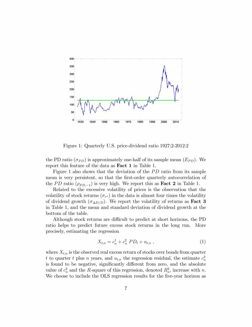
Figure 1: Quarterly U.S. price-dividend ratio 1927:2-2012:2

the PD ratio () is approximately one-half of its sample mean (). We

report this feature of the data as Fact 1 in Table 1.

Figure 1 also shows that the deviation of the ratio from its sample

mean is very persistent, so that the first-order quarterly autocorrelation of

the ratio (−1) is very high. We report this as Fact 2 in Table 1.Related to the excessive volatility of prices is the observation that the

volatility of stock returns () in the data is almost four times the volatility

of dividend growth (∆). We report the volatility of returns as Fact 3

in Table 1, and the mean and standard deviation of dividend growth at the

bottom of the table.

Although stock returns are difficult to predict at short horizons, the PD

ratio helps to predict future excess stock returns in the long run. More

precisely, estimating the regression

= 1 + 2 + (1)

where is the observed real excess return of stocks over bonds from quarter

to quarter plus years, and the regression residual, the estimate 2

is found to be negative, significantly different from zero, and the absolute

value of 2 and the -square of this regression, denoted 2, increase with .

We choose to include the OLS regression results for the five-year horizon as

7

Fact 4 in Table 1.6

Fact 1 Volatility of 123.91

PD ratio 62.43

Fact 2 Persistence of −1 0.97

PD ratio

Fact 3 Excessive return 11.44

volatility

Fact 4 Excess return 25 -0.0041

predictability 25 0.2102

Fact 5 Equity premium

Quarterly real stock returns 2.25

Quarterly real bond returns 0.15

Dividend Mean growth ∆

0.41

Behavior Std. dev. of growth ∆

2.88

PD ratio is price over quarterly dividend. Growth rates and returns

are expressed in real terms and at quarterly rates of increase.

Table 1: U.S. asset pricing facts 1927:2-2012:2

Finally, it is well known that through the lens of standard models, real

stock returns tend to be too high relative to short-term real bond returns,

a fact often referred to as the equity premium puzzle. We report it as Fact

6We focus on the five-year horizon for simplicity but obtain very similar results for

other horizons. Our focus on a single horizon is justified because chapter 20 in the work of

Cochrane (2005) shows that Facts 1, 2, and 4 are closely related: up to a linear approxima-

tion, the presence of return predictability and the increase in the 2 with the prediction

horizon are qualitatively a joint consequence of persistent PD ratios (Fact 2) and

dividend growth. It is not surprising, therefore, that our model also reproduces the in-

creasing size of 2 and 2 with We match the regression coefficients at the five-year

horizon to check the quantitative model implications.

8

5 in Table 1, which shows that the average quarterly real return on bonds

is much lower than the corresponding quarterly return on stocks

Table 1 reports ten statistics. As we show in section 5, we can replicate

these statistics using a model that has only four free parameters.

4 The Model

We describe below a Lucas (1978) asset pricing model with agents who hold

subjective prior beliefs about stock price behavior. We show that the presence

of subjective uncertainty implies that utility-maximizing agents update their

beliefs about stock price behavior using observed stock price realizations.7

Using a generic updating mechanism, section 4.2 shows that such learning

gives rise to oscillations of asset prices around their fundamental value and

qualitatively contributes to reconciling the Lucas asset pricing model with

the empirical evidence. Section 4.3 then introduces a specific system of prior

beliefs that gives rise to constant gain learning and that we employ in our

empirical work in section 5. Section 4.3 also shows under what conditions

this system of beliefs gives rise to small deviations from RE.

4.1 Model Description

The Environment: Consider an economy populated by a unit mass of

infinitely lived investors, endowed with one unit of a stock that can be traded

on a competitive stock market and that pays dividend consisting of a

perishable consumption good. Dividends evolve according to

−1= (2)

for = 0 1 2 where log ∼ N (−2

2 2) and ≥ 1. This implies

( ) = 1 ∆≡

³−−1−1

´= − 1 and 2∆

≡ ³−−1−1

´=

2³

2 − 1

´. To capture the fact that the empirically observed consumption

process is considerably less volatile than the dividend process and to replicate

the correlation between dividend and consumption growth, we assume that

each agent receives in addition an endowment of perishable consumption

7This draws on the results in the work of Adam and Marcet (2011).

9

goods. Total supply of consumption goods in the economy is then given by

the feasibility constraint = + . Following the consumption-based

asset pricing literature, we impose assumptions directly on the aggregate

consumption supply process8

−1= (3)

where log ∼ N (−22 2) and (log

log

) jointly normal. In our em-

pirical application, we follow the work of Campbell and Cochrane (1999)

and choose = 17 and the correlation between log and log

equal to

= 02.

Objective Function and Probability Space: Agent ∈ [0 1] has astandard time-separable expected utility function9

P0

∞X=0

(

)1−

1−

where ∈ (0∞) and denotes consumption demand of agent . The expec-

tation is taken using a subjective probability measure P that assigns prob-

abilities to all external variables (i.e., all payoff-relevant variables that are

beyond the agent’s control). Importantly, denotes the agent’s consump-

tion demand, and denotes the aggregate supply of consumption goods in

the economy.

The competitive stock market assumption and the exogeneity of the divi-

dend and income processes imply that investors consider the process for stock

prices and the income and dividends processes as exogenousto their decision problem. The underlying sample (or state) space Ω thus

consists of the space of realizations for prices, dividends, and income. Specif-

ically, a typical element ∈ Ω is an infinite sequence = ∞=0. Asusual, we let Ω denote the set of histories from period zero up to period

and its typical element. The underlying probability space is thus given

by (ΩB,P) with B denoting the corresponding -Algebra of Borel subsets

of Ω and P is the agent’s subjective probability measure over (ΩB).The probability measureP specifies the joint distribution of ∞=0

at all dates and is fixed at the outset. Although the measure is fixed, in-

8The process for is then implied by feasibility.9We assume standard preferences so as to highlight the effect of learning on asset price

volatility.

10

vestors’ beliefs about unknown parameters describing the stochastic processes

of these variables, as well as investors’ conditional expectations of future val-

ues of these variables, will change over time in a way that is derived from Pand that will depend on realized data. This specification thus encompasses

settings in which agents are learning about the stochastic processes describ-

ing and . Moreover, unlike in the anticipated utility framework

proposed in the work of Kreps (1998), agents are fully aware of the fact that

beliefs in the future will get revised. Although the probability measure Pis not equal to the distribution of ∞=0 implied by the model inequilibrium, it will be chosen in a way such that it is close to it in a sense

that we make precise in sections 4.3 and 6.3.

Expected utility is then defined as

P0

∞X=0

(

)1−

1− ≡ZΩ

∞X=0

(

)1−

1− P() (4)

Our specification of the probability space is more general than the one

used in other modeling approaches because we also include price histories in

the realization . Standard practice is to assume instead that agents know

the exact mapping (·) from a history of income and dividends to equi-

librium asset prices (), so that market prices carry only redundant

information. This allows us - without loss of generality - to exclude prices

from the underlying state space. This practice is standard in models of ra-

tional expectations, models with rational bubbles, in Bayesian RE models

such as those described in the second paragraph of section 2, and models

incorporating robustness concerns. This standard practice amounts to im-

posing a singularity in the joint density over prices, income, and dividends,

which is equivalent to assuming that agents know exactly the equilibrium

pricing function (·). Although a convenient modeling device, assumingexact knowledge of this function is at the same time very restrictive: it as-

sumes that agents have a very detailed knowledge of how prices are formed.

This makes it of interest to study the implication of (slightly) relaxing the

assumption that agents know the function (·). Adam and Marcet (2011)

show that rational behavior is indeed perfectly compatible with agents not

knowing the exact form of the equilibrium pricing function (·).1010Specifically, they show that with incomplete markets (i.e., in the absence of state-

contingent forward markets for stocks), agents cannot simply learn the equilibrium map-

11

Choice Set and Constraints: Agents make contingent plans for con-

sumption , bondholdings

and stockholdings

; that is, they choose the

functions ¡

¢: Ω → 3 (5)

for all ≥ 0. Agents’ choices are subject to the budget constraint +

+

≤ ( +)−1 + (1 + −1)

−1 + (6)

for all ≥ 0, where −1 denotes the real interest rate on riskless bonds issuedin period −1 and maturing in period . The initial endowments are given by−1 = 1 and

−1 = 0, so that bonds are in zero net supply. To avoid Ponzischemes and to ensure the existence of a maximum, the following bounds are

assumed to hold:

≤ ≤ (7)

≤ ≤

We only assume the bounds are finite and they satisfy 1

0 .

Maximizing Behavior (Internal Rationality): The investor’s prob-

lem then consists of choosing the sequence of functions

∞=0 to

maximize (4) subject to the budget constraint (6) and the asset limits (7),

where all constraints have to hold for all almost surely in P. Later on, theprobability measure P will be specified through some perceived law of mo-

tion describing the agent’s view about the evolution of ( ) over time,

together with a prior distribution about the parameters governing this law of

motion. Optimal behavior will then entail learning about these parameters,

in the sense that agents update their posterior beliefs about the unknown

parameters in the light of new price, income and dividend observations. For

the moment, this learning problem remains hidden in the belief structure P.Optimality Conditions: Since the objective function is concave and

the feasible set is convex, the agent’s optimal plan is characterized by the

first-order conditions¡

¢− = P

h¡+1

¢−+1

i+ P

h¡+1

¢−+1

i(8)¡

¢−= (1 + )

P

h¡+1

¢−i (9)

ping (·) by observing market prices. Furthermore, if the preferences and beliefs of agentsin the economy fail to be common knowledge, then agents cannot deduce the equilibrium

mapping from their own optimization conditions.

12

These conditions are standard except for the fact that the conditional expec-

tations are taken with respect to the subjective probability measure P.

4.2 Asset Pricing Implications: Analytical Results

This section presents analytical results that explain why the asset pricing

model with subjective beliefs can explain the asset pricing facts presented in

Table 1.

Before doing so, we briefly review the well-known result that under RE

the model is at odds with these asset pricing facts. A routine calculation

shows that the unique RE solution of the model is given by

=

1−1− 1−

(10)

where

= £(+1)

−+1¤

= (1+)22 −

The PD ratio is then constant, return volatility equals approximately the

volatility of dividend growth, and there is no (excess) return predictability,

so the model misses Facts 1 to 4 listed in Table 1. This holds independently of

the parameterization of the model. Furthermore, even for very high degrees

of relative risk aversion, say = 80, the model implies a fairly small risk pre-

mium. This emerges because of the low correlation between the innovations

to consumption growth and dividend growth in the data ( = 02).11 The

model thus also misses Fact 5 in Table 1.

We now characterize the equilibrium outcome under learning. One may be

tempted to argue that + can be substituted by + for = 0 1 in the first-

order conditions (8) and (9), simply because = holds in equilibrium

for all .12 However, outside of strict rational expectations we may have

11Under RE, the risk-free rate is given by 1+ =

µ−(1+)

22

¶−1and the expected

equity return equals [(+1 + +1)] = (−)−1. For = 0 there is thus no

equity premium, independently of the value for .12

= follows from market clearing and the fact that all agents are identical.

13

P

£+1

¤ 6= P [+1] even if in equilibrium

= holds ex post.13 To

understand how this arises, consider the following simple example. Suppose

agents know the aggregate process for and . In this case, P [+1]

is a function only of the exogenous variables ( ). At the same time,

P

£+1

¤is generally a function of price realizations also, since in the eyes

of the agent, optimal future consumption demand depends on future prices

and, therefore, also on today’s prices whenever agents are learning about price

behavior. As a result, in general P

£+1

¤ 6= P [+1], so that one cannot

routinely substitute individual by aggregate consumption on the right-hand

side of the agent’s first-order conditions (8) and (9).

Nevertheless, if in any given period the optimal plan for period +1 from

the viewpoint of the agent is such that¡+1(1−

+1)−+1

¢ ( +) is

expected to be small according to the agent’s expectations P then agents

with beliefs P realize in period that +1

≈ +1. This follows

from the flow budget constraint for period + 1 and the fact that = 1,

= 0, and

= in equilibrium in period . One can then rely on the

approximations

P

"µ+1

¶−(+1 ++1)

#' P

"µ+1

¶−(+1 ++1)

#(11)

P

"µ+1

¶−#' P

"µ+1

¶−# (12)

The following assumption provides sufficient conditions for this to be the

case:

Assumption 1 We assume that is sufficiently large and thatP +1

for some ∞ so that, given finite asset bounds the

approximations (11) and (12) hold with sufficient accuracy.

Intuitively, for high enough income , the agents’ asset trading decisions

matter little for the agents’ stochastic discount factor³+1

´−, allowing us

to approximate individual consumption in +1 by aggregate consumption in

13This is the case because the preferences and beliefs of agents are not assumed to be

common knowledge, so that agents do not know that = must hold in equilibrium.

14

+ 1.14 The bound on subjective price expectations imposed in Assumption

1 is justified by the fact that the price-dividend ratio will be bounded in equi-

librium, so that the objective expectation +1 will also be bounded.15

With Assumption 1, the risk-free interest rate solves

1 = (1 + )P

"µ+1

¶−# (13)

Furthermore, defining the subjective expectations of risk-adjusted stock price

growth

≡ P

õ+1

¶−+1

!(14)

and subjective expectations of risk-adjusted dividend growth

≡ P

õ+1

¶−+1

!

the first-order condition for stocks (8) implies that the equilibrium stock price

under subjective beliefs is given by

=1−

(15)

provided −1. The equilibrium stock price is thus increasing in (subjec-tive) expected risk-adjusted dividend growth and also increasing in expected

risk-adjusted price growth.

For the special case in which agents know the RE growth rates =

= 1− for all , equation (15) delivers the RE price outcome (10). Fur-thermore, when agents hold subjective beliefs about risk-adjusted dividend

growth but objectively rational beliefs about risk-adjusted price growth, then

= and (15) delivers the pricing implications derived in the Bayesian

RE asset pricing literature, as surveyed in section 2.

14Note that independent from their tightness, the asset holding constraints never prevent

agents from marginally trading or selling securities in any period along the equilibrium

path, where = 1 and = 0 holds for all .

15To see this, note that +1+1 implies [+1] ∞ where

denotes the mean dividend growth rate.

15

To highlight the fact that the improved empirical performance of the

present asset pricing model derives exclusively from the presence of subjective

beliefs about risk-adjusted price growth, we shall entertain assumptions that

are orthogonal to those made in the Bayesian RE literature. Specifically, we

assume that agents know the true process for risk-adjusted dividend growth:

Assumption 2 Agents know the process for risk-adjusted dividend growth,

that is, ≡ 1− for all .

Under this assumption, the asset pricing equation (15) simplifies to16

=1−1−

(16)

4.2.1 Stock Price Behavior under Learning

We now derive a number of analytical results regarding the behavior of asset

prices over time. We start out with a general observation about the volatility

of prices and thereafter derive results about the behavior of prices over time

for a general belief-updating scheme.

The asset pricing equation (16) implies that fluctuations in subjective

price expectations can contribute to the fluctuations in actual prices. As

long as the correlation between and the last dividend innovation is

small (as occurs for the updating schemes for that we consider in this

paper), equation (16) implies

µln

−1

¶'

µln1− −11−

¶+

µln

−1

¶ (17)

The previous equation shows that even small fluctuations in subjective price

growth expectations can significantly increase the variance of price growth,

and thus the variance of stock price returns, if fluctuates around values

close to but below −1.To determine the behavior of asset prices over time, one needs to take

a stand on how the subjective price expectations are updated over time.

16Some readers may be tempted to believe that entertaining subjective price beliefs while

entertaining objective beliefs about the dividend process is inconsistent with individual

rationality. Adam and Marcet (2011) show, however, that there exists no such contra-

diction, as long as the preferences and beliefs of agents in the economy are not common

knowledge.

16

To improve our understanding of the empirical performance of the model

and to illustrate that the results we obtain in our empirical application do

not depend on the specific belief system considered, we now derive analytical

results for a general nonlinear belief-updating scheme.

Given that denotes the subjective one-step-ahead expectation of risk-

adjusted stock price growth, it appears natural to assume that the measure

P implies that rational agents revise upward (downward) if they under-

predicted (overpredicted) the risk-adjusted stock price growth ex post. This

prompts us to consider measures P that imply updating rules of the form17

∆ =

õ−1−2

¶−−1−2

− −1; −1

!(18)

for given nonlinear updating functions : 2 → with the properties

(0;) = 0 (19)

(·;) increasing (20)

0 + (;) (21)

for all ( ) ∈ (0 ) and for some constant ∈ (1− −1). Prop-erties (19) and (20) imply that is adjusted in the same direction as the

last prediction error, where the strength of the adjustment may depend on

the current level of beliefs, as well as on calendar time (e.g., on the number

of observations available to date). Property (21) is needed to guarantee that

positive equilibrium prices solving (16) always exist.

In section 4.3 below we provide an explicit system of beliefs P in whichagents optimally update beliefs according to a special case of equation (18).

Updating rule (18) is more general and nests also other systems of beliefs, as

well as a range of learning schemes considered in the literature on adaptive

learning, such as the widely used least squares learning or switching gains

learning used by Marcet and Nicolini (2003).

To derive the equilibrium behavior of price expectations and price real-

izations over time, we first use (16) to determine realized price growth

−1=

µ+

∆1−

¶ (22)

17Note that is determined from observations up to period − 1 only. This simplifiesthe analysis and avoids simultaneity of price and forecast determination. This lag in the

information is common in the learning literature. Difficulties emerging with simultaneous

information sets in models of learning are discussed in the work of Adam (2003).

17

Combining the previous equation with the belief-updating rule (18), one

obtains

∆+1 = +1¡ (∆) (

)−

− ; ¢ (23)

where

(∆) ≡ 1− +1− ∆

1−

Given initial conditions (00 −1) and initial expectations 0, equation(23) completely characterizes the equilibrium evolution of the subjective price

expectations over time. Given that there is a one-to-one relationship

between and the PD ratio (see equation (16)), the previous equation also

characterizes the evolution of the equilibrium PD ratio under learning. High

(low) price growth expectations are thereby associated with high (low) values

for the equilibrium PD ratio.

The properties of the second-order difference equation (23) can be illus-

trated in a two-dimensional phase diagram for the dynamics of ( −1),which is shown in Figure 2 for the case in which the shocks ()

− assume

their unconditional mean value .18 The effects of different shock realiza-

tions for the dynamics will be discussed separately below.

The arrows in Figure 2 indicate the direction in which the vector ( −1)evolves over time according to equation (23), and the solid lines indicate the

boundaries of these areas.19 Since we have a difference equation rather than

a differential equation, we cannot plot the evolution of expectations exactly,

because the difference equation gives rise to discrete jumps in the vector

( −1) over time. Yet, if agents update beliefs only relatively weakly inresponse to forecast errors, as will be the case for our estimated model later

on, then for some areas in the figure, these jumps will be correspondingly

small, as we now explain.

Consider, for example, region A in the diagram. In this area −1and keeps decreasing, showing that there is momentum in price changes.

This holds true even if is already at or below its fundamental value 1−.

Provided the updating gain is small, beliefs in region Awill slowly move above

the 45 line in the direction of the lower left corner of the graph. Yet, once

they enter area B, starts increasing, so that in the next period, beliefs will

discretely jump into area . In region we have −1 and keeps

increasing, so that beliefs then display upward momentum. This manifests

18Appendix A.2 explains in detail the construction of the phase diagram.19The vertical solid line close to −1 is meant to illustrate the restriction −1.

18

B

A

t

t-1

t = t-1

a1-γρε (REE belief)

-1

t+1 = t

C

D

Figure 2: Phase diagram illustrating momentum and mean reversion

itself in an upward and rightward move of beliefs over time, until these reach

area . There, beliefs start decreasing, so that they move in one jump

back into area , thereby displaying mean reversion. The elliptic movements

of beliefs around 1− imply that expectations (and thus the PD ratio) arelikely to oscillate in sustained and persistent swings around the RE value.

The effect of the stochastic disturbances ()−

is to shift the curve

labeled “+1 = ” in Figure 2. Specifically, for realizations ()−

,

this curve is shifted upward. As a result, beliefs are more likely to increase,

which is the case for all points below this curve. Conversely, for ()−

, this curve shifts downward, making it more likely that beliefs decrease

from the current period to the next.

The previous results show that learning causes beliefs and the PD ratio

to stochastically oscillate around its RE value. Such behavior will be key in

explaining the observed volatility and the serial correlation of the PD ratio

(i.e., Facts 1 and 2 in Table 1). Also, from the discussion around equation

(17), it should be clear that such behavior makes stock returns more volatile

than dividend growth, which contributes to replicating Fact 3. As discussed

in the work of Cochrane (2005), a serially correlated and mean-reverting

19

PD ratio gives rise to excess return predictability, that is, it contributes to

matching Fact 4.

The momentum of changes in beliefs around the RE value of beliefs, as

well as the overall mean-reverting behavior, can be more formally captured

in the following results:

Momentum: If ∆ 0 and

≤ 1− ()−

, (24)

then ∆+1 0. This also holds if all inequalities are reversed.20

Therefore, up to a linear approximation of the updating function ,

−1[∆+1] 0

whenever ∆ 0 and ≤ 1− Therefore, beliefs have a tendency toincrease (decrease) further following an initial increase (decrease) whenever

beliefs are at or below (above) the RE value.

The following result shows formally that stock prices would eventually

return to their (deterministic) RE value in the absence of further disturbances

and that such reverting behavior occurs monotonically.21

Mean reversion: Consider an arbitrary initial belief ∈ (0 ). In theabsence of further disturbances ( + = + = 0 for all ≥ 0),

lim→∞

sup ≥ 1− ≥ lim→∞

inf

Furthermore, if 1− there is a period 0 ≥ such that is

nondecreasing between and 0 and nonincreasing between 0 and 00where 00 is the first period where 00 is arbitrarily close to 1− Sym-metrically, if 1−.

The previous result implies that - absent any shocks - cannot stay away

from the RE value forever. Beliefs either converge to the deterministic RE

value (when lim sup = lim inf) or stay fluctuating around it forever (when

20The result follows from the fact that condition (24) implies that the first argument in

the function on the right-hand side of equation (23) is positive.21See Appendix A.3 for the proof under an additional technical assumption.

20

lim sup lim inf). Any initial deviation, however, is eventually eliminated

with the reversion process being monotonic. This result also implies that an

upper bound on price beliefs cannot be an absorbing point: if beliefs go

up and they get close to the upper bound , they will eventually bounce

off this upper bound and go back down toward the RE value.

Summing up, the previous results show that for a general set of belief-

updating rules, stock prices and beliefs fluctuate around their RE values in

a way that helps to qualitatively account for Facts 1 to 4 listed in Table 1.

4.3 Optimal Belief Updating: Constant Gain Learning

We now introduce a fully specified probability measure P and derive the

optimal belief-updating equation it implies. We employ this belief-updating

equation in our empirical work in section 5. We show below a precise sense

in which this system of beliefs represents a small deviation from RE.

In line with Assumption 2, we consider agents who hold rational expecta-

tions about the dividend and aggregate consumption processes. At the same

time, we allow for subjective beliefs about risk-adjusted stock price growth

by allowing agents to entertain the possibility that risk-adjusted price growth

may contain a small and persistent time-varying component. This is moti-

vated by the observation that in the data there are periods in which the PD

ratio increases persistently, as well as periods in which the PD ratio falls per-

sistently (see Figure 1). In an environment with unpredictable innovations

to dividend growth, this implies the existence of persistent and time-varying

components in stock price growth. For this reason, we consider agents who

think that the process for risk-adjusted stock price growth is the sum of a

persistent component and of a transitory component µ

−1

¶−

−1= + (25)

= −1 +

for ∼ (0 2), ∼ (0 2), independent of each other and also

jointly i.i.d. with and .22 The latter implies [( ) |−1] = 0, where

−1 includes all the variables in the agents’ information set at −1, includingall prices, endowments, and dividends dated − 1 or earlier.22Notice that we use the notation = + , so that equation (25) contains only

payoff-relevant variables that are beyond the agent’s control.

21

The previous setup encompasses the RE equilibrium beliefs as a special

case. Namely, when agents believe 2 = 0 and assign probability one to

0 = 1−, we have that = 1− for all ≥ 0 and prices are as givenby RE equilibrium prices in all periods.

In what follows we allow for a nonzero variance 2, that is, for the pres-

ence of a persistent time-varying component in price growth. The setup then

gives rise to a learning problem because agents observe only the realizations

of risk-adjusted price growth, but not the persistent and transitory compo-

nent separately. The learning problem consists of optimally filtering out the

persistent component of price growth . Assuming that agents’ prior beliefs

0 are centered at the RE value and given by

0 ∼ (1− 20)

and setting 20 equal to the steady state Kalman filter uncertainty about ,

which is given by

20 =−2 +

q¡2¢2+ 42

2

2

agents’ posterior beliefs at any time are given by

∼ ( 0)

with optimal updating implying that , defined in equation (14), recursively

evolves according to

= −1 +1

õ−1−2

¶−−1−2

− −1

! (26)

The optimal (Kalman) gain is given by 1 =¡20 + 2

¢¡20 + 2 + 2

¢and

captures the strength with which agents optimally update their posteriors in

response to surprises.23

These beliefs constitute a small deviation from RE beliefs in the limit-

ing case with vanishing innovations to the random walk process (2 → 0).

23In line with equation (18), we incorporate information with a lag, so as to eliminate

the simultaneity between prices and price growth expectations. The lag in the updating

equation could be justified by a specific information structure where agents observe some

of the lagged transitory shocks to risk-adjusted stock price growth.

22

Agents’ prior uncertainty then vanishes (20 → 0), and the optimal gain con-

verges to zero (1 → 0). As a result, → 1− in distribution for all ,so that one recovers the RE equilibrium value for risk-adjusted price growth

expectations. This shows that for a given distribution of asset price, agents’

beliefs are close to RE beliefs for a small value of the gain parameter (1).24

For our empirical application, we need to slightly modify the updating

equation (26) to guarantee that the bound holds for all periods

and equilibrium prices always exist. The exact way in which this bound

is imposed matters little for our empirical result, because the moments we

compute do not change much as long as is close to only rarely over

the sample length considered. To impose this bound, we consider in our

empirical application a concave, increasing, and differentiable function :

+ → (0 ) and modify the belief-updating equation (26) to25

=

Ã−1 +

1

"µ−1−2

¶−−1−2

− −1

#! (27)

where

() = if ∈ (0 )for some ∈ (1− ). Beliefs thus continue to evolve according to(26), as long as they are below the threshold , whereas for higher beliefs

we have that () ≤ . The modified algorithm (27) satisfies the constraint

(21) and can be interpreted as an approximate implementation of a Bayesian

updating scheme where agents have a truncated prior that puts probability

zero on .26,27

24We show below that continues to be true when using the equilibrium distribution of

asset prices generated by these beliefs.25The exact functional form for that we use in the estimation is shown in appendix

A.5.26The issue of bounding beliefs so as to ensure that expected utility remains finite

is present in many applications of both Bayesian and adaptive learning to asset prices.

The literature has typically dealt with this issue by using a projection facility, assuming

that agents simply ignore observations that would imply updating beliefs beyond the

required bound. See the work of Timmermann (1993, 1996), Marcet and Sargent (1989),

or Evans and Honkapohja (2001). This approach has two problems. First, it does not arise

from Bayesian updating. Second, it introduces a discontinuity in the simulated moments

and creates difficulties for our MSM estimation in section 5, prompting us to pursue the

differentiable approach to bounding beliefs described above.27Adam, Beutel, and Marcet (2014) solve the model without Assumption 1, which is

23

We now show that for a small value of the gain (1), agents’ beliefs

are close to RE beliefs when using the equilibrium distribution of prices

generated by these beliefs. More precisely, the setup gives rise to a stationary

and ergodic equilibrium outcome in which risk-adjusted stock price growth

expectations have a distribution that is increasingly centered at the RE value

1− as the gain parameter becomes vanishingly small. From equation

(16), it then follows that actual equilibrium prices also become increasingly

concentrated at their RE value, so that the difference between beliefs and

outcomes becomes vanishingly small as 1→ 0.

Stationarity, Ergodicity, and Small Deviations from RE: Suppose agents’

posterior beliefs evolve according to equation (27) and equilibrium prices

are determined according to equation (16). Then is geometrically

ergodic for sufficiently large . Furthermore, as 1 → 0 we have

[]→ 1− and ()→ 0.

The proof is based on results from the work of Duffie and Singleton (1993)

and contained in appendix A.4. Geometric ergodicity implies the existence

of a unique stationary distribution for that is ergodic and that is reached

from any initial condition. Geometric ergodicity is required for estimation

by MSM.

We explore further in section 6 the connection between agents’ beliefs and

model outcomes.

5 Quantitative Model Performance

This section evaluates the quantitative performance of the asset pricing model

with subjective price beliefs and shows that it can robustly replicate Facts 1 to

4 listed in Table 1. We formally estimate and test the model using the method

of simulated moments (MSM). This approach to structural estimation and

testing helps us to focus on the ability of the model to explain the specific

computationally much more costly, so that one cannot use MSM to estimate the model.

They use the optimal consumption plan that solves the individual investor’s problem to

price the asset and show how a projection facility then arises endogenously from the wealth

effect in the standard case that relative risk aversion is larger than one.

24

moments of the data described in Table 1.28 Regarding Fact 5 in Table 1,

the model gives rise to an equity premium that is much higher than under

RE, but for reasonable degrees of relative risk aversion, it tends to fall short

of the risk premium observed in the data.

We first evaluate the model’s ability to explain the individual moments,

which is the focus of much of the literature on matching stock price volatility.

We find that the model can explain the individual moments well. Using

-statistics based on formal asymptotic distribution, we find that in some

versions of the model, all -statistics are at or below 2 in absolute value, even

with a moderate relative risk aversion of = 5. Moreover, with this degree

of risk aversion, the model can explain up to 50% of the equity premium.

We then turn to the more demanding task of testing if all the moments

are accepted jointly by computing chi-square test statistics. Due to their

stringency, such test statistics are rarely reported in the consumption-based

asset pricing literature. A notable exception is the work of Bansal, Kiku,

and Yaron (2013), who test the overidentifying restrictions of a long-run risk

model. Different from our approach, they test equilibrium conditions instead

of matching statistics. Also, they use a diagonal weighting matrix instead

of the optimal weighting matrix in the objective function (29) introduced

below.

We find that with a relative risk aversion of = 5, the model fails to pass

an overall goodness of fit as long as one includes the equity premium. Yet,

the test reaches a moderate -value of 2.5% once we exclude the risk-free

rate from the set of moments to be matched, confirming that it is the equity

premium that poses a quantitative challenge to the model.29 With a relative

risk aversion of = 3, the -value increases even further to 7.1% when we

again exclude the risk-free rate.

28A popular alternative approach in the asset pricing literature has been to test if

agents’ first-order conditions hold in the data. Hansen and Singleton (1982) pioneered

this approach for RE models, and Bossaerts (2004) provides an approach that can be

applied to models of learning. We pursue the MSM estimation approach here because it

naturally provides additional information on how the formal test for goodness of fit of the

model relates to the model’s ability to match the moments of interest. The results are

then easily interpretable; they point out which parts of the model fit well and which parts

do not, thus providing intuition about possible avenues for improving the model fit.29The literature suggests a number of other model ingredients, that - once added -

would allow generating a higher equity premium. See, for example, ambiguity aversion as

in Collard et al. (2011), initially pessimistic expectations as in Cogley and Sargent (2008),

or habits in consumption preferences.

25

Finally, we allow for a very high risk aversion coefficient. Specifically, we

set = 80, which is the steady state value of relative risk aversion used in

Campbell and Cochrane (1999).30 The model then replicates all moments

in Table 1, including the risk premium. In particular, the model generates

a quarterly equity premium of 2.0%, slightly below the 2.1% per quarter

observed in U.S. data, while still replicating all other asset pricing moments.

The next section explains the MSM approach for estimating the model

and the formal statistical test for evaluating the goodness of fit. The subse-

quent section reports on the estimation and test outcomes.

5.1 MSM Estimation and Statistical Test

This section outlines the MSM approach and the formal test for evaluating

the fit of the model. This is a simple adaptation of standard MSM to include

matching of statistics that are functions of simple moments by using the delta

method (see appendix A.6 for details).

For a given value of the coefficient of relative risk aversion, there are four

free parameters left in the model, comprising the discount factor , the gain

parameter 1, and the mean and standard deviation of dividend growth,

denoted by and ∆, respectively. We summarize these in the parameter

vector

≡³ 1 ∆

´

The four parameters will be chosen so as to match some or all of the ten

sample moments in Table 1:31³ b b b b b−1 b52 b25 b b∆ b∆

´ (28)

Let bS ∈ denote the subset of sample moments in (28) that will be

matched in the estimation, with denoting the sample size and ≤ 10.3230This value is reported on page 244 in their paper.31Many elements listed in (28) are not sample moments, but they are nonlinear functions

of sample moments. For example, the 2 coefficient is a function of sample moments. This

means we have to use the delta method to adapt standard MSM (see appendix A.6). It

would be more precise to refer to the elements in (28) as “sample statistics,” as we do in

the appendix. For simplicity, we avoid this terminology in the main text.32As discussed before, we exclude the risk premium from some estimations; in those

cases, 10

26

Furthermore, let eS() denote the moments implied by the model for someparameter value . The MSM parameter estimate b is defined as

b ≡ argmin

h bS − eS()i0 bΣ−1S h bS − eS()i (29)

where bΣS is an estimate of the variance-covariance matrix of the sample

moments bS . The MSM estimate b chooses the model parameter such thatthe model moments eS() fit the observed moments bS as closely as possiblein terms of a quadratic form with weighting matrix bΣ−1S . We estimate bΣSfrom the data in a standard way. Adapting standard results from MSM, one

can prove that for a given list of moments included in bS , the estimate bis consistent and is the best estimate among those obtained with different

weighting matrices.

The MSM estimation approach also provides an overall test of the model.

Under the null hypothesis that the model is correct, we have

c ≡ h bS − eS(b)i0 bΣ−1S h bS − eS(b)i→ 2−4 as →∞ (30)

where convergence is in distribution. Furthermore, we obtain a proper

asymptotic distribution for each element of the deviations bS− eS(b) so thatwe can build -statistics that indicate which moments are better matched in

the estimation.

In our application we find a nearly singular bΣS . As shown in appen-dix A.6, asymptotic results require this matrix to be invertible. The near-

singularity indicates that one statistic is nearly redundant (i.e., carries prac-

tically no additional information). The appendix describes a procedure for

selecting the redundant statistic; it suggests that we drop the coefficient from

the five-year-ahead excess return regression b52 from the estimation. In the

empirical section below, the value of the regression coefficient implied by the

estimated model is always such that the -statistic for this moment remains

below 2. This happens even though information about b52 has not been usedin the estimation.

5.2 Estimation Results

Table 2 reports estimation outcomes when assuming = 5. The second and

third columns in the table report the asset pricing moments from the data

27

and the estimated standard deviation for each of these moments, respectively.

Columns 4 and 5 then show the model moments and the -statistics, respec-

tively, when estimating the model using all asset pricing moments (except for

52, which has been excluded for reasons explained in the previous section).

All estimations impose the restriction ≤ 1.The estimated model reported in columns 4 and 5 of Table 2 quantita-

tively replicates the volatility of stock returns (), the large volatility and

high persistence of the PD ratio ( −1), as well as the excess returnpredictability evidence (25

25). This is a remarkable outcome given the as-

sumed time-separable preference structure. The model has some difficulty in

replicating the mean stock return and dividend growth, but -statistics for

all other moments have an absolute value well below 2, and more than half

of the -statistics are below 1.

U.S. data Estimated model Estimated model

(52 not included) (52, not included)

Data Std. Model Model

Moment dev. moment -stat. moment -stat.bS b S eS(b) eS(b)Quarterly mean stock return 2.25 0.34 1.27 2.70 1.49 2.06

Quarterly mean bond return 0.15 0.19 0.39 -1.27 0.49 -1.78

Mean PD ratio 123.91 21.36 122.50 0.07 119.05 0.23

Std. dev. stock return 11.44 2.71 10.85 0.22 11.60 -0.06

Std. dev. PD ratio 62.43 17.60 67.55 -0.29 69.59 -0.41

Autocorrel. PD ratio −1 0.97 0.01 0.95 0.62 0.95 0.84

Excess return reg. coefficient 25 -0.0041 0.0014 -0.0066 1.79 -0.0067 1.90

2 of excess return regression 25 0.2102 0.0825 0.2132 -0.04 0.1995 0.13

Mean dividend growth ∆ 0.41 0.17 0.00 2.79 0.10 1.82

Std. dev. dividend growth ∆ 2.88 0.82 2.37 0.61 2.45 0.52

Discount factor b 0.9959 1.0000

Gain coefficient 1b 0.0073 0.0076

Test statistic c 82.6 62.6

-value c 0.0% 0.0%

Table 2: Estimation outcome for = 5

The last two columns in Table 2 report the estimation outcome when

28

dropping the mean stock return from the estimation and restricting to 1,

which tends to improve the ability of the model to match individual moments.

All -statistics are then close to or below 2, including the -statistics for the

mean stock return and for 52 that have not been used in the estimation, and

the majority of the -statistics are below 1. This estimation outcome shows

that the subjective beliefs model successfully matches individual moments

with a relatively low degree of risk aversion. The model also delivers an

equity premium of 1% per quarter, that is, nearly half of the value observed

in U.S. data (2.1% per quarter).

The measure for the overall goodness of fitc and its -value are reported

in the last two rows of Table 2. The statistic is computed using all moments

that are included in the estimation. The reported values of c are off the

chart of the 2 distribution, implying that the overall fit of the model is

rejected, even if all moments are matched individually.33 This indicates that

some of the joint deviations observed in the data are unlikely to happen given

the observed second moments. It also shows that the overall goodness of fit

test is considerably more stringent.

To show that the equity premium is indeed the source of the difficulty for

passing the overall test, columns 4 and 5 in Table 3 report results obtained

when we repeat the estimation excluding the risk-free rate instead of the

stock returns from the estimation. The estimation imposes the constraintb ≤ 1, since most economists believe that values above 1 are unacceptable.This constraint turns out to be binding. The -statistics for the individual

moments included in the estimation are then quite low, but the model fails

to replicate the low value for the bond return , which has not been used in

the estimation. Despite larger -statistics, the model now comfortably passes

the overall goodness of fit test at the 1% level, as the -value for the reportedc =12.87 statistic is 2.5%. The last two columns in Table 3 repeat the

estimation when imposing = 3 and b = 1. The performance in terms ofmatching the moments is then very similar with = 5, but the -value of

the c statistic increases to 7.1%.

Figure 3 shows realizations of the time series outcomes for the PD ratio

generated from simulating the estimated model from Table 3 with = 5, for

33The 2 distribution has 5 degrees of freedom for the estimations in Table 2, where

the last two columns drop a moment but also fix = 1. For the estimation in Table 3,

we exclude 52 and from the estimation, but the constraint b ≤ 1 is either binding

or imposed, so that we also have 5 degrees of freedom. Similarly, we have 5 degrees of

freedom for the estimation in Table 4.

29

the same number of quarters as numbers of observations in our data sample.

The simulated time series display price booms and busts, similar to the ones

displayed in Figure 1 for the actual data, so that the model also passes an

informal “eyeball test.”

The estimated gain coefficients in Tables 2 and 3 are fairly small. The

estimate in Table 3 implies that agents’ risk-adjusted return expectations

respond only 07% in the direction of the last observed forecast error, sug-

gesting that the system of price beliefs in our model indeed represents only

a small deviation from RE beliefs. Under strict RE, the reaction to forecast

errors is zero, but the model then provides a very bad match with the data:

it counterfactually implies ≈ ∆, = 0, and 25 = 0.

U.S. data Estimated model Estimated model

= 5 = 3

(52, not included) (52, not included)

Data Model Model

moment moment -stat. moment -stat.bSeS(b) eS(b)

Quarterly mean stock return 2.25 1.32 2.50 1.51 2.00

Quarterly mean bond return 0.15 1.09 -4.90 1.30 -5.98

Mean PD ratio 123.91 109.66 0.69 111.28 0.58

Std. dev. stock return 11.44 5.34 2.25 5.10 2.33

Std. dev. PD ratio 62.43 40.09 1.33 39.11 1.31

Autocorrel. PD ratio −1 0.97 0.96 0.30 0.96 0.23

Excess return reg. coefficient 25 -0.0041 -0.0050 0.64 -0.0050 0.60

2 of excess return regression 25 0.2102 0.2282 -0.22 0.2302 -0.24

Mean dividend growth ∆ 0.41 0.22 1.14 0.43 -0.09

Std. dev. dividend growth ∆ 2.88 1.28 1.95 1.23 2.00

Discount factor b 1.0000 1.0000

Gain coefficient 1b 0.0072 0.0071

Test statistic c 12.87 11.07

-value of c 2.5% 7.1%

Table 3: Estimation outcome for = 5 and = 3

To further examine what it takes to match the risk premium and to com-

pare more carefully our results with the performance of other models in the

30

literature, we now assume a high degree of risk aversion of = 80, in line

with the steady state degree of risk aversion assumed in the work of Camp-

bell and Cochrane (1999). Furthermore, we use all asset pricing moments

listed in equation (28) for estimation, except for 52. The estimation results

are reported in Table 4. The learning model then successfully replicates all

moments in the data, including the risk premium: all the -statistics for the

individual moments are below 2 in absolute value, with most of them even

assuming values below 1. For sufficiently high risk aversion, we thus match

all individual moments, so that the model performance is comparable to that

of Campbell and Cochrane (1999) but achieved with a time-separable pref-

erence specification. Yet, the -value for the test statistic c in Table 4 is

again off the charts, implying that the model fails the overall goodness of fit

test. This highlights that the c test statistic is a much stricter test than

imposed by matching moments individually.

U.S. data Estimated model

(52 not included)

Data Model

moment moment -stat.bSeS(b)

Quarterly mean stock return 2.25 2.11 0.40

Quarterly mean bond return 0.15 0.11 0.21

Mean PD ratio 123.91 115.75 0.38

Std. dev. stock return 11.44 16.31 -1.80

Std. dev. PD ratio 62.43 71.15 -0.50

Autocorrel. PD ratio −1 0.97 0.95 1.13

Excess return reg. coefficient 25 -0.0041 -0.0061 1.39

2 of excess return regression 25 0.2102 0.2523 -0.51

Mean dividend growth ∆ 0.41 0.16 1.50

Std. dev. dividend growth ∆ 2.88 4.41 1.86

Discount factor b 0.998

Gain coefficient 1b 0.0021

Test statistic c 28.8

-value of c 0.0%

Table 4: Estimation outcome for = 80

31

Figure 3: Simulated PD ratio, estimated model from Table 3 ( = 5)

32

Interestingly, the learning model gives rise to a significantly larger risk

premium than its RE counterpart.34 For the estimated parameter values in

Table 4, the quarterly real risk premium under RE is less than 0.5%, which

falls short of the 2.0% emerging in the model with learning.35 Surprisingly,

the model generates a small, positive ex post risk premium for stocks even

when investors are risk neutral ( = 0). This finding may be surprising, since

we did not introduce any feature in the model to generate a risk premium.

To understand why this occurs, note that the realized gross stock return

between period 0 and period can be written as the product of three terms:

Y=1

+

−1=

Y=1

−1| z =1

·µ + 1

0

¶| z

=2

·−1Y=1

+ 1

| z =3

The first term (1) is independent of the way prices are formed and thus

cannot contribute to explaining the emergence of an equity premium in the

model with learning. The second term (2), which is the ratio of the terminal

over the starting value of the PD ratio, could potentially generate an equity

premium but is on average below 1 in our simulations of the learning model,

whereas it is slightly larger than 1 under RE.36 The equity premium in the

learning model must thus be due to the last component (3). This term is

convex in the PD ratio, so that a model that generates higher volatility of

the PD ratio (but the same mean value) will also give rise to a higher equity

premium. Therefore, because our learning model generates a considerably

more volatile PD ratio, it also gives rise to a larger ex post risk premium.

6 Robustness of Results

This section discusses the robustness of our findings with regard to different

learning specifications and parameter choices (section 6.1), analyzes in detail

the extent to which agents’ forecasts could be rejected by the data or the

34The RE counterpart is the model with the same parameterization, except for 1 = 0.35The learning model and the RE model imply the same risk-free rate, because we

assumed that agents have objective beliefs about the aggregate consumption and dividend

process.36For the learning model, we choose the RE-PD ratio as our starting value.

33

equilibrium outcomes of the model (section 6.2), and finally offers a discus-

sion of the rationality of agents’ expectations about their own future choices

(section 6.3).

6.1 Different Parameters and Learning Specifications

We explored the robustness of the model along a number of dimensions.

Performance turns out to be robust as long as agents are learning in some

way about price growth using past price growth observations. For example,

Adam, Beutel, and Marcet (2014) use a model in which agents learn directly

about price growth (without risk adjustment) using observations of past price

growth; they document a very similar quantitative performance. Adam and

Marcet (2010) considered learning about returns using past observations of

returns, showing how this leads to asset price booms and busts. Further-

more, within the setting analyzed in the present paper, results are robust to

relaxing Assumption 2. For example, the asset pricing moments are virtually

unchanged when considering agents who also learn about risk-adjusted div-

idend growth, using the same weight 1 for the learning mechanism as for

risk-adjusted price growth rates. Indeed, given the estimated gain parame-

ter, adding learning about risk-adjusted dividend growth contributes close

to nothing to replicating stock price volatility. We also explored a model

of learning about risk-adjusted price growth that switches between ordinary

least squares learning and constant gain learning, as in the work of Marcet

and Nicolini (2003). Again, model performance turns out to be robust. Taken

together, these findings suggest that the model continues to deliver an empir-

ically appealing fit, as long as expected capital gains are positively affected

by past observations of capital gains.

The model fails to deliver a good fit with the data if one assumes that

agents learn only about the relationship between prices and dividends, say

about the coefficient in front of in the RE pricing equation (10), using

the past observed relationship between prices and dividends (see the work

of Timmermann (1996)). Stock price volatility then drops significantly be-

low that observed in the data, illustrating that the asset pricing results are

sensitive to the kind of learning introduced in the model. Our finding is

that introducing uncertainty about the growth rate of prices is key for un-

derstanding asset price volatility.

Similarly, for lower degrees of relative risk aversion around 2, we find that

the model continues to generate substantial volatility in stock prices but not

34

enough to quantitatively match the data.

At the same time, it is not difficult to obtain an even better fit than

the one reported in section 5.2. For example, we imposed the restrictionb ≤ 1 in the estimations reported in Table 3. Yet, in a setting with outputgrowth and uncertainty, values above 1 are easily compatible with a well-

defined model and positive real interest rates. Reestimating Table 3 for

= 5 without imposing the restriction on the discount factor, one obtainsb =1.0094 and a -value of 4.3% for the overall fit instead of the 2.5%

reported. The fit could similarly be improved by changing the parameters

of the projection facility. Choosing¡

¢= (200 400) for the estimation

in Table 3 with = 5 instead of the baseline values¡

¢= (250 500)

raises the -value from 2.5% to 3.1%.37

6.2 Testing for the Rationality of Price Expectations

In section 4.3 we presented limiting results that guarantee that agents’ beliefs

constitute only a small deviation from RE, in the sense that for an arbitrarily

small gain, agents’ beliefs are close to the beliefs of agents in a rational

expectations model. This section studies to what extent agents could discover

that their system of beliefs is not exactly correct by observing processes for

( ).38 We study this for the beliefs implied by the estimated models

from section 5.1.

In a first step, we derive a set of testable restrictions implied by agents’

beliefs system (2), (3), and (25). Importantly, under standard assumptions,

any process satisfying these testable restrictions can - in terms of its auto-

covariance function - be generated by the postulated system of beliefs. The

set of derived restrictions thus fully characterizes the second-moment impli-

cations of the beliefs system.

In a second step, we test the derived restrictions against the data. We

show that the data uniformly accept all testable second-order restrictions.

This continues to be the case when we consider certain higher-order or non-

linear tests that go beyond second-moment implications. Based on this, we

can conclude that the agents’ belief system is reasonable: given the behavior

of actual data, the belief system is one that agents could have entertained.

37Choosing³

´= (300 600) causes the p-value to decrease to 1.8%.

38Here, denotes aggregate consumption, that is, = −, which agents take as

given.

35

In a third step, we test the derived restrictions against simulated model

data. Again, we find that the restrictions are often accepted in line with the

significance level of the test, although for some of the models and some of the

tests, we obtain more rejections than implied by the significance level, espe-

cially when considering longer samples of artificial data. Since the testable

implications are accepted by the actual data, rejections obtained from simu-

lated data indicate areas in which the asset pricing model could be improved

further.

6.2.1 Testable Restrictions

In order to routinely use asymptotic theory, we transform the variables into

stationary ones and consider the joint implications of the belief system (2),

(3), and (25) for the vector = ( −1 −1), where

≡ ∆

µ

−1

¶−

−1 (31)

with∆ denoting the difference operator.39 The following proposition presents

a set of testable restrictions about .40

Proposition 1 (Necessity of Restrictions 1-4) If follows the sys-tem of beliefs (2), (3), and (25), then

Restriction 1 : (−) = 0 for all ≥ 2Restriction 2 :

µµ

−1+

−1−2

−1+

−1−2

¶

¶= 0

Restriction 3 : 0 Σ +( −1) 0

Restriction 4 : () = 0

39One might be tempted to test (31) using an augmented Dickey-Fuller (ADF) test,

which involves running a regression with a certain number of lags, and test if the residual is

serially correlated. This approach is problematic in our application: as shown in appendix

A.7, we have = −−1+ ; since the gain is small in the estimates in Tables 2 - 4, we

also have that 22 is small, so that the MA representation of has a near unit root. In

this case, the true autoregressive representation of ∆³

−1

´−−1

has coefficients that

decay very slowly with the lag length. The ADF test then does not work: if we introduce

only a few lags into the regression, then the error would be serially correlated and the test

would be asymptotically invalid; if we introduce many lags, then the test has little power

for reasonable sample lengths.40Appendix A.7 provides a proof.

36

where Σ ≡ ³

−1 −1

´and ≡ Σ−1

∙³

−1 −1

´0

¸.

Given standard assumptions entertained in the asset pricing literature, it

turns out that Restrictions 1-4 in the previous proposition are also sufficient

for to be consistent with the belief system in terms of second-moment

implications. In particular, suppose the following holds:

Assumption 3 (i) is second-order stationary; (ii)³

−1 −1

´is serially

uncorrelated and ³

−1

´=

³

−1

´; (iii)

³

−1 −1

´is uncorre-

lated with − for all 1.

Conditions (i)-(iii) in the previous assumption hold true in our asset pric-

ing model. We do not question their validity when testing the belief system

using actual data, because they are working assumptions maintained by much

of the consumption-based asset pricing literature. Appendix A.7 then proves

the following result:

Proposition 2 (Sufficiency of Restrictions 1-4) Suppose the stochastic

process satisfies Assumption 3. If this process also satisfies Restrictions1-4 stated in Proposition 1, then there exists a belief system of the form (2),

(3), and (25), whose autocovariance function is identical to that of .

The proposition shows that - conditional on Assumption 3 being satisfied

- any process satisfying Restrictions 1-4 in Proposition 1 can - in terms of its

second-moment implications - be generated from the belief system.

One can derive further higher moment implications from the belief system,

based on the observation that in equation (31) has an MA(1) structure,

as we show in appendix A.7, and that all variables in the belief system are

jointly normally distributed. Under normality, the absence of serial correla-

tion implies independence, so that we have

[−] = 0 (32)

where − can be any stationary nonlinear transformation of variables con-tained in the − information set of agents with ≥ 2. Obviously, due tothe large number of possible instruments −, it is impossible to provide anexhaustive test of (32). We thus simply report tests of (32) based on some

natural instruments −.

37

We test the moment restrictions from Proposition 1 in a standard way,

as described in detail in appendix A.8. Testing Restriction 1 involves an

infinite number of variables and therefore requires some discretionary choice

regarding the set of instruments. We proceed by running separate tests with

each of the three elements in −2, also including a constant and three lagsof the considered element.41

6.2.2 Testing Beliefs Against Actual Data

Table 5 reports the test statistics when testing Restrictions 1-4 from Propo-

sition 1 using actual data. We compute risk-adjusted consumption growth in

the data assuming = 5 (second column) and = 80 (third column).42 The

5% critical value of the test statistic is reported in the last column of Table

5. The table shows that the test statistic is in all cases below its critical

value and often so by a wide margin. It then follows from Proposition 2 that

agents find the observed asset pricing data, in terms of second moments, to

be compatible with their belief system.

Test statistic Test statistic 5% critical

= 5 = 80 value

Restriction 1 using−

−−16.69 3.10 9.48

Restriction 1 using−

−−13.47 0.80 9.48

Restriction 1 using ∆³

−−−1

´−−

−−16.97 1.38 9.48

Restriction 2 0.28 4.31 5.99

Restriction 3 -7.15 -2.96 1.64

Restriction 4 0.01 0.11 3.84

Table 5: Empirical test of P based on Proposition 1

Table 6 presents further tests based on equation (32) using natural non-

linear transformations of the variables −, namely, past PD ratio and past

41We also performed joint tests that include as instruments a constant, the entire vector

−2, and three lags of the vector. This leads to very similar conclusions, but in case of arejection is less informative about which element in delivers the rejection.42We use the consumption data provided by Campbell and Cochrane (1999), which is

available for the period 1947-1994.

38

price growth. As before, tests include a constant and three lags of the stated

variable. Test statistics are again below the 5% critical value in all cases.

Taken together with the evidence from Table 5, this shows that agents’ belief

system is a reasonable one to hold, given the way the data actually behaved.

Test statistic Test statistic 5% critical

Instrument = 5 = 80 value−−

6.33 2.90 9.48−

−−14.68 4.50 9.48

Table 6: Empirical test of P, additional instruments

6.2.3 Testing Beliefs Against Simulated Data

Table 7 reports the rejection frequencies for Restriction 1 when using simu-

lated model data.43 Specifically, the table reports the likelihood of rejecting

Restriction 1 at the 5% significance level, using simulated data based on the

point estimates from Table 3 ( = 5) and the point estimates from Table 4

( = 80). Rejection frequencies are shown for different instruments, different

sample lengths of simulated quarterly data, and different numbers of lags

in the tests. The longest sample length corresponds to the length of the data

sample.

Obviously, one cannot expect that this test is never rejected. Even the

correct model would be rejected because of Type I errors (i.e., about 5% of

the time). One can evaluate agents’ subjective beliefs within the model by

checking whether the rejection frequencies exceed the 5% significance level.

Table 7 shows that with 60 to 100 quarters of simulated data, the rejection

frequencies for the different tests considered are about as many times below

the 5% level as they are above this level. With 200 or 340 quarters of data,

the rejection rates are higher for the dividend growth instruments using pa-

rameters from Table 3 and for risk-adjusted price and consumption growth

for the model from Table 4. This indicates that these variables may help

to improve agents’ forecasts within the model. Yet, given that these same

43The rejection frequencies are obtained from simulating 1,000 random samples of the

specified length.

39

tests are not rejected when using actual data, these rejection rates suggest

dimensions along which the model could be further improved.

Model from Table 3, = 5 Model from Table 4

Instrument lags\T: 60 100 200 340 60 100 200 340−

−−11 5.0% 6.9% 13.5% 19.6% 1.7% 2.1% 2.5% 1.4%

3 4.9% 9.7% 18.5% 26.2% 3.6% 3.7% 3.4% 2.8%−

−−11 2.3% 3.7% 6.0% 5.8% 10.3% 18.7% 29.0% 44.0%

3 5.3% 5.7% 9.9% 11.3% 12.0% 21.3% 38.0% 56.7%

∆³

−−−1

´−−

−−11 1.8% 1.9% 1.3% 0.8% 5.8% 10.9% 13.8% 18.5%

3 4.3% 4.6% 9.0% 16.0% 9.0% 12.6% 25.1% 36.5%

Rejection frequency at 5% significance level

Table 7: Test of Restriction 1 using simulated data

Table 8 reports the rejection frequencies for the additional nonlinear in-

struments −− and −−−1. Table 8 shows that with regard tothese additional variables, there is a tendency to reject the null more often

than 5% when considering the model estimates from Table 3, but rejection

frequencies are in line with the significance level for the model from Table 4.

Model from Table 3, = 5 Model from Table 4

Instrument # of lags\T: 60 100 200 340 60 100 200 340−2−2

1 3.6% 5.7% 33.8% 69.6% 2.7% 1.8% 2.0% 1.4%

3 4.4% 8.6% 20.6% 35.1% 4.9% 5.0% 5.0% 5.3%−2−3

1 8.3% 17.3% 16.5% 29.1% 3.6% 2.7% 3.2% 5.2%

3 5.2% 11.8% 19.3% 39.1% 6.0% 5.9% 6.0% 6.8%

Rejection frequency at 5% significance level

Table 8: Tests using additional instrument

A similar outcome can be documented when testing Restrictions 2-4 from

Proposition 1 on simulated data, as reported in Table 9. Although the model

40

from Table 4 comfortably passes these restrictions, the model from Table 3

generates too many rejections for Restrictions 2 and 3. Again, with these

tests being accepted in the actual data, these findings suggest that the model

from Table 3 could be further improved.

Overall, we conclude that it will not be easy for agents to reject their be-

liefs upon observing the model-generated data. Although some tests reject

too often relative to the significance level, others reject too little. Clearly,

upon diagnosing a rejection, agents may choose to reformulate their forecast-

ing model, possibly by including additional regressors in the belief system

(25). Although investigating the implications of such belief changes is of in-

terest, the fact that agents’ beliefs are compatible with the actual data (see

the previous section) shows that some of the results from Tables 7-9 indicate

dimensions along which the asset pricing model can be further improved in

order to match more closely the behavior of the actual asset pricing data.

We leave this issue to further research.

Model from Table 3, = 5 Model from Table 4

T: 60 100 200 340 60 100 200 340

Restriction 2 57.4% 61% 72.7% 85.1% 2.8% 2.2% 1.1% 1.4%

Restriction 3 72.6% 75.7% 97.0% 100% 6.3% 3.6% 1.3% 0.2%

Restriction 4 0.1% 0.0% 0.0% 0.0% 0.3% 0.0% 0.0% 0.0%

Rejection frequency at 5% significance level

Table 9: Test of Restrictions 2-4 on simulated data

6.3 Subjective versus Objective Plans

This section discusses to what extent agents’ expectations about their own

future consumption and stockholding choices coincide with the objective ex-

pectations of future choices.

It is important to note that agents hold the correct perception regarding

their own choices conditional on the realizations of the future values of the

variables , , and . This is the case because agents choose an optimal

plan (

) satisfying (5) and make decisions according to this plan,

so that P [ | ] = [

| ] for all and . Nevertheless, the fact

that agents hold expectations about that are not exactly equal to those

realized within the model means that expectations about (

) that

41

condition on less information may differ from the true expectations given

such a reduced information set. This fact highlights that discrepancies be-

tween agents’ subjective expectations about their own actions and objective

expectations about these actions indicate the presence of subjective beliefs

about contingencies (i.e., prices), as explored in the previous section.

We first show that the gap between subjective and objective consumption

growth expectations is approximately zero. This gap can be expressed as44

P

£+1

¤−

£+1

¤= P

£+1

¤− [+1]

= P

∙+1(1−

+1)−+1 ++1 +

+ )

¸− [+1]

= P

∙+1(1−

+1)−+1

+

¸

Since the choices for +1 and

are bounded, we have that +1(1−

+1)−+1 is bounded whenever beliefs about future values of the price +1 are

bounded. Assumption 1 in section 4.2 then ensures that the subjective ex-

pectations in the last line of the preceding equation will be approximately

equal to zero for every state, so that the gap between the subjective and the

objective consumption expectations vanishes under the maintained assump-

tions.

The situation is different when considering subjective stockholding plans.

Assuming an interior solution for stockholdings in period , the agent’s first-

order condition satisfies in equilibrium

= P

"µ+1

¶−(+1 ++1)

#.

With +1 converging to +1 under Assumption 1, this equation re-

covers our pricing equation. Yet, if this equation were to hold almost surely

for each period and each contingency in the future under the agent’s subjec-

tive plan, then one could iterate forward on this equation and obtain (under

44The first equality uses the fact that under the objective beliefs £+1

¤= []

in equilibrium, the second equality the investor’s budget constraint and the fact that

= 1 and = 0 in equilibrium in , and the last equality the fact agents have rational

expectations about the processes for aggregate consumption.

42

a suitable transversality condition) that the equilibrium price must equal the

present value of dividends. Since the equilibrium price is different, it must be

the case that the agent expects that with positive probability, either =

or = will hold in the future. These expectations, however, will not

be fulfilled in equilibrium, because the agent will never buy or sell, as we

have = 1 for all along the equilibrium path. It remains to be explored to

what extent this gap between agents’ expectations and equilibrium outcomes

can be reduced by introducing agent heterogeneity in terms of preferences or

beliefs.

7 Conclusions and Outlook

A simple consumption-based asset pricing model is able to quantitatively

replicate a number of important asset pricing facts, provided one slightly re-

laxes the assumption that agents perfectly know how stock prices are formed

in the market. We assume that agents are internally rational, in the sense

that they formulate their doubts about market outcomes using a consistent

set of subjective beliefs about prices and maximize expected utility given

this set of beliefs. The system of beliefs is internally consistent in the sense

that it specifies a proper joint distribution of prices and fundamental shocks

at all dates. Furthermore, the perceived distribution of price behavior, al-

though different from the true distribution, is nevertheless close to it and the

discrepancies are hard to detect.

In such a setting, optimal behavior dictates that agents learn about the

equilibrium price process from past price observations. This gives rise to a

self-referential model of learning about prices that imparts momentum and

mean reversion behavior into the price-dividend ratio. As a result, sustained

departures of asset prices from their fundamental (RE) value emerge, even

though all agents act rationally in light of their beliefs.

We also submit our consumption-based asset pricing model to a formal

econometric test based on the method of simulated moments. The model

performs remarkably well, despite its simplicity. Although the model gives

rise to a significant equity premium, it fails to match the empirical premium

found for reasonable degrees of relative risk aversion. When risk aversion

is as high as in some of the previous work, the model can also replicate the

equity premium, but we leave a full treatment of this issue to future research.

Given the difficulties documented in the empirical asset pricing literature

43

in accounting for stock price volatility in a setting with time-separable pref-

erences and RE, our results suggest that learning about price behavior may

be a crucial ingredient in understanding stock price volatility. Indeed, the

most convincing case for models of learning can be made by explaining facts

that appear puzzling from the RE viewpoint, as we attempt to do in this

paper.

A natural question arising within our setting is to what extent the present

theory could be used to also price other assets, say, the term structure of

interest rates or the cross section of stock returns. Exploring these pricing

implications appears to be an interesting avenue for further research.

The finding that large asset price fluctuations can result from optimizing

agents with subjective beliefs is also relevant from a policy perspective. The

desirability of policy responding to asset price fluctuations will depend to

a large extent on whether or not asset price fluctuations are fundamentally

justified.

44

References

Adam, K. (2003): “Learning and Equilibrium Selection in a Monetary Over-lapping Generations Model with Sticky Prices,” Review of Economic Stud-

ies, 70, 887—908.

Adam, K., J. Beutel, and A. Marcet (2014): “Stock Price Booms andExpected Capital Gains,” CEPR Discussion Paper No. 9988.

Adam, K., and A. Marcet (2010): “Booms and Busts in Asset Prices,”IMES Discussion Paper Series 10-E-02, Institute for Monetary and Eco-

nomic Studies, Bank of Japan.

(2011): “Internal Rationality, Imperfect Market Knowledge and

Asset Prices,” Journal of Economic Theory, 146, 1224—1252.

Arellano, M., and S. Bond (1991): “Some Tests of Specification forPanel Data: Monte Carlo Evidence and an Application to Employment

Equations,” Review of Economic Studies, 58, 277—297.

Bansal, R., D. Kiku, and A. Yaron (2013): “Risks for the Long Run:Estimation with Time Aggregation,” University of Pennsylvania Working

Paper.

Biais, B., P. Bossaerts, and C. Spatt (2010): “Equilibrium Asset Pric-ing and Portfolio Choice Under Asymmetric Information,” Review of Fi-

nancial Studies, 23, 1503—1543.

Bossaerts, P. (2004): “Filtering Returns for Unspecified Biases in Priorswhen Testing Asset Pricing Theory,” Review of Economic Studies, 71, 63—

86.

Boswijk, P., C. H. Hommes, and S. Manzan (2007): “Behavioral Het-erogeneity in Stock Prices,” Journal of Economic Dynamics and Control,

31, 1938—1970.

Branch, W., and G. W. Evans (2010): “Asset Return Dynamics andLearning,” Review of Financial Studies, 23, 1651—1680.

Branch, W. A., and G. Evans (2011): “Learning about Risk and Return:A Simple Model of Bubbles and Crashes,” American Economic Journal:

Macroeconomics, 3, 159—191.

45

Brennan, M. J., and Y. Xia (2001): “Stock Price Volatility and EquityPremium,” Journal of Monetary Economics, 47, 249—283.

Brock, W. A., and C. H. Hommes (1998): “Heterogeneous Beliefs andRoutes to Chaos in a Simple Asset Pricing Model,” Journal of Economic

Dynamics and Control, 22, 1235—1274.

Bullard, J., and J. Duffy (2001): “Learning and Excess Volatility,”Macroeconomic Dynamics, 5, 272—302.

Campbell, J. Y. (2003): “Consumption-Based Asset Pricing,” in Handbookof Economics and Finance, ed. by G. M. Constantinides, M. Harris, and

R. Stulz, pp. 803—887. Elsevier, Amsterdam.

Campbell, J. Y., and J. H. Cochrane (1999): “By Force of Habit: AConsumption-Based Explanation of Aggregate Stock Market Behavior,”

Journal of Political Economy, 107, 205—251.

Carceles-Poveda, E., and C. Giannitsarou (2008): “Asset Pricingwith Adaptive Learning,” Review of Economic Dynamics, 11, 629—651.

Cecchetti, S., P.-S. Lam, and N. C. Mark (2000): “Asset Pricing withDistorted Beliefs: Are Equity Returns Too Good to Be True?” American

Economic Review, 90, 787—805.

Chakraborty, A., and G. Evans (2008): “Can Perpetual Learning Ex-plain the Forward Premium Puzzle?” Journal of Monetary Economics,

55(3), 477—490.

Cochrane, J. H. (2005): Asset Pricing, rev. ed. Princeton University Press,Princeton.

Cogley, T., and T. J. Sargent (2008): “The Market Price of Risk andthe Equity Premium: A Legacy of the Great Depression?” Journal of

Monetary Economics, 55, 454—476.

Collard, F., S. Mukerji, K. Sheppard, and J.-M. Tallon (2011):“Ambiguity and the Historical Equity Premium,” University of Bern

mimeo.

Duffie, D., and K. J. Singleton (1993): “Simulated Moments Estima-tion of Markov Models of Asset Prices,” Econometrica, 61, 929—952.

46

Dumas, B., A. Kurshev, and R. Uppal (2009): “Equilibrium Portfo-

lio Strategies in the Presence of Sentiment Risk and Excess Volatility,”

Journal of Finance, 64, 579—629.

Evans, G. W., and S. Honkapohja (2001): Learning and Expectations inMacroeconomics. Princeton University Press, Princeton.

Hansen, L. P., and K. J. Singleton (1982): “Generalized InstrumentalVariables Estimation of Nonlinear Rational Expectations Models,” Econo-

metrica, 50, 1269—1286.

Kreps, D. (1998): “Anticipated Utility and Dynamic Choice,” in Fron-tiers of Research in Economic Theory, ed. by D. Jacobs, E. Kalai, and

M. Kamien, pp. 242—274. Cambridge University Press, Cambridge.

Lansing, K. J. (2010): “Rational and Near-Rational Bubbles WithoutDrift,” Economic Journal, 120, 1149—1174.

LeRoy, S. F., and R. D. Porter (1981): “The Present-Value Relation:Tests Based on Implied Variance Bounds,” Econometrica, 49, 555—574.

Lucas, R. E. Jr. (1978): “Asset Prices in an Exchange Economy,” Econo-metrica, 46, 1426—1445.

Marcet, A., and J. P. Nicolini (2003): “Recurrent Hyperinflations andLearning,” American Economic Review, 93, 1476—1498.

Marcet, A., and T. J. Sargent (1989): “Convergence of Least SquaresLearning Mechanisms in Self-Referential Linear Stochastic Models,” Jour-

nal of Economic Theory, 48, 337—368.

(1992): “The Convergence of Vector Autoregressions to Rational Ex-

pectations Equilibria,” in Macroeconomics: A Survey of Research Strate-

gies, ed. by A. Vercelli, and N. Dimitri, pp. 139—164. Oxford University

Press, Oxford.

Shiller, R. J. (1981): “Do Stock Prices Move Too Much to Be Justifiedby Subsequent Changes in Dividends?” American Economic Review, 71,

421—436.

(2005): Irrational Exuberance, 2nd ed. Princeton University Press,

Princeton.

47

Timmermann, A. G. (1993): “How Learning in Financial Markets Gener-ates Excess Volatility and Predictability in Stock Prices,” Quarterly Jour-

nal of Economics, 108, 1135—1145.

(1996): “Excess Volatility and Predictability of Stock Prices in Au-

toregressive DividendModels with Learning,” Review of Economic Studies,

63, 523—557.

48

A Appendix

A.1 Data Sources

Our data are for the United States and have been downloaded from the

Global Financial Database (http://www.globalfinancialdata.com). The pe-

riod covered is 1925:4-2012:2. For the subperiod 1925:4-1998:4, our data set

corresponds very closely to Campbell’s (2003) handbook data set available

at http://scholar.harvard.edu/campbell/data.

In the estimation part of the paper, we use moments that are based on

the same number of observations as we have data points. Since we seek

to match the return predictability evidence at the five-year horizon (25 and

25), we can only use data points up to 2007:1. For consistency, the effective

sample end for all other moments reported in Table 1 has been shortened by

five years to 2007:1. In addition, due to the seasonal adjustment procedure

for dividends described below and the way we compute the standard errors

for the moments described in appendix A.6, the effective starting date was

1927:2. The names of the data series used are reported below.

To obtain real values, nominal variables have been deflated using the USA

BLS Consumer Price Index (Global Fin code CPUSAM). The monthly price

series has been transformed into a quarterly series by taking the index value

of the last month of the considered quarter.

The nominal stock price series is the SP 500 Composite Price Index

(w/GFD extension) (Global Fin code _SPXD). The weekly (up to the end

of 1927) and daily series has been transformed into quarterly data by taking

the index value of the last week/day of the considered quarter. Moreover,

the series has been normalized to 100 in 1925:4.

As nominal interest rate we use the 90 Days T-Bills Secondary Market

(Global Fin code ITUSA3SD). The monthly (up to the end of 1933), weekly

(1934 to end of 1953), and daily series has been transformed into a quarterly

series using the interest rate corresponding to the last month/week/day of the

considered quarter and is expressed in quarterly rates (i.e., not annualized).

Nominal dividends have been computed as follows:

=

µ()(− 1)

()(− 1) − 1¶()

where denotes the SP 500 Composite Price Index (w/GFD extension)

described above and is the SP 500 Total Return Index (w/GFD extension)

49

(Global Fin code _SPXTRD). We first computed monthly dividends and

then quarterly dividends by adding up the monthly series. Following the work

of Campbell (2003), dividends have been deseasonalized by taking averages of

the actual dividend payments over the current and preceding three quarters.

A.2 Details on the Phase Diagram

The second-order difference equation (23) describes the evolution of beliefs

over time and allows us to construct the directional dynamics in the¡ −1

¢plane, as shown in Figure 2 for the case ()

− = 1. Here we show the

algebra leading to the arrows displayed in this figure as well as the effects of

realizations ()−

≶ 1. Define 0 ≡ (1 2) ≡¡ −1

¢. The dynamics

can then be described by

+1 =

Ã1 + +1

³³1− + 1−(1−2)

1−1

´()

− − 1 1

´1

!

The points in Figure 2 where there is no change in each of the elements of

are the following: we have ∆2 = 0 at points 1 = 2 so that the 45 line

gives the point of no change in 2, and ∆2 0 above this line. We have

∆1 = 0 for 2 =1− 1(1−1)

1−()−. For ()

− = this is the curve labeled

“+1 = ” in Figure 2, and we have ∆1 0 below this curve. So for

()−

= , the zeroes for ∆1 and ∆2 intersect are at 1 = 2 = 1−,which is the RE value and also at 1 = 2 = −1, which is the limit ofrational bubble equilibria. These results give rise to the directional dynamics

shown in Figure 2. Finally, for ()−

(()−

) the curve

“+1 = ” in Figure 2 is shifted upward (downward), as indicated by the

function 2 =1− 1(1−1)

1−()−.

A.3 Proof of Mean Reversion

To prove mean reversion for the general learning scheme (18), we need the

following additional technical assumption on the updating function :

Assumption A1 There is a 0 such that (· ) is differentiable in theinterval (− ) for all and all

50

Furthermore, letting

D ≡ inf∆∈(−)∈(0 )

(∆ )

∆,

we have ∞X=0

D =∞

This is satisfied by all the updating rules considered in this paper and by

most algorithms used in the stochastic control literature. For example, it is

guaranteed in the OLS case where D = 1(+ 1) and in the constant gain

where D = 1 for all . The assumption would fail andPD ∞, for

example, if the weight given to the error in the updating scheme is 1/2 In

that case, beliefs could get stuck away from the fundamental value simply

because updating of beliefs ceases to incorporate new information for large

enough. In this case, the growth rate would be a certain constant, but agents

would forever believe that the growth rate is another constant, different from

the truth. Hence, in this case agents would make systematic mistakes forever.

Therefore, Assumption A1 is likely to be satisfied by any system of beliefs

that adds a grain of truth to the RE equilibrium.

The statement about limsup is equivalent to saying that if in some

period , then for any 0 sufficiently small, there is a finite period 00

such that 00 + .

Fix 0 such that min( ( − )2) where is as in Assumption

A1.

We first prove that there exists a finite 0 ≥ such that

∆ ≥ 0 for all e such that e 0, and (33)

∆0 0 (34)

To prove this, choose ² = ¡1−

¢. Since and ² 0 it is

impossible that ∆ ≥ ² for all e Let ≥ be the first period where

∆ ².

There are two possible cases: either i) ∆ 0 or ii) ∆ ≥ 0In case i) we have that (33) and (34) hold if we take 0 = .

In case ii) cannot decrease between and so that

≥ +

51

Furthermore, we have

(∆) = +∆1−

+²

1−

+²

1− = +

where the first equality follows from the definition of in the main text. The

previous two relations imply

(∆)

Therefore

∆+1 = +1 ( (∆)− ;) 0

and in case ii) we have that (33) and (34) hold for 0 = + 1.

This shows that (33) and (34) hold for a finite 0, as in the first part of thestatement of mean reversion in the text. Now we need to show that beliefs

eventually fall below + and do decrease monotonically.

Consider as defined above. First, notice that given any ≥ 0, if∆

0+ 0 and (35)

0+

+ (36)

then

∆0++1 = 0++1

µ+

∆0+

1− 0+− 0+ 0+

¶ 0++1

¡− 0+ 0+

¢ 0++1

¡− 0+¢ ≤ −D0++1 ≤ 0 (37)

where the first inequality follows from (35), the second inequality from (36),

and the third from the mean value theorem, 0 and D0++1 ≥ 0. Assume,toward a contradiction, that (36) holds for all ≥ 0 Since (35) holds for

= 0, it follows by induction that ∆0+ ≤ 0 for all ≥ 0 and, therefore,that (37) would hold for all ≥ 0; hence,

0+ =

X=1

∆0+ + 0 ≤ −X

=1

D0+ + 0

for all 0. Assumption A1 above would then imply → −∞, showingthat (36) cannot hold for all . Therefore, there is a finite such that 0+will go below + and is decreasing from 0 until it goes below + .

For the case −, choosing ² = one can use a symmetric argument

to construct the proof.

52

A.4 Proof of Geometric Ergodicity

Defining ≡ ()− and using (22) and (27), we can write the learningalgorithm that gives the dynamics of as∙

∆

¸=

∙−1∆−1

−1

¸

where the first element of , denoted 1, is given by the right side of (27)

and 2(∆ −1) ≡ 1(∆ −1)− . Therefore,

0 ≡

¡· −1¢

£ ∆

¤ = 0 ·∙ 1− 1

+

− 1+ 1

¸for =

1

−11−−1 , =

1

∆−1−1

(1−−1)2 with 0 denoting the derivative of

at period . The eigenvalues of the matrix in brackets are

+ − =

+ 1− 1+ ±

q¡ + 1− 1

+

¢2 − 4

2

Since → 0 for large , we have that + is the larger eigenvalue in

modulus and that the radicand is positive. We wish to find a uniform bound

for + because given that |0| 1, this will be a uniform bound for the

largest eigenvalue of 0 Such a bound will play the role of () in the

definition of the “2 unit circle condition“ on page 942 in the work of Duffie

and Singleton (1993) (henceforth DS).

Consider the function () = + +

q(+ )

2 − 4 for some constant 0 and large enough for the radicand to be positive. For 0 the mean

value theorem implies

(+ ) ≤⎛⎝1 + q

(+ )2 − 4

⎞⎠ + ()

Evaluating this expression at = = , and = 1− 1 we have

+ ≤ +(1− 1

)

2 + 1− 1

for ∆−1 ≥ 0 (38)

53

where we used

(1− 1

) + 1− 1

+

sµ + 1− 1

¶2− 4(1− 1

) = 2

µ1− 1

¶

Since (·) is monotonic, using the expression for we have

+ ≤1

2(1− 1

+) ≤

(1− 1)

2 1− 1

for ∆−1 0 (39)

From (27) we have

∆ ≤1

µ−1

1−∙1 +

∆−11− −1

¸− −1

¶ (40)

So, if ∆−1 ≥ 0 using −1 0

∆ ≤1

−1

1−"1 +

¯∆−1

¯1− −1

#

Therefore, adding the right side of this inequality to (39) and using the

inequality for (38), we have that for all ∆−1

+ ≤ 1

1−¡1− −1

¢2Ã1−

−2

"1 +

¯∆−2

¯1− −2

#!−1 + 1−

1

≤ 1

2e−2−1 + 1−

1

for a constant 0 e ∞ where we used¯∆−2

¯ −1 −2

Since 0 ≤ 1, it is clear from the mean value theorem that 2−2−1+1−

1plays the role of () in the definition of the “

2 unit circle condition”

of DS, where our plays the role of , and −1−2 the role of in DS.

Therefore, we need to check that ³ 2−1 + 1− 1

´2 1 for large

enough. A routine calculation shows that

à e2

−1 + 1−1

!2= 1− 1

− 1

"1− 1

− 2(1− 1

)e¡−1

¢− e2

3¡2

2−1¢#

54

which is smaller than one for large enough .

This proves that for large , the variable satisfies the 2 unit circle

condition in DS and hence satisfies the AUC condition in DS, and Lemma 3

in DS guarantees that is geometrically ergodic.

Now, adding 1−−1 to both sides of (40) and taking expectations atthe ergodic distribution, we have

¡−1 − −1

1−¢ ≤

µ∆−11− −1

−11−¶ (41)

Our previous argument shows that the right side is arbitrarily small for

large; therefore, −1 ≤ −11− A similar argument shows that

goes to zero as → ∞ Therefore, for large ≤ with arbitrarily

large probability so that (40) holds as an equality with an arbitrarily large

probability. Taking expectations on both sides for the realizations where

this holds as an equality, we have that → −11− = as →∞,

which completes the proof.¥

A.5 Differentiable Projection Facility

The function used in the differentiable projection facility is

() =

( if ≤

+ −+−2 (

− ) if (42)

Clearly is continuous; the only point where continuity is questionable is at

= but it is easy to check that

lim%

() = lim&

() =

lim%

0() = lim&

0() = 1

lim→∞

() =

In our numerical applications, we choose so that the implied PD ratio

never exceeds = 500 and = −1 − 2(−1 − ), which implies that

the dampening effect of the projection facility starts to come into effect for

values of the PD ratio above 250. Therefore, this dampening is applied in few

observations. Although the projection facility might suggest that profitable

55

trading rules could be devised, this is true only if one assumes that the

parameters and are fixed and unchanging over time, as we do here for

simplicity. In a slightly more realistic model, it would be difficult for agents

to time stock purchases and stock sales to exploit the projection facility.

A.6 Details on the MSM Procedure

The estimation method and the proofs adapt the results from a standard

MSM estimation. Online appendix B to this paper contains a much more

detailed account of these results. We use the definitions introduced at the

beginning of section 5.

Let be the sample size, (y1 y) the observed data sample, with

y containing variables. Define sample moments c ≡ 1

P

=1 (y) for

a given moment function : → . Sample statistics bS shown in

(28) are not exactly moments of the data. For example, c contains the

sample moments d() and c( −1−1) and bS contains

the serial correlation of which is a function of these moments. The

sample statistics can be written as bS ≡ S(c) for a statistics function

S : → . The S mappings in our application are written explicitly inonline appendix B.

Let () be the series generated by our model of learning for parameter

values and some realization of the underlying shocks. Denote the true

parameter value 0 Let() ≡ [ (()) ] be the moments for parameter

values at the stationary distribution of () let 0 ≡ (0) be the true

moments, and eS() ≡ S(()) the statistics for parameter Denote by 0

the true -th autocovariance

0 ≡ [((0))−0] [(−(0))−0]

0

Define ≡P∞

=−∞0 A consistent estimator

b → is found by using

standard Newey-West estimators. The variance for the sample statistics bSreported in the second column of Table 1 is given by

bΣS ≡ S()

0b S()

0

Note that the model is not needed for this estimator; we use only observed

data. The exact form ofS()

0 is in online appendix B.

56

Duffie and Singleton (1993) show that to apply standard MSM asymp-

totics, one needs geometric ergodicity, and we showed that this holds in our

model in section 4.3. Note that the smooth bounding function in equation

(27) guarantees that a Monte Carlo approximation to eS is differentiable, asis required for an MSM asymptotic distribution.

Letting ΣS be the asymptotic variance-covariance matrix of the samplestatistics, under standard assumptions it can be shown thatbΣS → ΣS and b → 0 a.s. as →∞ (43)

Also, letting B0≡ 0(0)

S0(0)

, it can be shown that

√hb − 0

i→ N (0 ¡B0Σ−1S B0¢−1) (44)

√h bS − S((b))i → N (0ΣS − B00(B0Σ−1S B00)−1B0)) (45)

c ≡ h bS − eS(b)i0 bΣ−1S h bS − eS(b)i→ 2−(46)

in distribution as →∞ Also, the weighting matrix bΣ−1S is optimal amongall weighting matrices of the statistics. The -statistics in Tables 2-4 use

variances from (45), and the -values for c are based on (46).

As can be seen from the above formula, we need to invert bΣS and its

limit ΣS A nearly singular bΣS presents problems because the distributionof c is nearly ill-defined, and the distribution in short samples is not close

to a 2. This singularity occurs because one of the statistics in bS is nearlyperfectly correlated with all the others. This only means that this is a re-

dundant statistic, so we can drop it from bS in the estimation. To select

the redundant statistic, we predict each element of bS with all the others

according to bΣS and drop the statistic for which the 2 is less than 1%.

As it turns out, this occurs only for b52 with an 2 = 0006.

A.7 Proof of Propositions 1 and 2

Proof of Proposition 1: Note that the system of beliefs implies that ,

defined in equation (31), is given by

= + − −1 (47)

so that Restriction 1 holds.

57

We also have ³

−1

´= ( ) = (−1−1) = −

³−1−2

´.45

Together with the analogous derivation for consumption growth, this delivers

Restriction 2. From (47) we get

(2 ) = −(−1) = (2−1) (48)

Let (| ) denote the linear projection of a random variable on a

random vector . Then (| ) = ( ) and using properties

of linear projections, we have

(2 ) ¡(| )

¢= 0 Σ

Together with (48), this implies Restriction 3. Restriction 4 follows directly

from (25).

Proof of Proposition 2: Consider a process ∞−∞ = −1 −1∞−∞satisfying Assumption 3 and Restrictions 1-4 from Proposition 1, where As-

sumption 3 (i) ensures that well-defined second moments exist. We then show

how to construct a stationary process e∞−∞ = e −1 −1∞−∞consistent with the belief system (2), (3), and (25) that has the same auto-

covariance function as ∞−∞. In particular, letne e eeo∞−∞ denote a

white noise sequence, in which³ee´ are uncorrelated contemporaneously

with each other and with (e e ), and ¡e e ¢ = Σ The variances

of e and e are determined from observable moments as follows:

2 = 2 + 2−1

2 = −−1 − 0 Σ ,

where −1 ≡ ( −1) and 2 = [2 ].

45We slightly abuse notation in the proof because dividend and consumption growth

follow the form

−1 = + ( − 1)−1 = + ( − 1)

where the last terms are mean zero innovations. When writing and in the proof,

we actually mean ( − 1) and ( − 1), respectively.

58

Since satisfies Restriction 3, it follows that 2 0. To see that 2 ≥ 0holds, note that Restriction 1 implies that the observed univariate process is MA(1). Hence, we can write

= − −1 (49)

for some constant || ≤ 1 and some white noise We thus have2 = 2(1 + 2) ≥ 22 = −2−1

where the last equality holds because (49) implies −1 = −2 Hence,

2 ≥ 0 This proves that under the assumptions of this proposition, one

can build a processne e eeo∞−∞ satisfying all the properties we have

assumed about this process.

In line with (2) and (3), we then let

−1 = [−1] + e−1 = [−1] +e

Part (ii) of Assumption 3 then implies that −1 −1∞=−∞ and

−1 −1∞=−∞ have the same autocovariance functions. All that

remains to be shown is that for some process e consistent with the systemof beliefs, the covariances of this process with leads and lags of itself and

of³−1 −1

´are the same as in the autocovariance function of

∞−∞

We construct e; in line with (25), we lete = e + e − e−1 (50)

where e = (e e ) + eIt is easy to check that the autocovariance function of e∞−∞ is - by con-

struction - identical to that of ∞−∞, since both of them are MA(1) with

the same variance and autocovariance.

In a final step, we verify that

ÃÃ−−1−

−−1−

!e! =

µµ−−1−

−−1−

¶

¶(51)

59

for all ≶ 0. Clearly, sincene e eeo∞

=−∞are serially uncorrelated,

these covariances are zero for all ≥ 2.For = 0 we have

ÃÃ g

−1g

−1

!e! =

ÃÃ g

−1g

−1

!(

)

!

= Σ =

∙µ

−1

−1

¶

¸

where the first equality follows from (50),ne e eeo∞−∞ being serially

uncorrelated, and e being uncorrelated with (e e )For = 1, the arguments used in the second paragraph of the proof of

proposition 1 show that Restriction 2 also holds for (e −1 −1)Having proved (51) for = 0 Assumption 3 (ii) then gives (51) for = 1

Now it only remains to verify (51) for ≤ −1: sincene e eeo∞−∞

are serially uncorrelated, the left-hand side of (51) is zero; from Assumption

3 (iii) it follows that the right-hand side of (51) is also zero, which completes

the proof.

A.8 Test Statistics from Section 6.2

We test moment restrictions of the form [] = 0 in Proposition 1 for

different instruments using the test statistic

b ≡

Ã1

X=0

!0 b−1Ã1

X=0

!→ 2

where convergence is in distribution as → ∞, denotes the dimensionof . Using the MA(1) property of and independence of the shocks, we

have =+1P

=−1 (++

0). This allows us to test Restrictions 1, 2, and

4. This test is an off-the-shelf application of a differences in differences test

proposed by Arellano and Bond (1991) in the panel data context.46

46In our setting, differencing is useful to remove the random walk that is present under

the agents’ null hypothesis, whereas in the panel context it is used to remove fixed effects,

but the test statistic is the same.

60

To test the inequality implied by Restriction 3 in Proposition 1, we esti-

mate ( −1) and compare it with the estimates of and Σ , which

requires the joint distributions of these estimators. We obtain these from a

GMM test. In particular, define the orthogonality conditions

1( ; −1) ≡µ∙

−1

−1

¸ − −1

¶ −

2( ; −1) ≡∙

−1

−1

¸0µ∙

−1

−1

¸ −

¶and let = (1 2). We then obtain from

(( ; −1)) = 0

three orthogonality conditions to estimate the three parameters ( ).

GMM sets b to the OLS estimator of a regression of on

−1 −1

and b estimates 0 Σ − ( −1). Therefore, Restriction 3 in

Proposition 1 calls for testing the null hypothesis 0 : 0. Standard

asymptotic distribution gives

√

∙ b − b −

¸→ (0 −1(

0)−1) as →∞

=

"−1

³h

−1 −1

i

´0 Σ

#

=

∞X=−∞

(( ; −1) ( ;− −1−)0)

Substituting all moments by sample moments delivers the distribution forb .

61

B Online Appendix - Not for Publication

B.1 MSM Estimation and Testing

Here we provide an estimator for the covariance matrix of the statistics bΣS give some more details about the consistency of the estimator defined in (29),

and derive the needed asymptotic distribution results.

Let be the sample size, (y1 y) the observed data sample, with ycontaining variables. The standard version of the method of simulated

moments (MSM) is to find parameter values that make the moments of the

structural model close to sample moments c ≡ 1

P

=1 (y) for a given

moment function : → . However, many of the statistics that we

wish to match in Table 1 are not of this form, but they are functions of

moments. Formally, the statistics in Table 1 can be written as bS ≡ S(c)

for a statistic function S : → mapping sample moments c into the

considered statistics. Explicit expressions for (·) and S(·) in our particularapplication are stated in section B.2. In the text we talked about “moments”

as describing all statistics to be matched in (28). In this appendix we properly

use the term “statistic” as possibly different from “moment.”

We propose to base our MSM estimates and tests on matching the statis-

tics bS . Since this deviates from a standard MSM, we need to adapt standardproofs and asymptotic distribution results. The proofs follow standard steps,

so we provide an outline of the argument and the derivations. The statistics

to be matched bS can be all or a subset of the statistics in (28). The reasonwhy we sometimes consider a subset will be discussed in detail after result for

“Asymptotic Distribution” below. Since we have endogenous state variables

in the model (namely, past beliefs −1 −2), the asymptotic theory resultneeded is from the work of Duffie and Singleton (1993) (hereafter DS).

Let () be the series generated by the structural model at hand for

parameter values and some realization of the underlying shocks. All the

results below are derived under the null hypothesis that the model is true,

more specifically, that the observed data are generated by the structural

model at hand for a true parameter value 0 Let () ≡ [ (()) ] be

the true moments for parameter values at the stationary distribution of

(); hence, 0 ≡ (0) are the true moments, and let eS() ≡ S(())be the true statistics when the model parameter is Denote by

0 the -th

62

autocovariance of the moment function at the true parameter, that is,

0 ≡ [((0))−0] [(−(0))−0]

0

Define

≡∞X

=−∞

0 (52)

We use the following estimate of the variance for the sample statisticsbS : bΣS ≡ S()

0b S()

0

The asymptotic properties of this estimate are given in the following result:

Variance of bS Suppose that

a) ∞ and we have consistent estimators of this matrix b → a.s. as →∞

b) S is continuously differentiable at 0.

c) the observed process y is stationary and ergodic.

Then we have that

bΣS → ΣS ≡ S(0)

0 S(0)

0

(53)

and that ΣS is the asymptotic covariance matrix of bS :h bS − S(0)

i h bS − S(0)i0→ ΣS (54)

both limits occurring a.s. as →∞

Therefore, bΣS is a consistent estimator of the asymptotic variance ofthe sample statistics.

Proof. Assumptions a), c) imply

c →0 a.s. as →∞

and assumption b) gives (53).

63

Assumptions a), c) imply

[ −0] [ −0]0 → a.s. as →∞

The mean value theorem implies that

S()− S(0) =S(f)

0 [ −0] (55)

for a f →0 a.s. as →∞Taking expectations of [S()− S(0)] [S()− S(0)]0

we have (54).

Conditions a), c) are standard minimal assumptions used in time series

asymptotic results, and condition b) is clearly satisfied in our application

(see the expression for S in section B.2). We choose consistent estimatesb applying the Newey-West estimator using only the data. Hence, the

estimator bΣS can be found purely from data without using the model or

its parameter estimates. We now turn to the following.

Consistency Let b be the estimator defined in (29), where the maximiza-tion is over a set Θ ⊂ Assume

a) Θ is compact, the process () is well defined for all ∈ Θ eSis continuous in Θ and 0 ∈ Θ

b) () is geometrically ergodic for all ∈ Θ

c) ΣS is invertible.

d) h eS(0)− eS()i0Σ−1S h eS(0)− eS()i 0 for all 6= 0

Then b → 0 as as →∞

The proof is easily obtained by adapting the consistency result from DS.

Condition a) is standard in GMM applications; the set Θ should be large

enough to ensure that it contains admissible values of the true parameter

values. DS emphasize that a strong form of ergodicity is needed as in con-

dition b). We showed in appendix A.4 that this holds for large enough,

therefore ) is guaranteed if Θ is restricted to large . Conditions c) and

64

d) are standard identification requirements that the statistics selected are

sufficient to identify the true parameter values. A necessary condition for d)

is that the number of parameters is less than the number of statistics .

Let

B0≡0(0)

S 0(0)

Asymptotic Distribution In addition to all the assumptions in the above

results, assume that 0Σ−1S 0

0 is invertible. Then

√hb − 0

i→ N (0 ¡B0Σ−1S B0¢−1) (56)

√h bS − S((b))i → N (0ΣS − B00(B0Σ−1S B00)−1B0)) (57)c → 2− (58)

in distribution as →∞wherec ≡ h bS − eS(b)i0 bΣ−1S h bS − eS(b)i

Proof. The central limit theorem and (55) imply

√ [S()− S(0)] =

S(f)

0√ [ −0]→ N (0ΣS) (59)

in distribution. Letting

B()≡0()

S 0()

The asymptotic distribution of the parameters is derived as

S((b))− S((0)) = B(ef) hb − 0

iB(b c)bΣ−1S hS((b))− S((0))i = B(b c)bΣ−1SB(ef)0 hb − 0

iB(b c)bΣ−1S [S()− S((0))] = (60)

B(b c)bΣ−1S B(ef)0 hb − 0

iwhere the last equality follows because B(b c)bΣ−1S h

S()− S(b)i = 0at the maximum of (29) This implies (56).

65

To obtain (57) we use the mean value theorem and (60) to conclude

S(c)− S((b)) = S(c)− S((0)) + B(ef) h0 − bi =µ −

hB(b c)Σ

−1S B(ef)0i−1 B(b c)bΣ−1S¶hS(c)− S((0))

iThis gives (57).

(58) follows from (57) and that³ΣS − B00

£B0Σ−1S B00¤−1 B0´ is an idempo-tent matrix.

We mentioned in the main text and earlier in this appendix that we drop

some statistics from bS when bΣS is nearly singular The reason is that, asstated above, we need invertibility of ΣS for both consistency and asymptoticdistribution. In practice, a nearly singular bΣS creates many problems.

First, the results for the test change very much with small changes in

the model or testing procedure and the maximization algorithm is nearly

unstable, making it difficult to find a maximum numerically. This happens

because in this case the formula for c nearly divides zero by zero; hence,

the objective function is nearly undefined, and the asymptotic distribution

is not necessarily a good approximation to the true distribution of the test

statistic. But this is not a bad situation for an econometrician; it just means

that one of the statistics is redundant, so it makes sense to simply drop one

statistic from the estimation.

To decide which statistic to drop, we compute the variability of each

statistic that cannot be explained by a linear combination of the remaining

statistics This is analogous to the 2 coefficient of running a regression of

each statistic on all the other statistics when the regression coefficients are

computed from bΣS We drop the statistics for which this 2 is less than1%, as it turns out this only occurs for b52 with an 2 equal to 0.006. After

we drop b52, the estimation results become sufficiently stable.47 As we explainin our discussion of Table 2, the model is in any case able to match b52 evenwhen we drop it from the statistics used in the estimation.

There are various ways to compute the moments of the model eS() for agiven ∈ We use the following Monte Carlo procedure. Let denote

47An alternative to dropping one moment would be to match the linear combinations

corresponding to the principal components of b. Although this has some advantagesfrom the point of view of asymptotic theory, we find it less attractive from the economic

point of view, since the economic meaning of these principal components would be unclear,

whereas each individual moment does have a clear economic interpretation.

66

a realization of shocks drawn randomly from the known distribution that

the underlying shocks are assumed to have and (1( ) (

)) the

random variables corresponding to a history of length generated by the

model for shock realization and parameter values . Furthermore, let

( ) ≡ 1

X=1

(( ))

denote the model moment for realization . We set the model statistics eS()equal to

1

X=1

S(( ))

for large In other words, eS() is an average across a large number of simu-lations of length of the statistics S((

)) implied by each simulation.

We use of the order of 1000; therefore, the model moments are computed

with observations. These are the averages reported as model moments

in Tables 2 to 4 of the main text.

Many papers on MSM emphasize the dependence of the estimates on the

ratio of the number of observations in simulations to Since this is 1000

in our application, this adds a negligible factor to the asymptotic variance-

covariance matrices computed, and we entirely ignore it in our results.

B.2 The Statistic and Moment Functions

This section gives explicit expressions for the statistic function S(·) and themoment functions (·) that map our estimates into the framework just dis-cussed in this appendix.

The underlying sample moments needed to construct the statistics of

interest are

≡ 1

X=1

(y)

67

where (·) : 42 → 11 and y are defined as

(y) ≡

⎡⎢⎢⎢⎢⎢⎢⎢⎢⎢⎢⎢⎢⎢⎢⎢⎢⎢⎣

( )2

()2

−120−20¡

20−20

¢220−20−20

−1(−1)

2

⎤⎥⎥⎥⎥⎥⎥⎥⎥⎥⎥⎥⎥⎥⎥⎥⎥⎥⎦

y ≡

⎡⎢⎢⎢⎢⎢⎢⎢⎢⎢⎢⎢⎢⎢⎢⎢⎢⎢⎣

−1−1

−1−2...

−19−19−20−20

...

−19

⎤⎥⎥⎥⎥⎥⎥⎥⎥⎥⎥⎥⎥⎥⎥⎥⎥⎥⎦where

20−20 denotes the excess stock return over 20 quarters, which can be

computed using from y using (−1 −19−19−20 −19 −20).48

The ten statistics we consider can be expressed as functions of the mo-

ments as follows:

S() ≡

⎡⎢⎢⎢⎢⎢⎢⎢⎢⎢⎢⎢⎢⎢⎢⎣

( )

()

−15225

()

(∆−1)−1

⎤⎥⎥⎥⎥⎥⎥⎥⎥⎥⎥⎥⎥⎥⎥⎦=

⎡⎢⎢⎢⎢⎢⎢⎢⎢⎢⎢⎢⎢⎢⎢⎢⎢⎢⎢⎣

1

2q3 − (1)

2q4 − (2)

2

5−(2)2

4−(2)2

52()

25()

9

10q11 − (10)

2

⎤⎥⎥⎥⎥⎥⎥⎥⎥⎥⎥⎥⎥⎥⎥⎥⎥⎥⎥⎦where denotes the −th element of and the functions 52() and

25()

define the OLS and 2 coefficients of the excess returns regressions, or more

precisely,

48The excess return is defined as 20−20 ≡

⎛⎝ 20Y=1

¡1 + −20+

¢⎞⎠−⎛⎝ 20Y=1

¡1 + −20+

¢⎞⎠,where 1+ =

+

−1= +1

−1

−1is the one-period quarterly stock return and a function

of y.

68

5() ≡∙1 2

2 4

¸−1 ∙6

8

¸25() ≡ 1−

7 − [68] 5()

7 − (6)2

B.3 Derivatives of the Statistic Function

This appendix gives explicit expressions for S 0 using the statistic func-tion stated in appendix B.2. Straightforward but tedious algebra shows

S

= 1 for ( ) = (1 1) (2 2) (8 9) (9 10)

S

=1

2S() for ( ) = (3 3) (4 4) (10 11)S

=−

S() for ( ) = (3 1) (4 2) (10 10)

S52

=22(5 −4)

(4 −22 )2

S55

=1

4 −22

S54

= − 5 −22

(4 −22 )2

S6

=52()

for = 2 4 6 8

S7

=[68]

5()

7 −26

for = 2 4

S76

=

h51() + [68]

5()

6

i(7 −2

6 )− 26 [68] 5()

(7 −26 )2

S77

=26 − [68]

5()

(7 −26 )2

S78

=52() + [68]

5()

8

7 −26

Using the formula for the inverse of a 2x2 matrix

5() =1

4 −22

∙46 −28

8 −26

¸

69

we have

5()

2

=1

4 −22

µ22

5()−∙8

6

¸¶5()

4

=1

4 −22

µ−5() +

∙6

0

¸¶5()

6

≡ 1

4 −22

∙4

−2

¸5()

8

≡ 1

4 −22

∙ −2

1

¸All remaining terms S not listed above are equal to zero.

70