GEOPHYSICAL TRANSACTIONS 1987 Vol. 32. No. 4. pp.319-332

THE INTERPRETATION OF RESISTIVITY SOUNDING OVER WEATHERED ROCKS

L. ZIMA*

Exponentially increasing resistivity with depth is supposed for a layer of weathered rocks (transitional layer). For this case a simple recursive formula has been developed for computing the resistivity transform function. The resistivity transform function for sections containing transitional layers and layers of constant resistivity can easily be calculated by combining the formula in question with the well-known recursive formula for layers of constant resistivity. Resistivity sound­ing curves can be obtained by digital convolution of the resistivity transform function with a set of filter coefficients. Interpretation of field curves is difficult and has to be based on a certain model of a resistivity section. A combination of numerical and graphical methods in resistivity transform domain is suggested for the interpretation. Examples of the interpretation from a metamorphic rock area are given. Obtained results are discussed and compared with drilling and seismic data.

Keywords: resistivity sounding, weathered rocks, transitional layer, interpretation

1. Introduction

When one interprets resistivity sounding measurements, one supposes horizontally stratified earth. The layers have different but constant resistivity and they can be considered as resistivity uniform or homogeneous layers. However, in some cases the resistivity varies, more or less continuously, in a certain direction in the layer. Such layers may be regarded as transitional layers.

Many authors have presented theoretical solutions for the potential of direct current source in the case of continuously varying conductivity or resistiv­ity with depth. The solutions of Slichter [1933] and Sunde [1949] belong to the oldest works. A three-layer model where the second layer has a linear variation of conductivity with depth was considered by Mallick and Roy [1968] and by Jain [1972]. Various other models with linear, exponential, power law or more complicated dependences of resistivity or conductivity with depth have been studied, for example, by Lal [1970], Paul and Banerjee [1970], Stoyer and Wait [1977], Mallick and Jain [1979], Banerjee et al. [1980a, bj. Koefoed [1979a] derived a recursive formula for the resistivity transform func­tion in layers in which resistivity varies linearly with depth. Some practical results in the interpretation of sections containing transitional layers were obtained by Patella [1977, 1978] and especially by Mundry and Zschau [1983].

* GEOFYZIKA n. p. Brno, Geologická 2, 152 00 Prague 5. CzechoslovakiaPaper presented at the 47th meeting of the EAEG. 4-7 June. 1985, Budapest, Hungary

320 L. Zima

The zone of weathered rock is a characteristic example of a transitio­nal layer. Weathered rock in situ often exhibits a typical transition from quite decomposed rock through partly weathered and jointed rock to un­weathered rock [O llier 1969]. Because the resistivity of rock depends on the intensity of weathering, we may observe a continuous increase of resistivity with depth [D o r t m a n 1976, M a l l ic k and R oy 1968, S t ö t z n e r 1975]. This fact has to be taken into account when interpreting the resistivity sounding measure­ments over weathered rocks. The exact quantitative expression for the resis- tivity/depth relationship is very difficult to find. The most suitable approxima­tions are in the form of a linear or exponential function; the latter is used in this study.

2. Theory

The differential equation for the electric potential V of a direct current source in a medium with conductivity a may be written as [G r a n t and W est 1965]

V -(f fV K ) = 0 (1)

If the resistivity g = - varies with depth, i.e. p = p ( z ) , we obtain

V2 V—1 d q(z) dV

Q& ~dz" äT( 2 )

The current source is placed at the origin of the coordinate system. In cylindrical coordinates according to the symmetry with respect to the z-axis, equation (2) becomes

Fkj. 1. Model of transitional layer

I. ábra. Az átmeneti réteg modellje

Рис. 1. Модель переходного слоя

. . .resistivity sounding... 321

d2V 1 uV д2 V 1 dg(z) (IV--------- — - | - — — + — - — ----------- ---------------------

dr2 r dr <7z 2 g(z) az vz (3)

For horizontally stratified earth with layers each having constant resistivity, equation (3) is reduced to Laplace’s equation. Its solution by separation of variables gives us an expression for the potential in the /-th homogeneous layer

QC'V^r, z) = j [A№ e '- + B,U)e'-y0(/.r)d/. (4)

О

where J0(kr) is a Bessel function of the first kind and zero order, /. is the separation constant, and .4,(2), /?,(/) are functions to be determined from the boundary conditions for the potential.

Potential in the transitional layer

Let us consider that in the /-th layer (Fig. / ) resistivity exponentially varies with depth

Q(z) = QaeJir ,/| |), г/,_!<г<г/, (5)

On the upper boundary of this layer (z = dl_ , ) g(z) = ga\ on the lower boundary of the /-th layer Q(z) = gh and then a from (5) becomes

aIn Qh

Qadi-di-x

InQ,

>h( 6 )

where hi is the thickness of the layer. In our case resistivity increases with depth in this transitional layer (gh > qu) and thus a>0. Substituting (5) into (3) we obtain

d2V 1 d2V d2V г V_ _ + _ + ------ - a — = 0 (7)

This equation may be solved by separation of variables V(r.z) Then (7) results in two equations

and

d2tfdr7

1 d Rr dr + À2R = 0

- k2Z = 0

R(z)Z(z).

( 8 )

(9)

The solution of (8) satisfying the far-source condition for the potential is J0(kr). Equation (9) is a linear differential equation the solution of which is

322 L. Zima

Z(z) = E(/. )e'z + F(À)ew: ( 10)where

a + [/a2 + 4Д2 a — |/oc2 + 4 ) } 'v = ----------------■ H, = ----------------- (11)

2 2

A general solution of (7) can be written in the formX

VXr, - - ) = J [ £ , ( / ) e 1 -- + F ; ( / ) e w ‘1 7 o ( A r ) d / ( 1 2 )

о

where VJr. -) is the potential in the /-th transitional layer.

Boundary conditions

Let us suppose that the transitional layer is embedded between two hom­ogeneous layers. The potential in the homogeneous layer is equal to the poten­tial in the transitional layer at the boundary between them; the same applies to normal components of current density. On the upper boundary of the tran­sitional layer at r = i/i_1 according to (4) and (12) we obtain

A, . ,(/)e - 1 -t II ,Ц)e'"'-1 = £■,.(/.)e1’“- 1 + Ft{k)ewd‘~ ' ( 13)

1 , 1,(л)е !- l + ÀBi_ l(/.)e/Ji '] = — [vEi(k)evd‘- 1 + wF£k)ewdH1] (14)6i - l Qa

On the lower boundary of the transitional layer (z = di), under the same con­ditions it holds that

а д е ^ + а д е " " ' = Ai+x{X)z~>A+Bi+x(X)e'J‘ (15)

[('ЯД/)e''1'' + и/г,(Я)еи‘/'] = -----[~/L4i+,(/.)e "/,'+Я5,- + 1(Я)ем] (16)

We divide both sides of ( 13) and (15) by the corresponding sides of (14) and (16). The following equations are the result

Qi-

Qh

Л,_,(/.)+ 1 , -£■ ,(/)- F,(/)ed'(17)

/(,_,(;.)- д,_,(;.)е2"'' 1 / ' ö u vElU) + w f iU ) ^ , '{w~v)— £,(/) —* /•’,(/.) ed‘(w ~ v) Аи М ) + в ^ М У - ы‘ (18)

’ vEj(X) + wFi{Á)ed,(w~v) Qi+X Ai+M ) - B i+M W UiNow we introduce the function 7] + 1(A) which is equal to the right-hand side of ( 18). This function represents the ratio of the potential to the normal component of current density and it is called the resistivity transform function [Matveev 1974. Koefoed 1979b]. Following Koefoed’s [1979a] logical deduction it is possible to equate the right-hand side of (17) with 7](/). Through solving (17)

. . .resistivity sounding... 323

for the ratio E£X)/F£X) and substituting this into the left-hand side of (18) we obtain the relation between 7](Д) and Ti+ ДД) for the transitional layer. It follows from (11) that vw = -Д 2 and after some manipulations we obtain

Ti+ M ) = QhT,(X)[v- i r e + j _ e - hi(w - i7)j

ЩХ) [ 1 - e "■h‘(w-■c)] - Qa[w-ve~hi(w- v)](19)

The solution of this equation for 7](Д) can be written as

W ) = Qa7]+1(A) [w - ve - h‘(w~ *’>] + Àgb[ 1 - e - h‘(w~v)] Af + 1 (A) [ 1 - e - ■ - l’>] - gb[v- w e h‘( w Ч

(20)

If Qa = Qb = Qi then after substitution v— — X and w= +A (choice after (11)) we obtain

and

ri+M)Tj(Á) [ 1 + e ~ Uhi\ ~ g,{ 1 — e - m ‘\ e,{ 1 + e ~ ш ‘] — 7XA) [ 1 — e ~ m ‘\

(21)

W ) = Qi7/ + 1 (A) [ 1 + e - ш>] + g,-[ 1 — e ~ m ‘] 0;[1 + е~2ЯА|'] + Tt+ i(A) [1 — е“Ш|]

( 2 2 )

which are known recursive relations for the resistivity transform function in the case of a homogeneous layer [Koefoed 1979b],

Calculation and transformation of sounding curves

The relation for the apparent resistivity ga(r) can be derived from the expression for the potential on the earth’s surface. For Schlumberger array we have [Ghosh 1971a]

oo

ga(r) = r2 J TfX)JfXr)ÁáX (23)о

The resistivity transform Tt(2) can easily be calculated by means of recursive relations which were presented above. For the homogeneous layer we use relation (22) and for the transitional layer equation (20). Calculation starts from last layer (Т„(Д) = р„) and proceeds through individual layers upwards using the values of 1/A = AB 12 = r. Thus the resistivity section composed from homoge­neous and transitional layers can be calculated in this way. Calculation of ga(r) presents no problem because (23) can be converted into digital convolution [Ghosh 1971b]

g(am)(r) = £ ^ 7 ? -Л (А ); m = 0 ,1 ,2 , . . . j

where cfij) are inverse filter coefficients.

( 24)

324 L. Zima

Further it is possible to express the resistivity transform function ГДА) from (23) by Hankel transformation. Again in digital form it becomes

r r V ) = I c ^ r j\r)- m = 0, 1, 2, .... (25)j

where ru) are forward filter coefficients. Applying (25) to the measured field values ga(r) we obtain resistivity transform curve 7)(A). Recursive relations (19) and (21) may be used for reduction to a lower boundary plane [Koefoed 1979b], It means that we “remove” the upper layer the parameters of which are known. In this manner we may go down to the last layer (Г„(А) = ̂ П).

Although it could be of great interest to examine in details the transfer of errors of the measured ga(r) curve to the 7)(7.) curve, this is beyond the scope of this paper.

Recursive relations (19), (20), (21) and (22) can easily be programmed on a pocket calculator (e.g. HP 67). Such a calculator could also be used to calculate the ga(r) curve and to transform the resistivity curve. As a suitable set of coefficients, that of Nyman and Landisman [1977] may be used; it consists of 13 coefficients with an optimum sampling rate of 4.438 points per decade. The calculation time needed for interpreting one sounding curve is about 15-30 minutes using a HP 67.

3. Interpretation of sounding curves over weathered rocks

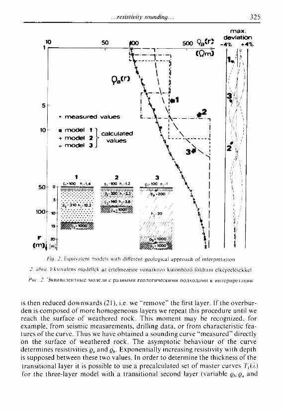
It is obvious from the preceding part that there is no problem in calculating the resistivity sounding curve for sections with homogeneous and transitional layers. In contrast, it is not so easy to interpret the measured field curve. The first important step in the interpretation procedure is to introduce the geological model. In our case the model has three main parts: surface layer of homoge­neous resistivity (or layers), weathered rock (transitional layer) and un­weathered rock with constant resistivity. The necessity for this geological- geophysical approach is illustrated in Fig. 2. The measured curve may be interpreted (within given limits of accuracy) in terms of at least three equivalent models with different geological meanings. If we suppose the existence of weathered rock, then model 3 is most acceptable. We use this model to interpret similar sounding curves in the given area.

At present, many interpretation techniques exist. One of them is the inter­pretation in the resistivity transform domain, which utilizes recursive relation for the succesive “removal" of upper layers [K o efo ed 1979b]. This method is particularly important in our case because it enables us to reduce the measured curve on the surface of the transitional. A combined graphical and numerical method of interpretation has been elaborated consisting of the following.

The measured curve gjr) is first transformed into curve Tj(A) by means of relation (25). The resistivity and thickness of the first layer are determined graphically by two-layer master curves (in the ga(r) or 7](A) domain). The curve

. . .resistivity sounding... 325

Ю 50 (Ю0----------------------, -------------------------

9 a « r > \ \

r V - V

• m e a s u r e d v a lu e s V - '

10 ■ m o d e l 1 m o d e l 2 m o d e l 3

_ c a lc u la te d * m o d e l 2 ■ v a |u e s>\

m a x .^ / м d e v ia tio n

500 V a 'r ' - 4 % + 4 %иb l\I \

COm)

\ --------\

\V '-- -3 ^ 4

о

4

s

50

100

r(m)j

9 ,-Ю 0 h,=1.4

5

Ю

15-f

20M

-.ç2 = 310 h,=12.2

291-Ю 0 h1=1.2

•.••.92r3j20:h3r2r3;.

vT 4v,V(V(A

3100 h.=1

щлшштт/ 9a *200 \h,= 20

\ !

v

ji /3 'irI .1\/\

Ä;l \

/ / j

;/ \'J I

/•'«/. 2, Equivalent models with different geological approach of interpretation

2. ábra. Ekvivalens modellek az értelmezésre vonatkozó különböző földtani elképzelésekkel

Puc. 2. Эквивалентные модели с разными геологическими подходами к интерпретации

is then reduced downwards (21), i.e. we “remove” the first layer. If the overbur­den is composed of more homogeneous layers we repeat this procedure until we reach the surface of weathered rock. This moment may be recognized, for example, from seismic measurements, drilling data, or from characteristic fea­tures of the curve. Thus we have obtained a sounding curve “measured” directly on the surface of weathered rock. The asymptotic behaviour of the curve determines resistivities ga and gb. Exponentially increasing resistivity with depth is supposed between these two values. In order to determine the thickness of the transitional layer it is possible to use a precalculated set of master curves T,(/) for the three-layer model with a transitional second layer (variable gh/ga and

326 L. Zima

constant h2lh\). There may be several such sets for suitable ratios h2lhx and on comparing the reduced curve with these we obtain h2.

Another method for the approximate determination of the thickness of the transitional layer uses longitudinal conductance S. The decrease in conductance Sg with depth in the transitional layer may be expressed as

dSg = ~ (26)Q(z)

After substituting relation (5) for g(z) and in consequence of (6), integrating (26) from dj_ , to d{ gives

^ _ hi Qb Qa9 QaQb , Qb (27)In —

QaThe resistivities ga, gh are known and Sg may be determined by subtracting the longitudinal conductances = h1/g1, S2 = h2/Q2, ••• from the total conduc­tance 5. The total conductance can be defined graphically by means of two-layer master curves [K eller and F r is c h k n e c h t 1970, M atveev 1974]. Thus

In *ht = QaQb— ^ [ S - ( S t + S2 + . . . ) ] , - S '

Qb QaThe final step is to calculate the sounding curve (Т^Д) or ga(r)) for inter­

preted parameters of the whole section, comparing the calculated curve with the measured curve. Interpretation is complete when the calculated and measured curves coincide. If there is some discrepancy, interpretation should be repeated after modifying the resistivities and thicknesses.

4. Practical examples

Some results obtained from interpreting sounding curves from metamor- phic rock area in SE Bohemia are presented. Biotite paragneiss is the dominat­ing rock in this area; it is mostly covered with unconsolidated sediments (sand, gravel, clay) of small thickness. Fractured zones and deeply weathered parts of gneiss are suitable places for migration and accumulation of ground water. Resistivity sounding (Schlumberger array) in combination with shallow refrac­tion seismics were used for determining depth and intensity of weathering and the VLF method was used for searching for linear zones of fractured rocks.

An example of the interpretation of a resistivity sounding curve near a well is shown in Fig. 3. Sands and gravel-sands with resistivity of 460 Dm are deposited under the surface soil. The upper part of the bedrock consists of quite decomposed weathered gneiss (sand-clay eluvium) which has a resistivity of

. . .resistivity sounding... 327

Fig. 3. Example of interpretation of resistivity sounding curve near a well and comparison withresistivity log

3. úbru. Példa fúrólyuk közelében nyert ellenállás-szondázási görbe kiértékelésére és az eredmény összehasonlítása a lyukban felvett ellenállás-szelvénnyel

Puc. 3. Пример интерпретации кривой зондирования по методу сопротивления вблизи скважины и ее сопоставление с каротажной диаграммой сопротивления

about 250 Qm. Successive transition through strongly jointed weathered parts into slightly jointed and compact gneiss appears lower. It is characterized by increasing resistivity with depth. The interpretation of weathered rock as a transitional layer corresponds well with the resistivity log curve.

It is known that in weathered rock the seismic velocity is lower than in compact rock. Thus the weathered rock zone may be regarded as a velocity transitional layer too [D o r tm a n 1976]. This problem was studied by S k o pec and H r á c h [1976]. They elaborated a special interpretation procedure for determining the distribution of velocities of seismic waves at various depths. Figure 4 demonstrates a comparison of their results with the interpretation of resistivity sounding measurements. The unconsolidated overburden with a thickness of 2.4 m has a velocity of 300 m/s and a resistivity of 330 Qm. Strongly weathered gneiss has a surface velocity of 1400 m/s and a resistivity of 460 Qm. In the downgoing direction both resistivity and seismic velocity increase. Even at depths of 5-7 m gneiss may still be considered as weathered rock (2000 m/s, 500-600 Qm).

328 L. Zima

• measured » calculated values

Fig. 4. The results of interpretation of resistivity and seismic measurements

4. ábra. Az ellenállásmérések cs a szeizmikus mérések kiértékelésének eredménye

Puc. 4. Результаты интерпретации кривых сопротивления и данных сейсморазведки

Joint interpretation of resistivity and seismic measurements was carried out at many places in the given area. Comparison of interpreted resistivities and seismic velocities in weathered gneiss with respect to drilling results is sum­marized in Fig. 5. This figure enables one to approximate by estimate the weathering intensity on the basis of resistivities and seismic velocities.

In the lower part of Fig. 6 an interpretation of resistivity sounding measure­ments along profile A-A' is shown. High resistivities at small depth were found at sounding points Nos. 9-13. From Fig. 5 we may deduce the occurrence of compact or only slightly jointed gneiss under the overburden.

Another situation is at soundings Nos. 7 and 8 in the western part of the profile. Low resistivities on the surface of gneiss and relatively slow increase in their values with depth offers evidence of the presence of strongly weathered gneiss. The conductivity anomaly of the VLF method is also situated in this part of the profile (see upper part of Fig. 6). The anomalous VLF zone can be followed on several profiles and it is caused by fractured and weathered gneiss. It is also obvious that the ground-water well situated in this zone has five times higher specific yield than the other well localized outside this zone.

. . .resistivity sounding... 329

9 (Qm )100 500 1000 5000

1

2Ж

__ _

— я— 4

r̂rrm 5■ i i i _1_till i i i —1 i ill.■___ l L 1_I—t i l l - - ..J------1--- Í-- 1--1—1

Ю 0 500 1000 5000¥ Cm/s)

Fig. 5. Approximate estimation of gneiss weathering on the basis of resistivities and velocities 1 - decomposed gneiss (sand-clay eluvium); 2 weathered gneiss; 3 — slightly weathered,

strongly jointed gneiss; 4 slightly jointed gneiss; 5 compact gneiss

5. ábra. A gneisz mállottságának becslése, fajlagos ellenállások és sebességek alapján:1 — teljesen bontott gneisz (homokos-agyagos eluvium); 2 mállott gneisz; 3 gyengén

mállott. erősen repedezett gneisz; 4 gyengén repedezett gneisz; 5 — tömör gneisz

Puc. 5. Приблизительная оценка выветривания гнейсов на основании сопротивленийи скоростей

I совершенно разложенные гнейсы (песчано-глинистый элювий); 2 — выветрелые гнейсы: 3 - слабо выветрелые, сильно трещиноватые гнейсы; 4 слабо трещиноватые

гнейсы; 5 массивные гнейсы

5. Conclusions

A simple recursive formula for computing the resistivity transform function has been developed for transitional layers with exponential increase in resistivity with depth. A graphical-numerical method for interpreting resistivity soundig curves has been suggested. The method is based on interpreting the resistivity transform domain which opens the way to reducing the resistivity transform curve towards the surface of weathered rock. As has been demonstrated by practical examples, the assumption that the weathered rock may be approxi­mated by a transitional layer corresponds better to reality.

330 L. Z ima

A6I

7I

8I

9 10I I

A111 12 13I I I

620

Fig. 6. Results of resistivity sounding (lower part) and VLF measurements (upper part) at Pojbuky locality. North is at the top of the map

6. ábra. Az ellenállás-szondázások (alul) és VLF mérések (felül) eredménye Pojbuky közelében.A térkép E-felé van tájolva

Puc. 6. Результаты зондирований методом сопротивления (внизу) и измерений методом СДВР (вверху) — участок Пойбуки. Север — вверх по карте

. . .resistivity sounding... 331

REFERENCES

Banerjee B., Sengupta B. J. and Pal B P. 1980a: Apparent resistivity of a multilayered earth with a layer having exponcntiality varying conductivity. Geophysical Prospecting 28, 3, pp. 435-452

Banerjee B., Sengupta B. J. and Pal B. P. 1980b: Resistivity sounding on a multilayered earth containing transition layers. Geophysical Prospecting 28, 5, pp. 750-758

Dortman N. B. 1976: Physical Properties of Rocks (in Russian). Nedra, Moscow G hosh D. P. 1971a: The application of linear filler theory to the direct interpretation of geoelectrical

resistivity sounding measurements. Geophysical Prospecting 19, 2, pp. 192-217 G hosh D. P. 1971b: Inverse filter coefficients for the computation of apparent resistivity standard

curves for a horizontally stratified earth. Geophysical Prospecting 19, 4, pp. 769-775 G rant F. S. and West G. F. 1965: Interpretation Theory in Applied Geophysics. McGraw-Hill

Book Co., New York. 583 p.Jain S. C. 1972: Resistivity sounding on a three-layer transitional model. Geophysical Prospecting

20, 2, pp. 283-292Keller G. V. and Frischknecht F. C. 1970: Electrical Methods in Geophysical Prospecting.

Pergamon. Oxford, 519 p.Koefohd O. 1979a: Resistivity sounding on an earth model containing transition layers with linear

change of resistivity with depth. Geophysical Prospecting 27, 4, pp. 862-868 Koffoed O. 1979b: Geosounding Principles, I. Resistivity Sounding Measurements. Elsevier,

Amsterdam, 276 p.L a i . T. 1970: Apparent resistivity over a three-layer earth with an inhomogeneous interstratum. Pure

and Applied Geophysics 82, pp. 259-269M alitok К. and Roy A. 1968: Resistivity sounding on a two-layer earth with transitional boun­

dary. Geophysical Prospecting 16, 4, pp. 436-446 Mallick K. and Jain S. 1979: Resistivity sounding on a layered transitional earth. Geophysical

Prospecting 27, 4. pp. 869-875Matvef.v B. K. 1974: Interpretation of Electromagnetic Soundings (in Russian). Nedra, Moscow Mundry E. and Zschau H.-J. 1983: Gcoelectrical models involving layers with a linear change in

resistivity and their use in the investigation of clay deposits. Geophysical Prospecting 31, 5.pp. 810-828

N yman D. C. and Landisman M. 1977: VES dipole-dipole filter coefficients. Geophysics 42, 5. pp. 1037-1044

Ollier C. 1969: Weathering. EdinburghPatella D. 1977: Resistivity sounding on a multi-layered earth with transitional layers. Part 1:

Theory. Geophysical Prospecting 25, 4, pp. 699-729 Patella D. 1978: Resistivity sounding on a multi-layered earth with transitional layers. Part II:

Theoretical and field examples. Geophysical Prospecting 26, 1, pp. 130-156 Paul M. K. and Banerjee B. 1970: Electrical potentials due to a point source upon models of

continuously varying conductivity. Pure and Applied Geophysics 80, pp. 218-237 Skopec J. and H rách S. 1976: Interpretation of a medium with vertical velocity gradient by means

of difference curves (in Czech). Acta Universitatis Carolinae, Geologica 4, pp. 295-308 Slighter L. B. 1933: The interpretation of the resistivity prospecting method for horizontal

structures. Physics 4, pp. 307-322Stötzner U. 1975: fngenieurgeophysikalische Untersuchungsmethodik und Komplexinterpreta­

tion zur Lösung felsmechanischer Aufgaben. Freiberger Forschungshefle C-307, Leipzig, 114 p.

Stoyer C. H. and W ait J. R. 1977: Resistivity probing of an “exponential’’ earth with a homoge­neous overburden. Geoexploration 15, 1, pp. 11-18

Sunde E. D. 1949: Earth Conduction Effects in Transmission Systems. D. Van Nostrand Co., New York

332 / , . Zima

MÁLLÓIT KŐZETEKEN VÉGZETT ELLENÁLLÁS-SZONDÁZÁS KIÉRTÉKELÉSE

L. ZIMA

A mélységgel exponenciálisan növekvő ellenállásról feltételezzük, hogy az mállóit kőzeteken álló (átmeneti) réteget jelez. Erre az esetre egy egyszerű rekurzív képletet vezettünk le. a fajlagos ellenállás transzformációs függvényének kiszámításához. Ez a függvény könnyen kiszámítható változó es állandó ellenállású rétegeket tartalmazó szelvényre, a tárgyalt képlet és az állandó fajlagos ellenállású rétegekre kidolgozott, ismert rekurzív képlet összekapcsolása útján. Az ellenállás-szon- dázási görbe megkapható az ellenállás transzformációs függvény és szürőegyütthatók digitális konvoluciójával. A terepi görbék kiértékelése nehéz és egy feltételezett fajlagos ellenallás-modellen kell alapulnia. A kiértékeléshez numerikus és grafikus módszerek kombinációját javasoljuk, a fajlagos ellenállás transzformációs tartományában. Kiértékelési példát mutatunk be metamorf kőzetek területéről. Ismertetjük az eredményeket és összehasonlítjuk ezeket a fúrási és szeizmikus adatokkal.

ИНТЕРПРЕТАЦИЯ КРИВЫХ ЗОНДИРОВАНИЯ МЕТОДОМ СОПРОТИВЛЕНИЯВ ВЫВЕТРЕЛЫХ ПОРОДАХ

Л. ЗИМА

Сопротивление, возрастающее с глубиной по экепоненцияльному закону, предположи­тельно является признаком наличия (переходной) зоны выветрелых пород. Для этого случая была разработана простая рекурсивная формула с целью вычисления функции преобразова­ния сопротивления. Функция преобразования сопротивления может быть легко вычислена для разрезов, состоящих их переходных слоев и слоев постоянного удельного сопротивле­ния. путем сочетания обсуждаемой формулы с известной рекурсивной формулой для слоев постоянного удельного сопротивления. Кривая зондирования по методу сопротивления может быть получена пу гем цифровой конволюции функции преобразования сопротивления и фильтровых коэффициентов. Интерпретация полевых кривых трудоемка и должна базиро­ваться на предполагаемой модели разреза удельных сопротивлений. Рекомендуется комби­нация цифровых и графических методов в области преобразования сопротивлений для ин- 1 ерпретации. Приводятся примеры интерпретации из района распространения метаморфи­ческих пород. Полученные результаты обсуждаются и сопоставляются с данными бурения и сейсморазведки.