2d electrical resistivity tomography …journals.bg.agh.edu.pl/geology/2013.39.4/geol.2013.39.4...2d...

331

http://dx.doi.org/10.7494/geol.2013.39.4.331

2d ElECTriCAl rESiSTiviTy TOmOgrAphy iNTErprETATiON AmBiguiTy –

ExAmplE Of fiEld STudiES SuppOrTEd wiTh ANAlOguE ANd NumEriCAl mOdElliNg

grzegorz BANiA & michał ĆwiKliK

AGH University of Science and Technology, Faculty of Geology, Geophysics and Environmental Protection, Department of Geophysics;

al. Mickiewicza 30, 30-059 Krakow, Poland; e-mail: [email protected], [email protected]

Abstract: Single Electrical Resistivity Tomography (ERT) survey was carried out in the Manor and Park Complex in Nowa Huta (Krakow Branice, Poland). It was applied at a small distance and pa-rallel to the longer wall of a monumental building containing an empty 3 m deep basement. Analogue modelling was performed in order to recreate the field study at the proper scale. The laboratory set-up consisted of a water tank where electrodes were mounted to the particular plate, which rested on wa-ter surface. The basement model was made out of a non-conducting material. The default and robust inversions were tested and these variants were also considered with the use of numerical modelling. Laboratory experiments have confirmed that zones visible in the interpreted field section are caused by the influence of the building cellar located next to the survey line. Zones of this kind are additio-nally disturbed by the local geological structure. The experiment has pointed out, among others, that as the distance between the survey line and the underground body increases, the inversion results are still burdened by an object influence. Thus, similar situations can be verified with the use of analogue modelling presented in this paper or 3D numerical one.

Key words: Electrical Resistivity Tomography (ERT), ambiguity, 2D inversion, analogue and nume-rical modelling

Geology, Geophysics & Environment 2013 Vol. 39 No. 4 331–339

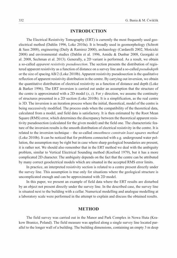
G. Bania & M. Ćwiklik332

iNTrOduCTiON

The Electrical Resistivity Tomography (ERT) is currently the most frequently used geo-electrical method (Dahlin 1996, Loke 2010a). It is broadly used in geomorphology (Schrott & Sass 2008), engineering (Daily & Ramirez 2000), archaeology (Cardarelli 2002, Mościcki 2008) and environmental studies (Dahlin et al. 1996, Amidu & Dunbar 2008, Georgaki et al. 2008, Sechman et al. 2013). Generally, a 2D variant is performed. As a result, we obtain a so-called apparent resistivity pseudosection. The section presents the distribution of regis-tered apparent resistivity as a function of distance on a survey line and a so-called pseudodepth or the size of spacing AB/2 (Loke 2010b). Apparent resistivity pseudosection is the qualitative reflection of apparent resistivity distribution in the centre. By carrying out inversion, we obtain the quantitative distribution of electrical resistivity as a function of distance and depth (Loke & Barker 1996). The ERT inversion is carried out under an assumption that the structure of the centre is approximated with a 2D model (x, z). For y direction, we assume the continuity of structures presented in a 2D section (Loke 2010b). It is a simplification, as the real centre is 3D. The inversion is an iteration process where the initial, theoretical, model of the centre is being successively modified. The process ends when the compatibility of the theoretical data, calculated from a model, and field data is satisfactory. It is then estimated by the Root Mean Square (RMS) error, which determines the discrepancy between the theoretical apparent resis-tivity pseudosection (calculated for the given model) and the field one. The characteristic fea-ture of the inversion results is the smooth distribution of electrical resistivity in the centre. It is related to the inversion technique – the so-called smoothness constrain least squares method (Loke 2010b). It can be noticed that for problems connected with e.g. underground water pol-lution, the assumption may be right but in case where sharp geological boundaries are present, it is rather not. We should also remember that in the ERT method we deal with the ambiguity problem, similar to Vertical Electrical Sounding method (Koefoed 1979), but it has a more complicated 2D character. The ambiguity depends on the fact that the centre can be attributed by many correct geoelectrical models which are situated in the accepted RMS error limits.

In practice, an interpreted resistivity section is related to a centre present directly under the survey line. This assumption is true only for situations where the geological structure is uncomplicated enough and can be approximated with 2D model.

In this paper, we present an example of field data where the ERT results are disturbed by an object not present directly under the survey line. In the described case, the survey line is situated next to the building with a cellar. Numerical modelling and analogue modelling at a laboratory scale were performed in the attempt to explain and discuss the obtained results.

mEThOd

The field survey was carried out in the Manor and Park Complex in Nowa Huta (Kra-kow Branice, Poland). The field measure was applied along a single survey line located par-allel to the longer wall of a building. The building dimensions, containing an empty 3 m deep

2D Electrical Resistivity Tomography interpretation... 333

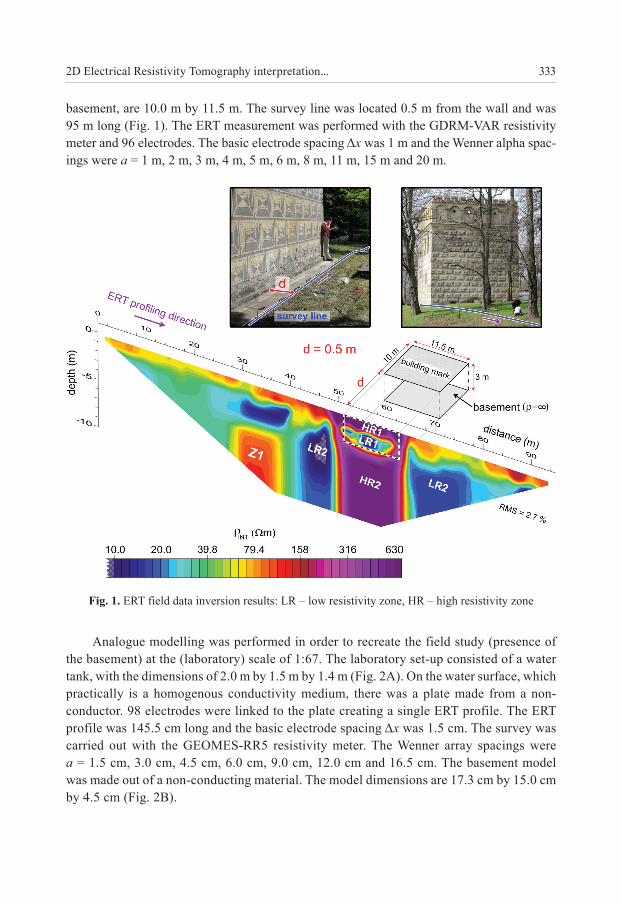
basement, are 10.0 m by 11.5 m. The survey line was located 0.5 m from the wall and was 95 m long (Fig. 1). The ERT measurement was performed with the GDRM-VAR resistivity meter and 96 electrodes. The basic electrode spacing Δx was 1 m and the Wenner alpha spac-ings were a = 1 m, 2 m, 3 m, 4 m, 5 m, 6 m, 8 m, 11 m, 15 m and 20 m.

fig. 1. ERT field data inversion results: LR – low resistivity zone, HR – high resistivity zone

Analogue modelling was performed in order to recreate the field study (presence of the basement) at the (laboratory) scale of 1:67. The laboratory set-up consisted of a water tank, with the dimensions of 2.0 m by 1.5 m by 1.4 m (Fig. 2A). On the water surface, which practically is a homogenous conductivity medium, there was a plate made from a non-conductor. 98 electrodes were linked to the plate creating a single ERT profile. The ERT profile was 145.5 cm long and the basic electrode spacing Δx was 1.5 cm. The survey was carried out with the GEOMES-RR5 resistivity meter. The Wenner array spacings were a = 1.5 cm, 3.0 cm, 4.5 cm, 6.0 cm, 9.0 cm, 12.0 cm and 16.5 cm. The basement model was made out of a non-conducting material. The model dimensions are 17.3 cm by 15.0 cm by 4.5 cm (Fig. 2B).


fig. 2. Laboratory settings (A) and analogue modelling inversion results (B): LR – low resistivity zone, HR – high resistivity zone

The laboratory measurements were conducted on four profiles. In the first case, the mod-el was moved 7.5 mm from the survey line. In the next cases, the distance was 15.0 mm, 22.5 mm and 30.0 mm. For the field surveys it is equivalent to: 0.5 m, 1.0 m, 1.5 m and 2.0 m. In the laboratory experiments some scaling problems related to limited dimensions of the wa-ter tank, electrodes size, etc. occurred. In order to limit the measurement errors, each ERT survey was conducted twice. At stage one, a measurement was carried out without the mod-el (N – uniform half space + noise). Afterwards, the survey was repeated with the model (A – anomaly + noise). All survey results were normalized. Apparent resistivity values for the anomaly were divided by corresponding apparent resistivity values for the noise (A/N). The normalization allowed distinguishing mainly the anomaly coming from the model.

The field and laboratory ERT data were inverted with RES2DINV software (Loke 2010a). Default settings, like e.g. mesh grid size, were used. The default and robust inver-sion (Loke et al. 2003) options were tested. These variants were also considered with the use of numerical modelling which was performed with RES2DMOD software (Loke 2002). For this, four geometrical models were made (Fig. 3A). They were characterised by sharp

A B


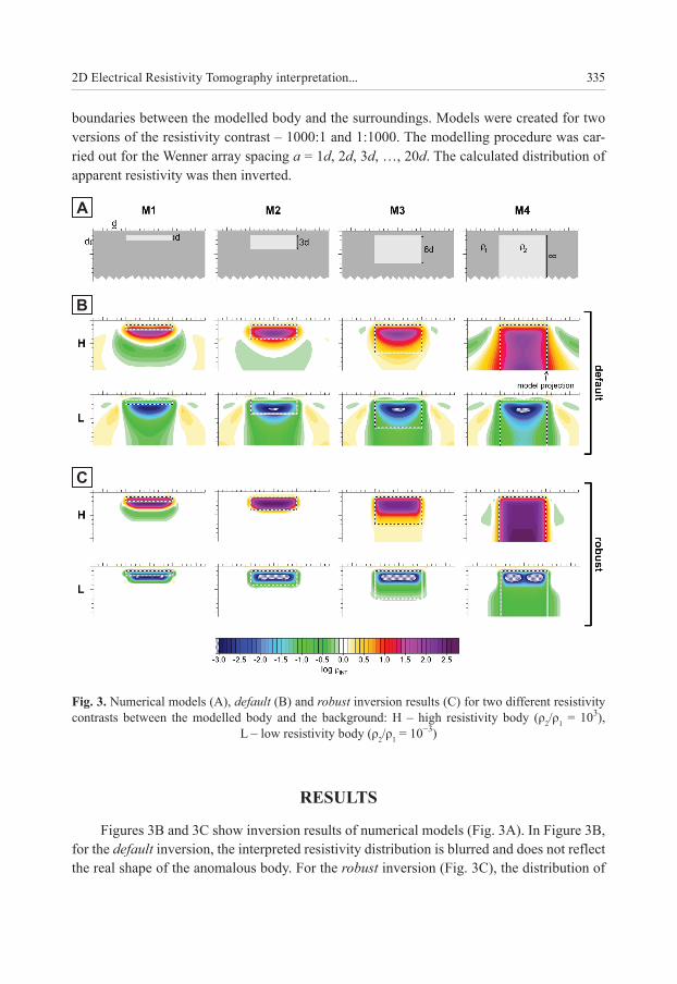
boundaries between the modelled body and the surroundings. Models were created for two versions of the resistivity contrast – 1000:1 and 1:1000. The modelling procedure was car-ried out for the Wenner array spacing a = 1d, 2d, 3d, …, 20d. The calculated distribution of apparent resistivity was then inverted.

fig. 3. Numerical models (A), default (B) and robust inversion results (C) for two different resistivity contrasts between the modelled body and the background: H – high resistivity body (ρ2/ρ1 = 103),

L – low resistivity body (ρ2/ρ1 = 10−3)

rESulTS

Figures 3B and 3C show inversion results of numerical models (Fig. 3A). In Figure 3B, for the default inversion, the interpreted resistivity distribution is blurred and does not reflect the real shape of the anomalous body. For the robust inversion (Fig. 3C), the distribution of

A

B

C


the isolines is closer to the real object shape than in the previous case. Inversion results show, apart from the real objects (models) mapping, false anomalies as well. These anomalies are often beyond the model boundaries. Anomalies for the default variant are clearly larger than for the robust variant.

Object mapping differs for different interpretation variants. It depends on the geometri-cal situation. The object mapping is the most precise for the M2 model (Fig. 3B, C). Inversion results for the M1 model show that the anomaly is slightly deeper than the modelled body. In the M3 case, the anomaly concentrates in the upper half of the assumed object. In inversion results for the M4 model, we can observe a clear difference for opposite resistivity contrasts. For good conductive objects (L), there are considerably lower interpreted resistivity zones than the resistivity of the assumed object. This can be explained by the complicated character of the current flow for such geometrical configuration.

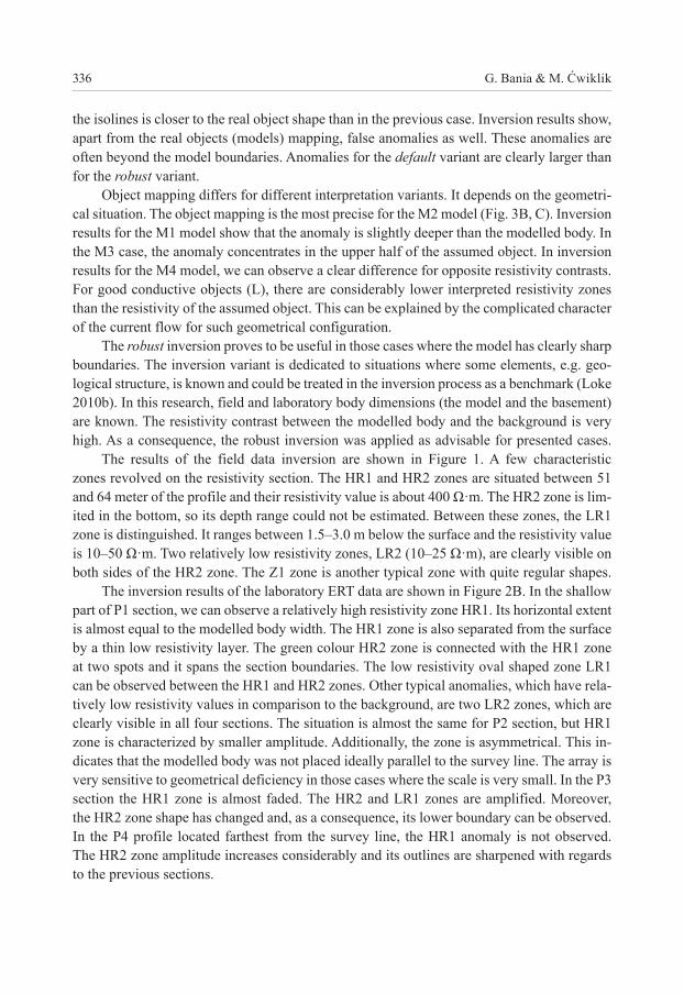
The robust inversion proves to be useful in those cases where the model has clearly sharp boundaries. The inversion variant is dedicated to situations where some elements, e.g. geo-logical structure, is known and could be treated in the inversion process as a benchmark (Loke 2010b). In this research, field and laboratory body dimensions (the model and the basement) are known. The resistivity contrast between the modelled body and the background is very high. As a consequence, the robust inversion was applied as advisable for presented cases.

The results of the field data inversion are shown in Figure 1. A few characteristic zones revolved on the resistivity section. The HR1 and HR2 zones are situated between 51 and 64 meter of the profile and their resistivity value is about 400 Ω·m. The HR2 zone is lim-ited in the bottom, so its depth range could not be estimated. Between these zones, the LR1 zone is distinguished. It ranges between 1.5–3.0 m below the surface and the resistivity value is 10–50 Ω·m. Two relatively low resistivity zones, LR2 (10–25 Ω·m), are clearly visible on both sides of the HR2 zone. The Z1 zone is another typical zone with quite regular shapes.

The inversion results of the laboratory ERT data are shown in Figure 2B. In the shallow part of P1 section, we can observe a relatively high resistivity zone HR1. Its horizontal extent is almost equal to the modelled body width. The HR1 zone is also separated from the surface by a thin low resistivity layer. The green colour HR2 zone is connected with the HR1 zone at two spots and it spans the section boundaries. The low resistivity oval shaped zone LR1 can be observed between the HR1 and HR2 zones. Other typical anomalies, which have rela-tively low resistivity values in comparison to the background, are two LR2 zones, which are clearly visible in all four sections. The situation is almost the same for P2 section, but HR1 zone is characterized by smaller amplitude. Additionally, the zone is asymmetrical. This in-dicates that the modelled body was not placed ideally parallel to the survey line. The array is very sensitive to geometrical deficiency in those cases where the scale is very small. In the P3 section the HR1 zone is almost faded. The HR2 and LR1 zones are amplified. Moreover, the HR2 zone shape has changed and, as a consequence, its lower boundary can be observed. In the P4 profile located farthest from the survey line, the HR1 anomaly is not observed. The HR2 zone amplitude increases considerably and its outlines are sharpened with regards to the previous sections.


diSCuSSiON

Analogue modelling inversion results (Fig. 2B) show a considerable similar-ity to the field data inversion results (Fig. 1). The field survey line should be compared to the laboratory P1 profile as it corresponds to the field data situation in the appropriate scale. The interpreted HR1, HR2 and LR1 zones in P1 section (Fig. 2B) have similar distri-bution and shapes like HR1, HR2 and LR1 zones in the field section (Fig. 1). We can also observe that in both sections LR2 zones are visible. In laboratory sections they are placed a little deeper. The zones of this kind are often observed in the inversion results in a situ-ation where the centre has a regularly-shaped body with a much higher resistivity than resistivity of the background. Similar effects can be observed in ERT inversion sections from the Krakow Main Square Market, where the water tank from World War II was found (Mościcki 2008). It should be noted that HR2 zone in the field section (Fig. 1) has practi-cally the same shape and it is not limited at the base as the object interpreted from numeri-cal modelling (Fig. 3C – M4, H). However, we do not observe analogical LR2 zones next to the object. The appearance of such zones would require additional explanation.

The analysis of the laboratory results (Fig. 2B) shows that as the distance between sur-vey line and model increases, all distinguished zones (expect of LR2) change their amplitudes and shapes or even vanish (HR1). This results from the underground object being present in some distance from the survey line that has difficult to evaluate influence on the survey results. Therefore, the 2D section, obtained as a result of ERT surveys, cannot be unambigu-ously treated as information that comes directly from below the survey line. It is because we are also dealing with the influence of the survey line surroundings. Cardarelli & Di Filippo (2009) reported similar observations. As a result, there are some interpreted zones, which are not present in reality under the survey lines in every analysed section.

The Z1 zone in field section (Fig. 1), with the resistivity value of ca. 70 Ω·m, has a regular shape. It should be noted that this zone should not be treated as an interpreted effect from a regular rectangular object. Its appearance can be a side effect of applying the robust inversion (Loke et al. 2003). This option resulted in sharp edges; also, this fragment was attributed the shape of a regular geometric block. We observe similar effects in interpreted sections showing the presence of cavities in the eastern part of Saudi Arabia as discussed by Metwaly & AlFouzan (2013).

CONCluSiONS

Laboratory experiments (Fig. 2) confirmed that interpreted zones visible in field section (Fig. 1) are caused by the influence of the building cellar being placed next to the survey line. It should be noted that zones of this kind are additionally disturbed by the local geological structure. The experiment pointed out that as the distance between the survey line and the un-derground body increases, the inversion results are still suffering from object influence. In all


laboratory cases, there were no physical objects under ERT survey lines shapes and distribu-tion of which could correspond to those visible in the interpreted sections.

Authors also turned their attention to the problem connected with zones such as LR2 which are visible in inversion results (Figs 1, 2B). They occur in field data and analogue modelling results when some contrasting (with background) underground body is present under or next to the survey line. We do not observe these zones in numerical modelling re-sults. The 2D ERT surveys results are carried out by 2D inversion, which simplifies the 3D structure of the centre with the use of 2D section. In practice, the interpreted image is treated as everything that is located directly under the survey line. This assumption is true only for the situation where the geological structure is not complicated enough and can be estimated as 2D model. In reality, such situation can be found very rarely.

While conducting ERT surveys, the data is influenced by many objects located at some distance from the survey line. Therefore, e.g. when surveys are being made on limited area and next to buildings or walls, we should take care about influence of such objects on the ob-tained results. Situations of this kind can be verified with the use of analogue modelling (presented in the article) or 3D numerical one.

Authors are grateful to dr. Włodzimierz Jerzy Mościcki for help and advice.

The work was financially supported by Dean’s Grants no. 15.11.140.334 and no. 15.11.140.335.

rEfErENCES

Amidu S.A. & Dunbar J.A., 2008. An evaluation of the electrical-resistivity method for wa-ter-reservoir salinity studies. Geophysics, 73, 4, G39–G49.

Cardarelli E., 2002. Geoelectric survey by ERT to investigate marble ruins at the Roman forum, Rome, Italy. European Journal of Environmental and Engineering Geophysics, 7, 219–228.

Cardarelli E. & Di Filippo G., 2009. Integrated geophysical methods for the characterisation of an archaeological site (Massenzio Basilica – Roman forum, Rome, Italy). Journal of Applied Geophysics, 68, 508–521.

Dahlin L.T., 1996. 2D resistivity surveying for environmental and engineering applications. First Break, 14, 7, 275–283.

Dahlin L.T., Forsberg K., Nilsson A. & Flyhammer P., 2006. Resistivity Imaging for Map-ping of Groundwater Contamination at the Municipal Landfill La Chureca, Managua, Nicaragua. Near Surface 2006, 12th European Meeting of Environmental and Engineer-ing Geophysics, 4–6 September, Helsinki, Finland.

Daily W. & Ramirez A.L., 2000. Electrical imaging of engineered hydraulic barriers. Geo-physics, 65, 1, 83–94.


Georgaki I., Soupios P., Sakkas N., Ververidisa F., Trantasa E., Vallianatos F. & Manios T., 2008. Evaluating the use of electrical resistivity imaging technique for improving CH4 and CO2 emission rate estimations in landfills. Science of the Total Environment, 389, 522–531.

Koefoed O., 1979. Geosounding Principles. Elsevier, Amsterdam.Loke M.H., 2002. RES2DMOD ver. 3.01. Rapid 2D resistivity forward modelling using

the finite-difference and finite-elements method. Geotomo Software. Manual.Loke M.H., 2010a. RES2DINV ver. 3.59 for Windows XP/Vista/7, Rapid 2-D Resistivity & IP

inversion using the least-squares method. Geotomo Software. Manual.Loke M.H., 2010b. Tutorial: 2-D and 3-D electrical imaging surveys. Geotomo Software.Loke M.H. & Barker R.D., 1996. Least squares deconvolution of apparent resistivity pseudo-

sections. Geophysics, 60, 6, 1682–1690.Loke M.H., Ackworth I. & Dahlin T., 2003. A comparison of smooth and blocky inversionmethods in 2D electrical imaging surveys. Exploration Geophysics, 34, 182–187.Metwaly M. & AlFouzan F., 2013. Application of 2-D geoelectrical resistivity tomography

for subsurface cavity detection in the eastern part of Saudi Arabia. Geoscience Fron-tiers, 4, 4, 469–476.

Mościcki W.J., 2008. The application of resistivity investigations in archaeology – two case studies from Krakow, Poland. Near Surface 2008, 14th European Meeting of Environ-mental and Engineering Geophysics, 15–17 September 2008 Krakow, Poland. Extended Abstracts & Exhibitors’ Catalogue, P58.

Schrott L. & Sass O., 2008. Application of field geophysics in geomorphology: Advances and limitations exemplified by case studies. Geomorphology, 93, 55–73.

Sechman H., Mościcki W.J. & Dzieniewicz M., 2013. Pollution of near-surface zone in the vi-cinity of gas wells. Geoderma, 197–198, 193–204.

2d electrical resistivity tomography …journals.bg.agh.edu.pl/geology/2013.39.4/geol.2013.39.4...2d...

Documents