cross-hole resistivity tomography using different electrode configurations
DESCRIPTION
Geophysical Prospecting, 2000, 48, 887±912Cross-hole resistivity tomography using differentelectrode configurationsZhou Bing1 and S.A. GreenhalghTRANSCRIPT

Geophysical Prospecting, 2000, 48, 887±912
Cross-hole resistivity tomography using differentelectrode configurations
Zhou Bing1 and S.A. Greenhalgh2
Abstract
This paper investigates the relative merits and effectiveness of cross-hole resistivitytomography using different electrode configurations for four popular electrode arrays:
pole±pole, pole±bipole, bipole±pole and bipole±bipole. By examination of two
synthetic models (a dipping conductive strip and a dislocated fault), it is shown thatbesides the popular pole±pole array, some specified three- and four-electrode
configurations, such as pole±bipole AM±N, bipole±pole AM±B and bipole±bipole
AM±BN with their multispacing cross-hole profiling and scanning surveys, are usefulfor cross-hole resistivity tomography. These configurations, compared with the pole±
pole array, may reduce or eliminate the effect of remote electrodes (systematic error)
and yield satisfactory images with 20% noise-contaminated data. It is also shown thatthe configurations which have either both current electrodes or both potential
electrodes in the same borehole, i.e. pole±bipole A±MN, bipole±pole AB±M and
bipole±bipole AB±MN, have a singularity problem in data acquisition, namely lowreadings of the potential or potential difference in cross-hole surveying, so that the
data are easily obscured by background noise and yield images inferior to those from
other configurations.
Introduction
Direct current (DC) electric surveying (sounding and profiling) along the earth'ssurface is a well-known geophysical exploration technique. Due to its conceptual
simplicity, low equipment cost and ease of use, the method is widely applied in mining
exploration, archaeological detection, civil and hydrological engineering, andenvironmental investigations. In traditional DC electrical resistivity surveying various
current±potential electrode arrangements, such as pole±pole, pole±bipole, bipole±
pole and bipole±bipole (dipole±dipole) arrays, are used, depending on theprospecting aims and the surface situation (e.g. site access). With the greater
computer power made available in recent years, there has been increasing interest in
q 2000 European Association of Geoscientists & Engineers 887
Received April 1999, revision accepted March 2000.1 Department of Geotechnology, Institute of Technology, Lund University, Box 118, S-221 00 Lund,
Sweden.2 Department of Geology and Geophysics, The University of Adelaide, Adelaide SA 5005, Australia.

DC resistivity imaging based on geophysical inversion theory. A number of research
articles have appeared on 2D and 3D DC resistivity imaging using surface scanning
pole±pole and bipole±bipole data (Smith and Vozoff 1984; Park and Van 1991; Liand Oldenburg 1992; Dabas, Tabbagh and Tabbagh 1994; Ellis and Oldenburg
1994b; Sasaki 1994; Zhang, Mackie and Madden 1995; Loke and Barker 1995,
1996). Xu and Noel (1993) discussed some independent measurements of surfaceelectrical surveys using two-, three- and four-electrode configurations for 2D or 3D
resistivity imaging.
Cross-hole DC electrical surveying, in which the source electrode (current injectionpoint) and the potential electrode (measuring point) are placed downhole in two
horizontally separated boreholes and moved over a range of depths, is able to yield
detailed information on the variation of electrical conductivity between the boreholes(Daniels 1977; Daniels and Dyck 1984; Shima 1992). Such cross-hole measurements
permit the detection and delineation of geological conditions between various source
and receiver locations. They offer potential advantages for greatly improving theeffectiveness of a test boring program by locating the targets more accurately.
Furthermore, the downhole electric measurements greatly extend the anomaly detection
capability beyond the performance limits of surface electric surveying. Owen (1983)discussed cross-hole bipole±bipole electric surveying to search for buried caves and
tunnels. Daniels and Dyck (1984) demonstrated a variety of applications of borehole
resistivity measurements to mineral exploration. Unfortunately, they did not intend toperform inversion with the data for cross-hole resistivity tomography.
In recent years, there has been growing interest in developing cross-hole DC
electrical surveying so as to image the 2D and 3D structure of the earth. Cross-holeresistivity imaging or tomography (Daily and Owen 1991; Shima 1992) is used to
reconstruct the conductivity structure of the earth using cross-hole scanning data.Most researchers have dealt with cross-hole resistivity tomography using pole±pole
array data (e.g. Daily and Owen 1991; Shima 1992), which is the simplest of all the
electrode arrays. In practical situations, the pole±pole array has two additional remoteelectrodes that have to be placed a long distance away from the working site (theory
assumes the current sink and the zero-voltage reference point to be at infinity, but in
practice, they never are). Obviously, it is not suitable to conduct such work in urbanareas or mine locations, because the data can easily be contaminated by noise from
other electric sources (e.g. power lines, leakage currents) along the wires connecting
the remote electrodes. According to Van, Park and Hamilton's (1991) fieldexperiment and Park and Van's (1991) result, it is not possible to collect data
accurately with a true pole±pole configuration in the field (about 15% of their data did
not satisfy reciprocity). The finite contribution of two remote electrodes introduces asystematic error into the inversion. Naturally, this prompts us to investigate other
electrode arrays for performing cross-hole electric surveys.
Possible ways to reduce this error may be either to decrease the number of remoteelectrodes or to re-deploy them in cross-hole data acquisition, e.g. applying either the
pole±bipole array to measure the potential difference between the two potential
888 Z. Bing and S.A. Greenhalgh
q 2000 European Association of Geoscientists & Engineers, Geophysical Prospecting, 48, 887±912

electrodes, the bipole±pole array to measure the potential with two opposite-polarity
current points (source and sink) or the bipole±bipole array to measure the potential
difference between two electrodes with two opposite-polarity current sources. If thesedata are available for cross-hole resistivity tomography, it not only reduces the effect of
remote electrodes, but also avoids the disturbance of random noise outside the
working site and makes it possible for the cross-hole resistivity tomography to beapplied to problems in civil engineering, groundwater studies and environmental
investigations within built-up areas. Zhou and Greenhalgh (1997) showed that there
are, respectively, six and three independent cross-hole configurations with pole±bipole/bipole±pole and bipole±bipole arrays. Furthermore, these arrays have better
target detection and delineation properties between two boreholes than the pole±pole
array, in the light of the sensitivity patterns and the anomaly effect. It is worthexploring the relative merits and effectiveness of cross-hole resistivity tomography
with such configurations. We use two synthetic models ± a dipping fracture and a
faulted bed ± to demonstrate the capabilities of cross-hole resistivity tomography withthese multipole configurations.
Theoretical methodology
DC resistivity modelling for cross-hole measurements reduces to solving the followingboundary-value problem for the 2.5D Green's function (Zhou 1998):
7´s7 G2:5D 2 k2
ysG
2:5D 2 dx 2 xcdz 2 zc ; x; z; xc; zc [ V;
2 G2:5D
2n1 B G
2:5D 0; x; z [ 2V;
8>><>>: 1
where s denotes conductivity, ky is the y-component of the 3D wavenumber,G
2:5Dx; ky; z is the ky-domain form of the 3D Green's function, n is the unit normal
vector for the boundary 2V enclosing V, the coordinate (xc,zc) is the location of a unit
current source and B is the boundary operator. The potential response to the current Iis easily obtained by multiplication:
U x; y; z I
2´F 2 1
c G2:5Dx; ky; z; 2
where F 2 1c denotes the inverse Fourier cosine transform with respect to the
wavenumber ky.
Applying Galerkin's scheme to (1) (Zienkiewicz 1971), we have the followingintegral equation for the 2.5D Green's function:X
i
V
s7Ni ´7Nj 1 k2ysNiNjdr 1
2V
sNjBNidG
G
2:5Di Njxc; zc;
j 1; 2; 3; :::;N: 3Here Ni (i 1,2,¼,N) is the ith shape function and G
2:5Di (i 1,2,¼,N) is the ith
Configurations for cross-hole resistivity tomography 889
q 2000 European Association of Geoscientists & Engineers, Geophysical Prospecting, 48, 887±912

nodal value of the Green's function. N is the total number of shape functions. After
dividing the range V and the boundary 2V into a set of subranges (elements) and
segments, e.g.
V X
e
Ve
and
2V X
e
Ge;
(3) reduces to the following linear equation system:
M G2:5D bc; 4
where
M MijN N ;Mij X
e
Aeij 1 Be
ij;
G2:5D G
2:5Di T; i 1; 2; :::;N;
bc Nixc; zcT; i 1; 2; :::;N; 5
and
Aeij
Ve
sx; z7Nix; z´7Njx; z 1 k2yNix; zNjx; zdV; 6
Beij
Ge
sx; zNix; zBNjx; zdG: 7
The matrix M is banded and positive-definite so that we can apply the banded
Cholesky decomposition (M LLT) to solve (4). This algorithm is very efficient forthe multiple-electrode measurements, because the decomposition is independent of
the vector bc, which relates to the position of the current electrodes (see (5)). After the
decomposition, the Green's functions G2:5Dxcj ; zcj ( j 1,2,..) for all the current
electrodes can be obtained efficiently by forward-substitution and back-substitution
due to the fact that the matrix L is a lower triangular matrix. Substituting the solution
for (2), the 3D electrical potential for arbitrary 2D media can be calculated.In resistivity field surveys, the quantity `apparent resistivity' rather than the
potential is used to indicate the variation in the electrical properties of the subsurface.
Apparent resistivity is defined by
ra KDU
I; 8
where DU UM 2 UN is the potential difference between the two potential electrodes
890 Z. Bing and S.A. Greenhalgh
q 2000 European Association of Geoscientists & Engineers, Geophysical Prospecting, 48, 887±912

and K is a geometric factor which depends on the electrode array configuration. The
subscripts M and N stand for the two potential electrodes (one of them may be
remote). In the following text, we use the italic letters A and B in the subscripts todenote the two current electrodes, one of which may also be remote. Considering the
fact that the Green's function G2:5Drj; rh vanishes when rj or rh is infinite (remote
electrode) and substituting (2) into (8), we can obtain a general form for the apparentresistivity for arbitrary array configurations:
ra K
2F 2 1
c d G2:5DMN rA 2 d G
2:5DMN rB; 9
where
d G2:5Djh r G
2:5Drj; r 2 G2:5Drh; r: 10
The above equations show that the apparent resistivities for different electrode arrays
can be calculated directly from the Green's functions.In order to perform resistivity inversion or tomography, we derived the explicit
expressions of the FreÂchet derivatives for apparent resistivity (Zhou and Greenhalgh
1995, 1999). For example, with the constant-point parametrizationser sedr 2 re, r [ Ve or the constant-block parametrization ser se,
r [ Ve, we obtained the following expressions:
2ra
2se 2
K
2F 2 1
c 7d G2:5DAB re´7d G
2:5DMN re 1 k2
ydG
2:5DAB red G
2:5DMN re; 11
or
2ra
2se 2
K
2F 2 1
c
Ve
7d G2:5DAB r ´7d G
2:5DMN r 1 k2
ydG
2:5DAB r d G
2:5DMN r dV
:
12Here Ve, located at re, represents a cell of the model whose conductivity is defined by a
constant se. Equations (11) and (12) can be computed for an arbitrary initial modeland therefore used to form the Jacobian matrix in an inversion procedure. Based on
the solution of (4) and expressions (9) and (11) or (12), we can apply an iterativeinversion algorithm, such as the generalized least-squares algorithm (Tarantola and
Vallette 1982), linearized algorithm (Pelton, Rijo and Swift 1978; Smith and Vozoff
1984; Tripp, Hohmann and Swift 1984; Dabas et al. 1994), the conjugate-gradientalgorithms (Ellis and Oldenburg 1994b), the smoothest model algorithms (Constable,
Parker and Constable 1987; Ellis and Oldenburg 1994a; Oldenburg and Li 1994;
LaBrecque et al. 1996) and the subspace algorithms (Skilling and Bryan 1984;Kennett and Williamson 1988; Oldenburg, McGillicray and Ellis 1993), to
reconstruct or image the resistivity structure between boreholes with the observed
data.
Configurations for cross-hole resistivity tomography 891
q 2000 European Association of Geoscientists & Engineers, Geophysical Prospecting, 48, 887±912
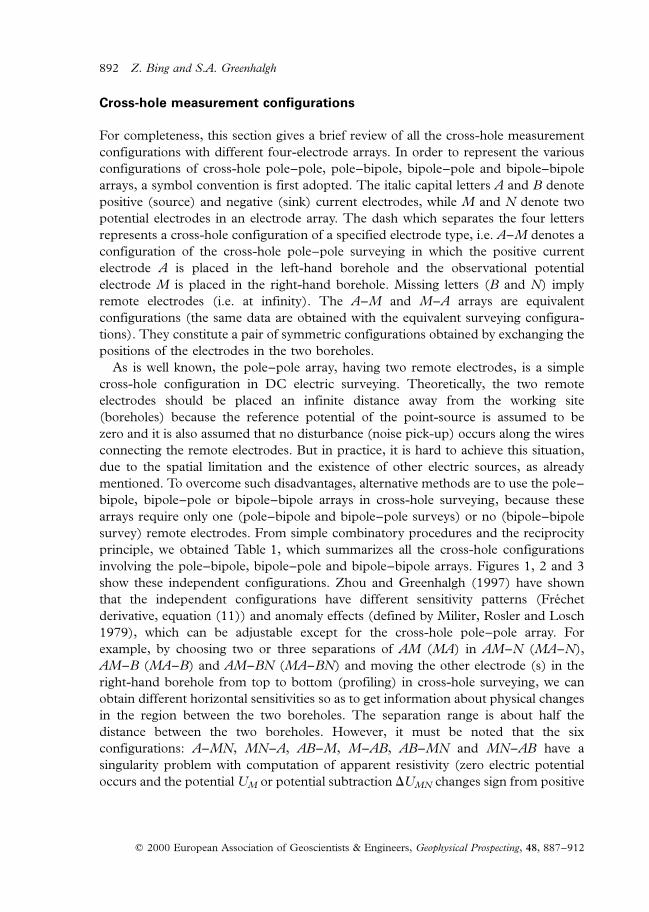
Cross-hole measurement configurations
For completeness, this section gives a brief review of all the cross-hole measurement
configurations with different four-electrode arrays. In order to represent the variousconfigurations of cross-hole pole±pole, pole±bipole, bipole±pole and bipole±bipole
arrays, a symbol convention is first adopted. The italic capital letters A and B denote
positive (source) and negative (sink) current electrodes, while M and N denote twopotential electrodes in an electrode array. The dash which separates the four letters
represents a cross-hole configuration of a specified electrode type, i.e. A±M denotes aconfiguration of the cross-hole pole±pole surveying in which the positive current
electrode A is placed in the left-hand borehole and the observational potential
electrode M is placed in the right-hand borehole. Missing letters (B and N) implyremote electrodes (i.e. at infinity). The A±M and M±A arrays are equivalent
configurations (the same data are obtained with the equivalent surveying configura-
tions). They constitute a pair of symmetric configurations obtained by exchanging thepositions of the electrodes in the two boreholes.
As is well known, the pole±pole array, having two remote electrodes, is a simple
cross-hole configuration in DC electric surveying. Theoretically, the two remoteelectrodes should be placed an infinite distance away from the working site
(boreholes) because the reference potential of the point-source is assumed to be
zero and it is also assumed that no disturbance (noise pick-up) occurs along the wiresconnecting the remote electrodes. But in practice, it is hard to achieve this situation,
due to the spatial limitation and the existence of other electric sources, as already
mentioned. To overcome such disadvantages, alternative methods are to use the pole±bipole, bipole±pole or bipole±bipole arrays in cross-hole surveying, because these
arrays require only one (pole±bipole and bipole±pole surveys) or no (bipole±bipole
survey) remote electrodes. From simple combinatory procedures and the reciprocityprinciple, we obtained Table 1, which summarizes all the cross-hole configurations
involving the pole±bipole, bipole±pole and bipole±bipole arrays. Figures 1, 2 and 3
show these independent configurations. Zhou and Greenhalgh (1997) have shownthat the independent configurations have different sensitivity patterns (FreÂchet
derivative, equation (11)) and anomaly effects (defined by Militer, Rosler and Losch
1979), which can be adjustable except for the cross-hole pole±pole array. Forexample, by choosing two or three separations of AM (MA) in AM±N (MA±N),
AM±B (MA±B) and AM±BN (MA±BN) and moving the other electrode (s) in the
right-hand borehole from top to bottom (profiling) in cross-hole surveying, we canobtain different horizontal sensitivities so as to get information about physical changes
in the region between the two boreholes. The separation range is about half the
distance between the two boreholes. However, it must be noted that the sixconfigurations: A±MN, MN±A, AB±M, M±AB, AB±MN and MN±AB have a
singularity problem with computation of apparent resistivity (zero electric potential
occurs and the potential UM or potential subtraction DUMN changes sign from positive
892 Z. Bing and S.A. Greenhalgh
q 2000 European Association of Geoscientists & Engineers, Geophysical Prospecting, 48, 887±912

Table 1. Cross-hole measurement configurations for different electrode arrays.
Electrode array Total no.No. of independentconfigurations Independent configurations ra singularity configurations
Pole±pole 2 1 A±MPole±bipole 12 6 AM±N, MA±N, MN±A, N±AM, N±MA, A±MN A±MN, MN±ABipole±pole 12 6 AM±B, MA±B, AB±M, B±AM, B±MA, M±AB AB±M, M±ABBipole±bipole 24 3 AM±BN, AM±NB, AB±MN AB±MN, MN±ABEquivalent array: Pole±bipole: AM±N, MA±N and MN±A Bipole±pole: MA±B, AM±B and AB±M
Con
figuration
sfor
cross-hole
resistivity
tomography
89
3
q2
00
0E
uro
pean
Asso
ciation
of
Geo
scientists
&E
ngin
eers,G
eophysicalP
rospecting,
48,
88
7±
91
2

to negative or negative to positive) in the profiling and scanning measurements. That
is, the geometric factor 1/K becomes zero.
Table 1 implies that if a certain number of electrodes are located in two boreholes,i.e. a total of 2n, then the maximum number of independent cross-hole pole±pole data
is n n n2 due to only one independent configuration, but the other arrays provide
more configurations for acquiring data about the variation in electrical resistivity ofthe medium. It is also shown that by employing the equivalent configurations between
the cross-hole pole±bipole and bipole±pole arrays (AM±N MA±B and MA±N AM±B) ± although the measurements are quite different (the former is used to
measure the potential difference of a source, the latter to measure the potential of a
pair of sources) ± inherently equivalent data can be obtained. Due to the singularityproblem, the configurations A±MN (M±AB) and AB±MN are not suitable for cross-
hole profiling measurements of apparent resistivity and it will be seen in the next
section that they are not as satisfactory as other configurations in cross-hole resistivitytomography. Consequently, besides the cross-hole pole±pole configuration A±M, six
other independent surveying configurations: AM±N, MA±N, AM±B, MA±B, AM±
BN and AM±NB are available for cross-hole profiling observations, and they may beemployed for cross-hole resistivity tomography.
Numerical imaging experiments
In the previous sections, it was shown that some specific cross-hole surveying
configurations involving pole±bipole, bipole±pole and bipole±bipole arrays can be
( A: current electrode, M , N: potential electrodes )
I V
I V
I V IV
IV IV
A
AA
A
A
A
M
M M
M
M M
N NN
N N
N
BB B
B
(a) (b) (c)
(d) (e) (f)
BB
∞
∞∞
∞
∞
Figure 1. Six independent configurations for cross-hole pole±bipole measurements: (a) AM±N,(b) MA±N, (c) MN±A, (d) N±AM, (e) N±MA and (f) A±MN. The capital letters A and B denotecurrent electrodes and M and N denote potential electrodes.
894 Z. Bing and S.A. Greenhalgh
q 2000 European Association of Geoscientists & Engineers, Geophysical Prospecting, 48, 887±912

adopted for cross-hole profiling measurements. To study the imaging capabilities with
these configurations, synthetic experiments were conducted for two models, Model-1and Model-2 (see Fig. 4). The first model comprises a dipping conductive strip
(resistivity 10 Vm) and the second model a dislocated fault (resistivity 10 Vm), each
embedded within a uniform background (resistivity 100 Vm). Each model isdiscretized into cells of dimensions 1 1 m2 (total 20 20 400 model para-
meters) and there are 21 electrodes evenly spaced at 1 m intervals in each of two
boreholes situated 10 m apart. The numerical experiments are individuallyimplemented with the independent cross-hole surveying configurations: pole±pole,
pole±bipole, bipole±pole and bipole±bipole arrays. For ease of comparison of the
imaging effectiveness with the different electrode arrays, the same inversion algorithm(conjugate-gradient method), the same initial model (uniform medium of
r 100 Vm) and the same constraints on the resistivities at the electrodes are usedin all the experiments. To avoid the singularity problem with apparent resistivity,
either the potential data UM or the potential difference data DUMN are used directly
for the inversions. The image reconstructions are accomplished using noise-free dataand noise-contaminated data. The noisy potential or potential difference is simulated
by DUnoise (1 1 b fnoise)DUsynthetic. Here fnoise is a random number between 21 and
11 and b 0.05, 0.1 and 0.2, corresponding to 5%, 10% and 20% noise levels. Tominimize the false information of the data for the image reconstructions, the inversion
algorithm automatically rejects portions of the data if they are of very poor quality, i.e.
the absolute value of the contaminated data is less than the root-mean-square (RMS)of the noise: |DUnoise| # RMSn |b fnoiseDUsynthetic|.
( A, B: current electrodes; M: potential electrode )
IV IV I V
I V I V IVN
A
A
A
A
A
A
B BB
B B
B
M
M
M
M
MM
N N N
N N
(a) (b) (c)
(d) (e) (f)
∞
∞∞
∞ ∞
∞
Figure 2. Six independent configurations for cross-hole bipole±pole measurements: (a) AM±B,(b) MA±B, (c) AB±M, (d) B±AM, (e) B±MA and (f) M±AB.
Configurations for cross-hole resistivity tomography 895
q 2000 European Association of Geoscientists & Engineers, Geophysical Prospecting, 48, 887±912

1 Pole±pole array
The cross-hole pole±pole data were calculated by taking each of the electrodes (a total
of 42) as a transmitter and all the other electrodes as receivers, so we have
42 41 1722 pole±pole measurements for the inversions. This is all the pole±poledata we can obtain from these models. Theoretically, the data for other electrode
arrays, such as pole±bipole, bipole±pole and bipole±bipole, may be obtained from the
complete pole±pole data set (by performing simple algebraic calculations in terms ofthe array configurations). Figures 5 and 6 show the noise-free data, 20% noise-
contaminated data and the imaging results of the pole±pole array experiments. The
root-mean-square (RMS) of the random noise is quoted as the magnitude of thebackground noise. In Figs 5 and 6, diagrams (c) and (d) show the imaging results
( A, B : current electrodes; M, N: potential electrodes )
I
V
IV
I V
(a) (b) (c)
A A AB
BBM M
M
N
N
N
Figure 3. Three independent configurations for cross-hole bipole±bipole measurements: (a)AM±BN, (b) AM±NB and (c) AB±MN.
-10 0 10
X-distance (m)
0
10
20
Model-1
10 Ωm
100 Ωm
-10 0 10
X-distance (m)
0
10
20
Model-2
10 Ωm
10 Ωm
100 Ωm
Figure 4. Two models for numerical simulations of cross-hole resistivity imaging.
896 Z. Bing and S.A. Greenhalgh
q 2000 European Association of Geoscientists & Engineers, Geophysical Prospecting, 48, 887±912

obtained from the noise-free data and the noise-contaminated data. These diagrams
show that the images of the two models are very clear, and the inversions are not
sensitive to 20% noise contamination for Model-1 and Model-2.
2 Pole±bipole array
The cross-hole pole±bipole survey has six independent configurations (see Fig. 1). In
reality, the configurations AM±N and MA±N (see Figs 1a and b) do not differ greatlyin the data acquisition geometry; only the two configurations AM±N and A±MN are
inherently different and the others are symmetric versions of them. We performed
numerical imaging experiments for Model-1 and Model-2 with the configurationsAM±N (including N±AM) and A±MN (including MN±A). Figures 7 and 8 show the
synthetic data and the imaging results obtained for the two models. The pole±bipole
AM±N and N±AM data were computed by choosing three separations of a pair ofelectrodes AM (AM 2 m, 4 m, 6 m) in one borehole and shifting N along the other
borehole with the configuration AM±N, then repeating the procedure, maintaining a
symmetric geometry N±AM. Thus, in total we have 2124 synthetic data used in theimaging. From the synthetic data we can see that this configuration has quite different
potential responses from the pole±pole configuration, but the values of the synthetic
data are mostly in the same range with the two configurations (0.5,6 V,RMS(n) 0.13 V for 20% noise). The inversion results show that the noise-free
data and noisy data of the pole±bipole configuration yield very clear images of the two
targets, and the results of the noisy data seem better (have fewer artefacts) than thoseobtained with the cross-hole pole±pole configuration (compare Figs 5d and 6d with
Figs 7d and 8d).
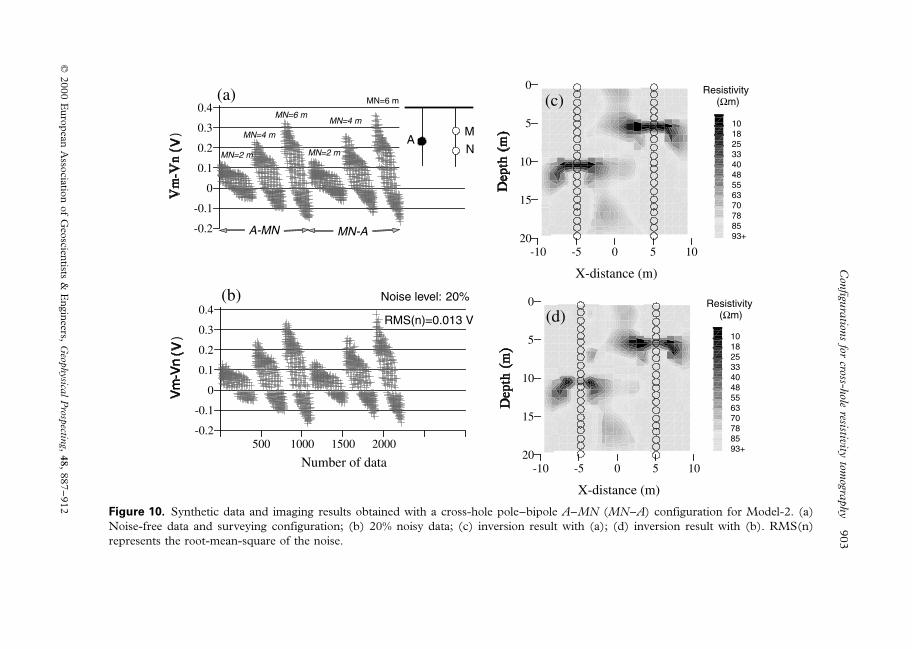
Figures 9 and 10 show another set of experiments with the cross-hole pole±bipoleA±MN (including MN±A) configuration. The synthetic data were also calculated with
the three separations of a pair of potential electrodes MN (MN 2 m, 4 m, 6 m) for
each current electrode A (see Figs 9a and 10a) with the symmetric geometries A±MNand MN±A. In order to enhance the spatial resolution of the configuration, we added
the logging data of the AMN configuration (the three electrodes are in the same
borehole) with the three spacings (these data are not given in Figs 9 and 10 due tomuch larger values than those shown in these figures). Thus, we have in total 2220
synthetic data for the imaging experiments. From these figures, we can see that thenoise-free data and 20% noisy data still yield very good images for Model-1 (see
Figs 9c and d), but for Model-2 the images are not as good as those obtained from the
A±M and AM±N configurations (compare Figs 10c and d with Figs 6c and d andFigs 8c and d). However, it should be noted that even though the inversions were
successful for Model-1, the synthetic data of the cross-hole A±MN (MN±A)
configuration involve much smaller voltages (max|VMN| , 0.35 V) than those ofthe configuration AM±N (N±AM) and there are many data close to zero with each
spacing (these are singularity points). It transpires that 275 and 265 data points were
rejected in the inversion of the noisy data for Model-1 and Model-2, respectively, due
Configurations for cross-hole resistivity tomography 897
q 2000 European Association of Geoscientists & Engineers, Geophysical Prospecting, 48, 887±912

-10 -5 0 5 10
X-distance (m)
0
5
10
15
20
101825334048556370788593+
-10 -5 0 5 10
X-distance (m)
0
5
10
15
20
101825334048556370788593+
0
2
4
6
500 1000 1500
Number of data
0
2
4
6
(a)
(b)
(c)
(d)
Resistivity(Ωm)
Resistivity
A-M M-A
AM
Noise level: 20%
RMS(n)=0.13 V(Ωm)
Figure 5. Synthetic data and imaging results obtained with a cross-hole pole±pole array for Model-1. (a) Noise-free data and surveyingconfiguration; (b) 20% noisy data; (c) inversion result with (a); (d) inversion result with (b). RMS(n) represents the root-mean-square ofthe noise.
89
8Z
.B
ing
and
S.A
.G
reenhalgh
q2
00
0E
uro
pean
Asso
ciation
of
Geo
scientists
&E
ngin
eers,G
eophysicalP
rospecting,
48,
88
7±
91
2

-10 -5 0 5 10
X-distance (m)
0
5
10
15
20
101825334048556370788593+
-10 -5 0 5 10
X-distance (m)
0
5
10
15
20
101825334048556370788593+
0
2
4
6
500 1000 1500
Number of data
0
2
4
6
(a)
(b)
(c)
(d)
Resistivity
Resistivity
A-M M-A
A M
Noise level: 20%
RMS(n)=0.13 V
(Ωm)
(Ωm)
Figure 6. Synthetic data and imaging results obtained with a cross-hole pole±pole array for Model-2. (a) Noise-free data and surveyingconfiguration; (b) 20% noisy data; (c) inversion result with (a); (d) inversion result with (b). RMS(n) represents the root-mean-square ofthe noise.
Con
figuration
sfor
cross-hole
resistivity
tomography
89
9
q2
00
0E
uro
pean
Asso
ciation
of
Geo
scientists
&E
ngin
eers,G
eophysicalP
rospecting,
48,
88
7±
91
2

-10 -5 0 5 10
X-distance (m)
0
5
10
15
20
101825334048556370788593+
-10 -5 0 5 10
X-distance (m)
0
5
10
15
20
10 to18 to25 to33 to40 to48 to55 to63 to70 to78 to85 to93+
0
2
4
6
500 1000 1500 2000
Number of data
0
2
4
6
(a)
(b)
(c)
(d)
AM=2 m
Noise level: 20%
Resistivity
Resistivity
AN
M
AM-N N-AM
RMS(n)=0.13 V
AM=4 m
AM=6 m
(Ωm)
(Ωm)
Figure 7. Synthetic data and imaging results obtained with a cross-hole pole±bipole AM±N (N±AM) configuration for Model-1. (a)Noise-free data and surveying configuration; (b) 20% noisy data; (c) inversion result with (a); (d) inversion result with (b). RMS(n)represents the root-mean-square of the noise.
90
0Z
.B
ing
and
S.A
.G
reenhalgh
q2
00
0E
uro
pean
Asso
ciation
of
Geo
scientists
&E
ngin
eers,G
eophysicalP
rospecting,
48,
88
7±
91
2

-10 -5 0 5 10
X-distance (m)
0
5
10
15
20
101825334048556370788593+
-10 -5 0 5 10
X-distance (m)
0
5
10
15
20
101825334048556370788593+
0
2
4
6
500 1000 1500 2000
Number of data
0
2
4
6
(a)
(b)
(c)
(d)Noise level:20%
Resistivity
Resistivity
AN
M
AM-N N-AM
RMS(n)=0.13 V
AM=2 m
AM=4 mAM=6 m
(Ωm)
(Ωm)
Figure 8. Synthetic data and imaging results obtained with a cross-hole pole±bipole AM±N (N±AM) configuration for Model-2. (a)Noise-free data and surveying configuration; (b) 20% noisy data; (c) inversion result with (a); (d) inversion result with (b). RMS(n)represents the root-mean-square of the noise.
Con
figuration
sfor
cross-hole
resistivity
tomography
90
1
q2
00
0E
uro
pean
Asso
ciation
of
Geo
scientists
&E
ngin
eers,G
eophysicalP
rospecting,
48,
88
7±
91
2

-10 -5 0 5 10
X-distance (m)
0
5
10
15
20
101825334048556370788593+
-10 -5 0 5 10
X-distance (m)
0
5
10
15
20
101825334048556370788593+
-0.15
-0.05
0.05
0.15
0.25
0.35
500 1000 1500 2000
Number of data
-0.15
-0.05
0.05
0.15
0.25
0.35
(a)
(b)
(c)
(d)
Noise level: 20%
Resistivity
Resistivity
A-MN MN-A
AN
M
MN=2 mMN=2 m
MN=4 m
MN=6 m MN=4 m
MN=6 m
RMS(n)=0.017 V
(Ωm)
(Ωm)
Figure 9. Synthetic data and imaging results obtained with a cross-hole pole±bipole A±MN (MN±A) configuration for Model-1. (a)Noise-free data and surveying configuration; (b) 20% noisy data; (c) inversion result with (a); (d) inversion result with (b). RMS(n)represents the root-mean-square of the noise.
90
2Z
.B
ing
and
S.A
.G
reenhalgh
q2
00
0E
uro
pean
Asso
ciation
of
Geo
scientists
&E
ngin
eers,G
eophysicalP
rospecting,
48,
88
7±
91
2
-10 -5 0 5 10
X-distance (m)
0
5
10
15
20
101825334048556370788593+
-10 -5 0 5 10
X-distance (m)
0
5
10
15
20
101825334048556370788593+
-0.2
-0.1
0
0.1
0.2
0.3
0.4
500 1000 1500 2000
Number of data
-0.2
-0.1
0
0.1
0.2
0.3
0.4
(a)
(b)
(c)
(d)Noise level: 20%
Resistivity
Resistivity
A-MN MN-A
AN
M
MN=2 m MN=2 m
MN=4 m
MN=4 mMN=6 m
MN=6 m
RMS(n)=0.013 V
(Ωm)
(Ωm)
Figure 10. Synthetic data and imaging results obtained with a cross-hole pole±bipole A±MN (MN±A) configuration for Model-2. (a)Noise-free data and surveying configuration; (b) 20% noisy data; (c) inversion result with (a); (d) inversion result with (b). RMS(n)represents the root-mean-square of the noise.
Con
figuration
sfor
cross-hole
resistivity
tomography
90
3
q2
00
0E
uro
pean
Asso
ciation
of
Geo
scientists
&E
ngin
eers,G
eophysicalP
rospecting,
48,
88
7±
91
2

to serious contamination by noise. In fact, the RMS value of the noise
(RMS(n) 0.013 V) in the experiments is much smaller than that of the cases
with A±M and AM±N configurations (RMS(n) 0.13 V). This means that whateverspacing is used in cross-hole profiling, such weak values obtained with the A±MN(MN±A) configuration are easily masked by the background noise. In addition, the
inferiority of imaging with Model-2 indicates that the horizontal resolution of theconfiguration is not as good as that of the pole±pole and AM±N configurations.
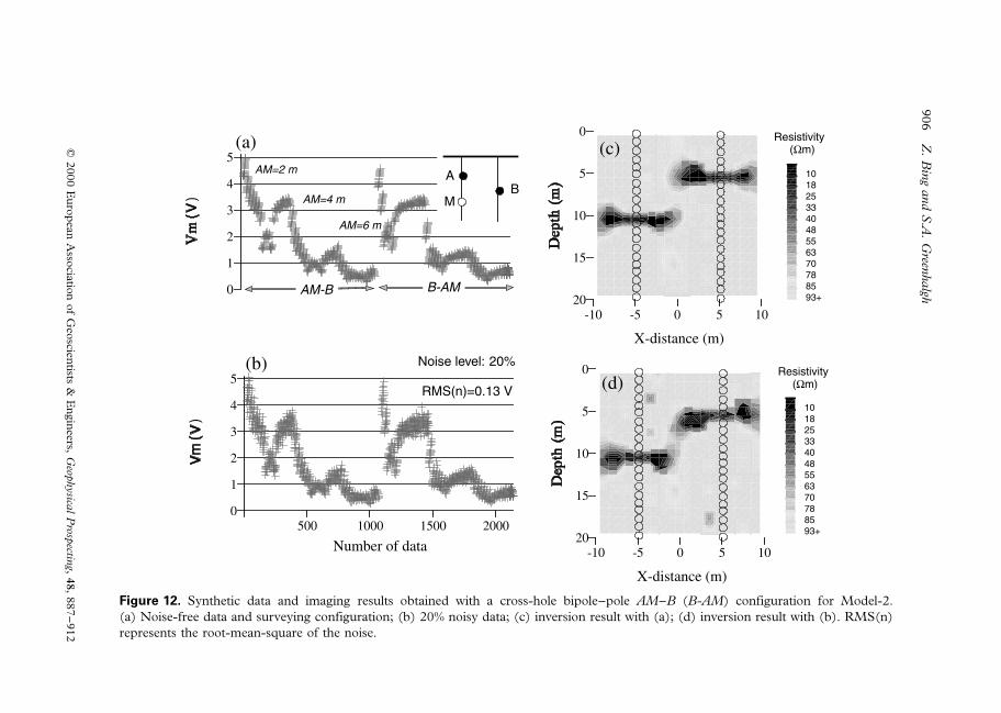
3 Bipole±pole array
In the six independent configurations of the cross-hole bipole±pole surveying (seeFig. 2), only two, AM±B and AB±M, may be considered as representative of these
configurations, because the others are similar to them or simply their symmetric
counterparts. According to the reciprocity principle, the configuration AB±M isequivalent to MN±A, which has already been tested for imaging the two models (see
Figs 9 and 10). Here, we employ the bipole±pole AM±B (including B±AM)
configuration to conduct the numerical experiments. Figures 11 and 12 show thesynthetic data and the imaging results for the two models. The synthetic data were
calculated with three separations of the pair of electrodes AM (AM 2 m, 4 m, 6 m)
for each current electrode B, so we have 2142 data points for the imaging (seeFigs 11a and b and Figs 12a and b). From these figures we can see that the potential
responses are very similar to those with the AM±N configuration (i.e. see Figs 7a and
11a) and the data range is still comparable to that with the pole±pole configuration(0.25,5 V, RMS(n) 0.13 V for 20% noise). The inversion results show that the
bipole±pole AM±B configuration can yield very clear images for the two models even
when using the noisy data. Comparing these images with the previous resultsproduced by the pole±pole (Figs 5 and 6), pole±bipole AM±N (Figs 7 and 8) and
A±MN configurations (Figs 9 and 10), we see that this configuration produces nearly
the same quality images of the models as the pole±pole A±M and pole±bipole AM±Nconfigurations, and much better images than that of the A±MN configuration.
4 Bipole±bipole array
The cross-hole bipole±bipole array has only three independent surveying configura-tions: AM±BN, AM±NB and AB±MN (see Fig. 3). Firstly, we tested the imaging
effectiveness with the AM±BN configuration. Figures 13 and 14 show the synthetic
data and the imaging results for the two models. In computing the synthetic data, theseparation of a pair of electrodes BN is kept the same as AM (AM BN a) to give
a symmetric geometry and three separations of the two electrodes AM(AM BN 2 m, 4 m, 6 m) are employed (see Figs 13a and 14a). In total, 875data (a much smaller number of data than the other configurations) were inverted for
the imaging experiments. From the synthetic data (Figs 13a and 14a), we can see that
each spacing of the configuration has a different range of the `observed' values. The
904 Z. Bing and S.A. Greenhalgh
q 2000 European Association of Geoscientists & Engineers, Geophysical Prospecting, 48, 887±912

-10 -5 0 5 10
X-distance (m)
0
5
10
15
20
101825334048556370788593+
-10 -5 0 5 10
X-distance (m)
0
5
10
15
20
101825334048556370788593+
0
1
2
3
4
5
500 1000 1500 2000
Number of data
0
1
2
3
4
5
(a)
(b)
(c)
(d)
AM=2 m
Resistivity
Resistivity
AM-B B-AM
AB
M
Noise level: 20%
RMS(n)=0.13 V
AM=4 m
AM=6 m
(Ωm)
(Ωm)
Figure 11. Synthetic data and imaging results obtained with a cross-hole bipole±pole AM±B (B-AM) configuration for Model-1.(a) Noise-free data and surveying configuration; (b) 20% noisy data; (c) inversion result with (a); (d) inversion result with (b). RMS(n)represents the root-mean-square of the noise.
Con
figuration
sfor
cross-hole
resistivity
tomography
90
5
q2
00
0E
uro
pean
Asso
ciation
of
Geo
scientists
&E
ngin
eers,G
eophysicalP
rospecting,
48,
88
7±
91
2
-10 -5 0 5 10
X-distance (m)
0
5
10
15
20
101825334048556370788593+
-10 -5 0 5 10
X-distance (m)
0
5
10
15
20
101825334048556370788593+
0
1
2
3
4
5
500 1000 1500 2000
Number of data
0
1
2
3
4
5
(a)
(b)
(c)
(d)
Resistivity
Resistivity
AM-B B-AM
AB
M
Noise level: 20%
RMS(n)=0.13 V
AM=2 m
AM=4 m
AM=6 m
(Ωm)
(Ωm)
Figure 12. Synthetic data and imaging results obtained with a cross-hole bipole±pole AM±B (B-AM) configuration for Model-2.(a) Noise-free data and surveying configuration; (b) 20% noisy data; (c) inversion result with (a); (d) inversion result with (b). RMS(n)represents the root-mean-square of the noise.
90
6Z
.B
ing
and
S.A
.G
reenhalgh
q2
00
0E
uro
pean
Asso
ciation
of
Geo
scientists
&E
ngin
eers,G
eophysicalP
rospecting,
48,
88
7±
91
2

200 400 600 800
Number of data
0
2
4
6
8
10
-10 -5 0 5 10
X-distance (m)
0
5
10
15
20
1018263543515967758492100+
-10 -5 0 5 10
X-distance (m)
0
5
10
15
20
101825334048556370788593+
0
2
4
6
8
10(a)
(b)
(c)
(d)
Resistivity
Resistivity
a=2 m a=4 m a=6 m
A B
M Na a
Noise level: 20%
RMS(n)=0.28 V
(Ωm)
(Ωm)
Figure 13. Synthetic data and imaging results obtained with a cross-hole bipole±bipole AM±BN configuration for Model-1. (a) Noise-freedata and surveying configuration; (b) 20% noisy data; (c) inversion result with (a); (d) inversion result with (b). RMS(n) represents theroot-mean-square of the noise.
Con
figuration
sfor
cross-hole
resistivity
tomography
90
7
q2
00
0E
uro
pean
Asso
ciation
of
Geo
scientists
&E
ngin
eers,G
eophysicalP
rospecting,
48,
88
7±
91
2

-10 -5 0 5 10
X-distance (m)
0
5
10
15
20
101825334048556370788593+
-10 -5 0 5 10
X-distance (m)
0
5
10
15
20
101825334048556370788593+
0
2
4
6
8
10
200 400 600 800
Number of data
0
2
4
6
8
10
(a)
(b)
(c)
(d)
a=2 m
Resistivity
Resistivity
a=4 m a=6 m
A B
M Na a
Noise level: 20%
RMS(n)=0.28 V
(Ωm)
(Ωm)
Figure 14. Synthetic data and imaging results obtained with a cross-hole bipole±bipole AM±BN configuration for Model-2. (a) Noise-freedata and surveying configuration; (b) 20% noisy data; (c) inversion result with (a); (d) inversion result with (b). RMS(n) represents theroot-mean-square of the noise.
90
8Z
.B
ing
and
S.A
.G
reenhalgh
q2
00
0E
uro
pean
Asso
ciation
of
Geo
scientists
&E
ngin
eers,G
eophysicalP
rospecting,
48,
88
7±
91
2

small spacing gives relatively large values, while the large spacing has relatively small
ones. To obtain high signal/noise ratio data, the spacings may be adapted to the real
applications according to the separation of the boreholes and the level of backgroundnoise. The multiple spacings are necessary for the imaging, because with an increase
in the electrode spacing we may obtain more information on the horizontal electric
properties. This option provides greater flexibility in cross-hole surveying. From theimaging results (see Figs 13c and d and Figs 14c and d), we can see that although
the total number of data (875) is much smaller than for the other configurations and
the RMS value of the noise (RMS(n) 0.28 V for 20% noise) is double that of theprevious cases, the AM±BN configuration produces satisfactory images of the two
models. We repeated the experiments with different values of the three spacings and in
most cases they gave the same imaging results as shown in Figs 13 and 14.From Fig. 3, it is clear that the bipole±bipole configurations AM±BN and AM±NB
do not differ much in field geometry. From numerical tests of the two models, we
found that the bipole±bipole AM±NB configuration (see Fig. 3b) has very similarresults to those shown in Figs 13 and 14 which were obtained with the configuration
AM±BN. This implies that the two bipole±bipole configurations are not very different
in cross-hole resistivity tomography.Another cross-hole bipole±bipole configuration, AB±MN (see Fig. 3c), which
involves having both current electrodes in the same borehole and both potential
electrodes in the other borehole, has been investigated because of the significantdifference in data acquisition. We calculated the potential difference (VM 2 VN) with
three spacings (AB MN a 2 m, 4 m, 6 m) and obtained the same number of
data (875) for the tests. It was found that the potential difference (VM 2 VN) for thisconfiguration is generally much smaller (, 0.35 V) than for the AM±BN configuration,
and the configuration has the same singularity problem as the A±MN configuration ±many data are close to zero in cross-hole profiling with each spacing. In the inversion
procedure, 173 data and 219 data were rejected due to the serious noise contamination.
The imaging results (omitted here) show many artefacts in the images of Model-1 and apoor image for Model-2 even with the weak noise (RMS(n) 0.005 V for 20% noise).
In summary, these imaging results show that the images yielded by the pole±pole,
pole±bipole AM±N, bipole±pole AM±B and bipole±bipole AM±BN configurationsare very competitive with 20% noisy data. Theoretically, the pole±pole noise-free data
should produce the best image of all these configurations, because the complete pole±
pole data set contains maximum information on the electric properties aroundboreholes and the other configuration data sets may be derived from them. However,
the better anomaly effects and different sensitivity patterns of the three- and four-
electrode configurations (Zhou and Greenhalgh 1997) may compensate for theincomplete information from the data. This may be why these three- and four-
electrode configurations yield images of comparable quality to the pole±pole array. By
conducting additional numerical experiments for imaging high-contrast anomalies ofthese same two models (the resistivities of the anomaly and the host medium are
10 Vm and 1000 Vm, respectively), we obtained similar results.
Configurations for cross-hole resistivity tomography 909
q 2000 European Association of Geoscientists & Engineers, Geophysical Prospecting, 48, 887±912
In addition, the synthetic data (simulation of cross-hole measurement) show us that
the pole±bipole A±MN, bipole±pole AB±M and bipole±bipole AB±MN configura-
tions, besides having a singularity problem in the computation of apparent resistivity(Zhou and Greenhalgh 1997), may produce small observed quantities (potential VM
or potential difference (VM 2 VN)) in practical applications. These small voltages
may easily be masked by the background noise. The imaging capabilities of theseconfigurations are not as good as the pole±pole, pole±bipole AM±N, bipole±pole
AM±B and bipole±bipole AM±BN configurations.
Conclusions
For cross-hole resistivity tomography, the synthetic imaging experiments demonstratethat, besides the pole±pole array, some specific three- and four-electrode configura-
tions, such as AM±N, AM±B and AM±BN, can be efficiently employed. These
configurations, compared with the cross-hole pole±pole survey, have some distinctadvantages in the field measurements, better anomaly effects and different sensitivity
patterns so that they may produce competitive images with 20% noisy data.
Specifically, the cross-hole bipole±bipole AM±BN configuration has the followingadvantages: (i) no remote-electrode effects, (ii) it completely satisfies reciprocity, (iii)
adjustable sensitivity with different electrode spacing and (iv) easy acquisition of field
data in built-up areas. These kinds of measurement configurations yield greaterflexibility for cross-hole resistivity tomography in practice.
The cross-hole pole±bipole A±MN, bipole±pole AB±M and bipole±bipole AB±
MN configurations have a singularity problem in data acquisition ± involving manynear-to-zero potential values in cross-hole profiling with any spacings. For practical
applications, it will lead to many low readings of the potential or potential difference
which can easily be obscured by background noise. The numerical simulations showthat the effectiveness of cross-hole resistivity tomography with these configurations is
not as good as with the other arrays.
Acknowledgements
This work was supported by an Overseas Postgraduate Research Scholarship and anAdelaide University Research Scholarship to Z.B. at The University of Adelaide,
Australia. We are grateful to the Australian Research Council and to the CSIRO
Center for Groundwater Studies for funding the project. Two anonymous reviewersand Associate Editor, Pierre Valla, provided constructive criticisms.
References
Constable S.C., Parker R.L. and Constable C.G. 1987. Occam's inversion: a practical algorithm
for generating smooth models from electromagnetic sounding data. Geophysics 52, 289±300.
910 Z. Bing and S.A. Greenhalgh
q 2000 European Association of Geoscientists & Engineers, Geophysical Prospecting, 48, 887±912

Dabas M., Tabbagh A. and Tabbagh J. 1994. 3D inversion subsurface electrical surveying ± I.
Theory. Geophysical Journal International 119, 975±990.
Daily W. and Owen E. 1991. Cross-borehole resistivity tomography. Geophysics 56, 1228±1235.
Daniels J.J. 1977. Three-dimensional resistivity and induced-polarisation modeling using buried
electrodes. Geophysics 42, 1006±1019.
Daniels J.J. and Dyck A. 1984. Borehole resistivity and electromagnetic methods applied to
mineral exploration. IEEE Transactions on Geoscience and Remote Sensing GE-22, 80±87.
Ellis R.G. and Oldenburg D.W. 1994a. Applied geophysical inversion. Geophysical Journal
International 116, 5±11.
Ellis R.G. and Oldenburg D.W. 1994b. The pole±pole 3D-resistivity inverse problem: a
conjugate-gradient approach. Geophysical Journal International 119, 187±194.
Kennett B.L.N. and Williamson P.R. 1988. Subspace methods for large-scale non-linear
inversion. In: Mathematical Geophysics, a Survey of Recent Developments in Seismology and
Geodynamics (eds N.J. Vlaar, G. Nolet, M.J.R. Wortel and S.A.L. Cloetingh), pp. 139±154.
D. Reidel, Dordrecht.
LaBrecque D., Miletto M., Daily W., Ramirez A. and Owen E. 1996. The effects of `Occam'
inversion of resistivity tomography data. Geophysics 61, 538±548.
Li Y.G. and Oldenburg D.W. 1992. Approximate inverse mapping in DC resistivity problems.
Geophysical Journal International 109, 343±362.
Loke M.H. and Barker R.D. 1995. Least-squares deconvolution of apparent resistivity
pseudosections. Geophysics 60, 1682±1690.
Loke M.H. and Barker R.D. 1996. Rapid least-squares inversion of apparent resistivity
pseudosections by a quasi-Newton method. Geophysical Prospecting 44, 131±152.
Militer H., Rosler R. and Losch W. 1979. Theoretical and experimental investigations for cavity
research with geoelectrical resistivity methods. Geophysical Prospecting 27, 640±652.
Oldenburg D.W. and Li Y. 1994. Inversion of induced polarization data. Geophysics 59, 1327±
1341.
Oldenburg D.W., McGillicray P.R. and Ellis R.G. 1993. Generalised subspace methods for
large-scale inverse problems. Geophysical Journal International 114, 12±20.
Owen E. 1983. Detection and Mapping of Tunnels and Caves. Development in Geophysical
Exploration Method ± 5. Applied Science Publishers.
Park S.K. and Van G.P. 1991. Inversion of pole±pole data for 3D resistivity structure beneath
arrays of electrodes. Geophysics 56, 951±960.
Pelton W.H., Rijo L. and Swift C.M., Jr 1978. Inversion of two-dimensional resistivity and
induced-polarization data. Geophysics 43, 788±803.
Sasaki Y. 1994. 3D resistivity inversion using the finite element method. Geophysics 59, 1839±
1848.
Shima H. 1992. 2D and 3D resistivity imaging reconstruction using cross-hole data. Geophysics
55, 682±694.
Skilling J. and Bryan R.K. 1984. Maximum entropy image reconstruction, general algorithm.
Monthly Notices of the Royal Astronomical Society 211, 111±124.
Smith N.C. and Vozoff K. 1984. Two-dimensional DC resistivity inversion for dipole-dipole
data. IEEE Transactions on Geoscience and Remote Sensing GE-22, 21±28.
Tarantola A. and Vallette B. 1982. Generalized non-linear inverse problem solved using the
least-squares criterion. Reviews of Geophysics and Space Physics 20, 219±232.
Configurations for cross-hole resistivity tomography 911
q 2000 European Association of Geoscientists & Engineers, Geophysical Prospecting, 48, 887±912

Tripp A.C., Hohmann G.W. and Swift C.M., Jr 1984. Two-dimensional resistivity inversion.
Geophysics 49, 1708±1717.
Van G.P., Park S.K. and Hamilton P. 1991. Monitoring leaks from storage ponds using
resistivity methods. Geophysics 56, 1267±1270.
Xu B. and Noel M. 1993. On the completeness of data sets with multi-electrode systems for
electrical resistivity survey. Geophysical Prospecting 41, 791±801.
Zhang J., Mackie R. and Madden T. 1995. 3D resistivity forward modeling and inversion using
conjugate gradients. Geophysics 60, 1313±1325.
Zhou B. 1998. Cross-hole resistivity and acoustic velocity imaging: 2.5D Helmholtz equation
modeling and inversion. PhD thesis, University of Adelaide.
Zhou B. and Greenhalgh S. 1995. A fast approach to FreÂchet derivative computation for
resistivity imaging with different electrode arrays. Geotomography, vol. III: Fracture Imaging,
pp. 252±264. Society of Exploration Geophysicists of Japan.
Zhou B. and Greenhalgh S.A. 1997. A synthetic study on cross-hole resistivity imaging with
different electrode arrays. Exploration Geophysics 28, 1±5.
Zhou B. and Greenhalgh S.A. 1999. Explicit expressions and numerical calculations for the
FreÂchet and second derivatives in 2.5D Helmholtz equation inversion. Geophysical Prospecting
47, 443±468.
Zienkiewicz O.C. 1971. The Finite Element Method in Engineering Science. McGraw-Hill Book
Co.
912 Z. Bing and S.A. Greenhalgh
q 2000 European Association of Geoscientists & Engineers, Geophysical Prospecting, 48, 887±912