Reporl No. 316a-TU

The Economic Development FILE COPYof Turkey(In Five Volumes)

Volume IV: Technical AnnexApril 22, 1974

Country Programs Department IIEurope, Middle East and North Africa Region

Not for Public Use

Document of the International Bank for Reconstruction ancl DevelopmentInternational Development Association

This report was prepared for official use orly by the Bank Group. It may not be published.quoted or cited without Bank Croup authorization. The Bank Group does not accept responsibilityfor the accuracy or completeness of the report.

Pub

lic D

iscl

osur

e A

utho

rized

Pub

lic D

iscl

osur

e A

utho

rized

Pub

lic D

iscl

osur

e A

utho

rized

Pub

lic D

iscl

osur

e A

utho

rized

Pub

lic D

iscl

osur

e A

utho

rized

Pub

lic D

iscl

osur

e A

utho

rized

Pub

lic D

iscl

osur

e A

utho

rized

Pub

lic D

iscl

osur

e A

utho

rized

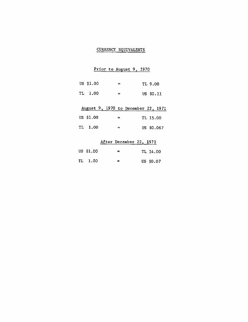
CURRENCY EQUIVALENTS

Prior to August 9, 1970

US $1.00 = TL 9.00

TL 1.00 = US $0.11

August 9, 1970 to December 22, 1971

US $1.00 = TL 15.00

TL 1.00 = US $0.067

After December 22, 1971

US $1.00 = TL 14.00

TL 1.00 = US $0.07

VOLUME IV

TBEHNICAL ANNEX

Table of contents

Page No.

Chapt. 14 ANALYSIS OF MEDIUM AND LONG TERMGROWTH PERSPECTIVE ***.*******..................... 1

Introduction .............................. 1

A. Growth and Enployment Perspective, 1972-87 .... 1A Perspective Planning Model for Turkey .... 2Basic Solution for 1987 ....................... 3Alternative Growth Patterns ................... 20Annex Al: Date Base for the Linear Programning

Model .ooo.......... ....Annex A2: Further Improvement of the Model ...

B. A Two-Gap Model for the Turkish Economy ..... 2.. 5Annex B1: Structure of the Model

Chapter 14

ANALYSIS OF MEDIUM AND LONG TERM GROWTH PERSPECTIVES

Introduction

14.1 Growth of the Turkish economy has been impressive in the last twodecades. Turkey has reached a per capita income of $420 in 1972 compared toabout $230 in 1950 in 1972 dollars, and is entering a new phase of developmentwhich should lead to a more radical transformation of its economic structure.The Government has recently adopted a new 22-year development strategy, withthe aim of reaching a per capita income of about $1500 by 1995 while becominga full member of the European Common Market. A fast industrialization andurbanization would bring the economy to the stage of development of Italy in1970. Past performance and the natural and human resources of the countryindicate that this expected radical transformation could be achieved. However,Turkey would have to overcome basic constraints and find the solution to manyproblems and imbalances. While growth in the last twenty years has been cha-racterized by nearly continuous foreign exchange shortages and inflationarypressure, the main problems of the next twenty years are likely to be employ-ment creation, income distribution and economic management, particularly demandmanagement.

14.2 Macroeconomic models are usually not fit for exploring all aspectsof economic development, but focus on some specific problems. We have ex-plored some aspects of the long-term growth of the Turkish economy with twomodels. These models are not substitutes to the long-term model prepared bySPO but rather are devised to focus on specific aspects of the economy andadd to our knowledge of its potentials and constraints. With a linear pro-gramming dynamic model, we have explored the( link between optimum growth pat-terns following various criteria and employment growth. With a two-gap HarrodDomar type model, we have explored the link between growth, inflation and thebalance of payments. The programming model has been developed with the coop-eration of the Development Research Center of the Bank, and data were partlysupplied in Turkey by the SPO. The two-gap model has been developed in coop-eration with the Comparative Analysis and Projections division of the Bank.The possibilities of linking the two models in a systematic way have not beenexplored, but the two sets of projections are consistent. Both are based onthe same Turkish statistics, and the linear programming model uses as exogenousvariable the foreign exchange availabilities obtained endogenously in the two-gap model. The results of the two models can.add insight into the possiblelong-term development trends of the economy, but the magnitudes should notbe considered as predictive of the future.

A. Growth and Employment Perspectives of the Turkish Economy, 1972-87An Exploration of Optimum Patterns

14.3 The object of this chapter is to analyze some of the results obtainedfrom a linear programming model of the Turkish economy developed by Charles R.Blitzer of the Development Research Center, IBRD, in 1970, who also contributedsubstantially to this exercise. The first section describes briefly the majorcharacteristics of the model, the second section describes for 1987 some ofthe informations generated by the model in a basic case, with particular

-2-

emphasis on sectoral production and investments, and the volume and composi-tion of labor skill. The third section will analyze various types of trade-offs between different development objectives. The description of how thedata base of the model developed by C. Blitzer has been updated from infor-mations collected during the basic mission, and of possible further improve-ments in the model are given in Annexes.

A Perspective Planning Model for Turkey -

14.4 This dynamic multi-sector model has been built to explore the linkbetween the pattern and pace of growth and employment in the Turkish economy.The model maximizes a given function (GDP, consumption or employment) foreach of five three-year periods, during 1972-1987, starting with the period1972-75. Growth of the economy is bound by labor constraints, material con-straints and foreign exchange and savings constraints. All projections aregiven in 1972 prices and start from 1972 as a base year, for which an inputoutput table, a transaction matrix and a capital coefficients matrix havebeen estimated by the Bank mission, in close cooperation with the DevelopmentResearch Center of the Bank and the SPO in Turkey. (Tables Al to A4).

14.5 The economy is divided in eight sectors, and labor forces in eachsector into six skill categories (Table A17). Turkey is considered as a laborsurplus economy only for unskilled labor in agriculture (skill 6). The laborconstraints ensure that availability of each skill level in each time periodof the projection meets the various requirements. For skills 1 to 4, laborsupply can come from three sources: 1) an exogenous supply of skilled laborby the existing education system (Table All), 2) upgrading of l1,wer skilllevels through a human capital formation activity starting in previous periodsand obtained at an investment cost for the economy (Table A4), and 3) down-grading of upper skill levels in excess supply. Additions to unskilled urbanlabor (skill 5) come from urban rural migration, and cost to the economy TL2,900 per year and per migrant in 1972 prices 2/ (Table A9). Labor demand bysector is derived from an analysis of labor requirements per unit of outputin 1972, and is prpjected after accounting for exogenous changes in produc-tivity (Tables A10, A12). Skill composition of the increase in labor forcein each sector is kept constant overtime, but is different from the initialskill composition, and the changes of the skill mix of labor force overtimeare due to changes in productivity and different sectoral grorwth rates. 3/

1/ For a detailed presentation of the model and its equations, refer to "APerspective Planning Model for Turkey: 1969-1984", Charles R. Blitzer,Memorandum No. 114, Research Center in Economic Growth, Stanford Univer-sity, California (August 1971).

2/ The question of who should bear the cost of these migrations has notbeen envisaged in this study.

3/ Introducing income elasticities of labor productivity is not possibleat this stage for lack of statistical information.

- 3 -

14.6 Material Constraints (Bit). In each sector of the economy, materialconstraints ensure that for each time period resources (imports plus output)meet the demand for consumption, investment, export and migration costs.

14.7 Foreign Exchange Constraints (Ct). For each time period, foreignexchange earnings (exports, net foreign capital, workers' remittances) mustmeet the demand for imports of consumer goods, intermediate raw material andcapital goods and of increase in reserves. Imports have been divided in eachsector into competitive and noncompetitive in the dynamic sense, noncompetitiveimports being those imports which Turkey is unlikely to produce at internationalcost within the projection period. The model allows for import substitutionin the field of competitive imports only, and there are rigid import coeffi-cients for noncompetitive imports. Exports are divided into five categories,which is clearly too aggregated for a detailed study of comparative advantages,and each category is bound by an upper and a lower growth rate limit. Thelevel of net foreign aid, workers' remittances and net changes in reservesare exogenous, and take into account the Turkish objective of less dependenceon foreign resources and the balance of payments analysis carried out with atwo-gap model (see part B and Table A16).

14.8 Savings Constraint. The marginal propensity to save is constrainedby an upper limit taken as 26Z for domestic savings for the basic case.

Basic Solution for 1987

14.9 The basic case of the programming model has been solved by maximimiz-ing GDP in the terminal year. 1/ It will serve as a benchmark from which trade-offs between various objectives and formulations will be measured.

14.10 Macroeconomic Results. The major macroeconomic results are presentedin Table 76. The growth rate of GDP is projected to be 7.2% during 1972-87.Investment grows at 8.5% per year, and domestic savings increase at 10.2%per year, the marginal savings remaining always at their upper limit. In1987, investment reaches 24.5% of GDP and domestic savings 22% of GDP, com-pared to 20.4% and 14.6% respectively in 1972 (with the same definition ofGDP). Per capita consumption increases by 4.1% per year during the period.The incremental capital output ratio averages 3.32. The reorganization ofthe economy towards the optimum pattern of growth which occurs in the earlyyears explains the low growth rate of GDP in 1972-75, the slightly decreasingICRO, and some peculiar sectoral growth rates of investment during this period,particularly in transport and agriculture, which should not be taken as nor-mative.

1/ Terminal and post terminal conditions have been set up on GDP, consump-tion, and investment to avoid the end projection disturbances normallyassociated with programming models.

- 4 -

Table 71_ Summary of constraint rows

Constraint.group Definition Number of rows

Ast labor balances 25

Bit material balances 40

Ct foreign exchange balances 5

Eit output capacity 40

Fst education capacity 15

Gzt upper bounds on exports 25

-Hzt lower bounds on exports 25

Ilit sectoral investment levels 48

it aggregate investment levels 6

TXi,t sectoral.gross output 40

St marginal propensity to 5consume

ACt total consumption 5

,GDPt grossAdomestic product .5

C6 terminal consumption I

Ki terminal investment levels 8

Ks terminal education levels 4

OBJ .objective function 1

298

Table 72: Sumr f Act:ivity Columns

activity type number of activitycolumns

Ct per capita consumption increase 6between base year and period t;unit: 1963 TL

XJ t gross output increment in sector j 40between base year and period t(j=1,...,8;t-l,...,5); unit: billionsof 1963 TL

VJ,t annual increase in capacity of sector 66j during time period t (j=l,...,ll;tO0,...,5) N.B. sectors 9,10, and 11 areeducation sectors; unit: billions of1963 TL

Mit annual "competitive" imports of item i 15during time period t(i=1,2,3;t=l,...,5); unit: billions of1963 TL

Z annual earnings from export activity 25z during time period t(z=1,...,5;t-1,...,5); unit: billionsof 1963 TL

MLt level of migration during period t 5unit: thousands of persons

EDj Jt level of education activity j during 20the time period t(j=1,...,4;t-1,...,5); ullit: thousandsof persons

LD J,t labor downgraded from skill level j 20during period t(J=l,...,4;t=l,...,5); unit: thousandsof persons

IJ,t annual investment level in sector j 48during period t (j-l,...,8;t-0,1,...,5);unit: billions of 1963 TL

TX ilt annual gross output level in sector j 40during period t (j.1,...,8;t'1 ,...,5);unit: billions of 1963 TL

AC annual total consumption during period 5t t (t=l,...,5); unit: billions of 1963 TL

It annual total investment level during period 5t (t=l,... ,5); unit: billions of 1963 TL

GDPt annual level of gross domestic product during 5period t (t=l,...,5); unit:billions of 1963 TL

300

-6-

Table-73: (Ast) Constraints:

requirement requirementfor skill for skilllevel s in + level s in Lproductive production ofsectors human capital

8 o ~~8 4(Ls0 _ I 10 : TXj O) + I lS, TXj,t + I 1'5 ED, JtB'O J-1 ~~J=1 j=l

exogenous net additions and losses net gains Rrban-ruralsupply, time + from training activities + from down- + migration;t in prior periods j grading only for s=5

+ t-F1 + [EDs. - ED *1 + LDs-t - LDst + I MLT=1 , -, , Tla

Table 74: (Bit) Constraints:

,year 0_ increase + :=netitive" output, net + -above base porto i-1,2,3 >of induftry year output,demand - net of industry

demand

8L+ I ai,j j,t I xi,t -

opulatio g capita 1 + investmenFl + export + migration-L J~~1 sumption L demand J Ldemandj Losts J

E12 -1 1, ,t + It t 5 tFt [ C±,O + ci CtI+ bj VJ' + +m i J'i Tm jinl in

Table 75: (Ct) Constraints

Fpopulation base year increase in intermediate increase in capital good "competitive"

Epo ~ ~per capita + per capita + imports, base + intermediate + imports + imports above _

consumption consumption year good imports minimum levels of imports of imports L I __

8 11 3

Pt (C= o + c=Ct) + + m x + u V + mj '

export net foreign workers'

L l time t and otherinvisibles

5

jIl Ji1 t +

Table 76- Macroaeonomic Projections (Basic Case)

1972 1975 1978 1981 1984 1987

GDP 207.1 L 249.5 306.5 377.2 471.9 590.4

Consumption 176.8 208.2 250.3 302.7 372.7 460.4

Per capitaUnit: consumption 4753 5183 5787 65-15 7516 8725

(1972 TL)billions

Net capital1972 inflow, changes 11.9 13.3 16.3 15.5 14.8 14.5

in reserves andTL invisibles

Domesticsavings 30.3 41.3 56.2 74.5 99.2 130.0

Inveatuent 42.2 54.6 72.4 90.0 113.9 144.5

1972-87

GDP 6.4 7.1 7.2 7.8 7.8 7.2

Unit: Consumption 5.6 6.3 6.5 7.2 7.3 6.6

anmual Dmoesticsavings 10.9 10.8 9.8 10.0 9.4 10.2

gmp thInvestment 8.9 9.9 7.5 8.2 8.2 8.5

ratesMarginalpropensity .26 .26 .26 .26 .26 .26to save

Incementalcapital- 3.42 3.43 3.44 3.23 3.27 3.32output ratio

/ In the preparation of the 1972 transaction matrix and input-output table, taxes on imports have beenadded to CIF imports, which then gives a slightly different definition of gross value odded thannormally adjusted (207.1 instead of 215.7 by SIS).

- 10 -

14.11 The long-term growth targets for 1972-87 in the new developmentstrategy of the Turkish Government are more ambitious; GDP is assumed to growat 8.7% per year, investment 11.7%, domestic savings at 11.8% and per capitaconsumption at 4.9%. The lower estimates obtained in the programming modelare mainly due to a lower marginal propensity to save (26% instead of 38%),the existence of labor constraints and migration costs (Table A9) and to adifferent growth pattern and investment allocation.

14.12 Sectoral Growth and Investment Allocation (Tables 77 and 78). Theoptimum growth pattern for 1972-87 emphasizes industrialization and utilities,while agriculture and services grow slower. However, this growth pattern ismore balanced than in the past, and more balanced than the growth pattern pro-posed in the new development strategy, with a faster growth in agriculturaloutput than in the long-term strategy (5.6% instead of 5.1%), and a slowergrowth in all the other sectors, particularly mining (6.9% instead of 12.9%),construction (7.2% instead of 10.7%) and utilities (8.6% instead of 11.9%).

14.13 The investment allocation which leads to this growth pattern con-tinues the past emphasis on industrialization, but with less accelerationthan in the long-term strategy of the Government, more concern for the agri-cultural sector and less investment in the transport sector. Compared to thepast investment structure, the share of investment in agriculture increases(about 15% compared to 13% during 1963-72), the share in industry increases(about 40% compared to 35%), and the share in services decreases (45% comparedto 52%). In the long-term strategy of the Government, the share of industryincreases faster to 48%, while both the shares of agriculture and services(10% and 42% respectively) decrease.

14.14 Labor Situation (Tables 79 and 80). Manpower requirements by skilland time period are described in Table 77, and educational requirements andskill downgrading and upgrading are described in Table 78. The pace and pat-tern of growth described in the previous paragraphs require a yearly growthof skilled labor of 5.0%, the fastest growth being in skill 3 (administrativeand clerical) and 1 (university level). The requirements for unskilled urbanmanpower lead to the migration of nearly three million persons from the ruralareas, or 200,000 persons per year. Total urban labor force is defined as thesum of the exogenous urban labor force (increasing at 2.5% per annum) andrural-urban migration, and is engaged both in production and the creation ofhuman capital. Hence, the differences between the total manpower requirementsand the urban labor force is attributable to the education and training ac-tivities. For example, in 1978, 5912 thousand man/years are required by theeight production sectors, while the urban labor force totals 6039. The dif-ference of 127 thousand man/years represents labor being utilized in humancapital creation.

14.15 The long-term strategy of the Government estimates an urban laborforce of 13 million in 1987, and a demand for labor of 11 million, leaving2 million urban unemployed. The programming model indicates that urban em-ployment would amount to 9.7 million, leaving 3.3 million urban unemployed,or 34% of urban labor force. Employment requirements lower than expectedmight slow down rural-urban migrations and therefore urban labor force andunemployment, but these estimates indicate that the problem to be solvedseems more serious than expected in the Government strategy.

- 11 -

Table 77: Gross output projections (Basic Case)

(units: average annual growth rates and billions of 1972 TL)

Sector Gross output, Gross output, Average annual Average annual1972 '987 rate of growth rate of growth

1963-1972 L 1972-1987

1. Agriculture 83.3 189.4 3.6 5.6

2. Mining 5.6 15.2 6.7 6.9

3. Manufacturing 117.1 408.8 10.6 8.7

4. Utilities 6.6 22.9 9.9 8.6

5. Constraction 27.1 77.2 6.6 7.2

6. Commerce 27.3 80.2 9.1 7.5

7. Transportation 24.1 73.7 7.9 7.7

8. Services 63.1 160.2 6.3 6.4

Total 354.2 1027.6 6.6 7.3

A Growth rate of value added at factor cost.

- 12 -

table 78:- Percentage composition of investment by sector of destination (Basic Case)

Sector 1972-' 1975-' 1978 1981 1984

1. Agriculture 11.1 16.6 15.7 16.2 15.6

2. Mining 4.0 2.4 2.3 2.3 2.1

3. Manufacturing 29.5 25.3 26.0 27.2 25.9

4. Utilities 7.8 9.5 10.0 9.7 9.7

5. Construction 1.0 1.5 .8 1.0 1.0

6. Commerce 1.2 1.6 1.7 1.7 2.3

7. Transport 16.8 12.3 11.7 12.2 12.6

8. Services 28.6 30.8 31.8 29.7 30.8

Total 100.0 100.0 100.0 100.0 100.0

Notei The 1987investment pattern is not representative of the sectoral allocationbecause it has/somewhat biased by terminal condition problems.

been

j/ Atual/ The reorganization of the actual growth pattern of 1972 into an "optimal"

one, in the sense of the model, explains the rapid change of investmentcomposition between 1972 and 1975, particularly in agriculture and trans-port. These results should not be taken as normative, but as an indicationof the long term allocation pattern towards which investment should beoriented.

Table 79: Manpower requirements and employment projections (Basic Case)

Units: thousands of man-years, annual growth rates

Average Annual growthSkill level 1972 1975 1978 1981 1984 1987 rate, 1972-1987

1. Scientists,engineers, doctors, 58 66 76 94 104 123 5.2professors

2. Other technical& professional 529 586 660 754 859 993 4.3

3e Administrative& clerical 465 573 660 793 949 1160 6.3

4. Skilled & seri-skilled urban 2894 3232 3675 4214 4844 5620 4.5

5. Unskilled urban 700 742 841 934 1060 1199 3.7

Total: 1-5 4646 5199 5912 6789 7816 9095 4.6

Cumulativeendogenous -- 307 650 1731 2056 2938migration

Ezgenous uzbanlabor force 4646 5004 5389 5804 6251 6732 2.5

Total urbanemployment 4646 5311 6039 7535 8307 9670 5.0

Agriculturallabor force 10020 10485 10972 10786 11425 11581 0.9

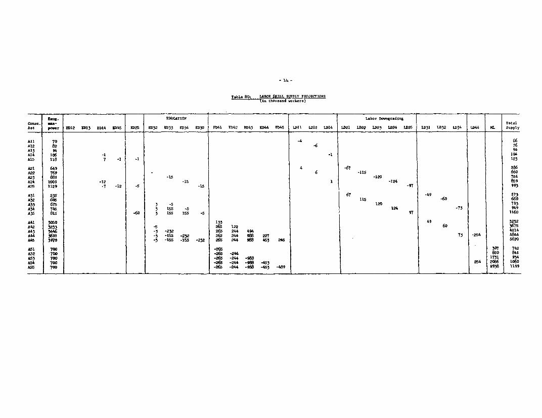
Table 80s LABOR SKILL SUPP2.Y PRDJECTIONSinthou...nd vor~kers)

Emos- *£EDUCATION Labor Dovograd ingCoat. ma-

TotalAst power £D12 £D153 D14 £D15 LD25 £D32 D33 1£D34 ED35 £1D41 £D42 1D43 1D44 E145 LD1L L_12 LD14 LD21 ,LD22 LD23 LD24 LD25 LD31 LD32 LD34 LD44 ML Supply

All 70 -4 66A12 82

-6 76A13 94

9A14 106 -1 -1 104AL5 118 7 -I -1

123A21 649

4 -67 586An1 769 6 -115 660A23 889 -15 -120 754A24 1009 -12 -15 1 -124 859A25 1129 -T -12 -5 -15 -97 993

A31 535 67 -49 673A32 605

11.5 -60 660A33 675 3 -5 1.20 793A34 745- 3 155 -5 124 -73 194A35 815 -60 3 155 15 -5 97 1160M41 3060 133 49 3232A42 3233 -5 265 1.22

60 3675M43 3446 -3 -232 265 244 494 4214A44 3691 -3 -155 -232 265 244 988 227

73 -254 4844AS 3970 -3 -155 -155 -232 265 244 988 453 245 5620

A51 700 -265 307 742A52 700 -265 -244 650 841653 700

-265 -244 -988 1731 934A54 700 -265 -244 -968 -453

254 2056 1060A55 700 -265 -244 -986 -453 -489 2938 1199

- 15 -

14.16 In 1972, the education system in Turkey has excess capacity of pro-fessionals, and shortage of skilled urban labor and middle-school level ad-ministrators. During the projection period, professionals will be downgradedto employments requiring a lower skill level and urban unskilled and sktlledlabor will be educated and promoted to higher skills. During 1972-87, educa-tion is given to nearly 3 million personi; in excess of what is provided bythe existing education system, and mostly to unskilled urban labor (2.4 million).

14.17 Changes in the skill composition of the labor force over the periodare significant, as can be expected in a fast growing and modernizing economy.The decrease in the share of professionals (skill 2) indicates an adaptationof the education system to the requirements of the growth pattern during theprojection period. The share of unskilled agricultural labor force in totallabor force decreases drastically from 68.3% in 1972 to 54.6% in 1987, how-ever, less fast than expected in the Government strategy (38% in 1987).

Table 81: COMPOSITION OF SKILLED LABOR FORCE

Skill 1972 1987

1. Scientists, engineers, doctors, professors 1.3 1.42. Other technical and professional 11.4 10.93. Administrative and clerical 10.0 12.84. Skilled and semiskilled urban 62.3 61.75. Unskilled urban 15.0 13.2

Total 100.0 100.0

14.18 Balance of Payments and Foreign Trade (Table 82). The programmingmodel is not designed to focus particularly on this problem. Availability offoreign exchange is specified exogenously, and the model can choose betweenimport substitution or five categories of exports. With the present coststructure of Turkey, a maximization of the GDP in the terminal year leads toa very rapid import substitution and to export growth only in the agriculturalsector. A 6% upper limit has been imposed to long-term growth of agriculturalexports, and a 10% lower limit to tourism exports. These limits prove to bebinding during the whole projection period. Manufacturing exports grow at10.7% per year and total exports at 7.7% per year, or slower than in the long-term strategy (10.1%). In absence of a constraint describing the effect ofthe entry of Turkey in the EEC, the optimization favors import substitutionduring the first time period and a more rapid trade growth of non-competitiveimports and exports in the later periods. Joining the EEC will lead to moreimports of goods which Turkey could produce at a competitive cost in the long-term, particularly of consumer goods and intermediate raw material. In thestructure of the planning model, it translates into more "non-competitve"goods. A sensitivity analysis describing the effect of this structuralchange has been carried out in the following section (paragraphs 28-29).

- 16 -

Table 82: Foreign exchange projections (Basic Case)

Unit: billions i972 TL

Year 1972 1975 1978 1981 1984 1987 AverageAnnual GrowthActivity Rate, 1972-1987

Non-competingimports LJ 14.4 20.5 26.5 33.9 43.1 53.4 9.2

Ml AgricultureIt. importa .4 - - - - - -

M2t Ydnngimports .3 .5 .7 1.1 1.6 2.4 14.9

M Manufacturing3,t. imports 10.3 7.8 7.1 3.3 .4 - -

Total imports 25.4 28.8 34.3 38.3 45.1 55.8 5.4

Z, Agrieulture.L,t. export8 8.o 9.5 11.3 13.5 16.1 19.2 6.o

Z2,t. Mining exports .5 .5 .5 .5 .5 .5 -Z3,t- Manufacturing

exports 3.3 3.3 3.3 5.1 8.7 15.1 10.7Z4,t. Freight & shipping

exports .2 .2 .2 .2 .2 .2 -Z5,t. Tourism 1.5 2.0 2.7 3.5 4.7 6.3 10.0

Total exports 13.5 15.5 18.0 22.8 30.3 4l.3 7.7

Invidsibles &net foreign loans 11.9 13.3 16.3 15.5 14.8 14.5 1.3of which: net foreign loans 8.6 2.8 1.7 .t - -

net factor services 9.0 13.3 17.6 17.9 18.2 18.1 16.0/ Imports of raw material and equipment goods for which Turkey will not become competitive in theprojection period.

- 17 -

14.19 Dual Variables. Associated with a programming model of this kind,there are dual variables, also referred to as shadow prices or efficiencyprices. These are of great interest and importance in linking "macro" plan-ning with project evaluation and the decentralized decision-making of multi-level planning. They reflect the shadow prices of scarce resources (such asforeign exchange, output, labor, and capacity) and other economic constraints(such as limits on the rate of growth of exports and the marginal propensityto save).

14.20 Shadow prices are most important in those situations where marketprices do not adequately reflect true economic scarcity either statically ordynamically. Typically, the market prices in LDC's are especially poor in-dicators for a number of reasons. Most importantly, if unskilled agriculturallabor is in surplus, its efficiency price is zero even though there is a po-sitive wage rate. This can lead to serious overvaluation of labor in projectswhich are valued using market prices and therefore choice of techniques withtoo low labor-capital'ratios. Overinvestment in physical capital not onlywill lead to inefficiency in the use of scarce resources, but could also leadto a worsening of the distribution of income against the unskilled workerswho make up the bulk of the labor force. Finally, using market prices thereis no obvious way to take account of changes in relative prices, a problemautomatically taken care of when shadow prices are used. The analysis ofdual variables associated with the programming model has not been carried outvery far. Tables 8 and 9 indicate the shadow prices associated with sectoralactivities and skill levels. These shaclow prices have been normalized by theshadow price of consumption in each time period, to avoid the trend declineover time of shadow prices which reflect the decreasing marginal productivityin terms of the maximized function.

14.21 The shadow prices of sectoral activities are the value of one billionof output of a sector compared to one billion of output of consumption in aperfect market economy and reflect the distortion of the present price system.They would all equal one in a perfectly competitive market. Utilities, trans-port and services are relatively high cost sectors, and the distortion in thecost structure seems to remain about the same over the whole period (Table 83).

14.22 As shown in Table 84, shadow wages of skilled labor 1 to 3 increaseover time, while shadow wages of skilled and unskilled urban labor declineover time. This indicates only the increasing scarcity of high skilled man-power in a fast growing and modernizing economy. The equality of shadowwages in skills 1 to 4 in the early years of the projection indicates onlysome skill downgrading in skills 1 to 3 which puts the efficiency price oflabor in these groups at the level of the lower skill. Although Turkey isconsidered in the programming model as a labor surplus economy for unskilledlabor force in agriculture, which supplies urban unskilled labor (skill 5)with migrants, the shadow wage of skill 5 is not zero, because of the costof these migrations to the economy (TL 2900 per man and per year, or a littleless than the normalized shadow wage of skill 5).

- 18 -

Table 83: Dual variables for material balances (Bit), foreignexchaange balances (Ct) and consumption (ACt)

(Units: 1972 TL per unit of good i, normalized bydual variable for consumption in year t)

(Basic case)

Year 1975 1987

Sector i

1. Agriculture .751 .783

2. Mining .991 1.210

3. Manufacturing .807 .839

4. Utilities 2.320 2.431

5. Construction *520 .540

6. Commerce .349 *340

7. Transportation 1.154 1.219

8. Services 1.437 1.328

Foreign exchangelJ .807 .863

Dual variable forconsumption (interms of maximaxnd) .755 1.422

11 The shadow price of foreign exchange is always equal to the shadowprice in the manufac'turing sector, which forms the bulk of internationallytraded goods, but in the terminal year. This indicates that there seemsto be no premium 'on foreign exchange, or 'that the conventional price offoreign exchange equals its shadow price. The difference in the terminalyear reflects terminal conditions problem. The shadow interest rate onforeign capital between 1975 and 1984 averages 11.5% per year.

- 19 -

Table 84: DUAL VARIABLES FOR LABOR BALANCES (Ast)

(Units: 1972 TL per man-year ofskill level s, normalized by dualvariable for consumption in year t)

Year 1975 1987

Skill s

1. Scientists, engineers,doctors, professors 4888 11974

2. Other technical andprofessional 4888 7458

3. Administrative andclerical 4888 7458

4. Skilled and semi-skilled urban 4888 4190

5. Unskilled urban 4368 3611

- 20 -

14.23 Larger differences betwoen shadow wages of low and higher skills donot indicate a deterioration of the income distribution. Shadow wages arecalculated independently from all sorts of considerations which determinethe level of real wages, such as minimum salary legislation and the bargainingpower of trade uinions. The changes in the skill composition of the labor forcelead to nearly no increase in the average shadow wage which changes from TL4814 in 1972 to TL 4993 in 1987. With skilled labor force increasing at 4.6%per year and the average shadow wage increasing at 0.3% per year, skilledlabor income increases at 4.9% per year or less fast than consumption (6.8%).

Alternative Growth Patterns

14.24 Modifications to the assumptions made in the basic case have beenintroduced one at a time. Six alternative solutions have been exploree, andare described in Table 85. Although some of the modifications introduced arerather extreme, they do not have a large impact on the pace of growth of theTurkish economy. Thus, the yearly growth rate of GDP always remains between7.0% and 7.6%. This result is typical o.f linear programming models; relaxingone constraint allows to increase growth as long as another constraint doesnot become binding. 1/ While overall growth is not very sensitive to thevarious alternatives, some particular variables are. The comparison of anumber of alternatives with the basic case is summarized below and in Table 86.

14.25 An employment oriented economy. The trade-off between a maximumgrowth and a maximum employment strategy in the long-term is described incase 1 of Table 86. To avoid that the model creates excess supply of outputin labor intensive sectors for the sake of employment creation, final outputhas been constrained to equal demand in 1987. In the programming model, un-skilled agricultural labor force is considered in surplus, and constitutesthe source of rural urban migrations to create the skilled and unskilledurban employment required by the pace and pattern of growth. As a consequenceof these characteristics, maximizing employment leads the model to emphasizegrowth of industry and services at the expense of agriculture. Industrialoutput grows faster than in the basic case (9.1% compared to 8.6% as servicesoutput (7.4% compared to 7%) while agricultural output grows falls to 2.4%(compared to 5.6Z). The overall economy grows only slightly more slowly(7.0% compared to 7.2%), as well as investment, consumption and savings. Thepattern of investment is more oriented,towards services (55% of total invest-ment compared to 47%) at the expense of agriculture (7% compared to 14%).More growth in the modern sector leads to uore exports, especially in indus-trial exports (20% compared to 10.7%) and to more imports growth (10.3% com-pared to 5.4%), a substantial amount of agricultural imports being due to thelow agricultural growth. As expected, this employment strategy leads to a

1/ It would be easy to build cases where the growth rate "blows up" byrelaxing several constraints. Such cases have not been envisaged be-cause they were found unrealistic.

- 21 -

Table 85: ALTERNATIVE SOLUTIONS

No. Name Characteristics

1. Employment-oriented economy Maximization of employment (insteadof GDP) - oversupply of materialgoods at the end of the projectionis not allowed.

2. Labor surplus economy No labor constraints for all skilllevels.

3. Less domestic savings Marginal propensity to save (MPS)= .24

4. More domestic savings MPS=- .30

5. More dependence from Increased net foreign capital borrowing.foreign capital

6. EEC membership Less competitive economy (in the sense ofthe model): more non-competitive importsin consumption and raw material.

- 22 -

Table 86: Sensitivity Analysis

163-lY72 1972-1987Basic case Max.employ. Labor surplus MPS=o24 MPS=e30 liore borrowing EEC entry Turkish Dev.

Yearly 5owth Rates (%) (1) _ (2) (3) (4) (5) (F) Strategy

G market prices) 6.6 7.2 7.0 7.5 7.0 7.6 7.5 7.2 8.7Consumption 6.o 6.6 6.4 6.9 6.5 6.7 6.8 6.6 7.5Domestic Savings 10.2 10.2 9,9 10.5 9.5 11.6 1m5 I.2 11.8

Investment 9.8 8.5 8.33 8.8 7o9 9.8 8.9 8.5 11.2MPS L .22 .26 .26 .26 .24 .30 .26 .26 *3$5

Total imports 6.5 5.4 10.3 5.1 4.9 6.4 5.6 9.2 7.6Non-competitive

imports n.a. 9.2 8.3 8.8 8.9 10.2 9.4 13.2 r.a.

Total exports 7.0 7.7 14.0 7e3 7.1 9.1 7.9 12.6 10.1

Industrial exports 11.8 10,7 20.0 9,3 8.7 14.0 11,0 19e2 17,9

Total urbanemployment 5.8l 5.0 6 2 n.a. 4k7 5.6 5.3 5.0 5.2

Volume of migrationL.in 1987 (milions) 2.9 4.7 n.a. 2.5 3.8 3.14 2.9 n,a.

Agriculturallabor force .9 ' I1 n.a. 1.2 .5 .7 .9 - .6

Growth of outputAgriculture 3 .6L 5.6 2.4 5.8 5.5 5.8 5.6 5.4 5.1Industry 10.2 A 8.6 9.1 8.8 8.3 9.1 8.9 8.4 11.3

Services 7.2 7.0 7.4 7.2 6.8 7.5 7.3 7.2 8.9Total 6.6 7.3 7.3 7.6 7.1 7.9 7.6 7.3 9.3

Structure ofinvestment (% oftotal during period)

Agriculture 13 15 7 14 13 12 12 15 10Industry 35 38 38 37 41 41 42 37 48Services 32 47 55 49 146 47 146 48 42

GDP per capita in 1987,in 1972 US$ 119 776 831 776 848 828 794 996 j

1. Marginal propensity to save during 1972-19812. Accumulated migrations daring 1972-1987 for urban employment creation3. 1965-19704. Value added at factor cost5 Assumting a populatLon of 52.8 millions in 1987

- 23 -

much faster growth of urban employment (6.2% compared to 5.0%) in all skilllabors, including labor employed in new education activities which increasesfrom about 600,000 in the basic case to 1.7 million; and to a slight decreaseof agricultural labor force during the period, and to the migration of abouttwo million people more to the cities.

14.26 Compared to the Government long term strategy, it leads to a betteremployment situation, a lower per capita income but obtained with a less im-portant savings effort, and more emphasis on the services sector, a betterincome distribution within the urban area, but a deterioration in the relativeincome of the agricultural sector, unless a system of financial transfers isset up at the same time.

14.27 An economy without labor constraints. Assuming that growth is inno way constrained by skilled labor shortages, as the government long planstrategy and third plan projections do, leads to a faster economic growth thanin the basic case in all sectors. The difference is more important in theforeign sector, where exports and imports grow more slowly and the pattern ofimports is changed, with immediate total imports substitution in the manu-facturing sector and gradual import substitution in imports of agriculturalgoods, or the reverse situation from the basic case. This reflects a de-crease in the profitability of agriculture once skilled labor is also insurplus (Table 86, case 2).

14.28 Changes in the savings effort. The marginal ratio of.domesticsavings has been 26% during the First Plan and 13% during the Second Plan andis expected to increase to 38% during the Third Plan, and to 35% during thenext 22 years. Variations in the marginal savings rate affect significantlythe pace of growth of the economy, and the employment level, and to a lesserextent, the growth pattern. A variation of the marginal savings rate between26% and 30% increases the yearly growth rate of GDP from 7% to 7.6%, of invest-ment from 9.5% to 11.6%, of imports from 4.9% to 6.4%, and of exports from 7.1%to 9.1% with a particularly faster growth in industrial exports (14% insteadof 8.7%). In the employment sector, urban employment increases faster bynearly 1% per year, and more than 1 million more peasants migrate to work inthe cities. Growth increases in all sectors, but particularly in industryand services, and the investment pattern gives slightly more emphasis toservices at the expense of agriculture (Table 86, cases 3 and 4).

14.29 Relying more on foreign savings to sustain a fast pace of growthis equivalent to a harder savings effort in many respects. Assuming thatTurkey borrows net TL 17.8 billion more than in the basic case (which isequivalent to 50 million US$ of 1972 per year), GDP growth increases from7.2% to 7.5%, only in the industry and service sectors and urban employmentgrowth increases by .3% to 5.3% (Table 86, case 5). Reaching a faster growththrough more savings or more borrowing seems to have the same effect on thepattern of growth, and on the level of employment.

14.30 A more open economy. In the basic case, imports of intermediate andfinal goods have been classified into competitive and non-competitive, compet-itive imports being defined as imports of goods which could be produced at a

- 24 -

competitive cost in the long-term. The list of competitive imports preparedby Mr. Blitzer and Mr. C. Cetin (SPO) in 1970 served as a basis for thisclassification. The entry of Turkey into the EEC may create a situation inwhich Turkey will import more goods for which it will be competitive in thelong-term, but is not at present, or for which Turkey is competitive but con-sumers have a preference. To account for this possibility, the 1972 transactionmatrix and the input output and capital coefficients matrix, have been revised,with the assumption that more imports than in the basic case are non-competitive,mostly in the manufacturing sector (50% more in intermediate goods and 40%more in investment goods and consumer goods). These modifications leave thepace of growth and employment level unchanged, but modify the growth patternancl external sector (Table 86, case 7). Slightly more emphasis is given toinvestment in the services sectors, which grow faster while industry growsslightly more slowly.

14.31 The external sector presents a substantially different pattern.Imports grow faster (9.2% compared to 5.4%) since import substitution islimited to a narrower field. Exports increase also faster, (12.6% comparedto 7.7%), essentially due to a faster growth of manufacturing exports (19.2%per year instead of 10.7%). Although the disaggregation of the model doesnot enable to answer the problem of comparative advantage, this alternativecorresponds probably to a development strategy where Turkey speCializes inthe production of manufactured products in which it has a comparative advan-tage and where exports can increase fast.

ANNEX AlPage 1

Data Base for the Linear Programming Model

1. A detailed analysis of the data base for the programm:lng model isavailable in previous writings. 1/ This note is a brief description of themethod by which this data base has been updated during the basic economicmission.

Current Account Input-Output Coefficients (Tables Al, A2, A3)

2. The estimation of these coefficients is based on the 1967 input-output study done by the SPO, and the modifications to this table done forthe preparation of the Third Plan. These modifications account for techno-logical changes which have taken place during 1967 and 1972, and also forthe 1970 devaluation which raises the non-competitive import coefficientsand the imported part of the technical coefficients (competitive imports). 2/

3. A detailed analysis of the 1972 custom statistics enabled us toclassify import between competitive and non-competitive, and between consump-tion, intermediate deliveries, and investment. The list of competitive im-ports prepared by Mr. Blitzer and Mr. H. Cetin (SPO) in 1970 proved to be ex-tensive enough not to have to be revised.

4. The 37 sectors coefficient matrix was then aggregated into 8 sectors,using the 1967 transaction matrix values as weights to average the coefficients.Some coefficients were then modified to account for further technologicalchanges during 1972-1987, essentially in utilities, commerce and agriculture.

Capital Coefficients (Table A4)

5. The capital coefficients matrix was revised from new Turkish sourcesof information. 3/ Total ICOR was raised in agriculture, mining, utilities andlowered in construction, commerce and services. The ICOR were then brokendown into sectors of origin following the previous methodology 4/ and using the1967 input output analysis. The student-investment ratios were updated toaccount for the price changes between 1963 and 1972.

Export Coefficient (Tables A5, A6, A7)

6. The only modification to the export delivery coefficients consistedof shifting 10% of the origin of tourism exports from services to agriculture.Long term upper limits on export growth rates were increased to 6% for agri-culture and 20% for manufacturing on the basis of mission analysis of exportprospects.

1/ R. Blitzer, ibid. Appendix: Numerical data for PPM.2/ For a detailed explanation of the technological changes, see "Explanatory

note of the 1967 I-0 study for the use in the TFYP model, internationalcolloquium on the TFYP model, SPO (February 28-29, 1972).

3/ Sevin Yayin and Nuran Uras, TFYP. Marjinal sermaye - uretim iliskilleri,SPO (1971).

4/ C. Blitzer, ibid.

ANNEX AlPage 2

Incremental Consumption Coefficients (Table A8)

7. These coefficients were revised on the basis of the 1967-1972performance.

Urban Transformation Cost (Table A9)

8. This cost was revised on the basis of a study carried out by thePlanning Office of the Ministry of Reconstruction and Resettlement, and hasbeen estimated to TL 2,900 in 1972 prices.

Labor Input and Labor Force Projections (Tables AIO, All, A12, A13, A14)

9. The procedure used to prepare exogenous projections of labor forcehas not been changed, but projections are now based on the results of the1970 census, from which estimates of employment and skill for 1972 have beenderived. Projections of productivity changes have been modified according towork carried out in the SPO by Mr. Yigit Alemdar and of the mission analysis.The labor input norms for production by sector and by skill (lts,j) have beenrecalculated accordingly.

10. On the basis of the new estimates, labor balances by skill in 1972indicate significant deficits in skills 3 and 4 made of clerical workers andadministrative with about 3 years of high school, and of middle school educatedtaclricians. There seems to be excess supply of professionals, and of unskilledurban labor, indicative of urban underemployment (Table A14).

Material and Foreign Exchange Balances (Tables A15, A16)

11. The constants of the material balances constraints are calculatedfrom Table A3 and from population projections prepared by the Bank and in-cluded in Table All.

12. The constants of the foreign exchange constrains are made of exogenousprojections of net factor income, net changes in reserves, and net capital in-flows. These constants have been determined in the basic case solution of abalance of payments analysis with a two-gaps model (see Annex II B). Workers'remittances have been assumed to increase from $900 million in 1972 to $1,300million in 1977, then to $1,700 million in 1987 in constant 1972 prices.Profits increase 5% per year from $35 million in 1972, interest increases10% per year on average from $62 million in 1972. Taking into account theTurkish strategy of less dependence from foreign savings, net capital inflowsdecrease from $275 million in 1972 to $247 million in 1987 in dollars of 1972out of which net official capital decreases from $177 million in 1972 to $70million in 1987. Net reserves, calculated as a residual item in the balanceof payments equilibrium, change as indicated in Table A16.

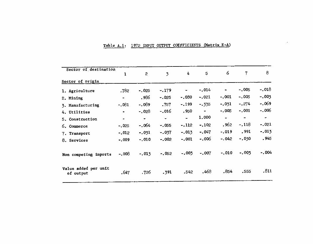
Table A.l: 1972 IN'PUT OUTPUT COEFFICIENTS (Matrix E-A)

Sector of. destination

1 2 3 4 5 6 7 8

Sector of origin

1. Agriculture .782 -.025 -.179 - -.014 - -.005 -.018

2. Mining - .986 -.025 -.080 -.021 -.001 -.005 -.003

3. Manufacturing -.081 -.089 .757 -.199 -. 335 -.031 -.274 -.069

4. Utilities - -.028 -.016 .950 - -.005 -.001 -.006

5. Construction - - - - 1.000 - - -

6. Commerce -.025 -.064 -.055 -.112 -.102 .962 -.118 -.021

7. Transport -.012 -.031 -.037 -.013 -.047 -.019 .991 -.013

8. Services -.009 -.010 -.002 -.001 -.006 -.042 -.030 .945

Non competing imports -.008 -.013 -.052 --003 -.007 -.010 -.003 -.004

Value added per unitof output .647 .726 .391 .542 .468 .854 .555 .811

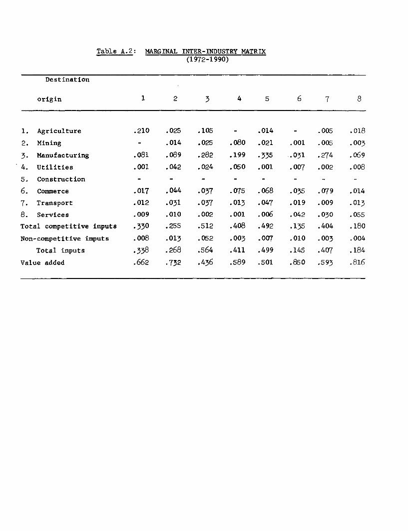
Table A.2: MARGINAL INTER-INDUSTRY MATRIX(1972-1990)

Destination

origin 1 2 3 4 5 6 7 8

1. Agriculture .210 .025 .105 - .014 - .005 .018

2. Mining - .014 .025 .080 .021 .001 .005 .003

3. Manufacturing .081 .089 .282 .199 .335 .031 .274 .069

4. Utilities .001 .042 .024 .050 .001 .007 .002 .008

5. Construction - - - - - - - _

6. Commerce .017 .044 .037 .075 .068 .035 .079 .014

7. Transport .012 .031 .037 .013 .047 .019 .009 .013

8. Services .009 .010 .002 .001 .006 .042 .030 .055

Total competitive inputs .330 .255 .512 .408 .492 .135 .404 .180

Non-competitive imputs .008 .013 .052 .003 .007 .010 .003 .004

Total inputs .338 .268 .564 .411 .499 .145 .407 .184

Value added .662 .732 .436 .589 .501 .850 .593 .816

Table A.3: 1972 TRANSACTION MATRIX(1972 billions T.L.)

Deliveries Intermediate Total

origin deliveries Consumption Investment Exports demand Imports Output

1. Agriculture 40.9 36.4 - 6.4 83.7 .4 83-3

2. Mining 4.4 1.2 .3 5.9 .3 5.6

3. Manufacturing 59.1 57.7 7.6 3.0 127.4 10.3 117.1

4. Utilities 2.9 3.7 - - 6.6 - 6.6

5. Construction - - 27.1 _ 27.1 _ 27.1

6. Commerce 17.8 7.5 .8 1.2 27-3 - 27.3

7. Transport 8.4 14.3 .2 1.2 24.1 _ 24.1

8. Services 6.5 55.2 - 1.4 63.1 63.1

Non-competing imports 7.1 .8 6.5 - 14.41' 14.4-1 -

Total 147.1 176.8 42.2 13.5 379. 1/ 25.41' 354.2

l/ Including import taxes

Table A.4: CAPITAL COEFFICIENT MATRIX

Destination

origin 1 2 3 4 5 6 7 8 9 10 11

3. Manufacturing .47 .88 .32 .51 .10 .o6 .80 .07 .20 .13 .075. Construction .85 .13 .30 3.35 - .13 1.00 3.30 .52 .70 .836. Commerce .10 .30 .08 .40 .02 .04 .21 .03 .06 .04 .027. Transport .03 .18 .02 .11 .01 .01 .o6 .01 .02 .01 .02

Non-competing imports .25 1.28 .28 2.33 .10 .16 .68 .11 .20 .12 .o6

ICOR 1.70 2.67 1.00 6.70 .23 .40 2.75 3.52 1.00 1.00 1.00

Student-investmentratio 35.5 56.0 153.6

Table A.5: EXPORT DELIVERY COEFFICIENTS (zi )

exportactivity, j Agricul- Manufac- Freight

tural Mining turing andsector of goods goods goods Shipping Tourismorigin, i

1. Agriculture .769 - - - .100

2. Mining - .683 - --

3. Manufacturing - .796 - .251

6. Commerce .089 .131 .076 .032 .o76

7. Transport .073 .125 .056 .888 .099

8. Services o069 .061 .072 .080 .474

Total 1.000 1.000 1.000 1.000 1.000

Table A.6: EXPORTS IN 1972

(billion TL)

Agricul- Manufac- Freighttural Mining turing andgoods goods goods Shipping Tourism Total

Agriculture 6.2 - - - .2 6.4

Mining - .3 _ - - .3

Manufacturing - - 2.6 - .4 3.0

Commerce .7 .1 *3 - .1 1.2

Transport .6 .1 .2 .2 .1 1.2

Services .5 - .2 . .7 1.4

Total 8.0 .5 3.3 .2 1.5 13.5

Table A.7:UPPER LIMITS ON EXPORT GROWTH RATES

3Export Activity Upper growth rate (ei) (1 + ei)

1. Agriculture 6% 1.191

2. Mining 15% 1.521

3. Manufacturing 20% 1.728

4. Shipping, freight 10% 1.351

5. Tourism 20% 1.728

Table.A.i8: INCREMENTAL CONSUMPTION COEFFICIENTS

Agriculture 12.2

Mining .4

Manufacturing 45.0

Utilities 2.0

Cormerce 5.O

Transport 10.0

Services 25.0

Non-competing imports , .4

lO.0

Table A.9: Urban Transformation Costs (Fi)

The Planning Office of the Ministry of Reconstruction and Development

has estimated that the costs of absorbing the additional population of

Ankara would be approximately TL 25,859 per capita during the Third Plan,

broken down as follows:

Destination TL/capita

1. Drinking water 1,240

2. Sewage 417

3. Electricity 220

4. Roads 1,609

5. Markets, car parks, etc. 7,320

6. Accomodation 10,050

7. Transport 5 ,000

8. Plans and designs 3

TOTAL 25,859

Assuming that a) expenditure on 1, 2, 3 and 5 is current expenditure

b) expenditure on 4, 6 and 7 has to be repeated every 20 years, and on S

every 40 years, the annual expenditure per capita comes to TL 2,900,

broken down intoTL

Utilities 330

Transport 330

Services 2,240

2,900

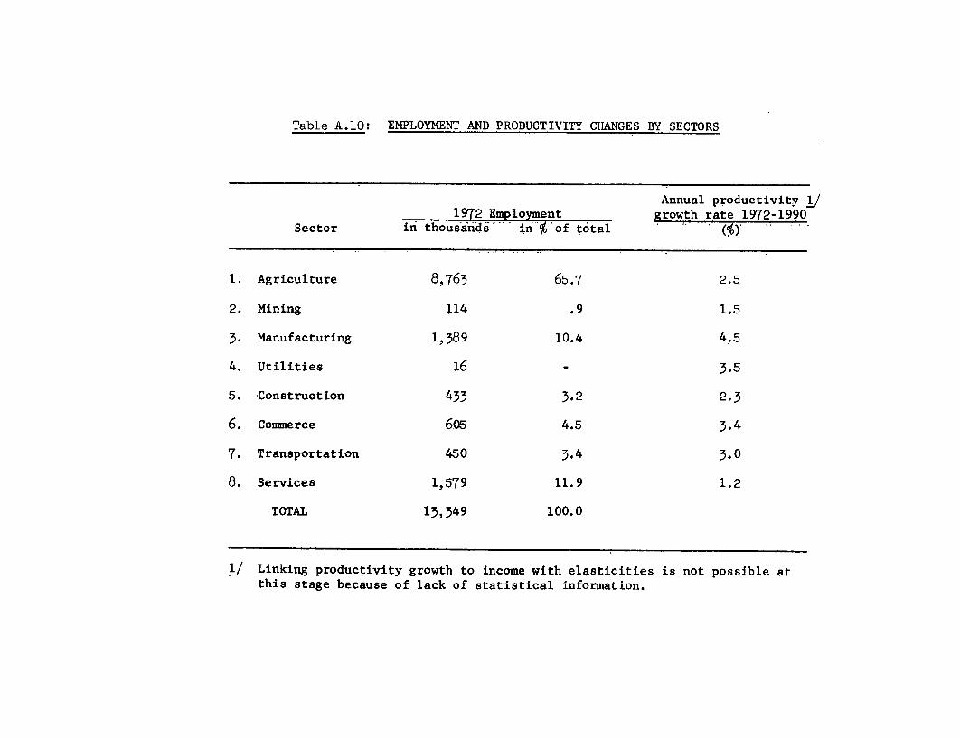
Table A.10: EMPLOYMENT AND PRODUCTIVITY CHANGES BY SECTORS

Annual productivity /1972 Employment growth rate 1972-1990

Sector in thousarnd- "' in-%'of total (%)

1. Agriculture 8,763 65.7 2.5

2. Mining 114 .9 1.5

3. Manufacturing 1,389 10.4 4.5

4. Utilities 16 - 3.5

5. Construction 433 3.2 2.3

6. Commerce 605 4.5 3.4

7. Transportation 450 3.4 3.0

8. Services 1, 579 11.9 1.2

TOTAL 13,349 100.0

S/ Linking productivity growth to income with elasticities is not possible atthis stage because of lack of statistical information.

Table A.ll: 13xgenous Projections of Labor ForceIn thousands (yearl growth rate)

Non-agrIcultural andSkill 1 2 3 4 5 6 agricultural skilled Total Total

labor force labor force Population1960 30 167 289 1591 462 9091 2539 11630 27755

(1.3) (8.3) (l.o) (4.2) (-1.8) (1.4) (3.1) (1.8) (2.5)1965 32 249 303 1959 421 9723 2964 12687 31391

(9.8) (12.5) (6.7) (6.6) (8.3) (--) (714) (1.9) (2.6)1970 51 449 419 2691 628 9723 4238. 13961 35667

(6.7) (8.5) (5.3) (1.1) (__) (2.5) (2.5) (2.5) (2.6)1972 58 529 465 2894 700 10020 4646 134666 37200

(6.5) (7.1) (4.8) (1.8) (-_) (2.5) (2.5) (2.5) (2.6)1975 70 649 535 3050 700 10792 5004 15796 40177

(5.4) (5.8) (4.4) (2.0) (__) (2.5) (2.5) (2.5) (2.5)1978 82 769 605 3233 700 11622 5389 17011 43266

(4.7) (4.9) (3.7) (2.1) (__) (2.5) (2.5) (2.5) (2.4)1981 94- 889 675 3446 700 12517 5804 18321 46457

(4.0) (4.3) (3.2) (2.3) (_-) (2.5) (2.5) (2.5) (2.2)1984 106 1009 745 3691 700 13481 6251 19732 49590

(3.7) (3.8) (3.o) (2.) (--) (2.5) (2.5) (2.5) (2.1)1987 118 1129 815 3970 700 14519 6732 21251 52780

(3.3) (3.4) (2.8) (2.6) (_) (2.5) (2.5) (2.5) (2.0)1990 130 1249 885 -42 87 700 15638 7251 22889 56010

Table A.1 SECTORAL EMPLOYMENT COEFFICIENTS(thousand men yeair/Billion TL output in 1972 prices)

Annual Productivity1972 1975 1978 1981 1984 1987 1990 growth (%)

Agriculture .72 .67 .62 .57 .54 .50 .46 2.5

Mining 20.4 19.3 18.5 17.7 16.9 16.1 15.4 1.5

Manufacturing 11.9 10Q4 9.1 8.0 7.0 6.2 5.4 4.5

Utilities 2.4 2.2 2.0 1.8 1.6 1.4 1.3 3.5

Construction 16.0 15.0 14.0 134 12.2 11.4 10.6 2.3

Commerce 22.2 20.0 18.1 16.4 14.8 13.4 12.1 3.4

Transport 18.7 17.1 15.7 14.3 13.1 12.0 11.0 3.0

Services 25.0 ?4.1 23.3 22.,5 21.7 20.9 20.2 1.2

table A.131 IABOR COIYTICllNS NATRICES (1t

Skill 1 2 5 4 1 2 3 4 1 2 3 4 5

Sector j

1 .047 .045 .231 .397 - .72 .037 .035 .183 314 - .57 .030 .029 .148 .264 - .462 .245 .408 1.265 7.650 10.832 20.4 .212 .354 1.09? 6.638 9.399 17.7 .18S .308 .gs5 5.775 8.177 15.43 .095 .296 .750 10.590 .167 11.9 *o66 .201 .504 7.124 .112 8.0 .040 .135 .340 s 4.S .076 s.44 .055 .137 .372 1.514 .322 2.4 .041 .103 .279 1.136 .241 1.8 .030 .074 .202 .820 .174 1.35 .080 .416 .64o 7.168 7.696 16.0 .066 .341 .524 s.869 6.301 13.1 .053 .276 .424 4.749 5.099 10.66 .o67 .422 6.660 14.052 .999 22.2 .049 .312 4.920 10.381 .738 16.4 .036 .230 3.630 7.65s .545 12.17 .056 .355 3.946 14.006 .337 18.7 .042 .272 3.017 10.711 .257 14.3 .033 .209 2.321 8.239 .198 11.08 .6so 5.625 4.950 11.400 2.375 25.0 .s8s s.063 4.485 10.260 2.138 22.5 .525 4.545 4.000 9.211 1.919 20.2

1l ~~~~ ~~1 14 .4s.1 a .

1 .045 .042 .215 .369 - .67 .035 .033 .173 .297 - .542 .2 2 .386 1.197 7.238 10.248 19.3 .203 .338 1.048 6.338 8.974 16.93 ,284 .260 .655 9.256 .146 10.4 .os6 .175 .441 6.929 .098 7.04 .061 .125 .341 1.388 .295 2.2 .037 .091 .248 1.010 .214 1.6

.075 .390 .600 6.720 7.215 15.0 .061 .317 .488 5.466 5.868 12.2.060 .380 6.0o0 12.660 .900 20.0 .044 .281 4.440 9. 68 .666 14.8

7 .021 .325 3.608 12.808 .308 17.1 .039 .249 2.764 9.812 .236 13.11q .627 5.423 4.772 10.990 2.290 24.1 .564 4.882 4.297 9.895 2.062 21.7

12 .2 1s.. as

I ..041 .038 .199 .342 - .62 .033 .031 .160 .276 . .502 .222 .370 1.147 6.938 9.824 18.5 .193 .322 .998 6.038 8.549 16.13 .073 .228 .573 8,098 .128 9.1 .0o0 .155 .390 s,s6 ,086 6.a4 .046 .114 .310 1.262 .268 2.0 032 .080 .217 .88, .188 1.45 .070 .364 .560 6.272 6.734 14.0 .057 .296 .456 5.107 5.483 11.46 .054 .344 5.430 11.487 .815 18.1 .040 .255 4.020 8.482 .603 13.41 .047 .298 3.313 11.759 .283 15.7 .036 .228 2.532 8.988 .216 12.0a .606 5.243 4.613 10.625 2.214 23.3 .543 4.703 4.138 9.530 1.986 20.9

Table Al4l LABOR BALANCES IN 1972(in 'thousand persons)

_ .......... , .~~~~~~~~~~~~~~~: .

'Skill class L -. lV TX. Total8, 0 8, J-,:0

1. University level 58 63 - 5

2. Other technical, professional 529 - 426 103

3. Administrative, clierical 465 - 722 -'257

4. 'Skilled and semi-skilled urban 2,894 -2,959 - 65

5. Unskilled Ourban 700 - 476 224

'Total 4,646 -4,646 0

Table A.15: RIGHT HAND CONSTANTS FOR MATERIAL BALANCES: P tci -(net output)?

Year1972 1975 1978 1981 10984 1987 1990

Sector

1 - 6.0 - 3.1 - .1 3.0 6.1 9.3 12.4

2 - .1 .2 .3 .4 .5 .6

3 -. 3 4.4 9.2 14.2 19.0 23.9 28.9

4 - .3 .6 .9 1.2 1.5 1.8

5 -27.1 -27.1 -27.1 -27.1 -27.1 -27.1 -27.1

6 - 2.0 - 1.4 -. 8 -. 2 .5 1.1 1.8

7 - 1.4 -. 3 1.0 2.2 3.3 4.6 5.8

8 - 1.4 3.0 7.7 12.4 17.0 21.7 26.5

Table A.16: RIGHT HAND SIDE CONSTANTS FOR FOREIGN EXCHANGE CONSTRAINTS(in Billion 1972 TL)

1972 1975 1978 1981 1984 1987 1990

1972 Intermediate imports 7.1 7.1 7.1 7.1 7.1 7.1 7.1

plus P C° .8 .9 1.0 1.0 1.1 1.2 1.3t m

plus net increase inreserves 5,7 3.6 3.4 5.8 6.b 6.5 7.0

less net capit-al in tlow -8.6 - - 5 4'2 -3.7 -3t5 -2.5

less net factor services -9.O -13.0 -15.2 -17.1 -17.3 -17. 5 -17.7

RHS -5.d -5.3 8.3 - 7.4 - 6.6 - 6.2 -3.8

p/ Includes short terimi capitai aid eii6rs aiid 'omissiobis

Table A.17 Skill Categories of Labor Force

Skill Definition

1. Scientists, engineers All university professors regardless of field,Professors. natural scientists, physicians, dentists, veter-

inarians, engineers and architects. In generalthe education level attained by this group corres-ponds to more than three years of higher education.

2. Technical and professional All other workers, except those already includedworkers. in skill level 1, included in the Turkish population

census as technical and professional workers. Themajority of this category are teachers. Alsoincluded are such diverse occupations as imams,lawyers, medical technicians and artists. The levelof educational achievement is in general equivalentto three years of university.

3. Managerial and clerical workers Those classified under this category in the Turkishpopulation census. The education level of thisgroup is roughly equivalent to three years oflycee (high school).

40 Skilled and semi-skilled workers Those whose jobs in general require the equivalentof a middle school education. This categoryincludes crEftsmen, production workers, drivers,police, and salesmen, among others.

5. Unskilled urban workers This group of occupations has little or no requi-rement for education above the primary level. Assuch, many of the new migrants into the urbanlabor force are engaged in work of this skilllevel. These occupations include miners, manualworkers, servants, dDormen, shoeshiners, andstreet peddlers.

6. Unskilled agricultural workers They form the bulk of the Turkish labor force.Although this group is primarily farmers, italso includes lumbermen, fishermen and hunters.In general the highest level of educationachieved is primary schooling.

ANNEX A2Page 1

Further Improvement of the Programming Model

1. The use of this prograiming model has been a first step towards abetter understanding of the alternative possible growth patterns of Turkeyand of the trade-offs between various policies.

2. A second step would consist of carrying further research to improvethis model. There are many directions of improvements, amongst which thefollowing can be indicated:

(1) Link of productivity growth and skill composition withincome in each sector: this would require data collec-tion on employment by sector and the estimation of in-come elasticities.

(2) Introduction of a public sector into the model, es-pecially with public investments, public savings, andthe analysis of the link between private savings andpersonal income.

(3) Further analysis of the changes overtime of industrialcompetitiveness in Turkey: this would require a compari-son of the cost of industrial production with the costof CIF imports and an appraisal of the future potentialchanges.

- 25 -

B. A Two-Gap Model for the Turkish Economy 1/

Objective of the Model

14.32 The main objective of this two-gap model is to estimate the foreigncapital requirements of the Turkish economy for 1973-87. The other objectivesare to measure the impact of inflation on domestic savings, foreign trade,and the requirement of foreign resources, and the impact of large inflows ofworkers' remittances on growth.

Description of the MIodel -

14.33 Like other models of this type, this one compares the ex ante for-eign exchange gap with domestic savings gap on the basis of a giver set oftarget growth rates in four major sectors of production (agriculture; industry;construction; services). Then, with the assumption that the dominant one ofthe two gaps will be filled by resources from abroad, the ex post identity ofthe two (I - S = M - X) is established within the framework of national accounts.

14.34 Unlike other models of this type, however, this one employs domesticand foreign prices as one of the determinants of the behavior of real economy,thus allowing for the room to test the impact of different policy decisionson such instruments as exchange rate or domestic money supply. Although fulldescription of the model will be presented in the Annex, a brief descriptionis presented below.

14.35 Simulation over some part of the observation period (1967-72) hasbeen conducted to test the predictive ability of the model, and the range ofprediction errors on all major economic indicators falls within the acceptablelimit (5% of the real value). The important endogenous variables are moneydemand, GNP deflator, effective terms of trade, private and public consumption,ICORs, imports of capital goods, raw materials, consumer goods and non-factorservices, net and gross foreign capital requirements. The exogenous variablesare money supply,3/ the growth rate of value-added in four major productionsectors (agriculture, industry, construction and services), exports, workers'remittances, and the official exchange rate.

14.36 Sensitivity analyses have been carried out to measure the trade-offsintroduced by changes in money supply growth, exchange rate, export growth,workers' remittances,-and the borrowing terms of foreign capital. Variablesof national accounts (GDP, GNP, sectoral value-added, investment, consumption,

1/ This model has been developed with the close cooperation of ComparativeAnalysis and Projections Division of the Bank, and particularly of Mr.Garcia dos Santos.

2/ See technical appendix for a detailed analysis.

3/ An attempt to project money supply growth on the basis of the variableswhich "explained" most of this growth in the past (Treasury borrowingfrom Central Bank, agricultural price supporting credit and foreignassets) has been abandoned (see technical appendix).

- 26 -

and exports and imports of goods and non-factor services) are estimated inconstant 1968 Turkish Lira while the components of balance of payments areestimated in current US dollars.

14.37 The domestic price changes are explained by the changes in thedemand for and the supply of money. Money demand, in turn, is explained byreal GDP and prices, and money supply is taken as a policy variable.

14.38 Starting from a set of target growth rates for the four major pro-ducing sectors, we determine the investment requirements through incrementalcapital output ratios (ICORs), which were estimated on the basis of pastrelationship between investment and value added growth rate. Private con-sumption, and therefore domestic savings, is explained by disposable incomeand prices whereas Government consumption is mainly explained by the levelof GDP. Three different functions have been specified for commodity imports.They all include effective terms of trade as an explanatory variable, measuredby an index representing the composite effect of the changes in custom dutyrate, domestic price, international price of imported goods, and the officialexchange rate. The other variables explaining the value of commodity importsare fixed investment and export plus workers' remittances for capital goods;value-added in industry for intermediate goods; and disposable income as wellas the rate of import substitution for consumer goods. Imports of non-factorservices are explained by a time trend.

14.39 The two ex ante gaps between investment - saving and import - exportsare equialized ex post through changes-in-stock; if the changes-in-stock reacha maximum or minimum allowed in a year, the rest of the adjustment comes fromprivate consumption and imports..

14.40 Gross foreign capital requirement equals the sum of the ex postresource gan in current dollars, foreign debt service payments, and the ex-pected profit transfers by foreign-owned firms. Foreign exchange availabilityis exogenous, and includes workers' remi-ttanices, official project and programassistance, TL grain imports under PL 480, NATO infrastructure and off-shorereceipts, import-s with waiver, and direct investment. Official capital in-flows are projected on the basis of existing loan commitments and expectedpipelines. If the foreign exchange requirements exceed their availability,the gap is filled first by drawing on the reserve holdings of the CentralBank until the reserve level reaches a minimum of three months' equivalentof imports, and then by an inflow of suppliers' credit. If foreign exchangeavailability exceeds the requirements, accumulation of reserves takes place.

Case 1 - Basic Case

A. Assumptions

14.41 The basic case has the following underlying assumptions on majorexogenous variables:

- 27 --

(a) The annual growth rates of value added at factor cost inagriculture, industry, construction, and the services sectorare 4%, 11%, 8%, and 8% respectively.

(b) Money supply increases at 17% per year (26% during theSecond Plan) during the Third Plan, and 14% per yearthereafter.

(c) Export grows by 25% in 1973, by 8% until the end of 1977,and grows at 9.3% per annum thereafter.

(d) Workers' remittances reach $900 million in 1973 and $1400million in 1977 (current dollars). After 1977, they growby 5 percent annually.

(e) The current official exchange rate, TL 14 to $1, does notchange during the projection.

(f) Import duty rate remains at the 1972 level until 1977 (39.6%of imports in TL), decreasing by 5% in 1977, 1982, and 1987,to account for the tariff reductions amounted with the EECagreement.

(g) Import prices grow by 10.1% in 1973,. 5.8% in 1974, 4.2% in1975, 3.7% in 1976, and 3.5% per year thereafter and exportprices by 17% in 1973 and 3% per year thereafter.

(h) Imports grow by 25% in 1973.

(i) Growth rates of other major balance of payments items incurrent US dollars:

(i) Convertible TL account outstanding drops from $364million at the end of 1972 to $100 million by mid-1975and remains at the same level thereafter.

(ii) Earnings from NATO infrastructure remains at $10 million.

(iii) Projected profit transfer in 1973 is $41 million and in-creases by 3% per annum.

(iv) Direct investment increases from $44 million in 1973 to$55 million in 1977 and grows by 5% annually thereafter.

(v) Disbursements are calculated from the following benchmarkofficial new commitments: 1/

/ These official loans have been projected for each source and then summedup. See paragraph 29 in the Annex.

- 28

1973 : 365 1977 : 3801983 : 416 1987 : 445

(vi) The average terms of new loans are:

1973 1977 1987

Interest rate (%) 5.2 5.4 5.5Maturity (years) 23 21 21Grace period (years) 4 4 4Grant elements * (%) 31 29 29

* Discounted at 10%.

B. Results

14.42 In the basic case, GDP at market prices grows at 7.9% per yearduring the Third Plan, investment at 12.3% and consumption at 6.8%. Themarginal rates on domestic and national savings reach 29% and 31% respectively.Imports of goods and non-factor services increase by 15.6% per year, and ex-ports by 10.3%. This pace of growth is close to the Plan targets for invest-ment and GDP, but corresponds to a more open economy, growth requiring a lessdramatic savings effort than in the Plan, and private consumption increasingfaster.

14.43 In the longer term, 1973-87, GDP grows at the same pace, investmentincreasing bv an average 9.9% per year, and the marginal rate on domesticand national savings reach 28% and 30% respectively. Imports growth levelsoff to 9.1% per year, reflecting increasing import substitution in intermediategoods, while exports increase at 9.6% per year.

14.44 The current account deficit of the balance of payments is expectedto increase to S774 million in 1977, and result in a slight decrease of for-eign exchange reserve during the Plan period ($200 million). The averagegross capital inflow reaches about $475 million per year ($290 million net).The debt service ratio on the basis of export plus workers' remittances is7.3 in 1977 and 10.9 in 1987.

14.45 During the Third Plan period the average annual GNP deflator isprojected to increase by 8%, and corresponds to a 17% annual money supplyincrease. This increase is lower than the price increase during the SecondPlan (10% per year) and implies that the Government-has been able to controlthe inflation to a certain extent. The GNP deflator increases by 6.7% an-nuallv during 1973-87.

14.46 During the projection period, the share of the industrial sectorgrows from 22.6% of GDP in 1972 to 26.37 in 1977 and 34.7% in 1987. Theshare' of construction (including housing) does not change during the ThirdPlan period (11.7%), and decreases very slowly thereafter. The share of agri-culture decreases continuously from 28.4% in 1972 to 24.1% in 1977 and 16.4%in 1987. The share of services increases slightly during the Third Planperiod from 37.1% in 1972 to 37.9% in 1977 but decreases slightly thereafter.

- 29 -

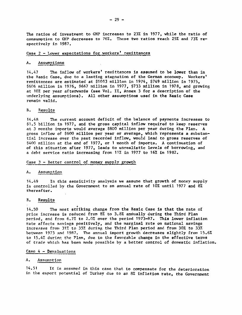
The ratios of investment to GNP increases to 23% in 1977, while the ratio ofconsumption to GNP decreases to 76%. These two ratios reach 25% and 73% re-spectively in 1987.

Case 2 - Lower expectations for workers' remittances

A. Assumptions

14.47 The inflow of workers' remittances is assumed to be lower than inthe Basic Case, due to a lasting stagnation of the German economy. Workers'remittances are estimated at $1013 million in 1974, $749 million in 1975,$606 million in 1976, $667 million in 1977, $733 million in 1978, and growingat 10% per year afterwards (see Vol. II, Annex 3 for a description of theunderlying assumptions). All other assumptions used in the Basic Caseremain valid.

B. Results

14.48 The current account deficit of the balance of payments increases to$1.5 billion in 1977, and the gross capital inflow required to keep reserresat 3 months imports would average $800 million per year during the Plan. Agross inflow of $600 million per year or average, which represents a substan-tial increase over the past recorded inflow, would lead to gross reserves of$400 million at the end of 1977, or 1 month of imports. A continuation ofof this situation after 1977, leads to unrealistic levels of borrowing, anda debt service ratio increasing from 11% in 1977 to 16% in 1982.

Case 3 - Better control of money supply growth

A. Assumption

14.49 In this sensitivity analysis we assume that growth of money supplyis controlled by the Government to an annual rate of 10% until 1977 and 8%thereafter.

B. Results

14.50 The most striking change from the Basic Case is that the rate ofprice increase is reduced from 8% to 3.8% annually during the Third Planperiod, and from 6.7% to 2.0% over the period 1973-87. This lower inflationrate affects savings positively, and the marginal rate on national savingsincreases from 31% to 35% during the Third Plan period and from 30% to 33%between 1973 and 1987. The annual import growth decreases slightly from 15.6%to 15.4% during the Plan, due to the favorable change in the effective termsof trade whichi has been made possible by a better control of domestic inflation.

Case 4 - Devaluations

A. Assumption

14.51 It is assumed in this case that to compensate for the deteriorationin the export potential of Turkey due to an 8% inflation rate, the Government

- 30 -

introduces discreet devaluations of the lira, either through a multiple ex-change rate system or through a change of the official parity. Devaluationsof 20% in the years 1977, 1982 and 1987 have been assumed. Thus, the officialexchange rate becomes TL 14 to $1 until the end of 1976; TL 16.8 to $1 from1977 to the end of 1981; TL 20.2 to S1 from 1982 to the end of 1986; and TL24.2 to $1 in 1987.

B. Results

14.52 The most distinctive change appears in the balance of payments, thedevaluations slow down import growth, and the current account deficit in thebalance in 1977 changes from $774 million in the basic case to $453 millionin this sensitivity run, the average gross capital inflow required to main-tain reserves at a level of 3 months of imports falling to $377 million peryear $475 million in the basic case).

Case 5 - Faster Export Growth

A. Assumption

14.53 It is assumed that export will grow faster than in the Basic Case.The annual export growth rate increases from 8% to 10% over 1974-77 and from9.3% to 12% after 1977.

B. Results

14.54 The clearest response to this change in assumption appears in thebalance of payments. The current balance deficit in-1977 reaches-$593 mil-lion, and change from $33 million to $185 million the average ..gross capitalinflow reaches about $500 million per year. Accordingly.,:the debt serviceratio for 1977 decreases from 7.3% in the basic .case to 6.9% in the presentsensitivity analysis.

Case 6 - Slower Export Growth

A. Assumption

14.55 A slower export growth (6% per year) has been assumed during 1974-87.

B. Results

14.56 The balance of payments situation changes sharply. The gross bor-rowing requirement increases to $550 million per year during -the Plan periodand the debt service ratio rises from 7.3% in the basic case to 7.9% in 1977.After -1977, the borrowing requirements increase rapidly, leading to a debtservice ratio of about 15% 'during the eighties (with a peak of nearly 18% in1982).

- 31 -

Case 7 - Borrowing Terms Hardened

A. Assumption

14.57 It is assumed in this case that the maturity and grace period of allnew loans are shortened by half. Thus, the new terms of borrowing in atypical loan would change from: Maturity = 21 years, Grace Period = 4 yearsto Maturity = 10 years, Grace Period - 2 years.

B. Results

14.58 The gross borrowing requirement increases to $515 million per year($475 million in the basic case), and the debt service ratio increases from73% in 1977 in the basic case to 9.7%, and from 13% to 15% in the eighties.

Table 87: SENSLflTVJ Y Xi,ALYSIS -ESULTS - AVERAGE ANTlrAL GRDWTH RATES (G)

Major 1966-72 1973-1977 1M73-1B 67lndicators Actual Basic Basic

Carse Case 2 Case 3 Case 4 Case 5 Case 6 Case 7 Case Ca-e 3 Case It Case 5 Case 6 Case 7

G?IPlI: 7.1 7.9 7.6 7.9 7.9 7.9 7.9 7.9 7.9 7.9 7.9 7.9 7*9 7.9GDPM4? 6. .1 8.1 8.6 8.1 8.1 8.1 8.1 8.0 8.0 5.0 d.0 8.0 8.0Invest. 7.6 12.3 12.3 12.5 12.3 12.3 12.3 12.3 9.9 9.9 9.9 9.9 9.9 9.9Cons. 6.8 6.S 6.3 6.7 6.8 6.e 6.8 6.8 6.7 7.1 6.7 6.7 6.7 6.7inpt. 13.6 13.1 13.0 13.0 13.1 13.1 13.1 13.1 8.3 8.3 8.3 8.3 8.3 8.313IS 9, 13.3 -12. 14.2 13.5 13.5 1 3.5 13.5 10.4 lo. I 1C.>. lo.L; lo.L. i-O.L;GDS 5.1 13.2 13.8 13.k 13.2 13.2 13.2 13.2 11.2 11. 1 1 1.2 11.2 1 1.2 ll.2-

MSRL 21.8 31./ 30.0 34.0 31.0 31.0 31.0 31.0 30.0 32.0 30.0 30.0 30.0 30.0CGP DE'FL. 10.1 8.0 8.0 3.8 8.0 8.0 8.0 b.0 6.7 2.0 6.7 6.7 6.7 6.7Yoney Supl. 18.6 17.0 17.0 i0.0 17.0 17.0 17.0 17.0 15.0 8.0 15.0 15.0 15.0 15.0

Case 2: Lower workers, remittances, due to lasting recession of the German economy. -Case 3: Mbney supply growth curbed to 1OP per annmu until 1577 and 8% thereafter.

Case 4: Devaluations by 20A have been assumed in 1977, 1982 and 1987.

Gase 5: Export grovs faster - 10% per annum until 1977 and 12% thereafter.

Case 6: Export grows less - 6g per annum until 1987.

Case 7: Brrowing terms hardened - maturity and grace period shortened by a half.

LJ On national savings.

TSable 88. Sensitivity Analysis. Balance of payments projections(million current dollars)

1977Basic case Case 2 Case 3 Case 4 Case 5 Case 6 Case 7

Imports (goods and nfs) 4497 4469 4474 3762 4506 4488 4497Exports (goods and nfs) 2484 2484 2484 2070 2673 2305 2484

Interest on debt 124 175 124 124 124 134 123Workers' remittances 1400 667 1400 1400 1400 1400 1400

Current account balance -774 -1530 -751 -453 -594 -954 -772

Gross public capital inflow -/ 899 1700 845 410 498 1152 1039official 1/ 410 410 410 410 410 410 410suppliers- 482 1300 435 - 88 715 629

Amortization 165 165 165 165 165 165 260

Net public capital inflow-/ 727 1535 680 245 333 437 773

Overall balance of payments 91 152 66 -70 -123 144 144(minus means decrease inreserves)

- Due to the structure of the model, suppliers' credits have an irrular pattern, while reservesincrease regularly. Average flows of suppliers' credits over a time period are therefore moremeaningful than yearly estimates.

Table 89: SENSITIVITY ANALYSIS - SELECTED RATIOS (%)

1977 19871972 Basic Basic

Ratios Actual Case Case 2 Case 3 Case 4 Case 5 Case 6 Case 7 Case Case 3 Case 4 Case 5 Case 6 Case 7

Inv/GNP 18.4 23.0 23.6 22.8 22.8 23.0 23.0 23.0 25.2 24.8 24.9 23-9 25.2 25.1

Con/GNP 81.0 76.1 76.4 (5.2 76.0 76.1 76.1 76.1 73.2 71.6 73.1 73.2 73.2 73.2

Imp/GNP 9.0 11.2 11.44 11.1 11.2 11.3 11.2 11.3 9.3 9.2 9.3 9.5 9.4 9.5

RG/GNP 2.9 4.2 4.3 4.2 4.3 3.8 4.8 4.3 1.4 1.3 1.4 -i.1-! 4.0 1.4

GNS/GNP 18.9 23.9 23.6 24.8 24.0 23.9 23.9 23.9 26.8 28.4 26.9 26.8 26.8 26.8

GDS/GDP 16.7 21.1 22.6 21.3 20.6 21.1 21.1 21.1 25.7 26.4 25.0 25.7 25.8 25.7

DS/X+W 11.6 7.3 10.6 7.3 8.1 6.9 7.9 9.7 10.9 9.6 8.5 4.4 34.8 14.9

DS/X 21.4 31.3 13.4 1.3 13.6 10.5 12.7 15.1 14.0 12.3 12.7 5.3 49.1 19.1

TURKEY MACRO MODEL RUN NO. 1 _ BASiC CAS4-6 DATE u 01/10/74 CLOCK TIME * 12,33,52,-

1973 1974 1975 1976 1977 1982 1987

NATIONAL ACCOUNT SUMMARY(1968 TL BILLION)

2 VAl 36,980 38,460 39,998 41,596 43,262 52,635 64,0387 VA2 31,399 34,852 36,686 42,942 47,665 80,319 135,342

12 VA3 15,844 17,031 18,298 19,661 21,125 30,251 43,31934 VA 4 50,234 54,253 58,593 63,80o 68,343 100,418 147.547

16 GDPFC 134,457 144,596 155,576 167,481 180,395 263,622 390.246

22 IT 18,345 19.713 21,196 22,803 24.546 35,782 52,876

18 GDPMP 152,801 164.309 176,771 190,284 204,941 299,404 443,122

19 GNPMP 159,216 171,082 183,864 197,661 212,529 306,243 449,320

33 TOTL.I 32,933 38,326 41,561 45,084 48,925 74,061 113,144

17 Fl 29,985 32,480 35,221 38,207 41,462 62,763 95,88563 IP 2,948 5,846 6,340 6,877 7,463 11,297 17,25942 TC 124,832 132,655 141,437 151,149 161,692 227,967 329,004

41 PC 101,476 107,754 115,016 123,948 133,581 164,687 263,27040 GC 23,356 24,981 26,867 29,011 31,415 47,705 73,07548 TOTL M 15,838 18,498 19,357 2t,458 23,775 30,128 42.36855 XPT 10,675 11,745 12,685 13,699 14,795 23,079 36,00253 NFI 6,415 6,773 7,093 7,378 7,588 6,839 6,198

BALANCE OF PAYMENTS SUMMARY (CURRENT US MILLION DOLLARS)

71 M+NFS 2424,345 3131,389 3415,178 3920,669 4496,907 6768,045 11304,11072 X+*'FS 1621,929 1804,233 2007,029 2232,619 2483,566 4491,202 8121,148

146 I-TOTL 99,280 94,937 96.426 103,373 124,151 241,766 409,45578 PR-TR 41,000 42,230 43,497 44,802 46,146 53,496 62.01680 WRS 900,000 1005,000 1123,000 1254,000 1400O,00 1786,794 2280,45282 NATO 10,000 10,000 10,000 10,000 10,000 10,000 10,000

113 D-OTH 12,000 20,000 20,500 20,500 20,000 20,000 20,000

95 CAB -32,697 -449,323 -415,071 *572,225 -773,639 -775,310 -1363,381

159 D-S/C ,000 0,000 0,000 0,000 481,903 622,120 1376,55981 DIR 1 44,000 45,100 48,000 51,000 55.000 70,195 89,58983 IMWW 41,000 43.870 46,941 50,227 53.743 75,377 105,720

114 OFFOIS 379,650 338,050 366,450 390,250 410,200 431,685 458,01284 TLGRN 20,000 22,000 24,000 26,000 28,000 32,460 37,630

160 GRANAM 212,500 220,000 190,050 133,000 164,658 347,849 732,770

104 NKINFL 272,150 229,020 295,341 384,477 864,187 972,363 1712,967

101 OVLBAL 239,453 -220,303 -119,730 -187,749 90,549 197,053 349,586

158 RS-CH -239,453 220,303 119,730 187,749 -90,555 -197,124 -349,687

MACRO ECONOMIC INDICATORS

115 DS/XW 7,387 6,993 6.741 6,579 7,256 9,280 10,913116 DS/X 11,486 10,889 10,513 10,274 11,347 12,972 13,978117 M/GNP 9,947 10,812 10,528 10,856 11,187 9,838 9,429118 RG/GNP 3,117 3,947 3,629 3,925 4,225 2,302 1,417119 TC/GNP 78,404 77,539 76,925 76,469 76,080 74,440 73,223120 I/GNP 20,684 22,402 22,604 22,809 23,020 24,184 25,181121 NS/GNP 21,596 22,461 23,075 23,531 23,920 25,560 26,777122 S/GOP 18,305 19,265 19,988 20,567 21,103 23,860 25,753123 GR-PY 9,762 8,195 8,173 8,148 8,123 6,070 5,958

AVERAGE LOAN TERMS AND GRANT ELEMENT.. .. .... .,............... .. ... . . .

1 MAT, 22,866 20,663 20,774 20,783 13,971 13,493 11,4752 INT, .,052 ,052 ,053 .054 ,059 ,059 .0613 GRACE 3,927 3,928 3,929 3,928 2,892 2,804 2,501

4 GR,EL, 3i,483 30,36 30,165 29.670 20;733 i9,ss3 Y-s79075 (1) 31,483 30,386 30,165 29,670 20,733 19,953 17,907

(l) GRANT ELEMENT. GRANTS EXCLUDED

TURKEY MACRO MODEL RUN NO.,S DATE * 01/10/74 CLOCX TIME a 23.13,40.

1973 1974 1975 1976 1977 1978 1979 1910 1961 1962

NATIONAL ACCOUNT SUMMARY(1968 TI. BILLION)

2 VAl 36,980 38,460 39,998 41,596 43,262 44,992 46,792 46,664 50.610 52,6357 VA2 31,399 34,852 38,656 42,942 47,665 52,908 58,728 65,188 72,359 80.319

12 VA3 15.844 17,031 18,298 19,661 21,125 22,698 24,388 26.204 26.155 30.25134 VA 4 50.234 54,253 58,593 63,280 68.343 73.810 79,715 86,092 92,950 100,41616 GOPFC 134,457 144,596 155,576 167,481 180,395 194,409 209,623 226,148 244,104 263,62222 IT 18,345 19,713 21,196 22,803 24,546 26,438 28,492 30,723 33,147 35,78218 GL)PMP 152,801 164,3 09 176 ,7 71 1.90,284 204,941 220,847 238,115 256,871 277,250 299,40419 GNPMP 159.216 171,145 181,166 193,338 207.694 223,266 240,498 259,270 279,685 301,682

33 TOTL I 32.933 38,326 41,561 45,084 48.925 53,114 57,684 62,672 68,116 74,06117 FI 29,985 32,480 35,221 38,207 41.462 45,812 48,885 53,112 57,725 62,76363 IP 2,948 5,846 6,.340 6,87 7 7,:463 8.1102 8,799 9,560 10,391 11,29742 TC 124.832 132,693 139,776 148,487 158.716 169,709 181,876 195,145 209,563 225,28241 PC 101,476 107,764 114,575 123,621 133,436 139,731 149,206 159.866 171,668 184,61640 GC 23,356 24,981 26,867 29,011 31,415 34,086 37,034 40,274 43,624 47,70548 TOTL M 15,838 18,508 18,916 21,131 23,630 22,255 23,484 25,263 .27,473 30,05755 XPT 10,875 11,745 12,685 13:699 14,795 16,171 17,675 19,319 21,116 23,07953 NF 1 6,415 6,836 4,395 3,054 2,753 2,419 2,383 2,399 2,435 2,478

BALANCE OF PAYMENTS SUMMARY (CURRENT US MILLION DOLLARS)

71 M.NFS 2424,345 ~~~~~ ~~313308 3337,308 38;61,010 4469,441 4356,781 4758,286 5297,704 5962,907 6752,05172 X+NF S 1621,.929' 1804,233 2007,029 2232,6t9 2483,566 2795,973 314 7 .879 3543,625 3989,376 4491,202

146 I-TOTL 99,280 94,937 96,426 103,373 174,760 269,957 322,949 372,405 423,964 460,25878 PR-TR 41,.0 00 4 2,23 0 43,497 4 4, 802 46,146 47,530 48,9 56 50,425 51,938 53,49680 WHI 900,000 1013,000 749, 0 00 606 , 000 667,0 0 0 733,.7 00 8 07 .070 887,777 976,555 1074,210

82NTO 10,000 10.000 10,000 10,000 10,000 10.000 10,000 10,000 10,000 10,0001 W!OTH ~~12,.0 00 2 0, 00 0 20,5 00 2 0,.50 0 20, 0 00 2t.0,000 20,0 00 2 0, 00 0 20 ,0 00 20,000CAB -32,697 -~~~~~~~443.U18 -711,202 *1160.566 -1529,782 -1134,594 -1165.442 -1279,131 -1462,86-71,9

159 C-S/C ,fl00 0.000 o,ooo ~~~~~~~~~~~~~~~-9 741,108 912,537 1055,841 1269,390 15,581 DIR I ~~~~~~44.000 45,100 48,000 '51,E0700 ' .55,000 57,750 60,637 63,669 66,653 70,195

83 IHlWw 4 1,0 0 U 43.870 46,941 50,227 53,743 57,505 61,530 65,837 70,446 75,377114 OFFCIS 3 79,6 50 338, 05 0 366,450 39 0 ,25 0 41 0,.200 417,650 4 19 ,7 00 426,050 428,744 431,68584 TLGRN 20,000 22,000O 24,.0 00 2 6,00 0 '28,.000 28,840 29,705 30,596 31,514 32,4601,60 GRANAM 2 12,5 00 22 0,00 0 190,050 133,000 164,658 312,104 519,661 635,253 775,418 947,89110 4 NKINFL 2724150 22 9,02 0 295,341 1194,229 1681.886 1 106, 42 7 1265,785 1413,950 1629,105 1907,5999

101 OVLOAL 239 ,453 -213.998 -415 .861 33,663 152,105 -28,167 1 00,3 43 134, 819 166,229 197,206158 RS-CH -239,453 213,998 415.861 -33,658 -1J2.i08 28,165 -100,376 -134,854 -166,301 -197,286

MACRO ECONOMIC INDICATORS

115 CS/OW 7 .387 6, 97 3 7.o56 8, 08 0 10.551 16,292 21,129 22,581 24,011 25,5351.16 OSlX 11.486 1q.889 10,513 10,274 13,385 20,567 26,547 28,238 29,889 31,643117 M/GNP 9,947 10,814 10,441 10,930 11,377 9,968 9,765 9,744 9,823 9,956118 RG/GNP 3,117 3.951 3,440 3,844 4.254 2,725 2,415 2,292 2,273 2,311119 TC/3NP 7o,404 77.033 77.154 76,802 76,418 76,012 75,625 75,267 74,935 74,626120 I/GNP 20,6b4 22,394 22,941 23,319 23,556 23,790 23,985 24,172 24,354 24,533121 NS/GNP 21.596 22,467 22,846 23,198 23,582 23,988 24,375 24,733 25,865 25,374122 S/GOP 16,305 19,242 20,9 28 21,965 22,555 23,155 23,618 24,030 24.406 24,757123 GR-PY 9,762 8.195 8.173 8,148 8,123 6,.165 6.141 6,117 6,094 6,070

AVERAGE LOAN TERMS AND GRANJT ELEMENT

I MAT, 22,866 2n,663 20,774 12,332 11.123 12,707 12.101 11,792 11,366 10.9252 INT, .052 .052 .053 .059 .060 .060 .D60 .060 .061 .0613 GRACE 3,927 3,928 3,929 2,653 2,.4 67 2,698 2 .608 2,559 2,494 2,428

RUN 40 3- *ETTER CONTROL Of MONEY SUPPLY DATE * O1V10i74 CLOCK TINE * 12.34.09.

1973 1974 1?7? 1976 1977 1962 1Q87

NATIONAL 4CCOUNT S'JNMARYn9Ga TL BILLION).._......._.____.___._____ _._____.. ___ _

2 VAI 36.980 308460 39.998 41,590 43,262 52,635 64.038

7 V62 31,399 34,852 30.686 42.942 47,665 80,319 135.342

12 VA3 15.844 17.031 18.295 19.661 21.125 30,25± 43.319

34 VA 4 50,234 54.253 58,593 63,280 68.343 100,418 147.S47

16 OUPFC ±34,457 144.596 155,576 :67, 81 180.3v5 263,622 390.246

22 IT 18.349 19.713 21,196 22.8u3 24,5- 35,782 52.876

18 GDPAP 192,401 164,309 176,771 190,284 204.941 299,404 443.122

19 (ANPMp 159,216 171.689 184,838 1;O,042 214.343 309,734 454.545

33 TOTL I 33,1.83 30,326 41.561 45.084 48.925 74,061 113.144

17 Fl 29.985 32.480 35.221 38.207 41.462 62,763 95,885

63 IP 3.,98 5.846 6.340 6.877 7.463 11,297 17,259

42 U' 124.581 132.498 141.194 150.808 161,433 226,476 325.664

41 PC 101.22 107.783 114.968 123.665 133.462 l84,360 262.716

40 (GC 23.356 24.981 26,667 29.01C 31J415 47.705 73.075

48 TnTfL N 19,.30 18.527 19,309 21.376 23.657 29,801 41.815

55 EPT lO.875 11.745 12,685 13.699 14,795 23.079 36.002

S3 WFI 6.415 7.380 6.067 8.758 9-402 10,330 11,423

BALANCE OF PAYMENtTS BUtMMA4I (CURRENT US MILLION DiOLLARS)._._._._.............__ ._.__......................._.__......... ___.._____

71 .14.FS 2424.445 3136,308 3406,744 3905,682 4474,489 6694,674 11156.545

72 KeNFs 1621.929 1404.233 2007.029 2232,619 2483.586 4491,202 8121.748

146 I IsT0L 99.280 94.937 96.426 103.373 124.151 226.607 370.608

78 PP-TR 41.000 42.230 43,497 44.802 46,146 53.496 67.016

80 *di1 900,4100 100l.000 1123.000 1294.000 1400,0CO 1786,794 2280.452.

82 NATLO 10.100 1n.000 o 1.0CO 10.000 10.000 10.000 10.000

t13 D-JOt 12,000 20.000 20.500 20.500 20.000 20.000 20.UOo

95 C04 -32.697 -454.242 -4C6,63B -557.273 -751.220 -6866780 -1176.969

159 U-WsC .O00 3.000 0DOGU LO,OC 435.377 530,904 1168.127

61 Llik I 44.0OC 43,100 48.f01 51.000 55.0t,io 70.195 89,589d3 1AIw 41.dCJ 43.870 46.041 5n.227 53.743 75.377 105,720

114 uFrOIS 37s,V.su 33,050 366,450 390.250 410.200 431,685 458.012

84 TUSRN 20.0u0 22.000 24.000 26,000 28,000 32,460 37,630

160 CRANAN 212.500 220.000 190.050 133,000 164,658 321.672 633,273

$q4 NAItFL 272,150 229.020 295,341 384,477 017,661 681,147 1522.535

181 OVLSAL 239.453 -225.222 -111.297 -172.761 66.441 194,367 345.567

1s6 0S-CW4 a239.453 225,222 111.297 172.761 -66,449 -194.425 *345.654

MACRO EC3NONlC INDICATORS... ..... _.......... _...

11s US/vI 7 .I7 6,993 6,741 6.579 7.256 8.622 9.583

1l6 /1% 11,486 1j.689 10.513 10,274 11.347 12,052 12.274

117 '/CINP 9,047 10.791 10.447 10,739 11.037 9,622 9.199

118 RG/JsSp 3.tl7 3.950 3,584 3,657 4.134 2,170 1.279

119 TC/GNP 7e.47 77.173 76,388 75.767 75.Z22 13J,19 71.646

120 IfGNP 20.,42 22.323 27,405 22.650 22.026 23.911 24.892

121 NSIG;NP 21.75J 24,827 23.612 24.233 24,778 26,881 20.354

122 S/QJP 18,466 19.361 20,126 20.746 21,327 24,35B 26,507

123 9O-PY 5.155 3,654 3,633 3,609 3.585 2.158 2.050

AVERAGE LOAN TERaS AND GRANT ELEMENT....... ............. ...... ,. ..

1 MAT, 2,e866 20.663 20,774 20.783 14.297 14.007 11.872

2 ' .052 .052 .053 .054 .058 .059 .060

3 1.-'ACE 3.g27 3.928 3.929 3.92b 2.941 2.879 2,558

4 *4.:L, 31.483 30.386 30.165 29.670 21.094 20.487 18.287

5 t1) 31,4a6 30.536 30.165 29.670 21.n94 2n.487 18,287

(t) L.&PY ELEMENT, GRANTS &.XCLUDED

RUt NO 40 ifEVALUATIONS ASSutlt) DATE * 01/11/74 CLOCtt TIME * 12.34,19.

1973 l974 1975 1976 1977 1982 1987i

ttATIONAL ACCOUNT SUMpjARY( 19'8 TL tILL1IO;.......... ........................................... ,

2 VAI 36,'tbJ 311.460 39.996 41.598 43.?62 52.635 64.0387 V2 31.399 34.652 38.686 42.942 47.665 80,319 135. 42

12 VA3 15.844 17.031 18.298 19.661 21.125 30.251 43.31934 vA 4 50.'!34 54.253 58.393 63.280 66.343 100.418 147.54716 G'.PFC 134.457 144.596 155,576 167,481 180.395 263,622 390.24622 IT 18.S45 19.713 21.196 22,803 24.846 35,782 52.676la st,ipP 152.401 164.309 176.771 190.284 204.941 299.404 443.12219 I1NP4P 159.?16 171.082 183.364 197.661 214.J46 309.578 454.797

33 TOTL I 32.433 31J.326 41.61 4i.084 48.v25 74,061 113.14417 fl 29.985 32.480 35.221 38.207 41.462 62,763 95.b8563 IF 2.940 5.846 6.340 6.877 7.463 11,297 17.25942 T; 124.;j32 132.655 141.437 151.149 162.627 230,020 332.37741 PC 101.476 iO7.754 115.J16 123.948 133.673 184,619 263.0144300 23.356 24.981 26,N67 29.011 31.415 47.705 73.07546 TOTL M 15.83 1d.498 19.357 21.458 23.867 30.061 42.11355 XPT 10,h75 11.745 12^685 13.699 14.795 23,079 36.no253 ttI 6.115 h.773 7.093 7.376 9.105 10.174 11.e.76

BALANCE OF PAYMENTS SUNMAj(y (CUkRENT US MILLION DOLLARS)......... ..................... _....., _ _.....

71 %+NFS 2424.345 3131.389 3415.17b 3920.669 3761.923 4680,204 6500.16272 X*NFS 1621.929 1804.233 2007.u29 2232.619 2069.638 3112.714 4698.532

146 1-TOTL 99.260 91.937 96.426 103,373 124.151 195,604 246.6907d P.#-TR 41.GOO 4k.230 43.497 44.802 46.146 53.496 62.016aU lJp 900.000 1005.000 1123.loo 1254.000 1400.u00 1786,794 2280,45282 pATO 10.UUC nl.000 10.000 0,000 10.000 10,000 10.0 00113 U-OTW 12.-°00 20 0o0 20.500 20.500 20.U0o 20.000 20.noo9s cAE -32.*97 -449.323 -415.J 7 1 -572.225 -452.582 -19.795 179.916

159 D-s/C .010 U.000 0.000 n.000 0.000 0.000 0.00ott 8IR 1 44,000 45.100 48.000 51,000 55.000 70,195 89.589843 I-.. 41. r, 0 43. 670 46. '41 50.27 53.143 75.377 105.720

114 (FFUIS 379.65u 338.050 366.450 390.250 410.200 431,685 458.11284 TLG4N 20.000 22.000 24.000 26,000 28.000 32.460 37.630

160 .RA#NAM 212,jOU 2211.000 190.050 133.000 164.658 259.475 356.543104 :I NFL 272..LSC 22u.020 295,341 384.477 382.285 350,243 334.406

101 OVLOAL 239.453 -22t.303 -119.730 -187.749 -70.297 330,447 514.324158 hS-C14 -239.453 2211.303 119.730 187.749 70.297 -330,447 -514.324

MACRO ECONOMIC INDICATORS

115 5/XIJ 72,3S7 A.993 6.741 6,579 8.122 9.145 8.!40116 DSIA 11.4t6 10.889 10,513 10,274 13.A16 14.395 12.694117 M/GNP 9.947 16.812 10.528 10.856 11.150 9.710 9.260118 RiGq#N0 3.117 3.947 3.629 3.925 4,238 2,255 1.344119 TC/GNP 78.404 77.539 76.925 76.469 75.977 74.301 73.1'82120 1 /GIP 20.6b4 2c.402 22.604 22.809 22.857 23.923 24.C78121 NS/GNP 21.596 22.461 23.1175 23.531 24.,123 25,699 26.918122 5/G9P 1(.JtS 14.265 19.988 2r.567 20.t47 23.174 24.992123 GR-PY 9.762 0.195 8.173 8.148 8.123 6.070 S.V58

AVERAGE LOAN TERMS AND GRAt.I ELEMENT

M MAT. 22.h66 20.663 20.174 20.783 20.904 21,200 21.4492 ; T . .1,52 .052 ,u53 .054 .G54 .055 0553 GRACE 3.927 6.928 3.929 3.928 3.928 3,932 3.9384 Gk.EL. 31.483 3C.3o6 30.165 29.670 29.389 29.097 29.2465 (1) 31.483 30 .386 30.165 29.670 29.389 29,097 29.246

(1) GNANT ELEMENT, GRANTS EXCLUDED

RUN NO *9 'MORE EXPORT GROWTR. DATn. : 0110/74 CLOCK TIlMt. 12.34.27.

!973 i974 1975 1976 1977 1982 jqb7

NATIONAL ACCOUNT SUMMAkY(1968 TL BILt ION)----- _-_------__--____..--_---_-------__.

2 VAt 36.S80 30.460 39.998 41.598 43.,'62 52.635 64.0387 VA2 31,399 54.852 38.686 4?,942 47.A65 80.319 135.342

12 vA3 15.t44 17.031 18.298 19,661 21.125 30,251 43.51934 VA 4 50. 34 54.253 58.,593 63.280 68.343 100.418 147.,471 (,ILPF C 134.457 14'..596 155.t76 167.481 180.395 263,622 390 .24622 IT Ihb,34S 14.713 21.196 2;.,s3 24.546 35,782 52.t761H bLLPMP 152. tU1 164.309 176.771 19C.2b4 204.941 299.404 443.iZ219 GhkP'tp 159.i16 171.082 183.1t64 197,661 212.529 306.441 449.d76

33 TrTL I 32.9)3 31 .219

41.561 45,084 4e.s25 73,528 lU7.J0717 VI j9,985 32.480 35.221 38.207 41.462 62.763 95.al8563 rf' 2.948 5.739 6,340 6,877 7.463 10.767 11.1254; TC 124,832 13,.655 141,437 151.149 161.o92 228.089 329.34741 PC 101.476 107.674 114.S77 12.i,213 132.5O2 180,384 256.27240 f0NL 2.es o 24.98 1 26.1667 20,011 31.415 47,705 7J., u7548 TUTL M 15.e3d lh1.527 19.392 21.499 23.1f23 30,275 42.6P`655 AP T 1U. t,7:7 1v. 92 13.159 14 , 4 75 15.222 28 , 060 4 9 .45 253 FI 8. '15 h,773 7.tl93 7.378 7.588 7,038 6,755

BALANC8 OF PAYMENTS SUMltMAHY (CUkkEN( US MILLION LOLLARS)-____--__-__---__-_--_-_-_----_---,,-------__--_-------_-

71 : NFS 2424.345 J136. 396 3421.336 3928.152 4505.949 6800.965 11368.,JO772 V+qF s 1621.029 lb3/.645 2082.052 2350.965 2672.707 5460.440 11155.18o

146 I-TOTL 99., 8u 9,.937 96.426 103.373 124.J51 198,548 246, 8 9078 P8-TR 41.110O 42.230 43.497 44,802 46.146 53.496 62 .16O0 El i 90O 0.uot0 1005.UEO 1123.600I 1254.000 1400. '00 1786.794 2280.45282 AT'J 10. .U0 1n.000 10.000 1U.000 1000 0 10.000 10.000

113 U-"I r 12.,rou 2tU. U00 20 .500 21!.500 20 .000 2no.000 20. JOO95 CAb -32.697 -420 .918 -346.206 -453,.362 -593.539 204.224 1748.619

159 -S/c (,G00 U .UO 0.000 (o. uOG 67.c32 o,000 0.JOO81 aln I 44.U,UU 45.101) 48.OO 51.000r 55.000 70.195 89.58983 I,;^ 41,1100 4 . 670 46.941 51.227 53.743 75,377 105.720

114 OFFlOIS 379,65u 33t..tTh0 366.450 39t,250 410.200 431.685 458.L,1284 TLtiRN 20.1:00 22,0no 24.(600 26.000 28.,100 32.460 37.630

160 GPANAM 212.50u 22' .000 190.050 133.000 164.658 272.037 356,543104 NK1.'FL 272.15u 22Y.070 295.341 384,477 470.217 350.243 334.406

181 OVLOAL 239.'.53 -191.898 -50.h.65 -61.,s6 -123.323 554.467 2003.127158 'S-CH -239.453 141.89e 50.865 6th.b65 123.317 -554.467 -20ts.U27

MACRO ECONtOMIC INDICATONS

115 'S/)w 7. ts7 8.911 6. 183 6.349 6.919 6.397 4.43911t6lt 4/A 11 .46 1L.61 10t.134 9.723 1 0.544 6,490 5.346117 7YI,NP 9.947 1rO. k2 9 10.547 1G.877 11.209 9.879 9.48811t ?,/GNP 3.;17 '.tL 3.7 3 ..-90 . .554 3.718 .723 -1. 504119 TL / NP 7b,u. 4 77.5ff9 76,925 76.4o9s 76.C80 74.432 73.206120 I/G'.P 2u0.64 22.339 22.h04 22.809 23.j2O 23.994 23.786121 .45/GNP 21.S96 22.4e4l 23.n75 23.531 23.920 25 568 26.792122 S/G'lP 1o ..05 19,265 19.988 2 .567 21.103 23. 819 25.676123 GP-PY 9.762 1. 195 8.173 8,146 8 ,123 6.070 5.958

AVERAGF LOAN TERMS AND GHAI'l eLEMr NT

1 -'AT. 22.mhO 20 . 663 20. 174 21 .783 18 .647 21,200 21.4 497 1jT, (.5 2 .052 .rl53 . 054 .1156 .055 .n553 GPACE 3.92 7 3.928 3.929 3.928 3.591 3,932 3. a?384 t,R, EL* 31. 4 0. 30. 3d6 30.165 29.670 26.326 29,09i 29 , 2 465 (1) 31.4bJ 3-i.386 30.165 29.670 26.326 29.097 29,246

tt) GRANT ELEMENT, GRANTS EXCLUUED

RUN 6 6 PEq CE-NT EXPORT GROWTH DATE a 0I/10/74 CLOCK TIME 1 12.35.28.

1973 1974 I975 1976 1977 1982 1987

NATIONAL ACCOUNT SUMMARY(11;6 TL BILLIUM)

2 VAI 36.980 36.460 39.99b 41,59e 43.262 52.635 64.0387 VA2 3.3j99 34.852 38.686 42,942 47.665 80,319 135.342

12 VA3 15.444 17.031 18.298 19.661 21.125 30,251 43.31934 VA 4 50,234 54.253 58,593 63.200 68.343 100.418 147.54716 UoFrc 134.457 144.596 155.576 167.481 180.395 263,622 390.24622 IT 18.345 19.713 21.196 22,803 24.546 35,782 52.87618 GU9DP 152.001 164.309 176.771 190.284 204.941 299.404 443.12219 GNW'IP 159.216 171.082 183.864 197.661 212.469 305.648 447.684

33 TOTL I 32,9 3 36.326 41.561 45,084 48.925 74.061 113.14417 ri 29.985 32.480 35.221 38,207 41.462 62,763 95.88563 IP 2.94e 5.846 6.340 6,877 7.463 11.-297 17.25942 TC 124.83J 132,655 141.437 151,149 161.656 227,600 327.99741 PC 101,470 107,942 115.448 124,656 134.602 189,253 274.41740 rC 23.J50 24.Q-1 26,867 29,011 31,A415 47,705 73.07548 TUTL 04 15. 0 $ lb.468 19.*24 21.420 23.730 29.988 42.10155 XtT 10j,A7t 11.527 12.219 12.952 13.729 1j8373 24.58753 %Fj 6.415 o.773 7.093 7,37b 7.528 6.244 4,562

OALANCR OF PAYMENTS SUMMARY (CURRENT US MILLION DOLLARS)

71 '.FS 2424.345 3 12o.3V1 3409,228 3913.671 4488.429 *6736.557 11232.804

72 X*NFS 1621.929 1770.i22 1933,383 2110,868 2304,645 3575,358 -5546.704146 I-TOTL 99.2bu 94.937 96,426 103,373 133.876 371,630 886,838

78 Pf,-TR 41.0GU 42.230 43,497 44,802 46.146 53.496 62.'01660 wwI 900,00 1005.000 1123,000 1254,000 1400.000 1786,794 2280,45282 A TO 10.IWO if 10.000 1O,OOO lfaooc 10.'070 10,000 10,000

113 10-UTr 12,00u 20.000 20.500 2C,500 20.000 20,000 20.00095 CAn -32,697 -477,727 -482,768 -606,979 .953.bO6 -1789,.530 -4344.502

159 Ui-S/C ,ooIJ U.000 0.D00 155,595 715.205 1635,090 4357.1O9.81 010 I 44,n0u 45,100 48,000 51,000 55.000 70,195 489.589:83 IMtt 41, 110 43.870 46.941 50.227 53.743 75,377 105.720114 OFFuIS 379.450 33s.050 366.450 390,250 410 .200 431,685 458.012if4 TLGiN 20,eCo 22.0CO 24,COO 26,000 28,000 32,460 37,610

160 6iANA'A 212.5ti" 220,000 190.059 133,000 164.658 :586.'927 -1'844,224104 NKIAFL 272.15,; 229.020 295.341 540.072 1097.490 1985. 333 4691.5.17

101 9vLA4L 239,4593 -24,.707 -1t7.427 -146,,9C7 143 .684 -195.s02 347.U16.s6 4S-O-t -239.43J 240.7n 7 167.427 146,902 -143. 689 -1ff586.4 -347,096

-MACRO E':ONOMIC INDICATORS,,,,. , __ .. _.. _....,._ ... _.

-11% US/Xw 7 .38b7 7.077 6.903 6,817 *7.869 17,746 34.803116 S /x 11.406 11.094 10.913 1n,866 12,650 26,61'4 49.1-1-i117 mlG:N P 9,947 1J,79w5 10 .10 10,837 11,169 9.811 9.404-118 8G/GNP 3,117 4.057 3.864 4,284 4,707 3,800 3.912.119 TC/GNP 78,404 77.539 76,925 76.469 76,.084 74,465 73.,265120 I/GNP 20.0d4 22.402 22.604 22,809 23.n27 24,231 2b.273121 J,S/GNP 21.596 22.461 23.075 23.531 23,916 25.535 26.73'1,22 S/6UiP 18,305 19.265 19,988 20,567 21.121 23,982 25,980123 GR-PY 9,762 8.195 3.173 8.148 8.,123 6.070 5.958

AVERAGE LOAN TERMS AND CiRANT ELEMENT__.__...._ ... , .__.__.____. .__..

1 'IAT, 22,806 20.663 20.774 17.297 12.738 40,816 9.335.2 12!T. 5rJ5 .052 .053 .056 .059 .061 .0623 GRACE 3.9Z7 3.928 3.929 3,402 2.708 2.412 2.1924 G,EL. 31,4dJ 30.386 30.165 24,923 19.'406 4i7,31)5 15,9405 (1) 31,4e3 30,386 30.165 24.923 19.406 17,315 15,940

(1) GhANIT ELEMENT, GRANTS ExCLUDEU

RUN NO 1 PORROWING TERM CHANUE DATE s 01/10/74 CLUCK TIME * 12.35.49.

197J 1974 1975 1976 1977 1982 1987

NATIONAL ACCOUNT SUMMARY(1968 TL 8ILLI uN -

2 VAI 36.980 36.46U 39.998 41.598 43.262 52,635 64.0387 VA2 31.399 34.852 38.686 42,942 47.665 80,319 135.342

12 VA3 15.844 17.031 18.298 19,661 21.125 30,251 43.3l934 VA 4 50.2,4 54,253 58,593 63.280 68.343 100,418 147.54716 fLPFC 134.457 14i..596 155.576 167.481 1bO.t95 263,622 390.e4622 IT 18.345 19.713 21.196 22.803 24.546 35,782 52.87618 GUP1P 152.801 164.309 176.771 190.284 204.941 299,404 443.122

19 Gt.Pl"P 159,.21 171.082 183.863 197.671 212.536 306,136 44v.128

33 TOTL 32.933 3e.326 41.561 45,084 48.925 74,061 113.14417 Fl 29.9025 32.480 35.221 38,207 41,462 62,763 95.88563 IP 2.948 5.846 6.340 6.877 7.463 11,297 17.25942 TC 124.832 132.655 141,436 151,155 161.697 227.901 328.88641 FC 101.47O 107.754 115.D16 123,948 133.581 184,684 263.26540 GC 23.3be 24.981 26.867 29.011 31.415 47.705 73.07548 TOTL . 15,83t, 1d.498 19,357 21,458 23,775 30.125 42.36455 xPT 10.87t i1,745 12.685 13.699 14.795 23,079 36.002

53 NFl 6.415 6,773 7,091 7,387 7.596 6.733 6.006

SALANCk OF PAYMENTS SUMMIARY (CURRENT US MILLION DOLLARS)........................ ............................................. ____ ....__,_

71 $NF S 2424,345 3131.389 3415.170 3920,711 4496.943 6767,458 11302,85872 W+%FS 1621.'29 1804,233 2007,029 2232,619 2483.566 4491.202 8121.748

146 I.TUTL 99.280 94.937 96.679 101,963 122.908 265,087 465.55878 P.-1q 41.60O 42,230 43,497 44.802 46.146 53,496 62.0160o 1.Ht 900.0ou 1005.000 1123.000 1254,000 1400,U00 1786,794 2280.452

82 .AT(,T 1. PU II).0110 10,.Ot, 10.000 o.roo I 10,000 10.000113 Ll-OTH 12',(O 20.000 20.!0C 20,500 20.c00 20.000 20.000

95 CAb -32.697 -449.323 -415.316 -57 ,857 -772.431 -798,045 -1418.232

159 )-S/C ,t00 c.nno 0.(OC 6.248 629.t65 873.305 1639,32381 *I"W I 44,01ou 4,.100 48.,(00 51,000 55.u100 73,195 89,589S3 Iltlw 41,CU0 4;'.870 46.941 5s.227 53.743 75.377 105.720114 (:FFitIS 379.651 33t.050 366.450 39s,25s 410.200 431.685 458.012

F4 TL U N 20.zou 2,.000 24.100 2ti.000 28.1,00 32.460 . 37.630

16C (. IAN AM 212.t'0U 22.. 4U1O 227. b24 20t,.897 259.725 608, 632 1090.447104 K I '1FL 272.:50 22 .oJ0 258.a67 371.828 916.483, 995.066 1767.107

101 OVLJA. 239.,153 22!i.3U3 -156.949 -199.029 144.352 197,020 349,574158 R S-CH -239. '.53 22-,.303 156.949 19. .024 -144. 05A -197*092 -349,675

MACRO tCONONIC INDCliATORS..........................

115 9)S/XW 7,;87 1.171 7.930 a,658 9.o72 13.806 14.091116 USIA 11.486 11.lt6 12,368 13.520 15.125 19,298 19.072117 II/GNP 9.47 i1j.fi2 10,528 10.855 11.18O 9.841 9.43211.4 kl';/,NP J.W7 1.947 3.629 .',925 4.?25 2,302 1.416119 I%/iNP 78,404 77,539 76,925 76.468 76,1380 74,444 73.228120 I/GNP 20.8d4l 2?.402 22.,04 2?,808 23.120 24.192 25.!92121 NS/GNP 21.;90 2?.461 23.175 21.532 23.920 25,556 26.772

122 S/jJP 1d.305 1'.265 19t.989 20,564 21.101 23.882 25.780123 GR-PY 9,762 i.195 8.173 8,148 8.123 6,070 5.958

AVE8AGE LOAN TERMS AND GR4ANT ELEMENT........................ .................................. __.. _,

1 A T, II.451 10.349 10,405 10.357 10.187 10,208 10.j682 m'IT, ,52 .052 .053 ,056 .065 .067 .0693 Gi4ACE 1,063 1.964 1.964 1.969 1.986 1,989 1.9934 G4.EL. 16.714 16.097 15.948 15.244 13.973 13,794 13.611

5 (1) 18,714 16,097 15,48 15.244 13,973 13,794 13.611

(1) 1U4ANT ELEMENT, GRANTS EXCLUDED

ANNEX B1Page 1

Structure of the Two-Gap Model

1. This model is assigned to assess the requirement of Turkey's foreigncapital inflow which will supplement domestic resources in meeting eitherrequirement of savings to invest or foreign exchange requirement to import,assuming a certain target growth rate of gross domestic product to be estab-lished by the Government.

2. Most data used for the estimation of parameters of structural equationsare from Turkish national accounts statistics mainly and the rest are from sta-tistics in monetary survey, balance of payments, or public finance, which coverthe period 1950-72. All of the national accounts data used for estimatingparameters are in billion 1968 Turkish liras and the projections in the balanceof payments have been made in current US dollars. Some monetary data used inthe functions determining GNP deflator are of course in current billion TL.

3. All stochastic functions have been estimated by ordinary least squares(OLS) and each year's solution vector of the endogenous variables have beenobtained by iteration-convergence method. The program used for getting thesolution vector is "MSIMLXO" written by the staff of World Bank ComputingActivities Department. Identification of the individual equations in themodel has not been discussed here simply because most of the structural equa-tions seem to be overidentified.

4. Since this is a two-gap projection model, it selects target growthrates of the value added in four major sectors:

(1) VAi = (1 + ri)VAit_1 (i = 1, 2, 3, 4)

Where VAi is value added in sector i; ri is annual target growth rate in sectori; sector 1 is agriculture; sector 2 is industry; sector 3 is construction/housing; and sector 4 is other services. The separate treatment of construction/housing from other service sector has been made on the assumption that the em-ployment effect of construction/housing sector growth is much different fromthat of other service sectors.

5. The required investment to achieve the above target growth rate ineach sector is determined by the incremental capital-output ratio and the levelof value added in period t-l. Thus,

(2) FIi = VAit l . ri . ICORi

Where FIi is gross fixed investment in sector i and ICORi is incrementalcapital-output ratio in sector i. Total investment rather than only fixedinvestment should be considered here. However, since separate series of stockchanges in Turkish national account are not available until 1962 and the volumeof stock changes even in this period is minor, the ensuing analysis has beenbased on fixed investment mainly and, as to be explained later, stock changeshave been used to equate the two ex ante gaps.

ANNEX B1Page 2

6. The assumption underlying the estimation of ICORs is that ICOR islow when economy grows fast and high when economy grows slowly due to thedifference in capacity utilization between the two cases. This means thatwe have assumed an inverse relationship between the growth rate of valueadded and ICOR. The regression functions calculating ICORs of the fourmajor production sectors are:

(3) ICOR1 = .762 + .072(l/rl t+l)(18.72)

2R .87 DW = 2.44 N = 22 SEE = .84

(4) ICOR2 = -.334 + .351(l/r2 t+)(20.93)

2R = .98 DW = 1.44 N = 10 SEE = .37

(5) ICR03 = .165 + .184(l/r3 t+l)(279,89)

R = .99 DW = 1.52 N = 21 SEE = .99

(6) ICOR4 = .174 + .260/l/r4t+1)(13.45)

2R = .91 DW = 1.21 N = 21 SEE = 1.43

lThere R is the coefficient of multiple determination; DW is Durbin-WatsonStatistics; N is number of years observed; SEE is the standard error of es-timates; and the values within parentheses are t-ratios.

7. Total consumption is disaggregated into public consumption andprivate consumption. We assume government consumption is determined mainlyby gross domestic product (GDP), and private consumption by disposable incomeand price level. Thus,

(7) GC = -1.426 + .047 GDP + .831 GC tl(2.68) (4.32)

2R = .97 N = 22 SEE = .90

(8) PC = 10.654 + .036PY + .706DI(4.36) (6.04)

R .99 DW = 2.23 N = 10 SEE - .58

Where GC is government consumption; PC is ptivate consumption; PY is GNPdeflator; and DI is disposable income. The value of DW has been omittedhere because auto-regressive equation like (7) is always supposed to producegood DW values. An interesting thing to note in equation (8) is that price

ANNEX B1Page 3

increase, ceteris paribus, increases real private consumption and hence de-creases real private savings. This may be explained by the response of thepublic to the rapid price increase in an effort to minimize the loss of thepurchasing power of their nominal income that has lagged behind price in-creases. Since Government tries to achieve a drastic increase in publicsaving during the Third Plan period, the coefficient of GC- in equation (7)has been lowered to .800 from .831.

8. Now we derive gross domestic savings (GDS) and gross national saving(GNS) from the consumption functions.

(9) GDS = GDP - PC - GC(10) GNS = GNP - PC - GC

9. Total imports have been disaggregated into imports of commoditiesand non-factor services. Imports of commodities have been disaggregated againinto imports of capital goods, raw materials, and consumer goods.

10. Basically, imports of commodities have been projected by two kindsof variables. One is real economy elements and the other is price-financeelements. Real economy elements are: fixed investment in the determinationof capital goods import; disposable income in the determination of consumergoods imports; and industrial value added in the determination of raw materialimports. Price-finance elements are effective terms of trade and increase inexport-workers' remittance earnings. As observable below, we can empiricallyconfirm a priori that a country's imports increase as its effective terms oftrade improve.

11. Imports of capital goods can be simulated during 1963-1972 with thefollowing equation:

(11) mK = .037 + .136 XW + .134 FI + .007 ETT(2.43) (6.15) (2.05)

2R = .79 DW = 1.28 N = 21 SEE - .48

Where EK is imports of capital goods; XW is current year's changes of exportsplus workers' remittances from previous year; FI is total fixed investment;and ETT is index of effective terms of trade. The strategy of industrializationin the Third Plan emphasizes the production of raw material and equipment goods;it will translate into a larger import content of investment than in the pastduring the Plan period, this import content decreasing thereafter as productionwill replace imports in the field of capital goods. The coefficient of FI inthe projection of MK has been fixed at .210 during the Third Plan on the basisof the 1972-1973 estimates, decreasing to .164 during the Fourth Plan 1978-1983 and to .100 thereafter.

12. Imports of raw materials have been projected during the Third Planperiod.

ANNEX B1Page 4

MR = -.759 + .093 VA2 + .001 ETT + .700 MR_(2.29) (4.73) (2.32)

2R = .93 N = 10 SEE = .34

Where MR is imports of raw materials; VA2 is industrial value added; andMR-1 is imports of raw materials in the previous year. After 1980, it hasbeen assumed that the previous emphasis put on the production of basic rawmaterials would start to bear fruits, and consequently that industrial growthcould be carried out with less dependence on imports. The coefficient ofVA2 has been decreased to .083 and of MR-1 to .60.

13. Imports of consumer goods have been explained by:

(13) MC = -.079 + .028 DI +.002 ETT -.112t(4.49) (2.33) (4.83)

2R = .79 DW = 1.78 N = 21 SEE = 1.3

Where MC is imports of consumer goods; DI is disposable income; ETT is effectiveterms of trade; and t is time. The time variable here is interpreted as re-presenting the effect of import-substitution.

14. Imports of non-factor services (mainly tourism and travel) is pro-jected by time trend only:

(14) MS = -1.073 + .114t(3.83)

2R = .75 DW = 1.78 N = 10 SEE = .27

Where MS is imports of non-factor services and t is time.

15. Exports of goods and non-factor services is exogenously determinedin this model:

(15) X = X

16. Aggregative fixed investment, consumption, commodity imports andtotal imports are obtained from:

(16) FI = FIl + FI2 + FI3 + FI4(17) TC= GC + PC(18) TCM = MK + MR + MC(19) TM = TCM + MS

Where Fl is total fixed investment; TC is total consumption; TCM is totalcommodity imports; and TM is total imports of goods and non-factor services.

ANNEX B1Page 5

17. Now we can compare the ex ante investment-saving gap with import-export gap. Thus,

(20) IS GAP = FI + IP lGNS

(21) 11 GAP = TM - X NFI

(22) NFI = NFI

Where IP is inventory change; GNS is gross national saving (see equation 10);NFI is net factor income. Since Turkey has a very large inflow of workers'remittances from abroad, the two gaps have been calculated on a nationalbasis rather than a domestic basis. We assume that net factor income isdetermined exogenously.

18. Any discrepancy between the two ex ante gaps are assumed to beequated ex post by inventory changes primarily. However, if inventory changereaches a certain minimum or maximum allowed within a year, the rest of thediscrepancy is assumed to be adjusted by private consumption and imports ofcapital goods.

(23) MIAX IP = .18 FI

(24) MIN IP - .05 FI

(25) DG = MX GAP - IS GAP

(26) IP - IP + DG

IF IP MAX IP,

(27) PC' PC + IP - MAX IP, and

(28) IP MAX IPIF IP MIN IP

(29) MK' = MK - IP - MIN IP

(30) TCM' - MK' + MR + MC

(31) TM' = TCM' + MS

(32) IP = MIN IP, and

(33) EXP GAP = FI + IP - GNS = TM'- X -NFI

Where MAX IP is the maximum inventory change assumed within a year; FI isfixed investment; MIN IP is the minimum inventory change assumed within ayear; DG is the discrepancy between the two ex ante gaps; IP is currentyear's inventory level; PC' is new private consumption after the adjustment

ANNEX B1Page 6

of the discrepancy between two gaps; PC is original private consumption,;MK' is new capital good imports after the adjustment of two gaps to beequal; TCM' is new total commodity imports; TM' is new total imports; andEXP GAP is ex post gap.

19. Government's direct tax revenue has been projected by nationalincome and indirect taxes net of subsidies by GDP at factor cost:

(34) DT = 3.938 + .108 NI(22.62)

2R = .98 DW = 1.16 N = 10 SEE = .24

(35) IT = .193 + .115 GDPFC(18.33)

R2 = .98 DW = 1.78 N = 10 SEE = .12

Where DT is direct tax; NI is national income; IT is indirect tax net ofsubsidies; and GDPFC is GDP at factor cost. Since the Government tries toachieve a large increase in tax revenue to implement the high public savingsplan, the coefficients of NI in (34) and GDPFC in (35) have been raised to.128 and .135 respectively.

20. Depreciation of fixed investment has been projected by two previousyears' fixed investment:

(36) D -. 072 + .157 (FI_l + FI 2)

2R 3 .94 DW - 1.56 N - 10 SEE = .40

Where D is depreciation and FI1 is fixed investment in the year preceding tothe current one.

21. Now some definitions and identities are necessary:

(37) GDPFC = VAl + VA2 + VA3 + VA4(38) GDPMP = GDPFC + IT(39) GNPMP = GDPNP + NFI(40) NI = GNPMP - IT - D(41) DI = NI - DT

Where GDPFC is GDP at factor cost; VAi is value added in sector i; GDPMP isGDP at market prices; IT is indirect taxes net of subsidies; GNPMP is GNP atmarket prices; NFI is net factor income from abroad; NI is national income;D is depreciation; DI is disposable income; and DT is direct tax revenues.

ANNEX B1Page 7

22. Although we have discussed the indicators of national accounts i.nreal terms up to now, we saw some indicators have been projected on the b£sisof domestic prices and international prices. E'urthermore, since we plan toproject the entire balance of payments in current US dollars, projection ofdomestic price movements becomes imperative.

23. In view of the narrow basis of goods and services covered by theTurkish wholesale price index, we select implicit GNP deflator as representingbest domestic price movements. In this model we assume that GNP deflator isdetermined by the supply of and demand for money. In other words, at theequilibrium point of the supply and demand, the price level is determined.In principle the expansion or contraction of money supply should be explainedon the basis of the entire public and private sectors' borrowings from thebanking system. The key factors which have been responsible for the expansionof money supply in the past are Treasury borrowings from the Central Bank,Central Bank credit to the Agricultural Sales Cooperatives and the SoilProducts Office, and changes in net foreign assets. 1/ We have attempted toexplain Treasury borrowing from Central Bank on the basis of public revenueand expenditures and to project the need for agricultural credit from theCentral Bank. However, again the lack of consistent data in this area hasfoiled our attempt. In consequence, future money supply growth is treated asan exogenous policy variable of the Government. Thus, (42) MS = (1+m) MS-1.

24. The demand for nominal money is projected by GDP in market priceand GNP deflator:

(43) Ln MD = -6.2491 + 1.4389 Ln PY + .6014 Ln GDPMP(5.29) (2.19)

2R =.98 DW = 1.40 N - 23 SEE - .08

1/ Growth of money supply during 1963-1972 has been described with:

(42) Ln MONY - 2.7944 + .4503 Ln TRE + .1825 Ln AGCR + .0075 Ln GR(10.26) (2.78) (2.10)

R -. 99 DW = 1.69 N - 10 SEE - 17

Where MONY is money supply in current TL billion which consists ofcurrency-in-circulation plus sight deposits; TRE is Treasury borrowingfrom Central Bank; AGCR is Central Bank Credits to Agricultural SalesCooperatives and Soil Products Office; and GR is Central Bank holdingsof Gross foreign exchange reserves. Lack of data has made us unable toinclude the "money multiplier" elements in the function of supply ofmoney.

ANNEX B1Page 8

Where MD is nominal money demanded; PY is implicit GNP deflator; and GDPMPis GDP in market price. GDP in constant market price is regarded as represent-ing the "transaction demand" in the Keynesian money formulations and GNP de-flator as an element representing "speculative demand" which people demand inan anticipated price increase.

25. As noted above, price level is determined at the equilibrium pointwhere money supply equates money demand. Thus,

(44) PY = EXP (4.3431 + .6950 Ln MONY - .418 Ln GDPMP)

Where PY is CNP deflator, having 1968 as base year, MONY is the supply ofmoney; and GDPI4 is GDP in constant market prices.

26. Since the determination of GNP deflator has been explained, we cannow explain the effective terms of trade variable which we have included inthe import functions. The value of this variable is determined by fourfactors-: One is domestic price represented by GNP deflator; two is officialexchange rate; three is Turkish protection rate of domestic products repre-sented by custom duty rate; and four is international price index on goodsimported by Turkey. Therefore, the functional form of effective terms oftrade is:

(45) ETT = (PY/(OER . (1 + DUTY) . PM$)) . 100

W4here ETT is the effective terms of trade index having 1968 as 100; PY isGNP deflator; OER is official exchange rate; DUTY is custom duty rate cal-culated as the proportion of levies on imports over the values of totalcommodity imports; and PM$ is international price index for goods importedbv Turkey. And, we assume official exchange rate, duty rate, and inter-national import prices are determined exogenously to this model. Thus,

(46) OER = OER

(47) DUTY = DUTY

(48) PM$ = PMS

27. As previously noted, we have made a simulation of the real economywithin the framework of national accounts over some part of the model's wholeobservation period in order to investigate the predictive ability of the model.However, the simulation of the balance of payments over any part of the model'sobservation period has not been attempted because we rely on the exogenousfactors very much in the case of projecting balance of payments. The projec-tion of balance of payments has been made in million current US dollars ratherthan in billion constant TL. The process of projecting entire balance of pay-ments may be explained in four phases. In the first phase we convert the pro-jected values of exports and imports of goods and non-factor services in na-tional accounts from 1968 TL into current US dollars and calculate the resourcegap in US dollars. In the second phase we first project the commitments and

ANNEX B1Page 9

the subsequent disbursements of new loans and then project the debt servicepayments resulting from these loans. In the third phase of our projections,all items other than those treated in the first two phases are projected. Inthe final phase we make projections of the gross requirements and availabilityof long- and medium-term foreign capital on the basis of the result of thepreceding three steps. If the requirement exceeds the availability, we assumethe difference is met firstly by the drain of foreign exchange reserves heldby the Central Bank and secondly by the inflow of new suppliers' credits inthe event that the reserve holding reaches a minimum acceptable level.

28. As explained above, the first phase of projecting balance of paymentsconsists of converting the imports and exports of goods and non-factor services(see equations 15 and 19 (or 31) in paragraphs 15 and 16) into current USdollars. This has been carried out in two steps. In the first step we con-vert the imports and exports expressed in 1968 billion TL into those in currentbillion TL by applying the indices of TL costs of imports and exports. In thesecond step we divide the result of the first phase by official exchange rate.

(49) TM$ = (TM.PMTL/OER).1000(50) TX$ = (X.PXTL/OER).1000

Where TM$ is total imports of goods and non-factor services in million currentUS dollars; TM is total imports in billion 1968 TL; PMTL is index for TL costof imported goods; OER is official exchange rate; TX$ is total exports of goodsand non-factor services in million current US dollars; X is total exports inbillion 1968 TL; and PXTL is TL price index of exports. And the differencebetween the two items is resource gap:

(51) RG$ = TM$ - TX$

29. Now we look at the borrowing by the public sector. The majority ofthis borrowing is through the commitments from various multilateral and bi-lateral sources. Projection consists of our best estimates of the likelylevels and the terms of lendings from these sources. The committed debtaccompanies a fixed amortization schedule and once disbursed interest iscalculated in accordance with the terms of commitment. The disbursementpattern varies depending on the type and source of loan. This model employsthe standard disbursement schedule used in the World Bank's "minimum standardcountry model". The information on future disbursement, amortization, andinterest payments on loans committed before 1973 have been furnished by theExternal Debt Section of the Bank. Thus we can project total disbursement,amortization and interest each year:

ANNEX B1Page 10

(52) DISi = f (COMi)(53) AMi = f (COMi)(54) INTi = f (DISi)(55) DISED = DISED(56) DISND = X DISi(5'7) AMED -AMED(58) AMND = AMi(59-) INTED = INTED(60) INTND =-MINTi(61) TDIS =-DISED+DISND(62) TAM =-AMED+AMND(63) TINT = INTED+INTND

Where TIS`i is disbursement of i-th loan; COMi is. commitment.of -i.-th loan;AMi is amortization of i-th loan; INTi. is interest payment: on i-th loan,;DISED is total disbursement of existing loans as of end: of.:1972; DISND istotal disbursement of new debt; AMED..is total amortization.of existing debt;AMND is total amortization of new debt.;. INTED is.interest on existing.debt;TDIS' is tota-l disbursement of both existing and new debt;; TAM is.total amor-tization.; and TINT is total interes.t payment.. The sources of- future lendingswe have considered are IBRD,. IDA, EIB.. US, Germany, UK',. USSR', financialinsti,tuti-ons and o.thers.

30. The third phase of our balance of payments. projectionr consists ofmaking.our-bes.t assumptions about capital inflows other than those4.mentionedabove... Therefore, this projection should cover direct inves;tment, importswith- waiver-, TL grain imports under PL480, workers-' remittances;, p.r.of-ittransfer and NATO infrastructure and off-shore receipts.

3.1. Direct investment from abroad is projected to grow steadi-ly from$44 million in 197.3 to $55 million in 1977 and then grow by 5%:annually:

(64) DI' - DlI(65) DI2 1.025.Dl 1

Where DI' is direct investment up to 1977 and D12 is direct investment.there-after..

'32. Imports with waiver is-projected to grow from $41.mil-lion in 1973by 7%'annually:

(66) IMWW 1973 = 41(67) IMWW = 1.07.IMWW- 1

33. TL grain imports are projected to grow steadily from $20 millionin 197-3-to $28- million in 1977 and then grow by 3% annually:

(68.) TLGRI = TLGR1(69) TLGR2 = 1.03.TLGR_1

A_NEX B1Page 11

Where TLGR1 is TL grain imports under US PL480 up to 1977 and TLGRj2 is theimports thereafter.

34. Workers' remittances is projected to grow steadily from $900 millionin 1973 to $1400 million in 1977. Thereafter it is projected to grow by 5%per annum. Thus,

(70) WRl = WRl(71) WR2 = 1.05.WR_1

Where WR1 is workers' remittances up to 1977 and WR2 is workers' remittancesthereafter.

35. Profit transfers by foreign firms operating in Turkey is projectedto grow from $41 million in 1973 by 3% per annum:

(72) PRTR 1973 = 41(73) PRTR = 1.03.PRTR 1l

36. NATO infrastructure and off-shore receipts are projected to remainconstant at $10 million throughout the entire projection period:

(74) NATO = 10

37. Convertible TL account outstanding drops from $364 million at theend of 1972 to $100 million by mid-1975 and remains constant at $100 millionthereafter. Interest rate to be charged on the outstanding amount under thisaccount is assumed to be 7% per annum. Thus,

(75) INTTL - .07.TLAC_l

Where INTTL is interest on TL account and TLAC.1 is the outstanding amountunder this account at the end of previous year.

38. Miscellaneous capital inflows are grouped together under OTHR andthe level of inflow is assumed to be constant at $20 million:

(76) OTHR = 20

39. Now we can compare gross capital requirements with total availabilityof foreign resources. Gross capital requirement is defined to be the sum ofresource gap (see equation 51 in paragraph 29), profit transfer, total interestpayment, and total amortization. Total availability of foreign resources isdefined to be the sum of total disbursement of public loans, workers' remit-tances, direct investment, NATO infrastructure and off-shore receipts, importswith waiver, and TL grain imports. Thus,

(77) GKRQ = RG$+PRTR+TINT+INTTL+TAM(78) FRES = TDIS+WR+DI+NATO+IMWW+TLGR

ANNEX BIPage 12

.40. If the capital requirement exceeds the available resources, thedifference is covered firstly by the foreign exchange reserves held by CentralBank:and,secondly by the inflow of.new suppliers' credit which is assumed tobe disbursed wholly immediately. 1/ Inflow of new suppliers' credit is assumedto occur only when the level of reserve.reaches a minimum of three months'equivalent of imports. Thus,

If GKRQ.> FRES,(79) GKRQ - FRES =-Rt i -Rt + SC

Where 'Rt is reserve -level at.the end.of current year and.SC is -inflow.ofsuppliers' credit.

.41. If the pr'ojected foreign capital requirement is less than .the.pro-jected available foreign resources,.reserve level increases.by the difference:

If-GKRQ.< FRES(80) FRES - GKRQ = Rt Rt .~t-,l

42. Now we can project the bal-ances of-current account,, capital account,and :the overall.account:

(81) CAB = .WR+NATO+OTHR-RG$-TINT-INTL(82) KAB= NSC+DI+IMWW+TDIS+TLGR-TAM(83) OVLBAL = CAB+KAB

Where CAB -is .current account balance; WR is workers' remittance~; -NATO isiearnings .from NATO:i.nfrastructure and off-shore receipts;.OTHR isrmiscel-laneous.capital inflow, RG$ is resource;,gap; TINT.is interest payment on.public loans.; INTL is interest on convertible TL account; :KAB is-balanceon capital account; NSC is-net suppliers" credit; DI is direct investment.;IMWW is imports with waiver; TDIS is to.tal.disbursement of -public loan;TLGR.is TL gra-in imports; TAM is total amortization of public loan; andOVLBAL,is overall balance.

1/ As a result of this structure, suppliers' credit inflows present anirregular pattern,-while foreign exchange reserves increase regularly.For that reason, average inflows during time periods are more significantthan yearly estimates.