the autocorrelation function and ar(1), ar(2) modelsnosedal/sta457/ar1-and-ar2.pdf · al nosedal...
TRANSCRIPT

The Autocorrelation Function and AR(1), AR(2) Models
Al NosedalUniversity of Toronto
January 29, 2019
Al Nosedal University of Toronto The Autocorrelation Function and AR(1), AR(2) Models January 29, 2019 1 / 82

Motivation
Autocorrelation, or serial correlation, occurs in data when the errorterms of a regression forecasting model are correlated. Whenautocorrelation occurs in a regression analysis, several possible problemsmight arise. First, the estimates of the regression coefficients no longerhave the minimum variance property and may be inefficient. Second, thevariance of the error terms may be greatly underestimated by the meansquare error value. Third, the true standard deviation of the estimatedregression coefficient may be seriously underestimated. Fourth, theconfidence intervals and tests using t and F distributions are no longerstrictly applicable.
Al Nosedal University of Toronto The Autocorrelation Function and AR(1), AR(2) Models January 29, 2019 2 / 82

Motivation (cont.)
First-order autocorrelation results from correlation between the error termsof adjacent time periods (as opposed to two or more previous periods). Iffirst-order autocorrelation is present, the error for one time period et , is afunction of the error of the previous time period, et−1, as follows:
et = ρet−1 + wt
The first-order autocorrelation coefficient, ρ, measures the correlationbetween the error terms; wt is a Normally distributed independent errorterm. If the value of ρ is 0, et = wt , which means there is noautocorrelation and et is just a random, independent error term.
Al Nosedal University of Toronto The Autocorrelation Function and AR(1), AR(2) Models January 29, 2019 3 / 82
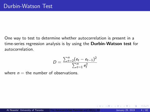
Durbin-Watson Test
One way to test to determine whether autocorrelation is present in atime-series regression analysis is by using the Durbin-Watson test forautocorrelation.
D =
∑nt=2(et − et−1)2∑n
t=1 e2t
where n = the number of observations.
Al Nosedal University of Toronto The Autocorrelation Function and AR(1), AR(2) Models January 29, 2019 4 / 82

Durbin-Watson Test (cont.)
The range of values of D is 0 ≤ D ≤ 4 where small values of D (D < 2)indicate a positive first-order autocorrelation and large values of D(D > 2) imply a negative first-order autocorrelation. Positive first-orderautocorrelation is a common occurrence in business and economic timeseries. The null hypothesis for this test is that there is no autocorrelation.A one-tailed test is used:
H0 : ρ = 0 vs Ha : ρ > 0
In the Durbin-Watson test, D is the observed value of the Durbin-Watsonstatistic using the residuals from the regression analysis. Our Tables aredesigned to test for positive first-order autocorrelation by providing valuesof dL and dU for a variety of values of n and k and for α = 0.01 andα = 0.05.
Al Nosedal University of Toronto The Autocorrelation Function and AR(1), AR(2) Models January 29, 2019 5 / 82
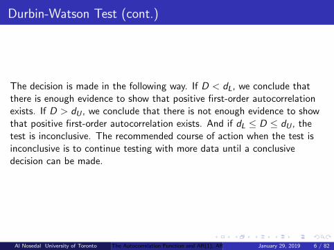
Durbin-Watson Test (cont.)
The decision is made in the following way. If D < dL, we conclude thatthere is enough evidence to show that positive first-order autocorrelationexists. If D > dU , we conclude that there is not enough evidence to showthat positive first-order autocorrelation exists. And if dL ≤ D ≤ dU , thetest is inconclusive. The recommended course of action when the test isinconclusive is to continue testing with more data until a conclusivedecision can be made.
Al Nosedal University of Toronto The Autocorrelation Function and AR(1), AR(2) Models January 29, 2019 6 / 82

Durbin-Watson Test (cont.)
To test for negative first-order autocorrelation, we change the criticalvalues. If D > 4− dL, we conclude that negative first-orderautocorrelation exists. If D < 4− dU , we conclude that there is notenough evidence to show that negative first-order autocorrelation exists. If4− du ≤ D ≤ 4− dL, the test is inconclusive.
Al Nosedal University of Toronto The Autocorrelation Function and AR(1), AR(2) Models January 29, 2019 7 / 82
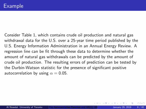
Example
Consider Table 1, which contains crude oil production and natural gaswithdrawal data for the U.S. over a 25-year time period published by theU.S. Energy Information Administration in an Annual Energy Review. Aregression line can be fit through these data to determine whether theamount of natural gas withdrawals can be predicted by the amount ofcrude oil production. The resulting errors of prediction can be tested bythe Durbin-Watson statistic for the presence of significant positiveautocorrelation by using α = 0.05.
Al Nosedal University of Toronto The Autocorrelation Function and AR(1), AR(2) Models January 29, 2019 8 / 82

Table 1
Year Crude Oil Natural GasProduction (1000s) Withdrawals (1000s)
1 8.597 17.5732 8.572 17.3373 8.649 15.8094 8.688 14.1535 8.879 15.5136 8.971 14.5357 8.680 14.1548 8.349 14.8079 8.140 15.467
10 7.613 15.70911 7.355 16.05412 7.417 16.01813 7.171 16.165
Al Nosedal University of Toronto The Autocorrelation Function and AR(1), AR(2) Models January 29, 2019 9 / 82
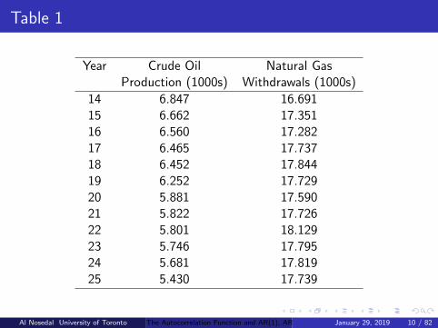
Table 1
Year Crude Oil Natural GasProduction (1000s) Withdrawals (1000s)
14 6.847 16.69115 6.662 17.35116 6.560 17.28217 6.465 17.73718 6.452 17.84419 6.252 17.72920 5.881 17.59021 5.822 17.72622 5.801 18.12923 5.746 17.79524 5.681 17.81925 5.430 17.739
Al Nosedal University of Toronto The Autocorrelation Function and AR(1), AR(2) Models January 29, 2019 10 / 82

R Code (entering data)
# explanatory variable;
# oil= crude oil production;
oil=c( 8.597,8.572,8.649,8.688,
8.879,8.971,8.680,8.349,
8.140,7.613,7.355,7.417,
7.171,6.847,6.662,6.560,
6.465,6.452,6.252,5.881,
5.822,5.801,5.746,5.681,
5.430);
Al Nosedal University of Toronto The Autocorrelation Function and AR(1), AR(2) Models January 29, 2019 11 / 82
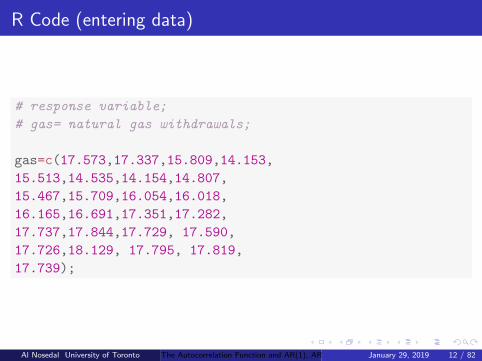
R Code (entering data)
# response variable;
# gas= natural gas withdrawals;
gas=c(17.573,17.337,15.809,14.153,
15.513,14.535,14.154,14.807,
15.467,15.709,16.054,16.018,
16.165,16.691,17.351,17.282,
17.737,17.844,17.729, 17.590,
17.726,18.129, 17.795, 17.819,
17.739);
Al Nosedal University of Toronto The Autocorrelation Function and AR(1), AR(2) Models January 29, 2019 12 / 82

R Code (fitting linear model)
lin.mod=lm(gas~oil);
names(lin.mod);
Al Nosedal University of Toronto The Autocorrelation Function and AR(1), AR(2) Models January 29, 2019 13 / 82
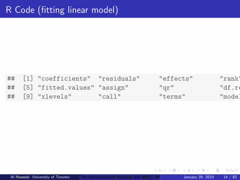
R Code (fitting linear model)
## [1] "coefficients" "residuals" "effects" "rank"
## [5] "fitted.values" "assign" "qr" "df.residual"
## [9] "xlevels" "call" "terms" "model"
Al Nosedal University of Toronto The Autocorrelation Function and AR(1), AR(2) Models January 29, 2019 14 / 82

R Code (finding residuals)
round(lin.mod$res,4);
# round will round residual using 4 decimal places;
Al Nosedal University of Toronto The Autocorrelation Function and AR(1), AR(2) Models January 29, 2019 15 / 82

R Code (finding residuals)
## 1 2 3 4 5 6 7 8 9
## 2.1492 1.8920 0.4295 -1.1933 0.3291 -0.5706 -1.1991 -0.8277 -0.3455
## 10 11 12 13 14 15 16 17 18
## -0.5518 -0.4263 -0.4096 -0.4718 -0.2215 0.2811 0.1254 0.4996 0.5955
## 19 20 21 22 23 24 25
## 0.3104 -0.1443 -0.0584 0.3267 -0.0541 -0.0854 -0.3789
Al Nosedal University of Toronto The Autocorrelation Function and AR(1), AR(2) Models January 29, 2019 16 / 82
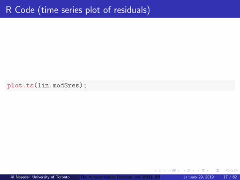
R Code (time series plot of residuals)
plot.ts(lin.mod$res);
Al Nosedal University of Toronto The Autocorrelation Function and AR(1), AR(2) Models January 29, 2019 17 / 82

R Code (time series plot of residuals)
Time
lin.m
od$r
es
5 10 15 20 25
−1.
00.
52.
0
Al Nosedal University of Toronto The Autocorrelation Function and AR(1), AR(2) Models January 29, 2019 18 / 82

R Code (installing library)
install.packages("lmtest");
Al Nosedal University of Toronto The Autocorrelation Function and AR(1), AR(2) Models January 29, 2019 19 / 82
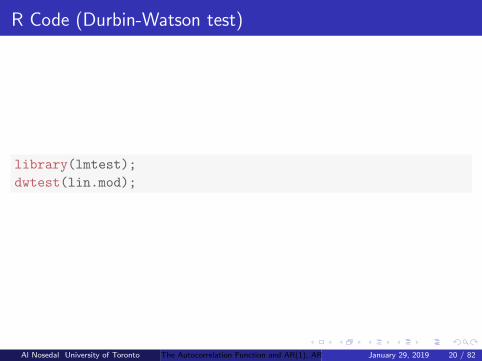
R Code (Durbin-Watson test)
library(lmtest);
dwtest(lin.mod);
Al Nosedal University of Toronto The Autocorrelation Function and AR(1), AR(2) Models January 29, 2019 20 / 82

R Code (installing library)
##
## Durbin-Watson test
##
## data: lin.mod
## DW = 0.68731, p-value = 2.256e-05
## alternative hypothesis: true autocorrelation is greater than 0
Al Nosedal University of Toronto The Autocorrelation Function and AR(1), AR(2) Models January 29, 2019 21 / 82

Using table
Because we used a simple linear regression, the value of k = 1. The samplesize, n, is 25, and α = 0.05. The critical values in our Table A− 2 are:
dL = 1.288 and dU = 1.454
Because the computed D statistic, 0.6873, is less than the value ofdL = 1.288, the null hypothesis is rejected. We have evidence that apositive autocorrelation is present in this example.
Al Nosedal University of Toronto The Autocorrelation Function and AR(1), AR(2) Models January 29, 2019 22 / 82
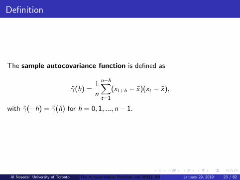
Definition
The sample autocovariance function is defined as
γ̂(h) =1
n
n−h∑t=1
(xt+h − x̄)(xt − x̄),
with γ̂(−h) = γ̂(h) for h = 0, 1, ..., n − 1.
Al Nosedal University of Toronto The Autocorrelation Function and AR(1), AR(2) Models January 29, 2019 23 / 82

Definition
The sample autocorrelation function is defined as
ρ̂(h) =γ̂(h)
γ̂(0).
Al Nosedal University of Toronto The Autocorrelation Function and AR(1), AR(2) Models January 29, 2019 24 / 82

Toy Example
To understand autocorrelation it is first necessary to understand what itmeans to lag a time series.Y (t) = Yt =(3,4,5,6,7,8,9,10,11,12)
Y lagged 1 = Y (t − 1) = Yt−1 =(*,3,4,5,6,7,8,9,10,11)
Al Nosedal University of Toronto The Autocorrelation Function and AR(1), AR(2) Models January 29, 2019 25 / 82

Toy Example (cont.)
Find the sample autocorrelation at lag 1 for the following time series:Y (t) = (3, 4, 5, 6, 7, 8, 9, 10, 11, 12).Answer.ρ̂(1) = 0.7
Al Nosedal University of Toronto The Autocorrelation Function and AR(1), AR(2) Models January 29, 2019 26 / 82
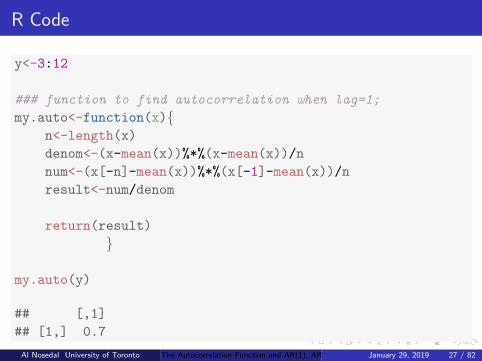
R Code
y<-3:12
### function to find autocorrelation when lag=1;
my.auto<-function(x){n<-length(x)
denom<-(x-mean(x))%*%(x-mean(x))/n
num<-(x[-n]-mean(x))%*%(x[-1]-mean(x))/n
result<-num/denom
return(result)
}
my.auto(y)
## [,1]
## [1,] 0.7
Al Nosedal University of Toronto The Autocorrelation Function and AR(1), AR(2) Models January 29, 2019 27 / 82

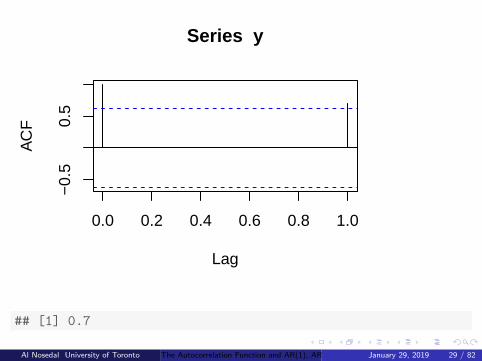
An easier way of finding autocorrelations
Using R, we can easily find the autocorrelation at any lag k.
y<-3:12
auto.lag1<-acf(y,lag=1)$acf[2]
auto.lag1
Al Nosedal University of Toronto The Autocorrelation Function and AR(1), AR(2) Models January 29, 2019 28 / 82
0.0 0.2 0.4 0.6 0.8 1.0
−0.
50.
5
Lag
AC
FSeries y
## [1] 0.7
Al Nosedal University of Toronto The Autocorrelation Function and AR(1), AR(2) Models January 29, 2019 29 / 82
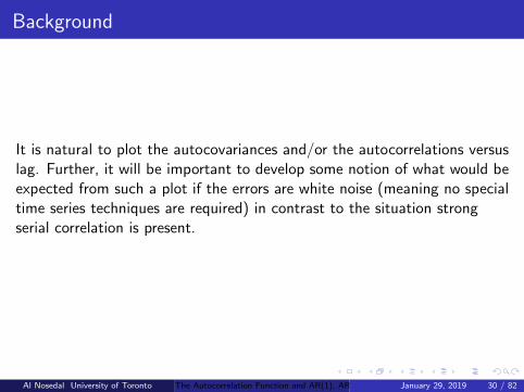
Background
It is natural to plot the autocovariances and/or the autocorrelations versuslag. Further, it will be important to develop some notion of what would beexpected from such a plot if the errors are white noise (meaning no specialtime series techniques are required) in contrast to the situation strongserial correlation is present.
Al Nosedal University of Toronto The Autocorrelation Function and AR(1), AR(2) Models January 29, 2019 30 / 82
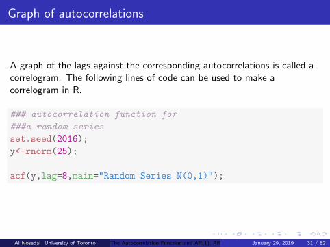
Graph of autocorrelations
A graph of the lags against the corresponding autocorrelations is called acorrelogram. The following lines of code can be used to make acorrelogram in R.
### autocorrelation function for
###a random series
set.seed(2016);
y<-rnorm(25);
acf(y,lag=8,main="Random Series N(0,1)");
Al Nosedal University of Toronto The Autocorrelation Function and AR(1), AR(2) Models January 29, 2019 31 / 82
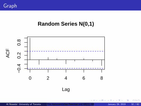
Graph
0 2 4 6 8
−0.
40.
20.
8
Lag
AC
F
Random Series N(0,1)
Al Nosedal University of Toronto The Autocorrelation Function and AR(1), AR(2) Models January 29, 2019 32 / 82

The AR(1) Model Autocorrelation and Autocovariance
For the AR(1) model, xj = a1xj−1 + wj , xj = a21xj−2 + a1wj−1 + wj , and in
general xj = ak1xj−k +∑k
t=1 at−11 wj−t+1.
Furthermore γ(1) = E (xjxj−1) = E ([a1xj−1 + wk ]xj−1) = a1σ2AR = a1γ(0).
Al Nosedal University of Toronto The Autocorrelation Function and AR(1), AR(2) Models January 29, 2019 33 / 82

The AR(1) Model Autocorrelation and Autocovariance
More generally,γ(k) = E (xjxj−k) = E ([ak1xj−k +
∑kt=1 a
t−11 wj−t+1]xj−k) = ak1γ(0).
So, in general ρ(k) = a|k|1 .
Al Nosedal University of Toronto The Autocorrelation Function and AR(1), AR(2) Models January 29, 2019 34 / 82
The AR(1) Model Autocorrelation and Autocovariance
For AR(1), the relationship of variance in the series to variance in whitenoise isσ2AR = E (xjxj) = E ([a1xj−1 + wj ][a1xj−1 + wj ]) = a21σ
2AR + σ2w , so
σ2AR = σ2w
1−a21.
Al Nosedal University of Toronto The Autocorrelation Function and AR(1), AR(2) Models January 29, 2019 35 / 82

The Stationary AR(1) is an MA model of infinite order
Here we introduce the fundamental duality between AR and MA models.We can keep going backward in time using the first-order autoregressivemodel:xt = a1xt−1 + wt
xt = a1(a1xt−2 + wt−1) + wt
or xt = a21xt−2 + (a1wt−1 + wt)= a21(a1xt−3 + wt−2) + (a1wt−1 + wt)= a31xt−3 + a21wt−2 + a1wt−1 + wt
Al Nosedal University of Toronto The Autocorrelation Function and AR(1), AR(2) Models January 29, 2019 36 / 82

The Stationary AR(1) is an MA model of infinite order
Continuing back to minus infinity we would get
xt = wt + a1wt−1 + a21wt−2 + a31xt−3 + ...
which makes sense if it is the case that ak1 → 0 as k →∞ rapidly enoughfor the series to converge to a finite limit. This is our stationary condition.
Al Nosedal University of Toronto The Autocorrelation Function and AR(1), AR(2) Models January 29, 2019 37 / 82
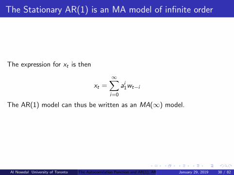
The Stationary AR(1) is an MA model of infinite order
The expression for xt is then
xt =∞∑i=0
ai1wt−i
The AR(1) model can thus be written as an MA(∞) model.
Al Nosedal University of Toronto The Autocorrelation Function and AR(1), AR(2) Models January 29, 2019 38 / 82

The AR(1) process is not always stationary
The variance of the AR(1) process is given by
σ2AR = Var(xt) = Var
( ∞∑i=0
ai1wt−i
)
σ2AR = Var(xt) = σ2w (1 + a21 + (a21)2 + (a21)3 + (a21)4 + ...)
If a1 = 1 or if a1 is larger, this variance will increase without bound.
Al Nosedal University of Toronto The Autocorrelation Function and AR(1), AR(2) Models January 29, 2019 39 / 82
The Yule-Walker equations
The development of these useful equations is not difficult. Write thegeneral AR(p) model as
xt = a1xt−1 + a2xt−2 + ...+ apxt−p + wt
where we assume that xt is a zero-mean process (or that the mean hasbeen subtracted) and that wt is a white-noise process and thatE (wtxt−k) = 0 for k > 0. Once again, compute γ(k):
γ(k) = E (xtxt−k)
Al Nosedal University of Toronto The Autocorrelation Function and AR(1), AR(2) Models January 29, 2019 40 / 82
The Yule-Walker equations
γ(k) = E (xtxt−k) = E [(a1xt−1 + a2xt−2 + ...+ apxt−p + wt)xt−k ]γ(k) = E (xtxt−k) =a1E [xt−1xt−k ] + a2E [xt−2xt−k ] + ...+ apE [xt−pxt−k ] + E [wtxt−k ]
Al Nosedal University of Toronto The Autocorrelation Function and AR(1), AR(2) Models January 29, 2019 41 / 82
The Yule-Walker equations
From the definition of the autocovariance γ(k) of a stationary process, itis a function only of the lag between observations. Thus,γ(k) = E (xtxt−k) = E (xt+sxt+s−k).We can use this fact to simplify γ(k) = E (xtxt−k) =a1E [xt−1xt−k ] + a2E [xt−2xt−k ] + ...+ apE [xt−pxt−k ] +E [wtxt−k ] to obtain
γ(k) = a1γ(k − 1) + a2γ(k − 2) + ...+ apγ(k − p) + E (wtxt−k)
Al Nosedal University of Toronto The Autocorrelation Function and AR(1), AR(2) Models January 29, 2019 42 / 82
The Yule-Walker equations
For k > 0 we know that the last term is zero.
γ(k) = a1γ(k − 1) + a2γ(k − 2) + ...+ apγ(k − p).
If we divide by the variance of the series γ(0) = σ2AR and recall the
definition of the autocorrelation ρ(k) = γ(k)γ(0) , we obtain the Yule-Walker
equations
ρ(k) = a1ρ(k − 1) + a2ρ(k − 2) + ...+ apρ(k − p), k > 0.
Al Nosedal University of Toronto The Autocorrelation Function and AR(1), AR(2) Models January 29, 2019 43 / 82
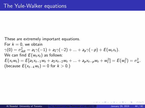
The Yule-Walker equations
These are extremely important equations.For k = 0, we obtainγ(0) = σ2AR = a1γ(−1) + a2γ(−2) + ...+ apγ(−p) + E (wtxt).We can find E (wtxt) as follows:E (xtwt) = E [a1xt−1wt + a2xt−2wt + ...+ apxt−pwt + w2
t ] = E (w2t ) = σ2w .
(because E (xt−kwt) = 0 for k > 0.)
Al Nosedal University of Toronto The Autocorrelation Function and AR(1), AR(2) Models January 29, 2019 44 / 82
The Yule-Walker equations
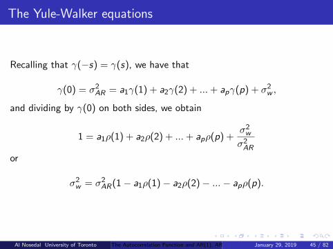
Recalling that γ(−s) = γ(s), we have that
γ(0) = σ2AR = a1γ(1) + a2γ(2) + ...+ apγ(p) + σ2w ,
and dividing by γ(0) on both sides, we obtain
1 = a1ρ(1) + a2ρ(2) + ...+ apρ(p) +σ2wσ2AR
or
σ2w = σ2AR(1− a1ρ(1)− a2ρ(2)− ...− apρ(p).
Al Nosedal University of Toronto The Autocorrelation Function and AR(1), AR(2) Models January 29, 2019 45 / 82
Why are Yule-Walker equations so important?
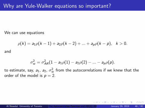
We can use equations
ρ(k) = a1ρ(k − 1) + a2ρ(k − 2) + ...+ apρ(k − p), k > 0.
and
σ2w = σ2AR(1− a1ρ(1)− a2ρ(2)− ...− apρ(p).
to estimate, say, a1, a2, σ2w from the autocorrelations if we knew that theorder of the model is p = 2.
Al Nosedal University of Toronto The Autocorrelation Function and AR(1), AR(2) Models January 29, 2019 46 / 82

AR(2) Process
This process is defined by
xt = a1xt−1 + a2xt−2 + wt .
It can be shown that
a1 =ρ(1)[1− ρ(2)]
1− ρ(1)2
a2 =ρ(2)− ρ(1)2
1− ρ(1)2
Al Nosedal University of Toronto The Autocorrelation Function and AR(1), AR(2) Models January 29, 2019 47 / 82
Stationarity conditions for an AR(2) process
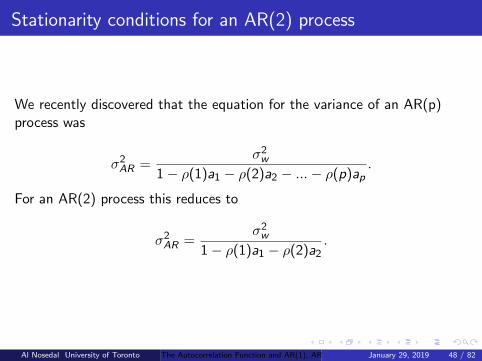
We recently discovered that the equation for the variance of an AR(p)process was
σ2AR =σ2w
1− ρ(1)a1 − ρ(2)a2 − ...− ρ(p)ap.
For an AR(2) process this reduces to
σ2AR =σ2w
1− ρ(1)a1 − ρ(2)a2.
Al Nosedal University of Toronto The Autocorrelation Function and AR(1), AR(2) Models January 29, 2019 48 / 82
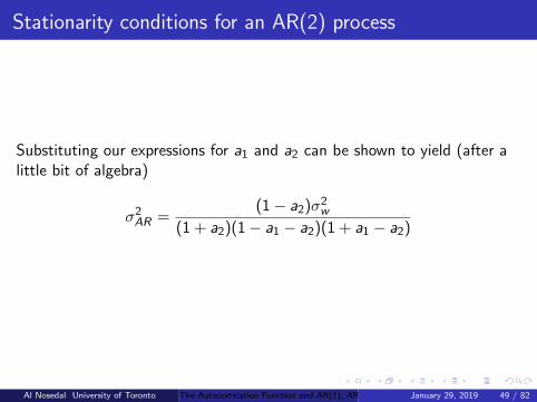
Stationarity conditions for an AR(2) process
Substituting our expressions for a1 and a2 can be shown to yield (after alittle bit of algebra)
σ2AR =(1− a2)σ2w
(1 + a2)(1− a1 − a2)(1 + a1 − a2)
Al Nosedal University of Toronto The Autocorrelation Function and AR(1), AR(2) Models January 29, 2019 49 / 82

Stationarity conditions for an AR(2) process
Using the facts that autocorrelations must be less than 1, and each factorin the denominator and numerator must be positive, we can derive theconditions−1 < a2 < 1a2 + a1 < 1a2 − a1 < 1The inequalities define the stationarity region for AR(2).
Al Nosedal University of Toronto The Autocorrelation Function and AR(1), AR(2) Models January 29, 2019 50 / 82

Scatterplot to Illustrate the AR(1) Model
The model AR(1) is about the correlation between an error and theprevious error. First consider white noise. In this case there should be nocorrelation between the errors and the shifted errors.On the other hand, consider AR(1) errors with a1 = 0.7.
Al Nosedal University of Toronto The Autocorrelation Function and AR(1), AR(2) Models January 29, 2019 51 / 82
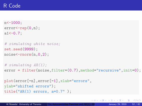
R Code
n<-1000;
error<-rep(0,n);
a1<-0.7;
# simulating white noise;
set.seed(9999);
noise<-rnorm(n,0,2);
# simulating AR(1);
error = filter(noise,filter=(0.7),method="recursive",init=0);
plot(error[-n],error[-1],xlab="errors",
ylab="shifted errors");
title("AR(1) errors, a=0.7" );
Al Nosedal University of Toronto The Autocorrelation Function and AR(1), AR(2) Models January 29, 2019 52 / 82

Scatterplot
● ●
●
● ●
●●
●●
●●
●●●●●
●●
● ●●●
●●●
●
● ●●●
●●
●● ●●
●
●●
● ● ●
●●
● ●●●●
● ●
● ●
●
●●
●●
●●
●
●● ●●
●●●
● ●●
●
● ●●
●
●●
●● ●
●
●●●●
●●
●●
●
●●●
●
●
●●
●
●● ●●
●●●
●●
●●●
● ●●
●●●
●●●● ●
●●
●●
● ●
●●●
●
●
●●
●
●
●●●●●
●
●●●●
● ●● ●●
● ●●
●● ●●
●●
●●●
●
●●●●
● ●●
●●
●
●●
●
●
●●●
●
●●● ●●
● ●●
●●●●●●
●
●
●
●●
●
● ●●
●●
●●
●
●●
●
● ●●
●●
●
● ●●
●
●
●
●●●
●●
●
●●
●
●
●
●
●
●
● ●
●●
●●●●
●● ●
●●●
●
●●
●
●
●
●
●
●
● ●●
●
●●
●●●● ●●
●●
●
●
●●
● ● ●●
●● ●●
● ●
●●
●● ●
●●
●
●
●●
●
●●● ●
●●
●
●●
●
●●
●●
●
●
●
●● ●
●
●
●
● ●●●●
●●
●●
●●●
● ●●
●
●
●
●
●●●●
● ●
●● ●
●●
●●
●●
●
●
●●
●
●●
●
● ●●●● ●
●
●
●●●
●
● ●●●
●
●
●●
●
●
●●●
●
● ●● ●
●●
●●
●●●●
●●
●●
●●
●
●
●●●
● ●●
●●●
●●●
●●
●●
● ●
●●●
● ●●●
●●
● ●●●●
●
●●
●● ●
●
●●●
●
●
●●
●
●●●
●●
●●
●●
●
●●
●●
● ●●
●●
●
● ●
●●●●
●
● ●●
● ●●
●
●●
●
●●
●●
●●●
● ●●
●● ●
●●●
●●●
●
●
●● ●
●
●●
●●
●
●●●●●●●
●●
●
●
●●
●●●●
●● ●●
●● ●
●
●●●●●●
● ●
●●
●●
●● ●
●● ●
●●
●
● ●●
●●
● ●●
●●● ●●
●●
●●
●●
●●
●●● ●●●
●
●
●●
●
●●● ●
● ●
●
●● ●
●
●●● ●
●
●●●
●● ●●●
●●
● ●●●
●
●
●●
●●
● ●●
● ●●
●●●● ●
●
●●
● ●
●●
●
●●●
● ●● ●
● ●●
●● ●●●●
●●
●●
●
●
●●
● ●●
●●
●●● ●
●●●
● ●● ●
●●●
● ●
●
●
●● ●
●
●
●●
●
●
●
●
●
● ●●
●●
●
●●●●
●●
●●
●●●●
●● ●●●
●
●
● ●●●●
●●
●●
● ●●●
●●●
●
●●
●
● ●● ●
●●●
●● ●
●●
●●
●●
● ●●●
●●
●
●●●
●●
●
●●
●●
●●
●●●
●
●● ●●
●
●●
●● ●
●
●●
●●
●●
●●
●●
●
●
●
●
●
●
●
●●
●●
●●
●
● ●●●●
●●
●
●●
●
●●●
●●
● ●
●●●●● ●●
●
●
●
●●
●
●●
●●
● ●●●●
●●●●
●●●
●●
●
●
● ●
●
●●
●
●
●
●●
●●
●●
●
●● ●●
● ●
●
● ●●
● ●●
●
●
●
●●●
●●
●●●●
●● ●●●
● ●
●●●●●
●●●
●
●
●
●●
●
●●
●●
●
●
●
●
●●
● ●●
●● ●●●
●
●●
● ●●●●●●●
●● ●
●●●
● ●●●
●●
●
●●
●●
●
●
−5 0 5 10
−5
05
10
errors
shift
ed e
rror
s
AR(1) errors, a=0.7
Al Nosedal University of Toronto The Autocorrelation Function and AR(1), AR(2) Models January 29, 2019 53 / 82

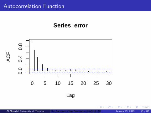
Autocorrelation Function
acf(error);
Al Nosedal University of Toronto The Autocorrelation Function and AR(1), AR(2) Models January 29, 2019 54 / 82
Autocorrelation Function
0 5 10 15 20 25 30
0.0
0.4
0.8
Lag
AC
F
Series error
Al Nosedal University of Toronto The Autocorrelation Function and AR(1), AR(2) Models January 29, 2019 55 / 82

Based on the formulas already derived and the choice used in the code(a1 = 0.7):ρ(0) = 1 by definition
ρ(1) = a|1|1 = 0.7
ρ(2) = a|2|1 = 0.49
ρ(3) = a|3|1 = 0.343
ρ(4) = a|4|1 = 0.2401
Al Nosedal University of Toronto The Autocorrelation Function and AR(1), AR(2) Models January 29, 2019 56 / 82

R Code
acf(error,plot=FALSE)[0:4];
##
## Autocorrelations of series 'error', by lag
##
## 0 1 2 3 4
## 1.000 0.690 0.461 0.319 0.216
Al Nosedal University of Toronto The Autocorrelation Function and AR(1), AR(2) Models January 29, 2019 57 / 82

Examples of Stable and Unstable AR(1) Models
Consider the following three cases of AR(1) data:
1. a1 = −0.9
2. a1 = 0.5
3. a1 = 1.01
Al Nosedal University of Toronto The Autocorrelation Function and AR(1), AR(2) Models January 29, 2019 58 / 82

Case 1
n<-100;
error<-rep(0,n);
a1<- -0.9;
set.seed(9999);
noise<-rnorm(n,0,2);
error <- filter(noise,filter=(a1),method="recursive",
init=0);
plot.ts(error,main="a = -0.9, n =100");
acf(error);
Al Nosedal University of Toronto The Autocorrelation Function and AR(1), AR(2) Models January 29, 2019 59 / 82

Case 1. Time Series
a = −0.9, n =100
Time
erro
r
0 20 40 60 80 100
−10
05
Al Nosedal University of Toronto The Autocorrelation Function and AR(1), AR(2) Models January 29, 2019 60 / 82
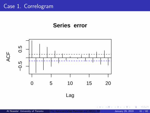
Case 1. Correlogram
0 5 10 15 20
−0.
50.
5
Lag
AC
F
Series error
Al Nosedal University of Toronto The Autocorrelation Function and AR(1), AR(2) Models January 29, 2019 61 / 82

Case 2
n<-100;
error<-rep(0,n);
a1<- 0.5;
set.seed(9999);
noise<-rnorm(n,0,2);
error <- filter(noise,filter=(a1),method="recursive",
init=0);
plot.ts(error,main="a = 0.5, n =100");
acf(error);
Al Nosedal University of Toronto The Autocorrelation Function and AR(1), AR(2) Models January 29, 2019 62 / 82
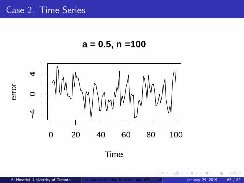
Case 2. Time Series
a = 0.5, n =100
Time
erro
r
0 20 40 60 80 100
−4
04
Al Nosedal University of Toronto The Autocorrelation Function and AR(1), AR(2) Models January 29, 2019 63 / 82

Case 2. Correlogram
0 5 10 15 20
−0.
20.
41.
0
Lag
AC
F
Series error
Al Nosedal University of Toronto The Autocorrelation Function and AR(1), AR(2) Models January 29, 2019 64 / 82
Case 3
n<-100;
error<-rep(0,n);
a1<- 1.1;
set.seed(9999);
noise<-rnorm(n,0,2);
error <- filter(noise,filter=(a1),method="recursive",
init=0);
plot.ts(error,main="a = 1.1, n =100");
acf(error);
Al Nosedal University of Toronto The Autocorrelation Function and AR(1), AR(2) Models January 29, 2019 65 / 82
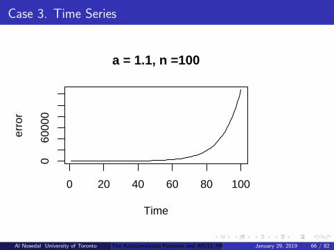
Case 3. Time Series
a = 1.1, n =100
Time
erro
r
0 20 40 60 80 100
060
000
Al Nosedal University of Toronto The Autocorrelation Function and AR(1), AR(2) Models January 29, 2019 66 / 82
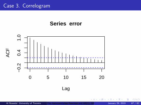
Case 3. Correlogram
0 5 10 15 20
−0.
20.
41.
0
Lag
AC
F
Series error
Al Nosedal University of Toronto The Autocorrelation Function and AR(1), AR(2) Models January 29, 2019 67 / 82
The AR(2) Model Autocorrelation and Autocovariance
The model is:
xt = a1xt−1 + a2xt−2 + wt ,
and the autocovariances can be characterized with recursive relationships.
Al Nosedal University of Toronto The Autocorrelation Function and AR(1), AR(2) Models January 29, 2019 68 / 82

γ(1) and ρ(1)
γ(1) = E (xjxj−1) = E ([a1xj−1 + a2xj−2 + wj ]xj−1) = a1γ(0) + a2γ(1), soit is easy to see that ρ(1) = a1
1−a2 .
Al Nosedal University of Toronto The Autocorrelation Function and AR(1), AR(2) Models January 29, 2019 69 / 82

ρ(2) and ρ(3)
Doing something similar,
ρ(2) =a21
(1− a2)+ a2
and
ρ(3) =a31 + a1a2(1− a2)
+ a1a2.
Al Nosedal University of Toronto The Autocorrelation Function and AR(1), AR(2) Models January 29, 2019 70 / 82
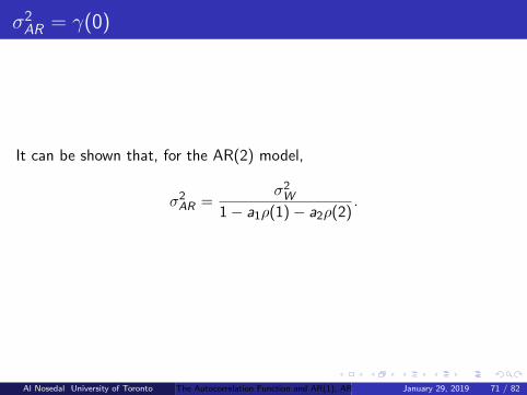
σ2AR = γ(0)
It can be shown that, for the AR(2) model,
σ2AR =σ2W
1− a1ρ(1)− a2ρ(2).
Al Nosedal University of Toronto The Autocorrelation Function and AR(1), AR(2) Models January 29, 2019 71 / 82
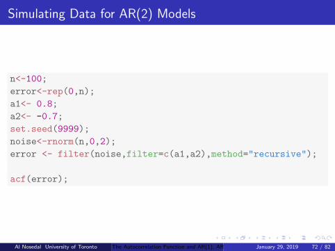
Simulating Data for AR(2) Models
n<-100;
error<-rep(0,n);
a1<- 0.8;
a2<- -0.7;
set.seed(9999);
noise<-rnorm(n,0,2);
error <- filter(noise,filter=c(a1,a2),method="recursive");
acf(error);
Al Nosedal University of Toronto The Autocorrelation Function and AR(1), AR(2) Models January 29, 2019 72 / 82

Correlogram
0 5 10 15 20
−0.
50.
5
Lag
AC
F
Series error
Al Nosedal University of Toronto The Autocorrelation Function and AR(1), AR(2) Models January 29, 2019 73 / 82

Autocorrelations
Based on the formulas already derived and the choices used in the code(a1 = 0.8, a2 = 0.7):ρ(0) = 1, ρ(1) = a1
1−a2 = 0.81.7 ≈ 0.4706,
ρ(2) = a1ρ(1) + a2ρ(0) ≈ 0.8(0.4706)− 0.7(1) ≈ −0.3235,ρ(3) = a1ρ(2) + a2ρ(1) ≈ 0.8(−0.3235)− 0.7(0.4706) ≈ −0.5882, etc.
Al Nosedal University of Toronto The Autocorrelation Function and AR(1), AR(2) Models January 29, 2019 74 / 82

Stable and Unstable AR(2) Models
Recall the AR(2) process is stationary when:i) a1 + a2 < 1,ii) a2 − a1 < 1, andiii) |a2| < 1.
Al Nosedal University of Toronto The Autocorrelation Function and AR(1), AR(2) Models January 29, 2019 75 / 82
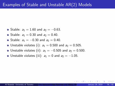
Examples of Stable and Unstable AR(2) Models
Stable: a1 = 1.60 and a2 = −0.63.
Stable: a1 = 0.30 and a2 = 0.40.
Stable: a1 = −0.30 and a2 = 0.40.
Unstable violates (i): a1 = 0.500 and a2 = 0.505.
Unstable violates (ii): a1 = −0.505 and a2 = 0.500.
Unstable violates (iii): a1 = 0 and a2 = −1.05.
Al Nosedal University of Toronto The Autocorrelation Function and AR(1), AR(2) Models January 29, 2019 76 / 82

Unstable case a1 = 0.500 and a2 = 0.505.
n<-100;
error<-rep(0,n);
a1<- 0.500;
a2<- 0.505;
set.seed(9);
noise<-rnorm(n,0,2);
error <- filter(noise,filter=c(a1,a2),method="recursive");
plot.ts(error,main="a1 = 0.5 and a2=-0.505, n =100");
Al Nosedal University of Toronto The Autocorrelation Function and AR(1), AR(2) Models January 29, 2019 77 / 82

Unstable case a1 = 0.500 and a2 = 0.505.
a1 = 0.5 and a2=0.505, n =100
Time
erro
r
0 20 40 60 80 100
−10
−4
04
Al Nosedal University of Toronto The Autocorrelation Function and AR(1), AR(2) Models January 29, 2019 78 / 82

Unstable case a1 = −0.505 and a2 = 0.500.
n<-100;
error<-rep(0,n);
a1<- - 0.505;
a2<- 0.500;
set.seed(9);
noise<-rnorm(n,0,2);
error <- filter(noise,filter=c(a1,a2),method="recursive");
plot.ts(error,main="a1 = - 0.505 and a2=0.500, n =100");
Al Nosedal University of Toronto The Autocorrelation Function and AR(1), AR(2) Models January 29, 2019 79 / 82

Unstable case a1 = −0.505 and a2 = 0.500.
a1 = − 0.505 and a2=0.500, n =100
Time
erro
r
0 20 40 60 80 100
−30
020
Al Nosedal University of Toronto The Autocorrelation Function and AR(1), AR(2) Models January 29, 2019 80 / 82
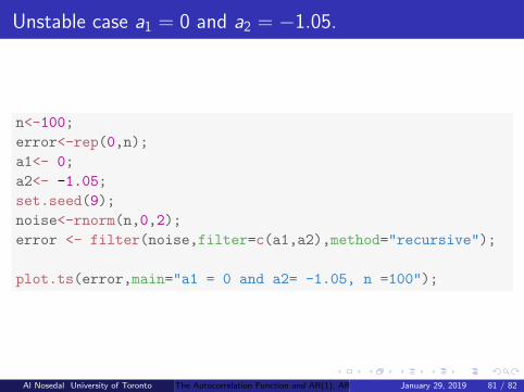
Unstable case a1 = 0 and a2 = −1.05.
n<-100;
error<-rep(0,n);
a1<- 0;
a2<- -1.05;
set.seed(9);
noise<-rnorm(n,0,2);
error <- filter(noise,filter=c(a1,a2),method="recursive");
plot.ts(error,main="a1 = 0 and a2= -1.05, n =100");
Al Nosedal University of Toronto The Autocorrelation Function and AR(1), AR(2) Models January 29, 2019 81 / 82

Unstable case a1 = 0 and a2 = −1.05.
a1 = 0 and a2= −1.05, n =100
Time
erro
r
0 20 40 60 80 100
−50
050
Al Nosedal University of Toronto The Autocorrelation Function and AR(1), AR(2) Models January 29, 2019 82 / 82