Correlation and Autocorrelation

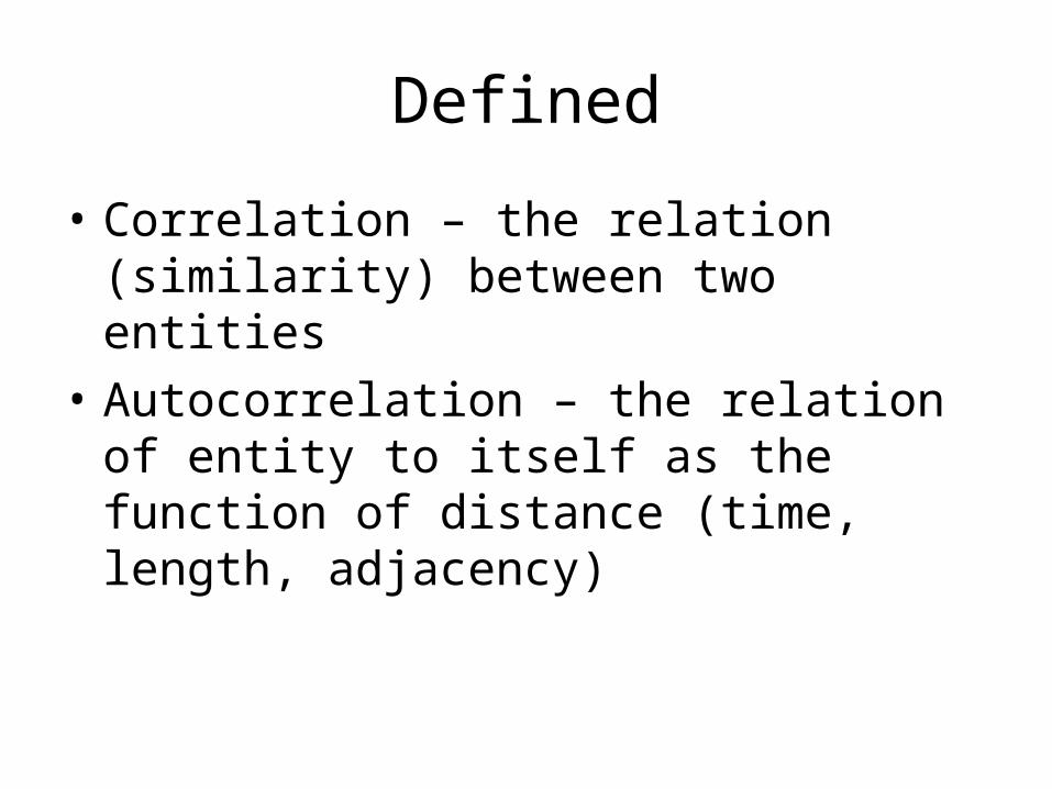
Defined

• Correlation – the relation (similarity) between two entities

• Autocorrelation – the relation of entity to itself as the function of distance (time, length, adjacency)

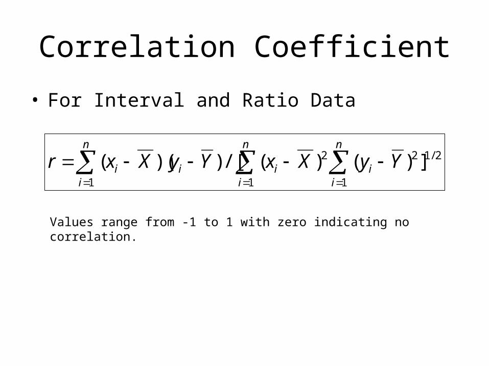
Correlation Coefficient

• For Interval and Ratio Data

2/12

1

2

11

])()(/[))((

n

ii

n

iii

n

ii YyXxYyXxr

Values range from -1 to 1 with zero indicating no correlation.

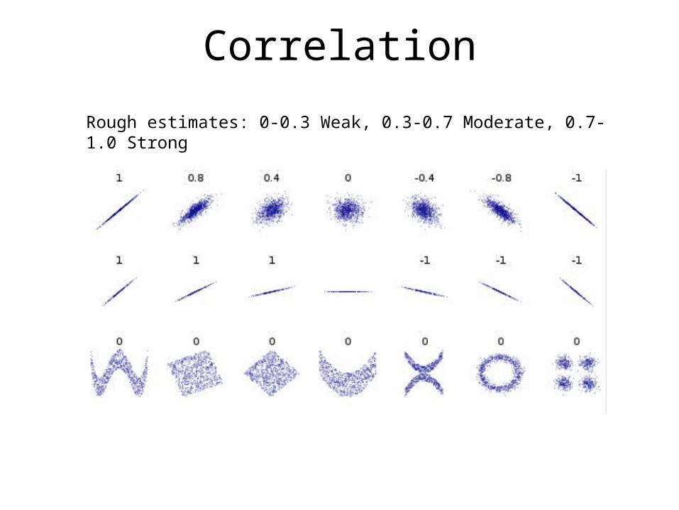
Correlation

Rough estimates: 0-0.3 Weak, 0.3-0.7 Moderate, 0.7-1.0 Strong

Test for Correlation

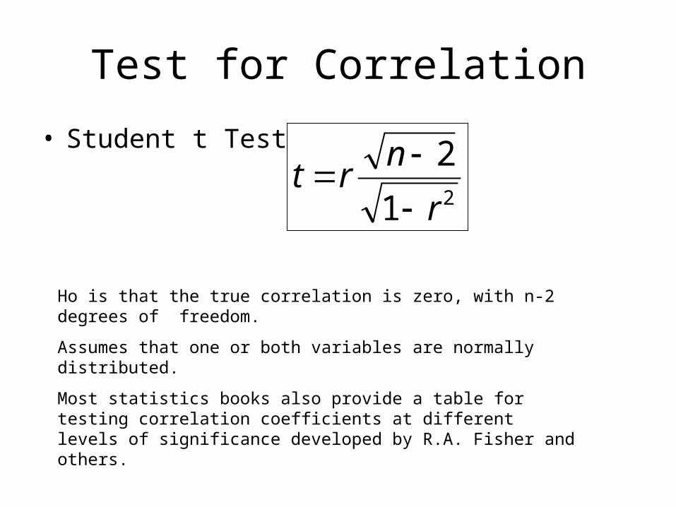
• Student t Test

21

2

r

nrt

Ho is that the true correlation is zero, with n-2 degrees of freedom.

Assumes that one or both variables are normally distributed.

Most statistics books also provide a table for testing correlation coefficients at different levels of significance developed by R.A. Fisher and others.

Correlation of Surfaces

• Cell by Cell comparison using rasters.• For other data structures you usually

correlation on a set of point measurements that obtain a cross-section of attributes.

• Beware of scale issues; variables working at a different scale

Spearman Rank Correlation

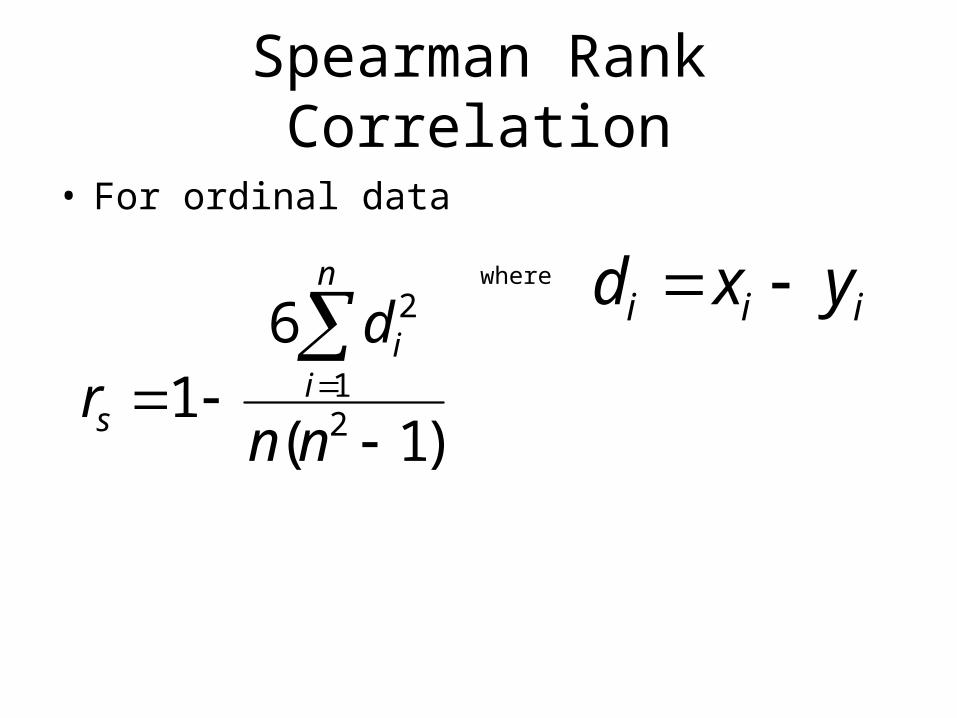
• For ordinal data

)1(

61

21

2

nn

dr

n

ii

s

where

iii yxd

Cross-Correlation

])y(yn[])x(xn[

yxyxnr

2i

2i

*2i

2i

*

iiii*

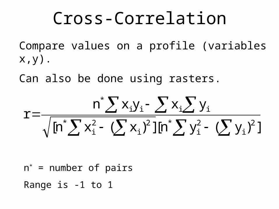
n* = number of pairs

Range is -1 to 1

Compare values on a profile (variables x,y).

Can also be done using rasters.

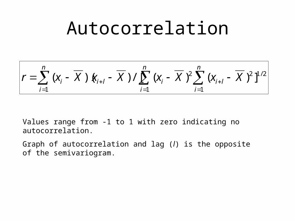
Autocorrelation

2/12

1

2

11

])()(/[))((

n

ili

n

iili

n

ii XxXxXxXxr

Values range from -1 to 1 with zero indicating no autocorrelation.

Graph of autocorrelation and lag (l) is the opposite of the semivariogram.

Other Measures for Spatial Autocorrelation

Moran’s I

Geary’s C

Spatial Autocorrelation

• First law of geography: “everything is related to everything else, but near things are more related than distant things” – Waldo Tobler

• Many geographers would say “I don’t understand spatial autocorrelation” Actually, they don’t understand the mechanics, they do understand the concept.

Spatial Autocorrelation

• Spatial Autocorrelation – correlation of a variable with itself through space.– If there is any systematic pattern in the spatial

distribution of a variable, it is said to be spatially autocorrelated

– If nearby or neighboring areas are more alike, this is positive spatial autocorrelation

– Negative autocorrelation describes patterns in which neighboring areas are unlike

– Random patterns exhibit no spatial autocorrelation

Why spatial autocorrelation is important

• Most statistics are based on the assumption that the values of observations in each sample are independent of one another

• Positive spatial autocorrelation may violate this, if the samples were taken from nearby areas

• Goals of spatial autocorrelation– Measure the strength of spatial autocorrelation in a

map – test the assumption of independence or randomness

Spatial Autocorrelation

• Spatial Autocorrelation is, conceptually as well as empirically, the two-dimensional equivalent of redundancy

• It measures the extent to which the occurrence of an event in an areal unit constrains, or makes more probable, the occurrence of an event in a neighboring areal unit.

Spatial Autocorrelation

• Non-spatial independence suggests many statistical tools and inferences are inappropriate.– Correlation coefficients or ordinary least squares regressions

(OLS) to predict a consequence assumes that the observations have been selected randomly.

– If the observations, however, are spatially clustered in some way, the estimates obtained from the correlation coefficient or OLS estimator will be biased and overly precise.

– They are biased because the areas with higher concentration of events will have a greater impact on the model estimate and they will overestimate precision because, since events tend to be concentrated, there are actually fewer number of independent observations than are being assumed.

Indices of Spatial Autocorrelation (for Areas and/or Points)

• Moran’s I

• Geary’s C

• Ripley’s K

• LISA

• Join Count Analysis

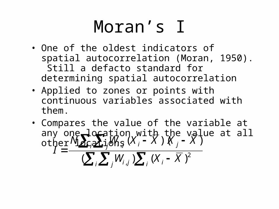
Moran’s I• One of the oldest indicators of spatial

autocorrelation (Moran, 1950). Still a defacto standard for determining spatial autocorrelation

• Applied to zones or points with continuous variables associated with them.

• Compares the value of the variable at any one location with the value at all other locations

i j i iji

i j jiji

XXW

XXXXWNI

2,

,

)()(

))((

Moran’s I

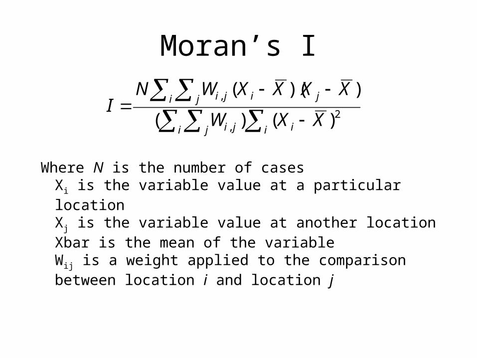
Where N is the number of casesXi is the variable value at a particular locationXj is the variable value at another locationXbar is the mean of the variableWij is a weight applied to the comparison between location i and location j

i j i iji

i j jiji

XXW

XXXXWNI

2,

,

)()(

))((

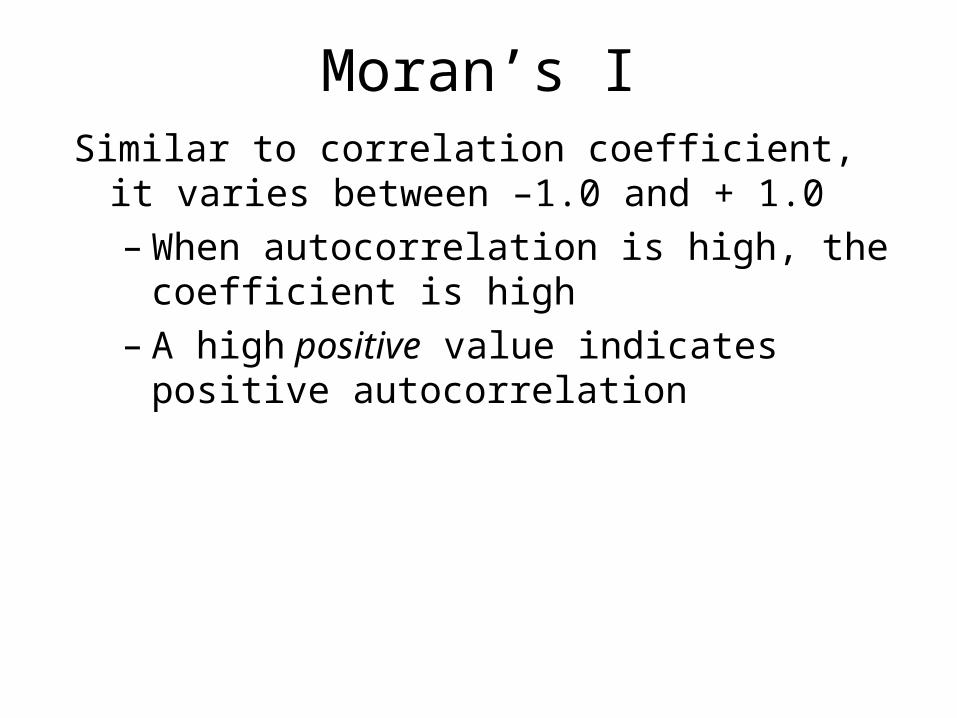
Moran’s ISimilar to correlation coefficient, it varies between

–1.0 and + 1.0– When autocorrelation is high, the coefficient is

high– A high positive value indicates positive

autocorrelation

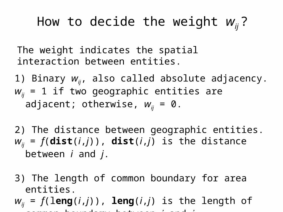
How to decide the weight wij ?

1) Binary wij, also called absolute adjacency. wij = 1 if two geographic entities are adjacent; otherwise, wij =

0.

2) The distance between geographic entities.wij = f(dist(i,j)), dist(i,j) is the distance between i and j.

3) The length of common boundary for area entities.wij = f(leng(i,j)), leng(i,j) is the length of common boundary

between i and j.

The weight indicates the spatial interaction between entities.

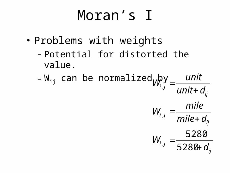
Moran’s I

• Problems with weights– Potential for distorted the value.

– Wij can be normalized by

ijji

ijji

ijji

dW

dmile

mileW

dunit

unitW

5280

5280,

,

,

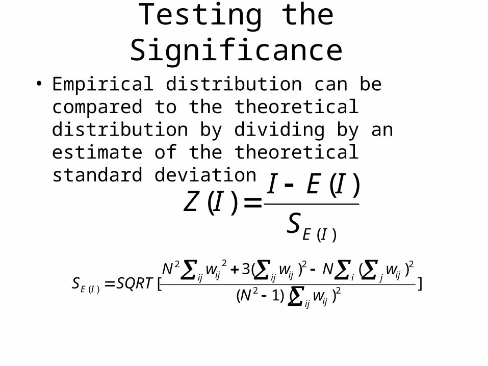
Testing the Significance

• Empirical distribution can be compared to the theoretical distribution by dividing by an estimate of the theoretical standard deviation

)(

)()(

IES

IEIIZ

]))(1(

)()(3[

22

2222

)(

ij ij

ij ij i j ijijij

IE wN

wNwwNSQRTS

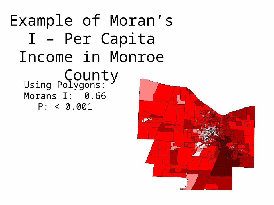
Example of Moran’s I – Per Capita Income in

Monroe County

Using Polygons:Morans I: 0.66

P: < 0.001

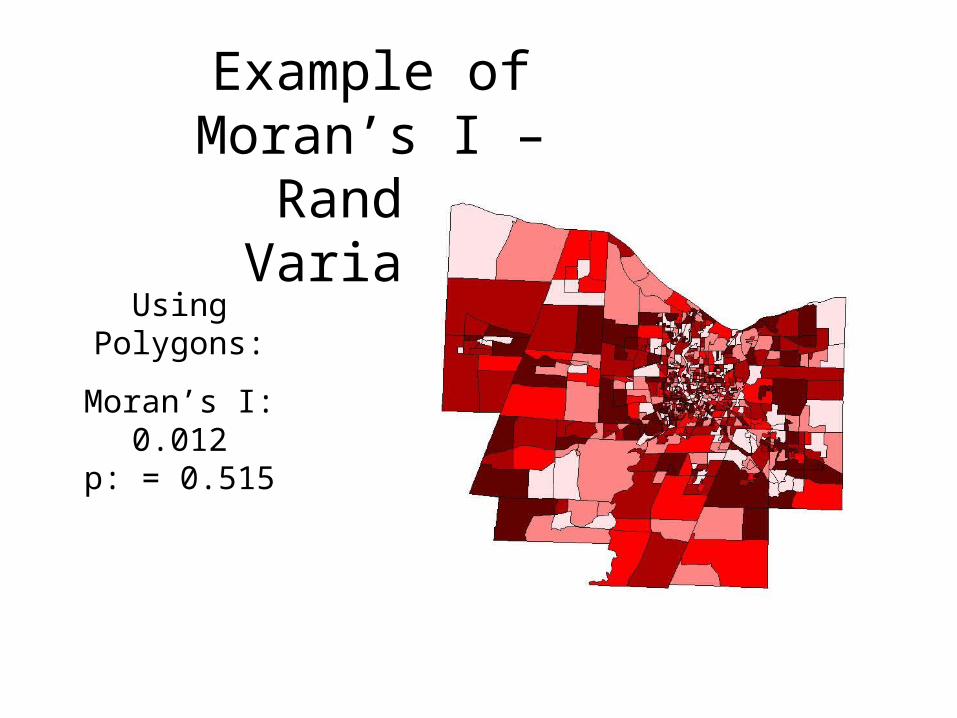
Example of Moran’s I – Random Variable

Using Polygons:

Moran’s I: 0.012p: = 0.515

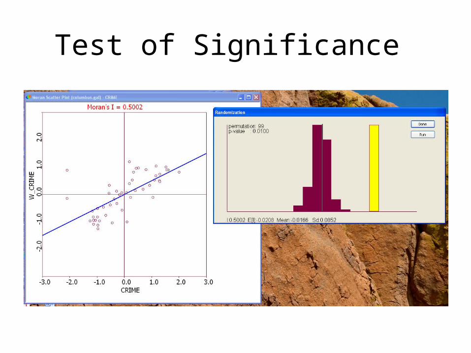
Test of Significance

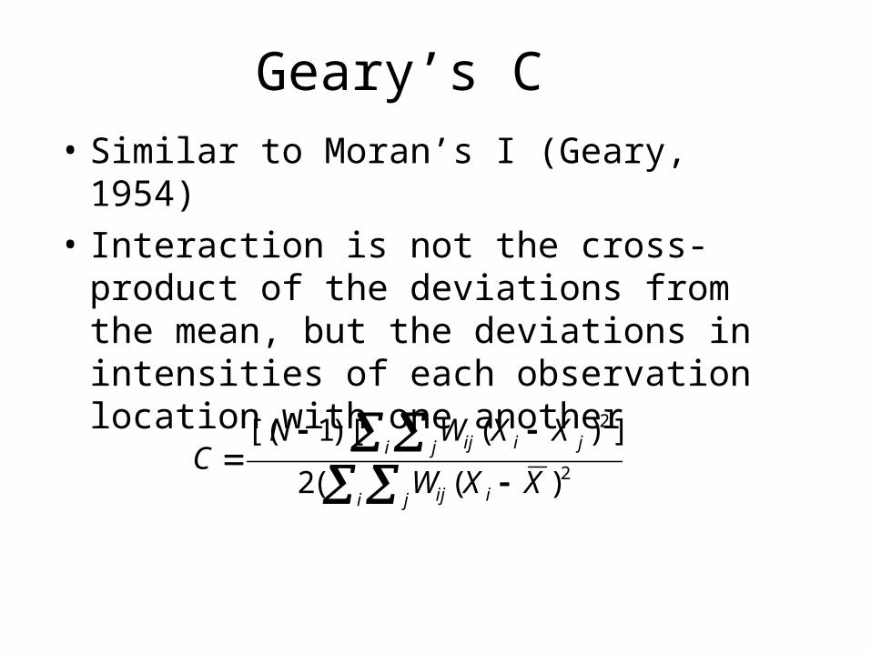
Geary’s C

• Similar to Moran’s I (Geary, 1954)

• Interaction is not the cross-product of the deviations from the mean, but the deviations in intensities of each observation location with one another

i j iij

i j jiij

XXW

XXWNC

2

2

)((2

])()[1[(

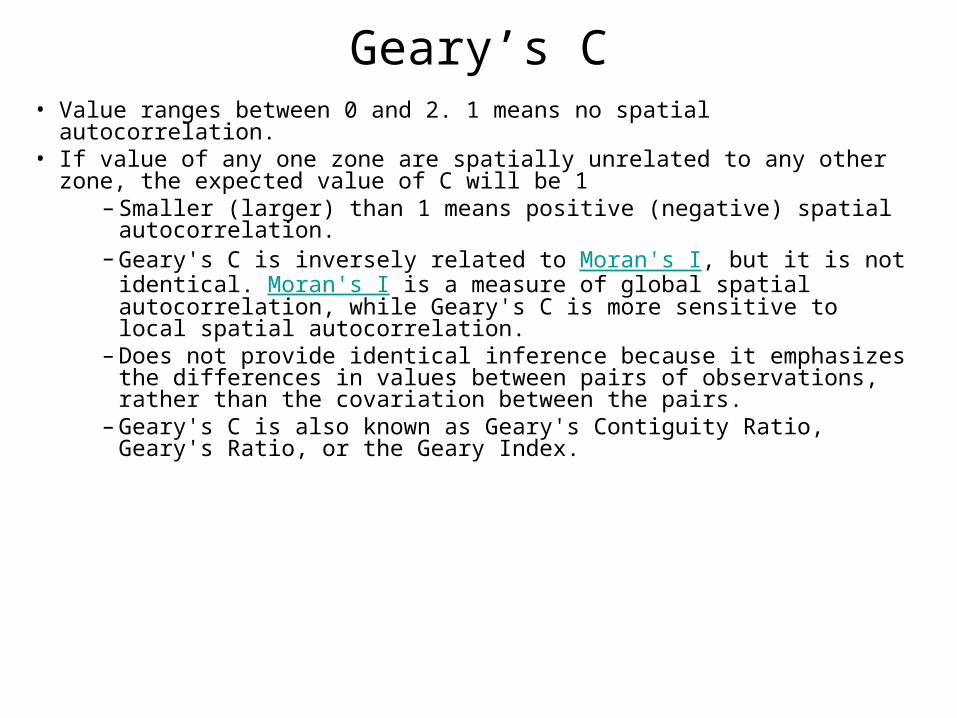
Geary’s C• Value ranges between 0 and 2. 1 means no spatial autocorrelation. • If value of any one zone are spatially unrelated to any other zone, the

expected value of C will be 1 – Smaller (larger) than 1 means positive (negative) spatial

autocorrelation.– Geary's C is inversely related to Moran's I, but it is not identical.

Moran's I is a measure of global spatial autocorrelation, while Geary's C is more sensitive to local spatial autocorrelation.

– Does not provide identical inference because it emphasizes the differences in values between pairs of observations, rather than the covariation between the pairs.

– Geary's C is also known as Geary's Contiguity Ratio, Geary's Ratio, or the Geary Index.

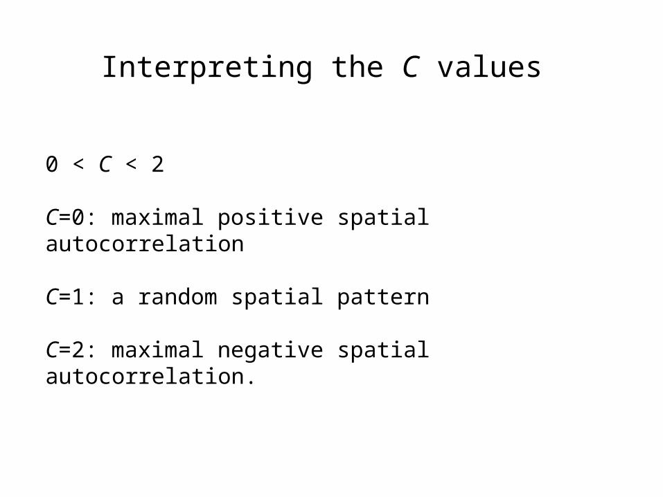
Interpreting the C values

0 < C < 2

C=0: maximal positive spatial autocorrelation

C=1: a random spatial pattern

C=2: maximal negative spatial autocorrelation.

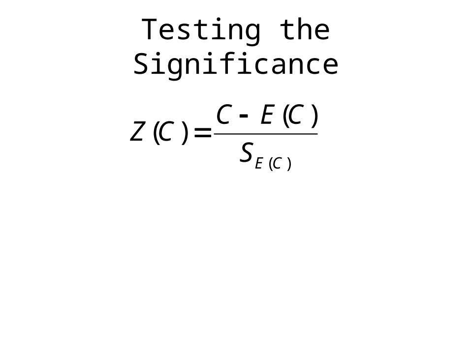
Testing the Significance

)(

)()(

CES

CECCZ

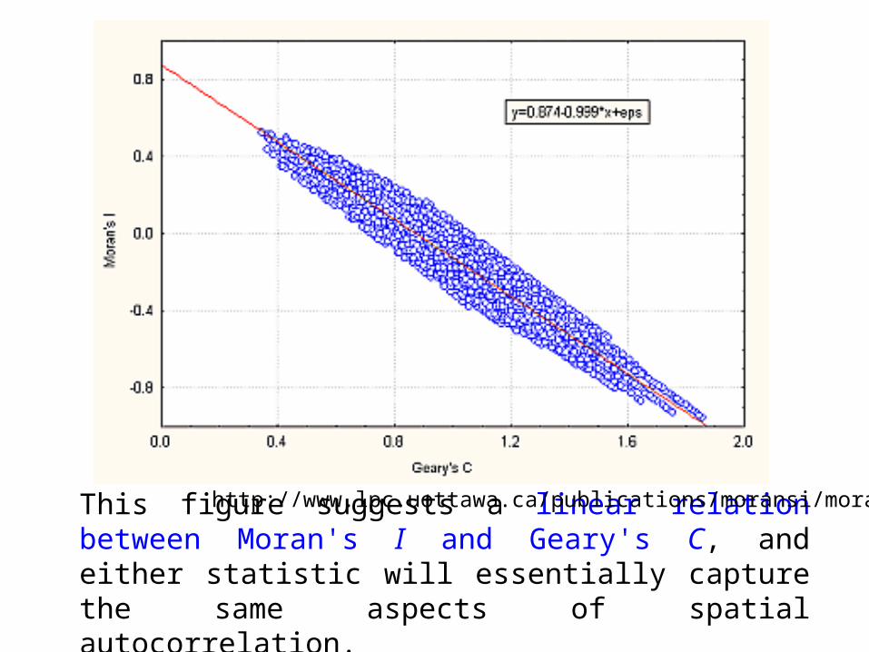
This figure suggests a linear relation between Moran's I and Geary's C, and either statistic will essentially capture the same aspects of spatial autocorrelation.

http://www.lpc.uottawa.ca/publications/moransi/moran.htm