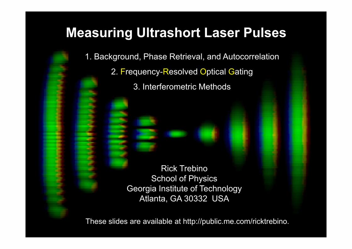
Measuring Ultrashort Laser Pulses

Rick Trebino

School of Physics

Georgia Institute of Technology

Atlanta, GA 30332 USA

1. Background, Phase Retrieval, and Autocorrelation

2. Frequency-Resolved Optical Gating

3. Interferometric Methods

These slides are available at http://public.me.com/ricktrebino.

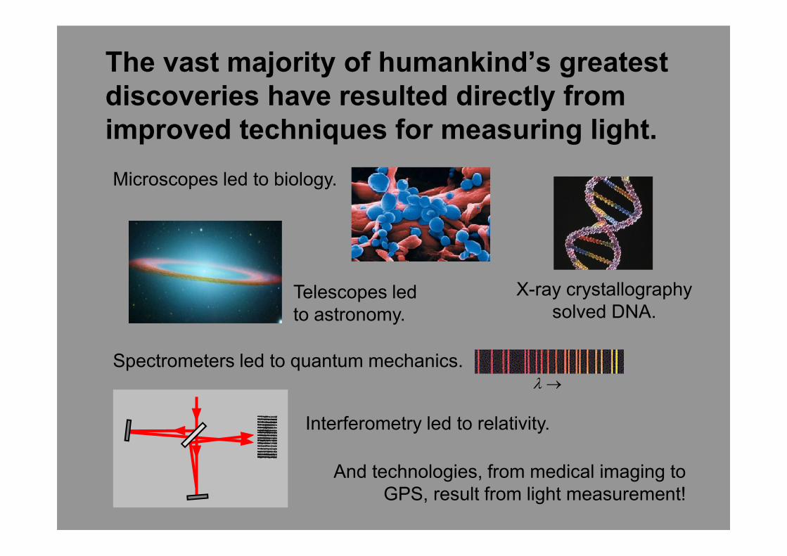
The vast majority of humankind’s greatest

discoveries have resulted directly from

improved techniques for measuring light.

λ →Spectrometers led to quantum mechanics.

Interferometry led to relativity.

Microscopes led to biology.

Telescopes led

to astronomy.

X-ray crystallography

solved DNA.

And technologies, from medical imaging to

GPS, result from light measurement!

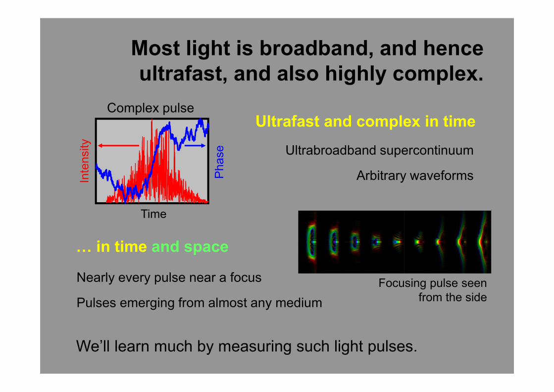
Most light is broadband, and hence

ultrafast, and also highly complex.

Ultrabroadband supercontinuum

Arbitrary waveforms

Ultrafast and complex in time

" in time and space

Nearly every pulse near a focus

Pulses emerging from almost any medium

We’ll learn much by measuring such light pulses.

Focusing pulse seen

from the side

Complex pulse

Time

Inte

nsity

Phase

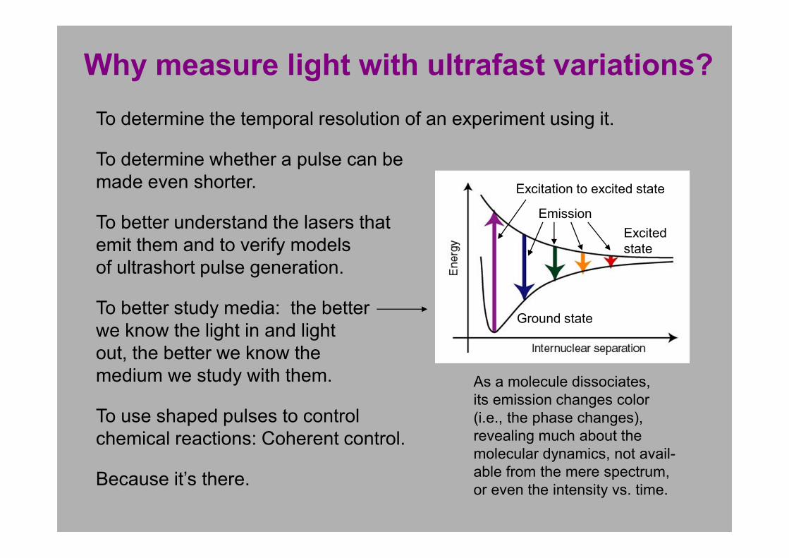
To determine the temporal resolution of an experiment using it.

To determine whether a pulse can be

made even shorter.

To better understand the lasers that

emit them and to verify models

of ultrashort pulse generation.

To better study media: the better

we know the light in and light

out, the better we know the

medium we study with them.

To use shaped pulses to control

chemical reactions: Coherent control.

Because it’s there.

Why measure light with ultrafast variations?

As a molecule dissociates,

its emission changes color

(i.e., the phase changes),

revealing much about the

molecular dynamics, not avail-

able from the mere spectrum,

or even the intensity vs. time.

Excitation to excited state

Emission

Ground state

Excited

state

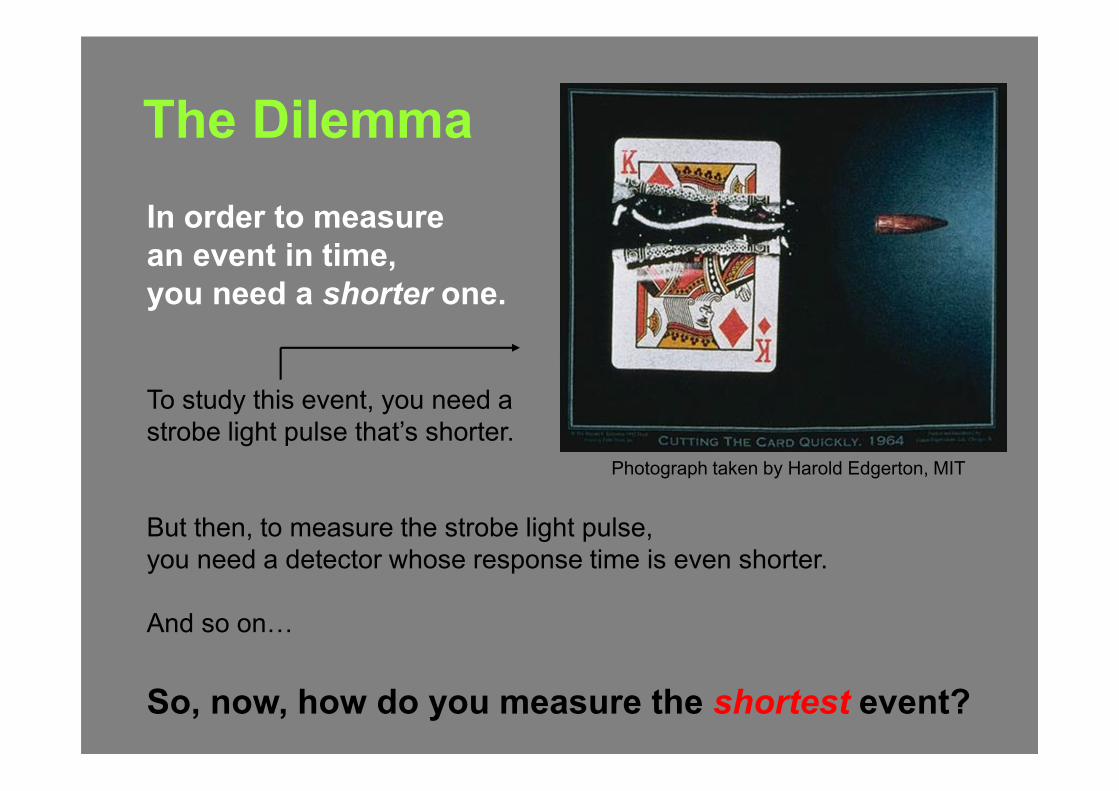
In order to measure

an event in time,

you need a shorter one.

To study this event, you need a

strobe light pulse that’s shorter.

But then, to measure the strobe light pulse,

you need a detector whose response time is even shorter.

And so on9

So, now, how do you measure the shortest event?

Photograph taken by Harold Edgerton, MIT

The Dilemma

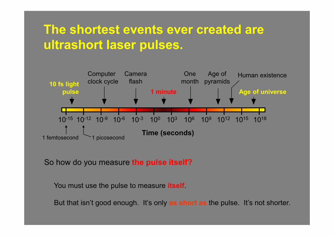
The shortest events ever created are

ultrashort laser pulses.

So how do you measure the pulse itself?

You must use the pulse to measure itself.

But that isn’t good enough. It’s only as short as the pulse. It’s not shorter.

1 minute

10 fs light

pulse Age of universe

Time (seconds)

Computer

clock cycle

Camera

flash

Age of

pyramids

One

monthHuman existence

10-15 10-12 10-9 10-6 10-3 100 103 106 109 1012 1015 1018

1 femtosecond 1 picosecond

Intensity Autocorrelation1D Phase Retrieval

Single-shot autocorrelation

The Autocorrelation and SpectrumAmbiguities

Third-order Autocorrelation

Interferometric Autocorrelation

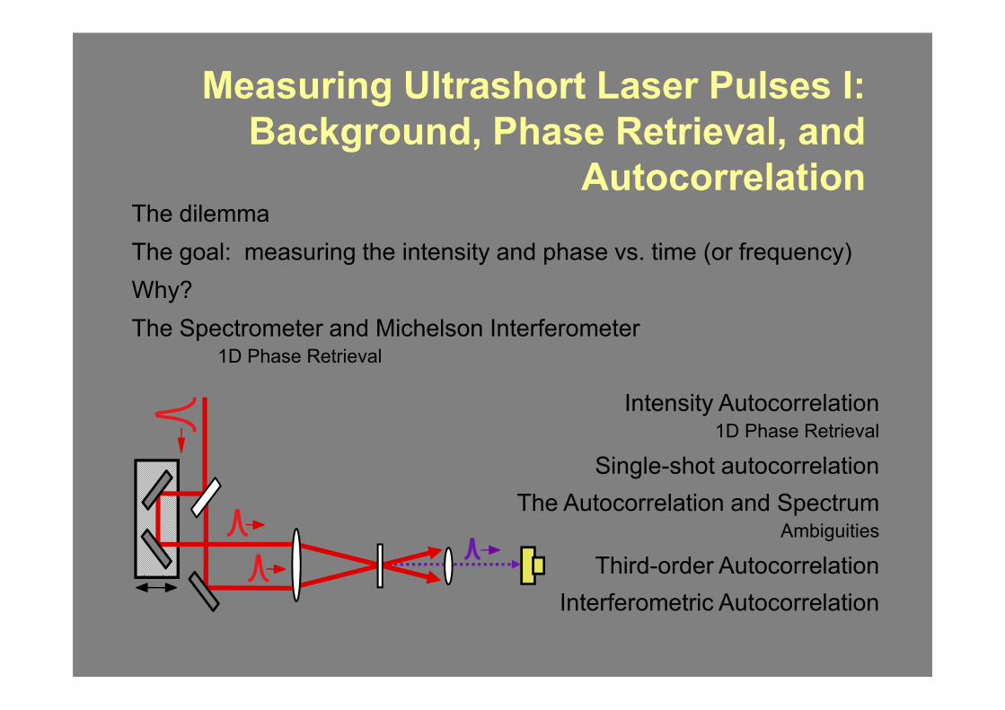
Measuring Ultrashort Laser Pulses I:

Background, Phase Retrieval, and

AutocorrelationThe dilemma

The goal: measuring the intensity and phase vs. time (or frequency)

Why?

The Spectrometer and Michelson Interferometer1D Phase Retrieval

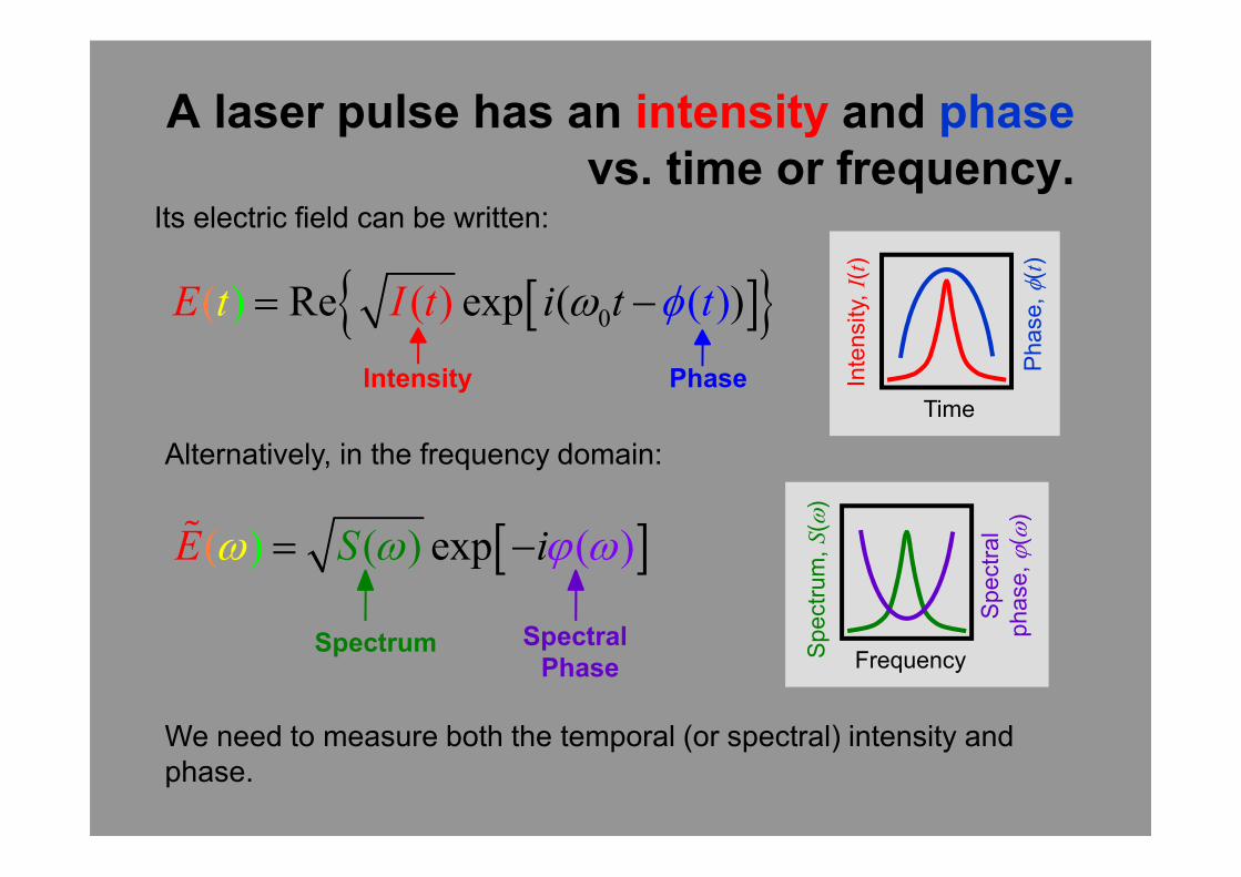
Its electric field can be written:

Intensity Phase

[ ]{ }0Re exp ( (( ))( )) iE It tt tω φ= −

Alternatively, in the frequency domain:

Spectral

PhaseSpectrum

[ ]( ) exp ))( (SE iω ωω ϕ= −%

We need to measure both the temporal (or spectral) intensity and

phase.

A laser pulse has an intensity and phase

vs. time or frequency.

Sp

ectr

al

ph

ase

, ϕ(

ω)

FrequencySp

ectr

um

, S(ω

)

Ph

ase

, φ(t)

Time

Inte

nsity,

I(t

)

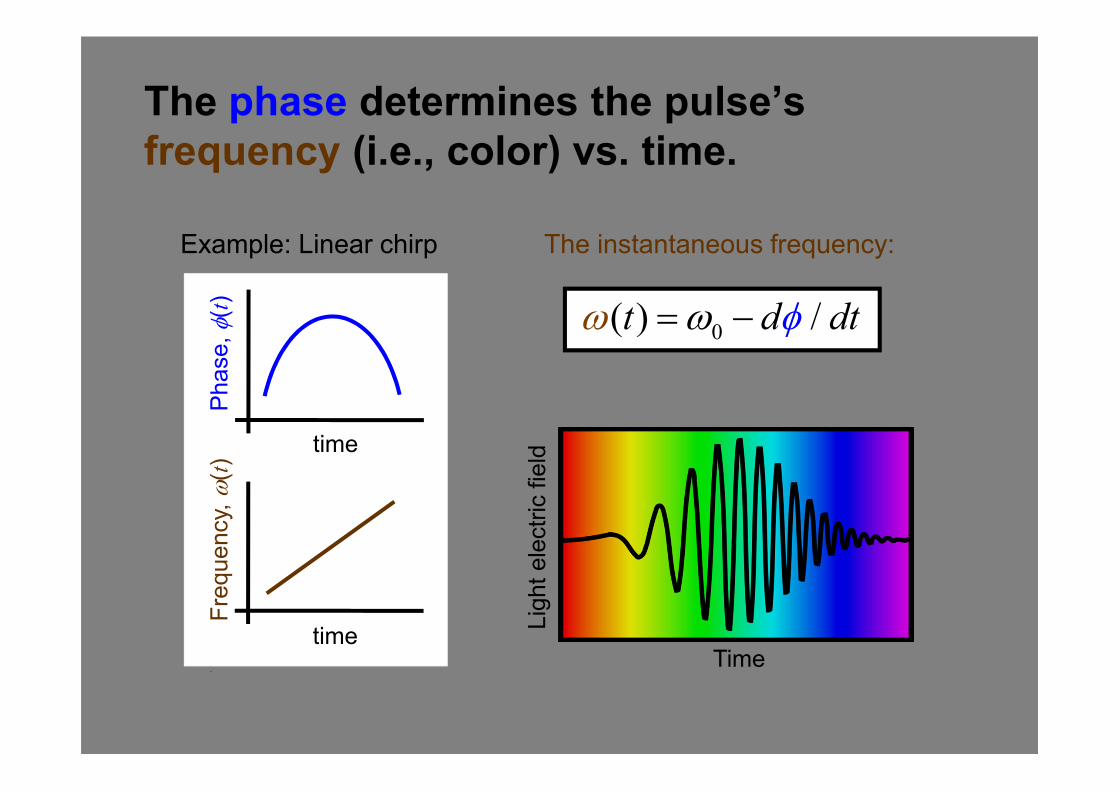
The instantaneous frequency:Example: Linear chirp P

hase, φ(t)

time

time

Fre

quency,

ω(t

)

time

The phase determines the pulse’s

frequency (i.e., color) vs. time.

0( ) /t d dtω φω= −

Time

Lig

ht

ele

ctr

ic f

ield

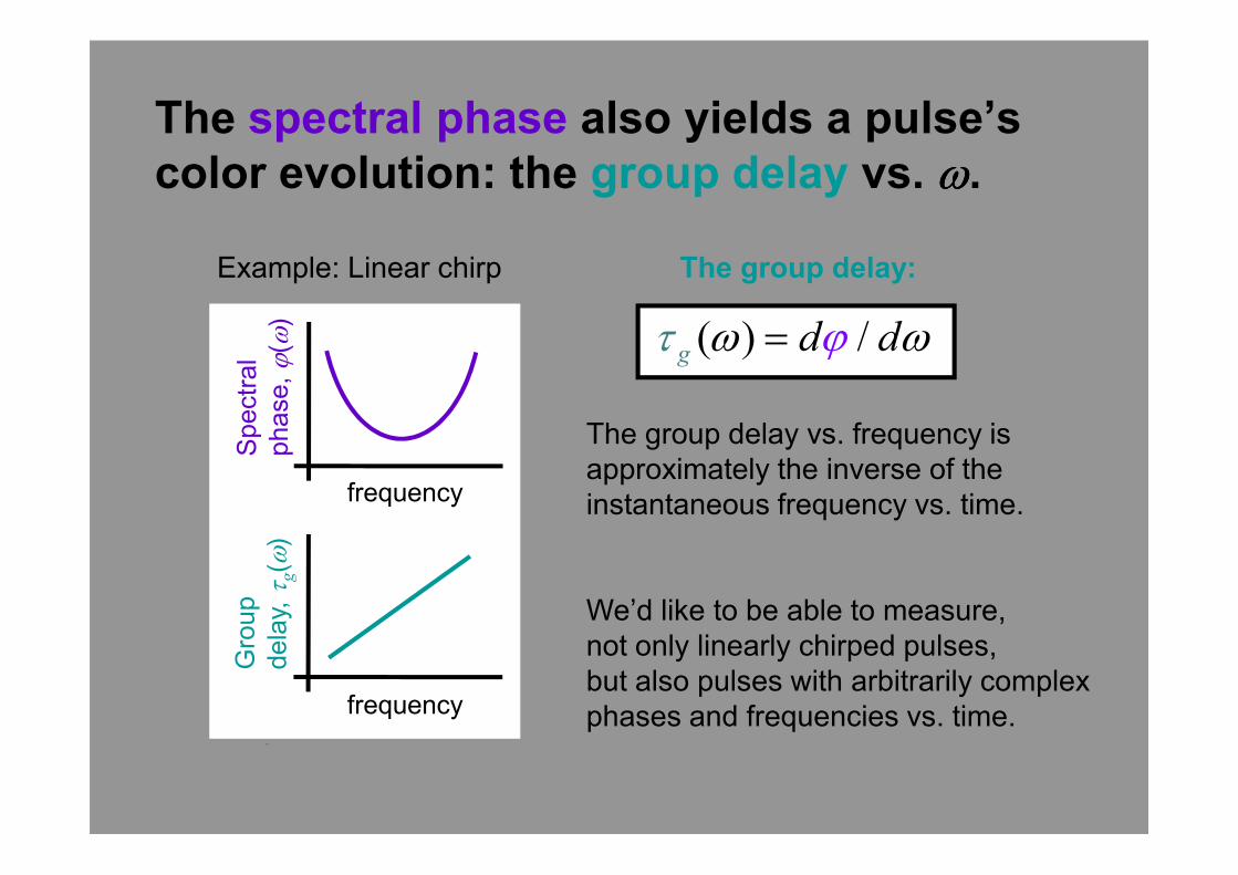
The group delay:Example: Linear chirp S

pectr

al

phase, ϕ(

ω)

frequency

frequency

Gro

up

dela

y, τg( ω

)

time

The group delay vs. frequency is

approximately the inverse of the

instantaneous frequency vs. time.

The spectral phase also yields a pulse’s

color evolution: the group delay vs. ωωωω.

( ) /g d dτ ϕω ω=

We’d like to be able to measure,

not only linearly chirped pulses,

but also pulses with arbitrarily complex

phases and frequencies vs. time.

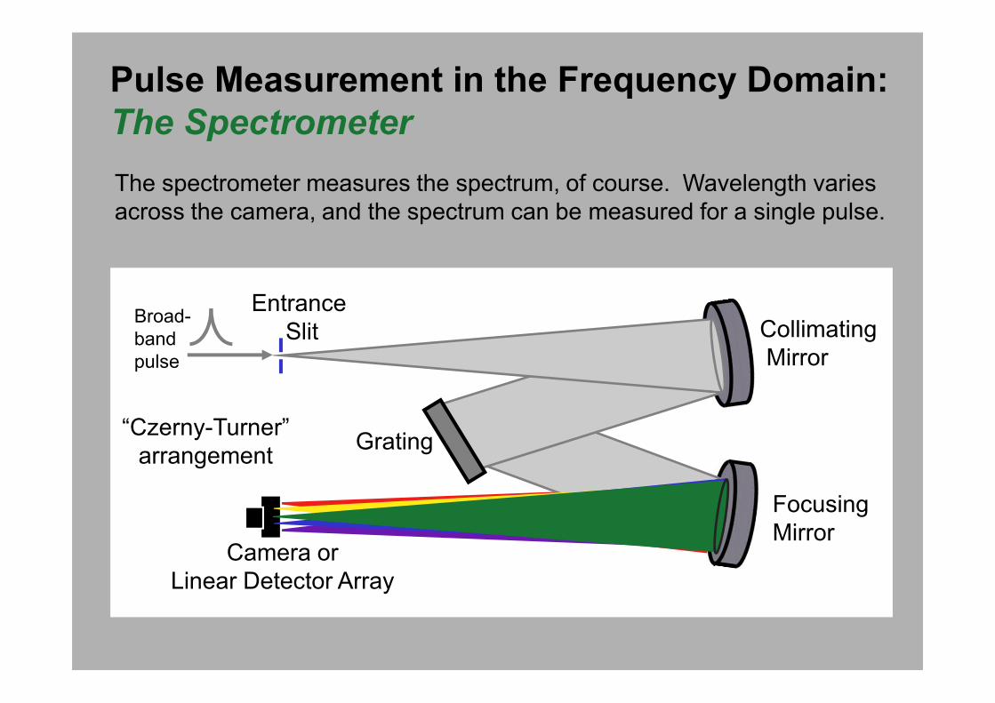
The spectrometer measures the spectrum, of course. Wavelength varies

across the camera, and the spectrum can be measured for a single pulse.

Pulse Measurement in the Frequency Domain:

The Spectrometer

Collimating

Mirror

“Czerny-Turner”

arrangement

Entrance

Slit

Camera or

Linear Detector Array

Focusing

Mirror

Grating

Broad-

band

pulse

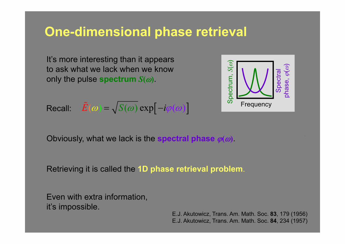
One-dimensional phase retrieval

E.J. Akutowicz, Trans. Am. Math. Soc. 83, 179 (1956)

E.J. Akutowicz, Trans. Am. Math. Soc. 84, 234 (1957)

Retrieving it is called the 1D phase retrieval problem.

It’s more interesting than it appears

to ask what we lack when we know

only the pulse spectrum S(ωωωω).

Obviously, what we lack is the spectral phase ϕϕϕϕ(ωωωω).

Even with extra information,

it’s impossible.

Recall:

time

Sp

ectr

al

ph

ase

, ϕ(

ω)

FrequencySp

ectr

um

, S(ω

)

[ ]( ) exp ))( (SE iω ωω ϕ= −%

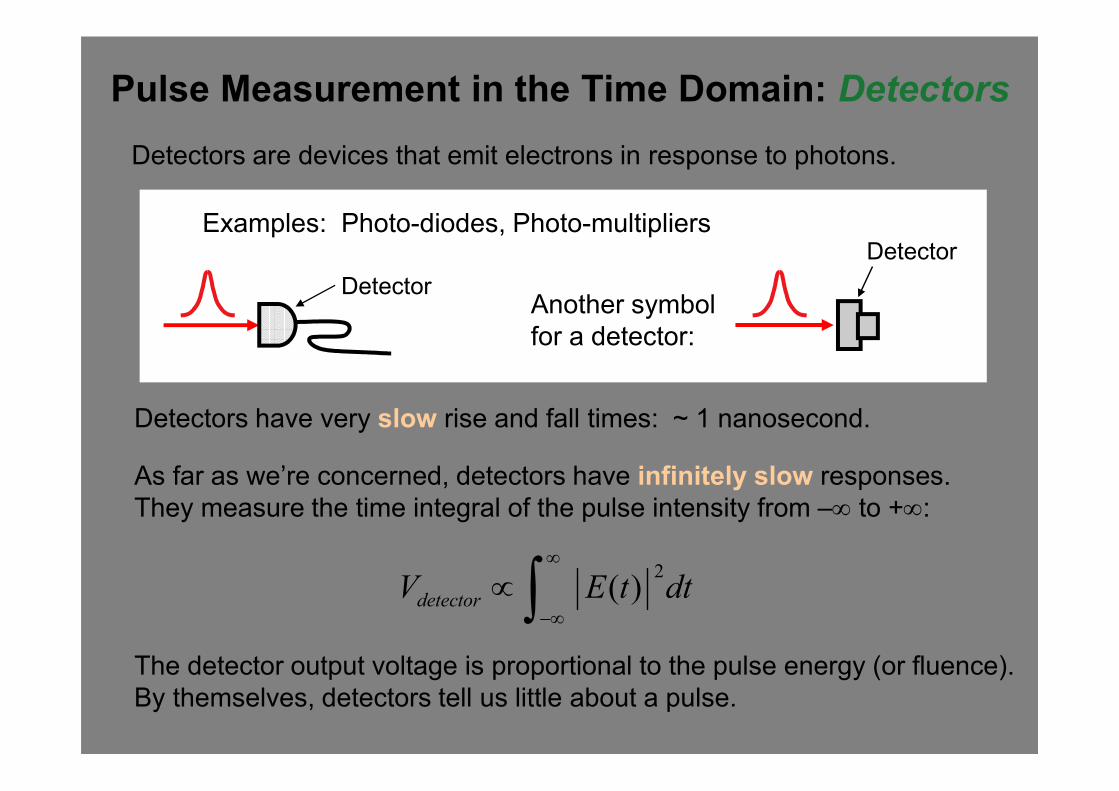
Pulse Measurement in the Time Domain: Detectors

Examples: Photo-diodes, Photo-multipliers

Detectors are devices that emit electrons in response to photons.

Detectors have very slow rise and fall times: ~ 1 nanosecond.

As far as we’re concerned, detectors have infinitely slow responses.

They measure the time integral of the pulse intensity from –∞ to +∞:

The detector output voltage is proportional to the pulse energy (or fluence).

By themselves, detectors tell us little about a pulse.

2( )detectorV E t dt

∞

−∞∝ ∫

Another symbol

for a detector:

Detector

Detector

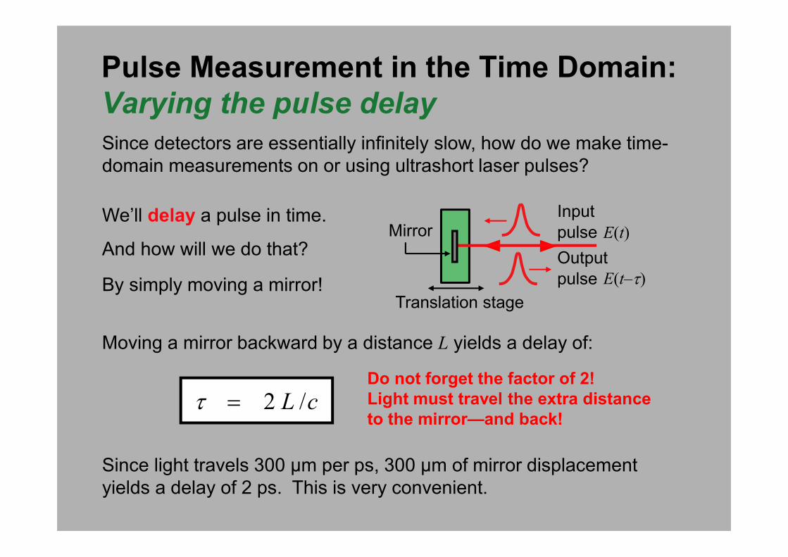
Translation stage

Pulse Measurement in the Time Domain:

Varying the pulse delay

Since detectors are essentially infinitely slow, how do we make time-

domain measurements on or using ultrashort laser pulses?

We’ll delay a pulse in time.

And how will we do that?

By simply moving a mirror!

Since light travels 300 µm per ps, 300 µm of mirror displacement

yields a delay of 2 ps. This is very convenient.

Moving a mirror backward by a distance L yields a delay of:

τ = 2 L /cDo not forget the factor of 2!

Light must travel the extra distance

to the mirror—and back!

Input

pulse E(t)

E(t–τ)

Mirror

Output

pulse

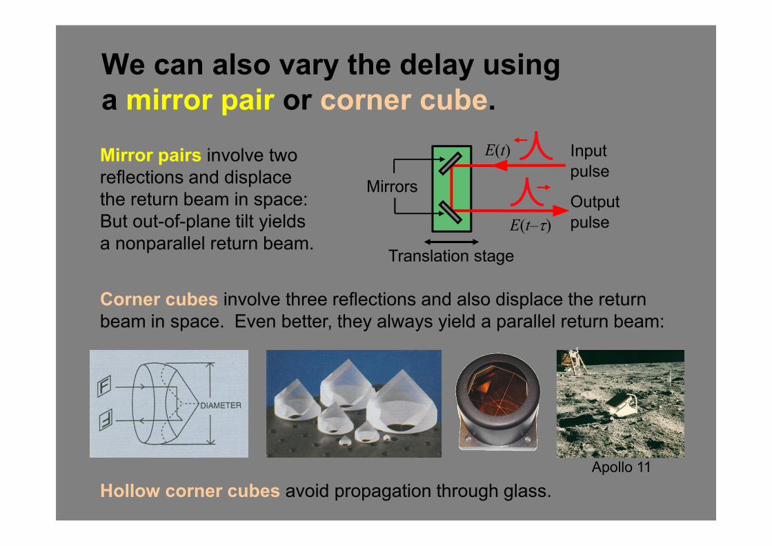
We can also vary the delay using

a mirror pair or corner cube.

Mirror pairs involve two

reflections and displace

the return beam in space:

But out-of-plane tilt yields

a nonparallel return beam.

Corner cubes involve three reflections and also displace the return

beam in space. Even better, they always yield a parallel return beam:

Hollow corner cubes avoid propagation through glass.

Translation stage

Input

pulse

E(t)

E(t–τ)

MirrorsOutput

pulse

Apollo 11

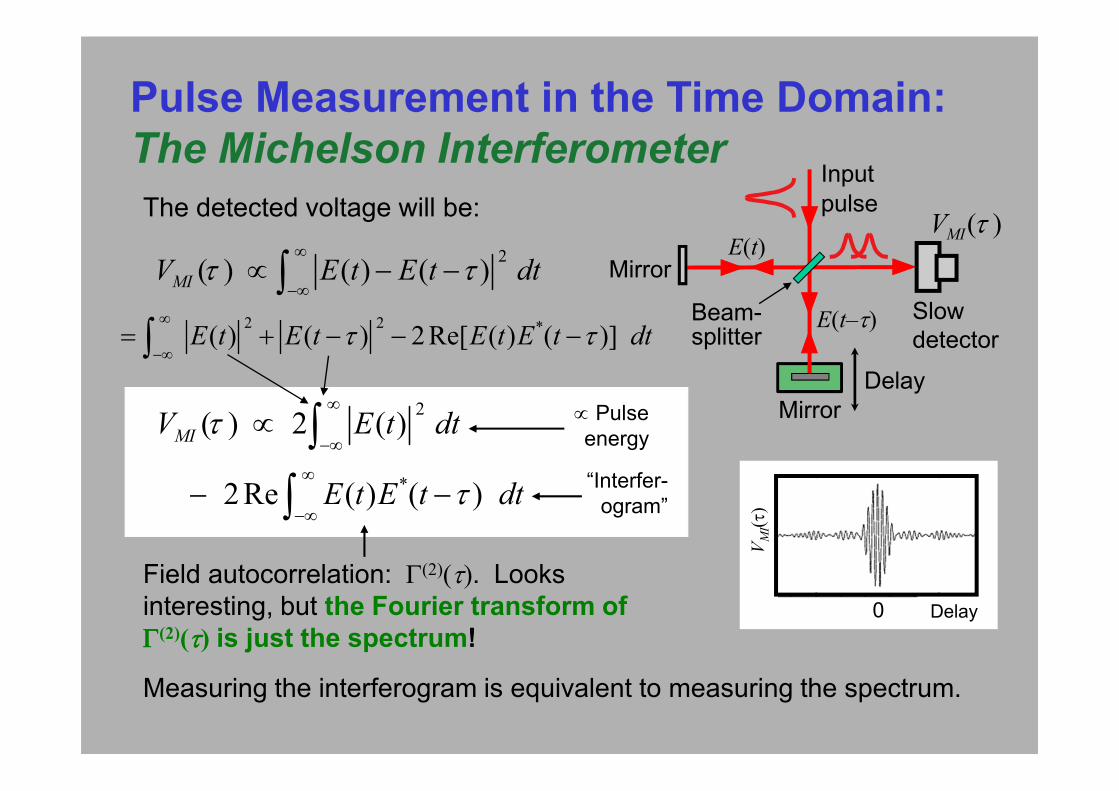
Measuring the interferogram is equivalent to measuring the spectrum.

Pulse Measurement in the Time Domain:

The Michelson Interferometer

2 2 *( ) ( ) 2Re[ ( ) ( )]E t E t E t E t dtτ τ∞

−∞= + − − −∫

2( ) ( ) ( )MIV E t E t dtτ τ

∞

−∞∝ − −∫

2

*

( ) 2 ( )

2Re ( ) ( )

MIV E t dt

E t E t dt

τ

τ

∞

−∞

∞

−∞

∝

− −

∫

∫

∝ Pulse

energy

Field autocorrelation: Γ(2)(τ). Looks

interesting, but the Fourier transform of

ΓΓΓΓ(2)(ττττ) is just the spectrum!

Beam-splitter

Input

pulse

Delay

Slow

detector

Mirror

Mirror

E(t)

E(t–τ)

VMI(τ )

“Interfer-

ogram”

⇒VMI(τ)

0 Delay

The detected voltage will be:

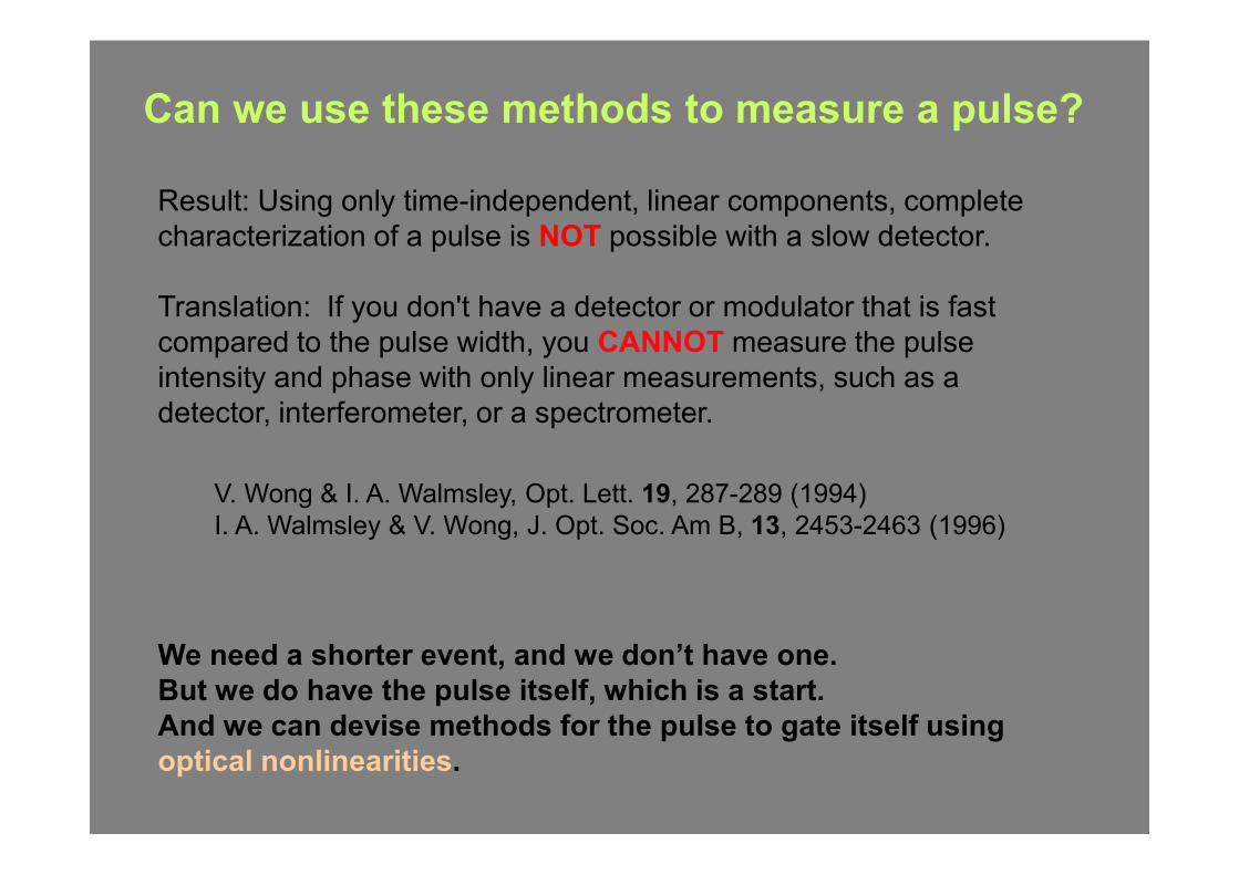
Can we use these methods to measure a pulse?

V. Wong & I. A. Walmsley, Opt. Lett. 19, 287-289 (1994)

I. A. Walmsley & V. Wong, J. Opt. Soc. Am B, 13, 2453-2463 (1996)

Result: Using only time-independent, linear components, complete

characterization of a pulse is NOT possible with a slow detector.

Translation: If you don't have a detector or modulator that is fast

compared to the pulse width, you CANNOT measure the pulse

intensity and phase with only linear measurements, such as a

detector, interferometer, or a spectrometer.

We need a shorter event, and we don’t have one.

But we do have the pulse itself, which is a start.

And we can devise methods for the pulse to gate itself using

optical nonlinearities.

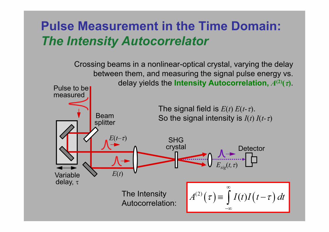
Pulse Measurement in the Time Domain:

The Intensity Autocorrelator

SHG

crystal

The Intensity

Autocorrelation:( ) ( )(2) ( )A I t I t dtτ τ

∞

−∞

≡ −∫

SHGcrystal

Pulse to be measured

Variable delay, τ

Detector

Beamsplitter

E(t)

E(t–τ)

Esig(t,τ)

The signal field is E(t) E(t-τ).So the signal intensity is I(t) I(t-τ)

Crossing beams in a nonlinear-optical crystal, varying the delay

between them, and measuring the signal pulse energy vs.

delay yields the Intensity Autocorrelation, A(2)(ττττ).

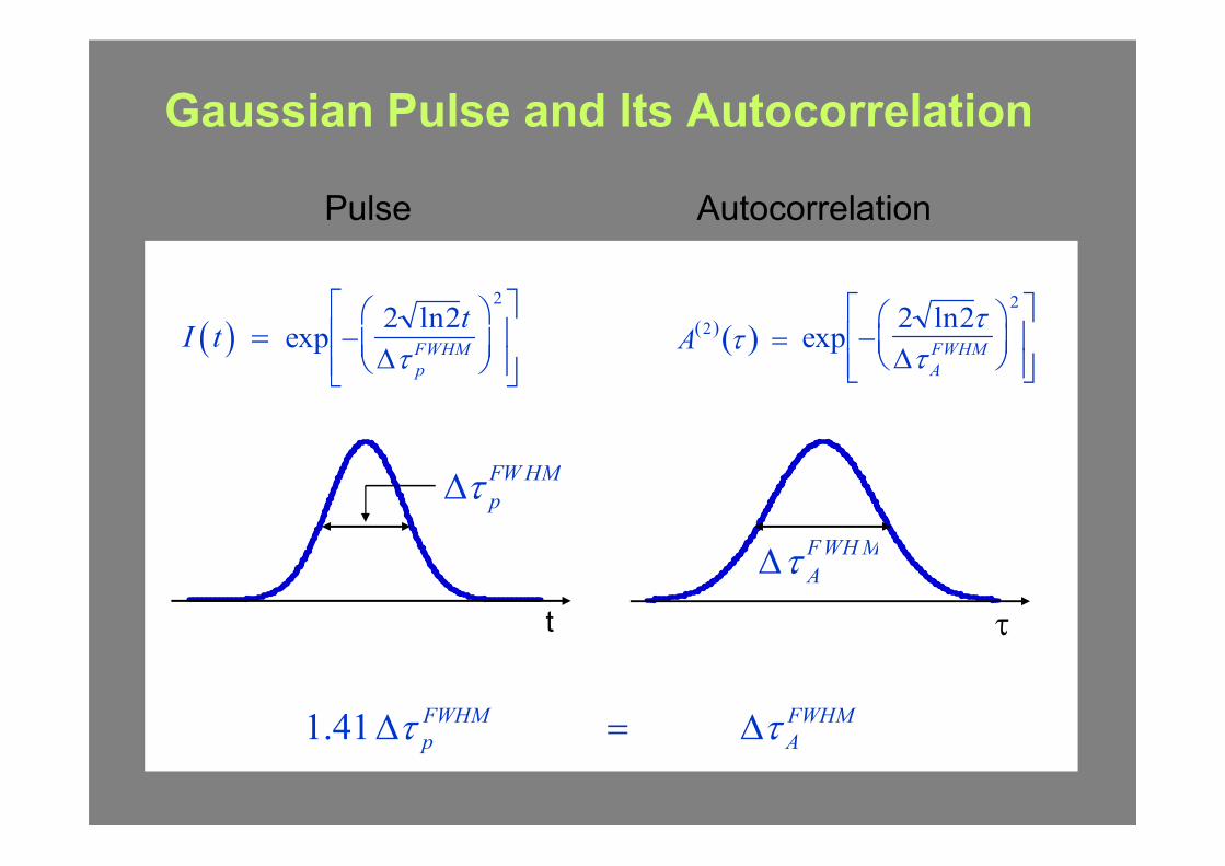
Gaussian Pulse and Its Autocorrelation

Pulse Autocorrelation

t τ

exp −2 ln2t

∆τ pFWHM

2

exp −2 ln2τ∆τA

FWHM

2

( )I t =

1.41 FWHM FWHM

p Aτ τ∆ = ∆

A2( ) τ( ) =

∆τ pFWHM

∆τ AFWHM

Pulse Autocorrelation

t τ

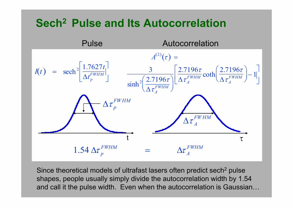
Sech2 Pulse and Its Autocorrelation

sech2 1.7627t

∆t pFWHM

3

sinh2 2.7196τ

∆τAFWHM

2.7196τ∆τA

FWHM coth2.7196τ∆τA

FWHM

−1

I t( ) =

1.54 FWHM FWHM

p Aτ τ∆ = ∆

A2( ) τ( ) =

∆τ pFWHM

∆τ AFWHM

Since theoretical models of ultrafast lasers often predict sech2 pulse

shapes, people usually simply divide the autocorrelation width by 1.54

and call it the pulse width. Even when the autocorrelation is Gaussian9

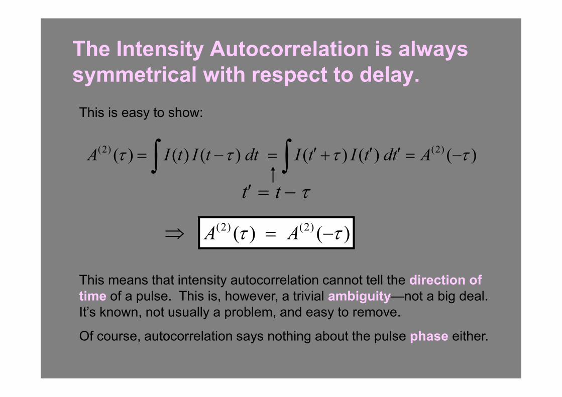
The Intensity Autocorrelation is always

symmetrical with respect to delay.

(2) (2)( ) ( )A Aτ τ= −

(2) (2)( ) ( ) ( ) ( ) ( ) ( )A I t I t dt I t I t dt Aτ τ τ τ′ ′ ′= − = + = −∫ ∫′ t = t − τ

This is easy to show:

⇒

This means that intensity autocorrelation cannot tell the direction of

time of a pulse. This is, however, a trivial ambiguity—not a big deal.

It’s known, not usually a problem, and easy to remove.

Of course, autocorrelation says nothing about the pulse phase either.

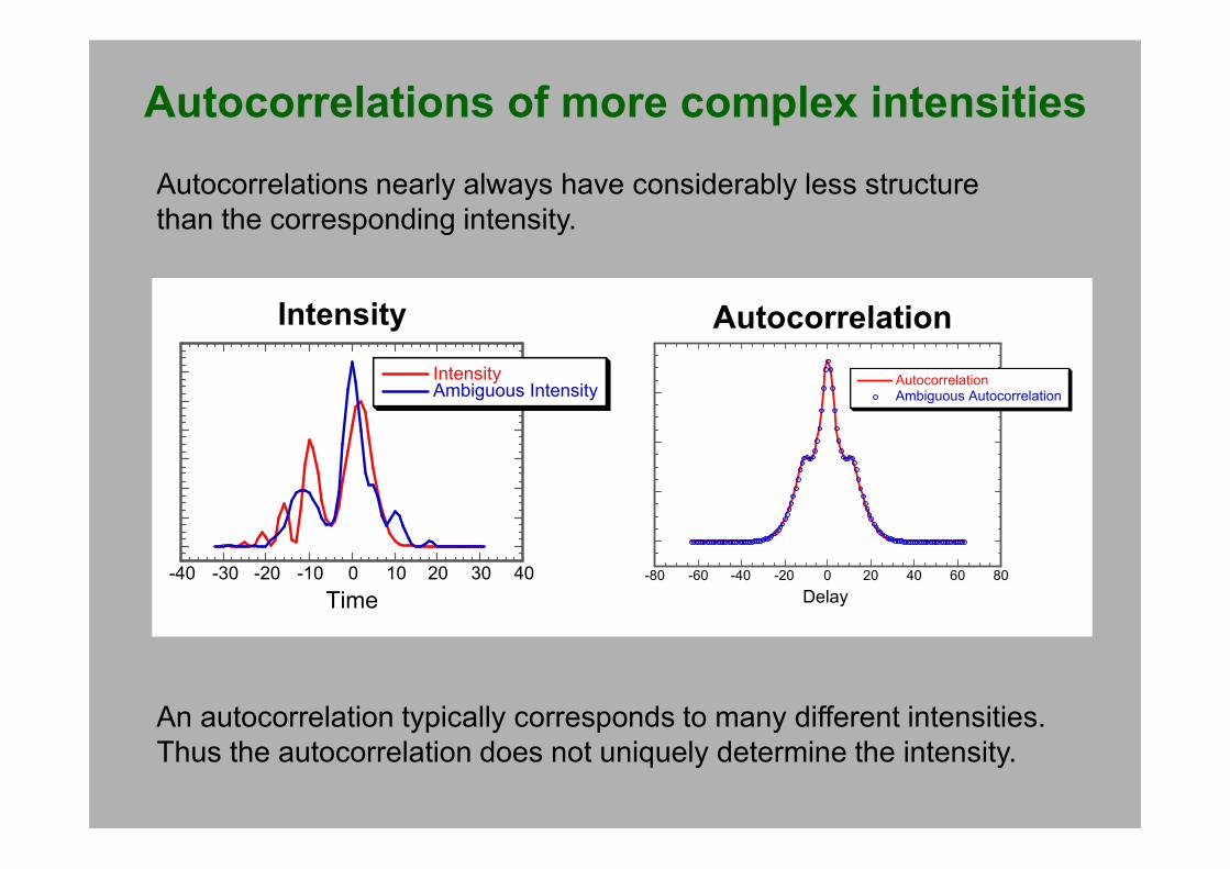
Autocorrelations of more complex intensities

-80 -60 -40 -20 0 20 40 60 80

Autocorrelation

AutocorrelationAmbiguous Autocorrelation

Delay

-40 -30 -20 -10 0 10 20 30 40

Intensity

IntensityAmbiguous Intensity

Time

Autocorrelations nearly always have considerably less structure

than the corresponding intensity.

An autocorrelation typically corresponds to many different intensities.

Thus the autocorrelation does not uniquely determine the intensity.

Autocorrelation

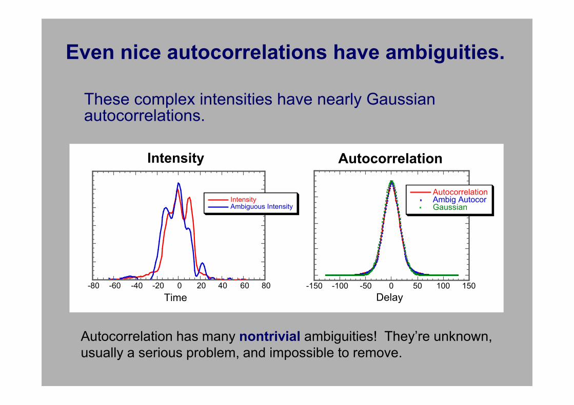
Even nice autocorrelations have ambiguities.

These complex intensities have nearly Gaussian autocorrelations.

-80 -60 -40 -20 0 20 40 60 80

IntensityAmbiguous Intensity

Time

Intensity

-150 -100 -50 0 50 100 150

Autocorrelation

AutocorrelationAmbig AutocorGaussian

Delay

Autocorrelation has many nontrivial ambiguities! They’re unknown,

usually a serious problem, and impossible to remove.

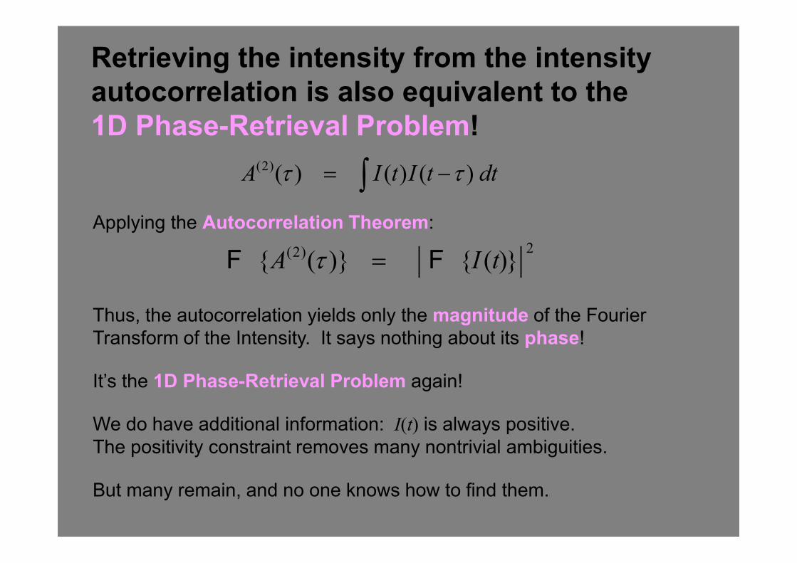
Retrieving the intensity from the intensity

autocorrelation is also equivalent to the

1D Phase-Retrieval Problem!

Applying the Autocorrelation Theorem:

2(2){ ( )} { ( )}A I tτ =F F

Thus, the autocorrelation yields only the magnitude of the Fourier

Transform of the Intensity. It says nothing about its phase!

It’s the 1D Phase-Retrieval Problem again!

We do have additional information: I(t) is always positive.

The positivity constraint removes many nontrivial ambiguities.

But many remain, and no one knows how to find them.

(2)( ) ( ) ( )A I t I t dtτ τ= −∫

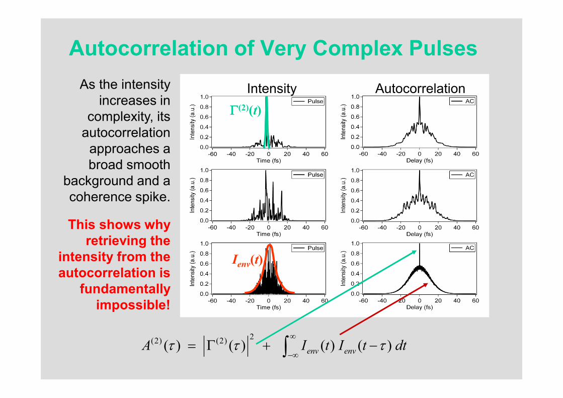
Autocorrelation of Very Complex Pulses

x intens ities with G aussian s low ly v arying

Intensity AutocorrelationAs the intensity

increases in

complexity, its

autocorrelation

approaches a

broad smooth

background and a

coherence spike.

2(2) (2)( ) ( ) ( ) ( )env envA I t I t dtτ τ τ

∞

−∞= Γ + −∫

Ienv(t)

ΓΓΓΓ(2)(t)

This shows why

retrieving the

intensity from the

autocorrelation is

fundamentally

impossible!

x

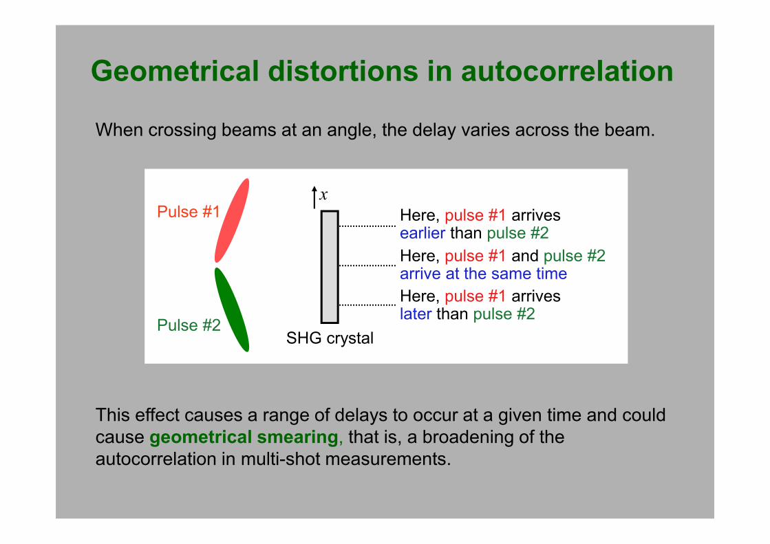
Geometrical distortions in autocorrelation

This effect causes a range of delays to occur at a given time and could

cause geometrical smearing, that is, a broadening of the

autocorrelation in multi-shot measurements.

When crossing beams at an angle, the delay varies across the beam.

Pulse #1

Pulse #2

Here, pulse #1 arrivesearlier than pulse #2

Here, pulse #1 and pulse #2arrive at the same time

Here, pulse #1 arriveslater than pulse #2

SHG crystal

xx

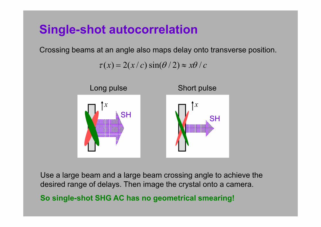
Single-shot autocorrelation

Use a large beam and a large beam crossing angle to achieve the

desired range of delays. Then image the crystal onto a camera.

So single-shot SHG AC has no geometrical smearing!

Crossing beams at an angle also maps delay onto transverse position.

( ) 2( / ) sin( / 2) /x x c x cτ θ θ= ≈

Long pulse Short pulse

SHSH

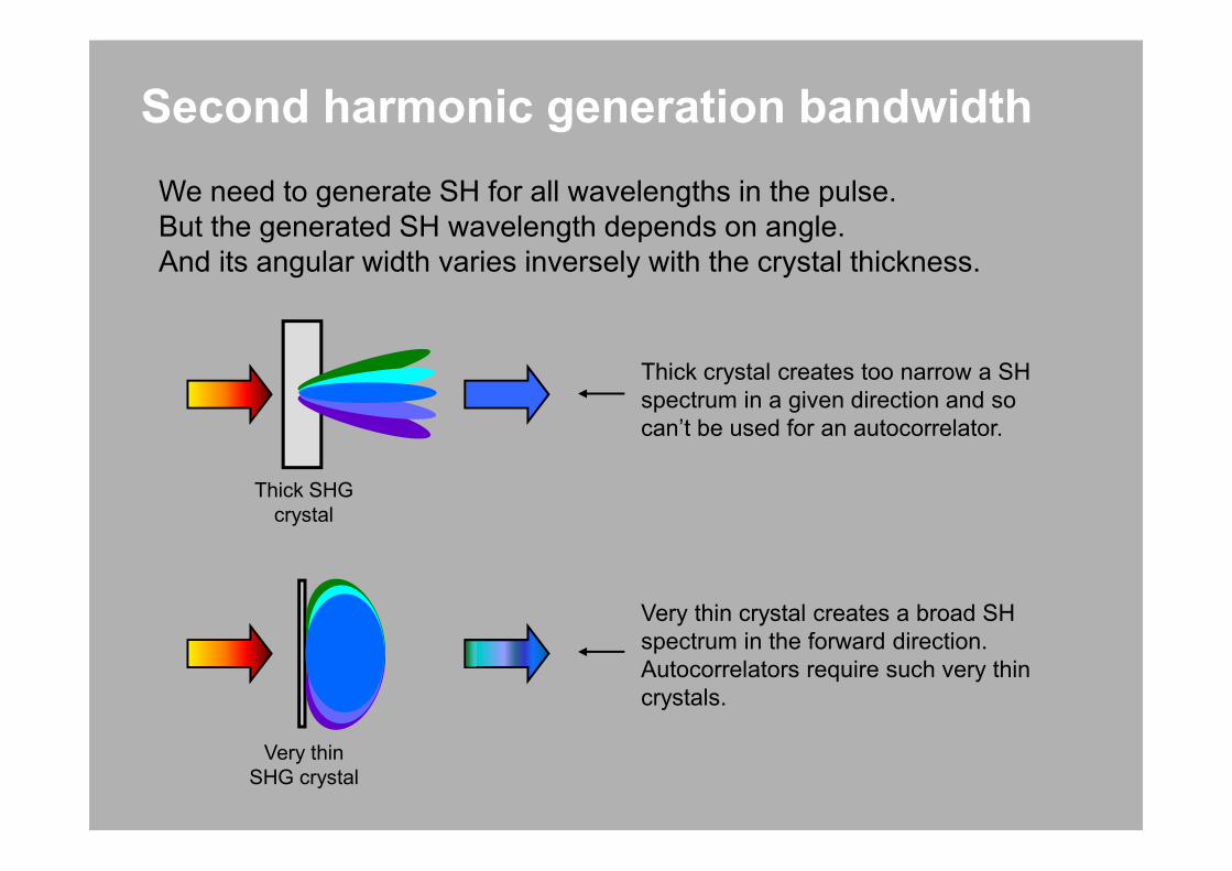
Thick crystal creates too narrow a SH

spectrum in a given direction and so

can’t be used for an autocorrelator.

Very thin crystal creates a broad SH

spectrum in the forward direction.

Autocorrelators require such very thin

crystals.

Very thin

SHG crystal

Thick SHG

crystal

We need to generate SH for all wavelengths in the pulse.

But the generated SH wavelength depends on angle.

And its angular width varies inversely with the crystal thickness.

Second harmonic generation bandwidth

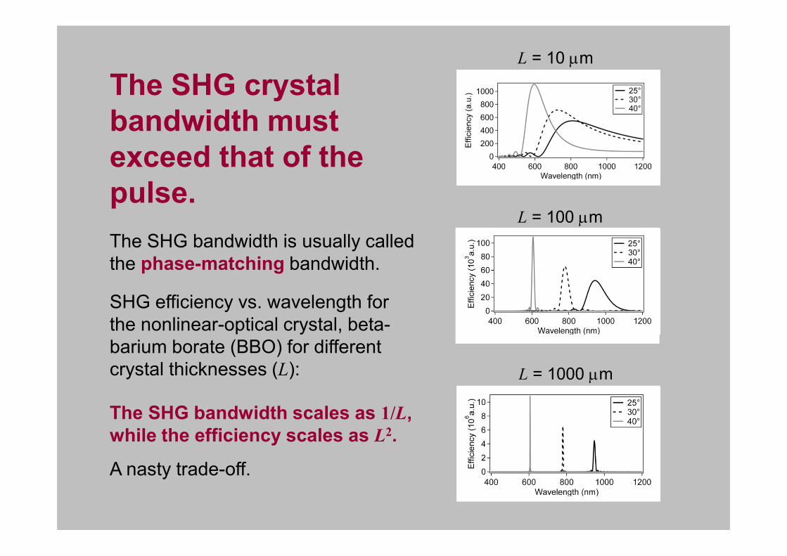
The SHG crystal

bandwidth must

exceed that of the

pulse.

SHG efficiency vs. wavelength for

the nonlinear-optical crystal, beta-

barium borate (BBO) for different

crystal thicknesses (L):

L = 10 µm

L = 100 µm

L = 1000 µm

The SHG bandwidth scales as 1/L,

while the efficiency scales as L2.

A nasty trade-off.

The SHG bandwidth is usually called

the phase-matching bandwidth.

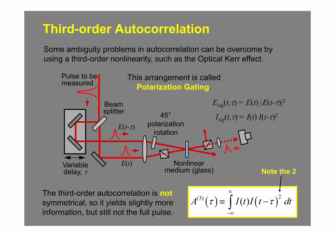
Third-order Autocorrelation

Nonlinearmedium (glass)

Pulse to be measured

Variable delay, τ

Beamsplitter

E(t)

E(t-τ)

Esig(t,τ) = E(t) |E(t-τ)|2

Some ambiguity problems in autocorrelation can be overcome by

using a third-order nonlinearity, such as the Optical Kerr effect.

45°

polarization

rotation

( ) ( )2(3) ( )A I t I t dtτ τ∞

−∞

≡ −∫

Isig(t,τ) = I(t) I(t-τ)2

The third-order autocorrelation is not

symmetrical, so it yields slightly more

information, but still not the full pulse.

This arrangement is called

Polarization Gating.

Note the 2

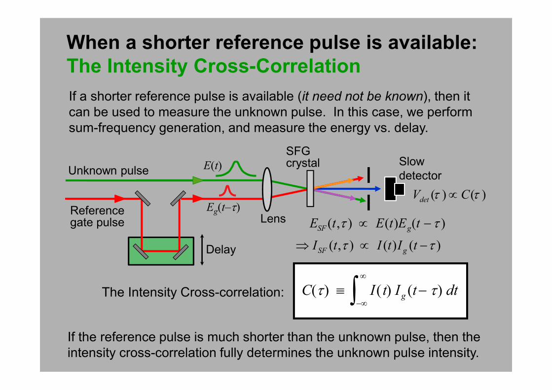
When a shorter reference pulse is available:

The Intensity Cross-Correlation

ESF (t,τ ) ∝ E(t)Eg(t −τ )

( , ) ( ) ( )SF gI t I t I tτ τ⇒ ∝ −

The Intensity Cross-correlation:

Delay

Unknown pulseSlow

detectorE(t)

Eg(t–τ)( ) ( )detV Cτ τ∝

SFGcrystal

LensReference gate pulse

C(τ) ≡ I(t) Ig (t− τ) dt−∞

∞

∫

If a shorter reference pulse is available (it need not be known), then it

can be used to measure the unknown pulse. In this case, we perform

sum-frequency generation, and measure the energy vs. delay.

If the reference pulse is much shorter than the unknown pulse, then the

intensity cross-correlation fully determines the unknown pulse intensity.

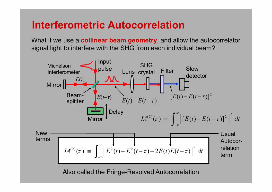
Michelson

Interferometer

Interferometric Autocorrelation

What if we use a collinear beam geometry, and allow the autocorrelator

signal light to interfere with the SHG from each individual beam?

2(2) 2( ) [ ( ) ( )]IA E t E t dtτ τ

∞

−∞≡ − −∫

2(2) 2 2( ) ( ) ( ) 2 ( ) ( )IA E t E t E t E t dtτ τ τ

∞

−∞≡ + − − −∫

Usual

Autocor-

relation

term

Newterms

Also called the Fringe-Resolved Autocorrelation

Filter Slow

detector

SHG

crystal

( ) ( )E t E t τ− −2[ ( ) ( )]E t E t τ− −

Lens

Beam-splitter

Input

pulse

Delay

Mirror

Mirror

E(t)

E(t–τ)

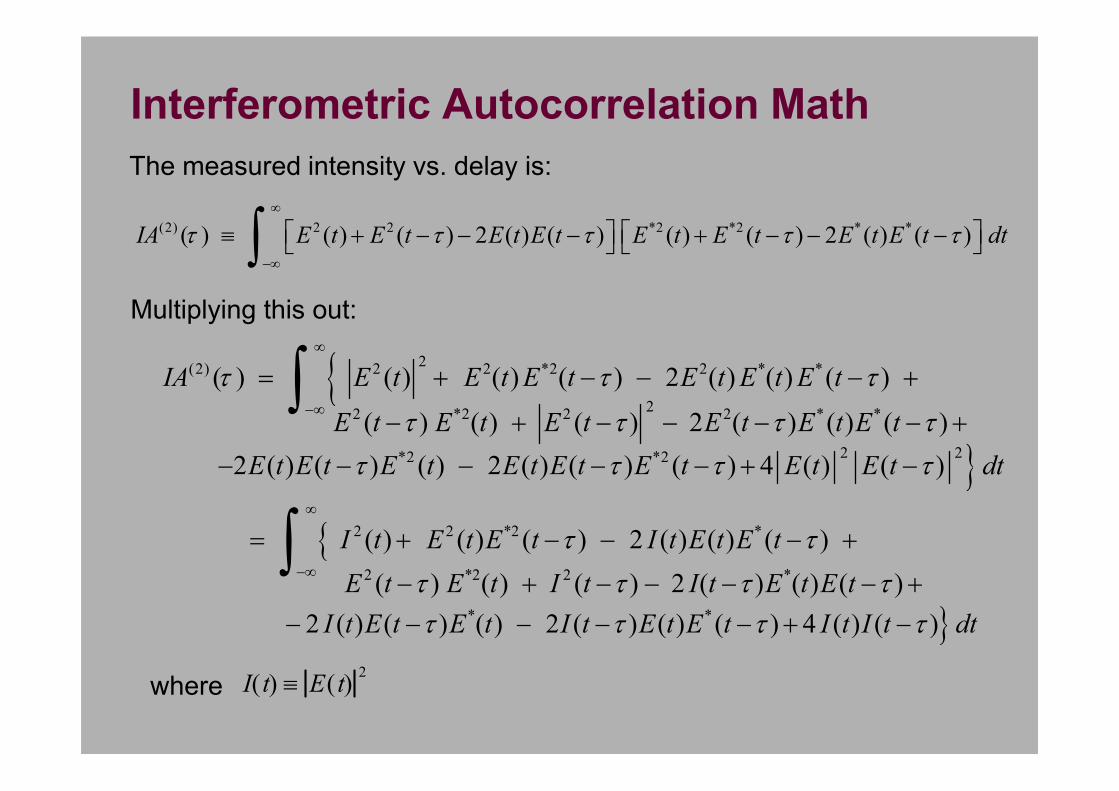
Interferometric Autocorrelation Math

The measured intensity vs. delay is:

(2) 2 2 *2 *2 * *( ) ( ) ( ) 2 ( ) ( ) ( ) ( ) 2 ( ) ( )IA E t E t E t E t E t E t E t E t dtτ τ τ τ τ∞

−∞

≡ + − − − + − − − ∫

{ 2(2) 2 2 *2 2 * *( ) ( ) ( ) ( ) 2 ( ) ( ) ( )IA E t E t E t E t E t E tτ τ τ

∞

−∞

= + − − − +∫Multiplying this out:

22 *2 2 2 * *( ) ( ) ( ) 2 ( ) ( ) ( )E t E t E t E t E t E tτ τ τ τ− + − − − − +

}2 2*2 *22 ( ) ( ) ( ) 2 ( ) ( ) ( ) 4 ( ) ( )E t E t E t E t E t E t E t E t dtτ τ τ τ− − − − − + −

{ 2 2 *2 *( ) ( ) ( ) 2 ( ) ( ) ( )I t E t E t I t E t E tτ τ∞

−∞

= + − − − +∫2 *2 2 *( ) ( ) ( ) 2 ( ) ( ) ( )E t E t I t I t E t E tτ τ τ τ− + − − − − +

}* *2 ( ) ( ) ( ) 2 ( ) ( ) ( ) 4 ( ) ( )I t E t E t I t E t E t I t I t dtτ τ τ τ− − − − − + −

where I(t) ≡ E(t)2

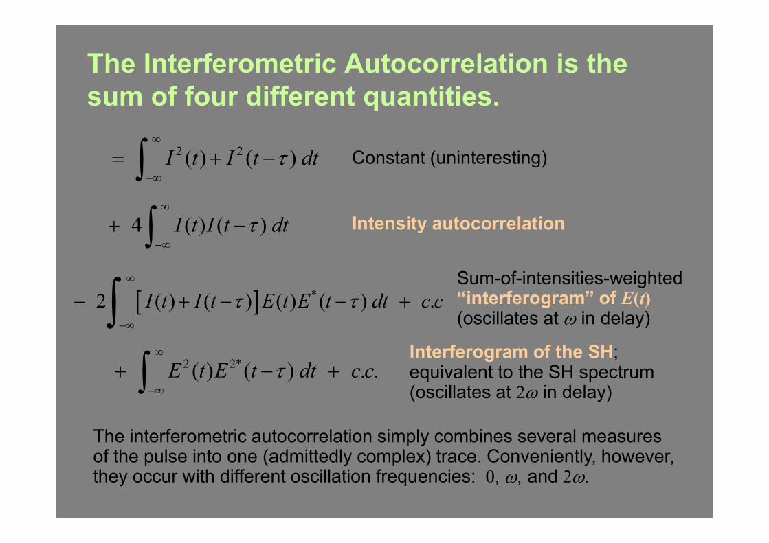
The Interferometric Autocorrelation is the

sum of four different quantities.

2 2( ) ( )I t I t dtτ∞

−∞= + −∫4 ( ) ( )I t I t dtτ

∞

−∞+ −∫

2 2*( ) ( ) . .E t E t dt c cτ∞

−∞+ − +∫

[ ] *2 ( ) ( ) ( ) ( ) .I t I t E t E t dt c cτ τ∞

−∞

− + − − +∫

Constant (uninteresting)

Sum-of-intensities-weighted ω“interferogram” of E(t) ω(oscillates at ω in delay)

Intensity autocorrelation

Interferogram of the SH;equivalent to the SH spectrum(oscillates at 2ω in delay)

The interferometric autocorrelation simply combines several measuresof the pulse into one (admittedly complex) trace. Conveniently, however,they occur with different oscillation frequencies: 0, ω, and 2ω.

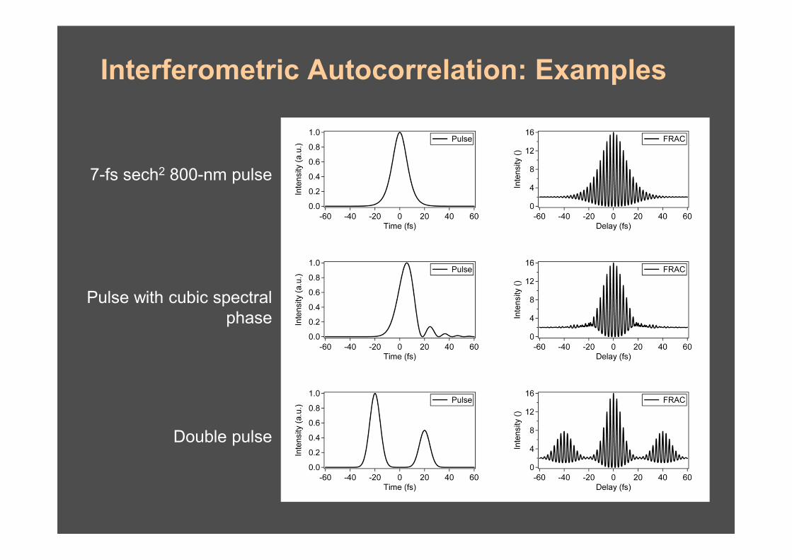
Interferometric Autocorrelation: Examples

7-fs sech2 800-nm pulse

Double pulse

Pulse with cubic spectral

phase

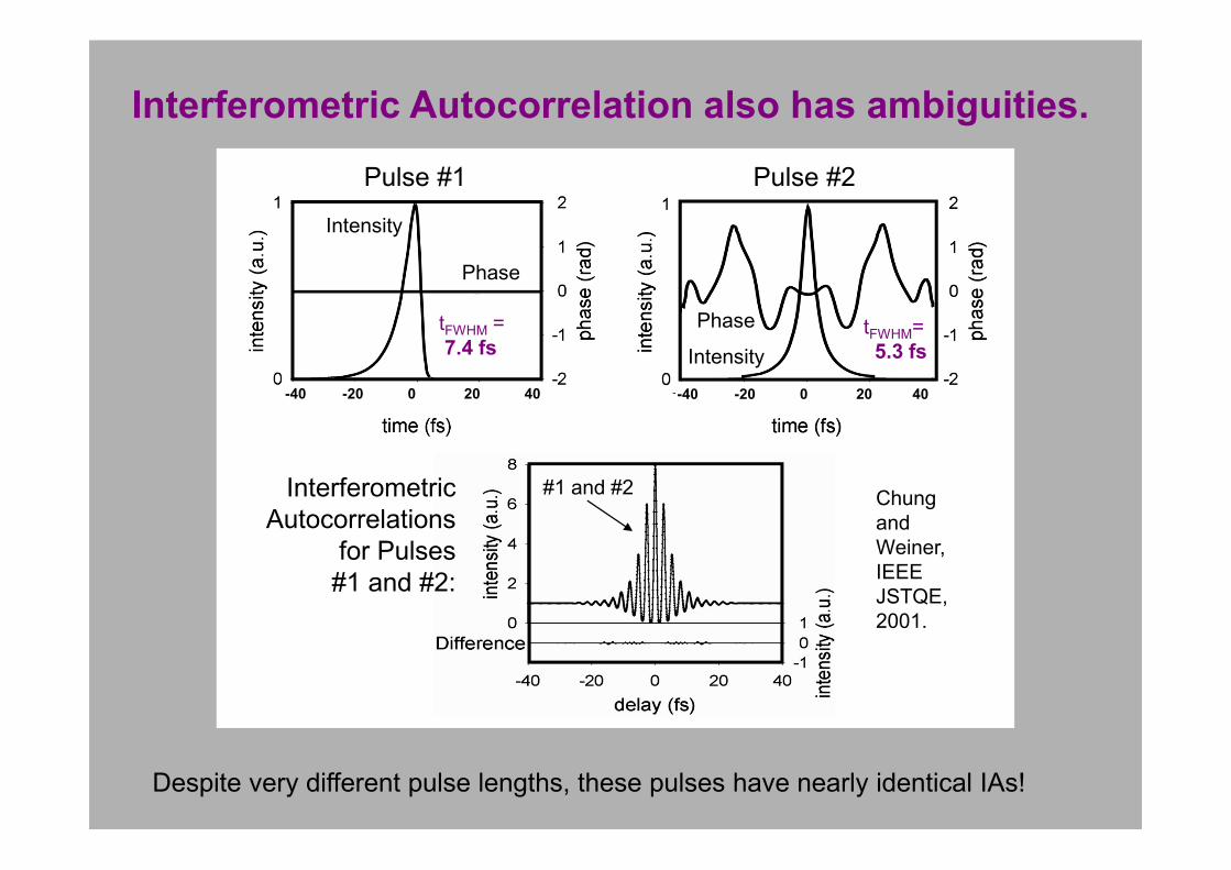
Pulse #2

Phase tFWHM=

5.3 fs

-40 -20 0 20 40

Intensity

Despite very different pulse lengths, these pulses have nearly identical IAs!

Chung

and

Weiner,

IEEE

JSTQE,

2001.

Interferometric Autocorrelation also has ambiguities.

Interferometric

Autocorrelations

for Pulses

#1 and #2:

#1 and #2

Pulse #1

Intensity

Phase

tFWHM =

7.4 fs

-40 -20 0 20 40

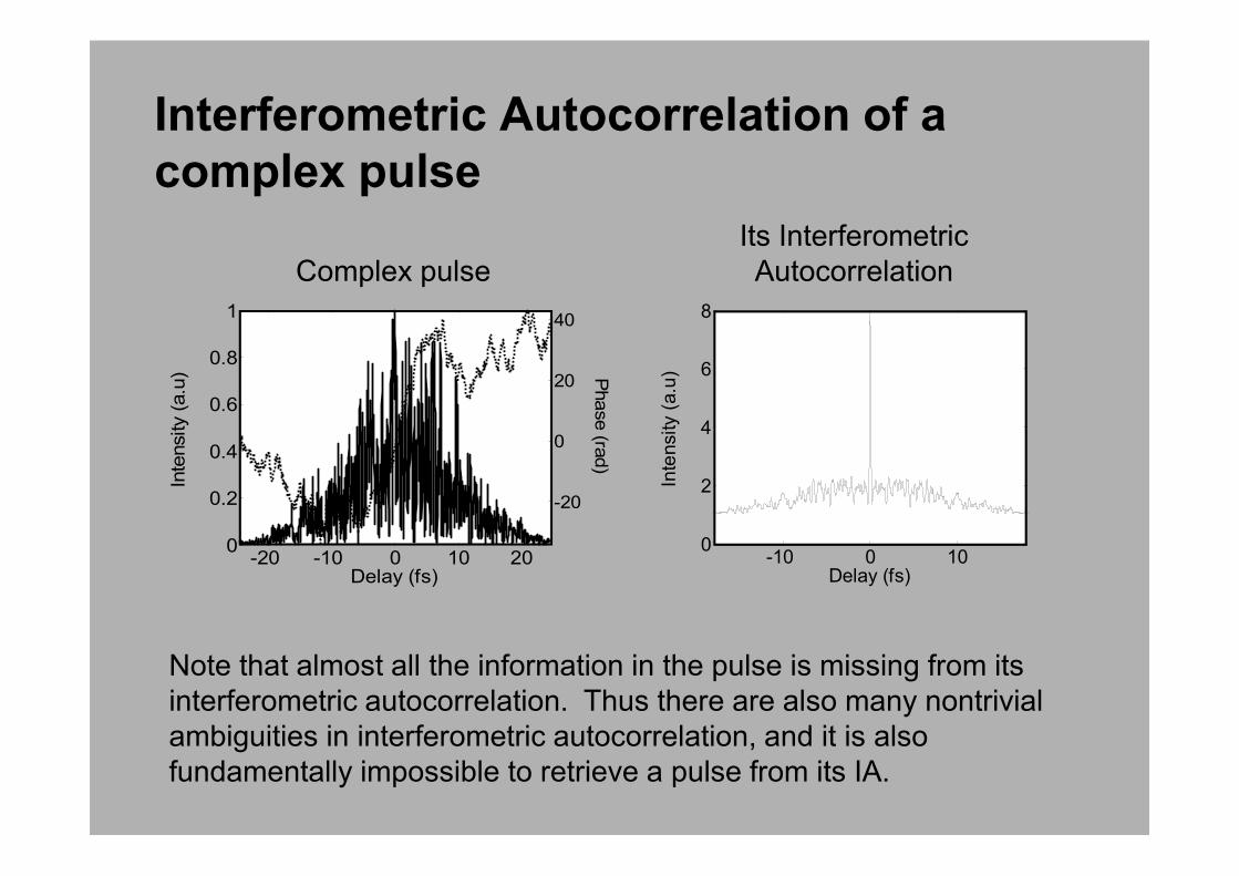
Interferometric Autocorrelation of a

complex pulse

Complex pulse

Its Interferometric

Autocorrelation

Note that almost all the information in the pulse is missing from its

interferometric autocorrelation. Thus there are also many nontrivial

ambiguities in interferometric autocorrelation, and it is also

fundamentally impossible to retrieve a pulse from its IA.

-20 -10 0 10 200

0.2

0.4

0.6

0.8

1

Inte

nsity (a.u

)

Delay (fs)

-20

0

20

40

Phase (ra

d)

-10 0 100

2

4

6

8

Delay (fs)

Inte

nsity (

a.u

)

Quiz: Which is the most difficult?

A. Time travel

B. World peace

C. Human teleportation

D. Retrieving a pulse from its intensity autocorrelation

or interferometric autocorrelation

The correct answer is D. Only it has been proven to be

fundamentally impossible. The others are hard, but,

as far as we know, they may be possible.