tabu search heuristic for minimizing the number of...
TRANSCRIPT

Tabu search heuristic for minimizingthe number of vehicles in VRPTW
by Jerome Baltzersen
January 29, 2010
Thesis adviser: Louise Kallehauge
Master project for Master of Science in Mathematics, Department ofMathematical Sciences, University of Copenhagen.

c© Jerome Baltzersen 2010
This thesis is printed using Computer Modern 11pt.Layout and typografy by the author using LATEX
Contents
Abstract iv
Resume v
Preface vi
1 Introduction 1
2 Basic theory 52.1 Heuristics and metaheuristics . . . . . . . . . . . . . . . . . . . . . . 5
2.1.1 Greedy heuristic . . . . . . . . . . . . . . . . . . . . . . . . . 62.1.2 Local search heuristic . . . . . . . . . . . . . . . . . . . . . . 6
2.2 Tabu search . . . . . . . . . . . . . . . . . . . . . . . . . . . . . . . . 72.2.1 Diversification and intensification . . . . . . . . . . . . . . . . 7
3 The vehicle routing problem with time windows 83.1 Formulation and setup of VRPTW . . . . . . . . . . . . . . . . . . . 83.2 The bin packaging relaxation of VRPTW . . . . . . . . . . . . . . . 9
3.2.1 The multi-dimensional bin packing problem . . . . . . . . . . 103.3 TSpack tabu search adaption . . . . . . . . . . . . . . . . . . . . . . 10
3.3.1 TSpack, main algorithm . . . . . . . . . . . . . . . . . . . . . 113.3.2 Filling function . . . . . . . . . . . . . . . . . . . . . . . . . . 123.3.3 Inner solver . . . . . . . . . . . . . . . . . . . . . . . . . . . . 133.3.4 Search algorithm . . . . . . . . . . . . . . . . . . . . . . . . . 133.3.5 Diversification algorithm . . . . . . . . . . . . . . . . . . . . . 153.3.6 Tabu list of TSpack . . . . . . . . . . . . . . . . . . . . . . . 173.3.7 Summary of interesting parameters for TSpack . . . . . . . . 18
3.4 Solomon heuristic . . . . . . . . . . . . . . . . . . . . . . . . . . . . . 18
4 Algorithm and program structure 204.1 Development platforms . . . . . . . . . . . . . . . . . . . . . . . . . . 204.2 Program and data structures . . . . . . . . . . . . . . . . . . . . . . 21
4.2.1 Class description . . . . . . . . . . . . . . . . . . . . . . . . . 214.2.2 GUI implementation . . . . . . . . . . . . . . . . . . . . . . . 21
ii

Contents
4.3 Test instances . . . . . . . . . . . . . . . . . . . . . . . . . . . . . . . 21
5 Computational results 235.1 Parameter tuning . . . . . . . . . . . . . . . . . . . . . . . . . . . . . 23
5.1.1 Filling function . . . . . . . . . . . . . . . . . . . . . . . . . . 245.1.2 TSpack algorithm . . . . . . . . . . . . . . . . . . . . . . . . 275.1.3 Summary of tuning phase . . . . . . . . . . . . . . . . . . . . 31
5.2 Performance on the Solomon instances . . . . . . . . . . . . . . . . . 31
6 Discussion 336.1 Adaption of algorithm . . . . . . . . . . . . . . . . . . . . . . . . . . 336.2 Tuning phase . . . . . . . . . . . . . . . . . . . . . . . . . . . . . . . 34
7 Conclusions 37
A Source Code 39A.1 TunedFillingFunction class . . . . . . . . . . . . . . . . . . . . . . . 39A.2 SolomonHeuristic class . . . . . . . . . . . . . . . . . . . . . . . . . . 40A.3 TabuListContainer class . . . . . . . . . . . . . . . . . . . . . . . . . 44A.4 TabuList class . . . . . . . . . . . . . . . . . . . . . . . . . . . . . . . 45
B Data 47B.1 Significant factors of filling function . . . . . . . . . . . . . . . . . . 47B.2 Tuning of search algorithm . . . . . . . . . . . . . . . . . . . . . . . 57
iii

Abstract
This thesis discusses a tabu search algorithm variant for solving the vehicle rout-ing problem with time windows (VRPTW). First, basic theory of heuristics andmetaheuristics are introduced. Thereafter the original algorithm used to solve binpackaging problems is discussed and adapted to the VRPTW setting.
The algorithm naturally focuses on the packaging dimension of the VRPTW andtries to empty a specific vehicle in order to minimize the number of vehicles in asolution. A key component of the algorithm is a so-called filling function tryingto identify vehicles from which all customers are easy removable. A tuning of thefilling function is performed and compared to the original filling function from the binpackaging setting. The tuned version performs significantly better on the Solomonbenchmark problems, but is still far from the best-known solutions.
The adaption of the algorithm seems promising and suggestions for further re-search and areas of interest are provided.
iv

Resume
Denne afhandling omhandler en variant af tabu-søgningsalgoritmer til at løse vehi-cle routing problemer med tidsvinduer (VRPTW). Indledningsvist introduceres dengrundliggende teori bag heuristikker og meta-heuristikker. Derefter diskuteres denoprindelige algoritme udviklet til at løse bin packaging problemer og denne tilpassesVRPTW omstændighederne.
Naturligt nok fokuserer algoritmen pa paknings-dimensionen af VRPTW-pro-blemet, og forsøger at tømme et udvalgt fartøj for derved at minimere antallet affartøjer i en løsning. En nøglekomponent i algoritmen er den sakaldte fylde-funktion,der forsøger at identificere de fartøjer, hvor alle kunder let kan flyttes. En tuningaf denne fylde-funktion gennemføres og sammenlignes med den oprindelige fylde-funktion fra pakningsproblemet. Den tunede fylde-funktion leverer signifikant bedreresultater paSolomons referenceproblemer, men er stadig langt fra de bedste kendteløsninger.
Tilpasningen af algoritmen virker lovende, og der gives forslag til videre forskningsamt interesseomrader.
v

Preface
This thesis is written as part of a Master of Science in pure mathematics at theUniversity of Copenhagen, even though it treats an applied field of mathematics,namely operations research. There is of course extensive use of mathematics in thisthesis, but it is not a typical definition-theorem-corollary setup known from abstractmathematics. Rather, aspects from computer science and algorithmic theory areused among others to solve a model of a real life problem. In order to get as faras possible with the applications of the powerful mathematical tools the theory ispresented rather than developed.
I would like to thank my adviser, Louise Kallehauge, for believing in me andposing a tough problem of applying an existing algorithm to a new area. Throughoutthe work on the thesis she, and often times her husband Brian Kallehauge as well,have patiently advised me, and helped me stay on track. Daniele Vigo, who originallysuggested the adaption of the algorithm to the VRPTW-problem, has kindle beensupervising the process and helping out whenever questions of doubt arose.
Finally, two friends deserves to be thanked. Michael Mc Donnell with his vastknowledge of Java and computer science in general has without hesitation helpedme whenever technical difficulties arose. Without him the code would be signif-icantly less elegant and on quite a few occasions technicalities would have stolenprecious time from the actual work. I would also like to thank Morten Hornbech.Despite being in the middle of finishing his own thesis and having a family to lookafter, he took time off to understand the problem, listen to my thoughts for furtherdevelopment, and provide a fresh perspective.
Jerome BaltzersenCopenhagen, January 2010
vi

CHAPTER 1
Introduction
An infamous problem in operations research is the travelling salesman problem(TSP) where a salesman wishes to visit a number of customers and return to hisor her home base traversing the shortest possible distance. The problem is simpleenough to present to a layman. But at the same time challenging enough to pose atough problem to the academic society.
The vehicle routing problem (VRP) has a fleet of vehicles located at a depot.These vehicles have to visit a number of customers and return to the depot usingthe fewest number of vehicles and/or travelling the shortest total distance. As suchit is a straight-forward generalization of the TSP and thus naturally attracts a lot ofacademic interest. Due to its more abstract nature compared to the TSP, techniquesof more complex nature are needed in order to attack the problem.
Further, the VRP is very relevant to the business world. A vast amount ofbusinesses face the task of visiting customers to make a delivery, perform a service,or what not. While the TSP is certainly relevant it is more often the case thatbusinesses have to attend to way more customers than what a single person/vehiclecan handle. Thus multiple “salesmen” are hired turning the problem into a VRP.
There are many adaptions and generalizations of the basic VRP and in whatfollows we are concerned with the variant further constraining the capacity of thevehicles, and imposing a time-window during which the visit has to be made. Sucha problem is called the (capacitated) vehicle routing problem with time windowsusually abbreviated VRPTW.
Whereas the TSP setting only has one natural objective, namely minimizingthe total distance traversed, the VRP has two natural objectives: One can try tominimize the total distance travelled or the number of vehicles used. There can be—and in realistic settings there usually is—a certain amount of correlation betweenthe two, but nevertheless it is important to realize that the two objectives are quitedifferent in nature. It is of course sensible, regardless of which objective is chosen, tokeep the other in mind as well. That is, for example, if two configurations uses thesame number of vehicles the one yielding the shorter total distance is to be preferred.
1

1 Introduction
Academics aside, these thoughts translates nicely into business objectives. Busi-nesses wishing to maximize profits are of course interested in minimizing costs givena certain level of revenue. Costs split into fixed and variable costs, which can beseen as the number of vehicles and the total distance travelled, respectively. Hav-ing an additional vehicle in one’s fleet adds to the fixed costs: you need to acquirethe vehicle, buy insurance, hire a driver, and so on. The variable costs come fromfuel consumption and wear on the vehicle per distance travelled. Again, regardlessof which approach a business wishes to focus on, they are ultimately interested inkeeping overall costs as low as possible and would therefore, for example, prefer theconfiguration with the smaller number of vehicles used given two configurations withthe same total distance travelled.
The business world has traditionally been more concerned with the minimizationof the number of vehicles used.
There might of course be further criteria to consider when solving a VRP-likeproblem. As an example of such the delivering company UPS prefers right turnsover left turns.1 It often times shaves off some distance travelled, but even whennot time is saved. As one article explains:
And at stop lights, making a right turn at an intersection tends to befaster than at a left turn, since you have only to wait for an opportunityto turn in one lane of traffic. You also have the option of ”right on red” inmost jurisdictions, unless otherwise indicated by traffic signs. ”So even ifyou didn’t save fuel, you’re going to move more quickly through a route.”
Other businesses specific challenges might pose other constraints providing aninteresting interplay between academia and business. What is important to a specificbusiness and how do we model this?
In this thesis the number of vehicles serves as primary objective. This decisionmakes it possible to use algorithms developed for a different class of problems as isexplained in the following.
To attack the problem an algorithm originally developed for the bin-packagingproblem by Vigo et al. [2] is adapted to the VRPTW-setting. In bin-packagingproblem it is tried to pack a number of spatial objects into as few and small bins aspossible. Vigo et al.’s algorithm locates a target bin and then tries successively toplace its contents among the other bins thereby reducing the total number of binsneeded if the entire contents are relocated.
In light of this, the VRP and its cousins can be viewed as a reformulation ofa packing problem: Given a set of customers how can we “pack” these into somevehicles? Each customer might have a unique “size” corresponding to a demand,and a vehicle has a spatial limit corresponding to its capacity constraint. While theanalogy is straightforward there is one important difference. Whereas the packingproblem has boxes into which the objects are packed and these boxes are free tomove around this does not hold for the VRP. The physical location of the customersis a given and cannot be manipulated. This is important when trying to relocate acustomer: Whereas a priori all bins are equally likely to absorb a new object not allvehicles are likely candidates for visiting the particular customer.
1See the following articles: http://multichannelmerchant.com/opsandfulfillment/advisor/
fuel_conserve/ and http://abcnews.go.com/WNT/story?id=3005890\&page=1
2

The details of the algorithm are explained in what follows and at this pointit suffices to remark that it incorporates the use of a tabu list to prevent cycling,and a diversification procedure. The intensification process is a bi-product of thesearch algorithm used. To assess the effectiveness of the algorithm the Solomoninstances [7] are used as benchmark, while a selected few are used for parametertuning. Performance is compared to the best known solution as well as solutionsfound using an approach mimicking Vigo et al.’s. The latter is done to give a feelingof the success of adopting the algorithm the VRPTW-problem.
In contrast to the original code written by Vigo et al. in C++, I have chosenJava and a purely object oriented approach. The choice of Java is due to its cross-platform capabilities easing further development of others regardless of platform.As this thesis demonstrates, the approach developed by Vigo et al. for the bin-packing problem can also be adopted with success to attack various other problemswhen reformulated as packaging problems. These reformulation might have specificstructures allowing us to increase the efficiency of the algorithm, but rather thanhaving to rewrite the code from scratch each time the object oriented approachallows one to replaces the problem specific objects and re-run the code.
Further, it is also easy to add a user interface such as graphic representation ofthe algorithm. A good graphic representation aids a researcher in understanding theunderlying dynamics of the algorithm and also provides students with an additionallearning tool thereby increasing understanding. One will be able to step through thealgorithm and see how a target vehicle is chosen and attempts to empty it are made.Many factors can be used to determine the target vehicle, but it is often extremelydifficult to say anything about the significance or even the sign (!) of correlationof the factors. Having a graphical representation allows the human mind to use itspattern-recognizing abilities in addition to one’s gut feeling and analytical skills.
Summing up, the author believes that the object oriented approach simplifies theuse and further development of the code. As pointed out by Cordeau and Laportein [5]
[...] the research community is used to assessing heuristics with respectto accuracy and speed alone, but simplicity and flexibility are often ne-glected. Yet these two attributes are essential to adoption by end-usersand should be central to the design of the next generation of algorithms.
Finally, besides making the code more approachable, it also adds the possibilityof using framework specific capabilities such as unit testing of code, and designpatterns. Excerpts of the source code are found in Appendix A, while the full sourcecode is available from http://baltzersen.info/vrp.php.
Despite a lot of time and energy being put into the tuning section, it quicklybecame clear that a rigorous tuning and analysis was beyond the scope of thisthesis. Instead a combination of statistical analysis and gut-feeling has been usedto tune the parameters. Further, not all parameters have been tuned, but rather aprioritized order has been established. Not being able to perform a rigorous tuning,this thesis at least provides a blueprint of how such one could be carried out.
After the tuning phase and with the results on the Solomon instances this thesissums up its finding and concludes. The conclusion includes an assessment of thevalue of further research and how one could approach it. It is found that albeitresults being relatively far from the best known, further research is likely to befruitful.
3

1 Introduction
This thesis consists of Chapter 2 introducing the basic theory needed to under-stand the algorithm. While the chapter is written for a general audience the selec-tion of material has been dictated by the components of what follows and efforts tokeep it brief are made. Chapter 3 deals with the VRP in detail: its formulation, aproblem-specific heuristic, and describing the algorithm by Vigo et al. and its adap-tion to VRP. The implementation of the algorithm, comments on the specific code,and other computer science issues are briefly presented and discussed in Chapter 4.The computational results are listed and discussed in Chapter 5, while Chapter 6discusses the results. Finally, conclusions are gathered in Chapter 7.
4

CHAPTER 2
Basic theory
This chapter deals with basic theory needed in the remainder of the thesis. We dis-cuss heuristics and metaheuristics providing examples of both in particular focusingon the tabu search. The chapter aims to be unrelated to the specific discussion, butis of course developed keeping what follows in mind.
The exposition is based on a textbook by Wolsey [3]. Additional referencesinclude Glover [4], who originally proposed and coined the term tabu search, andCordeau and Laporte who provide a useful survey [5].
2.1 Heuristics and metaheuristics
A vast majority of the problems of interest to both the academic society and thebusiness world are infeasible to solve exact for all but the smallest instances. Thismotivates the use of heuristics. A heuristic should be thought of as an algorithmyielding a “good,” usually feasible, solution rapidly—that is typically within someseconds or, on rare occasions, minutes. For some problems that can indeed be solvedexactly albeit requiring a lot of computation time one would still choose a heuristicin order to quickly find a satisfactory solution. Heuristics can be thought of as a wayto increasing computational efficiency potentially at the cost of solution accuracy.
Coincidentally, a majority of the problems of interest to the business world areinfeasible to solve exact,1 which spawned a great interest in heuristics. In studyinga heuristics interesting questions include:
• Is it possible a priori to say how close to the optimal solution our solution willbe?
• Is it possible a priori to say how close to the optimal solution our solution onaverage will be?
Depending on the problem, the quality of a heuristic solution is sometimes ques-tioned, while at other times any feasible solution will suffice. The latter criterion
1They are non-polynomial time complete, NPC.
5

2 Basic theory
is often used even in problems where the quality of the solution is of interest. A(meta)heuristics is then used to improve the known solution. Meta-heuristics relyon an initial solution, called the incumbent, to get started.
2.1.1 Greedy heuristic
Two classical heuristics are the greedy heuristic and the local search heuristic. Thegreedy heuristic attempts to construct a feasible solution from scratch. The ideais fairly simple and best illustrated via an example. Considering the (symmetric)traveling salesman problem (STSP) we wish to construct a greedy solution: Startingat the office, we simply choose the closest customer at each iteration until all cus-tomers are visited upon which we return to the office calling it the day. The greedyheuristic thus sacrifices the big picture and always chooses the immediate “best” op-tion. Formally, a greedy algorithm needs, among others, a function to determine the“best” option; in this particular case the Euclidean distance between two customers.
While it is easy to construct STSP instances for which the greedy algorithmalways provides a feasible, but sub-optimal solution there are problems for whichthe greedy algorithm will always return the optimal solution. Problems for which nofeasible solution is found, even though one exists, are also possible. The followingare examples of both.
Consider the change problem: A customer needs to get a change of $0.41 and wewish to use as few coins as possible. A greedy algorithm, in this case our salesclerk,first picks a quarter, then a dime, a nickel, and finally a penny. This is both afeasible and optimal solution. But consider instead a monetary system in which theavailable coins are 25-cent, 10-cent and 4-cent. In this case the salesclerk would failto produce a feasible solution even though one exists.2 A similar problem could arisein the VRP setting where one could imagine that feasible solutions exists, but noneof them found by a greedy algorithm.
2.1.2 Local search heuristic
We now turn to the local search heuristic. Given an incumbent, S, the local searchdefines a neighborhood of solutions around the incumbent denoted by Q(S) andafter examining Q(S) it moves to a new and better solution. The choice is basedsolely on information about the solutions in the neighborhood, hence the name localsearch. Typically, a neighborhood has more than one solution and if the choice isbased entirely on local maximization the heuristic is sometimes referred to as a hillclimber. Termination is usually controlled by either computation time or when onehas reached a local optimum. Obviously, in both cases the solution is most likely nota global optimum as the examined neighborhood may be very far from the globaloptimum.
For such an algorithm, we need to define Q(S) for all S and a goal functiondenoted by f : N → R, where N denotes the space of solutions. The goal function
2The salesclerk would pick a quarter, a dime and then be stuck where as a quarter and four 4-cents would yield $0.41. This example is of course a reformulation of the well-known knapsackproblem.
6

2.2 Tabu search
is used to evaluate a particular solution and often one uses
f(S) =
{c(S) if S is feasible,∞ if S is infeasible,
where c simple denotes the cost/objective function of the particular problem. Whichneighborhood-constructing function Q is used is problem specific.
2.2 Tabu search
Both the greedy heuristic and the local search have their limitations, which is whymetaheuristics are introduced. “Meta” is Greek and translates into something like“higher level” or “beyond.” The term “metaheuristic” was first coined by Glover in1986 in his article on tabu search [4]. The basic idea of a metaheuristic is to guide aheuristic to avoid its inherent pitfalls. For example, where the local search efficientlylocates local minima it lacks the broader perspective, which a meta-heuristic setsout to repair. a metaheuristic therefore needs extensive knowledge of the heuristicitself.
When our heuristic only operates locally it is natural to pose the question of howto escape a local optimum in order to shift the neighborhood and discover a bettersolution. A first idea would be to allow moving to a solution even though it is worsethan our local optimum. Doing so, the risk of cycling is faced, that is moving fromS0 to S1 only to move back to S0 again and so on and so forth. Tabu search triesto avoid such cycling by marking certain solutions as tabu meaning that one is notallowed to return to the solution.
A tabu list is kept, which can be thought of as truncated list of all previousincumbents. Keeping a complete list and checking if a given solution is already listedis computationally inefficient. One parameter for the tabu search includes the lengthof the list. If too short, cycling is not prevented, while if too long computationalefficiency suffers. The literature often cites a length of seven as a good trade off.The tabu list is sometimes referred to as short term memory.
Other parameters to be defined are, analogously to the local search heuristic,how Q(S) is chosen as well as what termination criterion should be used. A fixednumber of iterations or a certain number of iterations without improvement are oftenchosen, while a time limit can also be used.
2.2.1 Diversification and intensification
The tabu search uses additional ingredients, diversification and intensification, re-spectively, needed to build a successful algorithm. Intensification is an algorithmthat tries to find common characteristics among the good solutions found so farin order to intensify the search for an optimal solution in solutions sharing thesecharacteristics.
In contrast, diversification looks to investigate solutions with very different prop-erties from those already investigated in order to escape a local optimum. One wayof achieving this, assuming a minimization problem, would be to decrease the objec-tive function for solutions far from the current solution, while increasing it for thosewho are close. Diversification is also known as long term memory.
7

CHAPTER 3
The vehicle routing problem with time windows
This thesis focuses on using a heuristic, TSPack, originally developed in 2004 byVigo et al. [2] for solving bin packaging problems. The algorithm is adapted to theVRP problem and tries to minimize the number of vehicles used. The only problem-specific part of the algorithm is an inner solver used to analyze smaller subsets ofcustomers. We have chosen to use a heuristic proposed by Solomon in 1987 [6] asinner solver.
In this chapter are introduced the formulation of VRP, the TSPack algorithm,and the Solomon heuristic. We focus on explaining the algorithms in detail andmotivate each choice. The code of the algorithm has been modified for variousreasons. Some changes stem from the fact that implementing the code in Java isslightly different from a C++ implementation, while the fact that the code is objectoriented implies changes as well.
3.1 Formulation and setup of VRPTW
We wish to present a mathematical formulation of the VRPTW and begin withan intuitive understanding of the problem before turning to a rigorous formulation.Vehicles start at a depot have to visit a given number of customers placed on amap. Each customer has a continuous time window during which the visit must beinitiated and a certain demand for goods. The fleet consists of identical vehicleswith a capacity constraint. All the vehicles have to return to the depot before afixed point of time. The time it takes to travel between two customers is equal tothe distance between them; such a problem is sometimes referred to as a Euclideanproblem.
In order to formalize this, we consider a weighted graph with arcs A referred toas (i, j). To ease the formulation the graph contains a start depot denoted by 0,and an terminal depot denoted by n+ 1 both at the same location. Doing so allowsus to have unused vehicles travel between the two depots—corresponding to neverleaving the actual depot in the first place. Further, some of the constraints in theformulation become neater this way.
8

3.2 The bin packaging relaxation of VRPTW
The set of vehicles is denoted by K, N = {0, . . . , n+ 1} is the set of all nodes—customers as well as both depots—while C is the set of the customers only. Customeri’s service interval is denoted by [ai, bi], ai, bi ∈ R+, while the demand is denoteddi. tij is the time it takes to travel between customer i and j; here, as mentioned,simply the distance between the two. sik ∈ R+ is the time a vehicle k begins to servecustomer i if k visits i. If not, sik is meaningless and simply assigned an arbitraryvalue satisfying the constraints below. Finally, the formulation uses binary variablesxijk defined by
xijk =
1 (i, j) ∈ A is used by vehicle k,1 i = j, and0 otherwise.
The formulation as an linear integer program can now be written as:
z := min∑k∈K
∑j∈C
x0jk (3.1)
subject to∑k∈K
∑j∈C
xijk = 1, ∀i ∈ N (3.2)
∑j∈C
x0jk = 1, ∀k ∈ K (3.3)
∑i∈C
xihk −∑j∈C
xhjk = 0, ∀h ∈ N, ∀k ∈ K (3.4)
∑i∈C
xi,n+1,k = 1, ∀k ∈ K (3.5)∑i∈N
di
∑j∈C
xijk ≤ q, ∀k ∈ K (3.6)
sik + tij − (1− xijk)(bi − aj) ≤ sjk, ∀i, j ∈ N, ∀k ∈ K (3.7)ai ≤ sik ≤ bi, ∀i ∈ N, ∀k ∈ K (3.8)xijk ∈ {0, 1}, ∀(i, j) ∈ A,∀k ∈ K (3.9)sij ∈ Z+, ∀i ∈ N, ∀k ∈ K (3.10)
The objective function in (3.1) expresses the fact that we wish to minimize thenumbers of vehicles leaving the start depot to visit a customer. (3.2) makes surethat each customer is visited exactly once, while (3.3)-(3.5) makes sure that eachroute is a connected path actually beginning in the start depot and ending in theterminal depot (for balance). The capacity constraint is given by (3.6), while (3.7)and (3.8) deal with the time window constraint. (3.9) and (3.10) define the solutionspace.
The complexity of this problem is NP-hard, which easily follows from the factthat the TSP, being a special case, is NP-hard.
3.2 The bin packaging relaxation of VRPTW
When solving the VRPTW there are three subproblems to keep in mind: the capacityconstraint on the vehicles, the geographical placement of the customers, and the timeintervals for the service times of each customer. Having to visit customers in the
9

3 The vehicle routing problem with time windows
shortest possible manner is similar to the TSP, while having to visit them in certaintime intervals corresponds to a scheduling problem where one wants to minimizethe tardiness of a set of machines. The third ingredient of the VRPTW is whatof particular interest to us in this case, namely trying to pack the demand of thecustomers into vehicles with a fixed capacity.
Viewing the problem as such, it is very similar to a packaging problem as theone considered by Vigo et al. And it is this similarity that we are concerned within the remainder of this thesis. The idea is to take the approach proved successfulby Vigo et al. in the packaging setting, adapting it to solving a VRPTW, and thenrefine it by using the additional structure given in a VRPTW setting.
In order to give the reader a better understanding of this, we briefly introducethe packaging problem considered by Vigo et al. A more rigorous treatment is in[2].
3.2.1 The multi-dimensional bin packing problem
We present the three-dimensional bin packing problem (3BP). Vigo et al.’s algorithmis designed to solve both the two and three dimensional case, but as the first is asimple special case of the latter, we focus our efforts.
Consider a boxed item j, j = 1, . . . , n with dimensions wj , hj , and dj , andidentical bins with dimension W , H, and D. The simplest variant of the problem isto pack the n items in as few bins as possible. Additional constraints might requirethat the boxes have a certain orientation (relevant, for example, for containers ofliquid). The same framework can be applied in cutting contexts. One starts outwith a big block of material which needs to be divided into n smaller blocks. In sucha context a further constraint might be that it is guillotine cutable, that is that anycut is from edge to edge and parallel to the edges of the initial block.
It pays to keep the original context in mind as some of our vocabulary is fromthe original paper including, obviously, the name of the algorithm: TSpack. This isdone to make comparison easy, but also to aid intuition.
3.3 TSpack tabu search adaption
The algorithm by Vigo et al. [2] chiefly consists of five parts described in detailbelow:
• Main algorithm, which is controls the flow of the program. Referred to asTSpack,
• Filling function controlling which vehicle to try to empty,
• Inner solver, denoted by A, returning solutions to subproblems,
• Search algorithm, which searches the neighborhood, and
• Diversification algorithm.
These parts are tightly weaved together and the algorithm relies on all. Unfor-tunately, it is not possible to introduce all concepts simultaneously and the readerhas to live with the fact that a section might refer to a discussion of a following
10

3.3 TSpack tabu search adaption
section. To aid comprehension of the concepts much effort has put towards makingit abundantly clear whenever this is the case.
Note that, the algorithm uses a non-standard tabu list, which is described inSection 3.3.6. To conclude the section parameters of interest are summarized.
3.3.1 TSpack, main algorithm
A bit unusual for a tabu search algorithm, TSpack itself does not directly striveto perform any local improvements, but rather relies heavily on an inner solverdescribed in detail in Section 3.3.3. This inner solver is called repeatedly throughoutthe execution of the algorithm and any change to the solution is made by replacingthe configuration of a specific subset of customers S by A(S).
Keeping in mind that the algorithm strives to minimize the number of vehiclesused in visiting the customers, the idea is to determine a vehicle—referred to asthe target vehicle—which we will try to eliminate by reassigning customers. Thecriterion used is based on a filling function, φ, such that the target vehicle is thearg optimumφ(v) over all active vehicles v.1 The filling function is described inSection 3.3.2.
The first incumbent solution, A0, is a user controlled parameter. This is ana-lyzed, a target vehicle is identified, and control is passed on to the search algorithm.The search algorithm potentially decreases the number of vehicles by replacing thecustomers of the target vehicle. At some point, though, all its options have beenexplored and a diversification process is initiated.
This procedure is repeated until an iteration limit, l_max, has been reached or,alternatively, a time limit can be used. Before beginning the algorithm a lowerbound L is calculated, which in our case is simply the aggregated demand of thecustomers divided by the vehicle capacity. Throughout the algorithm it is checkedwhether the lower bound is reached and if so the algorithm terminates.2
To understand the dynamics of the algorithm it is vital to note that one iterationof the algorithm corresponds to the search algorithm completing one search of theneighborhood, and a request for diversification. The entire procedure may in pseudocode be written as
TSpack (){int lowerBound = max(1, (int) ceil(customers.getTotalDemand()/ vehicleCapacity));
vehiclesUsed = solution.numberOfVehiclesUsed();if (vehiclesUsed == lowerBound)return solution;
d = 1;targetVehicle = Utilities.determineTargetVehicle(solution);
1Where arg optimum is the operator that returns the argument for a given function such that itis optimized, that is either maximized or minimized depending on the context.
2In practice, the author has never seen the lower bound being reached and in doing so causetermination. If this would happen one could consider removing the piece of code as one mightbe able to find a solution with the same number of active vehicles and a shorter total distance.This is a good example of how additional structure in the VRPTW setting influences the code.As the check is computationally very cheap removing the code does not affect performance.
11

3 The vehicle routing problem with time windows
int iteration = 1;while (iteration <= iterationLimit){if (diversify)Diversification();
diversify = false;k = 1;while (!diversify && vehiclesUsed > lowerBound){int k_in = k;Search();if (k <= k_in)targetVehicle = Utilities.determineTargetVehicle(solution, d);
}if (vehiclesUsed == lowerBound)return solution;
iteration++;}return optimalSolution;
}
3.3.2 Filling function
As described in Section 3.3.1, the filling function is primarily used to pick the targetvehicle. One can think of many factors to consider, but the overall purpose is todesign a function that picks the vehicle whose customers is relocated easily suchthat the vehicle can be eliminated. These factors could involve number of customersvisited, used capacity, arrival times structure, and more. More generally, the fillingfunction can depend on factors involving one or more dimensions of the VRPTW,and either be intrinsic—only involving the vehicle at hand—or extrinsic—involvingone or multiple pieces of information from other vehicles. This is summarized andexemplified in Table 3.1.
Note, that this classification would also be applicable to the BPP case. Naturally,due to the absence of two of the dimensions factors belonging to these are of littleuse, but consider the capacity of other boxes could be relevant.
The filling function is defined for any vehicle and thereby orders the vehicles.While the search algorithm tries to empty the target vehicles using the inner solverit is of paramount importance to pick the right target vehicles. No matter how wellthe inner solver relocates the customers of the target vehicle we do not move closerto an optimal solution if the wrong target vehicles are picked on a consistent basis.Much effort is therefore put into finding a suitable filling function, albeit it alwaysto a certain degree depends on the problem at hand.
As there is no such thing as a generic optimal filling function our diversificationprocedure described in Section 3.3.5 to some extent aids the choice of the correcttarget vehicle. The filling function is naturally a parameter, which is itself oftenparameterized.3
3The filling function originally used for the bin packing problem for the items Si in bin i is
φα(Si) = αP
j∈Sivj
V− |Si|
nwhere vj is the size of the item (area or volume), V is the total size
12

3.3 TSpack tabu search adaption
Intrinsic factors Extrinsic factors
Capacity • Capacity used by parti-cular vehicle,• Distribution of capacity
used among individualcustomers.
• Other vehicles with ex-cess capacity,• Clusters of customers
high/low in demand.
Arrival times • Waiting time,• Size of gaps in arrival
times.
• Other vehicles startinglate or ending soon.
Geography • Distance between visi-ted customers.
• Other vehicles passingnearby,• Isolated customers (seed
customers).
Table 3.1: Summary of the nature of potential factors for a filling function. The factors aresplit into each of the three dimensions for the VRPTW (vertical) and whetherthey involve additional vehicles or not (horizontal). Examples of factors are keptvery abstract.
3.3.3 Inner solver
The inner solver is denoted by A and for any subset of customers S the correspondingsolution is denoted by A(S). Formally, A(S) can both refer to the solution itself andthe number of vehicles used in the particular solution. As this is always clear fromthe context no additional notation is introduced.
There is nothing that dictates whether the inner solver should be a heuristic oran exact solver. There are, though, several things to keep in mind before decidingon which solver to use. The solver is run extremely often and runtime is therefore amajor factor. As will become clear shortly, the size subset of customers consideredvery much depends on the size of the neighborhood currently being searched.
For a small number of customers it might be feasible to use an exact methodwhere as larger subsets of customers are naturally best handled by heuristics. Thereare no limitations to how the inner solver can be chosen; one interesting approachcould be to have it solve small instances exactly while using a heuristic for largerinstances.
3.3.4 Search algorithm
The search algorithm is the most complex part, both conceptually as well as imple-mentation wise. It is also this algorithm that incorporates the use of the tabu listdescribed in Section 3.3.6.
As the aim of the algorithm is to empty the target vehicle each of its customersis considered in turn and tried to be placed on another route. A crucial ingredientin this relocation of customers is the size of the neighborhood denoted by k, which
available, n the number of bins, and α > 0 a parameter.
13

3 The vehicle routing problem with time windows
translates as follows: Consider the set of vehicles excluding the target vehicle. Thena k-tuple of these vehicles are considered. Their customers and the specific customerto be moved are put in a set S for which a new solution, A(S), is produced usingthe inner solver A. This solution is analyzed and further behavior is divided intothree cases.
Each of the three cases has to decide whether or not to execute the move and howto update the k value. Executing a move means that the current configuration of thek vehicles considered is replaced by the new configuration. It does not necessarilyaffect the best solution found so far as it is stored separately, but the two are ofcourse compared and the best found solution updated accordingly.
As explained in Section 3.3.6 a real number called penalty is used in Case 2 and3. It is initialized to ∞ and not changed in Case 2. Case 3 is treated below.
Case 1: A(S) < k This case is straightforward and no tabu list is consulted. If,beginning with k vehicles, it is possible to add a customer and obtain a configurationwith strictly fewer than k vehicles, the the overall number of vehicles is immediatelyreduced by 1. The move is executed, and k is reduced by 1 unless k = 1 in whichcase it is left unchanged, that is k = max{1, k − 1}. Control is returned to TSpack.
Case 2: A(S) = k If the customer considered, j, is the last visited by the targetvehicle it means that a configuration has been found where the customers from thek-tuple and j can be visited using k vehicles. This leaves the target vehicle withoutassignments and hence cuts a vehicle. The move is therefore executed and k isadjusted as above: k = max{1, k − 1}.
Otherwise the number of vehicles stays the same: The target vehicle remainsand the k vehicles originally considered are all still active. At first, it might seempromising to move a customer away from the target vehicle without increasing thetotal number of vehicles. One might wish to go ahead and execute the move rightaway, but on second thought there is no guarantee that this will be an overallimprovement. It could easily be that no further customers could be removed fromthe target vehicle, control would return to TSpack, and a new target vehicle wouldbe identified. This might very well be the vehicle to which we have just added thecustomer and we might end up moving the customer back.
This is exactly the kind of cycling described in Section 2.2 and therefore a tabulist is introduced. It is first checked if the move is tabu: If so, the next k-tuple isconsidered, but if not the move is executed and control returns to the main algorithm.
Note that even if the move is executed k is kept unchanged. We have not de-creased the numbers of active vehicles, but have only taken an uncertain step towardsa potential reduction. There is no reason to believe that reductions would be foundin the setting of a smaller neighborhood, which we have previously searched.
Case 3: A(S) = k + 1 and k > 1 At first glance this is a less attractive situ-ation. Unless the specific customer is the last being visited by the target vehiclean additional vehicle is needed. Nevertheless, we allow such a move under certaincircumstances.
Consider the set of the k+1 vehicles used in A(S) and determine the local targetvehicle t for this set in a similar manner to how it is done by the main algorithm.
14

3.3 TSpack tabu search adaption
Considering the set T := (St \ {j}) ∪ St, where j is the current customer and tthe original target vehicle. T is the residual customers of the target vehicle plusthe local target vehicle’s customers. If the inner solver finds a solution for this setthat only uses one vehicle, that is A(T ) = 1, a new move is obtained. This movestill uses k + 1 vehicles, but the target vehicle t is left with a single customer tovisit. Combining A(T ) with A(S) this last customer is removed as well and we havesucceeded in emptying the target vehicle.
Suddenly, such a move seems not good, but at least promising at the same levelas Case 2. It is easy imaginable that several such moves could arise during thesearch of a neighborhood of fixed size, and we therefore decide to store the moveand evaluate it against its peers. For each such moves that is not tabu an entitydenoted by penalty is calculated. The original solution S has been changed suchthat the local target vehicle t has been removed and instead the one vehicle makingup T has been added. The minimum of the filling function over this set of thesevehicles and store this number as the penalty. In formulae it reads
penalty := minM∪T{φ(·)}, (3.11)
where M is the set of vehicles from the original solution excluding t. Hereafter thecode does not return, but rather the search continues in hope of stumbling upon aCase 1 or 2 move.
When having searched the entire neighborhood without returning to the mainalgorithm, that is not having executed Case 1 or 2, it is checked whether Case 3 hasever occurred. If this is not the case it is checked if the neighborhood has reachedits maximum size and if so the main algorithm calls the diversification algorithm.Otherwise the neighborhood size is increased by one and the search begins anew. IfCase 3 has in fact occurred the move corresponding to the lowest penalty is executed.
The user provides the maximum neighborhood size as a parameter k_max. In [2],Vigo et al. uses k_max=3, which of course not need to be the optimal choice in aVRPTW setting, but probably a good starting point for further analysis/tuning.
Further, we wish to argue why it makes sense to require k > 1 in Case 3. With k =1 the neighborhood is very small, and only very obvious relocations are possible (suchas after a Case 2 diversification, see Section 3.3.5). Technically there is no problemgoing through all the steps of Case 3 for k = 1, but it is simply computationalinefficient. When k = 1 we are not looking to do too much analysis due to thesimpleness of the case and as we are well-aware of the limits of a small neighborhood.We thus choose to save the gun power for later.
Due to the nature of the tabu list, the k > 1 restriction also influences Case 2 asdescribed in Section 3.3.6.
3.3.5 Diversification algorithm
As described in Chapter 2, diversification is a process designed to aid the search infinding a better solution by making sure the neighborhood being searched is changedradically periodically. When initializing the tabu search algorithm described abovea parameter k_max, which determines the largest neighborhood to search, is passed.When the size of the neighborhood reaches this value the diversification algorithm isexecuted. d_max is a user specified parameter, which we refer to as “diversificationlimit,” and diversification is split into two cases accordingly.
15

3 The vehicle routing problem with time windows
Case 1: d ≤ z and d ≤ dmax This is, if at all, a very mild form of diversification.Henceforth, our target vehicle is picked as the vehicle with the dth lowest fillingfunction value instead of simply the lowest. We then increase d by 1 and return tosearching the neighborhood. d ≤ z makes sure that the dth lowest value is well-defined as the solution actually contains sufficient vehicles.
Case 2: Otherwise Otherwise we turn to a drastic kind of diversification. Here thebz/2c vehicles with the lowest filling function value are each visited by an individualvehicle. We further reset all tabu lists and put d to 1.4 The idea is to really scrambleour solution space by taking the half of the most promising vehicles and start allover assigning their customers.
As noted above, diversification is executed exactly once for each new iteration. Iftherefore the iteration limit, l_max, is less than d_max, Case 2 of the diversificationprocedure is never reached.
Figure 3.1: The filling function provides an ordering of the vehicles with the lower valuesrepresenting the more promising vehicles. A good filling function together withd_max classifies the vehicles into two groups: emptiable and non-emptiable. Inthe figure the vehicles to the left of the d_max mark are thought to have a highpotential for being emptiable.
It should also be noted that while Case 1 might not seem sensible as a diver-sification procedure it serves a very important purpose. Finding a filling functionthat picks the right target vehicle for all types of problems is impossible. The fillingfunction orders the vehicles according to value and by introducing Case 1 the d_maxvehicles with the smallest value are target vehicle candidates. This means that in-stead of the filling function having to be perfect for all types of problems it sufficesto have a function that approximately orders the vehicles according to how easythey are to empty. In other words, Case 1 introduces a certain tolerance in choiceof filling function across problems. Figure 3.1 presents a graphical representation ofthe close interplay between the filling function and d_max.
This also implies that while using a small value of d_max guarantees that “real”diversification is performed more often, a larger value of d_max increases the thor-oughness with which the neighborhood is searched. As so many times before, choos-ing d_max becomes a tradeoff for which it a priori is very difficult to say anythingabout.
Diversifaction ()if (d <= z && d <= d_max){d++;Consider vehicles with the dth lowest filling functionvalue as target vehicles.
}else
4See Section 3.3.6 for details on the tabu list implementation.
16

3.3 TSpack tabu search adaption
{d=1;Visit the floor(z/2) vehicles with lowest filling functionvalue with separate vehicles.TabuListContainer.Reset ();
}
3.3.6 Tabu list of TSpack
The tabu lists used for this particular problem differs from the norm in two ways.First a separate tabu list is maintained for each neighborhood, implying that k_maxtabu lists are kept. It is of course not necessary for these lists to have the same lengthtl_length, but in the implementation that follows this is the case.5 Secondly,it is not the solutions themselves that are stored, but rather a numerical valuerepresenting the solution. Why this works is not obvious, but explained in thefollowing.
In computer science one often encounters the problem of checking whether agiven object is member of a set. A tabu list is of course nothing else: given a moveand a set of moves—the tabu list—is the move a member of the set? A naive wayto do this is by iterating through the set and for each member to check if it is equalto the particular object. This works splendid for small sets and simple objects suchas numbers, but as the complexity of the objects increases it might take very longto perform even a single equality check (consider for instance a 1000-node weightedgraph).
To speed things up computer scientists came up with the idea of a hash functionh and hash table. The hash code is the value of the hash function with a particularobject as argument. A good hash function has the property that two different objectsresults in two different hash codes with a high probability. Note though, that theprobability need not be 1 or, equivalently, the hash function does not need to beinjective. Considering a 1000-node weighted graph G with weights w1, . . . , w1000, wemight use h(G) :=
∑√wi as a hash function. Whenever an object is put in a hash
table the hash value is calculated once and stored instead of the complex object.
Example Let S = {A, . . . , G} be a set of seven graphs and X a particular graphfor which we wish to investigate whether X is in S. We already have the hash tableh(S) storing the corresponding hash codes of the elements of S. We can thereforecalculate h(X) and easily check if h(X) ∈ h(S), which with high probability yieldsthe same truth value as X ∈ S.
Returning to the code at hand the tabu lists essentially works the same way.Instead of storing complete information of the previous solutions the correspondingpenalty is kept for k > 1. If a move from Case 2 is executed penalty being∞ is addedto the list and if a move from Case 3 is executed penalty is calculated as shown in(3.11). A consequence of this implementation is that for each neighborhood size wecannot execute a move satisfying the conditions of Case 2 until ∞ has disappearedfrom the list. This can happen either by a sufficient number of intermediate movesbeing executed or when executing Case 2 of the diversification procedure. For k = 1penalty is not defined and instead the value of the filling function is stored.
5In Vigo [2] they use different lengths.
17

3 The vehicle routing problem with time windows
But why do we introduce and store this rather strange penalty value insteadof just using the total distance, which our example argues is sufficiently unique?6
The answer lies in the fact that Case 2 returns a penalty of ∞, which means thatif Case 2 is executed ∞ is stored in the tabu list. Hence as long as the algorithmsearches a neighborhood of the same size—and therefore uses the same tabu list ashash table—Case 2 cannot be executed until either the tabu lists are reseted or Case3 returns a solution a number of times corresponding to the length of the tabu list.What usually happens in practice is that a Case 2 move is executed with a periodof the tabu list’s length.
An important exception to the just presented analysis applies. When k = 1,Case 3 is never entered and therefore the one entry by Case 2 in the tabu list cannever be “pushed out.” The argument of the exclution of Case 3 for k = 1 explainedin Section 3.3.4 applies to Case 2 as well, but because Case 3 is never entered thetabu list ensures that a Case 2 move is executed at most once and further restrictionis unnecessary.
3.3.7 Summary of interesting parameters for TSpack
To conclude this chapter we list the possible parameters the user can control. Whileany parameter could of course be hard-coded to an arbitrary value the code isspecifically designed to give the user easy and full control of certain parameters.
• Filling function, φ.
• Inner solver, A.
• Incumbent solution, A0.
• Tabu list length, tl_length.
• Iteration limit, l_max.
• Maximum neighborhood size, k_max.
• Diversification limit, d_max.
Some of these parameters, notably the filling function and inner solver, maythemselves be parameterized. Further, one should recall from our discussion abovethat in order to use the full power of the diversification algorithm it must be thatl_max > d_max.
Valuable discussion of the parameters and the intuition behind is found in Section5.1.2.
3.4 Solomon heuristic
Any tabu search algorithm requires an incumbent solution usually produced by aheuristic and, as is clear from the discussion above, this specific tabu search algo-rithm needs an inner solver repeatedly. Solomon introduced the following heuristicin 1987, referred to as the Solomon heuristic in the following, which creates routessequentially.
6As the penalty value is based on the filling function it might even be that the total distance hasa better distribution compared to the penalty value. In practice, though, the filling functionsare just as good.
18

3.4 Solomon heuristic
The basic idea in building the routes one by one is to begin with a seed customerdetermined according to some criterion such as distance from the depot. One canthink of the seed customer being the “center of mass” of the route about to be build.Building a solution around this seed customer is done as a repeated two step process.
Consider the active route of length m denoted by R = (ρ0, . . . , ρm) where ρi, 0 <i < m, are customers and ρ0 and ρm are the start and terminal depot, respectively.When first initialized the route consists of the start depot, the seed customer, andthe terminal depot. For each customer u not yet part of a route a first criterionbased on a function g1 is used to determine the optimal position in R for u. Letp : C → {1, . . . ,m − 1} be the optimal index with respect to g1 at which to insertthe customer into R. Thus
p(u) = arg optimumk
g1(ik, u, ik+1).
g1 can be chosen as a function of any change imposed by adding u to the route atthe specified index, such as delay, length of detour, incremental capacity, and soon. Usually one would choose a weighted average and specifically in this thesis g1 ischosen to be the average of delay and detour.
Secondly, after the optimal index is determined for each customer, we wish tofind the optimal customer u∗ to insert (at p(u∗)). A second function g2 may be usedfor this step, such that
u∗ = arg optimumu
g2(ip(u), u, ip(u)+1)
Note that it is feasible to consider the situation g2 ≡ g1, but of course, g2 coulddepend on different factors or the same factors, but with different weights. Here, weuse g2 ≡ g1.
From the above discussion it is clear that the only parameters of the Solomonheuristic is the choice of g1 and g2, who themselves of course can be parameterized.
19

CHAPTER 4
Algorithm and program structure
This chapter describes the platform and tools used for development of the code,and the test instances used in Chapter 5. Much terminology comes from computerscience and it is beyond the scope of this thesis to explain all terms in detail. Theinterested reader is encouraged to consult resources of the field such as [9].
Besides documenting the development process, the purpose of this chapter is toenable anybody with a basic understanding of Java to pick up the source code anduse or adapt the code.
Excerpts of the source code are found in Appendix A, while the complete sourcecode can be found online at http://baltzersen.info/vrp.php.
4.1 Development platforms
The code is written entirely in Java using Eclipse as IDE running on Linux Ubuntu9.10 all of which are open source. Hence any researcher or student with a computeravailable is able to compile and run the code. The entire code has been writtenfrom an objective programming approach in order to increase readability as wellas usability. Having the code structured in objects makes it easier to read and toadd or change functionality such as a graphical representation. Naturally, a basicunderstanding of the object oriented paradigm is a plus.
While objects can be slightly less computational efficient, keeping the quote fromthe introduction by Cordeau and Laporte in mind, the author believes that this isa small sacrifice to make. Further, it has made testing the use of various heuristics,and filling functions much easier using the so-called strategy pattern ensuring thatobjects in the code can be changed effortlessly.1
1The strategy pattern is a so-called “design pattern”—that is a way to solve a common problemprogrammers face in various situations.
20

4.2 Program and data structures
4.2 Program and data structures
4.2.1 Class description
The TSPack algorithm itself is contained in the class TabuSearch with a constructorspecifying the parameters used when running the algorithm. Though there in totalare more than ten classes the following play a key role in the program. Solutionrepresents a solution, but also holds methods to change a given solution, that isexecute a move. The Vehicle class holds all information about a vehicle such ascustomers being visited, capacity used and so on. The strategy pattern is used forboth the inner solver and filling functions where the abstract nature of both aredescribe by AbstractInnerSolver and AbstractFillingFunction, respectively.
The other classes of the program are added for convenience and to keep theobjects as loosely coupled as possible.
Figure 4.1: The key classes of the program depicted in pseudo-UML notation. The Vrptw-class initiates the TabuSearch-class and starts the program.
4.2.2 GUI implementation
In order for the author to visualize how the algorithm searches a given neighborhooda simply and unpolished graphical user interface (GUI) was implemented. It is fun toplay around with, but of very limited use to anybody not familiar with the algorithm.The code is found in the view-package.
4.3 Test instances
The test instances used for benchmarking and parameter tuning are the Solomoninstances provided by M. Solomon in 1987 [7]. There is a total of 56 instancesavailable in six groups: “r1xx”, “r2xx”, “c1xx”, “c2xx”, “rc1xx”, and “rc2xx.” “r”denotes that the customers are randomly distributed, “c” that the customers areplaced in clusters, while “rc” denotes random clusters. “1xx” are problems wherethe customers have comparably brief time windows whereas “2xx”-problems havemuch longer time windows. Longer time windows increases the number of possiblesolutions and therefore poses a tougher challenges, especially for exact methods.
The format of the Solomon data files are as follows:
<Instance name><empty line>VEHICLE
21

4 Algorithm and program structure
NUMBER CAPACITYK Q
<empty line>CUSTOMERCUST NO. XCOORD. YCOORD. DEMAND READY TIME DUE DATE SERVICE TIME<empty line>0 x0 y1 q0 e0 l0 s01 x1 y2 q1 e1 l1 s1... ... ... ... ... ... ...100 x100 y100 q100 e100 l100 s100
The best known solutions to the Solomon instances are listed in [8].
22

CHAPTER 5
Computational results
This chapter consists of two parts: Parameter tuning and comparison of the resultsof the algorithm to the best-known solutions of the Solomon instances. In the firstsection we discuss what makes a good solution and given a myriad of parameterswhere to focus our efforts. These finding are then discussed and summarized, whilethe second section contains the comparison of the Solomon instances.
5.1 Parameter tuning
Before we begin with the actual parameter tuning, we need to answer three funda-mental questions:
1. What constitutes a good solution?
2. Which parameters to should we focus on? And why?
3. Which data sets should we use for tuning the parameters?
Regarding the first question, our concern is primarily to reduce the number of vehi-cles and this is therefore the first objective to consider when evaluating a solution.As a second objective the total distance of a solution is naturally considered withrunning time being the third and last objective.
While the first two objectives are obvious choices analyzing the running time isnot. We have earlier argued that the filling function is of paramount significance infinding a good solution, because it is important how quickly and correctly a usefultarget vehicle is located. A filling function doing a poor job of finding a targetvehicle either results in a worse solution, an increase in running time, or both. Asour analysis will show there is no strict correlation between a solution’s quality andrunning time. We therefore naturally prefer a set of parameters able of finding asolution of similar quality in significantly less time.
As for the second question, we have chosen to focus on two classes of parameters:Those belonging to the filling function and d_max, l_max, and k_max from the searchalgorithm.
23

5 Computational results
The length of the tabu list is already well-investigated and some off-the-recordexperiments quickly confirmed that values between 7 and 9 seemed promising. Theseare used throughout the project. An essential part of the algorithm that we donot test here due to time limitations is the inner solver. The reason for doing sois a belief that the filling function is of fundamental importance compared to theinner solver. While one could easily imagine that some choices/parameterizationsof filling functions fit better with some inner solvers the filling function identifiessome common features between promising target vehicles regardless of inner solver.The author also believes that if one were to investigate the effects of different innersolvers one would necessarily have to find a good filling function first; it makes littlesense to compare inner solvers trying to empty poor target vehicles.
By the same argument, we have chosen to tune the parameters for the searchalgorithm after tuning for the filling function.
There are 56 Solomon instances described in Section 4.3, but should they beused for parameter tuning and, if so, which? Criticism of the Solomon instances isplentiful, but nevertheless they are an important benchmark set for the academicsociety. We picked three data sets on which the algorithm performed poorly andused these for tuning: rc108, r112, and r211. Further, it quickly turned out that weneeded at least one additional data set, which we for no particular reason chose tobe r101. Due to the vast amount of parameters involved in the tuning it was notfeasible to perform all calculations on all sets, but on the other hand focusing onmerely one would not give us sufficient data. Individual considerations are thereforeneeded throughout the tuning process.
5.1.1 Filling function
As described in Section 3.3.2 there are a myriad of potential factors to considerwhen constructing a filling function. Here we solely focus on intrinsic factors andtry to cover each of the three dimensions as well as possible. Naturally, many othersfactors could have been used as indicators for the dimensions; see Table 3.1.
The notation developed does not reflect which vehicle is considered, becauseintrinsic factors by definition only depends on the particular vehicle. Consider avehicle visiting n customers taking up a total capacity of c. Let nt denote the totalnumber of customers with aggregate demand ct. Further, denote by t0, t1, . . . , tn−1
the realized arrival times at each of the n customers with t0 = 0 the starting timeat the depot. Finally, let d0, . . . , dn−2 with di being the distance between customeri and i+ 1.
We consider the following nine factors each with a corresponding parameter aj ,j = 1, . . . , 9. The parameters are normalized such that
∑aj = 1.
1. “arrival time factor:”∏tj+1 − tj with parameter a1,
2. “distance factor:”∏dj with parameter a2,
3. “filling factor:” cct− n
ntwith parameter a3,
4. “minimal arrival time:” min(t1 − t0, . . . , tn − tn−1) with parameter a4,
5. “average arrival time:”P
tjn with parameter a5,
6. “maximal arrival time:” max(t1 − t0, . . . , tn − tn−1) with parameter a6,
7. “minimal distance:” min(d0, . . . , dn−2) with parameter a7,
24

5.1 Parameter tuning
8. “average distance:”P
djn with parameter a8, and
9. “maximal distance:” max(d0, . . . , dn−2) with parameter a9.
Most of factors are straight forward, but some require some additional interpre-tation. 1 and 2 are similar: Both are the product of differences either in the timeor geographical dimension. If the number is small all customers are nearby eachother—either in a distance or time sense. If, on the other hand, the number is largethen either a few customers are very far apart or the customers are distributed veryequally. 3) is the original filling function from the Vigo et al. [2] paper giving anindication of the capacity used by the vehicle compared to the ratio of customers vi-sited. 5) and 8), too, are similar. 8) is a genuine average, whereas 5) is a bit tougherto interpret. Consider two vehicles that both check in at the depot to conclude theirtour at some time τ and both visit k customers. The factor given in 5) is largerfor the vehicle that makes more stops towards the end. Albeit not adding a lot ofintuition, the factor 5) is added for reasons of completeness.
For the most part, it seems natural that the above are some of the factors thatshould be studied, but a priori it is very difficult to say whether a given factor ispositively or negatively correlated, if significant at all, with a vehicle being easy toempty. This is discussed in detail in Section 6.2.
To begin our analysis we simply ran the algorithm on a given data set fixing allparameters except a1 through a9 for which we required (a1, . . . , a9) ∈ {0, 1}9. Figure5.1 visualizes the data found in Table B.1. The figure shows that there is no simplecorrelation between running time and quality of solution. A good solution—bothin terms of aggregate distance and number of vehicles used—may be found quicklyas well as slowly. It further shows that the effectiveness of the algorithm is greatlyinfluenced by the nature of the filling function.
V2
13.0 13.5 14.0 14.5 15.0
040
080
012
00
13.0
14.0
15.0
V3
0 200 600 1000 1800 1900 2000 2100
1800
1950
2100
V4
Solution quality compared to running time
Figure 5.1: V2 is running time, V3 number of vehicles used, and V4 is the aggregate costs.All 512 observations for the rc108 data set. The data is found in Table B.1.
Looking at Table 5.1 the top 15 results are listed and we shall try to infer which
25

5 Computational results
parameters are the most significant.1 We wish to derive as much information aspossible from the data concerning rc108 only and when no further conclusions canbe made r112 and r211 are introduced. All of the observations uses three to sixfactors so it seems that combining some, but not all factors is fruitful. We note thata8 only appears in two cases both having dramatically longer running times. Fromthis a8 = 0 is inferred.
A similar analysis applies to a4: it is only part of three observations and oneof them has significantly longer running time than the others. This excludes fiveof the 15 potential parameter configurations with all of the remaining observationsincluding a1 and a5. The remaining ten configurations are now applied to r112 andr211.
CPU V Distance a1 a2 a3 a4 a5 a6 a7 a8 a9
188 13 1799.65 0.25 0.25 0 0 0.25 0 0.25 0 0189 13 1799.65 0.2 0.2 0.2 0 0.2 0 0.2 0 0756 13 1801.26 0 0.25 0 0 0 0 0.25 0.25 0.25757 13 1801.26 0 0.2 0.2 0 0 0 0.2 0.2 0.2153 13 1802.82 0.17 0 0.17 0 0.17 0.17 0.17 0 0.17154 13 1802.82 0.2 0 0 0 0.2 0.2 0.2 0 0.2149 13 1810.01 0.2 0 0 0.2 0.2 0.2 0 0 0.2149 13 1810.01 0.17 0 0.17 0.17 0.17 0.17 0 0 0.17947 13 1818.2 0 0.2 0 0.2 0 0.2 0.2 0 0.2130 13 1818.97 0.33 0 0 0 0.33 0 0.33 0 0130 13 1818.97 0.25 0 0.25 0 0.25 0 0.25 0 0133 13 1818.97 0.33 0 0 0 0.33 0 0 0 0.33133 13 1818.97 0.25 0 0.25 0 0.25 0 0 0 0.25134 13 1818.97 0.25 0 0.25 0 0.25 0.25 0 0 0135 13 1818.97 0.33 0 0 0 0.33 0.33 0 0 0
Table 5.1: Table of the top 15 solutions for the rc108-data set sorted by total costs. CPUlists the running time in seconds, and V the number of vehicles. Common for allsolutions is that they have tl_length=9, l_max=6, k_max=3, and d_max=3.
The observations from r112 and r211 are summarized in Table 5.2. In generalthere is little variance in the results and the r211-observations gives very informa-tion. The stability of the results is seen as a positive indicator for the fact that weare getting closer to finding a good filling function. Luckily, the r112-observationsprovide more information and we focus on the six best solutions. From these weinfer that a2 = 0, that there should be three or four factors in our filling function,and that a1 and a5 are among these.
Unfortunately, it is rather difficult to say more about what set of parametersshould be chosen. We therefore apply the six candidates on the data set r101. Theresults are summarized in Table 5.3 presenting us with two candidates for a fillingfunction, namely the third or the fourth observation. As it would be nice to haveat least one factor from each dimension in our filling function we choose the fourthobservation with a1, a3, a5, and a9 non-zero. Perhaps surprising, a5 is non-zerodespite being difficult to give any intuitive interpretation.
Having argued that a1, a3, a5, and a9 non-zero seem like a good choice forsignificant parameters in our filling function, we wish to investigate whether or notthey should contribute with the same weight. Representing all three dimension, itmight be that one dimension is more crucial to finding a good solution. The effectsof changing the weights are summarized in Table 5.4 from which it is seen that doing
1In the following this is done using intuition rather than rigorous statistics. See Section 6.2 forfurther discussion.
26

5.1 Parameter tuning
CPU V Distance a1 a2 a3 a4 a5 a6 a7 a8 a9
r211 183 4 1985.01 0.25 0.25 0 0 0.25 0 0.25 0 0r211 177 4 1985.01 0.2 0.2 0.2 0 0.2 0 0.2 0 0r211 175 4 1985.01 0.17 0 0.17 0 0.17 0.17 0.17 0 0.17r211 177 4 1985.01 0.2 0 0 0 0.2 0.2 0.2 0 0.2r211 180 4 1985.01 0.33 0 0 0 0.33 0 0.33 0 0r211 181 4 1985.01 0.25 0 0.25 0 0.25 0 0.25 0 0r211 183 4 1985.01 0.33 0 0 0 0.33 0 0 0 0.33r211 180 4 1985.01 0.25 0 0.25 0 0.25 0 0 0 0.25r211 182 4 1985.01 0.25 0 0.25 0 0.25 0.25 0 0 0r211 181 4 1985.01 0.33 0 0 0 0.33 0.33 0 0 0r112 148 12 1625.03 0.25 0.25 0 0 0.25 0 0.25 0 0r112 142 12 1625.03 0.2 0.2 0.2 0 0.2 0 0.2 0 0r112 159 12 1570.35 0.17 0 0.17 0 0.17 0.17 0.17 0 0.17r112 159 12 1570.35 0.2 0 0 0 0.2 0.2 0.2 0 0.2r112 171 12 1559.25 0.33 0 0 0 0.33 0 0.33 0 0r112 171 12 1559.25 0.25 0 0.25 0 0.25 0 0.25 0 0r112 171 12 1559.25 0.33 0 0 0 0.33 0 0 0 0.33r112 173 12 1559.25 0.25 0 0.25 0 0.25 0 0 0 0.25r112 172 12 1559.25 0.25 0 0.25 0 0.25 0.25 0 0 0r112 171 12 1559.25 0.33 0 0 0 0.33 0.33 0 0 0
Table 5.2: Observations for the r112 and r211 data sets. CPU lists the running time inseconds, and V the number of vehicles. Common for all solutions is that theyhave tl_length=9, l_max=6, k_max=3, and d_max=3.
CPU V Distance a1 a2 a3 a4 a5 a6 a7 a8 a9
r101 914 19 2020.52 0.33 0 0 0 0.33 0 0.33 0 0r101 909 19 2020.52 0.25 0 0.25 0 0.25 0 0.25 0 0r101 828 19 1972.31 0.33 0 0 0 0.33 0 0 0 0.33r101 845 19 1972.31 0.25 0 0.25 0 0.25 0 0 0 0.25r101 1898 19 1972.31 0.25 0 0.25 0 0.25 0.25 0 0 0r101 1887 19 1972.31 0.33 0 0 0 0.33 0.33 0 0 0
Table 5.3: Observations for the r101 data set. CPU lists the running time in seconds, and Vthe number of vehicles. Common for all solutions is that they have tl_length=9,l_max=6, k_max=3, and d_max=3.
so at best keeps the quality of the solution, but increases the computation time. Ourfinal choice of filling function is therefore a1 = a3 = a5 = a9 = 1 as the only non-zeroparameters.
5.1.2 TSpack algorithm
After having tuned the filling function, we turn our attention to the parameters ofthe TSpack algorithm itself recalling that the ones we wish to tune are l_max, k_max,and d_max. Before we begin obtaining and analyzing data it is useful to think aboutwhat role each of these play and which experiments are useful in deciding what valueto use.
l_max has the easiest interpretation as it is simply the number of times theouter loop is run though; see Section 3.3.1. That is, given fixed d_max and k_max,increasing l_max never leads to an inferior solution as the inner calculations of thealgorithm are not affected. Therefore we would also expect computation time toincrease approximately linearly in l_max, that is O(l_max).
k_max is the upper limit for the neighborhood size considered when trying toplace the customers of our target vehicle on other routes. Another way to thinkabout k_max is how thorough the local search is. As for computation time, k_maxgives the largest tuple of customers considered and therefore computation time for
27

5 Computational results
CPU V Distance a1 a2 a3 a4 a5 a6 a7 a8 a9
rc108 131.0 13 1818.97 0.25 0.0 0.25 0.0 0.25 0.0 0.0 0.0 0.25rc108 112.0 13 1917.51 0.2 0.0 0.2 0.0 0.2 0.0 0.0 0.0 0.4rc108 317.0 13 1919.31 0.2 0.0 0.2 0.0 0.4 0.0 0.0 0.0 0.2rc108 135.0 13 1818.97 0.2 0.0 0.4 0.0 0.2 0.0 0.0 0.0 0.2rc108 115.0 13 1917.51 0.4 0.0 0.2 0.0 0.2 0.0 0.0 0.0 0.2r112 173.0 12 1559.24 0.25 0.0 0.25 0.0 0.25 0.0 0.0 0.0 0.25r112 198.0 12 1592.23 0.2 0.0 0.2 0.0 0.2 0.0 0.0 0.0 0.4r112 251.0 12 1578.73 0.2 0.0 0.2 0.0 0.4 0.0 0.0 0.0 0.2r112 173.0 12 1559.24 0.2 0.0 0.4 0.0 0.2 0.0 0.0 0.0 0.2r112 198.0 12 1592.23 0.4 0.0 0.2 0.0 0.2 0.0 0.0 0.0 0.2r211 177.0 4 1985.01 0.25 0.0 0.25 0.0 0.25 0.0 0.0 0.0 0.25r211 176.0 4 1985.01 0.2 0.0 0.2 0.0 0.2 0.0 0.0 0.0 0.4r211 176.0 4 1985.01 0.2 0.0 0.2 0.0 0.4 0.0 0.0 0.0 0.2r211 178.0 4 1985.01 0.2 0.0 0.4 0.0 0.2 0.0 0.0 0.0 0.2r211 176.0 4 1985.01 0.4 0.0 0.2 0.0 0.2 0.0 0.0 0.0 0.2
Table 5.4: Observations for the rc108, r112, and r211 data sets. CPU lists the running timein seconds, and V the number of vehicles. Common for all solutions is that theyhave tl_length=9, l_max=6, k_max=3, and d_max=3.
the inner search is O((
nk_max
)), where n is the number of customers; increasing
k_max can therefore be very costly in terms of computation time.
This is not to be confused with the claim that increasing k_max always leads to ahigher overall computation time. It might in fact be, as is explained in the following,that a higher k_max gives a strictly shorter computation time. Nor is it the casethat better solutions are necessarily obtained for larger k_max.
One might expect the solutions to become better as k_max is increased. There aretwo reasons why this is not the case. The first is that a time limit potentially tampersthe results. To realize this consider a time limit of say six minutes and comparek_max=4 to k_max=5 for given d_max and l_max. For k_max=4 the algorithm mightterminate naturally and thereby have performed all diversification steps and whatnot. In contrast, for k_max=5 due to the increased computation time of each searchof the neighborhood, it might be that the time limit forces the algorithm to terminateprematurely. This could mean that some of the diversification mechanisms are notexecuted leading to a poorer solution.
The second and more important reason is that the solution space by no meansis well-ordered. Consider a case where both k_max=4 and k_max=5 terminate nat-urally. How could it be that k_max=4 returns the better solution? While at firstanti-intuitive, the reason is straightforward. The algorithm walks through the solu-tion space trying to guess what to do in order to find a better solution. Each step isbut a qualified guess, but there are no guarantees. If we were certain what to do wecould improve the solution monotonically and there would be no need for the tabusearch feature. This not being the case, it might happen that during the executionof k_max=5 the algorithm, in good faith, performs a step that moves us away fromgood solutions never to return.
The same argument also shows that a larger k_max might lead to a shortercomputation time. That such examples do in fact exists is not clear at all. Thefollowing provides an example of both:
data CPU #V Distance tl_length l_max k_max d_maxrc108 518.0 13 1777.1104033062443 9 6 4 3rc108 430.0 13 1860.249250330895 9 6 5 3
with the filling function from above.
28

5.1 Parameter tuning
Despite this, the author’s intuition says that increasing k_max will on average,considering enough data sets, increase computation time and return a better solu-tion. Nevertheless, it is important to understand that the complex nature of theproblem imposes certain randomness.
A delicate parameter described in Section 3.3.5 is d_max. As mentioned thealgorithm performs two kinds of diversification, namely a mild form in which thetarget vehicle is simply chosen differently, and a stronger form in which the work-ing solution really gets scrambled. We have earlier noted that choosing the targetvehicle differently aids the filling function as the ordering of the vehicles in termsof candidates to empty becomes less significant. On the other hand standard tabusearch theory tells us that diversifying by jumping to other regions of the solutionspace can be very fruitful.
It is therefore a trade-off between spending more time locally and changing theinvestigated neighborhood dramatically. As k_max describes how the local searchis performed there could be a correlation between d_max and k_max. Note thata priori we do not know how increasing or decreasing d_max affects the solution.As for computation time increasing d_max leads to fewer changes of neighborhoodeach requiring more computation time. Therefore a decrease in computation timeis expected when d_max is increased.
The above discussion raises the question of whether to impose a time limit or not.The final configuration of the algorithm should have a time limit as off-the-recordexperiments have shown that computation time for a few data sets might unex-pectedly increase to more than an hour while most of the other instances with thesame parameters terminates in minutes. The time limit would get rid of unpleasantsurprises like that.
But what about during the tuning phase? In order to see the real effects ofchanging the parameters, which is of great importance when deciding what set ofparameters to use for future problems, we have to set a very high time limit if any.It was chosen to use 40 minutes, that is 2400 seconds.
Another important question to ask before starting the experiments is whetherto tune for all three parameters at once or take them sequentially? Tuning sequen-tially is a lot quicker and it becomes feasible to test a lot of different parameterswhere a simultaneous testing limits the number of parameters values for each specificparameter, but includes cross-effects; that is correlation between the factors.
The author believes that the cross-effects are of major importance and thereforeby all means should be included. The iterations limit is closely related to the diver-sification limit as we have already seen. The diversification limit makes up for thefact that no fixed filling function will ever be able to order the vehicles correctly forall problems, but so does the neighborhood limit to some extent. If a less-promisingtarget vehicle is picked increasing the size of the neighborhood compensates as morevehicles are included to relocate the customers. Finally, it is a priori very possiblethat a cross-effect between the neighborhood limit and the iteration limit exists. Ifone increases the neighborhood limit the search might be so thorough that feweriterations are needed.
We therefore decide to run test on all three parameters at once on r101, r112,r211, and rc108. Using the filling function found above and fixing the tabu listlength at tl_length=9, we vary the other parameters as follows:
29

5 Computational results
• k_max with values in {3, 4, 5},
• d_max with values in {1, 3, 6},
• l_max with values in {6, 9, 12}.
It is by no means simple to get a feeling for the output and the plot in Figure 5.2guides us in our analysis. The first thing one notices when inspecting Figure 5.2 isthat no clear tendency is apparent. We know that a truly rigorous analysis of theoutput is beyond the scope of this thesis and therefore combine the figure with ourgut feeling and a pragmatic approach keeping computation time in mind. We begin
Distance
6 7 8 9 10 12 1 2 3 4 5 6
1960
2000
68
1012
l_max
k_max
3.0
4.0
5.0
1960 2000
12
34
56
3.0 3.5 4.0 4.5 5.0
d_max
r101
Distance
6 7 8 9 10 12 1 2 3 4 5 6
1520
1550
68
1012
l_max
k_max
3.0
4.0
5.0
1520 1540 1560
12
34
56
3.0 3.5 4.0 4.5 5.0
d_max
r112
Distance
6 7 8 9 10 12 1 2 3 4 5 6
1860
1920
1980
68
1012
l_max
k_max
3.0
4.0
5.0
1860 1920 1980
12
34
56
3.0 3.5 4.0 4.5 5.0
d_max
r211
Distance
6 7 8 9 10 12 1 2 3 4 5 6
1780
1840
1900
68
1012
l_max
k_max3.
04.
05.
0
1780 1820 1860 1900
12
34
56
3.0 3.5 4.0 4.5 5.0
d_max
rc108
Figure 5.2: Plot of tuning of search algorithm on r101, r112, r211, and rc108. The tabu listlength is fixed at 9 and the data plotted is shown in Table B.2. For each dataset all solutions use the same number of vehicles and the only difference is theaggregate distance. The interesting part of the plot is of course to compare theaggregate distance to the three parameters being tuned.
by considering d_max. The data in Table B.2 clearly confirms our presumption of adecrease in computation time as d_max increases. This combined with the fact thatfor all data sets except r112, d_max=3 seems like a superior choice, makes us fixd_max at 3. Turning to l_max there seems to be little gain to increase the numberof iterations above 6 except for the r211 data set. Having fixed d_max at 3, we stillget two rounds of diversification by fixing l_max at 6.
Finally, we consider k_max. Again r211 seems to fall out of category2 and forthe other three sets k_max=4 delivers better results than k_max=3, which is also
2A rigorous analysis would include more r2xx sets.
30

5.2 Performance on the Solomon instances
what was expected a priori. By the same token we would also expect k_max=5 togive better results, but this is only the case for r112. Recalling that Vigo et al.in the BPP setting ended up choosing the value 3 and not wanting to deviate toomuch without a very rigorous analysis, we stick to k_max=4. This choice is furthersupported by computation time being an important factor.
The final parameters then are:
• d_max=3,
• k_max=4, and
• l_max=6.
5.1.3 Summary of tuning phase
A tuning of the filling function has been done by identifying nine potential factorsand testing on four data sets. The filling function was found to depend on fourfactors namely
• “arrival time factor:”∏tj+1 − tj ,
• “filling factor:” cct− n
nt,
• “average arrival time:”P
tjn , and
• “maximal distance:” max(d0, . . . , dn−2),
all with equal weight. Further, the tuning on the same four sets of the searchalgorithm with the above filling function led us to put
• d_max=3, k_max=4, and l_max=6.
5.2 Performance on the Solomon instances
After having identified what we believe is a set of promising parameters it is time totest the algorithm on all 56 Solomon instances. The time limit is put to 600 seconds,10 minutes, and a new filling function class, TunedFillingFunction, representingthe tuned filling function is used rather than the class itself used for tuning improvingcomputational efficiency slightly.
Naturally, we wish to compare our solution to the best known so far, but we alsolist the solution found by using Vigo et al. original filling function3 The findings aresummarized in Table 5.5.
It should be noted that the tuned filling function delivers superior results com-pared to the original filling function. On average, it is quicker, uses fewer vehicles,and finds shorter routes. There are nine cases where the original filling function findsa shorter route, but no cases where it uses fewer vehicles. In contrast, the tunedfilling function uses exactly one vehicle less than the original in 20 cases. There isno apparent pattern for any of these findings.
Despite the adaptions of the filling function to the VRPTW problem and thegood results in doing so, we are still far from the optimal solutions deviating almosta 100 % in terms of total distance and only finding the optimal number of vehicleson a mere four instances.
3With the α-parameter cited in Vigo et al. [2] set to 5 as suggest by Mr. Daniele Vigo in an e-mailcorrespondence.
31

5 Computational results
Optimal Tuned VigoData V* D* CPU V D ∆D/D* CPU V D ∆D/D*c101 10 828.94 603 11 1214.75 0.47 600 11 1214.75 0.47c102 10 828.94 206 10 1759.17 1.12 600 11 1525.33 0.84c103 10 828.06 600 10 1707.39 1.06 600 10 1707.39 1.06c104 10 824.78 601 10 1374.64 0.67 609 10 1374.64 0.67c105 10 828.94 600 11 1220.34 0.47 605 11 1220.34 0.47c106 10 828.94 602 11 1119.87 0.35 602 11 1119.87 0.35c107 10 828.94 600 11 1289.85 0.56 602 11 1500.33 0.81c108 10 828.94 600 11 1535.29 0.85 600 12 1570.71 0.89c109 10 828.94 602 11 1665.40 1.01 601 11 1817.82 1.19c201 3 591.56 119 4 999.61 0.69 90 4 999.61 0.69c202 3 591.56 212 4 1876.51 2.17 122 4 1856.91 2.14c203 3 591.17 174 4 1952.45 2.30 120 4 2327.16 2.94c204 3 590.6 222 4 2473.66 3.19 245 4 2473.66 3.19c205 3 588.88 92 4 1332.37 1.26 74 4 1332.37 1.26c206 3 588.49 229 4 1671.38 1.84 220 4 1671.38 1.84c207 3 588.29 131 4 1676.23 1.85 206 4 1676.23 1.85c208 3 588.32 256 4 1863.52 2.17 242 4 1863.52 2.17r101 19 1645.79 601 19 1944.94 0.18 601 20 2063.81 0.25r102 17 1486.12 600 18 1978.81 0.33 605 19 2053.67 0.38r103 13 1292.68 602 14 1757.91 0.36 607 15 1820.51 0.41r104 9 1007.24 349 12 1538.74 0.53 608 13 1635.57 0.62r105 14 1377.11 283 15 1699.00 0.23 601 16 1828.32 0.33r106 12 1251.98 600 14 1703.32 0.36 602 14 1794.09 0.43r107 10 1104.66 242 12 1506.50 0.36 607 13 1719.95 0.56r108 9 960.88 601 12 1472.79 0.53 600 13 1668.87 0.74r109 11 1194.73 600 14 1684.81 0.41 600 15 1858.57 0.56r110 10 1118.59 509 13 1654.39 0.48 606 13 1692.80 0.51r111 10 1096.72 297 13 1627.56 0.48 600 14 1796.12 0.64r112 9 982.14 400 12 1571.91 0.60 603 13 1696.85 0.73r201 4 1252.37 243 5 2186.31 0.75 233 5 2255.87 0.80r202 3 1191.7 108 5 2152.74 0.81 91 5 2152.74 0.81r203 3 939.5 121 4 2297.74 1.45 140 4 2209.08 1.35r204 2 825.52 205 4 1772.84 1.15 156 4 1914.25 1.32r205 3 994.42 98 4 2183.54 1.20 81 4 2183.54 1.20r206 3 906.14 175 4 2137.37 1.36 135 4 2126.10 1.35r207 2 890.61 121 4 2035.41 1.29 104 4 2011.90 1.26r208 2 726.75 164 4 1902.42 1.62 162 4 1902.42 1.62r209 3 909.16 160 4 2228.68 1.45 113 4 2342.45 1.58r210 3 939.34 112 4 2431.22 1.59 263 5 2273.66 1.42r211 2 885.71 173 4 1985.01 1.24 111 4 2085.27 1.35rc101 14 1696.94 489 16 2063.69 0.22 605 17 2146.24 0.26rc102 12 1554.75 555 15 2001.91 0.29 600 15 2064.62 0.33rc103 11 1261.67 163 13 1855.41 0.47 604 14 1995.14 0.58rc104 10 1135.48 391 12 1648.93 0.45 601 14 2021.80 0.78rc105 13 1629.44 600 15 2093.13 0.28 565 16 2211.00 0.36rc106 11 1424.73 231 14 1964.52 0.38 486 15 2075.38 0.46rc107 11 1230.48 600 14 1860.71 0.51 326 14 1988.42 0.62rc108 10 1139.82 521 13 1777.11 0.56 601 14 1947.69 0.71rc201 4 1406.91 265 5 2605.52 0.85 374 5 2545.25 0.81rc202 3 1365.65 334 5 2507.51 0.84 434 5 2507.51 0.84rc203 3 1049.62 153 5 2614.21 1.49 205 5 2687.35 1.56rc204 3 798.41 172 4 2447.73 2.07 197 4 2253.30 1.82rc205 4 1297.19 329 5 2563.63 0.98 112 5 2732.36 1.11rc206 3 1146.32 290 5 2244.41 0.96 74 5 2479.68 1.16rc207 3 1061.14 268 5 2506.85 1.36 208 5 2488.49 1.35rc208 3 828.14 241 4 2186.61 1.64 185 4 2186.61 1.64Avg 7.23 1021.09 346.70 8.79 1877.29 0.97 388.29 9.14 1940.52 1.03
Table 5.5: Performance of TSpack algorithm on the Solomon instances. The best knownsolutions are listed together with a tuned version as well as TSpack with theoriginal filling function by Vigo et al. [2], but otherwise the same parameters,namely those found in Section 5.1.2. The running time limit was set to 600seconds. With 56 instances, the tuned filling function finds the shorter solutionin 31 of the cases, the original filling function in nine of the cases while theremaining 16 are a draw. As for number of vehicles the solution found with thetuned filling function needs one vehicle less in 20 cases with the remaining 36being a draw.
32

CHAPTER 6
Discussion
The thesis primarily consists of two parts: the adaption of the algorithm by Vigo etal., and the tuning phase. This chapter includes a discussion of both.
6.1 Adaption of algorithm
The algorithm was originally developed to deal with the packing problem, but due tothe additional structure of the VRPTW some parts of the algorithm can be changed.
The solution has a fixed geographical distribution of the customers and thereforeit is possible to refine the search algorithm. Rather than returning all k tuple ofcustomers it might be possible to return a significant smaller subset. It is importantto understand that reducing the number of customers reduces the size of the solutionspace searched and thereby potentially decreases the effectiveness of the algorithm.
The basic idea therefore is to develop a trustworthy knock-out criterion ratherthan spend a lot of computation time in determining a very selective set of potentialvehicles. The reason to reduce the number of customers returned is thus solely toincrease computational efficiency. It is therefore a trade-off between pruning theset of vehicles iterated through versus identifying them. Depending on how wellone would be able to do this, such a knock-out criterion might lead to a significantincrease in computational efficiency.
Another simple adaption of the algorithm would be to use a solution’s totaldistance as a hash value instead of the more artificial penalty-value. The packingproblem simply lacks the notion of distance and therefore it is clear that no suchthing could be done in the packing-setting. There is one behavior though that wouldrequire special attention if one would chose to use total distance as a hash value; orat least it would mean a breaking change.
Right now, any return from Case 2 of the search-algorithm returns penalty equalto infinity thereby only allowing a single return from Case 2 as long as any returnfrom Case 2 is stored in the tabu list. Using the total distance as hash value, it is
33

6 Discussion
highly unlikely that two Case 2 solutions would return the same total distance. Thisbehavior would have to be hard coded, which should not pose any difficulties.
While this change would only provide a very small increase in computationalefficiency, the real value is that the code becomes simpler. It is way more naturalto consider total distance compared to the artificial penalty value depending on thefilling function, which we a priori know nothing about, albeit control.
Finally, the lower bound and the check if it is reached could be omitted. That is,at least when running the Solomon instances this never gave rise to a terminationand therefore seems superfluous. Again, this would primarily serve to simplify thecode rather than having any noticeable impact on computational efficiency.
None of these changes have been implemented due to time restrictions. Despitethe time required to implement the above is probably not too extensive the valueadded, as argued, is mostly in simplicity of the code. As the primary focus of thisthesis was to investigate whether or not adapting the algorithm to the VRPTW-setting is fruitful at all, it was chosen to spend the time pursuing this matter.
6.2 Tuning phase
Despite the above tuning being done to the best of our knowledge within the timeframe of this thesis a much more rigorous analysis is possible. Nevertheless thereare some elements of the above analysis that the author believes would transplantto a more thorough analysis. It is the purpose of this section to highlight what theseelements are and how a (more) rigorous analysis could be performed.
We have already described the close relation between the filling function andd_max serving as a correction measure as depicted in Figure 3.1. In other words, themagnitude of d_max depends on how well we are able to determine a filling functionfor the types of problems we wish to consider. As a consequence, any analysis wouldhave to start by determining what filling function to use before tuning d_max, or, atvery least, it should be done simultaneously.
In the previous section, Section 5.1.2, we also concluded that a strong correlationbetween d_max, k_max, and l_max exists. This implies that even a full-scale rigorousanalysis would have to keep the same order of tuning as used in the above.
We have used a mere four data sets to reach our conclusion and not even usedany kind of statistical methods. The gain from using more data sets without apply-ing some kind of statistical tools would be negligible as we have already used ourgut feeling to reach the conclusions due to data complexity. Adding even more datawould simply make the situation less transparent and make it even more incompre-hensible for the human mind. Nevertheless the lack of proper statistical methods inthe above implies that we have very little feeling of the level of significance at whichthe conclusions holds.
Having determined that the order of analysis in the above would carry over toa in-depth analysis we turn our attention to how to perform such one of the fillingfunction.
The filling function’s purpose is to divide the vehicles into two classes: emptiableand non-emptiable. There exists an abundance of methods to perform such ananalysis of which the author only knows a fraction. The field of such analyses is
34

6.2 Tuning phase
called statistical learning or machine learning.1 One of the premier examples areneural networks, while others include linear discriminant analysis and the probitmodel (the latter known from econometrics). An in-depth discussion of statisticallearning is found in [10].
The basic idea of all is to feed a computer with a vast amount of configurationswhere the question of interest has already been decided. Using our algorithm andthe Solomon instances as an example this would correspond to parsing solutionswith a target vehicle and a 0/1-variable indicating whether the target vehicle wassuccessfully emptied or not. Note, that the data parsed would include intrinsic aswell as extrinsic factors, that is complete information. There is no need to identifyany specific parameters such as we have done in the analysis at hand nor to trimthe data set in any way. The very idea behind machine learning algorithms are,that they will adjust the weights of all the information and thereby decide what issignificant and what is not. The weights can only be properly determined if thedata parsed is big and one approach might be to use half the Solomon instances fortuning and the other half for testing.
The tuning of the search algorithm has a different nature. It is not about definingtwo groups, but rather about optimizing a function of multiple variables under vari-ous constraints. These variables themselves are different in nature. For instance thesolution never worsens as we increase l_max, but computation time increases and itis the task of the analysis to determine when the quality of the solution begins toflatten compared to the extra computation time.
In popular terms, one can think of this as a everywhere positive“derivative”of thesolution quality with respect to l_max and it is further clear that this derivative mustmove closer and closer to zero. If d_max becomes very large then the diversificationprocess is never entered, which most likely leads to worse solutions. Hence the“derivative” with respect to d_max is at first positive, but then turns negative. Fork_max the situation is undecided, but certainly of interest.
This also leads to a different kind of statistical methods used in the analysis. Therelevant question assemble more conventional hypothesis testing such as testing for“there is no difference in performance for d_max=3 and d_max=4” closely and are assuch treated in any introductory statistics book, confer [11]. With more time on ourhands one would run the algorithm on a larger number of data sets as well as for alarger number of potential parameter values. The above analysis gives a ball-parkfigure of what ranges to consider.
Finally, one important aspect of the tuning was skipped entirely in our analysis,namely the inner solver. In general there are three possible configurations to toconsider:
1. an exact method,
2. a heuristic and if so which,
3. an exact method for small numbers of customers, a heuristic for large, and avalue where to change between the two.
Note, that to begin with it is less important which exact method is chosen asthis only affects computation time. The performance (without computation time asa factor) remains the same for all exact methods and as the number of customers
1As is often the case in science, the two fields have different origin, but as they were betterunderstood and developed their differences became minute.
35

6 Discussion
considered in the sub-instances usually is rather small the running time of the exactmethod is a minor factor.
If one uses a heuristic—as we have done—the situation is more complex. Differentheuristics might very well return different solution for a given sub-instance andtherefore affect performance of the algorithm greatly.
The third and composite option seems interesting. The value for which to changebetween an exact and a heuristic approach should be based on the computation timeof the exact method. Say this turns out to be 15 customers. This would allow us topick a heuristic that performed well in the range of 15 to 30 customers or so insteadof the whole interval from two to 30. One could even take the idea one step furtherand introduce different heuristics for different intervals.
If more time was available we would have proceeded as follows. A rather simpleheuristic was used here and a natural first step would be to compare it to one ortwo state-of-the-art heuristics and one exact method.
36

CHAPTER 7
Conclusions
In this thesis we have concerned ourselves with adapting a bin-packaging algorithmby Vigo et al. [2] to the VRPTW. The algorithm was successfully adapted andvarious aspects of the algorithm were explained. Further, some additional tuning ofthe algorithm is possible due to the additional structure of the VRPTW-problemcompared to the BPP. These were outlined and for some part implemented.
The search algorithm relies heavily on an inner solver and in this thesis we chose avery simple heuristic originally proposed by Solomon [6] in 1987, albeit any heuristicor exact algorithm would do the job. This was done for many reasons with the twodominant being that the Solomon heuristic was quick to implement and that Vigoet al. were able to find good solutions using even simple heuristics.
In this thesis we did not investigate the results of using different inner solversand instead a discussion of this is offered in Section 6.2.
Another crucial component of the algorithm is the filling function choosing thevehicle, which is tried to be emptied. We identified some characteristics we thoughtwould enable us to predict whether a vehicle would be easy or difficult to empty.It is this prediction aspect that is of tremendous importance. A good predictionroutine ensures that we focus our energy on trying to empty the right vehicles, whichincreases the effectiveness—performance as well computation time—tremendously.Having identified the factors the filling function was tuned using basic statisticalintuition.
Thereafter the search algorithm itself was tuned. This includes parameters suchas how we wish to diversify the tabu search and how many iterations we wish to do.The parameters of the search algorithm do not have a simple interpretation and amore rigorous analysis of the algorithm in its entirety could try to investigate thisarea more thoroughly.
An extensive discussion of the tuning phase—both a justification of the stepstaken as well as suggestions for improvement and further research—has been done.
After these simple tuning measures it is natural to ask how all this performs?Is it worth spending additional time pursuing this algorithm? And can one sayanything about that already?
37

7 Conclusions
In order to quantify this, performance tests on the Solomon instances were per-formed and compared to the best known solutions. In addition—to test our tuningprocedures of the filling function—the results were also compared to solutions foundusing Vigo’s original filling function. Throughout the thesis it was repeatedly arguedthat the filling function is a, if not the, key component of the search algorithm. Thispoint was highlighted by the significantly better results of the tuned filling func-tion we found compared to the original filling function by Vigo et al. This shouldnot be confused with a criticism of the work of Vigo et al. as their filling functionwas developed for a rather different purpose, but it clearly shows that determiningpromising target vehicles is imperative.
This is all good, but how close does the algorithm get to the state-of-the-artresults? Unfortunately, not very close. On average 1.5 additional vehicles are usedcorresponding to an increase of about 20 %. The total distance found by our al-gorithm is about twice as long as the best known solutions. One should keep inmind though, that the primary objective function was the minimize the number ofvehicles and not the total distance. With these being the numbers how should theybe interpreted? We quote Vigo et al.
Although very simple inner heuristics can already provide good final so-lutions, tuned versions of the TSpack using effective heuristics proved tobe very effective for 2BP and 3BP, often finding state-of-the-art results.
Hence it should be expected that the algorithm is not able to find the best knownsolutions with a very simple inner solver. It is difficult to say what Vigo et al. meanby “good final solutions,” but the ones found by here shows that the idea of thealgorithm can be used to attack VRPTW instances.
The path for future research is therefore clear. Implement a state-of-the-artheuristic as an inner solver and/or experiment with using an exact method. Thenfind a better filling function using modern and rigorous methods to increase theaccuracy of the prediction of the target vehicles.
38

APPENDIX A
Source Code
This chapter includes the source code from some of the key classes of the program.These are depicted in a class diagram, see Figure 4.1. The complete source code isa couple of thousand lines even for the key classes and is therefore not listed in itsentirety. The most interesting features from the most interesting classes are listedbelow (API-documentation removed to save space), while the complete source codecan be found at http://baltzersen.info/vrp.php.
This chapter is useful for getting a taste of how the code looks, but the interestedreader wishing to understand the code in detail is strongly advised to load thesource code using an IDE such as Eclipse, which will make the API-documentationavailable.
A.1 TunedFillingFunction class
package model.fillingFunction;import java.util.List;
public class TunedFillingFunction extends AbstractFillingFunction{public TunedFillingFunction (Customers customers){super(customers);
}
@Overridepublic double calculate (List<Integer> customersVisiting,int numbersOfCustomersVisiting, List<Double> arrivalTimes,int capacityUsed)
{double a_1 = capacityUsed / customers.getTotalDemand();// subtract 1 to adjust for depot.
39

A Source Code
double a_2 = numbersOfCustomersVisiting - 1;double a_3 = customers.getNumberOfCustomers() - 1;double fillingFunction = a_1 - a_2 / a_3;
double arrivalTimeFactor = 1.0;double avrArrivalTime = 0.0;double t_1;double t_2;
double costFactor = 1.0;double maxDistance = 0.0;double d;
for (int i = 0; i < numbersOfCustomersVisiting - 1; i++){t_1 = arrivalTimes.get(i);t_2 = arrivalTimes.get(i + 1);
arrivalTimeFactor *= (t_2 - t_1);avrArrivalTime += t_1;d = customers.Distance(customersVisiting.get(i),customersVisiting.get(i + 1));
costFactor *= d;
if (d > maxDistance)maxDistance = d;
}avrArrivalTime = (avrArrivalTime +arrivalTimes.get(numbersOfCustomersVisiting - 1))/ numbersOfCustomersVisiting;
return arrivalTimeFactor + fillingFunction + avrArrivalTime + maxDistance;}
@Overridepublic String toString (){return "TunedFillingFunction";
}}
A.2 SolomonHeuristic class
package model.innerSolver;
import java.util.LinkedList;
public class SolomonHeuristic extends AbstractInnerSolver{private double alpha_1 = 0.5;
40

A.2 SolomonHeuristic class
private double alpha_2 = 1.0 - alpha_1;
public SolomonHeuristic (Customers customers, int capacity,AbstractFillingFunction fillingFunction)
{super(customers, capacity, fillingFunction);
}
public SolomonHeuristic (Customers customers, int capacity,AbstractFillingFunction fillingFunction, double alpha_1, double alpha_2)
{super(customers, capacity, fillingFunction);
if (alpha_1 + alpha_2 != 1 || alpha_1 < 0 || alpha_2 < 0)throw new IllegalArgumentException("Both alpha_1 and alpha_2 need to be positive and their sum has to be 1.They were; " + alpha_1 + "and " + alpha_2);
this.alpha_1 = alpha_1;this.alpha_2 = alpha_2;
}
@Overridepublic Solution GetInitialSolution (){return GetSolution(customers.getListOfCustomers());
}
private int[] findOptimalCustomer (List<Integer> workList, Vehicle vehicle){int workSize = workList.size();Object[][] opt = new Object[workSize][3];
int counter = 0;double d_optimal = Double.MAX_VALUE;
// Finds optimal index for a given customer and remembers the weighted average.for (int customer : workList){d_optimal = Double.MAX_VALUE;int index_optimal = 0;for (int index = 1; index <= vehicle.getNumbersOfCustomersVisiting(); index++){if (!vehicle.canAssignCustomer(customer, index))continue;
double d = alpha_1 * vehicle.getDelay(customer, index) + alpha_2* vehicle.getDetourCost(customer, index);
if (d < d_optimal){d_optimal = d;
41

A Source Code
index_optimal = index;}
}if (d_optimal == Double.MAX_VALUE)continue;
opt[counter][0] = customer;opt[counter][1] = index_optimal;opt[counter][2] = d_optimal;counter++;
}return secondCriterion(opt, workSize);
}
private int[] secondCriterion (Object[][] optimals, int workSize){int[] optimalContainer = new int[2];
double optimalDistance = Double.MAX_VALUE;int optimalCustomer = 0;
for (int i = 0; i < workSize; i++){Double customerSpecificOptimum = optimals[i][2] != null ?(Double) optimals[i][2] : Double.MAX_VALUE;
if (customerSpecificOptimum < optimalDistance){optimalDistance = customerSpecificOptimum;optimalCustomer = i;
}}if (optimalDistance == Double.MAX_VALUE)return null;
for (int k = 0; k < 2; k++)optimalContainer[k] = (Integer) optimals[optimalCustomer][k];
return optimalContainer;}
private boolean placeOptimalCustomer (List<Integer> workList, Vehicle vehicle){int[] optimalContainer = findOptimalCustomer(workList, vehicle);if (optimalContainer == null)return false;
if ((Integer) optimalContainer[0] != -1)placeCustomer(vehicle, optimalContainer[0], optimalContainer[1], workList);
42

A.2 SolomonHeuristic class
return true;}
private void placeCustomer (Vehicle vehicle, int customer, int index,List<Integer> workList)
{vehicle.AssignCustomer(customer, index);workList.remove((Object) customer);
}
@Overridepublic Solution GetSolution (List<Integer> workList){workList = new LinkedList<Integer>(workList);
if (workList.get(0) == 0)workList.remove(0); // remove depot.
if (workList.contains((Integer) 0))throw new IllegalArgumentException("Depot is contained multiple times in worklist");
double distance_max = 0.0;int seedCustomer = 0;for (int customer : workList){if (customers.Distance(customer) > distance_max){seedCustomer = customer;distance_max = customers.Distance(customer);
}}Vehicle vehicle = new Vehicle(capacity, customers, fillingFunction);placeCustomer(vehicle, seedCustomer, 1, workList);
List<Vehicle> vehicles = new LinkedList<Vehicle>();if(workList.isEmpty())vehicles.add(vehicle);
while (!workList.isEmpty()){while (placeOptimalCustomer(workList, vehicle)){}vehicles.add(vehicle);vehicle = new Vehicle(capacity, customers, fillingFunction);
}return new Solution(vehicles.toArray(new Vehicle[0]),customers.getNumberOfCustomers());
}
43

A Source Code
}
A.3 TabuListContainer class
package model;
public class TabuListContainer{private TabuList[] container;private int maxNeighborhoodSize;
public TabuListContainer (int length, int maxNeighborhoodSize){container = new TabuList[maxNeighborhoodSize];this.maxNeighborhoodSize = maxNeighborhoodSize;for (int j = 0; j < maxNeighborhoodSize; j++)container[j] = new TabuList(length);
}
public void resetAllTabuList (){for (TabuList tl : container)tl.reset();
}
public void addMove (double value, int neighborhood){illegalArgument(neighborhood);container[neighborhood - 1].addMove(value);
}
public boolean contains (double value, int neighborhood){illegalArgument(neighborhood);return container[neighborhood - 1].contains(value);
}
private void illegalArgument (int neighborhood){if (neighborhood > maxNeighborhoodSize)throw new IllegalArgumentException("neighborhood must be smaller than "+ maxNeighborhoodSize + ", but was " + neighborhood);
}
@Overridepublic String toString (){StringBuilder sb = new StringBuilder();
44

A.4 TabuList class
for (int i = 0; i < maxNeighborhoodSize; i++)sb.append("tabu list " + (i+1) + ": " + container[i].toString() + "\n");
return sb.toString();}
}
A.4 TabuList class
package model;
public class TabuList{private double[] tabuList;private int length;private int pointer = 0;
public TabuList (int length){tabuList = new double[length];this.length = length;
}
public void reset (){for (int j = 0; j < length; j++)tabuList[j] = 0.0;
}
public void addMove (double value){if (contains(value))throw new IllegalArgumentException("TabuList for already contains the value: "+ value);
tabuList[pointer] = value;pointer = (pointer + 1) % length;
}
public boolean contains (double value){for (int i = 0; i < length; i++)if (tabuList[i] == value)return true;
return false;}
@Override
45

A Source Code
public String toString (){String s = "{";for (Double value : tabuList)s += value.toString() + ", ";
return s = s.substring(0, s.length() - 2) + "}";}
}
46

APPENDIX B
Data
This chapter contains the data used in the thesis not already giving in the maintext.
B.1 Significant factors of filling function
CPU V Distance a1 a2 a3 a4 a5 a6 a7 a8 a9
rc108 188 13 1799.65 0.25 0.25 0.00 0.00 0.25 0.00 0.25 0.00 0.00rc108 189 13 1799.65 0.20 0.20 0.20 0.00 0.20 0.00 0.20 0.00 0.00rc108 756 13 1801.26 0.00 0.25 0.00 0.00 0.00 0.00 0.25 0.25 0.25rc108 757 13 1801.26 0.00 0.20 0.20 0.00 0.00 0.00 0.20 0.20 0.20rc108 153 13 1802.82 0.17 0.00 0.17 0.00 0.17 0.17 0.17 0.00 0.17rc108 154 13 1802.82 0.20 0.00 0.00 0.00 0.20 0.20 0.20 0.00 0.20rc108 149 13 1810.01 0.20 0.00 0.00 0.20 0.20 0.20 0.00 0.00 0.20rc108 149 13 1810.01 0.17 0.00 0.17 0.17 0.17 0.17 0.00 0.00 0.17rc108 947 13 1818.20 0.00 0.20 0.00 0.20 0.00 0.20 0.20 0.00 0.20rc108 130 13 1818.97 0.33 0.00 0.00 0.00 0.33 0.00 0.33 0.00 0.00rc108 130 13 1818.97 0.25 0.00 0.25 0.00 0.25 0.00 0.25 0.00 0.00rc108 133 13 1818.97 0.33 0.00 0.00 0.00 0.33 0.00 0.00 0.00 0.33rc108 133 13 1818.97 0.25 0.00 0.25 0.00 0.25 0.00 0.00 0.00 0.25rc108 134 13 1818.97 0.25 0.00 0.25 0.00 0.25 0.25 0.00 0.00 0.00rc108 135 13 1818.97 0.33 0.00 0.00 0.00 0.33 0.33 0.00 0.00 0.00rc108 234 13 1820.95 0.00 0.33 0.33 0.33 0.00 0.00 0.00 0.00 0.00rc108 196 13 1822.78 0.50 0.00 0.00 0.50 0.00 0.00 0.00 0.00 0.00rc108 196 13 1822.78 0.33 0.00 0.33 0.33 0.00 0.00 0.00 0.00 0.00rc108 197 13 1822.78 1.00 0.00 0.00 0.00 0.00 0.00 0.00 0.00 0.00rc108 197 13 1822.78 0.50 0.00 0.50 0.00 0.00 0.00 0.00 0.00 0.00rc108 441 13 1826.08 0.00 0.33 0.00 0.33 0.00 0.33 0.00 0.00 0.00rc108 441 13 1826.08 0.00 0.25 0.25 0.25 0.00 0.25 0.00 0.00 0.00rc108 155 13 1830.85 0.50 0.00 0.00 0.00 0.00 0.50 0.00 0.00 0.00rc108 155 13 1830.85 0.33 0.00 0.00 0.33 0.00 0.00 0.33 0.00 0.00
47

B Data
rc108 155 13 1830.85 0.25 0.00 0.25 0.25 0.00 0.00 0.25 0.00 0.00rc108 156 13 1830.85 0.50 0.00 0.00 0.00 0.00 0.00 0.50 0.00 0.00rc108 156 13 1830.85 0.33 0.00 0.00 0.00 0.00 0.33 0.33 0.00 0.00rc108 156 13 1830.85 0.25 0.00 0.25 0.00 0.00 0.25 0.25 0.00 0.00rc108 156 13 1830.85 0.25 0.00 0.00 0.25 0.00 0.25 0.25 0.00 0.00rc108 156 13 1830.85 0.20 0.00 0.20 0.20 0.00 0.20 0.20 0.00 0.00rc108 156 13 1830.85 0.50 0.00 0.00 0.00 0.00 0.00 0.00 0.50 0.00rc108 156 13 1830.85 0.33 0.00 0.33 0.00 0.00 0.00 0.00 0.33 0.00rc108 156 13 1830.85 0.33 0.00 0.00 0.33 0.00 0.00 0.00 0.33 0.00rc108 156 13 1830.85 0.25 0.00 0.25 0.25 0.00 0.00 0.00 0.25 0.00rc108 156 13 1830.85 0.33 0.00 0.00 0.00 0.00 0.33 0.00 0.33 0.00rc108 156 13 1830.85 0.25 0.00 0.25 0.00 0.00 0.25 0.00 0.25 0.00rc108 156 13 1830.85 0.25 0.00 0.00 0.25 0.00 0.25 0.00 0.25 0.00rc108 156 13 1830.85 0.20 0.00 0.20 0.20 0.00 0.20 0.00 0.20 0.00rc108 156 13 1830.85 0.33 0.00 0.00 0.00 0.00 0.00 0.33 0.33 0.00rc108 156 13 1830.85 0.25 0.00 0.00 0.25 0.00 0.00 0.25 0.25 0.00rc108 156 13 1830.85 0.20 0.00 0.20 0.20 0.00 0.00 0.20 0.20 0.00rc108 156 13 1830.85 0.33 0.00 0.00 0.00 0.00 0.00 0.33 0.00 0.33rc108 156 13 1830.85 0.25 0.00 0.00 0.25 0.00 0.00 0.25 0.00 0.25rc108 156 13 1830.85 0.20 0.00 0.20 0.20 0.00 0.00 0.20 0.00 0.20rc108 157 13 1830.85 0.33 0.00 0.00 0.33 0.00 0.00 0.00 0.00 0.33rc108 157 13 1830.85 0.25 0.00 0.25 0.25 0.00 0.00 0.00 0.00 0.25rc108 157 13 1830.85 0.33 0.00 0.00 0.00 0.00 0.33 0.00 0.00 0.33rc108 157 13 1830.85 0.25 0.00 0.00 0.25 0.00 0.25 0.00 0.00 0.25rc108 157 13 1830.85 0.25 0.00 0.00 0.00 0.00 0.25 0.25 0.00 0.25rc108 157 13 1830.85 0.20 0.00 0.20 0.00 0.00 0.20 0.20 0.00 0.20rc108 157 13 1830.85 0.20 0.00 0.00 0.20 0.00 0.20 0.20 0.00 0.20rc108 157 13 1830.85 0.25 0.00 0.25 0.00 0.00 0.00 0.00 0.25 0.25rc108 158 13 1830.85 0.33 0.00 0.00 0.33 0.00 0.33 0.00 0.00 0.00rc108 158 13 1830.85 0.25 0.00 0.00 0.00 0.00 0.25 0.25 0.25 0.00rc108 158 13 1830.85 0.20 0.00 0.20 0.00 0.00 0.20 0.20 0.20 0.00rc108 158 13 1830.85 0.20 0.00 0.00 0.20 0.00 0.20 0.20 0.20 0.00rc108 158 13 1830.85 0.50 0.00 0.00 0.00 0.00 0.00 0.00 0.00 0.50rc108 158 13 1830.85 0.25 0.00 0.25 0.00 0.00 0.25 0.00 0.00 0.25rc108 158 13 1830.85 0.20 0.00 0.20 0.20 0.00 0.20 0.00 0.00 0.20rc108 158 13 1830.85 0.20 0.00 0.20 0.20 0.00 0.00 0.00 0.20 0.20rc108 158 13 1830.85 0.20 0.00 0.20 0.00 0.00 0.20 0.00 0.20 0.20rc108 158 13 1830.85 0.20 0.00 0.00 0.20 0.00 0.20 0.00 0.20 0.20rc108 158 13 1830.85 0.20 0.00 0.20 0.00 0.00 0.00 0.20 0.20 0.20rc108 158 13 1830.85 0.20 0.00 0.00 0.00 0.00 0.20 0.20 0.20 0.20rc108 159 13 1830.85 0.25 0.00 0.25 0.25 0.00 0.25 0.00 0.00 0.00rc108 159 13 1830.85 0.20 0.00 0.00 0.20 0.00 0.00 0.20 0.20 0.20rc108 159 13 1830.85 0.17 0.00 0.00 0.17 0.00 0.17 0.17 0.17 0.17rc108 159 13 1830.85 0.14 0.00 0.14 0.14 0.00 0.14 0.14 0.14 0.14rc108 249 13 1834.67 0.00 0.20 0.00 0.00 0.20 0.20 0.00 0.20 0.20rc108 249 13 1834.67 0.00 0.17 0.17 0.00 0.17 0.17 0.00 0.17 0.17rc108 686 13 1835.49 0.00 0.25 0.25 0.25 0.00 0.00 0.00 0.00 0.25rc108 136 13 1837.79 0.33 0.00 0.33 0.00 0.00 0.00 0.33 0.00 0.00rc108 137 13 1837.79 0.25 0.00 0.25 0.00 0.00 0.00 0.25 0.25 0.00rc108 138 13 1837.79 0.33 0.00 0.33 0.00 0.00 0.00 0.00 0.00 0.33
48
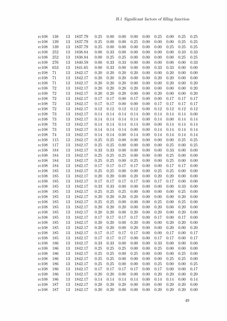
B.1 Significant factors of filling function
rc108 138 13 1837.79 0.25 0.00 0.00 0.00 0.00 0.25 0.00 0.25 0.25rc108 139 13 1837.79 0.25 0.00 0.00 0.25 0.00 0.00 0.00 0.25 0.25rc108 139 13 1837.79 0.25 0.00 0.00 0.00 0.00 0.00 0.25 0.25 0.25rc108 252 13 1838.84 0.00 0.33 0.00 0.00 0.00 0.00 0.00 0.33 0.33rc108 252 13 1838.84 0.00 0.25 0.25 0.00 0.00 0.00 0.00 0.25 0.25rc108 276 13 1840.59 0.00 0.33 0.33 0.00 0.00 0.00 0.00 0.00 0.33rc108 653 13 1841.65 0.00 0.33 0.00 0.00 0.00 0.33 0.33 0.00 0.00rc108 71 13 1842.17 0.20 0.20 0.20 0.20 0.00 0.00 0.20 0.00 0.00rc108 71 13 1842.17 0.20 0.20 0.20 0.00 0.00 0.20 0.20 0.00 0.00rc108 71 13 1842.17 0.20 0.20 0.20 0.00 0.00 0.00 0.20 0.00 0.20rc108 72 13 1842.17 0.20 0.20 0.20 0.20 0.00 0.00 0.00 0.00 0.20rc108 72 13 1842.17 0.20 0.20 0.20 0.00 0.00 0.20 0.00 0.00 0.20rc108 72 13 1842.17 0.17 0.17 0.00 0.17 0.00 0.00 0.17 0.17 0.17rc108 72 13 1842.17 0.17 0.17 0.00 0.00 0.00 0.17 0.17 0.17 0.17rc108 72 13 1842.17 0.12 0.12 0.12 0.12 0.00 0.12 0.12 0.12 0.12rc108 73 13 1842.17 0.14 0.14 0.14 0.14 0.00 0.14 0.14 0.14 0.00rc108 73 13 1842.17 0.14 0.14 0.14 0.14 0.00 0.14 0.00 0.14 0.14rc108 73 13 1842.17 0.14 0.14 0.14 0.14 0.00 0.00 0.14 0.14 0.14rc108 73 13 1842.17 0.14 0.14 0.14 0.00 0.00 0.14 0.14 0.14 0.14rc108 74 13 1842.17 0.14 0.14 0.00 0.14 0.00 0.14 0.14 0.14 0.14rc108 115 13 1842.17 0.25 0.25 0.00 0.00 0.00 0.00 0.00 0.25 0.25rc108 117 13 1842.17 0.25 0.25 0.00 0.00 0.00 0.00 0.25 0.00 0.25rc108 184 13 1842.17 0.33 0.33 0.00 0.00 0.00 0.00 0.33 0.00 0.00rc108 184 13 1842.17 0.25 0.25 0.25 0.00 0.00 0.00 0.25 0.00 0.00rc108 184 13 1842.17 0.25 0.25 0.00 0.25 0.00 0.00 0.25 0.00 0.00rc108 184 13 1842.17 0.17 0.17 0.17 0.17 0.00 0.00 0.17 0.17 0.00rc108 185 13 1842.17 0.25 0.25 0.00 0.00 0.00 0.25 0.25 0.00 0.00rc108 185 13 1842.17 0.20 0.20 0.00 0.20 0.00 0.20 0.20 0.00 0.00rc108 185 13 1842.17 0.17 0.17 0.17 0.17 0.00 0.17 0.17 0.00 0.00rc108 185 13 1842.17 0.33 0.33 0.00 0.00 0.00 0.00 0.00 0.33 0.00rc108 185 13 1842.17 0.25 0.25 0.25 0.00 0.00 0.00 0.00 0.25 0.00rc108 185 13 1842.17 0.20 0.20 0.20 0.20 0.00 0.00 0.00 0.20 0.00rc108 185 13 1842.17 0.25 0.25 0.00 0.00 0.00 0.25 0.00 0.25 0.00rc108 185 13 1842.17 0.20 0.20 0.20 0.00 0.00 0.20 0.00 0.20 0.00rc108 185 13 1842.17 0.20 0.20 0.00 0.20 0.00 0.20 0.00 0.20 0.00rc108 185 13 1842.17 0.17 0.17 0.17 0.17 0.00 0.17 0.00 0.17 0.00rc108 185 13 1842.17 0.20 0.20 0.00 0.20 0.00 0.00 0.20 0.20 0.00rc108 185 13 1842.17 0.20 0.20 0.00 0.20 0.00 0.00 0.20 0.00 0.20rc108 185 13 1842.17 0.17 0.17 0.17 0.17 0.00 0.00 0.17 0.00 0.17rc108 185 13 1842.17 0.17 0.17 0.17 0.00 0.00 0.17 0.17 0.00 0.17rc108 186 13 1842.17 0.33 0.33 0.00 0.00 0.00 0.33 0.00 0.00 0.00rc108 186 13 1842.17 0.25 0.25 0.25 0.00 0.00 0.25 0.00 0.00 0.00rc108 186 13 1842.17 0.25 0.25 0.00 0.25 0.00 0.00 0.00 0.25 0.00rc108 186 13 1842.17 0.25 0.25 0.00 0.00 0.00 0.00 0.25 0.25 0.00rc108 186 13 1842.17 0.25 0.25 0.00 0.00 0.00 0.25 0.00 0.00 0.25rc108 186 13 1842.17 0.17 0.17 0.17 0.17 0.00 0.17 0.00 0.00 0.17rc108 186 13 1842.17 0.20 0.20 0.00 0.00 0.00 0.20 0.20 0.00 0.20rc108 186 13 1842.17 0.14 0.14 0.14 0.14 0.00 0.14 0.14 0.00 0.14rc108 187 13 1842.17 0.20 0.20 0.20 0.00 0.00 0.00 0.20 0.20 0.00rc108 187 13 1842.17 0.20 0.20 0.00 0.00 0.00 0.20 0.20 0.20 0.00
49

B Data
rc108 187 13 1842.17 0.17 0.17 0.17 0.00 0.00 0.17 0.17 0.17 0.00rc108 187 13 1842.17 0.25 0.25 0.25 0.00 0.00 0.00 0.00 0.00 0.25rc108 187 13 1842.17 0.25 0.25 0.00 0.25 0.00 0.00 0.00 0.00 0.25rc108 187 13 1842.17 0.20 0.20 0.00 0.20 0.00 0.20 0.00 0.00 0.20rc108 187 13 1842.17 0.17 0.17 0.00 0.17 0.00 0.17 0.17 0.00 0.17rc108 187 13 1842.17 0.17 0.17 0.17 0.00 0.00 0.17 0.00 0.17 0.17rc108 187 13 1842.17 0.17 0.17 0.00 0.17 0.00 0.17 0.00 0.17 0.17rc108 188 13 1842.17 0.17 0.17 0.00 0.17 0.00 0.17 0.17 0.17 0.00rc108 188 13 1842.17 0.33 0.33 0.00 0.00 0.00 0.00 0.00 0.00 0.33rc108 188 13 1842.17 0.20 0.20 0.20 0.00 0.00 0.00 0.00 0.20 0.20rc108 188 13 1842.17 0.20 0.20 0.00 0.20 0.00 0.00 0.00 0.20 0.20rc108 188 13 1842.17 0.17 0.17 0.17 0.17 0.00 0.00 0.00 0.17 0.17rc108 188 13 1842.17 0.20 0.20 0.00 0.00 0.00 0.20 0.00 0.20 0.20rc108 188 13 1842.17 0.20 0.20 0.00 0.00 0.00 0.00 0.20 0.20 0.20rc108 188 13 1842.17 0.17 0.17 0.17 0.00 0.00 0.00 0.17 0.17 0.17rc108 189 13 1842.17 0.25 0.25 0.00 0.25 0.00 0.25 0.00 0.00 0.00rc108 189 13 1842.17 0.20 0.20 0.20 0.20 0.00 0.20 0.00 0.00 0.00rc108 198 13 1844.00 0.20 0.20 0.20 0.00 0.20 0.20 0.00 0.00 0.00rc108 199 13 1844.00 0.25 0.25 0.00 0.00 0.25 0.00 0.00 0.00 0.25rc108 199 13 1844.00 0.20 0.20 0.20 0.00 0.20 0.00 0.00 0.00 0.20rc108 201 13 1844.00 0.25 0.25 0.00 0.00 0.25 0.25 0.00 0.00 0.00rc108 748 13 1844.08 0.00 0.20 0.20 0.20 0.00 0.00 0.00 0.20 0.20rc108 849 13 1844.08 0.00 0.20 0.20 0.20 0.00 0.20 0.00 0.20 0.00rc108 482 13 1845.41 0.00 0.17 0.00 0.17 0.17 0.17 0.00 0.17 0.17rc108 482 13 1845.41 0.00 0.14 0.14 0.14 0.14 0.14 0.00 0.14 0.14rc108 199 13 1848.25 0.00 0.20 0.00 0.20 0.20 0.20 0.00 0.00 0.20rc108 206 13 1848.25 0.00 0.17 0.17 0.17 0.17 0.17 0.00 0.00 0.17rc108 128 13 1852.11 0.14 0.00 0.00 0.14 0.14 0.14 0.14 0.14 0.14rc108 129 13 1852.11 0.12 0.00 0.12 0.12 0.12 0.12 0.12 0.12 0.12rc108 179 13 1854.15 0.25 0.00 0.25 0.00 0.00 0.00 0.25 0.00 0.25rc108 180 13 1854.15 0.33 0.00 0.33 0.00 0.00 0.33 0.00 0.00 0.00rc108 180 13 1854.15 0.17 0.00 0.17 0.17 0.00 0.17 0.17 0.17 0.00rc108 180 13 1854.15 0.33 0.00 0.00 0.00 0.00 0.00 0.00 0.33 0.33rc108 180 13 1854.15 0.17 0.00 0.17 0.17 0.00 0.00 0.17 0.17 0.17rc108 181 13 1854.15 0.17 0.00 0.17 0.17 0.00 0.17 0.00 0.17 0.17rc108 182 13 1854.15 0.17 0.00 0.17 0.17 0.00 0.17 0.17 0.00 0.17rc108 182 13 1854.15 0.17 0.00 0.17 0.00 0.00 0.17 0.17 0.17 0.17rc108 774 14 1857.36 0.00 0.20 0.00 0.20 0.00 0.20 0.20 0.20 0.00rc108 777 14 1857.36 0.00 0.17 0.17 0.17 0.00 0.17 0.17 0.17 0.00rc108 778 14 1857.36 0.00 0.20 0.00 0.20 0.00 0.00 0.20 0.20 0.20rc108 779 14 1857.36 0.00 0.17 0.17 0.17 0.00 0.00 0.17 0.17 0.17rc108 991 14 1858.35 0.00 0.17 0.17 0.00 0.00 0.17 0.17 0.17 0.17rc108 534 13 1859.81 0.00 0.33 0.00 0.00 0.00 0.00 0.33 0.33 0.00rc108 534 13 1859.81 0.00 0.25 0.25 0.00 0.00 0.00 0.25 0.25 0.00rc108 617 13 1859.81 0.00 0.25 0.25 0.00 0.00 0.25 0.25 0.00 0.00rc108 665 13 1859.81 0.00 0.50 0.00 0.00 0.00 0.00 0.50 0.00 0.00rc108 1086 13 1859.81 0.00 0.33 0.33 0.00 0.00 0.00 0.33 0.00 0.00rc108 760 13 1859.97 0.00 0.20 0.00 0.00 0.20 0.20 0.20 0.00 0.20rc108 764 13 1859.97 0.00 0.17 0.17 0.00 0.17 0.17 0.17 0.00 0.17rc108 928 13 1859.97 0.00 0.14 0.14 0.00 0.14 0.14 0.14 0.14 0.14
50

B.1 Significant factors of filling function
rc108 929 13 1859.97 0.00 0.17 0.00 0.00 0.17 0.17 0.17 0.17 0.17rc108 317 13 1865.12 0.00 0.33 0.00 0.00 0.33 0.00 0.00 0.33 0.00rc108 317 13 1865.12 0.00 0.25 0.25 0.00 0.25 0.00 0.00 0.25 0.00rc108 278 13 1866.11 0.00 0.25 0.00 0.00 0.25 0.00 0.25 0.25 0.00rc108 279 13 1866.11 0.00 0.25 0.00 0.25 0.25 0.00 0.00 0.25 0.00rc108 279 13 1866.11 0.00 0.20 0.20 0.20 0.20 0.00 0.00 0.20 0.00rc108 282 13 1866.11 0.00 0.20 0.20 0.00 0.20 0.00 0.20 0.20 0.00rc108 957 14 1866.55 0.00 0.20 0.20 0.20 0.20 0.00 0.20 0.00 0.00rc108 958 14 1866.55 0.00 0.25 0.00 0.25 0.25 0.00 0.25 0.00 0.00rc108 292 13 1867.64 0.00 0.33 0.00 0.00 0.00 0.33 0.00 0.33 0.00rc108 292 13 1867.64 0.00 0.25 0.25 0.00 0.00 0.25 0.00 0.25 0.00rc108 295 13 1867.64 0.00 0.25 0.25 0.00 0.00 0.25 0.00 0.00 0.25rc108 122 13 1868.25 0.25 0.25 0.25 0.00 0.25 0.00 0.00 0.00 0.00rc108 123 13 1868.25 0.33 0.33 0.00 0.00 0.33 0.00 0.00 0.00 0.00rc108 483 13 1868.44 0.00 0.50 0.00 0.00 0.00 0.00 0.00 0.00 0.50rc108 165 13 1868.75 0.50 0.00 0.00 0.00 0.50 0.00 0.00 0.00 0.00rc108 167 13 1868.75 0.33 0.00 0.33 0.00 0.33 0.00 0.00 0.00 0.00rc108 191 13 1868.83 0.00 0.50 0.00 0.00 0.00 0.00 0.00 0.50 0.00rc108 191 13 1868.83 0.00 0.33 0.33 0.00 0.00 0.00 0.00 0.33 0.00rc108 113 14 1869.28 0.00 0.00 0.00 0.00 0.25 0.25 0.25 0.25 0.00rc108 113 14 1869.28 0.00 0.00 0.20 0.00 0.20 0.20 0.20 0.20 0.00rc108 132 13 1870.01 0.14 0.14 0.00 0.14 0.14 0.14 0.14 0.14 0.00rc108 132 13 1870.01 0.12 0.12 0.12 0.12 0.12 0.12 0.12 0.12 0.00rc108 132 13 1870.01 0.14 0.14 0.00 0.14 0.14 0.14 0.00 0.14 0.14rc108 132 13 1870.01 0.12 0.12 0.12 0.12 0.12 0.12 0.00 0.12 0.12rc108 132 13 1870.01 0.14 0.14 0.00 0.14 0.14 0.00 0.14 0.14 0.14rc108 132 13 1870.01 0.12 0.12 0.12 0.12 0.12 0.00 0.12 0.12 0.12rc108 132 13 1870.01 0.14 0.14 0.00 0.00 0.14 0.14 0.14 0.14 0.14rc108 132 13 1870.01 0.12 0.12 0.12 0.00 0.12 0.12 0.12 0.12 0.12rc108 145 13 1870.01 0.17 0.17 0.00 0.17 0.17 0.17 0.17 0.00 0.00rc108 145 13 1870.01 0.14 0.14 0.14 0.14 0.14 0.14 0.14 0.00 0.00rc108 146 13 1870.01 0.17 0.17 0.00 0.17 0.17 0.17 0.00 0.00 0.17rc108 146 13 1870.01 0.17 0.17 0.00 0.17 0.17 0.00 0.17 0.00 0.17rc108 146 13 1870.01 0.17 0.17 0.00 0.00 0.17 0.17 0.17 0.00 0.17rc108 147 13 1870.01 0.14 0.14 0.14 0.14 0.14 0.14 0.00 0.00 0.14rc108 147 13 1870.01 0.14 0.14 0.14 0.14 0.14 0.00 0.14 0.00 0.14rc108 147 13 1870.01 0.14 0.14 0.14 0.00 0.14 0.14 0.14 0.00 0.14rc108 178 13 1870.01 0.17 0.17 0.17 0.17 0.17 0.17 0.00 0.00 0.00rc108 179 13 1870.01 0.20 0.20 0.00 0.20 0.20 0.00 0.20 0.00 0.00rc108 179 13 1870.01 0.17 0.17 0.17 0.17 0.17 0.00 0.17 0.00 0.00rc108 179 13 1870.01 0.20 0.20 0.00 0.00 0.20 0.20 0.20 0.00 0.00rc108 179 13 1870.01 0.17 0.17 0.17 0.00 0.17 0.17 0.17 0.00 0.00rc108 179 13 1870.01 0.17 0.17 0.00 0.17 0.17 0.17 0.00 0.17 0.00rc108 179 13 1870.01 0.14 0.14 0.14 0.14 0.14 0.14 0.00 0.14 0.00rc108 179 13 1870.01 0.17 0.17 0.17 0.00 0.17 0.17 0.00 0.00 0.17rc108 179 13 1870.01 0.20 0.20 0.00 0.00 0.20 0.00 0.20 0.00 0.20rc108 179 13 1870.01 0.17 0.17 0.17 0.00 0.17 0.00 0.17 0.00 0.17rc108 180 13 1870.01 0.20 0.20 0.00 0.20 0.20 0.20 0.00 0.00 0.00rc108 180 13 1870.01 0.14 0.14 0.14 0.14 0.14 0.00 0.14 0.14 0.00rc108 180 13 1870.01 0.17 0.17 0.00 0.00 0.17 0.17 0.17 0.17 0.00
51

B Data
rc108 180 13 1870.01 0.20 0.20 0.00 0.20 0.20 0.00 0.00 0.00 0.20rc108 180 13 1870.01 0.17 0.17 0.17 0.17 0.17 0.00 0.00 0.00 0.17rc108 180 13 1870.01 0.20 0.20 0.00 0.00 0.20 0.20 0.00 0.00 0.20rc108 181 13 1870.01 0.17 0.17 0.00 0.17 0.17 0.00 0.17 0.17 0.00rc108 181 13 1870.01 0.14 0.14 0.14 0.00 0.14 0.14 0.14 0.14 0.00rc108 181 13 1870.01 0.14 0.14 0.14 0.14 0.14 0.00 0.00 0.14 0.14rc108 181 13 1870.01 0.17 0.17 0.00 0.00 0.17 0.17 0.00 0.17 0.17rc108 181 13 1870.01 0.14 0.14 0.14 0.00 0.14 0.14 0.00 0.14 0.14rc108 181 13 1870.01 0.17 0.17 0.00 0.00 0.17 0.00 0.17 0.17 0.17rc108 181 13 1870.01 0.14 0.14 0.14 0.00 0.14 0.00 0.14 0.14 0.14rc108 182 13 1870.01 0.17 0.17 0.00 0.17 0.17 0.00 0.00 0.17 0.17rc108 169 13 1870.51 0.20 0.20 0.20 0.20 0.20 0.00 0.00 0.00 0.00rc108 600 13 1871.22 0.00 0.17 0.00 0.17 0.17 0.17 0.17 0.00 0.17rc108 603 13 1871.22 0.00 0.14 0.14 0.14 0.14 0.14 0.14 0.00 0.14rc108 149 13 1871.98 0.00 0.50 0.00 0.00 0.50 0.00 0.00 0.00 0.00rc108 150 13 1871.98 0.00 0.33 0.33 0.00 0.33 0.00 0.00 0.00 0.00rc108 307 13 1873.39 0.00 0.33 0.00 0.00 0.33 0.00 0.00 0.00 0.33rc108 307 13 1873.39 0.00 0.25 0.25 0.00 0.25 0.00 0.00 0.00 0.25rc108 136 13 1873.59 0.33 0.33 0.33 0.00 0.00 0.00 0.00 0.00 0.00rc108 136 13 1873.59 0.25 0.25 0.25 0.25 0.00 0.00 0.00 0.00 0.00rc108 137 13 1873.59 0.50 0.50 0.00 0.00 0.00 0.00 0.00 0.00 0.00rc108 137 13 1873.59 0.33 0.33 0.00 0.33 0.00 0.00 0.00 0.00 0.00rc108 558 14 1874.66 0.00 0.14 0.14 0.14 0.14 0.14 0.14 0.14 0.00rc108 560 14 1874.66 0.00 0.17 0.00 0.17 0.17 0.17 0.17 0.17 0.00rc108 892 14 1874.66 0.00 0.12 0.12 0.12 0.12 0.12 0.12 0.12 0.12rc108 893 14 1874.66 0.00 0.14 0.00 0.14 0.14 0.14 0.14 0.14 0.14rc108 781 13 1876.62 0.00 0.20 0.20 0.00 0.00 0.20 0.20 0.00 0.20rc108 155 13 1877.17 0.20 0.00 0.00 0.20 0.20 0.00 0.20 0.00 0.20rc108 167 13 1877.17 0.17 0.00 0.17 0.17 0.17 0.00 0.17 0.00 0.17rc108 147 13 1877.63 0.25 0.00 0.25 0.25 0.25 0.00 0.00 0.00 0.00rc108 152 13 1877.63 0.25 0.00 0.25 0.25 0.25 0.00 0.00 0.00 0.00rc108 865 13 1877.99 0.00 0.20 0.00 0.20 0.20 0.00 0.20 0.00 0.20rc108 886 13 1877.99 0.00 0.17 0.17 0.17 0.17 0.00 0.17 0.00 0.17rc108 598 13 1881.51 0.00 0.25 0.25 0.00 0.25 0.25 0.00 0.00 0.00rc108 605 13 1881.51 0.00 0.33 0.00 0.00 0.33 0.33 0.00 0.00 0.00rc108 1181 13 1881.83 0.00 0.20 0.20 0.20 0.00 0.20 0.00 0.00 0.20rc108 924 14 1882.95 0.00 0.20 0.00 0.20 0.20 0.00 0.20 0.20 0.00rc108 924 14 1882.95 0.00 0.17 0.17 0.17 0.17 0.00 0.17 0.17 0.00rc108 1012 13 1883.76 0.00 0.17 0.17 0.17 0.00 0.17 0.17 0.00 0.17rc108 600 13 1883.8 0.00 0.17 0.00 0.17 0.00 0.17 0.17 0.17 0.17rc108 600 13 1883.8 0.00 0.14 0.14 0.14 0.00 0.14 0.14 0.14 0.14rc108 141 13 1884.77 0.17 0.00 0.00 0.17 0.17 0.00 0.17 0.17 0.17rc108 141 13 1884.77 0.14 0.00 0.14 0.14 0.14 0.00 0.14 0.14 0.14rc108 326 13 1885.89 0.00 0.20 0.00 0.00 0.20 0.00 0.20 0.20 0.20rc108 326 13 1885.89 0.00 0.17 0.17 0.00 0.17 0.00 0.17 0.17 0.17rc108 403 13 1886.97 0.20 0.20 0.00 0.00 0.20 0.20 0.00 0.20 0.00rc108 403 13 1886.97 0.17 0.17 0.17 0.00 0.17 0.17 0.00 0.17 0.00rc108 404 13 1886.97 0.20 0.20 0.00 0.20 0.20 0.00 0.00 0.20 0.00rc108 404 13 1886.97 0.17 0.17 0.17 0.17 0.17 0.00 0.00 0.17 0.00rc108 407 13 1886.97 0.17 0.17 0.17 0.00 0.17 0.00 0.17 0.17 0.00
52

B.1 Significant factors of filling function
rc108 409 13 1886.97 0.20 0.20 0.00 0.00 0.20 0.00 0.20 0.20 0.00rc108 409 13 1886.97 0.20 0.20 0.00 0.00 0.20 0.00 0.00 0.20 0.20rc108 409 13 1886.97 0.17 0.17 0.17 0.00 0.17 0.00 0.00 0.17 0.17rc108 332 13 1889.31 0.17 0.00 0.00 0.17 0.17 0.17 0.00 0.17 0.17rc108 332 13 1889.31 0.14 0.00 0.14 0.14 0.14 0.14 0.00 0.14 0.14rc108 156 13 1889.91 0.00 0.25 0.00 0.25 0.25 0.25 0.00 0.00 0.00rc108 156 13 1889.91 0.00 0.25 0.00 0.00 0.25 0.25 0.25 0.00 0.00rc108 156 13 1889.91 0.00 0.20 0.20 0.00 0.20 0.20 0.20 0.00 0.00rc108 156 13 1889.91 0.00 0.25 0.00 0.00 0.25 0.00 0.25 0.00 0.25rc108 156 13 1889.91 0.00 0.20 0.20 0.00 0.20 0.00 0.20 0.00 0.20rc108 157 13 1889.91 0.00 0.25 0.00 0.25 0.25 0.00 0.00 0.00 0.25rc108 157 13 1889.91 0.00 0.20 0.20 0.20 0.20 0.00 0.00 0.00 0.20rc108 158 13 1889.91 0.00 0.20 0.20 0.20 0.20 0.20 0.00 0.00 0.00rc108 283 13 1889.91 0.00 0.20 0.20 0.00 0.20 0.20 0.00 0.00 0.20rc108 285 13 1889.91 0.00 0.25 0.00 0.00 0.25 0.25 0.00 0.00 0.25rc108 581 13 1889.91 0.00 0.20 0.00 0.20 0.20 0.20 0.00 0.20 0.00rc108 581 13 1889.91 0.00 0.17 0.17 0.17 0.17 0.17 0.00 0.17 0.00rc108 586 13 1889.91 0.00 0.17 0.17 0.00 0.17 0.17 0.17 0.17 0.00rc108 587 13 1889.91 0.00 0.20 0.00 0.00 0.20 0.20 0.20 0.20 0.00rc108 588 13 1889.91 0.00 0.20 0.00 0.20 0.20 0.00 0.00 0.20 0.20rc108 589 13 1889.91 0.00 0.17 0.17 0.17 0.17 0.00 0.00 0.17 0.17rc108 105 14 1891.09 0.00 0.00 0.00 0.00 0.50 0.00 0.50 0.00 0.00rc108 207 14 1891.09 0.00 0.00 0.33 0.00 0.33 0.00 0.33 0.00 0.00rc108 228 13 1891.27 0.00 0.50 0.00 0.00 0.00 0.50 0.00 0.00 0.00rc108 416 13 1892.19 0.00 0.33 0.00 0.00 0.33 0.00 0.33 0.00 0.00rc108 417 13 1892.19 0.00 0.25 0.25 0.00 0.25 0.00 0.25 0.00 0.00rc108 248 13 1892.75 0.00 0.50 0.00 0.50 0.00 0.00 0.00 0.00 0.00rc108 244 13 1896.74 0.00 1.00 0.00 0.00 0.00 0.00 0.00 0.00 0.00rc108 372 13 1896.74 0.00 0.50 0.50 0.00 0.00 0.00 0.00 0.00 0.00rc108 121 13 1898.72 0.17 0.00 0.17 0.17 0.17 0.17 0.17 0.00 0.00rc108 122 13 1898.72 0.20 0.00 0.00 0.20 0.20 0.20 0.20 0.00 0.00rc108 123 13 1898.72 0.17 0.00 0.00 0.17 0.17 0.17 0.17 0.17 0.00rc108 123 13 1898.72 0.14 0.00 0.14 0.14 0.14 0.14 0.14 0.14 0.00rc108 459 13 1900.07 0.00 0.20 0.20 0.20 0.00 0.20 0.20 0.00 0.00rc108 265 13 1900.19 0.00 0.33 0.33 0.00 0.00 0.33 0.00 0.00 0.00rc108 601 13 1903.00 0.00 0.25 0.00 0.00 0.00 0.25 0.25 0.25 0.00rc108 601 13 1903.00 0.00 0.20 0.20 0.00 0.00 0.20 0.20 0.20 0.00rc108 603 13 1903.00 0.00 0.20 0.00 0.00 0.00 0.20 0.20 0.20 0.20rc108 141 13 1904.22 0.00 0.25 0.00 0.00 0.25 0.00 0.00 0.25 0.25rc108 142 13 1904.22 0.00 0.20 0.20 0.00 0.20 0.00 0.00 0.20 0.20rc108 742 14 1905.15 0.00 0.25 0.00 0.25 0.00 0.25 0.25 0.00 0.00rc108 877 13 1907.66 0.00 0.17 0.17 0.17 0.17 0.17 0.17 0.00 0.00rc108 880 13 1907.66 0.00 0.20 0.00 0.20 0.20 0.20 0.20 0.00 0.00rc108 624 13 1908.79 0.00 0.25 0.00 0.25 0.00 0.25 0.00 0.00 0.25rc108 107 13 1912.37 0.20 0.00 0.00 0.20 0.20 0.20 0.00 0.20 0.00rc108 107 13 1912.37 0.17 0.00 0.17 0.17 0.17 0.17 0.00 0.17 0.00rc108 107 13 1912.37 0.20 0.00 0.00 0.00 0.20 0.20 0.20 0.20 0.00rc108 108 13 1912.37 0.20 0.00 0.00 0.20 0.20 0.00 0.20 0.20 0.00rc108 108 13 1912.37 0.17 0.00 0.17 0.17 0.17 0.00 0.17 0.17 0.00rc108 108 13 1912.37 0.17 0.00 0.17 0.00 0.17 0.17 0.17 0.17 0.00
53

B Data
rc108 108 13 1912.37 0.20 0.00 0.00 0.20 0.20 0.00 0.00 0.20 0.20rc108 108 13 1912.37 0.17 0.00 0.17 0.17 0.17 0.00 0.00 0.17 0.17rc108 108 13 1912.37 0.17 0.00 0.17 0.00 0.17 0.00 0.17 0.17 0.17rc108 109 13 1912.37 0.20 0.00 0.00 0.00 0.20 0.00 0.20 0.20 0.20rc108 113 14 1912.73 0.00 0.00 0.00 0.00 0.50 0.00 0.00 0.50 0.00rc108 521 13 1913.23 0.00 0.20 0.00 0.20 0.00 0.20 0.00 0.20 0.20rc108 1085 13 1913.23 0.00 0.17 0.17 0.17 0.00 0.17 0.00 0.17 0.17rc108 1211 13 1913.23 0.00 0.25 0.00 0.25 0.00 0.00 0.00 0.25 0.25rc108 1268 13 1913.23 0.00 0.25 0.00 0.25 0.00 0.25 0.00 0.25 0.00rc108 112 13 1913.72 0.14 0.14 0.00 0.14 0.14 0.14 0.14 0.00 0.14rc108 112 13 1913.72 0.12 0.12 0.12 0.12 0.12 0.12 0.12 0.00 0.12rc108 112 13 1913.72 0.12 0.12 0.00 0.12 0.12 0.12 0.12 0.12 0.12rc108 112 13 1913.72 0.11 0.11 0.11 0.11 0.11 0.11 0.11 0.11 0.11rc108 810 14 1913.95 0.00 0.25 0.00 0.00 0.00 0.25 0.25 0.00 0.25rc108 110 13 1917.52 0.25 0.00 0.00 0.25 0.25 0.00 0.25 0.00 0.00rc108 110 13 1917.52 0.25 0.00 0.00 0.00 0.25 0.00 0.25 0.00 0.25rc108 111 13 1917.52 0.25 0.00 0.00 0.25 0.25 0.25 0.00 0.00 0.00rc108 111 13 1917.52 0.20 0.00 0.20 0.20 0.20 0.00 0.20 0.00 0.00rc108 111 13 1917.52 0.25 0.00 0.00 0.00 0.25 0.25 0.25 0.00 0.00rc108 111 13 1917.52 0.20 0.00 0.20 0.00 0.20 0.20 0.20 0.00 0.00rc108 111 13 1917.52 0.25 0.00 0.00 0.25 0.25 0.00 0.00 0.00 0.25rc108 111 13 1917.52 0.25 0.00 0.00 0.00 0.25 0.25 0.00 0.00 0.25rc108 111 13 1917.52 0.20 0.00 0.20 0.00 0.20 0.20 0.00 0.00 0.20rc108 111 13 1917.52 0.20 0.00 0.20 0.00 0.20 0.00 0.20 0.00 0.20rc108 112 13 1917.52 0.20 0.00 0.20 0.20 0.20 0.20 0.00 0.00 0.00rc108 112 13 1917.52 0.20 0.00 0.20 0.20 0.20 0.00 0.00 0.00 0.20rc108 137 13 1917.52 0.17 0.00 0.00 0.00 0.17 0.17 0.17 0.17 0.17rc108 137 13 1917.52 0.14 0.00 0.14 0.00 0.14 0.14 0.14 0.14 0.14rc108 143 13 1917.52 0.20 0.00 0.00 0.00 0.20 0.20 0.00 0.20 0.20rc108 143 13 1917.52 0.17 0.00 0.17 0.00 0.17 0.17 0.00 0.17 0.17rc108 285 13 1917.52 0.14 0.00 0.14 0.14 0.14 0.14 0.14 0.00 0.14rc108 287 13 1917.52 0.17 0.00 0.00 0.17 0.17 0.17 0.17 0.00 0.17rc108 96 13 1918.07 0.33 0.00 0.00 0.00 0.33 0.00 0.00 0.33 0.00rc108 96 13 1918.07 0.25 0.00 0.25 0.00 0.25 0.00 0.00 0.25 0.00rc108 103 13 1918.07 0.25 0.00 0.00 0.00 0.25 0.00 0.25 0.25 0.00rc108 104 13 1918.07 0.25 0.00 0.00 0.25 0.25 0.00 0.00 0.25 0.00rc108 104 13 1918.07 0.20 0.00 0.20 0.20 0.20 0.00 0.00 0.20 0.00rc108 104 13 1918.07 0.25 0.00 0.00 0.00 0.25 0.25 0.00 0.25 0.00rc108 104 13 1918.07 0.20 0.00 0.20 0.00 0.20 0.20 0.00 0.20 0.00rc108 105 13 1918.07 0.20 0.00 0.20 0.00 0.20 0.00 0.20 0.20 0.00rc108 105 13 1918.07 0.25 0.00 0.00 0.00 0.25 0.00 0.00 0.25 0.25rc108 105 13 1918.07 0.20 0.00 0.20 0.00 0.20 0.00 0.00 0.20 0.20rc108 118 13 1919.26 0.25 0.25 0.00 0.00 0.25 0.00 0.00 0.25 0.00rc108 118 13 1919.26 0.20 0.20 0.20 0.00 0.20 0.00 0.00 0.20 0.00rc108 706 13 1920.10 0.00 0.17 0.00 0.17 0.17 0.00 0.17 0.17 0.17rc108 707 13 1920.10 0.00 0.14 0.14 0.14 0.14 0.00 0.14 0.14 0.14rc108 141 14 1920.50 0.00 0.00 0.00 0.00 0.33 0.00 0.33 0.33 0.00rc108 143 14 1920.50 0.00 0.00 0.25 0.00 0.25 0.00 0.25 0.25 0.00rc108 500 13 1920.52 0.00 0.25 0.25 0.25 0.00 0.00 0.25 0.00 0.00rc108 540 13 1920.52 0.00 0.33 0.00 0.00 0.00 0.00 0.33 0.00 0.33
54

B.1 Significant factors of filling function
rc108 541 13 1920.52 0.00 0.25 0.25 0.00 0.00 0.00 0.25 0.00 0.25rc108 591 13 1920.52 0.00 0.33 0.00 0.33 0.00 0.00 0.00 0.00 0.33rc108 647 13 1920.52 0.00 0.33 0.00 0.33 0.00 0.00 0.00 0.33 0.00rc108 647 13 1920.52 0.00 0.25 0.25 0.25 0.00 0.00 0.00 0.25 0.00rc108 709 13 1920.52 0.00 0.20 0.20 0.20 0.00 0.00 0.20 0.00 0.20rc108 731 13 1920.52 0.00 0.20 0.20 0.20 0.00 0.00 0.20 0.20 0.00rc108 732 13 1920.52 0.00 0.33 0.00 0.33 0.00 0.00 0.33 0.00 0.00rc108 736 13 1920.52 0.00 0.25 0.00 0.25 0.00 0.00 0.25 0.25 0.00rc108 1004 13 1920.52 0.00 0.25 0.00 0.25 0.00 0.00 0.25 0.00 0.25rc108 556 13 1923.98 0.00 0.33 0.00 0.00 0.00 0.33 0.00 0.00 0.33rc108 247 14 1924.99 0.00 0.00 0.00 0.00 0.50 0.00 0.00 0.00 0.50rc108 248 14 1924.99 0.00 0.00 0.33 0.00 0.33 0.00 0.00 0.00 0.33rc108 189 14 1925.64 0.00 0.00 0.25 0.00 0.25 0.25 0.00 0.25 0.00rc108 817 13 1926.75 0.00 0.20 0.20 0.00 0.00 0.20 0.00 0.20 0.20rc108 818 13 1926.75 0.00 0.25 0.00 0.00 0.00 0.25 0.00 0.25 0.25rc108 134 14 1935.59 0.00 0.00 0.33 0.33 0.33 0.00 0.00 0.00 0.00rc108 138 13 1936.82 0.00 0.25 0.00 0.00 0.25 0.25 0.00 0.25 0.00rc108 138 13 1936.82 0.00 0.20 0.20 0.00 0.20 0.20 0.00 0.20 0.00rc108 880 13 1936.82 0.00 0.25 0.25 0.25 0.25 0.00 0.00 0.00 0.00rc108 189 14 1947.98 0.00 0.00 0.00 0.00 0.33 0.33 0.00 0.33 0.00rc108 85 14 1954.16 0.00 0.00 0.00 0.00 0.00 0.50 0.00 0.00 0.50rc108 64 14 1957.65 0.00 0.00 0.33 0.00 0.00 0.33 0.00 0.33 0.00rc108 69 14 1957.65 0.00 0.00 0.33 0.00 0.00 0.33 0.00 0.00 0.33rc108 91 14 1957.65 0.00 0.00 0.00 0.00 0.00 0.50 0.00 0.50 0.00rc108 182 14 1965.05 0.00 0.00 0.00 0.00 0.25 0.25 0.00 0.25 0.25rc108 182 14 1965.05 0.00 0.00 0.20 0.00 0.20 0.20 0.00 0.20 0.20rc108 174 14 1977.35 0.00 0.00 0.00 0.50 0.50 0.00 0.00 0.00 0.00rc108 116 14 1978.29 0.00 0.00 0.00 0.00 0.20 0.20 0.20 0.20 0.20rc108 107 15 1986.20 0.00 0.00 0.17 0.17 0.17 0.17 0.00 0.17 0.17rc108 145 14 1991.67 0.00 0.00 0.00 0.20 0.20 0.20 0.00 0.20 0.20rc108 107 14 1995.62 0.00 0.00 0.00 0.25 0.25 0.00 0.00 0.25 0.25rc108 107 14 1995.62 0.00 0.00 0.20 0.20 0.20 0.00 0.00 0.20 0.20rc108 88 14 1997.71 0.00 0.00 0.17 0.00 0.17 0.17 0.17 0.17 0.17rc108 400 14 1998.94 0.00 0.00 0.00 0.00 0.33 0.33 0.00 0.00 0.33rc108 65 14 1999.26 0.00 0.00 0.00 0.33 0.33 0.33 0.00 0.00 0.00rc108 65 14 1999.26 0.00 0.00 0.25 0.25 0.25 0.25 0.00 0.00 0.00rc108 84 14 1999.26 0.00 0.00 0.00 0.25 0.25 0.25 0.00 0.25 0.00rc108 84 14 1999.26 0.00 0.00 0.20 0.20 0.20 0.20 0.00 0.20 0.00rc108 99 14 1999.26 0.00 0.00 0.00 0.00 0.33 0.33 0.33 0.00 0.00rc108 100 14 1999.26 0.00 0.00 0.25 0.00 0.25 0.25 0.25 0.00 0.00rc108 101 14 1999.26 0.00 0.00 0.00 0.20 0.20 0.20 0.20 0.20 0.00rc108 102 14 1999.26 0.00 0.00 0.17 0.17 0.17 0.17 0.17 0.17 0.00rc108 179 15 2000.58 0.00 0.00 0.00 0.00 1.00 0.00 0.00 0.00 0.00rc108 183 15 2000.58 0.00 0.00 0.50 0.00 0.50 0.00 0.00 0.00 0.00rc108 135 14 2005.52 0.00 0.00 0.00 0.00 0.50 0.50 0.00 0.00 0.00rc108 136 14 2005.52 0.00 0.00 0.33 0.00 0.33 0.33 0.00 0.00 0.00rc108 64 14 2006.10 0.00 0.00 0.00 0.00 0.00 0.00 0.00 0.00 1.00rc108 116 14 2006.75 0.00 0.00 0.00 0.00 0.25 0.00 0.25 0.25 0.25rc108 155 15 2011.15 0.00 0.00 0.25 0.00 0.25 0.25 0.00 0.00 0.25rc108 113 14 2043.96 0.00 0.00 0.00 0.00 0.33 0.00 0.00 0.33 0.33
55

B Data
rc108 114 14 2043.96 0.00 0.00 0.25 0.00 0.25 0.00 0.00 0.25 0.25rc108 86 15 2052.47 0.00 0.00 0.00 0.25 0.25 0.25 0.00 0.00 0.25rc108 144 15 2052.47 0.00 0.00 0.20 0.20 0.20 0.20 0.00 0.00 0.20rc108 198 15 2052.47 0.00 0.00 0.20 0.00 0.20 0.20 0.20 0.00 0.20rc108 199 15 2052.47 0.00 0.00 0.00 0.00 0.25 0.25 0.25 0.00 0.25rc108 34 15 2054.75 0.00 0.00 0.00 0.50 0.00 0.00 0.00 0.00 0.50rc108 44 15 2054.75 0.00 0.00 0.00 0.33 0.00 0.00 0.33 0.00 0.33rc108 48 15 2054.75 0.00 0.00 0.00 0.25 0.00 0.00 0.25 0.25 0.25rc108 48 15 2054.75 0.00 0.00 0.20 0.20 0.00 0.00 0.20 0.20 0.20rc108 49 15 2054.75 0.00 0.00 0.25 0.25 0.00 0.00 0.25 0.00 0.25rc108 51 15 2054.75 0.00 0.00 0.33 0.33 0.00 0.00 0.00 0.00 0.33rc108 49 15 2059.23 0.00 0.00 0.00 0.50 0.00 0.00 0.00 0.50 0.00rc108 58 15 2059.23 0.00 0.00 0.33 0.33 0.00 0.00 0.00 0.33 0.00rc108 44 15 2059.74 0.00 0.00 0.20 0.20 0.00 0.20 0.20 0.00 0.20rc108 45 15 2059.74 0.00 0.00 0.00 0.25 0.00 0.25 0.25 0.00 0.25rc108 50 15 2059.74 0.00 0.00 0.00 0.20 0.00 0.20 0.20 0.20 0.20rc108 50 15 2059.74 0.00 0.00 0.17 0.17 0.00 0.17 0.17 0.17 0.17rc108 54 15 2059.74 0.00 0.00 0.00 0.33 0.00 0.33 0.00 0.00 0.33rc108 54 15 2059.74 0.00 0.00 0.25 0.25 0.00 0.25 0.00 0.00 0.25rc108 46 15 2061.28 0.00 0.00 0.33 0.00 0.00 0.33 0.33 0.00 0.00rc108 50 15 2061.28 0.00 0.00 0.00 0.00 0.00 0.50 0.50 0.00 0.00rc108 64 15 2061.28 0.00 0.00 0.00 0.00 0.00 1.00 0.00 0.00 0.00rc108 68 15 2061.28 0.00 0.00 0.50 0.00 0.00 0.50 0.00 0.00 0.00rc108 157 15 2063.98 0.00 0.00 0.20 0.00 0.20 0.00 0.20 0.20 0.20rc108 219 14 2064.29 0.00 0.00 0.00 0.33 0.33 0.00 0.00 0.00 0.33rc108 219 14 2064.29 0.00 0.00 0.25 0.25 0.25 0.00 0.00 0.00 0.25rc108 42 15 2064.48 0.00 0.00 1.00 0.00 0.00 0.00 0.00 0.00 0.00rc108 45 15 2066.18 0.00 0.00 0.00 0.33 0.00 0.33 0.33 0.00 0.00rc108 48 15 2066.18 0.00 0.00 0.00 0.25 0.00 0.25 0.25 0.25 0.00rc108 49 15 2066.18 0.00 0.00 0.25 0.25 0.00 0.25 0.25 0.00 0.00rc108 65 15 2066.18 0.00 0.00 0.20 0.20 0.00 0.20 0.20 0.20 0.00rc108 40 15 2067.44 0.00 0.00 0.00 1.00 0.00 0.00 0.00 0.00 0.00rc108 41 15 2067.44 0.00 0.00 0.33 0.33 0.00 0.00 0.33 0.00 0.00rc108 42 15 2067.44 0.00 0.00 0.50 0.00 0.00 0.00 0.50 0.00 0.00rc108 44 15 2067.44 0.00 0.00 0.00 0.50 0.00 0.00 0.50 0.00 0.00rc108 47 15 2067.44 0.00 0.00 0.00 0.00 0.00 0.00 1.00 0.00 0.00rc108 48 15 2067.44 0.00 0.00 0.00 0.33 0.33 0.00 0.33 0.00 0.00rc108 49 15 2067.44 0.00 0.00 0.00 0.33 0.00 0.00 0.33 0.33 0.00rc108 49 15 2067.44 0.00 0.00 0.25 0.25 0.00 0.00 0.25 0.25 0.00rc108 63 15 2067.44 0.00 0.00 0.25 0.25 0.25 0.00 0.25 0.00 0.00rc108 67 15 2067.44 0.00 0.00 0.50 0.50 0.00 0.00 0.00 0.00 0.00rc108 68 15 2067.44 0.00 0.00 0.00 0.25 0.25 0.00 0.25 0.25 0.00rc108 68 15 2067.44 0.00 0.00 0.20 0.20 0.20 0.00 0.20 0.20 0.00rc108 93 15 2067.44 0.00 0.00 0.00 0.33 0.33 0.00 0.00 0.33 0.00rc108 93 15 2067.44 0.00 0.00 0.25 0.25 0.25 0.00 0.00 0.25 0.00rc108 43 15 2071.37 0.00 0.00 0.00 0.00 0.00 0.25 0.25 0.25 0.25rc108 44 15 2071.37 0.00 0.00 0.20 0.00 0.00 0.20 0.20 0.20 0.20rc108 53 15 2071.37 0.00 0.00 0.00 0.00 0.00 0.33 0.33 0.00 0.33rc108 53 15 2071.37 0.00 0.00 0.25 0.00 0.00 0.25 0.25 0.00 0.25rc108 54 15 2071.37 0.00 0.00 0.00 0.25 0.00 0.25 0.00 0.25 0.25
56

B.2 Tuning of search algorithm
rc108 54 15 2071.37 0.00 0.00 0.20 0.20 0.00 0.20 0.00 0.20 0.20rc108 43 15 2076.10 0.00 0.00 0.25 0.00 0.00 0.25 0.25 0.25 0.00rc108 44 15 2076.10 0.00 0.00 0.00 0.00 0.00 0.00 0.50 0.00 0.50rc108 45 15 2076.10 0.00 0.00 0.33 0.00 0.00 0.00 0.33 0.00 0.33rc108 46 15 2076.10 0.00 0.00 0.00 0.00 0.00 0.33 0.33 0.33 0.00rc108 47 15 2076.10 0.00 0.00 0.00 0.00 0.00 0.00 0.50 0.50 0.00rc108 47 15 2076.10 0.00 0.00 0.33 0.00 0.00 0.00 0.33 0.33 0.00rc108 52 15 2076.10 0.00 0.00 0.00 0.33 0.00 0.33 0.00 0.33 0.00rc108 52 15 2076.10 0.00 0.00 0.25 0.25 0.00 0.25 0.00 0.25 0.00rc108 62 15 2076.10 0.00 0.00 0.20 0.20 0.20 0.00 0.20 0.00 0.20rc108 62 15 2076.10 0.00 0.00 0.00 0.33 0.00 0.00 0.00 0.33 0.33rc108 63 15 2076.10 0.00 0.00 0.25 0.25 0.00 0.00 0.00 0.25 0.25rc108 73 15 2076.10 0.00 0.00 0.25 0.00 0.00 0.00 0.25 0.25 0.25rc108 74 15 2076.10 0.00 0.00 0.00 0.00 0.00 0.00 0.33 0.33 0.33rc108 75 15 2076.10 0.00 0.00 0.50 0.00 0.00 0.00 0.00 0.00 0.50rc108 77 15 2076.10 0.00 0.00 0.00 0.00 0.00 0.00 0.00 0.50 0.50rc108 77 15 2076.10 0.00 0.00 0.33 0.00 0.00 0.00 0.00 0.33 0.33rc108 77 15 2076.10 0.00 0.00 0.00 0.00 0.00 0.33 0.00 0.33 0.33rc108 77 15 2076.10 0.00 0.00 0.25 0.00 0.00 0.25 0.00 0.25 0.25rc108 78 15 2076.10 0.00 0.00 0.00 0.17 0.17 0.17 0.17 0.17 0.17rc108 78 15 2076.10 0.00 0.00 0.14 0.14 0.14 0.14 0.14 0.14 0.14rc108 81 15 2076.10 0.00 0.00 0.00 0.00 0.00 0.00 0.00 1.00 0.00rc108 86 15 2076.10 0.00 0.00 0.00 0.20 0.20 0.20 0.20 0.00 0.20rc108 86 15 2076.10 0.00 0.00 0.17 0.17 0.17 0.17 0.17 0.00 0.17rc108 92 15 2076.10 0.00 0.00 0.17 0.17 0.17 0.00 0.17 0.17 0.17rc108 93 15 2076.10 0.00 0.00 0.50 0.00 0.00 0.00 0.00 0.50 0.00rc108 96 15 2076.10 0.00 0.00 0.00 0.25 0.25 0.00 0.25 0.00 0.25rc108 97 15 2076.10 0.00 0.00 0.00 0.00 0.33 0.00 0.33 0.00 0.33rc108 97 15 2076.10 0.00 0.00 0.25 0.00 0.25 0.00 0.25 0.00 0.25rc108 99 15 2076.10 0.00 0.00 0.00 0.20 0.20 0.00 0.20 0.20 0.20rc108 127 15 2076.10 0.00 0.00 0.20 0.20 0.20 0.20 0.20 0.00 0.00rc108 137 15 2076.10 0.00 0.00 0.00 0.25 0.25 0.25 0.25 0.00 0.00rc108 45 14 2081.22 0.00 0.00 0.00 0.50 0.00 0.50 0.00 0.00 0.00rc108 53 14 2081.22 0.00 0.00 0.33 0.33 0.00 0.33 0.00 0.00 0.00rc108 124 14 2137.25 0.00 0.00 0.33 0.00 0.33 0.00 0.00 0.33 0.00
Table B.1: Running through the algorithm on data set rc108 with 0 or 1 as value for eachfactor of the filling function. This is done in order to determine, which factorsare the most significant. The data is sorted by total distance and plotted inFigure 5.1.
B.2 Tuning of search algorithm
CPU V Distance l_max k_max d_maxrc108 279.0 13 1841.6390794978788 6 3 1rc108 136.0 13 1818.9724744449716 6 3 3rc108 98.0 13 1905.007934696568 6 3 6
57

B Data
rc108 592.0 13 1805.3526045786984 6 4 1rc108 530.0 13 1777.1104033062443 6 4 3rc108 190.0 13 1893.6253780370464 6 4 6rc108 987.0 13 1818.9476179847238 6 5 1rc108 425.0 13 1860.249250330895 6 5 3rc108 286.0 13 1866.2375815568384 6 5 6rc108 506.0 13 1826.6503026078647 9 3 1rc108 252.0 13 1818.9724744449716 9 3 3rc108 134.0 13 1905.007934696568 9 3 6rc108 1065.0 13 1800.6436324695246 9 4 1rc108 647.0 13 1777.1104033062443 9 4 3rc108 426.0 13 1839.7307320121433 9 4 6rc108 1269.0 13 1818.9476179847238 9 5 1rc108 662.0 13 1792.1648924315464 9 5 3rc108 675.0 13 1838.8131937440876 9 5 6rc108 710.0 13 1826.6503026078647 12 3 1rc108 328.0 13 1818.9724744449716 12 3 3rc108 148.0 13 1893.6867037717745 12 3 6rc108 1330.0 13 1800.6436324695246 12 4 1rc108 806.0 13 1777.1104033062443 12 4 3rc108 493.0 13 1839.7307320121433 12 4 6rc108 1831.0 13 1818.9476179847238 12 5 1rc108 1233.0 13 1792.1648924315464 12 5 3rc108 864.0 13 1838.8131937440876 12 5 6r112 445.0 12 1556.593100448906 6 3 1r112 197.0 12 1559.2476700978907 6 3 3r112 192.0 12 1537.174526635105 6 3 6r112 1039.0 12 1563.86073958881 6 4 1r112 428.0 12 1571.908161149551 6 4 3r112 234.0 12 1573.5685988560954 6 4 6r112 885.0 12 1576.4721993104056 6 5 1r112 964.0 12 1543.2260351367102 6 5 3r112 443.0 12 1543.2260351367102 6 5 6r112 648.0 12 1556.593100448906 9 3 1r112 420.0 12 1559.2476700978907 9 3 3r112 253.0 12 1537.174526635105 9 3 6r112 1233.0 12 1563.86073958881 9 4 1r112 833.0 12 1571.908161149551 9 4 3r112 346.0 12 1536.5045708291686 9 4 6r112 1412.0 12 1543.433344907333 9 5 1r112 1334.0 12 1543.2260351367102 9 5 3r112 637.0 12 1516.671917121077 9 5 6r112 868.0 12 1556.593100448906 12 3 1r112 461.0 12 1558.4968779992282 12 3 3r112 286.0 12 1537.174526635105 12 3 6r112 1526.0 12 1563.86073958881 12 4 1r112 1051.0 12 1569.3212320166958 12 4 3r112 411.0 12 1536.5045708291686 12 4 6r112 1930.0 12 1543.433344907333 12 5 1r112 2255.0 12 1543.2260351367102 12 5 3
58

B.2 Tuning of search algorithm
r112 765.0 12 1516.671917121077 12 5 6r211 152.0 4 1959.2127537206743 6 3 1r211 186.0 4 1985.0125943589278 6 3 3r211 143.0 4 1985.0125943589278 6 3 6r211 152.0 4 1959.2127537206743 6 4 1r211 186.0 4 1985.0125943589278 6 4 3r211 141.0 4 1985.0125943589278 6 4 6r211 149.0 4 1959.2127537206743 6 5 1r211 184.0 4 1985.0125943589278 6 5 3r211 140.0 4 1985.0125943589278 6 5 6r211 229.0 4 1959.2127537206743 9 3 1r211 247.0 4 1985.0125943589278 9 3 3r211 207.0 4 1985.0125943589278 9 3 6r211 228.0 4 1959.2127537206743 9 4 1r211 230.0 4 1985.0125943589278 9 4 3r211 205.0 4 1985.0125943589278 9 4 6r211 229.0 4 1959.2127537206743 9 5 1r211 228.0 4 1985.0125943589278 9 5 3r211 205.0 4 1985.0125943589278 9 5 6r211 311.0 4 1959.2127537206743 12 3 1r211 326.0 4 1847.4617030220193 12 3 3r211 284.0 4 1889.189651189795 12 3 6r211 312.0 4 1959.2127537206743 12 4 1r211 334.0 4 1985.0125943589278 12 4 3r211 285.0 4 1889.189651189795 12 4 6r211 310.0 4 1959.2127537206743 12 5 1r211 333.0 4 1985.0125943589278 12 5 3r211 285.0 4 1889.189651189795 12 5 6r101 1105.0 19 2007.3307072613225 6 3 1r101 851.0 19 1972.306355902318 6 3 3r101 376.0 19 1965.077508078404 6 3 6r101 2400.0 19 2032.4341972360965 6 4 1r101 2245.0 19 1944.9441406045821 6 4 3r101 739.0 19 1944.9441406045821 6 4 6r101 2413.0 19 2032.4341972360965 6 5 1r101 2431.0 19 1972.679292748361 6 5 3r101 2425.0 19 1972.679292748361 6 5 6r101 2122.0 19 2007.3307072613225 9 3 1r101 1477.0 19 1972.306355902318 9 3 3r101 445.0 19 1965.077508078404 9 3 6r101 2400.0 19 2032.4341972360965 9 4 1r101 2403.0 19 1944.9441406045821 9 4 3r101 2396.0 19 1944.9441406045821 9 4 6r101 2400.0 19 2032.4341972360965 9 5 1r101 2425.0 19 1972.679292748361 9 5 3r101 2423.0 19 1972.679292748361 9 5 6r101 2400.0 19 2007.3307072613225 12 3 1r101 2000.0 19 1972.306355902318 12 3 3r101 715.0 19 1965.077508078404 12 3 6r101 2400.0 19 2032.4341972360965 12 4 1
59

B Data
r101 2400.0 19 1944.9441406045821 12 4 3r101 2402.0 19 1944.9441406045821 12 4 6r101 2400.0 19 2032.4341972360965 12 5 1r101 2414.0 19 1972.679292748361 12 5 3r101 2404.0 19 1972.679292748361 12 5 6
Table B.2: Observations of rc108, r112, and r211 data sets for tuning of the search algorithm.CPU lists the running time in seconds, and V the number of vehicles. Commonfor all solutions is that they have tl_length=9. Runtime limit set to 2400seconds, that is 40 minutes.
60

References
[1] Toth, P., and Vigo, D., An Overview of Vehicle Routing Problems, SIAM Mono-graphs on Discrete Mathematics and Applications, Philadelphia, 1-26, 2002.
[2] Lodi, A., Martello, S., and Vigo, D., TSpack: A Unified Tabu Search Code forMulti-Dimensional Bin Packing Problems, Annales of Operations Research 131,203-213, 2004.
[3] Wolsey, L.A., Integer Programming, Wiley-Interscience Publication, New York,1998.
[4] Glover, F. A user’s guide to tabu search, Annals of Operations Research, 3-28,41(1993).
[5] Cordeau, JF., and Laporte, G., Tabu Search Heuristics for the Vehicle RoutingProblem, Les Cahiers du GERAD, G-2002-15.
[6] Solomon, M.M., Algorithms for the vehicle routing and scheduling problems withtime window constraints, Operations Research 15/2, 254-265.
[7] Solomon, M.M., Solomon instances described and found at http://web.cba.neu.edu/~msolomon/problems.htm.
[8] Best known Solomon solution: http://www.sintef.no/Projectweb/TOP/Problems/VRPTW/Solomon-benchmark/100-customers/
[9] Horstmann, C., Object-Oriented Design and Patterns, San Jose State Univer-sity, John Wiley & Sons Inc., 1st Edition 2004.
[10] Friedman, J., Hastie, T., and Tibshirani, R., The Elements of Statistical Learn-ing, Data Mining, Inference and Prediction, Stanford University Press, 2ndEdition, September 30th, 2008.
[11] Hansen, E., Introduction til matematisk statistik, afdeling for anvendt matem-atik og statistik, Københavns Universitet, 2. udgave 2005.
61

Index
Bin packing problem, see BPPBPP, 2, 10, 12, 31
Change problem, 6
Daniele Vigo, 3Diversification, 7
Eclipse, 20Euclidean problem, 8
Filling functionFactors, 25
Fixed and variable costs, 2Fred Glover, 7
Graphical User Interface, 21Greedy heuristic, 6
Heuristic, 5hill climber, 6
Inner solver, 24, 31Intensification, 7
Java, 20
Knapsack problem, 6
Local search heuristic, 6
Machine learning, 36Meta-heuristic, 7Meta-heuristics, 6
Object oriented programming, 3, 20
Parameter tuning, 3, 23
Scheduling problem, 10
Solomon heuristic, 18Solomon instances, 3, 21, 24, 31, 36Statistical learning, 36Strategy pattern, 20STSP, see TSP
Tabu list, 7Tabu search, 7Travelling salesman problem, see TSPTSP, 1, 6
Vehicle routing problem, see VRPVRP, 1
Complexity, 9Formulation, 9Packing formulation, 2, 10with time windows, 1
VRPTW, 12
62