a heuristic approach for antenna positioning in cellular ... · pdf filea heuristic approach...
TRANSCRIPT

Journal of Heuristics, 7: 443–472, 2001c© 2001 Kluwer Academic Publishers
A Heuristic Approach for Antenna Positioningin Cellular Networks∗MICHEL VASQUEZLGI2P, EMA-EERIE, Parc Scientifique G. Besse, 30035 Nımes cedex 01, Franceemail: [email protected]
JIN-KAO HAOLERIA, Universite d’Angers, 2 Bd Lavoisier, 49045 Angers cedex 01, Franceemail: [email protected]
Abstract
The antenna-positioning problem concerns finding a set of sites for antennas from a set of pre-defined candidatesites, and for each selected site, to determine the number and types of antennas, as well as the associated valuesfor each of the antenna parameters. All these choices must satisfy a set of imperative constraints and optimizea set of objectives. This paper presents a heuristic approach for tackling this complex and highly combinatorialproblem. The proposed approach is composed of three phases: a constraint-based pre-processing phase to filter outbad configurations, an optimization phase using tabu search, and a post-optimization phase to improve solutionsgiven by tabu search. To validate the approach, computational results are presented using large and realistic datasets.
Key Words: large scale combinatorial optimization, tabu search, radio network planning
1. Introduction
The planning process of mobile radio networks may be roughly divided into two differentproblems: the Antenna Positioning Problem (APP) and the Frequency Assignment Problem(FAP). The basic APP is concerned with a series of decisions, such as the site locationsfor the antennas, the number and types of antennas for each site, and the associated valuesfor the antenna parameters. The FAP has to do with the assignment of a set of availablefrequencies to the antennas of the network. Both problems involve a great deal of constraints,and they are closely related, because a good (bad) antenna positioning may make frequencyassignment easier (harder).
Until now, many studies have been carried out for the FAP and highly effectiveoptimization algorithms have been developed; see for instance, (Box, 1978; Crompton,Hurley and Stephen, 1994; Duque-Anton, Kunz and Ruber, 1993; Funabiki and Takefuji,
∗This work is supported by the European ESPRIT IV project ARNO (Algorithms for Radio Network Optimisation,ESPRIT IV, No. 23243).
444 VASQUEZ AND HAO
1992; Hao and Dorne, 1995; Hao, Dorne and Galinier, 1998; Hurley, Thiel and Smith,1996; Lai and Coghill, Jaumard et al., 2000). Many network operators now routinely usefrequency-planning tools integrating such algorithms.
On the contrary, studies on optimization algorithms for the antenna-positioning problemseem much more limited. Indeed, most existing studies are oriented towards small-scalemicro-cellular or indoor systems involving only several antennas (Fortune et al., 1995;McGeehan and Anderson, 1994; Sherali, Pendyala and Rappaport, 1996). Other studies fo-cus on optimizing some antenna parameters or some specific objective such as the coverageof a (relatively small) area (Calegari et al., 1996; Molina, Athanasiadou and Nix, 1999).No real optimization algorithm is available yet for antenna positioning and optimization oflarge-scale radio networks. Tasks related to antenna positioning are essentially carried outwith the help of engineering tools integrating some simulation functions, which leads tolargely sub-optimal solutions.
With the continuous and rapid growth of communication traffic, large scale planningbecomes more and more difficult and cannot be realized in an optimal or near optimalmanner. Automatic or interactive optimization algorithms and tools would be very usefuland helpful. Advances in this area will certainly lead to important improvements concerningthe service quality in terms of coverage and interference and allowing the decrease of theinstallation cost. The APP thus constitutes a significant stage in the process of cellularnetwork planning.
The general antenna-positioning problem can be informally described as follows. Given alist of candidate sites for antennas, several types of antennas, and a discretized geographicalworking area characterized by a set of points with information related to traffic estimationand the radio threshold, the aim is to select some sites among the candidate sites, and foreach selected site determine the number and types of antennas, as well as the associatedvalues for each of the antenna parameters. All these decisions must satisfy a set of imperativeconstraints (cover, handover, one connected-component cell) and optimize a set of objectives(number of sites used, amount of traffic that can be handled, level of potential interference,efficiency of transmitters). It is easy to see that the problem is highly combinatorial. Thenumber of possible combinations is enormous for realistic networks, leading to searchspaces as large as 24,000,000.
The heuristic approach we develop is composed of three sequential phases: a constraintbased pre-processing phase to eliminate a large number of “bad” combinations, an opti-mization phase by tabu search working in a reduced search space, and a post optimizationphase by fine tuning of antenna parameters.
This approach is applied to two large and realistic test data sets corresponding respectivelyto an urban network and a highway network in a GSM system. Experimentation shows thatthe proposed approach is highly effective, robust, and flexible.
2. Problem description
In this section, we give the basic elements necessary for the general understanding of theantenna-positioning problem. A more detailed presentation of the APP can be found in
A HEURISTIC APPROACH FOR ANTENNA POSITIONING 445
Table 1. Characteristics of a real network data set.
Area width Area length RTP STP TTP Sum of traffic Candidate sites
Urban network 46.5 km 45.8 km 56792 17393 6652 2988,08 Erlangs 568
Reininger (1997) and Reininger and Caminada (1998a). A cellular network is composedof three entities: a discretized geographical working area, where signals and traffic aremeasured, mobile (cellular) stations (MS), which define the services, and antennas, whichcan be placed on some pre-defined sites within the geographical area.
2.1. Working area
The geographical working area on which a network is deployed is discretized into a finitenumber of points called reception test points (RTP). For each RTP, a radio signal is tested.From the set of RTP, two other sets are defined:
• the set of service test points (STP), where the radio signal must be higher than a thresholdSq to allow the establishment of communications (Section 2.2),
• the set of traffic test points (TTP), for each of which the traffic of communication measuredin Erlang is estimated.
The traffic implies the communication, a TTP is thus necessarily a STP and the followingrelation is always verified:
{TTP} ⊂ {STP} ⊂ {RTP}
The working area is also described by a list of pre-defined candidate sites on which antennasmay be placed.
Table 1 and figure 1 summarize all these concepts. This example corresponds to an urbanarea of 49.6 km × 45.8 km.
The mesh step for the discretization is 200 meters. We thus have 248 × 229 = 56792RTP.
2.2. Mobile station (MS)
A network provides a service for a category of mobile stations. A quality threshold, notedSq hereafter, defines this service. A network may provide different services, thus differentquality threshold. If the radio signal at a given point of the working area is higher thanthe required Sq, then the cellular phones that are at this point can communicate. The valueof the threshold Sq is dependent on the MS considered and expressed in decibel (dBm)(Table 2).

446 VASQUEZ AND HAO
Table 2. Examples of thresholds perservice.
Mobile station Sq in dBm
2 Watt incar −78
2 Watt outdoor −84
8 Watt outdoor −90
Figure 1. A real network working area and its candidate sites.
An MS has another specific characteristic that must be considered: the reception sensitiv-ity of the MS, or mobile sensitivity (Sm). Sm has an average value of −99 dBm, however, asignal of this value is not sufficient for an MS to establish communication with an antenna,but it does scramble an already-established communication. This point will be re-examinedlater when we evoke the noise level of a network.
2.3. Antennas
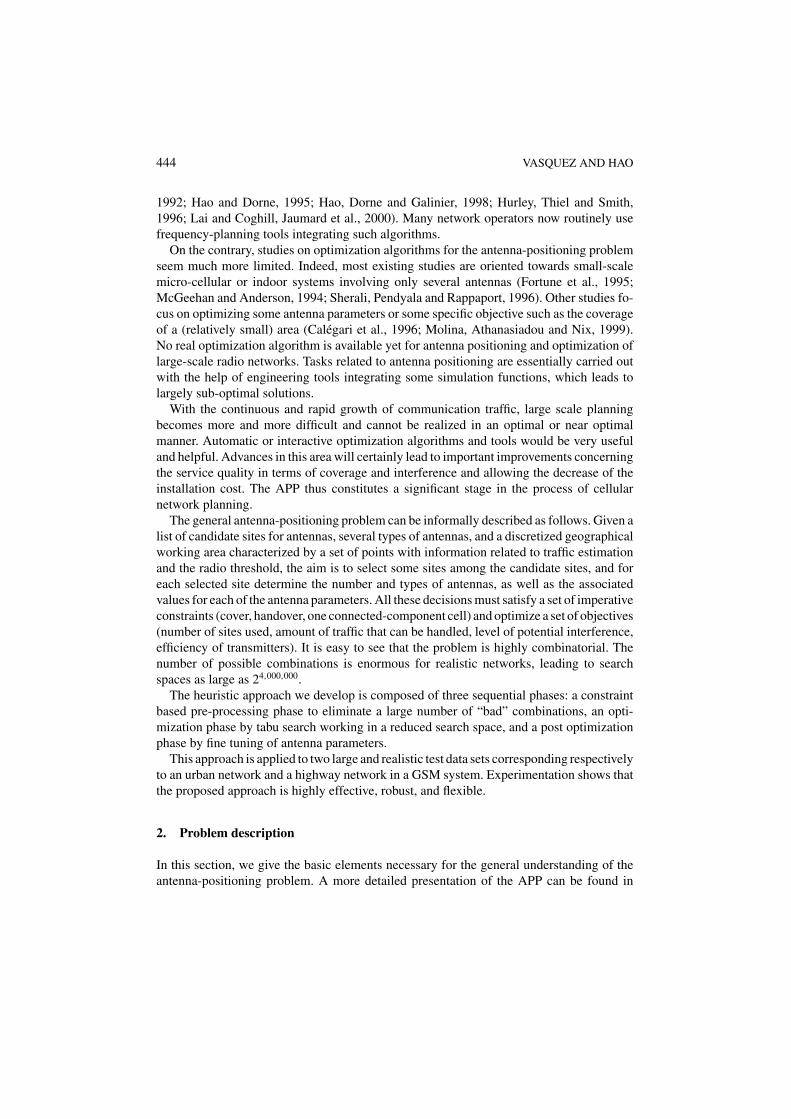
In general, there are several types of antennas available in a network, characterized primarilyby their transmission gain (Gs) and their propagation diagrams (figure 2). In this work, weconsider 3 types of antennas: omnidirectional (OMNI), large directional (LD), and smalldirectional (SD).
The principal parameters of these antennas are:
• the power, PS, which can vary from 26 to 55 dBm,• the azimuth (for a directional antenna) between 0◦ and 360◦,• the tilt (for a directional antenna) between −15◦ and 0◦,
A HEURISTIC APPROACH FOR ANTENNA POSITIONING 447
Figure 2. 3 types of antennas.
• the number of transmitters (TRX) assigned to the antenna for a given traffic. In a GSMsystem, a conversion table determines this number according to the material used. Table 3shows such an example where an antenna may require 1 to 7 TRX (thus 1 to 7 channels).Note that the number of TRX is directly determined by the traffic and does not need tobe tuned by the optimization algorithm.
These antennas can be placed on pre-defined candidate sites in the working area. In ourcase, a site can host either one OMNI antenna or one to three LD or SD antennas.
2.4. Base station and cell
A base station, BS b, is defined by a quintuplet b = (site, antenna, tilt, azimuth, power). Itcorresponds thus to the choice of a site, an antenna on this site and the parameter values of theantenna. For example, for the above network, the BS b = (356, LD, 0, 30, 38) correspondsto the placement of a LD antenna on the site numbered 356. This antenna has a tilt of 0◦,an azimuth of 30◦, and a power of 38 dBm.
Other components are also involved in the definition of a BS, such as BS transmitterloss and BS receiver sensibility (Reininger, 1997; Reininger and Caminada, 1998a), and thesame applies to the MS (Section 2.2). Since these values are constant for a given situation,they will not be further discussed in this paper.
In order to assess the signal quality at each point, a radio wave propagation model isneeded. Such a model is able to predict the propagation loss of an electromagnetic fieldbetween a site and each RTP of the working area. To compute the prediction, the modeltakes into account the site coordinates, its height, the RTP coordinates, the set of obstaclesbetween the site and the RTP (buildings, mountains...), and the angle of incidence betweenthe site and the RTP.
Table 3. Number of transmitters and traffic capacities.
TRX 1 2 3 4 5 6 7
Erlang 2.9 8.2 15 22 28 35.5 43
448 VASQUEZ AND HAO
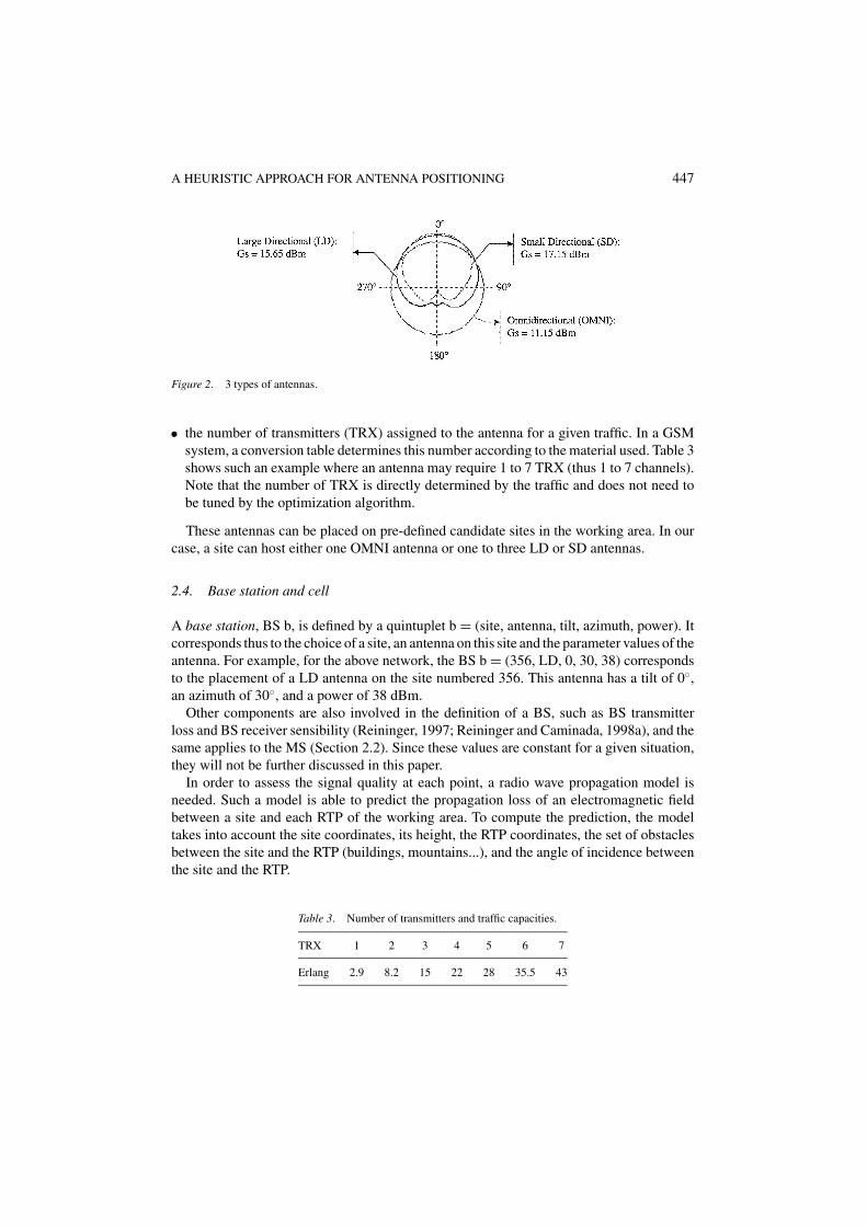
Figure 3. Cell corresponding to b = (356, LD, 0, 30, 38).
We evoked above only downlink signals emitted by base stations towards cellular phones.In fact, it is also necessary to take into account signals from MS towards BS (uplink signals).It is, however, shown in Reininger and Caminada (1998a) that if the downlink signal, comingfrom a BS, is higher than the quality threshold Sq and the uplink signal is stronger than thedownlink signal (which is indeed the case in GSM systems), then it is not necessary to beconcerned with uplink signals.
Thus, starting from the data of a BS in a network we will be able to calculate, for eachpoint of the geographical area, a radio signal, noted hereafter as Cd. The cell of a BScorresponds thus to the set of STP covered by the BS, i.e. for which the signal receivedfrom this BS is the best one and higher than the quality threshold Sq. Figure 3 illustratesthe link between an isolated BS and its cell.
Since radio wave propagation is never homogeneous and isotropic, the cell of aBS is always irregularly bounded, depending on the topography and the transmittingpower. Moreover, the cell of a BS is dependant on other BS emitting from overlappingareas.1
2.5. Constraints
Each STP must be served by at least one BS. Therefore, the union of the cells in a givennetwork must be equal to the set of all the STP located in the working area. This necessityconstitutes the global coverage constraint for a network.
When an MS moves from one cell to another, the network must be able to guaran-tee the continuity of the communication. To accomplish this, it is essential that eachcell has a nonempty intersection (handover area) with its neighboring cells. This require-ment constitutes the handover constraint, which must be respected by all the cells of thenetwork.
The STP contained in a cell may constitute several connected components. Connectedcomponents play a significant (and negative) role in the quality of a network (Reiningerand Caminada, 1998b): the more connected components there are for a cell, the more in-terference there may be. Also, cells having more connected components make it difficultto manager the handover. Therefore, one of the constraints of the APP is that each cellof the network constitutes only one connected component. This local constraint is calledone connected component (OCC) constraint, for which in this paper, only components
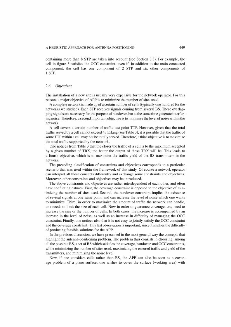
A HEURISTIC APPROACH FOR ANTENNA POSITIONING 449
containing more than 8 STP are taken into account (see Section 3.3). For example, thecell in figure 3 satisfies the OCC constraint, even if, in addition to the main connectedcomponent, the cell has one component of 2 STP and six other components of1 STP.
2.6. Objectives
The installation of a new site is usually very expensive for the network operator. For thisreason, a major objective of APP is to minimize the number of sites used.
A complete network is made up of a certain number of cells (typically one hundred for thenetworks we studied). Each STP receives signals coming from several BS. These overlap-ping signals are necessary for the purpose of handover, but at the same time generate interfer-ing noise. Therefore, a second important objective is to minimize the level of noise within thenetwork.
A cell covers a certain number of traffic test point TTP. However, given that the totaltraffic served by a cell cannot exceed 43 Erlang (see Table 3), it is possible that the traffic ofsome TTP within a cell may not be totally served. Therefore, a third objective is to maximizethe total traffic supported by the network.
One notices from Table 3 that the closer the traffic of a cell is to the maximum acceptedby a given number of TRX, the better the output of these TRX will be. This leads toa fourth objective, which is to maximize the traffic yield of the BS transmitters in thenetwork.
The preceding classification of constraints and objectives corresponds to a particularscenario that was used within the framework of this study. Of course a network operatorcan interpret all these concepts differently and exchange some constraints and objectives.Moreover, other constraints and objectives may be introduced.
The above constraints and objectives are rather interdependent of each other, and oftenhave conflicting natures. First, the coverage constraint is opposed to the objective of min-imizing the number of sites used. Second, the handover constraint implies the existenceof several signals at one same point, and can increase the level of noise which one wantsto minimize. Third, in order to maximize the amount of traffic the network can handle,one needs to limit the size of each cell. Now in order to guarantee coverage, one need toincrease the size or the number of cells. In both cases, the increase is accompanied by anincrease in the level of noise, as well as an increase in difficulty of managing the OCCconstraint. Finally, one notices also that it is not easy to jointly satisfy the OCC constraintand the coverage constraint. This last observation is important, since it implies the difficultyof producing feasible solutions for the APP.
In the previous discussion, we have presented in the most general way the concepts thathighlight the antenna-positioning problem. The problem thus consists in choosing, amongall the possible BS, a set of BS which satisfies the coverage, handover, and OCC constraints,while minimizing the number of sites used, maximizing the ensured traffic and yield of thetransmitters, and minimizing the noise level.
Now, if one considers cells rather than BS, the APP can also be seen as a cover-age problem of a plane surface: one wishes to cover the surface (working area) with
450 VASQUEZ AND HAO
various forms of cells with multiple constraints between these forms, while optimizing theobjectives.
3. Formulation of problem
In this part, the mathematical model for the APP used in this work is presented. The detailsof this model can be found in Reininger (1997), Reininger and Caminada (1998a, 1998b).The model shown here reflects only a particular scenario. Other models are surely possible.However, the basic idea of the heuristic approach presented in this paper may be applied toother scenarios.
3.1. Basic notations
• ST set of all the service test points STP in the working area,• Sq service threshold defined by a power value for a given station (Table 2),• Sm cellular phone station receiver sensitivity defined by a power value,• TT set of the traffic test points TTP of the working area: T T ⊂ ST ,• Ps antenna power,• BS quintuplet (site, antenna, tilt, azimuth, Ps),• BS1 set of selected BS that correspond to a network design,• Cdb,p field strength received at a STT p ∈ STP from a BS b ∈ BS1,• L set of the candidate sites for a given network,
The positioning of an antenna corresponds to the choice of a finite number of BS, denotedby BS1, chosen among all possible ones.
For each b belonging to BS1 we define its cell Cell(b) as follows:
Cell(b) = {p ∈ ST/Cdb,p ≥ Sq and ∀b′ ∈ BS1 b′ �= b Cdb,p > Cdb′,p}
The second part of this definition is important. It indicates that the cell of a BS depends notonly on this BS but also on the other BS in the network.
3.2. Coverage constraint
All the STP of the working area must be covered by an antenna. This constraint is formallyexpressed by the following formula:
ST =⋃
b ∈ BS1
Cell(b) (1)
3.3. One connected component (OCC) constraint
Each cell defined by a BS b must have only one connected component. If we define Cb thenumber of connected components of Cell(b), this constraint is expressed by the following
A HEURISTIC APPROACH FOR ANTENNA POSITIONING 451
Figure 4. Connected components of a single cell.
formula:
∀b ∈ BS1 Cb = 1 (2)
In this work, we do not take into account components containing fewer than MINC STP.MINC is an integer parameter to be fixed. In this study, MINC = 9 is used.2 Figure 4illustrates this principle.
One notices that the OCC constraint would be difficult to satisfy if the coverage constraintis taken into account at the same time. Indeed, when one adds a BS or increases the size ofa cell to get a larger cover, one may “cut” a one CC cell into two cells or create a cell ofmultiple components.
3.4. Handover constraint
The handover area of a cell is defined by the set of STP p covered by the BS b, such thatthere is at least one other BS b′, from which the field strength Cdb′,p on p is greater than thethreshold Sq, and at most 7 dBm above or below the field strength Cdb,p received from theBS b, or:
handCell(b) = {p ∈ Cell(b)/∃ b′ ∈ BS1 and Cdb′,p ≥ Sq and
|Cdb,p−Cdb′,p| ≤ 7dBm}
The handover constraint, which requires a non-empty handover area for each cell, isexpressed by the following formula:
∀b ∈ BS1 handCell(b) �= ✐✚ (3)
One notices that the model does not take into account the location and the number ofhandover points (Reininger and Caminada, 1998a). This definition corresponds in fact to a

452 VASQUEZ AND HAO
weak form of the handover requirement (number of minimal handover point = 1 per cell) andmay be easily extended to include more than one minimal handover points. Computationalsimulations show that this weak form of handover is sufficient to ensure good handover ina network when the coverage constraint is satisfied. This observation may be interpreted asan indicator that the coverage constraint implies somewhat handover. We observe also thatthe handover constraint defined by (3) is satisfied as soon as there are a sufficient numberof cells in the network.
3.5. Minimize the number of sites used
This objective is defined by:
min∑i∈L
ci × yi , yi ={
1, if site i is selected
0, otherwise(4)
ci is the cost of site i . In this paper, we suppose all the sites have a unit cost:3
∀i ∈ L , ci = l
This restriction corresponds to networks in construction. There are, however, networks inextension for which the cost of a site depends on the operation that one carries out: creationof a new site, modification or suppression of an existing site in the initial network. We willdiscuss this point in the conclusion section and show that the resolution approach presentedin the paper remains valid in this situation.
3.6. Minimize the noise level
Noise level estimation is not straightforward. If there is too much overlap between cells,noise level will be very high. We have defined a cell as the set of STP with the best signalcoming from the same BS b. So Cdb,p is the best signal received at a given point p ofthe cell Cell(b). Ideally, each STP of Cell(b) should not receive more than h signals lowerthan Cdb,p and greater than the required sensitivity threshold Sm (Section 2.2.). These hsignals are used for handover. In our work, h value is fixed at 3, but it is a parameter thatcan be varied according to the model used. Signals after the hth and greater than Sm areconsidered as noise. For each point p of Cell(b), consider the sorted list of signals greaterthan Sm:
Cdb,p ≥ Cdb1,p ≥ · · · Cdbh,p ≥ · · · Cdbk,p > Sm
Hence the noise level at point p is given by:
ϒ(p) =∑
h< j≤k
Cdbj, p − Sm (k is dependent on p)
A HEURISTIC APPROACH FOR ANTENNA POSITIONING 453
The objective of minimizing the total amount of noise is expressed as follows:
min∑p∈ST
ϒ(p) (5)
3.7. Maximize the amount of traffic of the network
The total traffic a BS b can handle is given by the following formula:
traffic BS (b) =∑
p∈T T ∩Cell(b)
traffic point(p)
According to this value, one will assign a number of transmitters TRX to this station byusing the conversion Table 3. If the total traffic required by the TTP of a BS exceeds 43Erlang, then the exceeding traffic may be lost. It is for this reason that we introduce theconcept of the traffic hold of a cell:
trafficHold(b) ={
traffic(b) if (traffic(b) ≤ 43),
43 otherwise.
The objective of maximizing the amount of traffic hold of a network is expressed by:
max∑
b∈BS1
trafficHold(b) (6)
3.8. Maximize traffic yield
Given the traffic hold of a BS b and the traffic capacity of b (see Section 2.3 and Table 3),we define the traffic yield for a cell by:
trafficYield(b) = trafficHold(b)
trafficCapacity(b)
Hence, the objective of maximizing the traffic yield is expressed by the following formula:
max∑
b∈BS1
trafficYield(b) (7)
4. Problem analysis
This section presents the main characteristics of the APP, allowing us to have an ideaabout the difficulty of the problem. These characteristics are: a very high number of
454 VASQUEZ AND HAO
search combinations, a high complexity of computation, and a high requirement ofmemory.
4.1. Large number of combinations
The values of the parameters of antennas were discretized as follows:
• Ps ∈ [26..55] and δPs = 2 dBm → |Ps| = 15,• azimuth ∈ [0..359] and δazimuth = 10◦ → |azimuth| = 36,• tilt ∈ [−15..0] and δtilt = 3◦ → |tilt| = 6.
These values were considered to be sufficient for the precision of calculations and theresolution of the problems. This quantification is a first step towards reducing the numberof search combinations.
Thus, an omnidirectional antenna has |Ps| = 15 possible settings, and a directionalone has |Ps| × |azimuth| × |tilt| = 3240 possible settings. Thus, to put a BS at a site, wehave 15 + 3240 + 3240 = 6495 possible choices (denoted by |BSsite|). If |L| representsthe number of candidate sites of a network number of candidate sites, we get |L| × |BSsite|possible choices for a BS in the network.
To build a network is to find a combination of base stations, among the possible |L| ×|BSsite| ones, which satisfies all the constraints and optimizes the objectives. We thus have2|L| × |BSsite| potential choices of configurations, even if a large number of them are notfeasible.
For example, the network of figure 1 has 568 candidate sites, and thus a search space of2568 × 6495 = 23,689,160 combinations.
4.2. Computational complexity
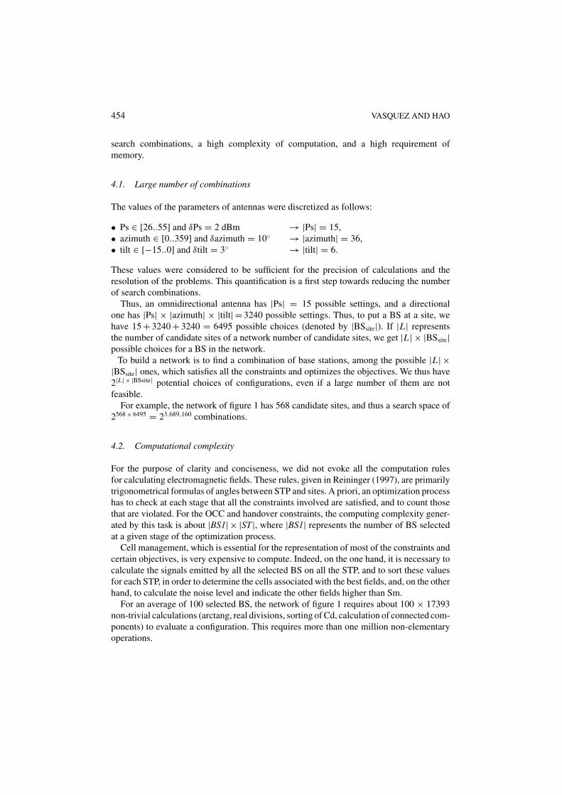
For the purpose of clarity and conciseness, we did not evoke all the computation rulesfor calculating electromagnetic fields. These rules, given in Reininger (1997), are primarilytrigonometrical formulas of angles between STP and sites. A priori, an optimization processhas to check at each stage that all the constraints involved are satisfied, and to count thosethat are violated. For the OCC and handover constraints, the computing complexity gener-ated by this task is about |BS1| × |ST|, where |BS1| represents the number of BS selectedat a given stage of the optimization process.
Cell management, which is essential for the representation of most of the constraints andcertain objectives, is very expensive to compute. Indeed, on the one hand, it is necessary tocalculate the signals emitted by all the selected BS on all the STP, and to sort these valuesfor each STP, in order to determine the cells associated with the best fields, and, on the otherhand, to calculate the noise level and indicate the other fields higher than Sm.
For an average of 100 selected BS, the network of figure 1 requires about 100 × 17393non-trivial calculations (arctang, real divisions, sorting of Cd, calculation of connected com-ponents) to evaluate a configuration. This requires more than one million non-elementaryoperations.

A HEURISTIC APPROACH FOR ANTENNA POSITIONING 455
Table 4. Data for the APP.
Set of candidate sites: L |L| ∼ 500
Set of RTP: R |R| ∼ 100000
Set of STP From 10000 to 100000
Set of TTP From 5000 to 100000
Propagation loss matrix |L| × |R|Angle of incidence matrix |L| × |R|
4.3. Memory consumption
Computing the signals dynamically using a radio propagation model is very time consuming,and, therefore, cannot be used during an optimization process. Propagation loss data arethus pre-computed and stored in a propagation loss matrix where propagation loss has beenpredicted from each site to each RTP. Associated to these values we have an incidencematrix that gives the incidence angle for each couple (site, RTP). For each type of antenna,we also have the horizontal and vertical diagrams. Using this data, one can compute thefield strength Cdb,p by using the formulas detailed in Reininger (1997). Table 4 gives anidea about the quantity of data necessary for the problems that we solved.
Typically, the data concerning the radio signal, the values of traffic, the coordinates ofthe sites, and the points of a network require more than 200 MB of memory.
5. General heuristic approach for the APP
The APP is thus highly combinatorial and very difficult to resolve. This remains true even forfinding feasible solutions satisfying all the constraints. In particular, it is not at all obvioushow the OCC and coverage constraints can be satisfied simultaneously.
To tackle the APP, we have developed a heuristic approach, which is composed of threesequential phases: a pre-processing phase based on a filtering principle, an optimizationphase based on tabu search, and a post-optimization phase by fine tuning antenna para-meters.
The pre-processing phase uses some filtering criteria to eliminate or filter out manyundesirable base stations (or cells) that cannot contribute to a good solution. We calculate,site by site and antenna by antenna, all the possible cells generated by each BS (site, antenna,power, tilt, azimuth). According to the filtering criteria, we decide for each cell whether thecell is kept or rejected. For example, if the filtering criterion used is the OCC constraint,then any cell violating this constraint will be definitively eliminated. Similarly, if we wantto limit the size of the cells, we may use this criterion to filter out the cells exceeding thedesired size. Therefore, this pre-processing step allows us to greatly reduce the number ofcombinations of the search space. For network such as the one we used, this step retainstypically 200,000 to 400,000 BS, from some 4,000,000 possible ones. Let us notice anotherimportant point: Computations of field strengths for each point in the working area are
456 VASQUEZ AND HAO
carried out at this phase and are no longer necessary during the optimization phase whichis carried out by tabu search.
From the set of BS produced by the pre-processing phase, the optimization phase by tabusearch will construct solutions by choosing a subset of BS that satisfy all the constraintsof the problem and optimize the objectives. To do this, the tabu algorithm, starting withan empty solution, tries to extend at each iteration its current solution by adding a BS anddropping some existing BS, if necessary, (for instance, to continue satisfying the OCC con-straint). The choice of which BS is added at each iteration takes into account the objectives,and checks that the coverage constraint is satisfied.
Finally, the post-optimization phase is applied to improve the solution produced bythe tabu algorithm. This phase can be used to optimize objectives or repair the rare con-straints that remain unsatisfied. Post-optimization is realized by the fine-tuning of antennaparameters.
6. Pre-processing
6.1. Constraint based pre-processing
As previously mentioned, one of the main difficulties of the APP concerns the managementof the OCC and coverage constraints. One well-known technique for constraint handlingin general is the penalty-based approach. In this approach, constraints are considered asobjectives and integrated into a weighted evaluation function:
f ′ =i=m∑i=1
fi +i=n∑j=1
pj × �(cj )
where:
• fi represents one initial objective,• pj is a penalty to be defined for constraint cj,• �(cj ) equals 1 if cj is satisfied, equals 0 otherwise.
An advantage of this approach lies its flexibility, while its main drawback is the difficultyin fine tuning the penalties. Indeed, if some constraints are incompatible and hard to satisfy,these constraints may never be satisfied. This is precisely the case for the OCC and coverageconstraints.
To cope with this difficulty, we introduce a special technique for handling the OCC con-straint (the global coverage constraint is handled with the penalty approach, see Section 7.2).The basic idea is to use the OCC constraint in an active way to filter out “bad” BS whichviolate this constraint, and which consequently cannot contribute to a good solution. Only“good” BS are retained.
Recall that a candidate site can host one omnidirectional (OMNI) antenna or one to threedirectional (LD or SD) antennas, which results in 6495 potential base stations. For a givensite, all its BS configurations are not of equal interest. In particular, a BS whose cell has
A HEURISTIC APPROACH FOR ANTENNA POSITIONING 457
many connected components can in no way be useful for a final solution due to the OCCconstraint. Therefore, it would be beneficial to eliminate such BS from the search space fromthe beginning. That is what we do during the pre-processing phase. For every possible BS b= (site, antenna, power, tilt, azimuth) of every candidate site, we carry out all the necessarycomputations of field strengths to calculate the corresponding cell of the BS, and then countthe number of its connected components having more than 9 STP (see Section 3.3). If thenumber of connected components is greater than one, i.e. the OCC constraint is violated,then the cell is not counted. Otherwise, the cell is recorded in a data structure together withall related information. Therefore, the left cell in figure 4 (Section 3.3) is kept, while theright one is rejected.
To calculate the connected components, we use the “scan line blob coloring algorithm”,which is well known in the field of computer vision (Ballard and Ballard, 1982). Thisalgorithm scans the working area from top left to bottom right and labels STP belongingto the same cell with the same color. To accomplish this, it considers four points aroundthe current one: the three neighboring points on top and the left neighboring point in an8-neighborhood. For a single BS, this algorithm has a time complexity of O(|Cell(b)|).
This OCC constraint-based pre-processing phase allows one to significantly reduce thesize of the search space, especially in the situations where many irregular obstacles arepresent in the terrain. Indeed for the network of figure 1, this filtering step retains only 294000BS. The combinations in our search space are thus reduced from 23689160 (intractable) to2294000 (tractable).
The idea behind the pre-processing is very general and other criteria, like the noise leveland the traffic, can be easily used separately or conjointly for this pre-processing phase.Such pre-processing techniques were implemented and experimented upon in our study.However, we are unable to describe them further within the framework of this paper.
Therefore, the pre-processing phase offers great flexibility, allowing us to generate manydifferent search spaces with different characteristics, which can then be used by the opti-mization phase to produce various solutions. This flexibility represents a nice feature formulti-objective optimization problems such as the APP.
6.2. Connectivity constraint transformation
After this filtering stage, we have cells which satisfy the OCC constraint individually, andwhich have additional proprieties when other filtering criteria are applied. Since the OCC isdifficult to handle, this constraint must remain satisfied during the tabu optimization phase,which consists in adding and dropping BS. For this purpose, we divide each cell into twoparts, called the “kernel” and “border,” and introduce a new constraint called the “kernelconstraint.”
Let δSq be a dBm value greater than 0: δSq > 0 dBm. For each cell, one considers the 2following sets:
kernel(b) = {p ∈ Cell(b)/Sq + δSq ≤ Cdb,p}border(b) = {p ∈ Cell(b)/Sq ≤ Cdb,p < Sq + δSq}
Figure 5 illustrates this partition.

458 VASQUEZ AND HAO
Figure 5. Cell = {border} ∪ {kernel}.
Then the kernel constraint states that the kernels of two different cells do not overlap:
∀(b, b′) ∈ BS1 × BS1, b �= b′ ⇒ kernel(b) ∩ kernel(b′) = ✐✚
Notice that the partition of a cell into kernel and border may be adjusted by the valuegiven to δSq. By varying the value of δSq, we can make the kernel constraint stronger orweaker.
Now, during the tabu optimization phase, this kernel constraint is used so that the OCCconstraint will remain satisfied. Therefore, the management of the OCC is replaced byhandling this simpler kernel constraint.
The kernel constraint does not forbid the overlapping of the border zone of one cell withthat of another cell. Such an overlapping zone is typically used to ensure the handoverconstraint.
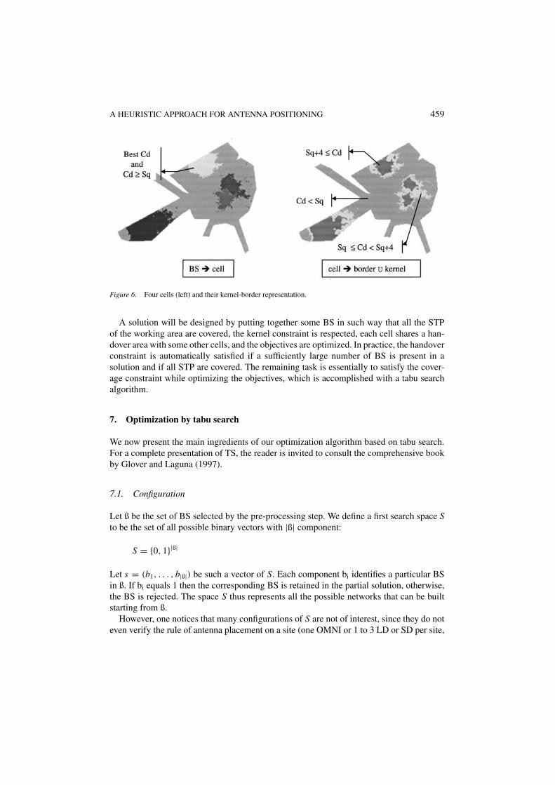
Let us now consider a more detailed example. Table 5 shows a partial solution involving4 BS. Figure 6 gives the cells of these BS (left) together with their kernel and borders (right).In this example, δSq = 4 dBm is used to defined the border areas. One notices that theoverlap of the two adjacent cells concerns only their borders.
In summary, the pre-processing step generates, from the raw data of the problem, areduced set of BS, as well as their representation in terms of kernel and border. The nextstep consists in constructing a solution from these BS.
Table 5. A partial configuration for the urbannetwork.
Site Antenna Tilt Azimut Ps
131 LD 0 90 46
356 LD 0 30 38
397 LD −6 300 46
493 SD −6 90 50
A HEURISTIC APPROACH FOR ANTENNA POSITIONING 459
Figure 6. Four cells (left) and their kernel-border representation.
A solution will be designed by putting together some BS in such way that all the STPof the working area are covered, the kernel constraint is respected, each cell shares a han-dover area with some other cells, and the objectives are optimized. In practice, the handoverconstraint is automatically satisfied if a sufficiently large number of BS is present in asolution and if all STP are covered. The remaining task is essentially to satisfy the cover-age constraint while optimizing the objectives, which is accomplished with a tabu searchalgorithm.
7. Optimization by tabu search
We now present the main ingredients of our optimization algorithm based on tabu search.For a complete presentation of TS, the reader is invited to consult the comprehensive bookby Glover and Laguna (1997).
7.1. Configuration
Let ß be the set of BS selected by the pre-processing step. We define a first search space Sto be the set of all possible binary vectors with |ß| component:
S = {0, 1}|ß|
Let s = (b1, . . . , b|ß|) be such a vector of S. Each component bi identifies a particular BSin ß. If bi equals 1 then the corresponding BS is retained in the partial solution, otherwise,the BS is rejected. The space S thus represents all the possible networks that can be builtstarting from ß.
However, one notices that many configurations of S are not of interest, since they do noteven verify the rule of antenna placement on a site (one OMNI or 1 to 3 LD or SD per site,

460 VASQUEZ AND HAO
see Section 2.3). To translate this implicit constraint of the model we associate with eachtype of antenna a weight ρ:
ρ :
ρ(OMNI) = 3,
ρ(LD) = 1,
ρ(SD) = 1.
For a BS b we use ρ(b) to denote the value ρ (b antenna type) and define the followingfunction:
As : S × L �→ {0, 1, . . .} As(s, l) =∑
b=1 and b on site 1
ρ(b)
We now define the subspace T ⊂ S verifying the rule of antenna placement on a site:
T = {s ∈ S/∀l ∈ L As(s, l) ≤ 3}
It is clear that this reduced search space is of greater interest than the initial space S.From T we now define a last search space X ⊂ T that respects the kernel constraint
(Section 6.2):
X = {(b1, . . . , b|ß|
) ∈ T/∀i , ∀j, i �= j and bi = 1 and b j = 1
⇒ kernel(bi ) ∩ kernel(b j ) = ✐✚}
Therefore, the search space X includes all the configurations that satisfy both the rule of an-tenna positioning on a site and the kernel constraint. Since many non feasible configurationsare excluded from X compared with the initial search space, we have |X | � |S|.
7.2. Configuration evaluation
In order to guide the tabu algorithm to visit the search space, one needs a function forevaluating the configurations. Since the APP involves multiple objectives and multipleconstraints, the evaluation is somewhat complicated. In this work, we took a hierarchicalapproach to evaluate the configurations. Formally, for a given configuration s of X , itis evaluated by the following vector function.
ξ(s) = 〈c0(s), f1(s), f2(s), f3(s), f4(s)〉 where :
• c0(s) = coverage(s) = number of STP covered by the cells of s,• f1(s) = trafficHold(s) = sum of traffic held by all the cells of s,• f2(s) = noise(s) = sum of noise generated by each selected BS of s,• f3(s) = number of sites where BS are installed,• f4(s) = traffic Yield(s).

A HEURISTIC APPROACH FOR ANTENNA POSITIONING 461
The first component c0 of this evaluation function corresponds to the coverage constraint.This component takes priority over the other components (f1, f2, f3 and f4) that are related tothe different objectives of the problem. A higher priority for the component c0 helps toguide the search to find first feasible solutions. Another possibility would consider thecomponent c0 at the same level as the other objectives at the risk of never finding a feasiblesolution.
For the components f1, f2, f3 and f4, any priority order may be used according to the im-portance we give to each objective. For our presentation, we chose arbitrarily the followingpriority order P:
P(f1) > P(f2) > P(f3) > P(f4)
Given two configurations s1 and s2, s1 is said to be better than s2, denoted by ξ(s1) > ξ(s2),if the following condition is verified:
ξ(s1) > ξ(s2) ⇔
(c0(s1) > c0(s2)) or,
(c0(s1) = c0(s2) and f1(s1) > f1(s2)) or,
(c0(s1) = c0(s2) and f1(s1) = f1(s2) and f2(s1) < f2(s2)) or,
. . .
�ξ(s1,s2) = 〈�c0(s1,s2), �f1(s1,s2), �f2(s1,s2), �f3(s1,s2), �f4(s1,s2)〉 denotes thevector variation of ξ .
We also use another function of evaluation: ξ ′(s) = 〈c′0(s), f1(s), f2(s), f3(s), f4(s)〉 where:
c′0(s) =
∑pcovered
w(p) where w(p) is a weight value greater than 0, and
ξ ′(s) ⇔ ξ(s) if w(p) = 1 ∀ p ∈ ST.
We will see the usefulness of this evaluation function in Section 7.5.
7.3. Neighborhood and move
We now introduce the neighborhood function N over the search space X . More precisely,this function N : X → 2X is defined as follows.
Let s = (b1, b2, . . . , b|ß|) ∈ X and s′ = (b′1, b′
2, b′|ß|) ∈ X then s′ is a neighbor of s, i.e.
s′ ∈ N(s), if and only if the following conditions are met:
1) ∃ ! i such that bi = 0 and b′i = 1 (1 ≤ i ≤ |ß|)
2) for the above i, ∀ j �=i ∈ {1 . . . |ß|} kernel (bi) ∩ kernel (bj) �= ✐✚ ⇒ b′j = 0
Thus, a neighbor of s can be obtained by adding a BS (flipping a variable bi from 0 to 1) inthe current configuration and then dropping some other BS (flipping some bj from 1 to 0) torepair the kernel constraint violation. Consequently, a move mv to obtain a neighbor s′ from
462 VASQUEZ AND HAO
a configuration s = (b1, b2, b3 . . . b|ß|) is characterized by a series of flipping operations:
bi from 0 to 1
bi1 from 1 to 0
. . . . . .
bin from 1 to 0
where bi1 . . . bin are variables linked to bi by the kernel constraint. That means that there is atleast one same element (i.e. STP) in both kernel (bi) and kernel(bj) for j ∈ Ji = {i1, . . . , in}.Such a moved is denoted by mv(i) = (bi : 0→1, bj1 . . . bin : 1→0). Use s′ = s + mv(i) todenote the neighbor of s obtained by applying mv(i) to s.
It should be clear that from a configuration s = (b1, b2, . . . , b|ß|), there are as manypossible moves as the number of variables in s having a value of 0.
Let |s| = ∑1≤i≤|ß| bi , then s has exactly |ß| − |s| neighboring configurations (i.e. |N(s)| =
|ß|−|s|).
7.4. Tabu list management and aspiration criteria
The main role of a tabu list is to prevent the search from short-term cycling (bj : 1 → 0 →1 → 0 . . .). Given the considerable quantity of calculations to be carried out for a move,we avoid immediately dropping a BS that has just been selected. To do this, a simplefrequency-based mechanism is used:
Let Freq(i) be the frequency of a move mv(i) (i.e. the number of times the BS bi is selectedin the partial solution), then the number of iterations during which an element bi should notbe reset to 0 is equal to Freq(i). The number is called tabu tenure of the move mv(i).
In order to implement the tabu list, a vector Tabu of |ß| elements is used. As suggested inGlover and Lugana (1997), each element Tabu(i), i.e. the tabu tenure of mv(i) (1 ≤ i ≤ |ß|)records Freq(i) + t where t is the number of iterations when mv(i) is carried out. In thisway, it is quite easy to know, at a later iteration t ′, if a mv(i) is allowed or not: if there existsj ∈ Ji = {i1 . . . in} such that Tabu(j) > t ′ then mv(i) is a forbidden move, otherwise, mv(i)is a possible move.
The tabu status of a move mv(i), such that s′ = s + mv(i), is canceled if s′ has a bet-ter quality than s, i.e. ξ(s′) > ξ(s). This condition corresponds to a simple, yet importanttechnique called “aspiration criteria.”
7.5. Diversification
During the normal search process, the tabu algorithm chooses, at each iteration, one bestmove among all possible moves. This process is stopped and a diversification phase istriggered if no improved configuration is found during a fixed number of iterations. To dothis, we re-calculate the weight of each STP in the following way:
If the STP is already covered by a BS, its weight equals 1, otherwise, the weight equals1 + |ST |. One then replaces the evaluation function ξ by ξ ′ (Section 7.2.). The evaluation
A HEURISTIC APPROACH FOR ANTENNA POSITIONING 463
function is changed in order to focus the search on the uncovered STP. This mechanismallows the search process to escape from a local optimum.
The number of iterations that trigger a diversification is relatively small, because one doesnot want to carry out too many non-improving moves, which require many calculations.This number is determined automatically using a simple idea. When our algorithm arrivedat a local optimum, it selected |s∗| BS, |s∗| being the number of elements with 1 in s∗. Weconsider that if it carries out, from this point, |s∗| moves without improvement then it isnecessary to diversify the search.
Let us notice that during diversification, the value of c′0(s) does not represent the real
coverage ensured by the configuration s. The real coverage c0(s) is kept up to date duringthe diversification.
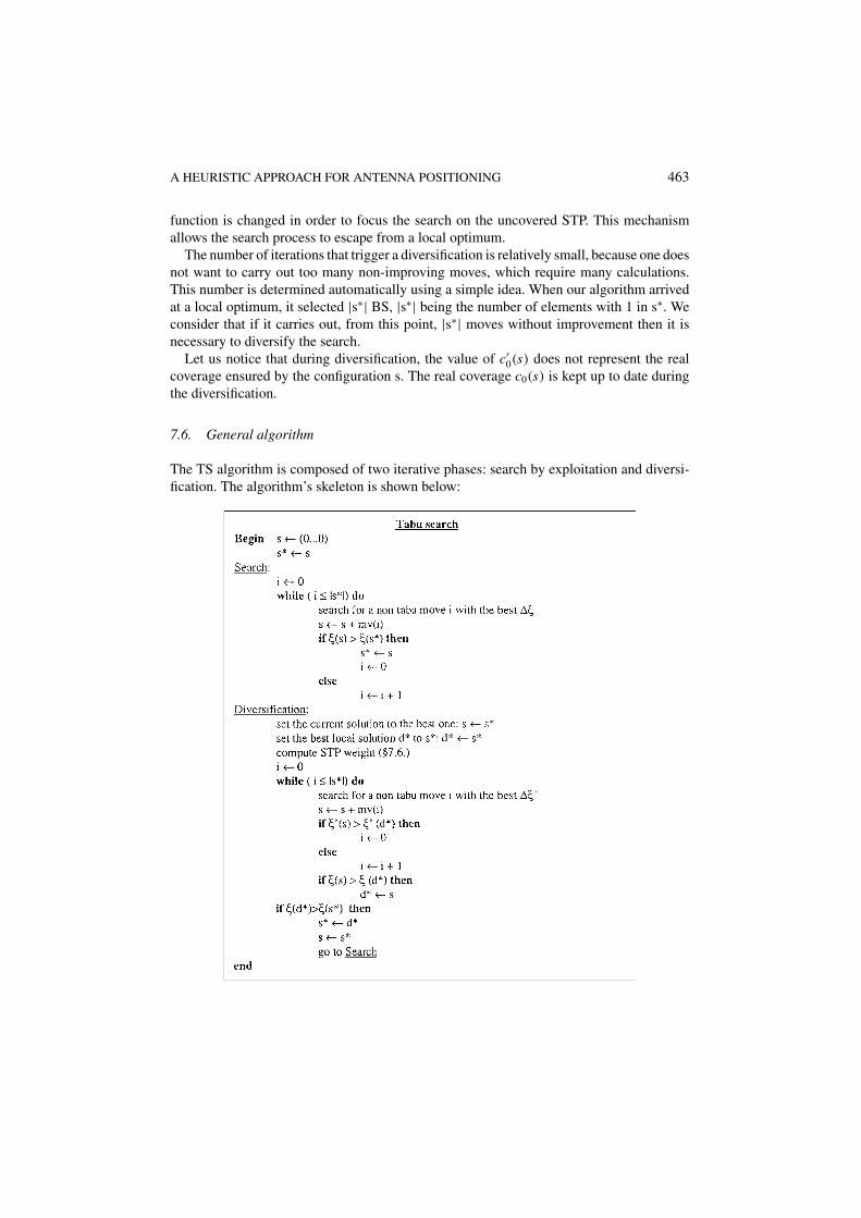
7.6. General algorithm
The TS algorithm is composed of two iterative phases: search by exploitation and diversi-fication. The algorithm’s skeleton is shown below:
464 VASQUEZ AND HAO
The tabu algorithm stops when a diversification is not able to improve the solution withwhich the diversification starts. The algorithm returns the best solution s∗ found during thesearch. This TS algorithm requires no parameter to tune. Note that, if we are only interestedin satisfying constraints, a stop condition may be added when the value of the ξ componentc0 (i.e. coverage) is equal to |ST |.
8. Post optimization
Generally speaking, the post-optimization phase can be used to optimize any objective (thenoise level, the total traffic supported . . . ) or to enhance constraint satisfaction in case ofconstraint violation. The basic idea of the post-optimization phase is to improve a solutionby fine tuning some antenna parameters.
As discussed in this paper, it is very difficult to satisfy the coverage and OCC constraintssimultaneously. The proposed approach satisfies the OCC first and tries to satisfy the cov-erage constraint during tabu optimization. Typically, tabu optimization alone can result incoverage greater than 99%. If a 100% coverage is not reached, we use the following postoptimization technique to cover the remaining 1% of STP.
The principle of this post optimization process is simple: if one slightly increases thepower of some BS selected in such a solution s*—to almost the feasibility level—we shouldbe able to obtain the total coverage of the STP, without violating the other constraints.For this purpose, we seek the closest BS bmin of the uncovered STP (in terms of signalpower):
δCdb,p = Sq − Cdb,p(p is not covered so δCd > 0)
bmin = b ∈ BS1 / δCd is minimum
If the power (Ps) of bmin verifies the relation, Ps + δCd ≤ 55 dBm, then one can increasethe power of this BS and repeat the operation. This simple process allows us to satisfy thecoverage constraint in most cases.
Let us notice that for the post optimization phase, one may use other antenna parametersinstead of power. Moreover, this kind of tuning may be easily applied to improve an existingnetwork.
We have developed other techniques for improving objectives, such as traffic hold andnoise level. For the purpose of simplification, these techniques are not presented here.
9. Experimentation and numerical results
9.1. Data sets
Computational experiments are carried out on two large and realistic data sets correspondingto two different types of networks: an urban network and a highway network. These test setswere generated by the CNET, which is France Telecom’s research laboratory, by using a very
A HEURISTIC APPROACH FOR ANTENNA POSITIONING 465
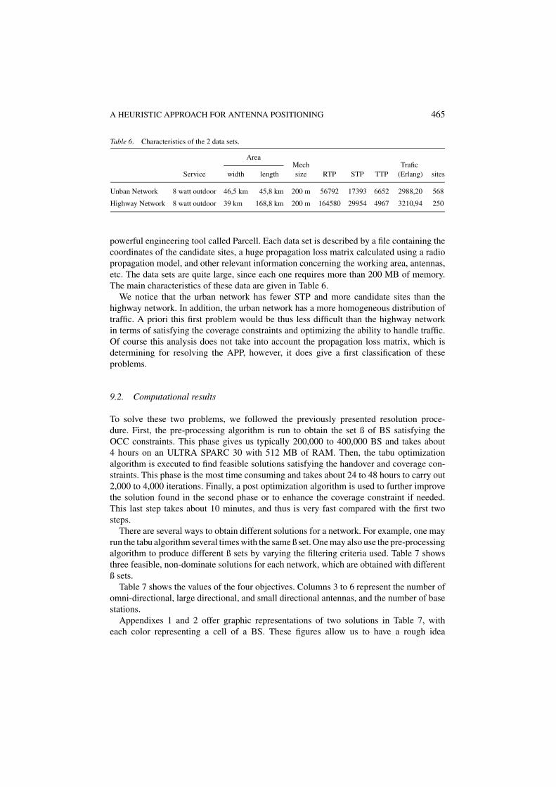
Table 6. Characteristics of the 2 data sets.
Area
Service width lengthMechsize RTP STP TTP
Trafic(Erlang) sites
Unban Network 8 watt outdoor 46,5 km 45,8 km 200 m 56792 17393 6652 2988,20 568
Highway Network 8 watt outdoor 39 km 168,8 km 200 m 164580 29954 4967 3210,94 250
powerful engineering tool called Parcell. Each data set is described by a file containing thecoordinates of the candidate sites, a huge propagation loss matrix calculated using a radiopropagation model, and other relevant information concerning the working area, antennas,etc. The data sets are quite large, since each one requires more than 200 MB of memory.The main characteristics of these data are given in Table 6.
We notice that the urban network has fewer STP and more candidate sites than thehighway network. In addition, the urban network has a more homogeneous distribution oftraffic. A priori this first problem would be thus less difficult than the highway networkin terms of satisfying the coverage constraints and optimizing the ability to handle traffic.Of course this analysis does not take into account the propagation loss matrix, which isdetermining for resolving the APP, however, it does give a first classification of theseproblems.
9.2. Computational results
To solve these two problems, we followed the previously presented resolution proce-dure. First, the pre-processing algorithm is run to obtain the set ß of BS satisfying theOCC constraints. This phase gives us typically 200,000 to 400,000 BS and takes about4 hours on an ULTRA SPARC 30 with 512 MB of RAM. Then, the tabu optimizationalgorithm is executed to find feasible solutions satisfying the handover and coverage con-straints. This phase is the most time consuming and takes about 24 to 48 hours to carry out2,000 to 4,000 iterations. Finally, a post optimization algorithm is used to further improvethe solution found in the second phase or to enhance the coverage constraint if needed.This last step takes about 10 minutes, and thus is very fast compared with the first twosteps.
There are several ways to obtain different solutions for a network. For example, one mayrun the tabu algorithm several times with the same ß set. One may also use the pre-processingalgorithm to produce different ß sets by varying the filtering criteria used. Table 7 showsthree feasible, non-dominate solutions for each network, which are obtained with differentß sets.
Table 7 shows the values of the four objectives. Columns 3 to 6 represent the number ofomni-directional, large directional, and small directional antennas, and the number of basestations.
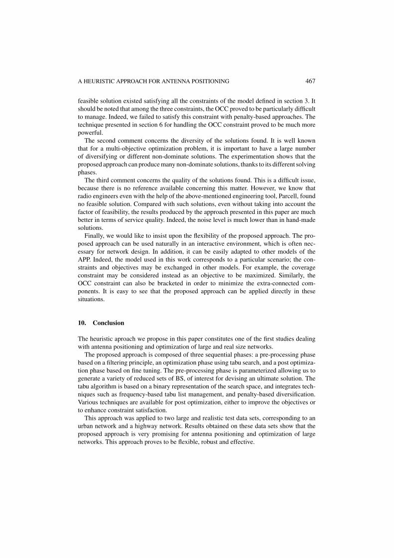
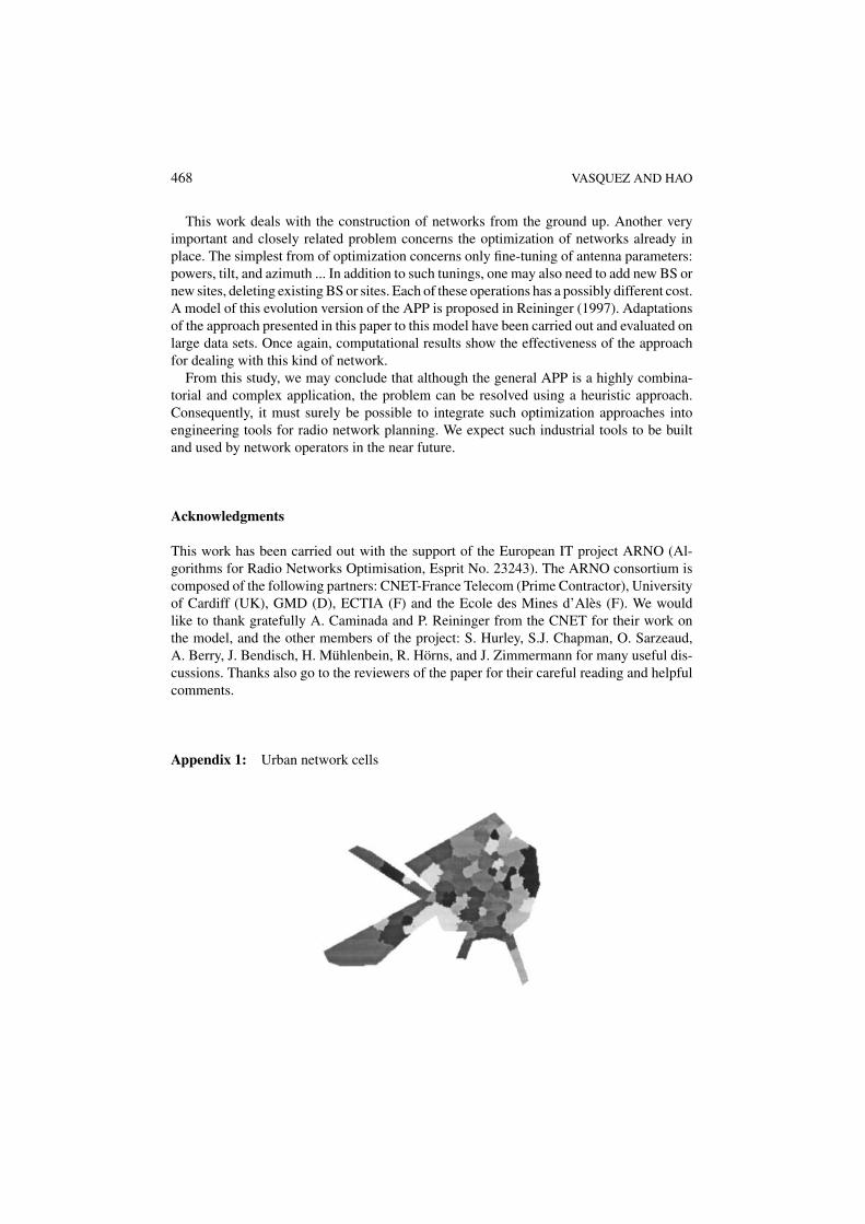
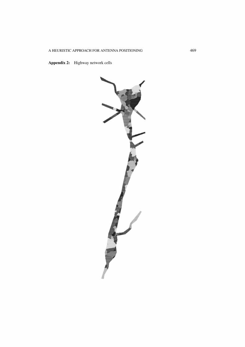
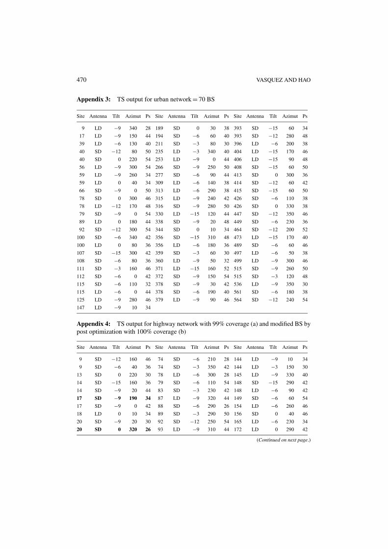
Appendixes 1 and 2 offer graphic representations of two solutions in Table 7, witheach color representing a cell of a BS. These figures allow us to have a rough idea

466 VASQUEZ AND HAO
Table 7. Feasible solutions for an urban network and a highway network.
Sites OMNI LD SD BS Noise Traffic hold Traffic yeild
Urban network 60 0 29 41 70 215135,10 2239,96 75% 62%
63 0 41 44 85 274504,5 2339,14 78% 86%
94 0 0 154 154 216460,3 2988,12 100% 78%
Highway network 58 1 35 67 103 331227,7 2251,50 70% 72%
78 0 28 128 156 385918,8 2889,55 90% 72%
86 0 39 78 117 278481,4 2797,75 87% 79%
Table 8. Unfeasible configurations for an urban network and a highway network.
OCC Sites OMNI LD SD BS Noise Traffic hold Traffic yeild
Urban network 2 63 0 0 135 135 344874,45 2940,41 98% 73%
2 89 0 134 0 134 362020,80 2953,00 99% 80%
Highway network 9 79 0 0 118 118 316644,29 3171,19 99% 80%
10 110 0 164 0 164 358675,00 3210,91 100% 78%
about the topology of the solutions found. For example, we observe that the cells arequite homogeneous, which is considered to be a desirable property of a network. Ap-pendixes 3 and 4 give the two corresponding solutions in detail. From these detailed ta-bles, we observe that the values of the “power” of antennas are rather close to the highvalue part. The repartitioning of the “tilt” values is almost homogeneous. We also ob-serve that there are very few omnidirectional antennas. This may be explained by the factthat there is neither constraint nor objective on the number of BS, and several directionalantenas can ensure the coverage of an omnidirectional antenna, with much better tuningpossibilities.
In a similar way, for each network Table 8 presents two unfeasible solutions, where theOCC constraint is relaxed (number of OCC indicated in the second column). The mainpurpose of these results is to show the flexibility of the proposed approach. By comparingthe results of Tables 7 and 8, we observe that the violation of the OCC constraint increasesthe noise level. This observation constitutes an empirical justification of the importanceof the OCC constraint.
9.3. Comments and discussions
Let us now make some comments about these results and the proposed approach. The firstcomment concerns the feasibility of solutions for these networks. Given the high complexityof the data used and the way the data has been generated, it was unknown whether any
A HEURISTIC APPROACH FOR ANTENNA POSITIONING 467
feasible solution existed satisfying all the constraints of the model defined in section 3. Itshould be noted that among the three constraints, the OCC proved to be particularly difficultto manage. Indeed, we failed to satisfy this constraint with penalty-based approaches. Thetechnique presented in section 6 for handling the OCC constraint proved to be much morepowerful.
The second comment concerns the diversity of the solutions found. It is well knownthat for a multi-objective optimization problem, it is important to have a large numberof diversifying or different non-dominate solutions. The experimentation shows that theproposed approach can produce many non-dominate solutions, thanks to its different solvingphases.
The third comment concerns the quality of the solutions found. This is a difficult issue,because there is no reference available concerning this matter. However, we know thatradio engineers even with the help of the above-mentioned engineering tool, Parcell, foundno feasible solution. Compared with such solutions, even without taking into account thefactor of feasibility, the results produced by the approach presented in this paper are muchbetter in terms of service quality. Indeed, the noise level is much lower than in hand-madesolutions.
Finally, we would like to insist upon the flexibility of the proposed approach. The pro-posed approach can be used naturally in an interactive environment, which is often nec-essary for network design. In addition, it can be easily adapted to other models of theAPP. Indeed, the model used in this work corresponds to a particular scenario; the con-straints and objectives may be exchanged in other models. For example, the coverageconstraint may be considered instead as an objective to be maximized. Similarly, theOCC constraint can also be bracketed in order to minimize the extra-connected com-ponents. It is easy to see that the proposed approach can be applied directly in thesesituations.
10. Conclusion
The heuristic aproach we propose in this paper constitutes one of the first studies dealingwith antenna positioning and optimization of large and real size networks.
The proposed approach is composed of three sequential phases: a pre-processing phasebased on a filtering principle, an optimization phase using tabu search, and a post optimiza-tion phase based on fine tuning. The pre-processing phase is parameterized allowing us togenerate a variety of reduced sets of BS, of interest for devising an ultimate solution. Thetabu algorithm is based on a binary representation of the search space, and integrates tech-niques such as frequency-based tabu list management, and penalty-based diversification.Various techniques are available for post optimization, either to improve the objectives orto enhance constraint satisfaction.
This approach was applied to two large and realistic test data sets, corresponding to anurban network and a highway network. Results obtained on these data sets show that theproposed approach is very promising for antenna positioning and optimization of largenetworks. This approach proves to be flexible, robust and effective.
468 VASQUEZ AND HAO
This work deals with the construction of networks from the ground up. Another veryimportant and closely related problem concerns the optimization of networks already inplace. The simplest from of optimization concerns only fine-tuning of antenna parameters:powers, tilt, and azimuth ... In addition to such tunings, one may also need to add new BS ornew sites, deleting existing BS or sites. Each of these operations has a possibly different cost.A model of this evolution version of the APP is proposed in Reininger (1997). Adaptationsof the approach presented in this paper to this model have been carried out and evaluated onlarge data sets. Once again, computational results show the effectiveness of the approachfor dealing with this kind of network.
From this study, we may conclude that although the general APP is a highly combina-torial and complex application, the problem can be resolved using a heuristic approach.Consequently, it must surely be possible to integrate such optimization approaches intoengineering tools for radio network planning. We expect such industrial tools to be builtand used by network operators in the near future.
Acknowledgments
This work has been carried out with the support of the European IT project ARNO (Al-gorithms for Radio Networks Optimisation, Esprit No. 23243). The ARNO consortium iscomposed of the following partners: CNET-France Telecom (Prime Contractor), Universityof Cardiff (UK), GMD (D), ECTIA (F) and the Ecole des Mines d’Ales (F). We wouldlike to thank gratefully A. Caminada and P. Reininger from the CNET for their work onthe model, and the other members of the project: S. Hurley, S.J. Chapman, O. Sarzeaud,A. Berry, J. Bendisch, H. Muhlenbein, R. Horns, and J. Zimmermann for many useful dis-cussions. Thanks also go to the reviewers of the paper for their careful reading and helpfulcomments.
Appendix 1: Urban network cells
A HEURISTIC APPROACH FOR ANTENNA POSITIONING 469
Appendix 2: Highway network cells
470 VASQUEZ AND HAO
Appendix 3: TS output for urban network = 70 BS
Site Antenna Tilt Azimut Ps Site Antenna Tilt Azimut Ps Site Antenna Tilt Azimut Ps
9 LD −9 340 28 189 SD 0 30 38 393 SD −15 60 34
17 LD −9 150 44 194 SD −6 60 40 393 SD −12 280 48
39 LD −6 130 40 211 SD −3 80 30 396 LD −6 200 38
40 SD −12 80 50 235 LD −3 340 40 404 LD −15 170 46
40 SD 0 220 54 253 LD −9 0 44 406 LD −15 90 48
56 LD −9 300 54 266 SD −9 250 50 408 SD −15 60 50
59 LD −9 260 34 277 SD −6 90 44 413 SD 0 300 36
59 LD 0 40 34 309 LD −6 140 38 414 SD −12 60 42
66 SD −9 0 50 313 LD −6 290 38 415 SD −15 60 50
78 SD 0 300 46 315 LD −9 240 42 426 SD −6 110 38
78 LD −12 170 48 316 SD −9 280 50 426 SD 0 330 38
79 SD −9 0 54 330 LD −15 120 44 447 SD −12 350 46
89 LD 0 180 44 338 SD −9 20 48 449 SD −6 230 36
92 SD −12 300 54 344 SD 0 10 34 464 SD −12 200 52
100 SD −6 340 42 356 SD −15 310 48 473 LD −15 170 40
100 LD 0 80 36 356 LD −6 180 36 489 SD −6 60 46
107 SD −15 300 42 359 SD −3 60 30 497 LD −6 50 38
108 SD −6 80 36 360 LD −9 50 32 499 LD −9 300 46
111 SD −3 160 46 371 LD −15 160 52 515 SD −9 260 50
112 SD −6 0 42 372 SD −9 150 54 515 SD −3 120 48
115 SD −6 110 32 378 SD −9 30 42 536 LD −9 350 30
115 LD −6 0 44 378 SD −6 190 40 561 SD −6 180 38
125 LD −9 280 46 379 LD −9 90 46 564 SD −12 240 54
147 LD −9 10 34
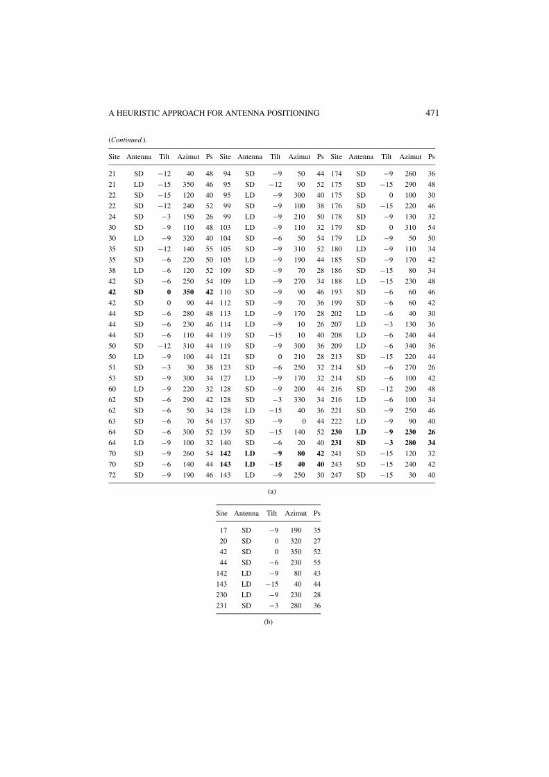
Appendix 4: TS output for highway network with 99% coverage (a) and modified BS bypost optimization with 100% coverage (b)
Site Antenna Tilt Azimut Ps Site Antenna Tilt Azimut Ps Site Antenna Tilt Azimut Ps
9 SD −12 160 46 74 SD −6 210 28 144 LD −9 10 34
9 SD −6 40 36 74 SD −3 350 42 144 LD −3 150 30
13 SD 0 220 30 78 LD −6 300 28 145 LD −9 330 40
14 SD −15 160 36 79 SD −6 110 54 148 SD −15 290 42
14 SD −9 20 44 83 SD −3 230 42 148 LD −6 90 42
17 SD −9 190 34 87 LD −9 320 44 149 SD −6 60 54
17 SD −9 0 42 88 SD −6 290 26 154 LD −6 260 46
18 LD 0 10 34 89 SD −3 290 50 156 SD 0 40 46
20 SD −9 20 30 92 SD −12 250 54 165 LD −6 230 34
20 SD 0 320 26 93 LD −9 310 44 172 LD 0 290 42
(Continued on next page.)
A HEURISTIC APPROACH FOR ANTENNA POSITIONING 471
(Continued ).
Site Antenna Tilt Azimut Ps Site Antenna Tilt Azimut Ps Site Antenna Tilt Azimut Ps
21 SD −12 40 48 94 SD −9 50 44 174 SD −9 260 36
21 LD −15 350 46 95 SD −12 90 52 175 SD −15 290 48
22 SD −15 120 40 95 LD −9 300 40 175 SD 0 100 30
22 SD −12 240 52 99 SD −9 100 38 176 SD −15 220 46
24 SD −3 150 26 99 LD −9 210 50 178 SD −9 130 32
30 SD −9 110 48 103 LD −9 110 32 179 SD 0 310 54
30 LD −9 320 40 104 SD −6 50 54 179 LD −9 50 50
35 SD −12 140 55 105 SD −9 310 52 180 LD −9 110 34
35 SD −6 220 50 105 LD −9 190 44 185 SD −9 170 42
38 LD −6 120 52 109 SD −9 70 28 186 SD −15 80 34
42 SD −6 250 54 109 LD −9 270 34 188 LD −15 230 48
42 SD 0 350 42 110 SD −9 90 46 193 SD −6 60 46
42 SD 0 90 44 112 SD −9 70 36 199 SD −6 60 42
44 SD −6 280 48 113 LD −9 170 28 202 LD −6 40 30
44 SD −6 230 46 114 LD −9 10 26 207 LD −3 130 36
44 SD −6 110 44 119 SD −15 10 40 208 LD −6 240 44
50 SD −12 310 44 119 SD −9 300 36 209 LD −6 340 36
50 LD −9 100 44 121 SD 0 210 28 213 SD −15 220 44
51 SD −3 30 38 123 SD −6 250 32 214 SD −6 270 26
53 SD −9 300 34 127 LD −9 170 32 214 SD −6 100 42
60 LD −9 220 32 128 SD −9 200 44 216 SD −12 290 48
62 SD −6 290 42 128 SD −3 330 34 216 LD −6 100 34
62 SD −6 50 34 128 LD −15 40 36 221 SD −9 250 46
63 SD −6 70 54 137 SD −9 0 44 222 LD −9 90 40
64 SD −6 300 52 139 SD −15 140 52 230 LD −9 230 26
64 LD −9 100 32 140 SD −6 20 40 231 SD −3 280 34
70 SD −9 260 54 142 LD −9 80 42 241 SD −15 120 32
70 SD −6 140 44 143 LD −15 40 40 243 SD −15 240 42
72 SD −9 190 46 143 LD −9 250 30 247 SD −15 30 40
(a)
Site Antenna Tilt Azimut Ps
17 SD −9 190 35
20 SD 0 320 27
42 SD 0 350 52
44 SD −6 230 55
142 LD −9 80 43
143 LD −15 40 44
230 LD −9 230 28
231 SD −3 280 36
(b)

472 VASQUEZ AND HAO
Notes
1. The formal definition of the notion of cell is given later in Section 3.1.2. The choice, done in Reininger (1997) and Reininger and Caminada (1998a), is based on the fact that each point
STP has 8 neighboring STP.3. Notice that non-uniformed costs have no incidence for the heuristic approach presented in this paper.
References
Ballard, D.H. and C.M. Brown. (1982). Computer Vision. Englewood Cliffs, NJ: Prentice Hall.Box, F. (1978). “A Heuristic Technique for Assigning Frequency to Mobile Radio Nets.” IEEE Transactions on
Vehicular Technology 27(2), 57–64.Calegari, P., F. Guidec, P. Kuonen, B. Chamaret, S. Ubeda, S. Josselin, D. Agner, and M. Pizarosso. (1996).
“Radio Network Planning with Combinatorial Optimisation Algorithms.” ACTS Mobile Communications May,707–713.
Crompton, W., S. Hurley, and N.M. Stephen. (1994). “A Parallel Genetic Algorithm for Frequency AssignmentProblems.” In Proc. of IMACS SPRANN’94, pp. 81–84.
Duque-Anton, M., D. Kunz, and B. Ruber. (1993). “Channel Assignment for Cellular Radio Using SimulatedAnnealing.” IEEE Transactions on Vehicular Technology 42, 14–21.
Fortune, S.J., D.M. Gay, B.W. Kernighan, O. Landron, R.A. Valenzuela, and M.H. Wright. (1995). “WISE De-sign of Indoor Wireless Systems: Practical Computation and Optimization.” IEEE Computational Science &Engineering, Spring 1995, pp. 58–68.
Funabiki, N. and Y. Takefuji. (1992). “A Neural Network Parallel Algorithm for Channel Assignment Problemsin Cellular Radio Network.” IEEE Transactions on Vehicular Technology 41, 430–437.
Glover, F. and M. Laguna. (1997). Tabu Search. Dordrecht, The Netherlands: Kluwer Academic Publishers.Hao, J.K. and R. Dorne. (1995). “Study of Genetic Search for the Frequency Assignment Problem.” Lecture Notes
in Computer Science. Artificial Evolution 95, Berlin: Springer-Verlag, Vol. 1063, pp. 333–344.Hao, J.K., R. Dorne, and P. Galinier. (1998). “Tabu Search for Frequency Assignment in Mobile Radio Networks.”
Journal of Heuristics 4(1), 47–62.Hurley, S., S.U. Thiel, and D.H. Smith. (1996). “A Comparison of Local Search Algorithms for Radio Link Fre-
quency Assignment Problems.” In Proc. of ACM Symposium on Applied Computing, Philadelphia, pp. 251–257.Jaumard, B., O. Marcotte, C. Meyer, and T. Vovor: “Comparison of Column Generation Models for Channel
Assignment in Cellular Networks.” Discrete Applied Mathematics (to appear).Lai, W.K. and G. Coghill. (1996). “Channel Assignment Through Evolutionary Optimization.” IEEE Transaction
on Vehicular Technology 45(1), 91–95.McGeehan, J.P. and H.R. Anderson. (1994). “Optimizing Microcell Base Station Locations Using Simulated
Annealing Techniques.” In Proc. of the IEEE Vehicular Technology Conference, pp. 858–862.Molina, A., G.E. Athanasiadou, and A.R. Nix. (1999). “The Automatic Location of Base-Stations for Optimised
Cellular Coverage: A new Combinatorial Approach.” IEEE Vehicular Technologies Conference, Houston, Spring1999.
Reininger, P. (1997). “ARNO Radio Network Optimisation Problem Modelling,” ARNO Deliverable N 1-A 1-Part1. FT. CNET, July 15, 1997.
Reininger, P. and A. Caminada. (1998a). “Model for GSM Radio Network Optimisation.” In 2nd Intl. ACM/IEEEMobicom Workshop on Discrete Algorithms and Methods for Mobile Computing and Communications (DIALM),Dallas, December 16, 1998.
Reininger, P. and A. Caminada. (1998b). “Connectivity Management on Mobile Network Design.” In Proc. of the10th Conference of the European Consortium for Mathematics in Industry, June 1998.
Sherali, H.D., C.M. Pendyala, and T.S. Rappaport. (1996). “Optimal Location of Transmitters for Micro-CellularRadio Communication System Design.” IEEE Journal on Selected Areas in Communications 14(4), 662–673.