a tabu search heuristic for multi-period clustering to
TRANSCRIPT
Wright State University Wright State University
CORE Scholar CORE Scholar
Browse all Theses and Dissertations Theses and Dissertations
2008
A Tabu Search Heuristic for Multi-Period Clustering to Rationalize A Tabu Search Heuristic for Multi-Period Clustering to Rationalize
Delivery Operations Delivery Operations
Surya Sudha Khambhampati Wright State University
Follow this and additional works at: https://corescholar.libraries.wright.edu/etd_all
Part of the Operations Research, Systems Engineering and Industrial Engineering Commons
Repository Citation Repository Citation Khambhampati, Surya Sudha, "A Tabu Search Heuristic for Multi-Period Clustering to Rationalize Delivery Operations" (2008). Browse all Theses and Dissertations. 823. https://corescholar.libraries.wright.edu/etd_all/823
This Thesis is brought to you for free and open access by the Theses and Dissertations at CORE Scholar. It has been accepted for inclusion in Browse all Theses and Dissertations by an authorized administrator of CORE Scholar. For more information, please contact [email protected].
A Tabu Search Heuristic for Multi-PeriodClustering to Rationalize Delivery Operations
A thesis submitted in partial fulfillmentof the requirements for the degree of
Master of Science in Engineering
by
Surya Sudha KhambhampatiB.Tech., Nagarjuna University, 2004
2008Wright State University
Wright State UniversitySCHOOL OF GRADUATE STUDIES
May 14, 2005
I HEREBY RECOMMEND THAT THE THESIS PREPARED UNDER MY SUPER-VISION BY Surya Sudha Khambhampati ENTITLED A Tabu Search Heuristic forMulti-Period Clustering to Rationalize Delivery OperationsBE ACCEPTED IN PARTIALFULFILLMENT OF THE REQUIREMENTS FOR THE DEGREE OFMaster of Science in Engineering .
Xunhui Zhang, Ph.D.Dissertation Director
S. Narayanan, Ph.D., P.E.Department Chair
Committee onFinal Examination
Xinhui Zhang, Ph.D.
Raymond R. Hill, Ph.D.
Frank W. Ciarallo, Ph.D.
Joseph F. Thomas, Jr. , Ph.D.Dean, School of Graduate Studies

COPYRIGHT BY
Surya Sudha Khambhampati
2008
ABSTRACT
Khambhampati, Surya Sudha . M.S. Eng., Department of Biomedical, Industrial and Human Fac-tors Engineering, Wright State University, 2008 .A Tabu Search Heuristic for Multi-Period Clus-tering to Rationalize Delivery Operations.
Delivery operations use centralized warehouses to serve geographically distributed customers.
Resources (e.g. personnel, trucks, stock, equipment) are scheduledfrom the warehouses to dis-
tributed locations with the aim of: (a) meeting customer demands and, (b) rationalizing delivery
operation costs. This thesis investigates the problem of clustering customersbased on their geo-
graphical vicinity and their multi-period demands, while optimally scheduling resources. The prob-
lem is addressed with-and-without capacity constraints of vehicles at the warehouse. This problem
is proven to be NP-Hard. Hence, solutions using state-of-the-art exact methods such as branch and
bound are not pertinent due to the computation complexity involved. In this thesis, we develop a
K-means clustering algorithmfor the initial solution and atabu search heuristicthat combines three
advanced neighborhood search algorithms: (i) shift move, (ii) shift movewith supernodes, and (iii)
ejection chain with supernodes, to accelerate convergence. Using extensive simulations for a vari-
ety of multi-period customer demand instances, we demonstrate that using K-means clustering is an
effective strategy for initial solution in the tabu search method. Also, we show that our shift move
with supernodes algorithm produces notable time savings in comparison with standard neighbor-
hood search algorithms such as shift move, when capacity constraints arenot considered. Further,
when capacity constraints are considered, our ejection chain with supernodes algorithm produces
best solutions for cases where solutions using shift move algorithm are infeasible. For feasible cases
using the shift moves algorithm, significant cost savings are obtained usingthe ejection chain with
supernodes algorithm at the expense of added computation time.
iv
Contents
1 Introduction 1
1.1 Motivation and Significance . . . . . . . . . . . . . . . . . . . . . . . . . . . . . 1
1.1.1 Clustering Customers . . . . . . . . . . . . . . . . . . . . . . . . . . . . . 1
1.1.2 Multi-period Clustering Problem . . . . . . . . . . . . . . . . . . . . . . . 2
1.1.3 Our Proposed Solution . . . . . . . . . . . . . . . . . . . . . . . . . . . . 2
1.2 Thesis Outline . . . . . . . . . . . . . . . . . . . . . . . . . . . . . . . . . . . . . 3
2 Related Work 4
3 Multi-period Clustering Algorithms 7
3.1 Problem Description and Terminology . . . . . . . . . . . . . . . . . . . . . . . .7
3.2 Tabu Search Algorithm . . . . . . . . . . . . . . . . . . . . . . . . . . . . . . . . 9
3.2.1 Neighborhood Search Strategies without Capacity Constraints . . . . .. . 10
3.2.2 Neighborhood Search Strategies with Capacity Constraints . . . . . . . .. 21
4 Performance Evaluation 33
4.0.3 Evaluation Methodology . . . . . . . . . . . . . . . . . . . . . . . . . . . 33
4.0.4 Results Without Capacity Constraints . . . . . . . . . . . . . . . . . . . . 34
4.0.5 Results With Capacity Constraints . . . . . . . . . . . . . . . . . . . . . . 40
5 Conclusions and Future Work 46
Bibliography 48
v
List of Figures
3.1 K-means clustering algorithm illustration example - (a) Customers assigned toclos-
est clusters by Algorithm 1, (b) Recomputed cluster centroids, (c) Customer reas-
signments to their closest cluster centroids, (d) Stationary cluster centroidsupon
repeated customer reassignments . . . . . . . . . . . . . . . . . . . . . . . . . . 15
3.2 Shift with supernode algorithm illustration example - (a) Grouping customers into
supernodes using Algorithm 3, (b) Grouping customers into supernodesbased on
vicinity threshold, (c) Final supernodes of customers within a cluster, (d)Shift of
supernodes between clusters . . . . . . . . . . . . . . . . . . . . . . . . . . . . .20
3.3 Customer grouping into clusters by: (a) K-means clustering algorithm without con-
sidering capacity constraints, (b) Modified K-means clustering algorithm withca-
pacity constraints . . . . . . . . . . . . . . . . . . . . . . . . . . . . . . . . . . . 21
3.4 Length 2 Ejection chain algorithm illustration example - (a) Ejection of supernode
from cluster 4, (b) Eject move triggered in cluster 3 to form reference structure,
(c) Eject move triggered in cluster 1 to form reference structure, (d) Trail move of
ejected supernode from cluster 4 into cluster 2 . . . . . . . . . . . . . . . . . . .25
vi
List of Tables
4.1 Results without capacity constraints for instances with 50 customers . . . .. . . . 37
4.2 Results without capacity constraints for instances with 100 customers . . .. . . . 38
4.3 Results without capacity constraints for instances with 200 customers . . .. . . . 39
4.4 Results with capacity constraints for instances with 50 customers . . . . . . .. . . 43
4.5 Results with capacity constraints for instances with 100 customers . . . . . .. . . 44
4.6 Results with capacity constraints for instances with 200 customers . . . . . .. . . 45
vii

Acknowledgement
I am extremely thankful to Dr. Xinhui Zhang for giving me the opportunity to conduct research
under his supervision. He has guided me all through my research by pointing my efforts in the right
direction, and giving me the freedom to explore different research strategies. I am grateful for his
consent to conduct my research remotely that allowed me to be with my Columbus-based family.
He boosted my confidence in being able to perform my tasks by lauding me on good work and
giving critical reviews in areas where I could improve. I also express my gratitude to Dr. Raymond
R. Hill and Dr. Frank Ciarallo for reviewing my thesis and for being a part of my thesis committee.
I am thankful to my husband Dr. Prasad Calyam for all his support and guidance throughout my
graduate studies. He was the one to encourage me to pursue my Master’s degree. His inspiration
and affection helped me overcome challenging moments in my graduate school experience.
Finally, I would like to take the opportunity to thank my parents Mrs. Bhavani and Mr. Sarma
Kambhampati for all their love and moral support. I also would like to thank my grandfather Mr.
Sankara Narayana Akella and grandmother Mrs. Subbalakshmi Akella who always encouraged my
decision to pursue graduate school. I also would like to thank my sister ArunaKambhampati and
brother Sundeep Kambhamapti for their love and humor.
viii

Dedicated to:
My husband and my parents
ix
Chapter 1
Introduction
1.1 Motivation and Significance
1.1.1 Clustering Customers
Clustering geographically distributed customers is an important step in planningdelivery operations
for a wide variety of applications such as waste management, school bus routing, and postal service
dispatch. The scheduling of resources (e.g. personnel, trucks, stock, equipment) to satisfy customer
demands is challenging for two reasons: (a) customer demands are multi-period in nature i.e., they
vary over different time scales (e.g. days, weeks), (b) resources at central warehouses are limited
and expensive, and hence need to be efficiently used over a finite planning horizon.
Clustering customers while scheduling resources is an intuitive strategy forrationalization of
operation costs. However, the clustering needs to account for: (i) available resource allocation
that may or may not be limited by capacity constraints, and (ii) delivery route selection decisions
that significantly impact delivery operation costs. Similar challenges that involve scheduling based
on multi-period clustering occur in practice in other domains as well. Examples ofsuch domains
include cellular-manufacturing design of electronic circuits and product marketing.
1
1.1.2 Multi-period Clustering Problem
Although the problem of multi-period clustering is relevant in several domains, it is still a hard
combinational optimization problem to solve. Further, there are limited exact methods such as
branch and bound, and column generation to solve this problem. The problem can be summarized
as follows: Given a graphG(N, E) where a set ofN customers have inter-customer edge-setE
with edge-weights or inter-customer distances (we, e ∈ E), partition graphG into L subgraphs or
clusters such that: (a) the inter-cluster edge-weights are maximized, (b) thesum of the edge-weights
in every cluster is minimized, and (c) the sum of customer demands assigned to asingle cluster over
a multi-period do not exceed vehicle capacityQ. Depending on the application, the vehicles in fleet
L may or may not have any capacity constraints. If a capacity constaint is specified, then all the
vehicles in fleetL have equal capacityQ.
1.1.3 Our Proposed Solution
We solve the multi-period clustering problem using two steps. The first step involves forming an ini-
tial solution using theK-means clustering algorithm, which is a standard algorithm used for cluster-
ing data points given by their cartesian co-ordinates(x, y) in linear space. The K-means clustering
algorithm partitions the data points intoL clusters with an objective of maximizing the inter-cluster
distance and minimizing the distance between the data points within each cluster. Since the tradi-
tional K-means clustering algorithm does not address capacity constraints, we propose a modified
K-means clustering algorithm for initial solution formation if capacity constraintsare considered.
The second step involves accelerating convergence of the initial solution with-or-without consid-
ering capacity constraints. For the case where capacity constraint is notconsidered, we develop a
tabu search heuristicthat involves an advanced neighborhood search algorithm calledshift moves
with supernodes. For the case where the capacity constraint is considered, we develop atabu search
heuristic that involves an advanced neighborhood search algorithm called ejection chain with su-
pernodes. We evaluate the performance of our proposed algorithms using extensive simulations for
2
a variety of multi-period customer demand instances given in (Boudia, Louly,et. al., 2007).
1.2 Thesis Outline
The rest of this thesis is organized as follows: Chapter 2 summarizes the related work. Chapter
3 formally describes the research problem, its mathematical models and solution characteristics.
Further, it presents the K-means clustering algorithm for initial solution construction and the tabu
search heuristic with advanced neighborhood search algorithms for bothwith-and-without capacity
constraint cases. Performance results obtained through extensive simulations of our algorithms are
presented in Chapter 4. Finally, Chapter 5 concludes the thesis and presents directions for future
work.
3
Chapter 2
Related Work
The NP-hard (Garey and Johnson, 1979) multi-period clustering problem can be solved using Exact
methods such as the branch and bound (Al-Sultan and Khan, 1996) (Mourgaya and Vanderbeck,
2006). However, such exact methods need strict formulation for construction of tight bounds to be
computationally efficient. Strict formulation refers to specifying all the constraints and objective
function apriori. Also, their computation overheads are prohibitively largefor practical problems
that have several real-time constraints. Further, the exact methods require linear programming of
integer program models that have been proven to give an extremely weak bound of 0 (Brunner et.
al, 2008).
Heuristic methods such as greedy heuristics, genetic algorithm, simulated annealing, ant colony
optimization, and tabu search algorithm can be used to obtain good solutions to the NP-hard multi-
period clustering problem. Amongst these heuristic methods, we choose the tabu search heuristic
because the other methods generally have relatively higher dependenceon initial parameter settings.
The tabu search heuristic has been extensively applied to solve the vehiclerouting problem (VRP) in
works such as (Osman, 1993) (Clarke and Wright, 1964) (Taillard, 1993) (Barbarosoglu and Ozgur,
1999) (Gendreau, et. al., 1994) (Kelly and Xu, 1999). The classical VRP defined in (Osman, 1993)
involves finding efficient routes for vehicles that originate and terminate ata central warehouse
while serving a set of customers under vehicle capacity and total route length constraints. Our
4
problem is similar to the classical VRP in the sense that we cluster customers into different routes.
However, our problem differs from the classical VRP because we do not consider the constraint of
minimizing the route length. Our focus is to mainly satisfy the multi-period demands of customers.
Our solution addresses both the cases where the vehicle capacity constraints may or may not be an
issue. We note that our customer clustering strategy is similar to the approach used in (Sung and Jin,
2000). Here, a set of customers are grouped into clusters such that theeuclidean distance between
each customer and center of its belonging cluster for every such alloactedcustomer is minimized.
Our problem can also be compared to the Generalized Assigment Problem (GAP), which is
defined in (Yagiura, et. al., 1998). The problem involves assigning a setof jobs to a set of agents,
each having a restricted capacity. The goal is to obtain minimum cost assignment of jobs such that
each job is assigned to only a single agent and the available capacity of that agent is not exceeded.
Our problem is similar to GAP in the sense that we have to assign customers to clusters served by
vehicles with capacity limitations. However, we consider assignment of customers based on their
demands over multiple time periods, which is not addressed in GAP. The Generalized Quadratic
Assignment Problem (QGAP) (Cordeau, et. al, 2006) is an extension of theGAP problem. The
goal in QGAP is to assign a set of weighted facilities to a set of capacitated sitessuch that the sum
of assignment and traffic costs is minimized. Further, the total weight of all thefacilities assigned
to the same site should not exceed the site capacity. Our problem is differentfrom QGAP in the
sense that we do not have the traffic cost constraints and our clusteringconsiders customer demands
over multiple time periods. The tabu search heuristic with neighborhood search algorithms has been
applied to solve the GAP and QGAP in works such as (Yagiura and Ibaraki,2004) (Yagiura, et. al.,
1998) (Yagiura, et. al, 1999) (Yagiura, et. al, 1996) (Diaz and Fernandez, 2001).
The neighborhood search algorithms used in our tabu search heuristic can be compared to the
algorithms in earlier works. For instance, our algorithm uses the (Osman, 1993) strategy to insert or
interchange a setλ of customers between clusters. While applying the tabu search heuristic, earlier
works consider different procedures to generate the initial solution. Inour work, our initial solution
is based on the K-means clustering algorithm (Queen, 1967). The K-meansclustering problem is
5
used by (Cano, et. al., 2002) in a GRASP approach to solve the clustering problem without capacity
constraints. They construct multiple solutions using the GRASP algorithm and locally optimize the
solutions using the K-means algorithm.
While considering capacity constraints, we enhance the K-means clusteringalgorithm, and de-
velop an ejection chain algorithm that is based on the algorithm proposed in (Yagiura and Ibaraki,
2004) to solve the GAP. Our problem of dealing with capacity constraints canbe compared to the
popular capacitated clustering problem (CCP) (Franca, et. al., 1999) (Ahmadi and Osman, 2005)
(Scheuerer and Wendolsky, 2006) (Liu, Pu, et. al., 2007). In (Franca, et. al., 1999), a tabu search
heuristic is used to solve the CCP. The initial solution construction involves a sequential method of
clustering. The neighborhood search involves pair wise shift and swapmove and adaptive adjust-
ment of tabu tenure. In (Ahmadi and Osman, 2005), multiple restart approach of the GRASP heuris-
tic is combined with memory structures used in adaptive memory programming (Glover, 1997).
Specifically, memory structures called “elite lists” are maintained to keep track ofbest solutions
and, shift and swap move neighborhoods with single interchanges are used. In (Scheuerer and Wen-
dolsky, 2006), a scatter search heuristic maintains a list of solutions called the “reference set” and
then using path relinking, builds new solutions by combining solutions from the reference set. In
(Liu, Pu, et. al., 2007), a hybrid genetic algorithm approach is used to solve the CCP. This algo-
rithm uses a mutation operator to partition densely populated clusters and mergesparsely populated
clusters. Finally, we use the concept of ‘supernodes’ in Section 4, which is similar to the concept
of cohesive locations used in (Cordeau, et. al, 2006) for solving the QGAP. Cohesive locations
refer to those locations in which a group of customers close to each other are aggregated to form
a single customer location, which is subsequently used in move operations to insert or interchange
customers between clusters.
6
Chapter 3
Multi-period Clustering Algorithms
3.1 Problem Description and Terminology
The multi-period clustering problem can be formally described as follows: Weare given a graph
G(N, E) where a set ofN geographically-dispersed customers have inter-customer edge-setE with
edge-weights or inter-customer distances (we, e ∈ E). The customers require service from a central
warehouse over a planning horizon ofT periods. Each customeri has a fixed non-negative demand
Dit on dayt of the planning horizon that must be satisfied i.e., no shortages are allowed.
The graphG must be partitioned intoL clusters such that a feasible production and delivery
plan can be constructed that takes into account daily demands at the customer sites, while at the
same time rationalizing delivery operations. For this, the clustering should: (a) maximize the inter-
cluster edge-weights, (b) minimize the sum of the edge-weights in every cluster, and (c) not exceed
vehicle capacityQ when the customer demands assigned to a single cluster over a multi-period are
summed. Note that, depending on the application, the vehicles in fleetL may or may not have any
capacity constraints. If a capacity constaint is specified, then all the vehicles in fleetL have equal
capacityQ.
This multi-period clustering problem can be modeled as an integer program. The notations and
the model are as follows:
7
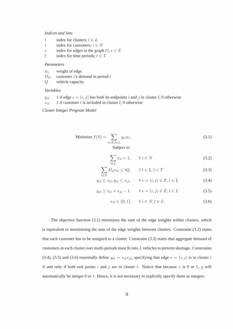
Indices and Sets
l index for clusters;l ∈ Li index for customers;i ∈ Ne index for edges in the graphG, e ∈ Et index for time periods;t ∈ T
Parameters
we weight of edgeDit customeri’s demand in periodtQ vehicle capacity
Variables
yel 1 if edgee = (i, j) has both its endpointsi andj in clusterl; 0 otherwisexil 1 if customeri is included in clusterl; 0 otherwise
Cluster Integer Program Model
Minimize f(S) =∑
e∈E,l∈L
yelwe (3.1)
Subject to
∑
l∈L
xil = 1, ∀ i ∈ N (3.2)
∑
i∈N
Ditxil ≤ tQ, ∀ l ∈ L, t ∈ T (3.3)
yel ≤ xil, yel ≤ xjl, ∀ e = (i, j) ∈ E, l ∈ L (3.4)
yel ≥ xil + xjl − 1, ∀ e = (i, j) ∈ E, l ∈ L (3.5)
xil ∈ {0, 1} ∀ i ∈ N, l ∈ L (3.6)
The objective function (3.1) minimizes the sum of the edge weights within clusters, which
is equivalent to maximizing the sum of the edge weights between clusters. Constraint (3.2) states
that each customer has to be assigned to a cluster. Constraint (3.3) states that aggregate demand of
customers in each cluster over multi-periods must fit intoL vehicles to prevent shortage. Constraints
(3.4), (3.5) and (3.6) essentially defineyel = xilxjl, specifying that edgee = (i, j) is in clusterl
if and only if both end pointsi and j are in clusterl. Notice that becausex is 0 or 1, y will
automatically be integer 0 or 1. Hence, it is not necessary to explicitly specifythem as integers.
8
3.2 Tabu Search Algorithm
Tabu search is a memory-based ‘meta-heuristic’ framework proposed byGlover in the works (Glover,
1989) and (Glover, 1990). In this framework, problem-specific heuristics can be embedded resulting
in the Tabu search algorithm for the particular problem being addressed.Tabu search is based upon
basic local search methods but has an emphasis of building extensive neighborhoods. With such an
emphasis, it escapes the local optimum traps and attains global optimum solutions. The tabu search
requires beginning with an initial solution, sayS, following which,S is iteratively replaced with a
better solution in the neighborhood, sayN(S), until no better solution is found or until a stopping
criterion is met.
Solution Representation: Any solution to our problem is represented as an arrayS of integers with
a length|N | where,N is the number of customers. The index of the array represents the index of
the customers and the associated integer represents the cluster that the customer belongs to.
In the following subsections, we describe the initial solution and neighborhood search algo-
rithms of tabu search heuristic applied to the multi-period clustering problem. First, we address
the case where no capacity constraints are considered. Next, we consider the case where capacity
constraints exist.
Our general approach in developing the neighborhood search algorithms can be termed as
“aggressive exploration”. It involves performing an exploration of thesearch space through moves
that transition from a current stateSt to a stateSt+1 at iterationt using neighborhoods of solutions
statesN(St). To make the search more efficient, and to avoid exhaustive search of theentire search
space, we use acandidate listthat contains a set of candidates to be examined for the next move.
To prevent revisiting the recent solutions, we declare recent moves astabu for a period of thetabu
tenure, sayϑ iterations, and track them using atabu list. Finally, to broaden the search and quickly
bridge between one feasible region to the other, we use astrategic oscillationcomponent. Using
this component, intermediate infeasible solutions are allowed by penalizing an objective function
according to the degree of infeasibility.
9
3.2.1 Neighborhood Search Strategies without Capacity Constraints
Initial Solution using K-means Clustering Algorithm
Construction of a quality initial solution is important since it aids the computational efficiency of a
neighborhood search process. When capacity constraints are not considered, the multi-period clus-
tering is based on geographic vicinity. For this purpose, we use the K-means clustering algorithm
proposed by MacQueen (Queen, 1967)1. The algorithm iteratively clusters a given set of linear
spaced data intoL clusters such that the squared Euclidean distance between each of the nodes2 and
center of its allocated cluster is minimized. Also, it ensures that the squared Euclidean distances be-
tween each of the nodes and the centroid of their allocated cluster are not greater than the distances
to centroids of the remaining clusters. Thus, it minimizes the inter-cluster distance and maximizes
the intra-cluster distance.
Mathematically, we represent the linear space data as a vectorX = [x1, x2, ...,xn] where each
elementxi represents its linear co-ordinates in the multidimensional space. We partitionX into L
clustersC1, C2, ..., CL. Let nc represent the number of instances that belong to clusterCl andµl
represents the centroid of clusterCl. Our goal is to minimize (3.7) shown below -
L∑
l=1
∑
xi∈Cl
‖xi − µl‖2 (3.7)
where,µl is calculated as shown in (3.8).
µl =∑
xi∈Cl
xi/nc (3.8)
1The K-means clustering algorithm is widely used in many application domains such as data mining,geographical information systems and e-commerce.
2Note that a node refers to a single customer in a cluster and weuse both these terms interchangeably inthe remainder of this paper.
10
Initial Seed Selection: The performance of the K-means clustering algorithm depends on the selec-
tion of the initial seed used for cluster construction. A survey of the different methods to generate
the initial seeds can be found in works such as (Bursco, 2004) and (Stainley and Bursco, 2007). We
use asequential methodto generate the initial group centroids. In this method, we first compute
the centroid of all the customers. Next, we choose a point that is farthest from this centroid as the
seed. Since the goal of the K-means clustering algorithm is to maximize the intra-cluster distance,
we construct a cluster far away from the centroid where the density of customers is high. Following
this, we assign a set of customers to this seed. Next, we calculate the centroidof the assigned cus-
tomers. The next seed is chosen as the one which is farthest from this centroid. We assign customers
to this next seed. This process continues until there are no unassigned customers, at which point,
we would have generatedL clusters. Now, the centroids of each of theL clusters are computed and
these centroids become the initial centroids for the K-means clustering algorithm. The algorithm
for sequential cluster construction can be formally described as follows:
11
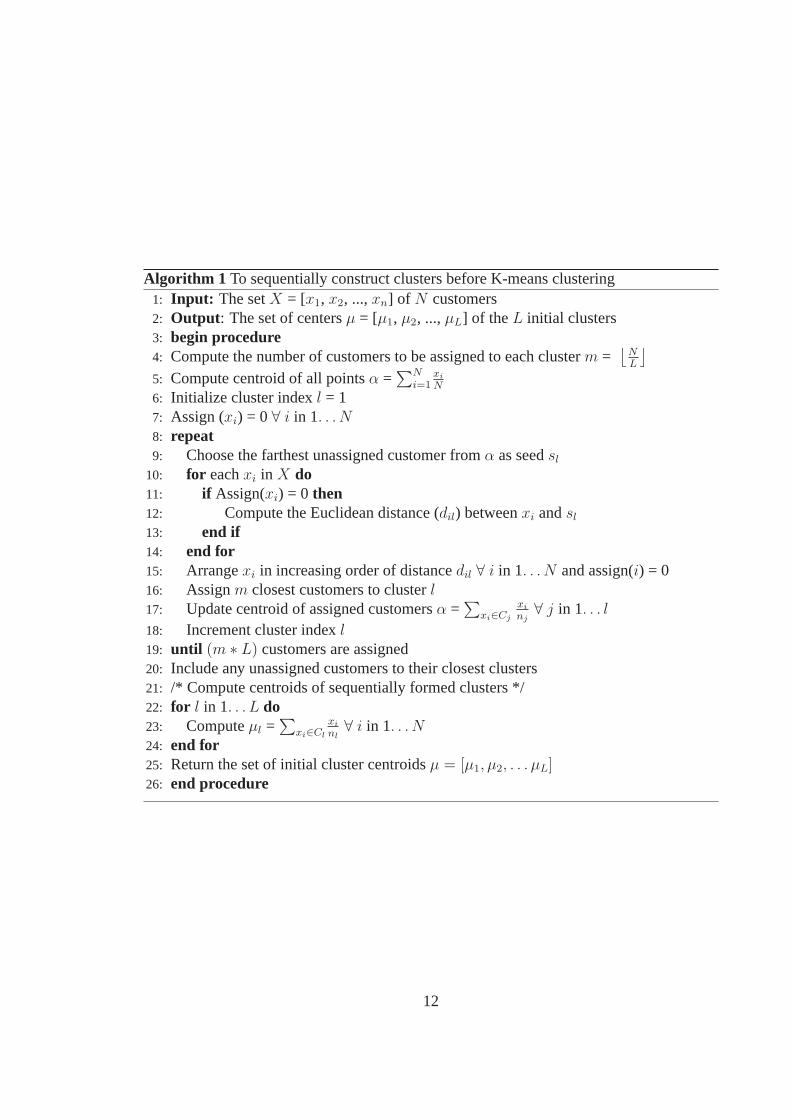
Algorithm 1 To sequentially construct clusters before K-means clustering1: Input: The setX = [x1, x2, ...,xn] of N customers2: Output : The set of centersµ = [µ1, µ2, ...,µL] of theL initial clusters3: begin procedure4: Compute the number of customers to be assigned to each clusterm =
⌊
NL
⌋
5: Compute centroid of all pointsα =∑N
i=1
xi
N
6: Initialize cluster indexl = 17: Assign (xi) = 0 ∀ i in 1. . . N
8: repeat9: Choose the farthest unassigned customer fromα as seedsl
10: for eachxi in X do11: if Assign(xi) = 0 then12: Compute the Euclidean distance (dil) betweenxi andsl
13: end if14: end for15: Arrangexi in increasing order of distancedil ∀ i in 1. . . N and assign(i) = 016: Assignm closest customers to clusterl
17: Update centroid of assigned customersα =∑
xi∈Cj
xi
nj∀ j in 1. . . l
18: Increment cluster indexl19: until (m ∗ L) customers are assigned20: Include any unassigned customers to their closest clusters21: /* Compute centroids of sequentially formed clusters */22: for l in 1. . . L do23: Computeµl =
∑
xi∈Cl
xi
nl∀ i in 1. . . N
24: end for25: Return the set of initial cluster centroidsµ = [µ1, µ2, . . . µL]26: end procedure
12
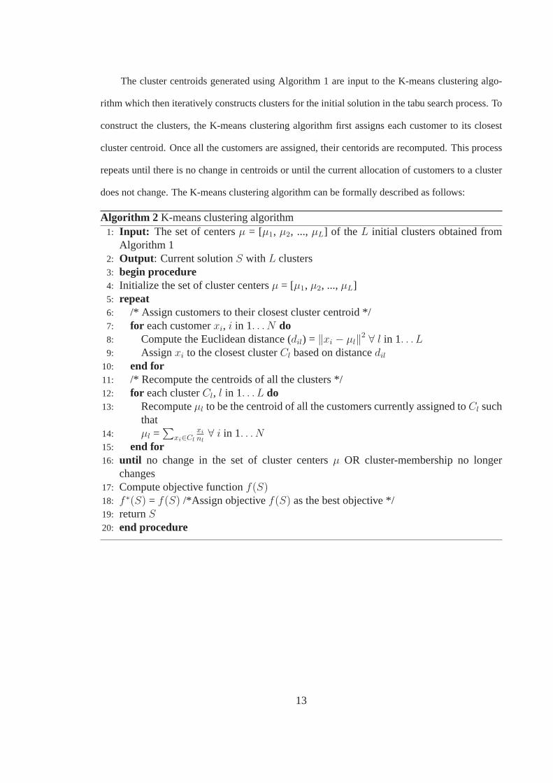
The cluster centroids generated using Algorithm 1 are input to the K-means clustering algo-
rithm which then iteratively constructs clusters for the initial solution in the tabu search process. To
construct the clusters, the K-means clustering algorithm first assigns each customer to its closest
cluster centroid. Once all the customers are assigned, their centorids arerecomputed. This process
repeats until there is no change in centroids or until the current allocation of customers to a cluster
does not change. The K-means clustering algorithm can be formally described as follows:
Algorithm 2 K-means clustering algorithm1: Input: The set of centersµ = [µ1, µ2, ..., µL] of the L initial clusters obtained from
Algorithm 12: Output : Current solutionS with L clusters3: begin procedure4: Initialize the set of cluster centersµ = [µ1, µ2, ...,µL]5: repeat6: /* Assign customers to their closest cluster centroid */7: for each customerxi, i in 1. . . N do8: Compute the Euclidean distance (dil) = ‖xi − µl‖
2 ∀ l in 1. . . L
9: Assignxi to the closest clusterCl based on distancedil
10: end for11: /* Recompute the centroids of all the clusters */12: for each clusterCl, l in 1. . . L do13: Recomputeµl to be the centroid of all the customers currently assigned toCl such
that14: µl =
∑
xi∈Cl
xi
nl∀ i in 1. . . N
15: end for16: until no change in the set of cluster centersµ OR cluster-membership no longer
changes17: Compute objective functionf(S)18: f ∗(S) = f(S) /*Assign objectivef(S) as the best objective */19: returnS
20: end procedure
13
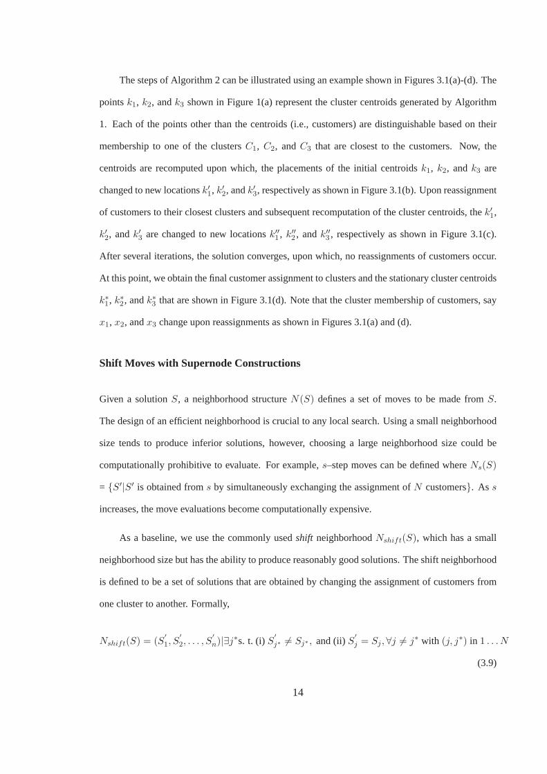
The steps of Algorithm 2 can be illustrated using an example shown in Figures 3.1(a)-(d). The
pointsk1, k2, andk3 shown in Figure 1(a) represent the cluster centroids generated by Algorithm
1. Each of the points other than the centroids (i.e., customers) are distinguishable based on their
membership to one of the clustersC1, C2, andC3 that are closest to the customers. Now, the
centroids are recomputed upon which, the placements of the initial centroidsk1, k2, andk3 are
changed to new locationsk′
1, k′
2, andk′
3, respectively as shown in Figure 3.1(b). Upon reassignment
of customers to their closest clusters and subsequent recomputation of thecluster centroids, thek′
1,
k′
2, andk′
3 are changed to new locationsk′′
1 , k′′
2 , andk′′
3 , respectively as shown in Figure 3.1(c).
After several iterations, the solution converges, upon which, no reassignments of customers occur.
At this point, we obtain the final customer assignment to clusters and the stationary cluster centroids
k∗
1, k∗
2, andk∗
3 that are shown in Figure 3.1(d). Note that the cluster membership of customers, say
x1, x2, andx3 change upon reassignments as shown in Figures 3.1(a) and (d).
Shift Moves with Supernode Constructions
Given a solutionS, a neighborhood structureN(S) defines a set of moves to be made fromS.
The design of an efficient neighborhood is crucial to any local search. Using a small neighborhood
size tends to produce inferior solutions, however, choosing a large neighborhood size could be
computationally prohibitive to evaluate. For example,s–step moves can be defined whereNs(S)
= {S′|S′ is obtained froms by simultaneously exchanging the assignment ofN customers}. As s
increases, the move evaluations become computationally expensive.
As a baseline, we use the commonly usedshift neighborhoodNshift(S), which has a small
neighborhood size but has the ability to produce reasonably good solutions. The shift neighborhood
is defined to be a set of solutions that are obtained by changing the assignment of customers from
one cluster to another. Formally,
Nshift(S) = (S′
1, S′
2, . . . , S′
n)|∃j∗s. t. (i)S′
j∗ 6= Sj∗ , and (ii)S′
j = Sj ,∀j 6= j∗ with (j, j∗) in 1 . . . N
(3.9)
14
Figure 3.1: K-means clustering algorithm illustration example - (a) Customers assignedto closest clusters by Algorithm 1, (b) Recomputed cluster centroids, (c) Customer reas-signments to their closest cluster centroids, (d) Stationary cluster centroids upon repeatedcustomer reassignments
15
We now describe our modified shift move neighborhood search that improves upon the basic
shift move neighborhood search. The motivation for our modification comesfrom the fact that shift
moves are performed between clusters, only one customer at a time. Such anapproach may lead to
multiple shift moves of one or more customers that are likely to be moved to anothercluster based
on their close vicinity. By combining such likely customers into a “supernode” within a cluster,
only one shift move of the supernode is sufficient to obtain the same result obtained using multiple
shift moves.
For each clusterCl with l in 1 . . .L, there could bem supernodes. LetSNj = {SNj1, SNj2,
. . . , SNjm} be the supernode representation of customers that belong to clusterCl. Let αlq and
NClq denote the centroid number of customers in supernodeSNlq, respectively. The supernodes
{SNj1, SNj2, . . . , SNjm} in the setSNj are constructed sequentially as follows: A random cus-
tomer in a cluster is initially designated as an independent node. For the next customer, the distance
of the customer to the independent node is computed. If this distance is within athresholdvalueψ,
then both the customers are grouped together into a “supernode” and the centroid of the supernode
is computed. Otherwise, the customers remain as independent nodes. Thereafter, the supernode
construction process is repeated to obtain either new supernodes, or larger supernodes with updated
centroids, or independent nodes. If there is a scenario where the distance of a customer to one or
more supernode centroids is withinψ, then the customer is grouped into the supernode that has the
minimal centroid-to-node distance. This process repeats until all the customers that belong to the
cluster are evaluated. The supernode construction algorithm can be formally described as follows:
16
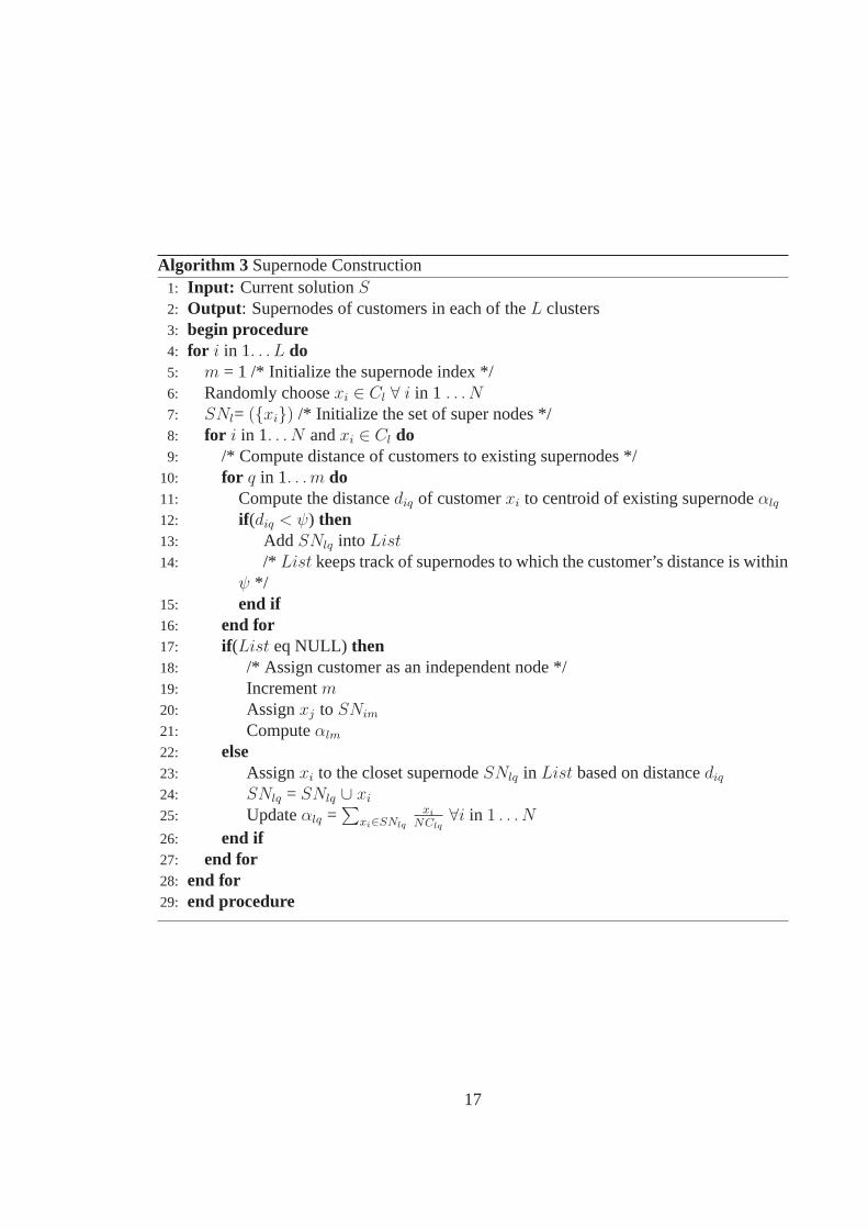
Algorithm 3 Supernode Construction1: Input: Current solutionS2: Output : Supernodes of customers in each of theL clusters3: begin procedure4: for i in 1. . . L do5: m = 1 /* Initialize the supernode index */6: Randomly choosexi ∈ Cl ∀ i in 1 . . . N
7: SNl= ({xi}) /* Initialize the set of super nodes */8: for i in 1. . . N andxi ∈ Cl do9: /* Compute distance of customers to existing supernodes */
10: for q in 1. . . m do11: Compute the distancediq of customerxi to centroid of existing supernodeαlq
12: if (diq < ψ) then13: Add SNlq into List
14: /* List keeps track of supernodes to which the customer’s distance is withinψ */
15: end if16: end for17: if (List eq NULL) then18: /* Assign customer as an independent node */19: Incrementm20: Assignxj to SNim
21: Computeαlm
22: else23: Assignxi to the closet supernodeSNlq in List based on distancediq
24: SNlq = SNlq ∪ xi
25: Updateαlq =∑
xi∈SNlq
xi
NClq∀i in 1 . . . N
26: end if27: end for28: end for29: end procedure
17
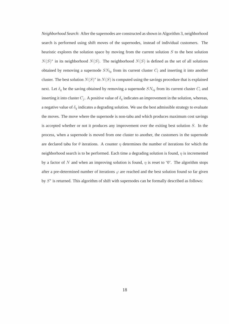
Neighborhood Search: After the supernodes are constructed as shown in Algorithm 3, neighborhood
search is performed using shift moves of the supernodes, instead of individual customers. The
heuristic explores the solution space by moving from the current solutionS to the best solution
N(S)∗ in its neighborhoodN(S). The neighborhoodN(S) is defined as the set of all solutions
obtained by removing a supernodeSNlq from its current clusterCl and inserting it into another
cluster. The best solutionN(S)∗ in N(S) is computed using the savings procedure that is explained
next. Letδq be the saving obtained by removing a supernodeSNiq from its current clusterCi and
inserting it into clusterCj . A positive value ofδq indicates an improvement in the solution, whereas,
a negative value ofδq indicates a degrading solution. We use the best admissible strategy to evaluate
the moves. The move where the supernode is non-tabu and which produces maximum cost savings
is accepted whether or not it produces any improvement over the exiting best solutionS. In the
process, when a supernode is moved from one cluster to another, the customers in the supernode
are declared tabu forθ iterations. A counterη determines the number of iterations for which the
neighborhood search is to be performed. Each time a degrading solution is found,η is incremented
by a factor ofN and when an improving solution is found,η is reset to ‘0’. The algorithm stops
after a pre-determined number of iterationsϕ are reached and the best solution found so far given
by S∗ is returned. This algorithm of shift with supernodes can be formally described as follows:
18
Algorithm 4 Shift with Supernodes1: Input: Initial SolutionS from Algorithm 22: Output : Best SolutionS∗
3: begin procedure4: while (η ≤ ϕ) do5: /* Compute the supernode to be shifted for each cluster */6: for clusterl in 1. . . L do7: Generate supernodes using Algorithm 38: f(N(S)∗) = ∞ /* Initialize the best objective in the neighborhood */9: for q in 1. . . m do
10: /* Remove supernodeSNlq from its current clusterCl with m supernodes */11: dropq =
∑
xi∈SNlqxi ∀i in 1 . . . N
12: Find the best vehiclev to insert intoSNlq
13: /* Compute the cost of this insertion */14: addq =
∑
xi∈Cvxi +
∑
xi∈SNlqxi ∀i in 1 . . . N
15: /* Compute the savingsδq obtained by removal ofSNlq from Cl, and insertioninto Cv */
16: δq = addq - dropq
17: end for18: Compute the supernodeSNlq that obtains maximum cost savings19: δq and customers inSNlq that are non-tabu∀q in 1 . . . m
20: Derive modified solutionNl(S) by removal ofSNlq from Cl and insertion intoCv
21: Computef(Nl(S))22: if (f(Nl(S)) < f(N(S)∗)) then23: N(S)∗ = Nl(S)24: end if25: Accept the best solutionN(S)∗ in the neighborhood26: Set tabu status of customers moved to tabu tenure27: if (f(N(S)∗) < f(S)∗) then28: /* Update the best solution so far */29: S = N(S)∗
30: f(S)∗ = f(N(S)∗)31: S∗ = N(S)∗
32: η = 0 /* Reset the iteration counter */33: else34: S = N(S)∗
35: η = η + N /* Increment the iteration counter */36: end if37: returnf(S)∗
38: end for39: end while40: end procedure
19
Figure 3.2: Shift with supernode algorithm illustration example - (a) Grouping customersinto supernodes using Algorithm 3, (b) Grouping customers into supernodes based onvicinity threshold, (c) Final supernodes of customers within a cluster, (d) Shift of supern-odes between clusters
The steps in Algorithm 3 and Algorithm 4 can be illustrated using an example shown in Fig-
ures 3.2(a)-(d). In Figure 3.2(a), customers relatively closer to eachother in vicinity are grouped
together into supernodes in clusterC4 based on Algorithm 3. This results in clusterC4 having three
supernodesSN41, SN42 andSN43 with centroidsα41, α42, andα43, respectively. In Figure 3.2(b),
customersx4 andx9 are now grouped with the existing supernodes and distances of these two cus-
tomers to the centroidsα41, α42 andα43 are computed. Since the distance ofx4 to supernodeSN42
is within the threshold,x4 is grouped intoSN42. However, the distance ofx9 to centroid of any
of the supernodes is not within the threshold value. Hence,x9 remains as an independent node.
The final construction of the supernodes of customers within clusterC4 are shown in Figure 3.2(c).
After these supernodes are constructed, the shift operation is performed between the clusters. In this
scenario, the supernodeSN41 can be inserted into either clusterC1,C2 or C3. The shift operation
on SN41 results in insertion ofSN41 into clusterC3, which produces an best insertion relative to
the costlyC1 andC2 cluster insertions.
20
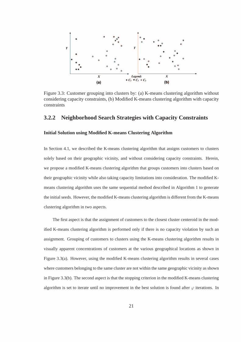
Figure 3.3: Customer grouping into clusters by: (a) K-means clustering algorithm withoutconsidering capacity constraints, (b) Modified K-means clustering algorithm with capacityconstraints
3.2.2 Neighborhood Search Strategies with Capacity Constraints
Initial Solution using Modified K-means Clustering Algorith m
In Section 4.1, we described the K-means clustering algorithm that assigns customers to clusters
solely based on their geographic vicinity, and without considering capacityconstraints. Herein,
we propose a modified K-means clustering algorithm that groups customers into clusters based on
their geographic vicinity while also taking capacity limitations into consideration. The modified K-
means clustering algorithm uses the same sequential method described in Algorithm 1 to generate
the initial seeds. However, the modified K-means clustering algorithm is different from the K-means
clustering algorithm in two aspects.
The first aspect is that the assignment of customers to the closest cluster centeroid in the mod-
ified K-means clustering algorithm is performed only if there is no capacity violation by such an
assignment. Grouping of customers to clusters using the K-means clustering algorithm results in
visually apparent concentrations of customers at the various geographical locations as shown in
Figure 3.3(a). However, using the modified K-means clustering algorithm results in several cases
where customers belonging to the same cluster are not within the same geographic vicinity as shown
in Figure 3.3(b). The second aspect is that the stopping criterion in the modified K-means clustering
algorithm is set to iterate until no improvement in the best solution is found afterϕ iterations. In
21
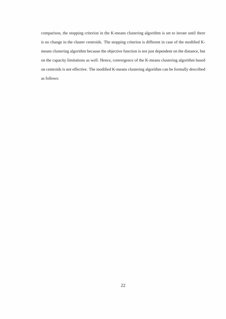
comparison, the stopping criterion in the K-means clustering algorithm is set to iterate until there
is no change in the cluster centroids. The stopping criterion is different in case of the modified K-
means clustering algorithm because the objective function is not just dependent on the distance, but
on the capacity limitations as well. Hence, convergence of the K-means clustering algorithm based
on centroids is not effective. The modified K-means clustering algorithm can be formally described
as follows:
22
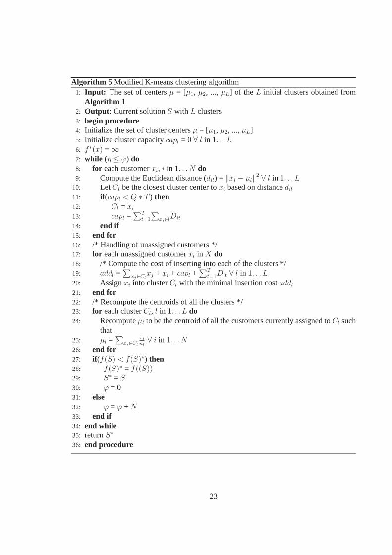
Algorithm 5 Modified K-means clustering algorithm1: Input: The set of centersµ = [µ1, µ2, ..., µL] of the L initial clusters obtained from
Algorithm 12: Output : Current solutionS with L clusters3: begin procedure4: Initialize the set of cluster centersµ = [µ1, µ2, ...,µL]5: Initialize cluster capacitycapl = 0 ∀ l in 1. . . L
6: f ∗(x) = ∞7: while (η ≤ ϕ) do8: for each customerxi, i in 1. . . N do9: Compute the Euclidean distance (dil) = ‖xi − µl‖
2 ∀ l in 1. . . L
10: Let Cl be the closest cluster center toxi based on distancedil
11: if (capl < Q ∗ T ) then12: Cl = xi
13: capl =∑T
t=1
∑
xi∈lDit
14: end if15: end for16: /* Handling of unassigned customers */17: for each unassigned customerxi in X do18: /* Compute the cost of inserting into each of the clusters */19: addl =
∑
xj∈Clxj + xi + capl +
∑T
t=1Dit ∀ l in 1. . . L
20: Assignxi into clusterCl with the minimal insertion costaddl
21: end for22: /* Recompute the centroids of all the clusters */23: for each clusterCl, l in 1. . . L do24: Recomputeµl to be the centroid of all the customers currently assigned toCl such
that25: µl =
∑
xi∈Cl
xi
nl∀ i in 1. . . N
26: end for27: if (f(S) < f(S)∗) then28: f(S)∗ = f((S))29: S∗ = S
30: ϕ = 031: else32: ϕ = ϕ + N
33: end if34: end while35: returnS∗
36: end procedure
23
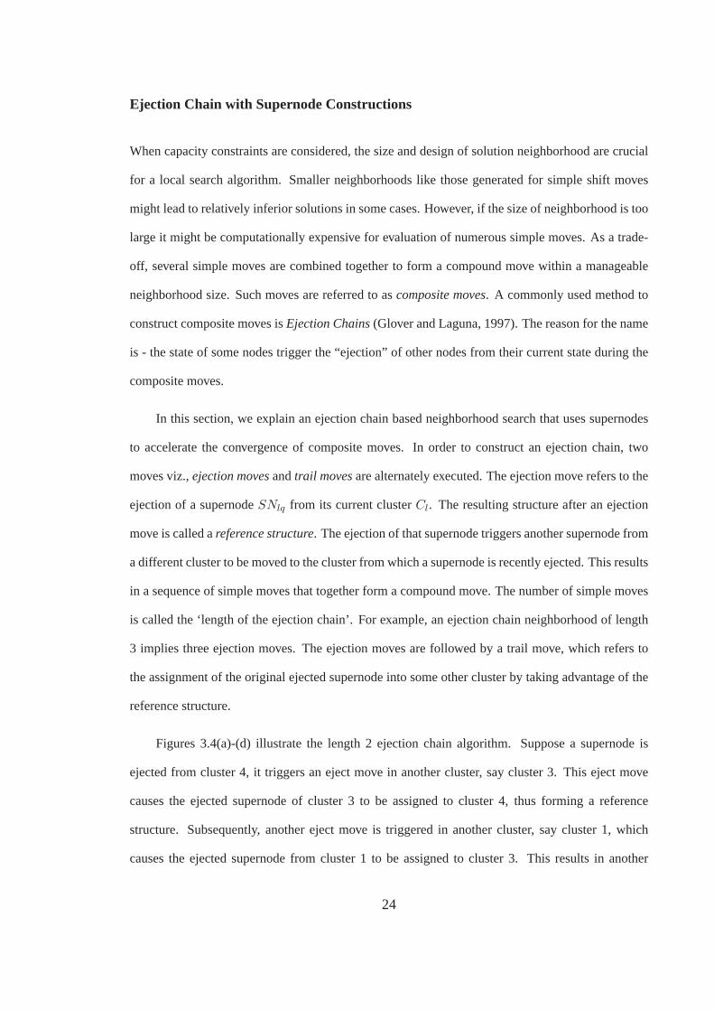
Ejection Chain with Supernode Constructions
When capacity constraints are considered, the size and design of solutionneighborhood are crucial
for a local search algorithm. Smaller neighborhoods like those generated for simple shift moves
might lead to relatively inferior solutions in some cases. However, if the size of neighborhood is too
large it might be computationally expensive for evaluation of numerous simple moves. As a trade-
off, several simple moves are combined together to form a compound move within a manageable
neighborhood size. Such moves are referred to ascomposite moves. A commonly used method to
construct composite moves isEjection Chains(Glover and Laguna, 1997). The reason for the name
is - the state of some nodes trigger the “ejection” of other nodes from their current state during the
composite moves.
In this section, we explain an ejection chain based neighborhood search that uses supernodes
to accelerate the convergence of composite moves. In order to constructan ejection chain, two
moves viz.,ejection movesandtrail movesare alternately executed. The ejection move refers to the
ejection of a supernodeSNlq from its current clusterCl. The resulting structure after an ejection
move is called areference structure. The ejection of that supernode triggers another supernode from
a different cluster to be moved to the cluster from which a supernode is recently ejected. This results
in a sequence of simple moves that together form a compound move. The number of simple moves
is called the ‘length of the ejection chain’. For example, an ejection chain neighborhood of length
3 implies three ejection moves. The ejection moves are followed by a trail move, which refers to
the assignment of the original ejected supernode into some other cluster by taking advantage of the
reference structure.
Figures 3.4(a)-(d) illustrate the length 2 ejection chain algorithm. Suppose a supernode is
ejected from cluster 4, it triggers an eject move in another cluster, say cluster 3. This eject move
causes the ejected supernode of cluster 3 to be assigned to cluster 4, thusforming a reference
structure. Subsequently, another eject move is triggered in another cluster, say cluster 1, which
causes the ejected supernode from cluster 1 to be assigned to cluster 3. This results in another
24
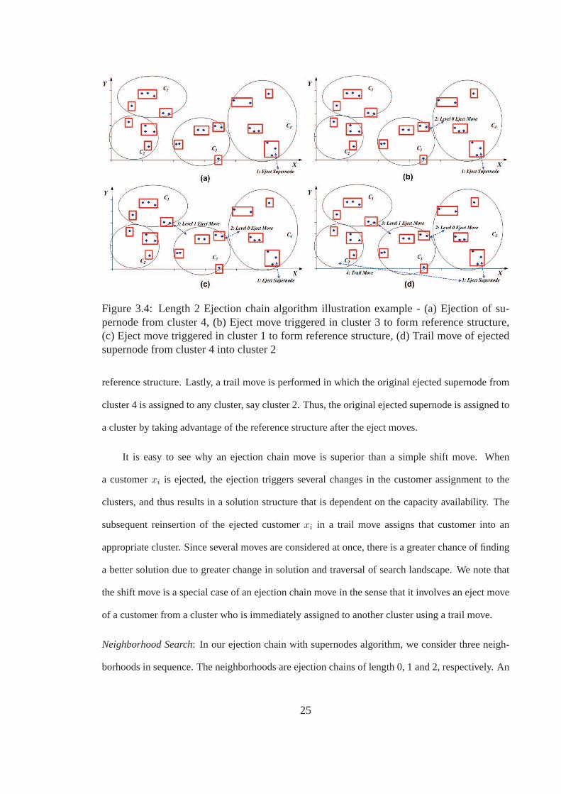
Figure 3.4: Length 2 Ejection chain algorithm illustrationexample - (a) Ejection of su-pernode from cluster 4, (b) Eject move triggered in cluster 3to form reference structure,(c) Eject move triggered in cluster 1 to form reference structure, (d) Trail move of ejectedsupernode from cluster 4 into cluster 2
reference structure. Lastly, a trail move is performed in which the originalejected supernode from
cluster 4 is assigned to any cluster, say cluster 2. Thus, the original ejected supernode is assigned to
a cluster by taking advantage of the reference structure after the eject moves.
It is easy to see why an ejection chain move is superior than a simple shift move.When
a customerxi is ejected, the ejection triggers several changes in the customer assignmentto the
clusters, and thus results in a solution structure that is dependent on the capacity availability. The
subsequent reinsertion of the ejected customerxi in a trail move assigns that customer into an
appropriate cluster. Since several moves are considered at once, there is a greater chance of finding
a better solution due to greater change in solution and traversal of searchlandscape. We note that
the shift move is a special case of an ejection chain move in the sense that it involves an eject move
of a customer from a cluster who is immediately assigned to another cluster usinga trail move.
Neighborhood Search: In our ejection chain with supernodes algorithm, we consider three neigh-
borhoods in sequence. The neighborhoods are ejection chains of length 0, 1 and 2, respectively. An
25
ejection chain of length 0 is a “shift neighborhood”, length 1 is referred toas “double shift neigh-
borhood” and length 2 is referred to as a “long chain neighborhood”. To quickly search from one
feasible region to another, we usestrategic oscillationin our search process that allows searching
into infeasible regions i.e., allows temporary infeasible solutions. However, we penalize the infeasi-
ble solutions based on the degree of infeasibility by adding a penalty factor tothe objective function
as follows:
f ′(x) = f(x) +∑
l∈L,t∈T
β∗plt(x) (3.10)
where
plt = min(0, tQ −∑
i∈N
Ditxil) (3.11)
The parameterβ can be given as a positive constant or can be dynamically changed in each
iteration. If β is large, it penalizes moves across the infeasible region. Ifβ is small, it does not
introduce any penalty effects. The value ofβ is dynamically calculated in each iteration as follows:
Initially, β is set to 100 *NC. If a current solution is feasible for the given capacity constraints,
thenβ is multiplied by 0.5, otherwiseβ is multiplied by 1.5. For more details regarding dynamically
changing theβ parameter, the reader is referred to (Yagiura and Ibaraki, 2004).
During the iterations, we use the best admissible strategy which involves accepting the best
neighborhood amongst shift, double shift and long chain. This ejection chain with supernodes
algorithm iterates until no improvement is found for a thresholdϕ iterations. The generalized
ejection chain with supernodes algorithm can be explained for any length asfollows: We first eject
a supernodeSNlq from its current clusterCl. Consequently, the supernodeSNlq becomes free
and the amount of resources available atCl increase. Given the increased capacity inCl, we shift
another supernode into the cluster from which the first supernode is ejected, thus resulting in an
eject move. This eject move is repeated as determined by the length of the ejection chain. In the
process, a reference structure a.k.a. partial solution is created.
26
Finally, a trail move is performed by inserting the free customers inSNlq to the appropriate
cluster by taking advantage of the reference structure. Since we perform ejection chains with su-
pernodes, several moves are considered at once in every iteration, thus shortening the ejection chain
length.
Our ejection chain with supernodes algorithm has three steps. The first step is called “cost
saving procedure”, which selects a supernode to be ejected. The second step is called “eject move
procedure”, which builds the reference structure by performing ejectmoves in sequence. The final
step is called “trail move procedure”, which constructs a complete solution. In the following, we
describe these three steps in detail:
Cost Saving Procedure: The cost saving procedure uses a candidate list strategy to come up with
the best candidates to be ejected from their respective clusters. Ejection of appropriate candidates
reduces the computation effort as opposed to exhaustive evaluation of the ejection of all customers.
We compute the savingsδq obtained by removing a supernodeSNlq from its current cluster and
inserting it into another cluster. The supernode that produces maximum cost savings would be
considered as a candidate to be ejected. Thus, the cost savings procedure removes a customer that
has a better fit in another cluster rather than its current cluster. After the cost savings procedure
is executed, we obtain a listCList that contains all the candidates to be ejected. The cost saving
procedure can be formally described as follows:
27
Algorithm 6 Cost Savings1: Input: Current SolutionS2: Output : Candidate ListCList
3: begin procedure4: for clusterl in 1. . . L do5: Generate supernodes usingAlgorithm 36: for q in 1. . . m do7: /* Remove supernodeSNlq from its current clusterCl with m supernodes */8: dropq =
∑
xi∈SNlqxi ∀i in 1 . . . N
9: Find the best vehiclev to insert intoSNlq
10: /* Compute the cost of this insertion */11: addq =
∑
xi∈Cvxi +
∑
xi∈SNlqxi ∀i in 1 . . . N
12: /* Compute the savingsδq obtained by removal ofSNlq from Cl and insertion intoCv */
13: δq = addq - dropq
14: end for15: Compute the supernodeSNlq that obtains maximum cost savings16: δq and customers inSNlq that are non-tabu∀q in 1 . . . m
17: best supernode(l) = SNlq
18: best localdelta(l) = δq
19: end for20: Find the supernodeSNlq that has the minimum value ofbest localdelta(l) ∀ l in 1 . . . L
21: CList = {xl ∈ SNlq}22: end procedure
28
Eject Move Procedure: An eject move refers to shifting of a supernode into the cluster from which
a supernode has been recently ejected. The ejection of a supernode from its current clusterCl
increases resource availability in that cluster and hence triggers insertionof another supernode (of
a different cluster) into that cluster. Thus, partial solutions or reference structures are created in
this process. We denote the cluster from which a supernode is ejected asref. When supernodes
from other clusters are considered for insertion intoref, we choose only the supernode whose cost
of insertion intoref is minimal. To prevent the revisiting of solutions, supernodes moved from their
current cluster toref are not moved fromref until the duration of its tabu-tenure. Thus, we only
consider ejection moves of supernodes that are non-tabu. This procedure takes as input the cluster
ref and inserts the best supernode intoref. The clusterCprev to which the best supernode previously
belonged is returned as a reference clusterref for subsequent operations. The eject move procedure
can be formally described as follows:
29
Algorithm 7 Eject Move1: Input: Current SolutionS2: Output : Reference Clusterref3: begin procedure4: prev = ref
5: /* Remove supernodes from their current cluster for insertion intoprev */6: for clusterl in 1. . . L andl <> prev do7: Generate supernodes using Algorithm 38: for q in 1. . . m do9: /* Remove supernodeSNlq from its current clusterCl with m supernodes */
10: dropq =∑
xi∈SNlqxi ∀i in 1 . . . N
11: /* Compute the cost of insertion intoprev */12: addq =
∑
xi∈Cprev,xi∈SNlqxi ∀i in 1 . . . N
13: /* Compute the savingsδq obtained by removal ofSNlq from Cl and insertion intoCprev */
14: δq = addq - dropq
15: end for16: Compute the supernodeSNlq that obtains maximum cost savingsδq and customers
in SNlq
17: that are non-tabu∀q in 1 . . . m, ∀l in 1 . . . L andl <> prev
18: best supernode(l) = SNlq
19: best ref = Cl
20: for i in 1. . . N andxi ∈ best supernode do21: Assignxi to prev
22: Update current solutionS23: tabu eject(xi) = θ
24: end for25: ref = best ref
26: returnref
27: end for28: end procedure
30
Trail Move Procedure: Trail move involves insertion of free candidate supernodes to a cluster which
produces minimal insertion cost. For selecting such a cluster, insertion costof free candidates into
clusters other than the cluster from which the candidates previously belonged is computed. The
cluster that produces the minimal insertion cost for the candidates is selectedfor insertion. After
such trail moves, a complete solution is constructed which takes advantage ofthe intermediate
reference structures obtained from eject moves.
Ejection Chain Algorithm: Recall that the ejection chain algorithm uses the three procedures de-
scribed above. The ejection chain algorithm first ejects a supernode using the cost saving proce-
dure. Then, eject moves are performed for the length of the ejection chain. Finally, a trail move
is performed. Starting from a current solutionS, three neighborhoodsN0(S), N1(S), andN2(S)
are considered. Each of the neighborhoods corresponds to ejection chain of lengths 0, 1 and 2,
respectively. We use a best admissible strategy and move to a best neighborhoodN(S)∗, which has
the least objective function value amongst all these neighborhoods. Thealgorithm iterates until no
improvement in the objective functionf(S) is found forϕ iterations and the best solution found so
far S∗ is returned. The ejection chain algorithm can be formally described as follows:
31
Algorithm 8 Ejection Chain1: Input: Initial SolutionS from Algorithm 5,length of ejection chain2: Output : Best SolutionS∗
3: begin procedure4: while (η ≤ ϕ) do5: level = 06: while (level ≤ length) do7: f(N(S)∗) = ∞ /* Initialize the best objective in the neighborhood */8: CList = supernodeSNlq returned by Algorithm 6 that needs to be ejected9: ref = clusterCl to which theCList customer belongs
10: Nlevel(S) = Modify S by removingCList customers fromref11: /* Perform ejection move for the duration of ejection chain length */12: for j in 1. . . level andlevel 6= 0 do13: /* Construct a reference structure */14: ref next = return value of eject move invoked withref andNlevel(S) inputs15: ref = ref next
16: end for17: Nlevel(S) = Perform trail move onNlevel(S) to construct a complete solution18: Computef(Nlevel(S))19: if (f(Nlevel(S)) < f(N(S)∗)) then20: N(S)∗ = Nlevel(S)21: end if22: end while23: Accept the best solutionN(S)∗ in the neighborhood24: Set tabu status of customers moved to tabu tenure25: if (f(N(S)∗) < f(S)∗) then26: /* Update the best solution so far */27: S = N(S)∗
28: f(S)∗ = f(N(S)∗)29: S∗ = N(S)∗
30: η = 0 /* Reset the iteration counter */31: else32: S = N(S)∗
33: η = η + N /* Increment the iteration counter */34: end if35: returnf(S)∗
36: end while37: end procedure
32
Chapter 4
Performance Evaluation
In this section, we first describe the performance evaluation methodology toevaluate our proposed
algorithms. Next, we present the simulation results of our K-means and shift with supernodes al-
gorithms when compared with the basic shift algorithm without considering capacity constraints.
Finally, we present the simulation results of our modified K-means and ejection chain with su-
pernodes algorithms when compared with the basic shift algorithm, in the presence of capacity
constraints.
4.0.3 Evaluation Methodology
Our proposed algorithms have been implemented and executed using the Xpress-MP development
environment (Guret, et. al, 2002) running on a PC with Windows XP operating system, 1.6 GHz
CPU and 512 MB RAM. For the multi-period customer demands input, we use the instances that
were randomly generated by the authors in (Boudia, Louly, et. al., 2007).These instances are
comprised of three sets of 30 instances with 50, 100, and 200 customers respectively, all with 20
time periodsT . Other inputs such as number of vehiclesL and the vehicle capacityQ, if and
when considered in the implementation, depend on the number of customers. The vehicle capacity
caters to two days of consumption for the full set of customers, when no capacity constraints are
considered. In the case where capacity constraints are considered,Q is calcuated similar to the
33
method suggested in (Boudia, Louly, et. al., 2007) i.e.,Q value is chosen to be less than, but close
to the average demand of all the customers across time periodT .
4.0.4 Results Without Capacity Constraints
Tables 4.1 - 4.3 show the simulation results of the 30 instances of data with 50, 100 and 200 cus-
tomers respectively for three heuristics: (i) basic shift (BS) algorithm, (ii)K-means (KM) algorithm,
and (iii) K-means plus shift with supernodes (KMS) algorithm. For each instance, we show the value
of the objective function, and the run time in seconds. In addition, we show the average cost and
average time across all the customers for the three heuristics. Further, we mark in bold the best
solutions found in the simulation and indicate the total number of best solutions found. We define
the best solution as the one that is cost-wise lesser for a particular instanceamong the BS, KM, and
KMS algorithms.
The number of iterationsϕ for BS algorithm and the KMS algorithm is set toN ∗ 50. Conse-
quently, as the number of customersN increases, the iterations increase correspondingly. The tabu
tenureθ also depends on the number of customers and is set to0.1 ∗ N . For each of the customer
sizes, the thresholdψ for grouping customers into supernodes is dynamically calculated by taking
into account the average of the inter-customer distances in the data set. We choose the value ofψ
such that it decreases with the increase in the number of customers. The reason for this decrease of
ψ is as follows - higher the number of customers, higher are the number of clusters and lesser is the
inter-cluster distance. Due to low inter-cluster distances, customers close toeach other may belong
to two different clusters. Hence, choosing a value ofψ to be small allows for grouping tightly close
customers into supernodes that would then belong to the same cluster.
From Table 4.1 i.e., 50 customers case results, we can note that KMS algorithmproduces the
best solutions in terms of objective function values for 4 customer instances. For the other instances,
it can be observed that BS algorithm and KM algorithm have similar values of objective function.
However, KMS algorithm produces solutions with relatively lesser computation time and with better
34
cost than BS algorithm for all instances. Specifically, there is an averageof 52% in time savings
and 0.4% cost savings when KMS algorithm is used. With reference to KM algorithm, although
its sole purpose is to construct the initial solution, its solutions deviate by an average of only 5%
from the best solutions. Thus, we can conclude that the KM algorithm significantly accelerates the
performance of neighborhood search. We can note that the reduction incomputation time using
KMS algorithm can be credited to the construction of supernodes, and consequently supernode
shifts. With the supernode shifts, multiple nodes are shifted in one run in the KMS algorithm, as
opposed to individual node shifts that require several runs with the BS algorithm.
Similar conclusions can be drawn from Table 4.2 i.e., 100 Customers case results. When KM
algorithm is used, 14 best solutions are found. This number is greater thanthe number of best
solutions found for the 50 customers case. The computation time is reduced by71% when KMS is
used, in comparison to the computation time of KMS in the 50 customers case. Solutions produced
by KM algorithm deviate by an average of only 6% from the best solutions. Again, we can notice a
significant contribution for faster solution convergence using the KM algorithm. BS produces best
results for the 14 and 29 instances. However, for these instances, the best solutions produced by BS
algorithm do not show significant improvement over KMS.
From Table 4.3 i.e., 200 customers case results, it can be observed that KMS performs the
best. It obtains the best solution for 21 instances and produces a 66% savings in computation time.
In addition, KM algorithm produces results that deviate by an average of only 5% from the best
solutions. Interestingly, the performance of BS algorithm in Table 3 produces best results for 8 in-
stances. However, each of these best solutions are found at the expense of greater computation time.
For the best solutions corresponding to instances 5, 8, 14, 16, 18, 20,25, and 28, the distribution of
customers is non-uniform i.e., there is a sparse population in some regions and dense population in
other regions. When the distribution of customers in a region is dense, customers that are very close
to each other may not belong to the same cluster, making the supernode construction to be ineffec-
tive. Hence, BS algorithm which considers individual customer shifts forthese instances performs
better than the KMS algorithm which considers supernodes shifts.
35
To summarize from Tables 4.1 - 4.3, it can be observed that the KMS algorithmout performs
the BS algorithm. It can also be observed that solutions obtained by KM algorithm alone are com-
parable with the best solutions obtained with both BS and the KMS algorithms. Hence, we can
conclude that using a good initial solution such as K-means aids in faster convergence of the solu-
tion. The number of best solutions found is highest when the KMS algorithm isused. There is also
a significant reduction in the computation time for all the 50, 100 and 200 customer instances using
the KMS algorithm. The reduction in computation time can be accounted due to the supernode con-
struction and also due to construction of the good initial solution using the KM algorithm. Another
interesting result is that the number of best solutions found increases with the increase in customer
sizes with either BS, KM or KMS algorithms.
36
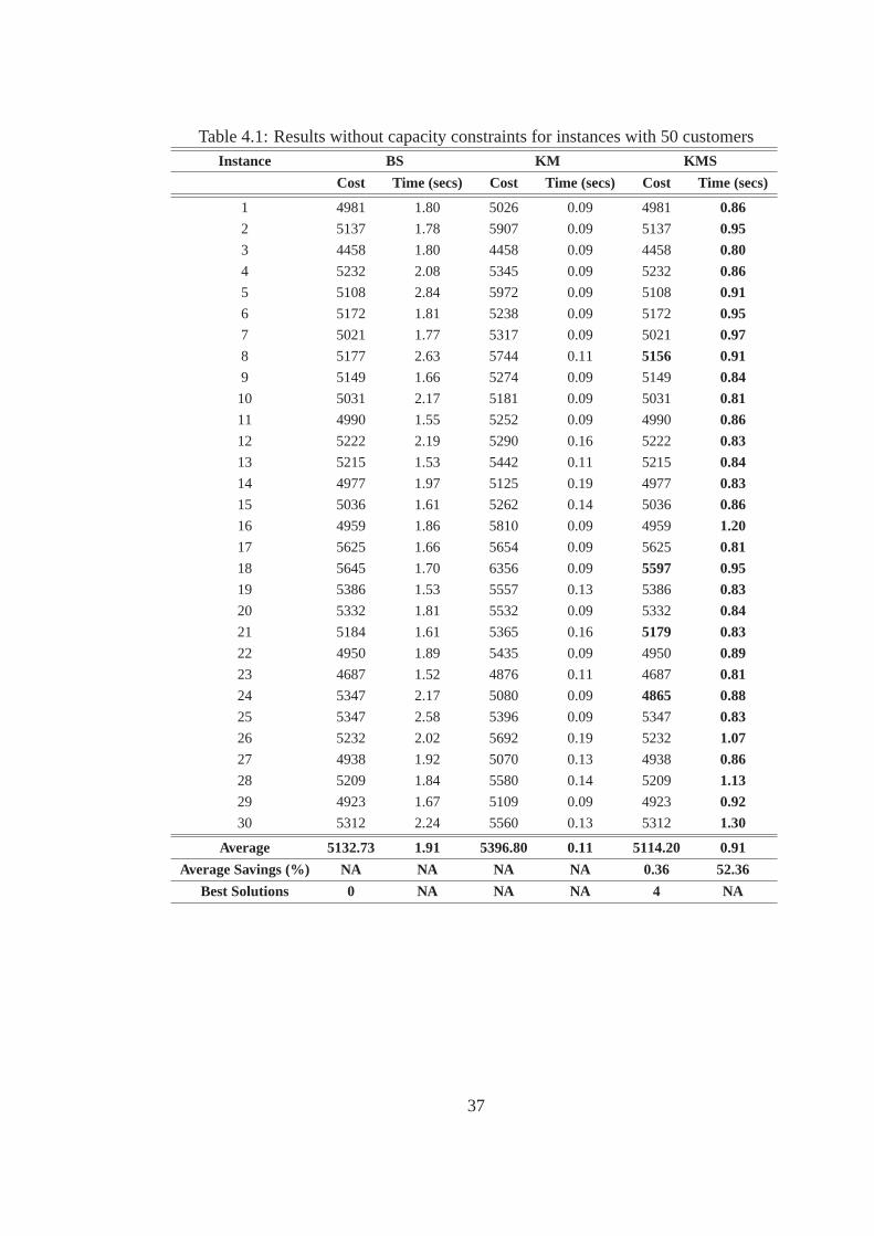
Table 4.1: Results without capacity constraints for instances with 50 customersInstance BS KM KMS
Cost Time (secs) Cost Time (secs) Cost Time (secs)
1 4981 1.80 5026 0.09 4981 0.86
2 5137 1.78 5907 0.09 5137 0.95
3 4458 1.80 4458 0.09 4458 0.80
4 5232 2.08 5345 0.09 5232 0.86
5 5108 2.84 5972 0.09 5108 0.91
6 5172 1.81 5238 0.09 5172 0.95
7 5021 1.77 5317 0.09 5021 0.97
8 5177 2.63 5744 0.11 5156 0.91
9 5149 1.66 5274 0.09 5149 0.84
10 5031 2.17 5181 0.09 5031 0.81
11 4990 1.55 5252 0.09 4990 0.86
12 5222 2.19 5290 0.16 5222 0.83
13 5215 1.53 5442 0.11 5215 0.84
14 4977 1.97 5125 0.19 4977 0.83
15 5036 1.61 5262 0.14 5036 0.86
16 4959 1.86 5810 0.09 4959 1.20
17 5625 1.66 5654 0.09 5625 0.81
18 5645 1.70 6356 0.09 5597 0.95
19 5386 1.53 5557 0.13 5386 0.83
20 5332 1.81 5532 0.09 5332 0.84
21 5184 1.61 5365 0.16 5179 0.83
22 4950 1.89 5435 0.09 4950 0.89
23 4687 1.52 4876 0.11 4687 0.81
24 5347 2.17 5080 0.09 4865 0.88
25 5347 2.58 5396 0.09 5347 0.83
26 5232 2.02 5692 0.19 5232 1.07
27 4938 1.92 5070 0.13 4938 0.86
28 5209 1.84 5580 0.14 5209 1.13
29 4923 1.67 5109 0.09 4923 0.92
30 5312 2.24 5560 0.13 5312 1.30
Average 5132.73 1.91 5396.80 0.11 5114.20 0.91
Average Savings (%) NA NA NA NA 0.36 52.36
Best Solutions 0 NA NA NA 4 NA
37
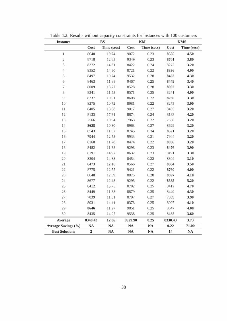
Table 4.2: Results without capacity constraints for instances with 100 customersInstance BS KM KMS
Cost Time (secs) Cost Time (secs) Cost Time (secs)
1 8640 10.74 9072 0.23 8585 4.50
2 8718 12.83 9349 0.23 8701 3.80
3 8272 14.61 8422 0.24 8272 3.20
4 8352 14.50 8721 0.22 8336 4.00
5 8497 10.74 9532 0.28 8482 4.30
6 8463 11.88 9467 0.25 8449 3.40
7 8009 13.77 8528 0.28 8002 3.30
8 8241 11.53 8571 0.25 8241 4.00
9 8237 10.91 8608 0.22 8230 3.30
10 8275 10.72 8981 0.22 8275 3.00
11 8405 18.88 9017 0.27 8405 3.20
12 8133 17.31 8874 0.24 8133 4.20
13 7566 10.94 7963 0.22 7566 3.20
14 8628 10.80 8963 0.27 8629 3.20
15 8543 11.67 8745 0.34 8521 3.20
16 7944 12.53 9933 0.31 7944 3.20
17 8168 11.78 8474 0.22 8056 3.20
18 8482 11.38 9298 0.23 8476 3.90
19 8191 14.97 8632 0.23 8191 3.30
20 8304 14.88 8454 0.22 8304 3.10
21 8473 12.16 8566 0.27 8384 3.50
22 8775 12.55 9421 0.22 8760 4.00
23 8648 12.09 8875 0.28 8597 4.10
24 8677 12.48 9295 0.22 8585 5.20
25 8412 15.75 8782 0.25 8412 4.70
26 8449 11.38 8879 0.25 8449 4.30
27 7839 11.31 8707 0.27 7839 3.90
28 8031 14.41 8378 0.25 8007 4.10
29 8646 11.27 9851 0.25 8647 4.00
30 8435 14.97 9538 0.25 8435 3.60
Average 8348.43 12.86 8929.90 0.25 8330.43 3.73
Average Savings (%) NA NA NA NA 0.22 71.00
Best Solutions 2 NA NA NA 14 NA
38

Table 4.3: Results without capacity constraints for instances with 200 customersInstance BS KM KMS
Cost Time (secs) Cost Time (secs) Cost Time (secs)
1 19910 75.28 21337 0.73 19774 32.50
2 19933 72.45 20583 0.83 19808 14.90
3 19476 67.08 20481 0.77 19463 32.00
4 19725 86.52 20207 0.69 19680 14.10
5 20091 91.86 20945 0.91 20138 50.00
6 20489 92.49 22600 0.70 20437 37.00
7 21077 73.77 21723 0.70 20827 21.14
8 19370 91.27 20002 0.78 19378 14.50
9 19387 87.39 21210 0.89 19359 36.90
10 20081 41.14 20937 0.75 19874 28.60
11 19917 70.39 20715 0.88 19878 34.30
12 19212 79.58 20657 0.70 19134 21.90
13 19490 73.58 20340 0.84 19588 29.30
14 19357 72.45 20246 0.77 19341 12.60
15 20438 82.67 21798 0.70 20392 18.40
16 20100 75.50 21561 0.69 20107 20.80
17 19933 75.17 21535 0.75 19582 22.50
18 20123 82.78 20898 0.67 20180 23.50
19 19580 78.38 20252 0.89 19580 16.70
20 19850 68.11 21170 0.78 19938 13.80
21 19586 66.05 20429 0.70 19584 19.90
22 20141 84.25 21518 0.78 19971 20.20
23 20196 76.00 21245 0.73 19779 21.60
24 20154 76.95 22447 0.83 20079 54.70
25 19813 101.00 21233 0.70 19816 25.90
26 20150 100.10 21478 0.94 20046 30.36
27 20296 88.20 21249 0.78 20255 15.60
28 19516 71.94 20295 0.69 19539 28.90
29 19790 72.13 20717 0.80 19462 16.20
30 20420 88.31 20897 0.70 20396 74.10
Average 19920.03 78.76 21024.00 0.77 19846.20 26.76
Average Savings (%) NA NA NA NA 0.37 66.02
Best Solutions 8 NA NA NA 21 NA
39
4.0.5 Results With Capacity Constraints
Tables 4.4 - 4.6 show the results of the 30 instances of data with 50, 100 and 200 customers re-
spectively for the following three heuristics: (i) basic shift (BS) algorithm, (ii) Ejection Chain (EC)
algorithm , and (iii) Ejection Chain with modified K-means (ECK) algorithm. For each instance, we
again show the value of objective function i.e., the value of the objective function, and the run time
in seconds. In addition, we show the average cost and average time across all the customers for the
three heuristics. Further, we mark in bold the best solutions found in the simulation and indicate the
total number of best solutions found. We define the best solution as the onethat is cost-wise lesser
for a particular instance among the BS, EC and ECK algorithms.
Values of parameters such asψ, ϕ, andθ are identical to the ones used in Section 5.2. Since
capacity constraints are considered, infeasible solutions can occur in thesimulations. In all the
above heuristics, we allow infeasibilities. However, infeasible solutions arepenalized according to
the degree of infeasibility by a factor ofβ. The value ofβ is initially set to 100*NC. However,β is
changed dynamically as follows: if the current solution is feasible for the given capacity constraints,
thenβ is multiplied by 0.5, otherwiseβ is multiplied by 1.5.
From Table 4.4 i.e., 50 customers case results, the EC algorithm performs better than the BS
algorithm. Also, ECK algorithm outperforms the other two heuristics. Specifically, only 2 best
solutions are found using the BS algorithm, and 3 best solutions are found using the EC algorithm,
whereas, 15 best solutions are found using the ECK algorithm. There is onan average 0.9% cost
saving that the EC algorithm generates in comparison with the BS algorithm. The ECK algorithm
produces on an average 1.68% cost savings over the BS algorithm. This clearly demonstrates that
both EC and ECK algorithms out perform the BS algorithm. The computation time required for EC
and ECK algorithms is very high when compared to the BS algorithm. The larger computational
time can be attributed to the evaluation of multiple levels of the ejection chain. Anotherinteresting
comparison is observed in the performances of the EC algorithm and the ECKalgorithm. The
ECK algorithm produces on an average 0.8% cost savings over the EC algorithm using almost the
40
same computation time. The number of best solutions found using the ECK algorithm is relatively
high. Hence, we can conclude that the use of the modified K-means algorithmas initial solution
accelerates the convergence of the solution and helps find better solutionsin lesser amount of time.
From Table 4.5 i.e., 100 customers case results, it can be observed that theECK algorithm
obtains best solutions for 22 instances. This clearly shows that the ECK algorithm produces signif-
icant performance improvement. The BS and EC algorithms obtain best solutions for only 3 and
5 instances, respectively. For the 100 customer instances, we chose stringent capacity limitations
and observed how each of the algorithms performed in extreme cases. BS and EC algorithms failed
to produce a feasible solution for several instances. In Table 4.5, instances for which the solutions
were infeasible are marked as NF. For such instances, the ECK algorithm produces best solutions.
For instances where feasible solutions were found using the BS and EC algorithms, the ECK algo-
rithm produces solutions that are in several orders of magnitude lesser interms of value of objective
function. However, these best solutions are obtained at the expense ofhigher computation time.
In Table 4.5 since many infeasible solutions are found using the BS and EC algorithms, we do not
show the average savings obtained and mark those fields as NA. For some instances 7, 10, 11, 13,
and 26, the EC algorithm performs better than the ECK algorithm. The reason isthat using the mod-
ified K-means algorithm as initial solution causes the ECK algorithm to convergeprematurely. For
instances such as 19, 23, and 28, the BS algorithm performs better than theEC and ECK algorithms.
For the above instances, the supernode construction is not effective.Hence, the BS algorithm that
examines independent customers is more effective.
Similarly from Table 4.6 i.e., 200 customers case results, it can be observed that the EC and
ECK algorithms outperform the BS algorithm. BS algorithm produces infeasiblesolutions for some
instances. Such instances are marked as NF. However, both EC and ECKalgorithms produce best
solutions for the same instances. The ECK algorithm generates the highest number of best solutions
compared to the BS and EC algorithms. Specifically, the BS and EC algorithms produce 2 and 4
best solutions, respectively, whereas, the ECK algorithm produces 24best solutions. Comparing
the performance of the EC algorithm with the ECK algorithm, we find that the ECK algorithm on
41
an average produces 1% saving over the solutions produced by the EC algorithm, and with lesser
computation time. ECK algorithm on an average produces 36% savings in terms of computation
time over the EC algorithm. Hence, we can conclude that the ECK algorithm produces better
average savings than the EC algorithm, and with lesser computation time.
To summarize from Tables 4.4 - 4.6, it can be concluded that in terms of computational cost,
the EC algorithm performs better than the BS algorithm, and the ECK algorithm performs the best.
However, the improvement in performance in terms of cost is at the expenseof higher computation
time. Also, ECK algorithm generates better solutions than those generated by the EC algorithm
with lesser computation time. Hence, we can conclude that the ECK algorithm performs best under
tight constraints because it uses the modified K-means for the initial solution and the complex
neighborhood structure construction using ejection chain coupled with supernodes. Further, we
can conclude that complex neighborhoods are essential to enhance the performance when tighter
constraints such as capacity limitations are considered. Hence, the improvement in performance in
terms of cost that the ECK and EC algorithm produce over the BS algorithm (as described also in
Section 5.3) is significantly greater than the improvement in performance that KMS produces over
the BS algorithm (as described also in Section 5.2). However, the improvement in performance in
these cases is obtained again at the expense of higher computational time.
42
Table 4.4: Results with capacity constraints for instances with 50 customersInstance BS EC ECK
Cost Time (secs) Cost Time (secs) Cost Time (secs)
1 5053 2.34 5056 8.22 5053 7.35
2 5185 2.44 5185 8.44 5185 13.49
3 5056 2.59 4694 12.45 4699 11.64
4 5722 3.08 5429 7.64 5393 9.20
5 5180 2.97 5108 11.56 5108 8.48
6 5217 3.03 5217 7.99 5182 6.88
7 5029 1.94 5029 8.34 5029 8.81
8 5379 2.13 5693 7.41 5299 11.22
9 5602 2.20 5321 9.72 5318 10.68
10 5217 2.36 5231 11.33 5217 9.33
11 5099 2.33 5142 8.53 5089 9.47
12 5365 2.45 5056 8.24 5365 10.38
13 5346 1.99 5390 12.24 5400 8.70
14 5012 2.75 5012 13.17 5012 11.45
15 5207 2.38 5160 12.69 5154 7.89
16 5003 1.95 5003 9.48 5003 10.73
17 6484 3.13 6164 11.61 5812 13.87
18 5727 2.89 5877 11.56 5785 7.69
19 5441 3.66 5441 12.83 5441 11.91
20 5332 2.02 5332 8.19 5332 8.58
21 5317 2.20 5308 9.80 5308 14.09
22 5032 2.86 5065 10.30 5024 8.15
23 4842 3.50 4842 11.99 4837 11.25
24 4899 2.38 4970 8.31 4899 9.86
25 5505 2.61 5609 7.69 5505 10.30
26 5445 3.06 5456 22.63 5404 19.92
27 5171 2.69 5171 11.33 5138 8.06
28 5428 2.44 5411 14.08 5299 8.90
29 5666 2.05 5285 12.91 5109 20.70
30 5674 2.03 5546 7.75 5554 10.66
Average 5321.17 2.55 5273.43 10.61 5231.77 10.65
Average Savings (%) NA NA 0.90 -316.08 1.68 -317.65
Best Solutions 1 NA 3 NA 15 NA
43
Table 4.5: Results with capacity constraints for instances with 100 customersInstance BS EC ECK
Cost Time (secs) Cost Time (secs) Cost Time (secs)
1 9368 13.41 8966 104.33 8955 88.40
2 10211 17.94 9295 125.58 9211 66.95
3 NF NA 9267 107.02 8963 73.61
4 NF NA 9330 68.17 9226 27.27
5 NF NA NF NA 10807 32.19
6 NF NA NF NA 10265 63.70
7 8836 16.19 8736 102.23 8891 62.25
8 8891 16.83 8560 102.41 8518 37.83
9 10059 28.99 9654 142.72 9509 73.06
10 9942 25.91 9043 99.88 9970 24.36
11 11242 176.34 9731 41.47 9882 123.98
12 8403 54.64 8306 37.30 8212 14.88
13 8770 40.58 8462 120.16 8750 27.75
14 9561 27.38 10299 73.58 9549 67.94
15 NF NA NF NA 10588 110.80
16 10599 24.86 8628 122.61 8545 193.90
17 NF NA NF NA 17120 36.34
18 NF NA NF NA 8836 66.66
19 9261 31.44 9377 99.08 9769 45.91
20 8780 15.22 8441 63.33 8426 73.06
21 NF NA NF NA 10824 35.63
22 NF NA 24920 58.05 9824 46.56
23 9351 15.59 9364 84.25 9476 274.67
24 NF NA NF NA 10365 79.73
25 NF NA 10627 68.14 9486 53.30
26 9189 14.49 8899 59.09 9238 181.20
27 NF NA 9011 80.39 8606 71.38
28 8600 21.13 8913 67.55 8743 181.70
29 NF NA NF NA 11752 42.30
30 16082 44.58 11834 134.94 10055 107.81
Average NA 19.52 7322.10 65.41 9745.37 79.50
Average Savings (%) NA NA NA NA NA NA
Best Solutions 3 NA 5 NA 22 NA
44
Table 4.6: Results with capacity constraints for instances with 200 customersInstance BS EC ECK
Cost Time (secs) Cost Time (secs) Cost Time (secs)
1 20556 114.38 20419 547.25 20386 514.77
2 20324 120.48 20030 310.19 19967 207.75
3 20345 99.97 20586 342.13 20259 363.89
4 20434 123.14 20813 256.48 20221 216.70
5 NF NA 20348 413.48 20370 339.52
6 NF NA 21115 665.41 21515 351.92
7 22531 168.33 21382 303.67 21048 183.69
8 NF NA 20196 557.69 20186 327.89
9 19689 196.06 19663 381.88 19657 403.00
10 20453 163.24 20413 320.11 20365 248.47
11 20426 219.69 20503 542.27 20305 750.28
12 19771 270.36 19912 405.20 19406 366.27
13 20405 193.09 20096 471.55 20583 376.13
14 20730 264.16 19994 377.45 19480 249.42
15 66103 129.14 20951 435.52 20939 201.86
16 21188 170.73 20557 670.45 20465 293.22
17 20167 180.63 20064 452.91 20016 255.39
18 21156 209.78 20839 392.45 20784 307.80
19 19874 186.88 20338 900.81 20013 228.30
20 20847 153.83 20189 939.99 20055 359.64
21 20511 180.00 20507 398.36 20160 164.61
22 20850 133.75 20539 561.30 20182 199.63
23 NF NA 20112 731.78 20138 193.00
24 20720 157.13 20760 384.86 20655 448.93
25 20345 124.47 20631 346.52 20357 243.02
26 NF NA 22031 410.75 20427 353.98
27 20845 198.67 20636 457.05 20586 230.84
28 19976 201.41 20052 385.72 20083 287.50
29 20453 176.84 21784 350.16 20260 187.11
30 21059 138.61 21090 366.41 20733 111.81
Average NA 142.49 20551.67 469.33 20320.03 298.88
Average Savings (%) NA NA NA NA NA NA
Best Solutions 2 NA 4 NA 24 NA
45
Chapter 5
Conclusions and Future Work
This thesis addressed the problem of meeting the multi-period demands of geographically dis-
tributed customers using a tabu search heuristic. The solution used a customer clustering strategy
that included the K-means clustering algorithm for initial solution construction,and three advanced
neighborhood search algorithms: (i) shift move, (ii) shift move with supernodes, and (iii) ejection
chain with supernodes, to accelerate convergence. In addition, two variants were developed to han-
dle the two cases where the capacity constraints of the vehicles at the warehouse may or may not
be given. We evaluated our solution and compared the utility of the three neighborhood search al-
gorithms using simulations on a well-known set of multi-period customer demand instances. Our
performance evaluation results demonstrated that using the K-means clustering algorithm greatly
aids the faster convergence of the final solution. Also, when capacity constraints are not consid-
ered, the shift move with supernodes algorithm produces notable time savings in comparison with
standard neighborhood search algorithms such as shift move. Further,when capacity constraints are
considered, the ejection chain with supernodes algorithm produces bestsolutions for cases where
solutions using shift move algorithm are infeasible. For feasible solution cases using the shift moves
algorithm, the ejection chain with supernodes algorithm produces significantcost savings at the ex-
pense of added computation time.
46
Future work could further investigate adaptive adjustment methods for computing the penalty
factor dynamically during clustering under capacity constraints. It is believe that such an investiga-
tion could produce better savings in terms of cost and time for the ejection chainwith supernodes
algorithm. Further, one may apply extensive intensification and diversification strategies such as
adaptive memory structures, and path re-linking similar to (Pacheco, 2005)for extensive exploration
of the search space. More exploration capabilities will avoid the cases of premature convergence of
solutions in our ejection chain with modified K-means algorithm.
47
Bibliography
[1] Boudia, M., Louly, M. A. O. and Prins, C., “A Reactive GRASP and Path relinking for Com-
bined Production-distribution Problem”,Elsevier Journal on Computers and Operations Re-
search, 34(11), 3042-3419 (2007).
[2] Garey, M.R. and Johnson, D.S.,Computers and Intractability: A Guide to the Theory of NP-
Completeness, Freeman Publication, New York (1979).
[3] Al-Sultan, K.S. and Khan, M.M., “Computational Experience on Four Algorithms for the Hard
Clustering Problem,Pattern Recognition Letters, 17(3), 295-308 (1996).
[4] Mourgaya, M. and Vanderbeck, F., “Column Generation Based Heuristic for Tactical Planning
in Multi-Period Vehicle Routing”,European Journal of Operational Research(2006).
[5] Brunner, J. O., Kolisch, R. and Bard, J. F., “Flexible Shift Scheduling of Medical Residents”,
Technical Report, University of Texas, Austin(2008).
[6] Osman, I. H., “Metastrategy Simulated Annealing and Tabu Search Algorithms for the Vehicle
Routing Problem”,Annals of Operations Research, 41, 421-451 (1993).
[7] Clarke, G. and Wright J.W., “Scheduling of Vehicles from a Central Depot to a Number of
Delivery Points”,Journal of Operations Research(1964).
[8] Taillard, E.D., “Parallel iterative search methods for Vehicle Routing Problem”, Journal of
Networks, 23, 661-673 (1993).
48
[9] Barbarosoglu, G. and Ozgur, D., “A Tabu Search Algorithm for theVehicle Routing Problem”,
Journal of Computer and Operations Research, 26(3), 255-270 (1999).
[10] Gendreau, M., Hertz, A. and Laporte, G., “A Tabu Search Heuristic For The Vehicle Routing
Problem”,Journal of Management Science, 40(10), 1276-1290 (1994).
[11] Kelly, J. P. and Xu, J., “A Set-Partitioning-Based Heuristic for the Vehicle Routing Problem”,
Informs Journal on Computing, 11(2), 161-172 (1999).
[12] Xu, J. and Kelly, J. P., “A New Network Flow-Based Tabu Search Heuristic for the Vehicle
Routing Problem”, Transportation Sciences, 30, 379-393 (1996).
[13] Yagiura, M. and Ibaraki, T., “An Ejection Chain Approach for the Generalized Assignment
Problem”,INFORMS Journal on Computing, 16(2), 133-151 (2004).
[14] Franca, P. M., Sosa, N. M. and Pureza, V., “An Adaptive Tabu Search Algorithm for the
Capacitated Clustering Problem”,International Transaction in Operational Research, 6, 665-
678 (1999).
[15] Ahmadi, S. and Osman, I. H., “Greedy Random Adaptive Memory Programming Search for
the Capacitated Clustering Problem”,European Journal of Operational Research, 162, 30-44
(2005).
[16] Scheuerer, S. and Wendolsky, R., “A Scatter Search Heuristic for the Capacitated Clustering
Problem”,European Journal of Operational Research, 169, 533-547 (2006).
[17] Yan, P., Liu, D., Yuan, D. and Yu, J., “Genetic Algorithm with Local Search for Advanced
Planning and Scheduling”,International Natural Computation Conference, 3, 781-785 (2007).
[18] Glover, F., “Tabu Search and Adaptive Memory Programming - Advances, Applications and
Challenges”,Advances in Metaheuristics, Optimization, and Stochastic Modeling Technologies,
Kluwer Publication ISBN 0792398440, 1-75 (1997).
49
[19] Yagiura, M., Yamaguchi, T. and Ibaraki, T., “A Variable Depth Search Algorithm with Branch-
ing Search for the Generalized Assignment Problem”,Optimization Methods and Software,
10(2), 419-441 (1998).
[20] Yagiura, M., Yamaguchi, T. and Ibaraki, T., “A Variable Depth Search Algorithm for the
Generalized Assignment Problem”,Meta-Heuristics: Advances and Trends in Local Search
Paradigms for optimization, Kluwer Academic Publishers, 459-471 (1999).
[21] Yagiura, M., Ibaraki, T. and Glover, F., “A Path Relinking Approach with Ejection Chains for
the Generalized Assignment Problem”,European Journal of Operational Research, 169, 548-
569 (2006).
[22] Diaz, J. A. and Fernandez, E., “A Tabu Search Heuristic for the Generalized Assignment
Problem”,European Journal of Operational Research, 132(1), 22-38 (2001).
[23] Cano, J. R., Cordon, O., Herrera, F. and Sanchez, L., “A Greedy Randomized Adaptive Search
Procedure applied to the Clustering Problem as an Initialization Process using K-means as a
Local Search Procedure”,Journal of Intelligent and Fuzzy Systems, 12, 235-242 (2002).
[24] Cordeau, J., Gaudioso, M., Laporte, G. and Moccia, L., “A Memetic Heuristic for the Gener-
alized Quadratic Assignment Problem”, 18(4), 433-443 (2006).
[25] Sung, C. S. and Jin, H. W., “A Tabu-search-based Heuristic forClustering”,Pattern Recogni-
tion, 33, 849-858 (2000).
[26] Glover, F., “Tabu search: Part I”,ORSA Journal of Computing, 1, 190-206 (1989).
[27] Glover, F., “Tabu search: Part II”,ORSA Journal of Computing, 2, 4-32 (1990).
[28] Queen, M., “Some Methods for Classification and Analysis of Multivariate Observations”,
Proc. of Berkeley Symposium on Mathematical Statistics and Probability(1967).
[29] Brusco, M. J., “Clustering Binary Data in the Presence of Masking Variables”,Psychological
Methods, 9, 510-523 (2004).
50
[30] Stainley, D. and Brusco, M. J., “Initializing K-means Batch Clustering:A Critical Evaluation
of Several Techniques”,Journal of Classification, 24, 99-121 (2007).
[31] Guret, C., Heipcke, S., Prins, C. and Sevaux, M., “Applications of Optimization with Xpress-
MP”, Dash Optimization Publication ISBN 0-9543503-0-8(2002).
[32] Glover, F. and Laguna, M., “Tabu Search”,Kluwer Academic Publishers ISBN 0-7923-8187-4
(1997).
[33] Pacheco, J. A., “A Scatter Search Approach for the Minimum Sum-of-squares Clustering Prob-
lem”, Journal of Computers and Operations Research, 32, 1325-1335 (2005).
51