synthetic seismograms related - harvest
TRANSCRIPT


SYNTHETIC SEISMOGRAMS RELATED TO DETAILED GEOLOGY
IN THE CELTIC FIELD, SASKATCHEWAN
A THESIS
SUBMITTED TO THE FACULTY OF GRADUATE STUDIES AND RESEARCH
IN PARTIAL FULLFILLMENT OF THE REQUIREMENTS
FOR THE DEGREE OF
MASTERS OF SCIENCE
IN THE
DEPARTMENT OF GEOLOGICAL SCIENCES
UNIVERSITY OF SASKATCHEWAN
by
Margaret Kathleen Lomas
Saskatoon, Saskatchewan
c 1983. M. K. Lomas

The author has agreed that the Library, University of Saskatchewan,
may make this thesis freely available for inspection. Moreover, the
author has agreed that permission for extensive copying of this thesis
for scholarly purposes may be granted by the professor or professors who
supervised the thesis work recorded herein or, in their absence, by the
Head of the Department or the Dean of the College in which the thesis
work was done. It is understood that due recognition will be given to
the author of this thesis and to the University of Saskatchewan in any
use of the material in this thesis. Copying or publication or any other
use of the thesis for financial gain without approval by the Universityof Saskatchewan and the author's written permission is prohibited.
Requests for permission to copy or to make any other use of
material in this thesis in whole or in part should be addressed to:
Head of the Department of Geological Sciences
University of Saskatchewan
SASKATOON, Canada

ABSTRACT
In the L10ydminster area of Saskatchewan, heavy oil commonly occurs
in thin, less than five-metre thick, vertically-stacked lenses within
the sand beds of the Lower Cretaceous Mannville Group. Seismic mapping
of the Mannville section has proved difficult due to the thinness of the
beds, the lateral variation of these beds, and the lack of acoustic
markers. The comparison of synthetic seismograms to detailed
stratigraphic and core-analysis data allowed the interpretation of
subtle seismic responses on these computer-simulated seismograms.
Synthetic seismograms, which included the effects of absorption and
dispersion, were constructed for seven closely-spaced wells located in
and near an enhanced-recovery pilot-project in the Celtic field. Input
parameters of an impulse source buried at 29.9 m and a Q curve derived
from published Q-values provided the best synthetic-seismic response to
the zones of economic importance located within the Mannville Group.
In the Celtic field, the seismic-reflection method could be used
for heavy-oil exploration or development if sufficient frequency-content
in the 60 to 115 hz range is returned from the Mannville section.
However, the dominant frequency imposed by the natural filtering of the
earth is only 39 hz in all but one of the wells studied. Data
acquisition and processing techniques must, therefore, be chosen to
accentuate the 60 to 115 hz range.

ACKNOWLEDGEMENTS
This project was supervised by Dr. Z. Hajnal, whose encouragement
and eternal optimism were greatly appreciated. I would also like to
thank Drs. B. Pandit, D.J. Gendzwill, and W.G.E. Caldwell for their
critical reviews of the manuscript in its early stages. Special thanks
go to Dr. J.A. Lorsong, who made his expertise and unpublished data
freely available to me. Dr. D.C. Ganley supplied the basic computer
code for the synthetic-seismogram program.
Research funds for.the project were provided by Petro-Canada
Exploration Inc. Data were contributed by Mobil Oil Canada Ltd. and
the Saskatchewan Department of Mineral Resources.
The author was supported by scholarships from the Saskatchewan
Research Council and the University of Saskatchewan.

TABLE OF CONTENTS
Chapter Page
1. INTRODUCTION 1
2. GEOLOGY 6
2.1 Stratigraphy 6
2.2 Ecomomic Geology 10
3. GEOPHYSICAL CONSIDERATIONS 14
4. DATA COLLECTION AND PREPARATION 18
4.1 Well Locations 18
4.2 Geophysical Logs 20
4.3 Subsurface Section 30
4.3.1 Core Units 30
4.3.2 Geophysical-Log Marker-Beds 32
4.3.3 Properties of the Surficial Layers 36
4.4 Core Analyses 39
4.5 Q Values 45
5. GEOPHYSICAL PROCESSING AND ANALYSIS 50
5.1 Synthetic Seismograms 50
5.2 Spectral Analysis 54
5.3 Model Parameters 56
5.3.1 Introduction 56
5.3.2 Geologic modelling 57
5.3.3 Q Values 70
5.3.4 Depth of Source Buri al 85
5.3.5 Input Source 94
5.4 Variation Among Wells 110
i

6. INTERPRETATION 129
6.1 Resolution Limits 129
6.2 Earth Filter 135
6.3 Physical Rock-Properti es 147
6.4 Possible Correlation to Real Seismic-Data 156
7. CONCLUSION
REFERENCES
160
161
APPENDIX A: Core-analysis data, as stored in the CA.DAT files 171
CA4B2.DAT 172
CA2D2.DAT
CA4D2.DAT
CA2BB.DAT
CA4BB.DAT
CA2DB.DAT
CA411.DAT
APPENDIX B: Listings of computer programs
CELGRF
LOGGRF
SPECAN
SYNCEL
172
173
174
175
176
177
17B
179
203
212
229
i;

Figure
1.1
2.1
4.1
4.2
4.3
4.4
4.5
4.6
4.7
4.8
4.9
4.10
5.1
5.2
5.3
5.4
5.5
5.6
5.7
5.8
5.9
5.10
5.11
LIST OF FIGURES
Location map for the Celtic pilot-project
Stratigraphic divisions of the Cretaceous Series
Data 1 ocati ons .t n the study area
Edited and unedited logs for well 288
Velocity and density values for well 2D2
Velocity and density values--Mannville portion, well 202
Core and log data--Mannville sections of
pilot-project wells
Stratigraphic marker-beds for well 2D2
Core and log data--Mannville section, well 4-11
Location map for the shallow wells
Example sheet of core-analysis results
Q values used in the study area
Well-log zones edited for geologic modelling
Parameters used for geologic modelling
Well logs and seismogram--Waseca oil-zones shaled out
Unmodified well-logs and resulting synthetic-seismogram
Well logs and seismogram--W6 oil-zone shaled out
Well logs and seismogram--W3 oil-zone Shaled out
Amplitude spectrum--unmodified well-logs
Well logs and seismogram--gas effect removed from Colony
Well logs and seismogram--MC coal-bed replaced by shale
Well logs and seismogram--W1 zone edited to appear
non-cemented
Seismogram--Q value of 20
i ; ;
Page
4
7
19
23
27
29
in
35
in
38
43
48
58
59
60
61
62
63
66
68
69
71
72

5.12
5.13
5.14
5.15
5.16
5.17
5.18
5.19
5.20
5.21
5.22
5.23
5.24
5.25
5.26
5.27
5.28
5.29
5.30
5.31
5.32
5.33
5.34
5.35
5.36
5.37
5.38
5.39
,
Seismogram--Q value of 50
Seismogram--Q value of 100
Amplitude spectrum--Q value of 20
Amplitude spectrum--Q value of 50
Amplitude spectrum--Q value of 100
Seismogram--standard Q function
Amplitude spectrum--standard Q function
Seismogram--Q value of 20; plotted without gain
Seismogram--Q value of 50; plotted without gain
Seismogram--Q value of 100; plotted without gain
Seismogram--impulse source at 0.0 m
Seismogram--impulse source at 9.8 m
Seismogram--impulse source at 29.9 m
Seismogram--impulse source at 46.7 m
Amplitude spectrum--impulse source at 0.0 m
Amplitude spectrum--impulse source at 9.8 m
Amplitude spectrum--impulse source at 29.9 m
Amplitude spectrum--impulse source at 46.7 m
Velocity-type Ricker-wavelet
Phase and amplitude spectra of Ricker wavelet
Seismogram--60 hz Ricker-wavelet source
Seismogram--80 hz Ricker-wavelet source
Seismogram--100 hz Ricker-wavelet source
Seismogram--140 hz Ricker-wavelet source
Seismogram--180 hz Ricker-wavelet source
Seismogram--220 hz Ricker-wavelet source
Amplitude spectrum--60 hz Ricker-wavelet source
Amplitude spectrum--80 hz Ricker-wavelet source
iv
73
74
76
77
78
79
80
82
83
84
86
87
88
89
90
91
92
93
95
96
98
99
100
101
102
103
104
105

5.40
5.41
5.42
5.43
5.44
5.45
5.46
5.47
5.4S
5.49
5.50
5.51
5.52
5.53
5.54
5.55
5.56
5.57
5.5S
6.1
6.2
6.3
6.4
6.5
6.6
6.7
6.S
6.9
Amplitude spectrum--100 hz Ricker-wavelet source
Amplitude spectrum--140 hz Ricker-wavelet source
Amplitude spectrum--1S0 hz Ricker-wavelet source
Amplitude spectrum--220 hz Ricker-wavelet source
Well logs and synthetic seismogram for well 4B2
Well logs and synthetic seismogram for well 202
Well logs and synthetic seismogram for well 402
Well logs and synthetic seismogram for well 2BS
Well logs and synthetic seismogram for well 4BS
Well logs and synthetic seismogram for well 20S
Well logs and synthetic seismogram for well 4-11
Amplitude spectrum--wel1 4B2
Amplitude spectrum--wel1 202
Amplitude spectrum--we11 402
Amplitude spectrum--we11 2BS
Amplitude spectrum--we11 4B8
Amplitude spectrum--we11 208
Amplitude spectrum--we11 4-11
Synthetic-seismogram cross-section
Time gates through seismogram--impu1se source
Amplitude spectrum--impu1se source
Amplitude spectrum--time gate from 0.15 to 0.25 s
Amplitude spectrum--time gate from 0.25 to 0.35 s
Amplitude spectrum--time gate from 0.30 to 0.40 s
Porosity values, well logs, and core data
Key to the core-data symbols
Permeabi1ity-to-air values, well logs, and core data
Clay-content values, well logs, and core data
v
106
107
lOS
109
112
113
114
115
116
117
118
119
120
121
122
123
124
125
126
136
140
142
143
144
149
150
152
154

6.10 Oil saturation, presence of gas, well logs, and core data 157
vi

Table
1.1
4.1
4.2
4.3
4.4
4.5
5.1
6.1
LIST OF TABLES
A.P.I. densities of liquids
Summary of acoustic-well-log editing
Summary of density-well-log editing
Surficial-geology data
Stratigraphic marker-bed depths
Summary of in situ measurements of Q
Summary of reflection data from the modelled zones
Theoretical resolution of the modelled zones
Page
3
24
25
40
41
47
65
132
vii

CHAPTER ONE
INTRODUCTION
"The relationship of borehole data and seismic data should be such
that rock properties can be assigned to the seismic trace" (Stone,
1980). An understanding of the detailed relationship between a seismic
trace and the geologic section that it represents is essential to the
stratigraphic interpretation of seismic sections. Too often, the
relationship is not fully appreciated and subtle expressions in the
seismic trace are not interpreted correctly, or are not even recognized.
The heavy-oil deposits of western Canada are located in a complex
geologic environment; the thin beds and lateral variability of these
beds make seismic records difficult to interpret. Although the seismic
method would be a great aid to exploration and development, it is seldom
used �Jith success. A theoretical study of the detailed relationship
between a geologic section in the heavy-oil area and its calculated
seismic response was undertaken to test the applicability of new,
high-resolution, seismic-reflection methods to this difficult
environment. The term 'high resolution' is used here to mean the
recording of seismic frequencies above the normal exploration range
(Sheriff, 1973).
Lower Cretaceous rocks in the Canadian portion of the Western
Interior basin contain viscous oil along a broad arcuate belt that
extends from the Peace River oil sands of northwestern Alberta into the
North Battleford-L10ydminster heavy oil district of west-central
Saskatchewan. The deeper reservoirs at the southeast end of the belt
contain oil that is more paraffinic, of lower specific gravity (higher
A.P.I. gravity), and of lower viscosity than that oil in the shallower

Page 2
northwestern reservoirs (Vigrass, 1965). A.P.I. gravity is a standard
adopted by the American Petroleum Institute for denoting the specific
weight of oil s (Gary et.!!_., 1974, p 32). Wennekers et al • (1979 )
distinguished heavy oil as having an A.P.I. gravity of between 10 and
25 degrees and tar-sands oil as having as A.P.I. gravity of less than
10 degrees. These and other A.P.I. values are shown in Table 1.1.
The Lloydminster area is the site of maximum heavy oil accumulation
within the viscous-oil belt of western Canada. Its reserves are
estimated to be 4.5 billion cubic metres, of which 0.45 billion cubic
metres are economically recoverable using tertiary production methods
(Wennekers et �., 1979). The Lloydminster heavy oil area is located
along the Alberta-Saskatchewan border, approximately 450 to 540 km north
of the United States border. The location of this study is the tertiary
recovery pilot project in the Celtic heavy-oil field. The pilot project
occupies the southeast quarter of Section 10, Township 52, Range 23 west
of the Third Meridian (see Figure 1.1) and will hereafter be referred to
as the Celtic pilot project. In 1980, the Celtic pilot project was
unique within the Lloydminster area because of its large quantity of
high quality cores, geophysical logs, and eXisting geological studies.
In addition, the geology of the Celtic field is fairly typical of that
of the Lloydminster area (Haidl, personal communication, 1981; Lorsong,
1981)
The goal s of thi s study v/ere to
1) Investigate the potential usefulness of the seismic reflection
technique in the heavy-oil area.
2) Develop a method to evaluate the high-resolution seismic technique in
the study area.
3) Study the detai 1 ed rel ati onshi p between the subsurface geology of the

Page 3
TABLE 1.1. A.P.I. DENSITIES OF LIQUIDS
LIQUID A.P.I. DENSITY REFERENCE
tar sand oil less than 10 degrees Wennekers et al. (1979)--
fresh salt-water 10 degrees Wennekers et al. (1979)--
heavy oil 10 to 25 degrees Wennekers et ale (1979)--
conventi onal oil 25 to 40 degrees Mossop (1978)

Page 4
18
7
13
R.23
Tp.52
Tp.50
10
10
6
Tp.52
PILOT4
P ROJ ECT--+-- '/r-�-+-----+--
31
Tp.51
30
19
R.23 W3M.
oMILES
2
oKM.
2
R.22
.Figure 1.1 - Location map for the Celtic pilot project.

Page 5
study area and the theoretical seismic trace computed from it.
4) Determine the parameters for synthetic seismogram construction that
will best detect the economically important intervals.
5) Evaluate the potential of the seismic method as a tool for
exploration and reservoir evaluation in the study area and, if possible,
extend the results to other areas.

Page 6
CHAPTER TWO
GEOLOGY
2.1 Stratigraphy
Attention has been focussed on the Lower Cretaceous sequences of
western Canada because of the presence of deposits of conventional oil,
heavy oil, tar sands, natural gas, and coal. As a result of extensive
drilling, these rocks have been widely studied in the subsurface. In
general, Cretaceous strata were deposited in north-south trending facies
belts, as successive seas transgressed and regressed. The Cretaceous
sequence is, therefore, highly variable across the Western Canada basin,
making correlation difficult in an east-west direction (North and
Caldwell, 1975). For this reason the stratigraphic section discussed
will be restricted to that of the heavy oil area near Lloydminster,
where three major Cretaceous units are present: the Mannville Group,
the Colorado Group, and the Montana Group. A stratigraphic column for
the Cretaceous rocks of the study area is given in Figure 2.1.
The Mannville Group in the Lloydminster area is a sandstone-shale
sequence of Late Neocomian to Middle Albian age (Christopher, 1974, p.
49-50; 1980) that lies with a slight angular unconformity on eroded,
mainly carbonate strata of Devonian age. Relief on the pre-Cretaceous
surface is subdued, with shallow basins and valleys and southwesterly
dip. White and von Osinski (1977) described the Mannville as comprising
an interbedded sequence of sandstone, shale, and mudstone. These
sandstones are actually weakly consolidated to uncemented sands that are
fine grained to silty, and quartz rich. Minor feldspar, siderite,
glauconite, garnet, tourmaline, zircon, chlorite, pyrite, and limonite
may be present. The total thickness of the Mannville Group varies from
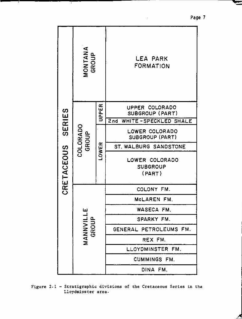
Page 7
<t
Zo-<t:) LEA PARK.... 0
FORMATIONZo::o(,!)�
a:UPPER COLORADO
enl&J
� SUBGROUP (PART)W c,- � 2nd WHITE - SPECKLED SHALEa::
W0
Co- LOWER COLORADOen
<t:) SUBGROUP (PART)0::000: a:
ST. WALBURG SANDSTONEen -1(,!) l&J
:::l0 3:
0u 0
..JLOWER COLORADO
W
o SUBGROUP
« ( PART)f-
W
a::: COLONY FM.(J
McLAREN FM.
LLI WASECA FM.-1
-10- SPARKY FM.-:)
>0GENERAL PETROLEUMS FM.Za::
Z(,!)<t REX FM.�
LLOYDMINSTER FM.
CUMMINGS FM.
DINA FM.
Figure 2.1 -
Stratigraphic divisions of the Cretaceous Series in the
Lloydminster area·

---�........
Page 8
80 to 230 m, \�th regional thinning to the southwest (White and von
Osi nski, 1977).
Nine stratigraphic units have been informally recognized within the
Mannville Group on the basis of electric log characteristics. However,
the lateral variation, repetition of similar lithotypes in a vertical
sequence, and the absence of marker beds preclude the identification of
any unit by a characteristic electric-log response (Haidl, 1980; Gross,
1980). Correlations over long distances are highly speculative (White
and von Osinski, 1977). In spite of this limitation, the above authors
agree that the stratigraphic scheme is useful in that it provides a
framework in which to discuss Mannville geology and to place a segment
of rock in relative stratigraphic position. The stratigraphic names
used are, from oldest to youngest: Dina, Cummings, Lloydminster, Rex,
General Petroleums (G.P.), Sparky, Waseca, McLaren, and Colony
formations. The names were adapted by Fuglem (1970) from a well
established drillers' terminology that originated near the town of
Lloydminster. His descriptions were later modified by Vigrass (1977)
and the divisions were raised from member to formational status by Orr
et al. (1977).
For part of Early Cretaceous time, the Lloydminster area was
situated near the edge of an epicontinental sea (Robson, 1980). This
accounts in part for the wide variety of depositional environments and
the lateral variability of the facies units throughout the Mannville
Group. It is generally agreed that the Dina formation is a fluvial and
alluvial-plain deposit, filling topographic depressions (Williams, 1963;
Orr et �., 1977; Vi grass, 1977; Gross 1980). The Cummi ngs,
Lloydminster, Rex, G.P., and Sparky formations are mainly marine to
nearshore marine (Fuglem, 1970; Orr et �., 1977; Vigrass, 1977;

Page 9
Gross, 1980). In contrast, the Waseca, t4cLaren, and Colony formati ons
are a subject of controversy with regard to depositional environment;
i nterpretati ons range from fl uvi al (Putnam, 1980) through coastal mari ne
( Lorsong, 1979).
The total thickness of Mannville sediments in the Celtic field is
approximately 200 m. All nine formations are present, with the Dina
resting directly on Devonian carbonates of the Duperow Formation. The
strata are draped over a prominent, southeast-trending structural arch,
the pilot project area being located on the northeast edge of this arch
(White and von Osinski, 1977). A complete description of the lithotypes
present in the cored sections of the Celtic pilot project is presented
in section 4.3.1.
The Mannville Group is overlain abruptly, and probably
disconformably, by the marine silts and shales of the Colorado Group.
In Saskatchewan, the division into upper and lower subgroups of the
Colorado is made at the base of the Second White-Speckled Shale. The
division between the Upper and Lower Cretaceous Series is taken
approximately 20 to 30 m below the top of the Lower Colorado Subgroup,
at the bottom of the Fish Scale Marker (Simpson, 1975). The Fish Scale
Marker was not identified on the logs used in this study. Simpson
(1975) places minor unconformities at the base of the Fish Scale Zone
and at the base of the Lower Colorado.
The Lower Colorado Subgroup is of Middle Albian to Late Cenomanian
age (North and Caldwell, 1975). It is approximately 140 m thick in the
study area. The sequence is characterised by mudstones with subordinate
silt and sand layers. The St. Walburg Sandstone is the only readily
identifiable marker within the Lower Colorado on the geophysical logs
recorded in the study area. There the sandstone is approximately 20 m

Page 10
thick. Simpson (1975) described the St. Walburg Sandstone as being
composed of horizontally laminated and micro-cross-1aminated, very fine
grained sandstones that were deposited as tidal ridges.
The Upper Colorado Subgroup is of Turonian to Late Santonian age
(North and Caldwell, 1975). It is only 40 m thick in the area of study,
due to its northeasterly thinning. The Upper Colorado in west-central
Saskatchewan is composed of two principal calcareous units. The
thickest of these is the First White-Speckled Shale, which rests with
minor angular unconformity upon the Second White-Speckled Shale (North
and Caldwell, 1975). In the area studied the Second White-Speckled
Shale is only about 6 m thick but is a reliable marker on the
geophysical logs.
Near L10ydminster, the Upper Colorado sha1ey chalks are directly
over1 ai n by the Lea Park Formati on of the �10ntana Group. North and
Caldwell (1975) attributed an Early Campanian age to the Lea Park and
argued for a minor unconformity at its base. In the Celtic pilot
project, the Lea Park is located in the uppermost 230 m of the bedrock
section and, based on the geophysical logs, forms an apparently
homogeneous sequence of argillaceous rocks.
2.2 Economic Geology
In the Lloydminster area, heavy oil is produced from quartzose
Mannville sands with porosities exceeding 30 per cent and with
permeabi1ities greater than one darcy (Fug1em, 1970). Lorsong (1981)
studied controls on oil emplacement in a small area believed to be
typical of the L10ydminster region. He concluded that oil is trapped
1 aterall y and vertically by faci es changes and by cemented zones �,i thi n
the 1 ess quar·tz-ri ch sands. In the cemented zones, porasi ty is reduced

Page 11
to virtually nil. On a larger scale, however, the overall distribution
of oil is definitely structurally controlled. Strata of the Mannville
Group dip gently to the southwest, at approximately 5 m/km (Vigrass,
1977). In general the sites of maximum oil accumulation change updip,
from the basal sands (Dina formation) in the southwest, through the
Sparky sands (near the Alberta-Saskatchewan border), and to the Colony
sands in the northeast. Nevertheless, heavy-oil fields may produce from
up to eight major lenses of oil in different sand layers (Wennekers et
�., 1979). The Celtic field hosts oil accumulations in the Rex, G.P.,
Sparky, Waseca, and McLaren formations. The Waseca and Sparky
formations of this field were estimated to contain approximately
16,500,000 cubic metres of oi1-in-p1ace, of which about 1,000,000 cubic
metres was recoverable (Saskatchewan Department of Mineral Resources,
1979, p. c-2).
A broad doma1 structure supports the L10ydminster region
(Christopher et�., 1971) and, as was mentioned in the previous
section, the Celtic field is located over a northeasterly trending
ridge. White and von Osinski (1977) reviewed the structure of the
Mannville Group and concluded that the regional dip is interrupted by
local structures resulting mainly from draping and compaction over the
pre-Cretaceous unconformity. This is complicated by downwarps related
to dissolution of Devonian Prairie Evaporite salt. They also noted that
most heavy oil pools are associated with gentle highs and that none
occurred in structurally very low sands. Moreover, in pool areas the
strata are nearly horizontal.
According to Wennekers et il. (1979) there are thirty major pools
in the Lloydminster heavy-oil region. Production from anyone well is
marginal. Within established pools, where A.P.I gravities usually range

Page 12
from 13 to 18 degrees, primary production averaged only 5 per cent
(White and von Osinski, 1977; Vigrass 1977). These same authors agreed
that with presently available methods for secondary recovery, such as
waterflooding, the production rises to about 8 per cent. Based on these
data, the reserve figures of Wennekers et�. (1979) imply that
tertiary-recovery methods, such as steam and fire flooding, could
increase production to about 25 per cent. Although recoveries are poor
and the oil lenses are thin, the shallow location, the large areal
extent, and the vertical stacking of the lenses make the area
economically attractive.
Traditionally, most exploration for heavy oil was accomplished
drilling. Because the oil-bearing horizons are multiple, shallow, and
usually cover a large area, drilling was one of the cheapest and surest
ways to assess the resource. It is now recognized that the information
produced by drilling alone is not of adequate quality. White and von
Osinski (1977), Wennekers et�. (1979), Gross (1980), Haid1 (1980),
and Lorsong (1980) all agreed that correlations based solely on
geophysical logs are unreliable; log signatures do not relate to unique
geological sequences. Even when cores are taken, accurate correlation
over any distance is made impossible by the absence of marker beds
within the Mannville Group and by the extremely variable nature of the
geology. Lorsong (1980) and Wennekers et�. (1979) provided examples
of two cases where infill drilling between drill holes that were already
correlated changed the geological interpretation radically. Based on
his work with cored sections in the Celtic pilot project, Lorsong (1980)
concluded that"
•.• we1ls located 140 m apart represent the maximum
spacing for confident prediction of sand body geometry." When spacings
of 140 m are required, drilling is no longer a quick or cheap method of

Page 13
exploration and development. A method is required that will provide
more continuous coverage of the subsurface. Drill holes could then be
selectively placed where they would provide the most useful information.
The seismic reflection-method provides much more detailed lateral
resolution of the data-collection sites than does drilling. However,
while gaining in lateral resolution, the seismic method loses in
high-resolution, seismic-acquisition and processing methods, coupled
vertical resolution. In the last few years some limited success has
been obtained by using high-resolution techniques, particularly if the
oil bearing horizon is thick. Focht and Baker (1979) and Dunning et !l.
(1980) described exploration successes using reflection seismology. In
both cases, the reservoirs mapped were channel deposits, which are much
thicker than the blanket sand reservoirs containing the majority of the
heavy oil reserves. Special care and the most up-to-date knowledge of
with a detailed understanding of the geology and its seismic expression,
will be necessary before seismic mapping will succeed in all heavy oil
environments.

Page 14
CHAPTER 3
Geophysical Considerations
pn+l Vn+1 -
pnVn
Seismic modelling is a method of computer simulation of the seismic
response from a set of input values. Synthetic seismograms are
one-dimensional seismic models that simulate a single seismic trace from
well log data. The primary use of synthetic seismograms is as a tool to
correlate between known borehole geology and a seismic response obtained
near the borehole.
The preferred input data for synthetic seismogram construction are
the velocity log (the measurement of interval transit-time with depth)
and the density log. The product of the velocity and density, or the
acoustic impedance, of the subsurface layers controls the seismic
reflections. The amplitude of the reflection from a boundary separating
two media is directly proportional to their contrast in acoustic
impedance, and is measured by the reflection coefficient R. For normal
incidence on an interface that separates layers of densities pnand pn+1
and velocities Vn and Vn+1,
R =
pn+1 Vn+1 + pnVn
To construct a simple synthetic-seismogram, velocity values from logs
are digitized and integrated to form arrays in travel time. Then,
density and velocity values are combined in the above formula and
converted into an array of reflection coefficients versus travel time.
Finally, the reflectivity series is filtered to simulate a propagating
wavelet.
Synthetic seismograms have been used since the late 1950s and in

"',--�"--------�"""--""""------------------------------��
Page 15
the early methods of construction many assumptions were made.
Assumptions such as a perfectly-elastic earth, constant density, the
nonexistence of multiples, plane waves, normal incidence, and noiseless
conditions allow easier computation of the synthetic seismogram but are,
in general, not valid and therefore make correlation of the synthetic
seismogram to the true seismic response difficult. Obviously, a balance
must be struck between the ease of synthetic-seismogram construction
(and, therefore, the cost), and the degree of sophistication of the
model that the target requires. It is important to note that even if
the data sets were perfect, and no invalid assumptions were made, the
inherent differences in the seismic and log data preclude exact
correlations (Sheriff, 1977).
Synthetic seismograms should be as realistic as possible,
especially in an area of complicated geology such as Lloydminster. The
geology there presents special problems to the seismic method and these
must be included in the seismic models or comparisons between the two
will not be possible.
The oil-bearing beds in the study area are thin, typically only 4
or 5 m thick. The vertical resolution or detection of these beds
necessitates high frequency-content in the propagating wavelet. Widess
(1973) defined the ideal limit of resolution as occurring at a bed
thickness of one eighth of the predominant Havelength. Beds thicker
than this limit may be resolved--that is, the reflections from the upper
and lower interfaces of the bed will be separate in time. On the other
hand, beds thinner than this limit will not be resolved, but they may be
detected, even when their thicknesses are considerably less than one
eighth of the predominant wavelength. The limit of detection also
depends on the signal to noise ratio.

Page 16
The lateral variability of Mannville sediments in the area of
interest necessitates considerations of lateral resolution. Seismic
waves do not reflect from a point, but from an area on the reflecting
surface called the Fresnel zone. The size of the Fresnel zone depends
on the predominant frequency content of the seismic signal; high
frequencies will produce a smaller Fresnel zone than low frequencies.
The unconsolidated nature and shallow occurrence of the Cretaceous
sediments in the area of study suggests that absorption of seismic
energy will be a problem. Absorption is a specific type of attenuation
in which some of the energy of a seismic wave is converted into heat
while passing through a medium (Sheriff, 1973). Reported absorption
measurements of rocks (Ganley, 1979) show trends of decreased absorption
with increasing consolidation and depth of burial. For this reason,
weathered surficial-rocks should be particularly absorptive. Absorption
preferentially reduces the amplitude of the higher frequency components
of the seismic signal; in consequence, the high frequencies required
for vertical and lateral resolution-of the subsurface may be attenuated
before they reach the beds of interest.
The interbedded nature of the Mannville sequence presents another
formidable problem--that of attenuation of the seismic wavelet caused by
intrabed, or short-path, multiples. In cyclically-bedded sequences in
which the reflecting interfaces alternate in sign, O'Doherty and Anstey
(1971) recognized that short-path multiple reflections can have the
effect of delaying the pulse, broadening the pulse, and magnifying the
low frequency portion of the pulse transmitted through the layered
sequence. The effect of these multiples is similar to the high-cut
effect of absorption and their results may be confused (Anstey, 1977, p.
139). Schoenberger and Levin (1978) measured the contribution of the
Page 17
attenuation caused by intrabed multiples and concluded that this effect
contributed an appreciable portion (15 to 70 per cent) of the total
observed attenuation. As in the case of absorption, the important high
frequency content of the propagating wavelet is reduced.
To simulate the effects discussed above, the method of synthetic
seismogram construction must be relatively complex. The computer
program was written by D. Ganley and is described in Ganley (1981).
All orders of surface and internal multiple reflections are calculated
by this program, and therefore, any attenuation of the waveform due to
intrabed multiples will be included. The program allows for the input
of both velocity and density data in the calculation of the reflectivity
series. Effects of absorption and dispersion are included in the
synthetic seismogram by specifying Q, a measure or absorption, for each
input interval. As well, the effect of the highly absorptive surficial
layers may be investigated by simulating the burial of the seismic
source at any desired depth. The above features make the construction
of the synthetic seismogram more realistic and, as a result, more easily
correlated to real seismic reflection data. The assumption of plane
waves and the normal incidence of these waves on flat-lying interfaces
is made, but this is a reasonable approximation for comparison with
near-source geophones when dips are small. The specifics of this method
of synthetic-seismogram construction will be discussed in section 5.1.

Page 18
CHAPTER FOUR
DATA COLLECTION AND PREPARATION
4.1 Well Locations
Six wells within the area of the Celtic pilot project and one well
just outside the pilot area were chosen for this study. The six \/e11s
from within the pilot project lie 140 m apart along cross-section AA' in
Figure 4.1. The seventh well is located at L.S.D. 4, Sec. 11, Tp.
52, R. 23, W3M. At the closest point it is approximately 725 m from
the section AA'. The wells within the pilot project are referred to by
the first part of their L.S.D. location (for example, 2D2) and the well
location outside the pilot project is abbreviated to 4-11.
The six we l l s along section AA' vere chosen for the present study
because of their superior log and core data. In addition, these wells
form a diagonal cross-section across the pilot project and perpendicular
to the local strike of the Mannville strata. All of these six wells
produce oil, with pay zones in the G.P., Sparky, McLaren, and Waseca
formations. A dry well would have facilitated comparison between the
seismic character of producing and non-producing we l l s , Unfortunately,
there were no dry wells wi th acousti clogs \/i thi n the boundari es of the
Celtic field. The Mannville geology of the seventh well, 4-11, is
rather different from the other six wells; the Waseca formation is
severely reduced in thickness and the sands of the Sparky formation have
been replaced by a thick sequence of shale. Although the status of well
4-11 is that of an oil producer, it now produces only from the McLaren
formation (Saskatchewan Department of Mineral Resources, personal
communication, 1983) and provides an example of a well in which the
important Waseca oil zones are poorly developed.

Page 19
@�r� 1h@��jjU@IM� UIM irlH)jg �jglhnc
I?Ul6@ii' 1?@.©J)��1f
R.23 W3M.
I
I
rII 10 I 9 12
I
10fI
zeT 207 101 I 2CI 20aAI
®I.. ®1ZJII'" I•
}!J6I.• 4817
4A1 4888 5
®T7111 • I •
,...
ZIT 2Al I �...
2A.
, ®...•
�r------ -
....
�C2-T021----,-
1--._----4CI
•la.
•4'.
•
2CZ 202 I 2el 201
®Ia. •a5111 ®I3. ®4a.
3
484(.2 I 481I •
4A2• ®Ia• 4-11-52-2313
A21111
I 2BI -31.2BZ 2Al 2AI
• ®17.I
®ZIIII•
I II
I
Ic I 0
I
I
II
----14---,..--- 15 I. 13I I
I 3I
•
II
I
8I I
r-4--I
I z I I
I t
Tp.52
N
LSD BREAK OOWN o 200 400
zcz• PRODUCING WELL LOCATION
� WATER DISPOSAL WELL LOCATION
® WELL LOCATION WITH DIGITIZED ACOUSTIC AND DENSITY LOG
• WELL LOCATION WITH DIGITIZED ACOUSTIC LOG ONLY
@Ia.. METRES OF CORE RECOVERED FROM WELL
A-AI WELLS USED IN SYNTHETIC SEISMOGRAM STUDY
SeAlE I. METRES
NOTE - WELLS ARE REFERENCED BY THE FIRST THREE CHARACTERS OF THE
LANO SURVEY DESIGNATION (eg.,2B8)' THE OFFICIAL NAME OF EACH
OF THESE WELLS IS MOBIL CELTIC XXX -10- 52-23 W3M, WHERE XXX
IS THE THREE- CHARACTER DESIGNATION.
Figure 4.1 - Data locations in the study area·

Page 20
4.2 Geophysical Logs
A large suite of logs, comprising induction-electric logs, a
compensated-density log, a compensated-neutron-porosity log, natural
gamma-ray logs, caliper logs, a borehole-compensated acoustic-log, and
sometimes a spontaneous-potential log is available for each of the six
wells from the pilot project. Well 4-11 lacks only the density and
neutron logs. Hole conditions for the wells in the pilot project should
be similar, �ince all were drilled within a short period of time (late
1978 and early 1979) and by the same crew, who were using the same
equipment (Lorsong, personal communication, 1981). This means that
differences between the log suites of the wells are more likely due to
geologic changes than to differing hole conditions. All of the wells,
with the exception of 288, were logged by Schlumberger of Canada. Well
288 was logged by Dresser Atlas.
Well-log data must be in digital form in order to construct a
synthetic seismogram. The original digital field-recordings of the logs
were used for wells 482, 202, 408, and 208. The logs for wells 288,
488, and 4-11 were digitized by Rileys Datashare International Inc.
from analogue copies of the logs. A 0.2 m digital interval was used for
all six of the pilot-project we l l s , Well 4-11 was drilled in 1969, and
as its logs are non-metric, the digital interval used was one-half foot
(.1524 m). A 0.2 m sample interval will allow beds of greater than 0.4
m thickness to be represented.
The next step in preparing the logs was editing. The stratigraphic
interpretation of seismic records is based on the ability to correlate
seismic character to the subsurface geology. As it is well-log data
that provide the � situ physical-properties of the subsurface section,
it is extremely important that they provide the most accurate

Page 21
information possible. Crain and Boyd (1979) felt that most
geophysicists underestimate the severity of the editing problem.
Either mechanical log-problems or environmental conditions may
cause portions of well logs to contain data that are significantly
different from the true, 22 situ formational properties (Ausburn, 1977).
Mechanical problems could include: effects caused by imperfectly
calibrated logs, cycle skip caused by gain settings that are too low,
and noise spikes caused by instrument or electronic noise.
Environmental conditions are generally related to poor hole-conditions,
such as erosion of the borehole wall, but could also include gas
effects, which can reduce the measured velocity appreciably even when
gas is present in concentrations as low as 5 per cent by volume
(Domenico, 1974). In addition, almost all formations, particularly the
softer, less competent ones, are altered when a borehole is drilled
through them (Ausburn, 1977). Shales cave, erode, absorb water, and
swell in response to drilling and exposure to mud filtrate. On the
other hand, sandstones are less affected but are altered by relaxation,
erosion, and invasion of mud filtrate.
There are 'bJO maj or facets of log edi ti ng (Ausburn, 1977). The
first is to recognize that bad data have been recorded, and the second
is to try to determine better values, which can be substituted for the
bad ones. The bad data recognized in logs used in this study were
mainly as a result of hole conditions, and cycle skip and noise due to
gas effects. Density logs are often affected by rough or washed-out
hole conditions. Acoustic logs are affected less often than density
logs. Bad data were replaced based on empirical observations of trends
in other holes where the data were better. In some severely altered
zones, published velocity and density values for similar rocks were used

Page 22
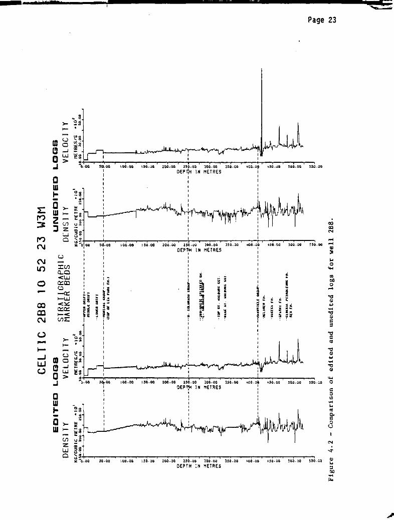
as a guide. Figure 4.2 shows a comparison of the unedited and edited
density and velocity curves for well 288. The logs are plotted at the
same horizontal scales so that the severity of the editing problems may
be appreciated.
A series of checks was made on the density- and acoustic-log data
in each well. The calibration was examined to ensure that it had not
changed during the logging run. The starting depths of the logs were
altered to be sure that both logs started at the same subsurface horizon
and that no spurious events were included due to the effect of the
surface casing. The depths of certain distinct events were compared to
be sure that they were the same on both the density and acoustic logs;
this was possible because both the density and velocity logs were run
with a simultaneous natural gamma log. Lastly, computer plots of the
digitized density and velocity values were made and compared. Several
wells were found to have discrepancies of up to 0.6 m between the depths
of the same events in the acoustic and velocity logs. Most of these
cases occurred only over a portion of the log, but well 288 was found to
have a di fference of between 0.2 and 0.4 m over the enti re 1 ength of the
logs. A computer program was written to shift the data. However, when
the synthetic seismograms computed using shifted and non-shifted data
were compared there was no visible difference, that is, the rock
velocities were low enough that there was no visible difference at the 1
ms sampling interval used for the synthetic seismograms. These small
differences in log depths were, therefore, ignored.
The caliper logs were checked for hole rugosity and washouts. Four
areas of poor borehole conditions vere encountered in the wells. These
are listed in the summaries of well-log editing presented in Tables 4.1
and 4.2. Bad data due to hole conditions were corrected by replacing
..,
<>
D
<>
<>
o
,..,
-0 ...
......
:r!'<>
_0
:z
3'"
,..,0-f0:Uo,..,0'"
CELTIC 288 10 52 23 W3M
I
MEIRES/S .'02
0.11.11(1 10.0(1 50.110
8
EDITED LOGS
DENSITY VELOCITYSTRATIGRAPHICMARKER BEDS
UNEDITED LDGS
DENSITY VELOCITY
KG/CUOIC METRE ·10'
o'�Q·I)O lUI).QQ lliO.QQ
<>
D
METRES/S ., 02
0\1)·011 31).(1(1 liO.QQ
s
KG/CUOIC MEIRE .'0'
.,1!oO.OO 'lIa.oo 2S0.00
-""rfa IIftlfJ-- -- -- -- - - - --.
··nIDllLE IIlIlfl g
...
o
<>
o
..
..
<>
"
<>
"lllllUl IIftlrr
-- -- - -- ----Pe»
<>
..
- - - --- -
---._U., ,,11_----- -- --- Q.
nor Of lEA "." fn., g
<>
<>
<>
<>
<>
D
..
o
<>
o
oo
..
o
<>
o
...
D
D
<>
...
'"
<>
<>
{..,
f..
t..
<> <> <><> c. C>
g s 8o _ 0 0
,.., ,..,,,,,
-- - - - - - -- - -i � - - - - -- - - - - -- - --.y. &OLIIII'PII lillQOf'---- - - - -i � - - - -
--,- - - - - - - i�
<> 0 '"
_0 _0_0
: ...
�::f1!
....�.uloA'Unull
511·
: '"' : ...
mo mO mO�� �� ���D �o �o
:<>
"Ior ". "'L81111C; 1;51 :'"
:D
.... -'UE 51. VU_G '" � ...
... ...
<> <> <>
g s � s
o��
<>
� � �- - - - - - - - -
---f'IA ...Wll:l£ ..fl(M'- - - - - - - - - - � - - - - - - -
=.J:;:,-- - - - - - - _g
·-IICUac. rlt.
."'E: .
.
� :--$- �
...
..
<>
"
<>
...
<>
'"
"
<>
<>
<>
<>
<> � -J
=t�..
<>
<>
<>
"""Eel fn.
--�r'"111 fit.
<>
<>
--�U[llAl rUIIOLElnI; fn.
--11[11 'It.<>
o
o
<>
..
..
<>
o
<>
...
...
<>
"
<>
Figure 4.2 -
Comparison of edited and unedited logs for well 2B8.
\.
g
g
�
s
...
'"
'"
C>
<>
'"0
s:»
(Q
I'D
N
W
�i
_J
t
c

I
" f'
TABLE 4.1. SUMMARY OF ACOUSTIC-WELL-LOG EDITING
4B2 202 402 2B8 4B8 208 4-11
source of field field fie1 d Ri1 eys Ri 1 eys fie1 d Ri 1 eys
digitized logs records records records Datashare Datashare records Datashare
calibration good good good good good good N/A
s tarti ng depth, 94.0 m 96.0 m 89.0 m 124.0 m 98.0 m 90.0 m 90.2 m
original (edited) (96.8 m) (97.4 m) (90.4 m) (125.4 m) (98.0 m) (90.0 m) (90.2 m)
match of digitized fai r fair fair about .4 about .3 up to .4 N/Aacoustic to m too m too m out
density data deep deep
general hole poor very good poor good good very good poorcondition
St. Walburg Sst fair fair good good good fair good
interval up to 20 fair good fair fair good fair fair
m below base of
St. Walburg Sst
interval up to 10 fair good fair good good good fair
m above top of
Mannville Group
W6 bed good good good edited good edited fair-0
III
other edits 4 0 0 0 0to
0 0 CD
N
Colony gas zone edited edited fair edited fair fair�
fair

ITABLE 4.2. SUMMARY OF DENSITY-WELL-LOG EDITING
482 2D2 4D2 2B8 488 2D8 4-11
source of fiel d fiel d fiel d Ril eys Ri 1 eys fiel d Ril eys
digitized logs records records records Datashare Datashare records Datashare
cal i brati on N/A good fair good N/A good N/A
starting depth, 94.0 m 96.0 m 89.0 m 124.0 m 377.0 m 90.0 m N/A
original (edited) (96.8 m) (97.4 m) (90.4 m) (125.4 m) (98.0 m) (90.0 m) (90.2 m)
match of digitized fair fair fair about .4 about .3 up to .4 N/A
densi ty to m too m too m out
acoustic data shall ow shallow
general hole poor very good poor good good very good poor
condition
St. Walburg Sst fair edited good good N/A edited N/A
interval up to 20 fair good edited edited N/A fair N/A
m below base of
St. Walburg Sst
interval up to 10 fair good edited good good good N/Am above top of
Mannvi 11 e Group
W6 bed good good good edited good edited N/A'"'0
III
lQ
CD
other edi ts 4 0 1 3 0 1 0N
U'I
Colony gas zone good good good good good good N/A
\.

Page 26
the bad values with empirical values that suited the general trend of
that log and were similar to values in other wells where hole conditions
in the zone were better.
In wells 4B2, 202, and 2B8 severe cycle-skipping and noise problems
in the Colony formation portion of the velocity logs were attributed to
gas effects. Lorsong (1981) shows gas to be present in the Colony
formation of the pilot-project wells. The obvious cycle-skips and
spikes were replaced by an average of the more reasonable values from
within the gas zone. The limits of the gas zone were based on the
crossover of density- and neutron-porosity logs.
Two of the seven wells lacked complete density logs. The density
log for well 4B8 begins at a depth of 377 m and well 4-11 has no density
log. Density logs of constant values were constructed where they were
required in these two wells. For �Jel1 4B8, a program was written to
calculate the average of the first 21 density values from the logged
section and then write this value into the interval between 98.0 and
377.0 m, where density values were lacking. In well 4-11 a constant
density of 2200 kilograms per cubic metre was used below the cased
surface zone. This value was felt to be reasonable, based on the
densities in the other wells.
The use of a constant density in the calculation of synthetic
seismograms is a valid assumption if the rock density and velocity are
approximately rel ated by a general expression of the form P=kV"', wher-e
the values of k and n are reasonably constant over sections of the well
that are at least as long as the longest wavelength of interest
(Peterson et �., 1955). Figure 4.3 shows the plotted values of density
versus velocity for the logged section of we l l 202. This well was
chosen because of its good-quality geophysical-logs (see Tables 4.1 and

-.. ... -
..r: _....,.
Page 27
x
x
x
x
x Xx
x
x Xx
x
XX
>-
1-0-0
c..>'
o�� '"
W
:>
xg
o
'"
'"
X
X
X
X
X
xX
o
<:I
o
CQ
X'fS: � X
1=0<X
XX
x
X
XX
Xo
o
o X
��--�----�--�--�----�---r--��--�--�----�--'---�----�--'---�
-1 900.00 2000.00
X X
2100.00 2200.00
DENSITY
2300.00 2400.00
IN KG/CU M
2500.00 2600.00
Figure 4.3 -
Relationship of velocity and density values for the logged
section of well 2D2.

Page 28
4.2). The lack of a definite trend in the points in Figure 4.3 is
probably due to the heterogeneity of the samples; they were taken from
the entire logged section of the well. Separate graphs were, therefore,
made to study the velocity and density relationships within the three
major rock units--the Montana, Colorado, and Mannville Groups. The
graph of the Mannville data is shown in Figure 4.4. There is
considerable scatter in the data points; nevertheless, Figure 4.4
illustrates that an expression of the form p=100v·t fits the Mannville
data fairly we l l . The constant density assumption is, therefore, valid.
Scatter in the data points of Figure 4.4 makes it difficult to
choose a curve. The high velocity and density values in the top
right-hand corner of the graph are from cemented zones, whereas the low
velocity grouping at the bottom of the graph relates to the presence of
gas in the Colony formation. The curve in Figure 4.4 was compared to
the well-known Nafe and Drake curve (Nafe and Drake, 1963, Figure 4),
which relates velocities and densities measured in water-saturated
sedimentary-rock of all types, and at all depths. The curve in Figure
4.4 plots below, and is flatter than, the corresponding portion of the
Nafe and Drake curve. A possible explanation for this response is that
saturation effects (particularly the gas-saturation effect) have
decreased the measured velocities in well 2D2 and flattened the curve.
The edited, digitized, density- and acoustic-log values are
contained in data files called DEN.DAT (for example, DEN2B8.DAT) and
AU.DAT (for example, AU2B8.DAT) respectively. These files are used as
input to the synthetic-seismogram program and to plotting routines.

Page 29
Q
Q
Q
Q
In
Q
0.
0
!XI
,..,
0
o�-0
• 1"
,..,
(J)
........ 0
l:�
zg,_ ,..,
:>-
1-0-0
o·
o�.....IN
LL.I
:::>
0
Q
X X X
0
C"J
C"J
0
"
0
!XI
xx
x
x
x
x
x
x
x p= 100 V·4
x
x
x
o
o
o
Q�--�----�--�----T---�----r----r--�r---'---�----�--�----T---�--�
'J 760.00 i 920.00 2080.00 2240.00
DENSITY
2400.00 2560.00
IN KG/CU M
2720.00 2880.00
Figure 4.4 -
Relationship of velocity and density values for the
Mannville section of well 2D2.
Page 30
4.3 Subsurface Section
4.3.1 Core Units
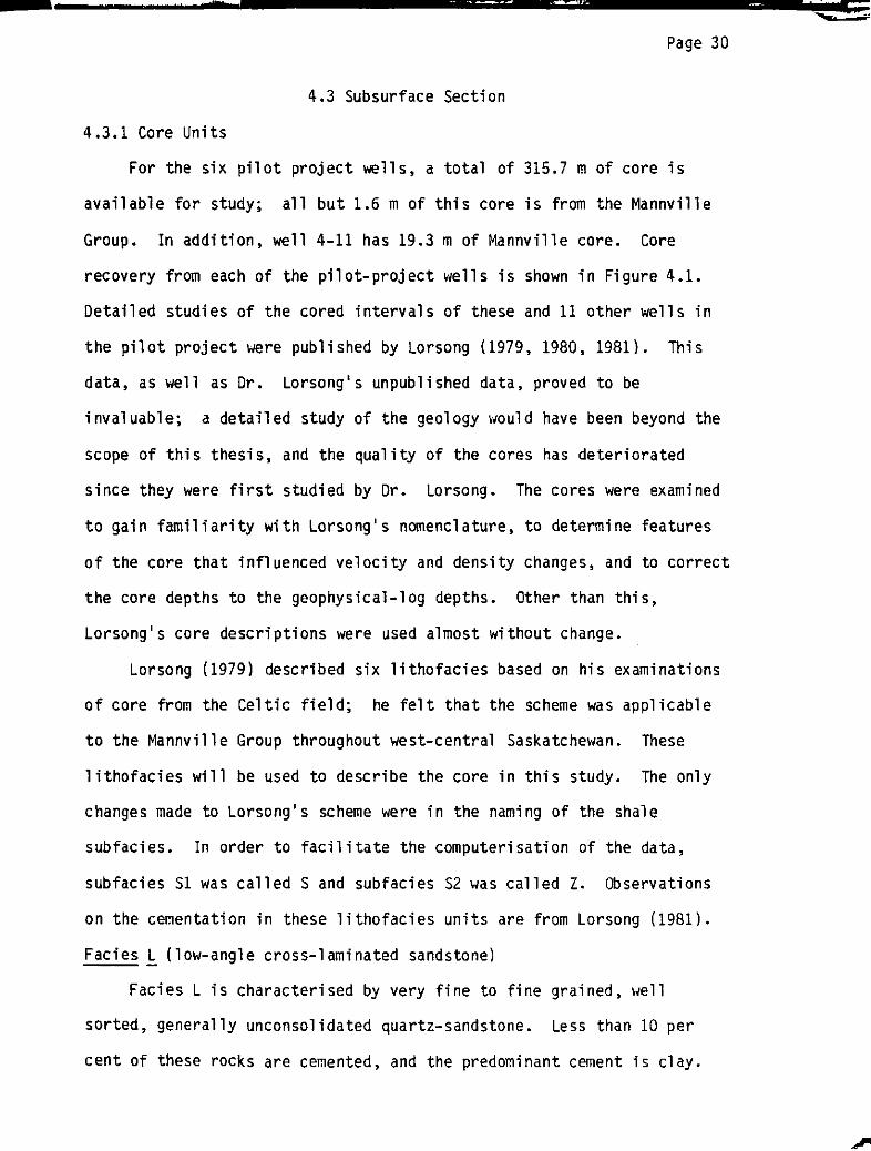
For the six pilot project wells, a total of 315.7 m of core is
available for study; all but 1.6 m of this core is from the Mannville
Group. In addition, well 4-11 has 19.3 m of Mannville core. Core
recovery from each of the pi 1 ot- proj ect vIe 11 sis shown in Fi gure 4.1.
Detailed studies of the cored intervals of these and 11 other we l l s in
the pilot project were published by Lorsong (1979, 1980, 1981). This
data, as well as Dr. Lorsong's unpublished data, proved to be
invaluable; a detailed study of the geology woul d have been beyond the
scope of this thesis, and the quality of the cores has deteriorated
since they were first studied by Dr. Lorsong. The cores were examined
to gain familiarity with Lorsong's nomenclature, to determine features
of the core that influenced velocity and density changes, and to correct
the core depths to the geophysical-log depths. Other than this,
Lorsong's core descriptions were used almost without change.
Lorsong (1979) described six lithofacies based on his examinations
of core from the Celtic field; he felt that the scheme was applicable
to the Mannville Group throughout west-central Saskatchewan. These
lithofacies will be used to describe the core in this study. The only
changes made to Lorsong's scheme were in the naming of the shale
subfacies. In order to facilitate the computerisation of the data,
subfacies Sl was called Sand subfacies S2 was called Z. Observations
on the cementation in these lithofacies units are from Lorsong (1981).
Facies � (low-angle cross-laminated sandstone)
Facies L is characterised by very fine to fine grained, well
sorted, generally unconsolidated quartz-sandstone. Less than 10 per
cent of these rocks are cemented, and the predominant cement is clay.

Page 31
Oil production in the Celtic field is almost exclusively from facies L
sand-bodies.
Facies T (trough cross-laminated sandstone)
Facies T is characterised by very fine to fine grained, quartz
sandstone that is moderately well sorted. small amounts of silt and
clay may be present. In the pilot area, more than 60 per cent of these
rocks are cemented, predominantly by clay and with lesser amounts of
calcite. For this reason, oil is seldom produced from facies T
sand-bodies.
Facies M (massive sandstone)
Facies M sandstones are fine to medium grained, moderately to
poorly sorted, and contain substantial quantities of silt and clay.
About half of these units are cemented, commonly by clay, less commonly
by calcite or iron-bearing carbonates. Facies M sand bodies are poor
oil-producers.
Facies B (bioturbated sandstone and shale)
Faci es B is made up of very fi ne to fi ne grai ned, we 11- sorted
sandstones and interbedded shale. About 20 per cent of these rocks are
cemented. Clay is the most common cement, followed by calcite, and then
by iron-bearing carbonates.
Facies 5 (shale)
Facies 5 consists of subfacies 5 and subfacies Z. Subfacies S is
characterised by massive intervals of shale and is never cemented.
Subfacies Z consists of massive shale that is similar, but has numerous
silty laminae. Less than one per cent of subfacies Z units are
cemented.
Facies C (coal)
Facies C is made up of thin beds of lignite and carbonaceous shale.

Page 32
Cementation does not occur in this lithofacies.
In order to relate the geology seen in the cores to the synthetic
seismograms, the core units must be compared to their response on the
geophysical logs and, when discrepancies occur, the thicknesses of the
core units must be corrected. Poor recovery of core is most common in
soft formations and at the ends of the core barrels. The core units
were fitted onto the velocity logs using coals, cemented zones, and oil
saturated sands as acoustic markers. Resistivity, density, natural
gamma, and caliper logs were used for additional checks during this
process.
The core-to-log correlation procedure resulted in subsurface
geology that is somewhat different from that described solely on the
basis of cores (as shown in Lorsong, 1980). In particular, it was
necessary to shift the lithofacies boundaries in well 2D8 up by
approximately 6 m in order to correlate the cores and logs. Other
differences were due to the incomplete recovery of coals, shales, and
oil saturated sands.
4.3.2 Geophysical-Log Marker-Beds
The complete suite of geophysical logs was used to pick
stratigraphic marker beds in the seven wells, and to make certain that
these picks \"iere consistent in all of the we l l s , Interpreted
geophysical-logs for these wells were available, but the way in which
the stratigraphic markers were defined and named, and the portion of the
well logs examined varied among the sources and even among the wells
from anyone source. Lorsong (1980) separated the cored intervals of
the logs into formations based on his detailed core examinations. The
well records of Mobil Oil Canada, Ltd. provided markers for the tops of

Page 33
the Second White-Speckled Shale and the Mannville formations. The
Saskatchewan Department of Mineral Resources consistently picked the top
of the Lower Colorado Subgroup, the top and base of the St. Walburg
Sandstone, the top of the Mannville Group, and the tops of the Mannville
sand bodies. White and von Osinski (1977) showed the Mannville sand
horizons present in well 4-11. Simpson (1981) gave an interpreted
cross-section of the Colorado Group near the Celtic field.
Within the Mannville Group, the formation boundaries described by
Lorsong (1981) were used whenever possible but, because the log-to-core
correlations had already been completed (see section 4.3.1), Lorsong's
core units could not always be related directly to the geophysical logs.
Moreover, the entire Mannville section was not available in anyone
cored interval. However, by extrapolating the information from well to
well, formation markers from the top of the Rex formation to the top of
the Colony formation (top of the Mannville Group) could be chosen.
These markers were compared with those of Mobil Oil Canada, Ltd. and
those of the Saskatchewan Department of Mineral Resources. Once the
preliminary interpretation of the logs in each well had been completed,
a cross-section through these wells was constructed to ensure that the
formation boundaries chosen were consistent. Horizons that proved to be
characteristic markers through the cross-section were: 1) a cemented
zone of high velocity and density in the Rex formation, 2) a cemented
zone of high velocity and density in the G.P. formation, 3) a cemented
zone of high velocity and density at the bottom of the Waseca formation
(except in well 202), 4) a coal bed of low density near the middle of
the McLaren formation, and 5) a large natural gamma anomaly at the base
of the Colony formation. Also, the oil-saturated sand-bodies were good
markers on the resistivity curves, and were visible on the acoustic and

........
Page 34
density logs.
During this correlation process it became obvious that the core
units in well 208 had been placed too deeply. The relative positions of
the lithofacies units were adjusted; this required shifting of the
formation boundaries chosen by Lorsong.
Once the formation boundaries within the Mannville had been
checked, an attempt was made to apply the lithofacies correlations made
by Lorsong (1980). This attempt met with little success because some of
the lithofacies units had been altered during the log-to-core
correlation, and because of the shift in the lithofacies units of well
208. Only the major sand beds, such as M2, W6, W4, W3, WI, S3, S2, and
Gl were named, and these cannot always be directly linked to the sand
beds of Lorsong (1980). A cross-section showing the core and log data
for the Mannville portion of the pilot-project wells is shown in Figure
4.5 (in pocket).
The Colorado Group stratigraphic markers were chosen based on the
well records of the Saskatchewan Department of Mineral Resources, the
well records of r40bil Oil Canada, Ltd., and the cross-sections published
by Simpson (1981). Within the Colorado Group, it was possible to
consistently pick the following markers: the base of the St. Walburg
Sandstone, the top of the St. Walburg Sandstone, the top of the Lower
Colorado Subgroup (base of the Second White-Speckled Shale), the top of
the Second White-Speckled Shale, and the top of the Colorado Group (base
of the Montana Group). As in the Mannville Group, the character of the
geophysical-log markers vas compared to be sure that they were
consistent from well to well. Figure 4.6 shows the stratigraphic marker
beds that were pi eked for we 11 202.
Well 4-11 was interpreted last because its log suite was not as

Page 35
DENSITY VELOCITY
KG/CUBIC METRE150.00 200.00
METRES/S
30.00
_10250.00
-uPPER ORIF'T
-------------MIDOLE ORIF'T
------------LO\.lER DRIFT
-----------MONfANA GROUP
crop OF LEA PARK FM.)
COLORADO GROUP
-------__ 2NO-\.IHI re: SPECKLED SH.-- i... COLORADO GROUP
__________MANNVILLE GROUP
-----------MCL ..\REN FM.
...::::;;::::-=--- - - -- --
-.Jo,-- - -
(J1
o
o
o
_________wASECA FM .
__________SPARKy F!'1.
__________ GENERAL PETROLEUMS FM.
_________ �EX FM.
Figure 4.6 -
Stratigraphic marker-beds for well 2D2·

Page 36
extensive as the others, its cored section was of poor quality, and its
logs were non-metric. Picking of the marker beds for well 4-11 by using
the now well-defined marker-beds of the other six wells resulted in log
interpretations that were consistent for all seven wells. The geology
in well 4-11 is different from that of the pilot project wells; a thick
shale interval is present in the Sparky formation and the Waseca
formation is reduced in thickness. The formation boundaries, and the
core and log data within the Mannville section of well 4-11 are shown in
Figure 4.7 (in pocket). This can be compared to the cross-section
through the pilot-project wells in Figure 4.5.
4.3.3 Properties of the Surficial Layers
Surface casing in the boreholes resulted in an absence of
geophysical-log data from the surface to depths of between 89 to 124 m,
depending on the depth of casing in the well. Although the
unconsolidated and weathered surficial-layers are thin and far removed
from the zone of interest, they exert a proportionately larger influence
on the seismic energy than would be expected. Velocities in these zones
are low, and the propagating waveform spends a relatively longer period
of time in these layers. Large velocity and density variations, often
due to gas content, are characteristic of the surficial layers, and as a
result, strong multiple reflections can occur. Moreover, unconsolidated
and shallow sequences are highly absorptive.
Information about the rocks within the cased sections of the
boreholes was inferred from geophysical logs and descriptions of
cuttings from shallow wells. Eleven shallow wells surrounding the pilot
project were chosen for this purpose; five are Saskatchewan Research
Council stratigraphic testholes and six are wells drilled under a

Page 37
Saskatchewan Department of Agriculture farm-improvement program. These
eleven wells were used to construct three cross-sections through the
area of the Celtic field. These lines of the sections did not pass
directly through the pilot project, and so, perpendicular projections
from the line of section and onto the location of well 2B8 were used to
locate the point closest to the centre of the pilot project. The
cross-section and well locations relative to the pilot project are shown
in Figure 4.8.
When the cross-sections were completed, the results indicated that
four distinct surficial layers should be present in the pilot project.
These were described (from the surface downward) in the cuttings as: 1)
a brown, sandy to silty till, 2) a well consolidated, grey till, 3) sand
and gravel interbedded with grey till, and 4) a grey, bedrock shale--the
Lea Park Formation. B. Schriener (personal communication, 1981)
suggested that unit 1 is the Battleford Formation, and that unit 2 is
the Floral Formation. However, as Quaternary stratigraphy is not within
the scope of this thesis and because an origin of the sediments is not
meant to be implied, units 1, 2, and 3 will be simply referred to as the
upper drift, middle drift, and lower drift. Unit 4 was interpreted as
the top of the Lea Park Formation.
The elevations of the tops of the three lower layers, at the points
closest to the center of the pilot project, were noted for each of the
three cross-sections. The thickness of each layer was calculated for
all three of the cross-sections; these were then averaged to obtain a
representative thickness of each layer in the study area.
Velocity and density values for the surface layers were difficult
to obtain and so they were modified from published values for similar
1 i thotypes (Burke, 1968; Chri sti ansen, 1970; Pa tterson, 1964). These

ASASKATCHEWAN RESEARCH COUNCIL
STRATIGRAPHIC TESTHOLE
_�TP53
R21 R20
AI
R23R24 R22
Figure 4.8 - Location map for the shallow wells used to infer information about the surficial layers in
the study area.
A
Tp 51
NORTH
SASKATCHEWAN
RIVER
MILES
o 5 10
"
II'
i I
o 5 10
KILOMETRES
SASKATCHEWAN DEPARTMENT OF
AGRICULTURE BOREHOLE
A A LI N E OF SECTION
•
I
-0
Q.I
�W
00
(:

Page 39
modifications were based on discussions with geophysicists with
long-term Saskatchewan experience (Gendzwill and Hajnal, personal
communication, 1982). The average thickness, velocity, and density for
each surface layer are given in Table 4.3. These values are constant
for all of the wells used in this study and are contained in a data file
called GANCEL.DAT, which is used as input to the synthetic seismogram
program as well as to several of the plotting routines.
The depths of all of the stratigraphic marker beds, from the
surface to the bottom of the hole, for each of the seven wells are shown
in Table 4.4. A data file containing these 15 depths was constructed
for each of the wells. The files are called PIX.DAT (for example
PIX2B8.DAT) and are used as input to plotting programs and to the
synthetic seismogram program.
4.4 Core Analyses
The measured rock properties of porosity, permeability, clay
content, and oil saturation, as well as the observed type of cementation
in the rock, affect the acoustic properties of the rock and also
determine its potential for oil production. Analyses of porosity, oil
saturation, and permeability to air were performed on the
freshly-recovered core of the pilot-project wells by Core
Laboratories--Canada Ltd. Porosity and the fraction of pore volume
saturated by oil were from Dean Stark analysis, and the permeability to
air was determined by small plug analysis. Details of the methods can
be found in the API Recommended Practice for Core-Analysis Procedure
(1960). The amount and type of cementation, and the per cent of clay
content in the rocks were based on core studies (Lorsong, 1981;
Lorsong, unpublished data).

I
\. (--
TABLE 4.3. SURFICIAL-GEOLOGY DATA
UNIT DESCRIPTION DEPTH·TO TOP THICKNESS VELOCITY DENSITY
lower dri ft brown, sandy to 0.0 m 9.8 m 1219 m/s 2192 kg/cu m
sil ty till
middle drift well consolidated 9.8m 20.1 m 1829 m/s 2072 kg/cu m
grey ti 11
upper drift sand and gravel 29.9 m 16.8 m 2134 m/s 2100 kg/cu m
interbedded with
grey till
Lea Park Fm. grey shale 46.7 m variable 1890 m/s 2100 kg/cu m
( bedrock) (at top) (at top)
""0
j;U
c.o
t1>
�
o

Page 41
TABLE 4.4. STRATIGRAPHIC MARKER-BED DEPTHS
4B2 202 402 2B8 4B8 208 4-11
(m) (m) (m) (m) (m) (m) ( m)
upper drift 0.0 0.0 0.0 0.0 0.0 0.0 0.0
middle drift 9.8 9.8 9.8 9.8 9.8 9.8 9.8
lower drift 29.9 29.9 29.9 29.9 29.9 29.9 29.9
Lea Park Fm. 46.7 46.7 46.7 46.7 46.7 46.7 46.7
U. Colorado 234.0 238.0 244.0 243.3 260.9 245.0 264.3
Subgroup
Second White- 262.5 267.0 272.5 277 .3 289.5 301.5 293.3
Speckled Shale
L. Colorado 273.5 273.3 278.6 283.0 295.5 308.0 299.7
Subgroup
top St. Walburg 307.2 311.6 314.8 320.6 333.1 346.2 336.9
Sandstone
base St. Walburg 321.3 326.5 329.1 335.8 349.0 361.0 352.1
Sandstone
Mannvi1l e Group 402.2 404.5 409.5 414.0 427.5 443.3 425.5
McLaren fm. 417.2 420.1 428.7 428.2 440.9 455.2 434.4
Waseca fm. 434.0 437.0 441.4 447.4 459.8 474.7 454.3
Sparky fm. 452.9 453.8 460.9 467.1 479.0 496.1 465.2
G.P. fm. 472.0 474.4 478.0 483.0 496.2 511. 7 497.6
Rex fm. 482.3 484.3 488.4 492.9 506.5 523.2 506.8

Page 42
When several values of core analyses were available for a bed (for
example W6), the means were calculated to give representative values of
porosity, permeability, and oil saturation for the entire bed. An
example sheet of core analysis results is shown in Figure 4.9. In
addition to the analyses shown in Figure 4.9, Core Lab determined the
lithotype of each sample by visual examination. The first step in
reducing the data was to allocate the depth intervals (each of about 20
cm in thickness) used for the Oean Stark analysis to the lithofacies bed
to which they belonged. In wells 4B2, 202, 402, and 208 this had
already been done (Lorsong, unpublished data). In the remaining two
pilot-project wells this was done by comparing the Core Lab lithotype
descriptions and depths to the detailed core-descriptions (Lorsong,
unpublished data).
The core analyses were almost always made in the sandier, more
oil-saturated intervals of the core. For this reason, analyses in beds
of uncemented facies L were generally available, data from beds of
facies T and M were less common, data from facies B beds were biased
toward the sandy intervals, and analyses from cemented intervals or beds
of facies S, Z, and C were nonexistent. Furthermore, permeability
measurements were not made in every interval. In beds where analyses
was not available, data were extrapolated from values in other beds of
the same lithofacies. If this was not possible, published measurements
of rock properties were used as a guide for selecting a value.
Porosities of shales and coals were found in Greensmith (1978, p. 102)
and Karr (1978 p. 156), respectively. Permeabi1ities of sands,
sandstones, and shales are available in Pettijohn (1975, p. 78) and
Blatt, Middleton, and Murray (1972, p. 347). The range of porosities,
oil saturations, and permeabi1ities of cemented lithofacies L sandstones

I
(:
DEAN·STARK ANAL YSIS SMALL PLUG ANALYSIS
Sa tur ill ion
Bulk Mass Fraction Fraction or Pore VolumftPerrneabill ty
Boyle'sGrain
Sal,,�eDepth m Porosity (Calculaled) law
Nwn er Mellin [m] Rep.
I(Calculaled)
to Air Helium Oemicy
Oil Willor OilTOlal Millidarcys Porosity kg/m3Waler
CORE NO. 1 426.00 m - 432.00 m (REG. 4.40 m) (3 BOXES)
426.00-27.46 1.46
1 427.46-27.74 0.28 0.076 0.094 0.351' 0.447 0.553
427.74-28.46 0.72
2 428.46-28.68 0.22 0.043 0.091 0.290 0.321 0.679
3 428.68-28.93 0.25 0.061 0.098 0.333 0.384.
0.616
4 420.93-29.23 0.30 0.062 0.074 0.294 0.456 d.544
5 429.23-29.42 O. 19 0.068 0.063 0.285 0.519 0.481
6 429.42-29.68 0.26 0.030 0.076 0.238 0.283 0.717
7 429.68-29.93 0.25 0.099 0.074 0.356 0.572 0.428
8 429.93-30.14 0.21 0.081 0.072 0.323 0.529 0.471
9 430.14-30.40 0.26 0.059 0.092 0.320 0.391 0.609
430.40-32.00 1.60
CORE NO. 2 432.00 m - 438.00 m (REC. 5.20 m) , (4 BOXES)432.00-32.32 0.32
10 432.32-32.49 0.17 0.039 0.026 0.155 0'.600 0.400
11 432.49-32.79 0.30 0.033 0.049 0.191 0.402 0.598
12 432.79-33.12 0.33 0.089 0.098 0.378 0.476 0.524
433.12-33.97 0.85
13 433.97-34.30 0.33.
O. 101 0.048 0.316 0.678 0.522
DB 1 434.30-34.39 0.09 - - - - - 2180. 0.�46 2620
14 434.39-34.71 0.32 0.093 0.050 0.306 0.650 0.350
15 434.71-35.03 0.32 0.096 0.055 0.320 0.636 0.364
16 435.03-35.27 0.24 0.043 0.055 0.223 0.439 0.561
17 435.27-35.48 0.21 0.044 0.088 0.286 0.333 0.667 - . - - '0
I»
(Q
Figure 4.9 -
Example sheet of core-analysis results. II)
.J:!oW

Page 44
are given in Lorsong (1981).
The amount and type of cementation was determined from the core
descriptions (Lorsong, unpublished data). Three types of cement can be
distinguished in the cores: clay, calcite, and carbonate (mainly iron
carbonate) (Lorsong, 1981). The amount of cementation varies from
complete, to partial, to nodular (calcite and carbonate only). Also, a
mixture of more than one type of cement was sometimes noted.
Cementation often does not extend through the entire lithofacies bed.
Because it is such an important factor in the acoustic properties of the
rock, lithofacies beds were subdivided so that the type and habit of
cementation within each bed was constant.
Average clay content of each lithofacies type was based on
discussions with Dr. Lorsong (personal communication, 1982). A
constant, average value of clay content as a percentage of rock volume
for each lithofacies was used. If a bed was clay cemented, the amount
of clay was calculated by assuming that the decrease in porosity of the
rock vas entirely due to increased clay-content.
Data files called CA.DAT (for example CA2D2.DAT) were used to store
the core data for each well. The contents of these CA.DAT files are
presented in Appendix A. The files include the unit number, lithofacies
type, bed, thickness, and depth (to the top) of each unit. The next
column is a code for the cement type; then porosity, oil saturation,
permeability, and clay content values follow. CA.DAT files are used as
input to plotting routines LOGGRF and CELGRF. The LOGGRF plotting
routine was written to allow easy comparison of the velocity and density
logs to the oil saturation and cement type of each lithofacies bed.
LOGGRF was used to plot the data for each well in the cross-section of
Figure 4.5 (a listing of this program can be found in Appendix B). A

Page 45
portion of the program CELGRF plots all of the core analysis data, but
as this program was mainly used to plot the synthetic-seismogram data,
CELGRF will be discussed in section 5.1. In both programs, core data
are plotted at the same scale as the log data and synthetic seismograms;
this allows for easy comparison.
4.5 Q values
Absorption of seismic energy in the Cretaceous sequence of the
study area is likely to be a problem because of the shallow occurrence
and unconsolidated nature of the beds. The absorptive properties of
rocks are specified by many different units of measure, but the most
commonly used measures are the absorption coefficient � and the specific
attenuation factor, or quality factor, Q (Johnston and Toksoz, 1981).
The quantities are related as follows:
1
= ---------
Q 8.686-rr
Where 0<. is measured in dB/A.
Q is an intrinsic property of the rock. It defined as the ratio of
2�times the peak elastic energy per cycle of a harmonic wave, to the
energy dissipated in one cycle of the harmonic wave (Ganley, 1979). Q
is inversely related to absorption; as absorption increases, Q
decreases. In the present study, the absorptive characteristics of each
layer of the depth model used to construct the synthetic seismogram were
spec i fi ed by Q.
Measurements of the absorptive behavior of the rocks in the study
area were not available; in consequence, the Q values attributed to

Page 46
these rocks were modified from values published for similar types of
rocks in other areas. In order to be directly applicable to the study
area, the absorption measurements must be made � situ, at seismic
frequencies, and in shallow, unconsolidated sedimentary-rocks.
Measurements of this type are relatively rare, but a summary of the
published values that fulfill most of these criteria is presented in
Table 4.5.
Widely recognized, fundamental trends in the absorptive behavior of
rocks were used to modify the published values of Q presented in Table
4.5, so that they would better suit the geologic environment of the
study area. These fundamental trends are reviewed briefly in the
remainder of this paragraph. Johnston et al •
--
(1979) recognized the
following relationships: 1) Q increases with increasing differential
pressure (or, in most cases, with depth), 2) Q is higher for dry rocks
than for saturated rocks, and 3) Q values obtained by ultrasonic methods
are lower than those obtained by lower frequency techniques. Hamilton
(1972) related attenuation to the shear, or rigidity, modulus; rocks
that are more rigid (that is, cemented or less porous rocks) should have
higher Q values. Hauge (1981) noted that as the percentage of sand
content in sedimentary rocks increased, the Q of the rocks decreased.
In the present study, the subsurface was separated into five zones
for the purpose of allocating Q values. The three drift layers were
each given a different Q because of their different lithotypes and
degrees of consolidation. The Colorado Group is predominantly shale,
therefore, it was treated as one unit. The interbedded sands and shales
of the Mannville Group constitute the last unit. The Q values chosen
for these units are shown in Figure 4.10. The values for all of the
units, except the Colorado Group, are constant. Because the Colorado
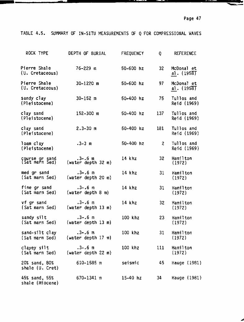
Page 47
TABLE 4.5. SUMMARY OF IN-SITU MEASUREMENTS OF Q FOR COMPRESSIONAL WAVES
ROCK TYPE DEPTH OF BURIAL FREQUENCY Q REFERENCE
Pierre Shale 76-229 m 50-600 hz 32 McDonal et
(U. Cretaceous) ai. (1951IT
Pierre Shale 30-1220 m 50-600 hz 97 McDonal et
(U. Cretaceous) al. (1951IT
sandy clay 30-152 m 50-400 hz 75 Tullos and
(Pleistocene) Reid (1969)
clay sand 152-300 m 50-400 hz 137 Tullos and
(Pleistocene) Rei d (1969)
clay sand 2.3-30 m 50-400 hz 181 Tull os and
(Pleistocene) Reid (1969)
loam clay .3-3 m 50-400 hz 2 Tull os and
(Pleistocene) Rei d (1969)
roursegr sand .3-.6 m 14 khz 32 Hamilton
Sat marn Sed) (water depth 32 m) (1972)
med gr sand .3-.6 m 14 khz 31 Hamilton
(Sat marn Sed) (water depth 20 m) (1972)
fine gr sand .3-.6 m 14 khz 31 Hamilton
(Sat marn Sed) (water depth 8 m) (1972)
vf gr sand .3-.6 m 14 khz 32 Hamilton
(Sat marn Sed) (water depth 13 m) (1972 )
sandy si 1 t .3-.6 m 100 khz 23 Hamilton
(Sat marn Sed) (water depth 13 m) (1972 )
sand-silt clay .3-.6 m 100 khz 31 Hamilton
(Sat marn Sed) (water depth 17 m) (1972 )
cl ayey si 1 t .3-.6 m 100 khz 111 Hami 1 ton
(Sat marn Sed) (water depth 22 m) (1972)
20% sand, 80% 610-1585 m seismic 45 Hauge (1981 )
shale (U. Cret)
45% sand, 55% 670-1341 m 15-40 hz 34 Hauge (1981)
shal e (r4i ocene)

·
o
o
o
o·
o
o
'"
o·
o
o
N
o
o·
o
o
C
rrI
"lJN
-1'"
::J:?o
_0
:z
3""
rrl°-10:::00
rrl°(/'J
·
o
o
..
o
o·
a
o
·
c»
o
(II
o
o
Q40.00 80.00
--UPPER DRrFT
------------ - ----_"IODLE DRIFT
STRATIGRAPHIC
MARKER BEDS
-----------LOVER DRIFT
---------__MONTANA GROUP
(TOP OF LEA PARK FM.)
--u. COLORADO GROUP
--2NO-�JTE5PECKbED
SH.
--L. COLORADO GRO I'
--TOP ST. WALBURG SST.
--8AS£ ST. WALBURG SST-
�--------------�---MANNvrLLE GROUP
- - MCLAREN Fn-
--SPARKY F'M.
·-G�£RAL PETROLEUMS fM.
--REX FM.
·
o
____CL."--- . _
Figure 4.10 - Q values used in the study area.
Page 48

Page 49
Group unit is so thick, the Q within this unit was increased linearly
from a reasonable value at its shallowest depth to a reasonable value at
its deepest depth.
The choice of Q, or the way in which Q varies within the units
cannot be rigorously defended. In section 5.3.3 it will be shown that
(within reason) it is the average value of Q, rather than the shape of
the Q curve that affects the lower portions of the synthetic seismogram.
If real seismic data were available, an attempt could be made to model
the input Q values until the shape of the synthetic seismogram
approximated the shape of the seismic traces. This should be done with
traces plotted without gain control.

Page 50
CHAPTER FIVE
GEOPHYSICAL PROCESSING AND ANALYSIS
5.1 Synthetic Seismograms
The method of synthetic-seismogram synthesis used in this thesis
was described in Ganley (1979, 1981). In this method, the communication
theory approach to synthetic-seismogram construction is modified to
include the effects of absorption and dispersion. Historical
developments in the expression of seismic wave propagation through
layered media by communication theory were reviewed by Robinson and
Treitel (1977). The absorption model used in the program for
synthetic-seismogram construction is that of the exponential decay of
amplitude as a function of distance. Absorption is mathematically
introduced by allowing the elastic modulus in the elastic-wave equation
to be a complex function of frequency. As a result, the velocity and
wavenumber, as well as the reflection and transmission coefficients
become complex functions of frequency. Dispersion is introduced by
equations derived by Futterman (1962), which relate dispersion to
absorption.
Futterman (1962) demonstrated that if a linear theory of wave
propagation is assumed (that is, if the principle of superposition is
valid), and the absorption coefficient o<{w) is strictly linear vi th
frequency over the range of measurement (that is, Q is constant over
this range), then the presence of dispersion is a necessary consequence
of absorption and is, in fact, determined by it. Using the condition of
causality, which states that a signal will not be detected at an
apparatus until sufficient time has passed for it to arrive there,
Futterman related dispersion to absorption and calculated the dispersion

Page 51
for three absorption functions. Ganley defined his absorption and
dispersion relations by using Futterman's third absorption-dispersion
pair.
For typical earth cases (Q greater than 20) and in the frequency
range used for seismic exploration, dispersion is small but measurable
(Toksoz and Johnston, 1981). Futterman (1962) demonstrated how
dispersion caused a propagating pulse to broaden, decrease in amplitude,
and become asymmetrical with increasing time. As a result of
dispersion, the higher-frequency components of the wave travel with a
higher phase velocity; the front of the pulse becomes sharper and the
pulse has a definite arrival time. However, as time passes, absorption
begins to reduce the high frequency content of the wavelet and the
effects of dispersion become less pronounced.
Ganley's original synthetic-seismogram program was tested on the
computer facilities available at the University of Saskatchewan by
computing and plotting the surface trace of the example synthetic
seismogram shown in Ganley (1981). Ganley (1981) described two methods
of synthetic seismogram synthesis. The program used in the present
study employs the ratio approach, which calculates a synthetic
seismogram only at the surface layer. It also has the capability to
calculate the surface synthetic-seismogram for a buried source.
Modifications to this program were made to suit the present study. The
original format required an input thickness, Q value, density, and phase
velocity for each depth layer of the model earth. This format was
preserved for the layers within the cased portions of the wells, but was
changed for the portions of the we l l \�here geophysical logs supplied the
velocity and density data. The synthetic-seismogram program is called
SYNCEL; it is listed in Appendix B.

Page 52
A downgoing spike is used as the energy source in the original
program. To give an additional choice of wavelet shape a subroutine
called PULSE vas written. This subroutine generates Ricker wavelets
(Ricker,1953a). Although the viscoelastic model on which the Ricker
wavelet is based may not be realistic, the concept of this wavelet has
been extensively used in exploration seismology (Toksoz and Johnston,
1981). With PULSE, four different types of Ricker wavelets, of variable
peak frequency, can be computed. Of the four, only the direct phase or
velocity-type Ricker-wavelet was used in this study. PULSE also
includes equations to calculate the phase and amplitude spectra of the
wavelet.
The method of constructing the synthetic sei smograms was uniform
during this study. Due to dispersion, the phase velocity and Q values
will vary with frequency. In the present study, the input Q values and
phase velocities were at frequencies of 100 hz (as in Ganley, 1981).
The low frequency cut-off (as required by Futterman) was at .0017810724
hz,
The synthetic seismograms are calculated as a continuous function
of frequency. In order to avoid the effects of aliasing in the time
domain when using a discrete Fourier-transform, sampling in the
frequency domain must be at a small enough spacing, Af, that for times
greater than Tn=1/cif=2lT/ciw, the amplitude of the synthetic seismogram is
negligibly small (Ganley, 1981). Ganley has found that choosing Tn to
be four to eight times the two-way time of the model is usually
adequate. In the present study, Af was chosen so that Tn is
approximately eight times the two-way time of the model. Inspection of
the calculated synthetic-seismograms verified that, at times approaching
Tn (4.096 s), the amplitudes are indeed negligibly small. The Fourier

,-
1_"- .-.- -
_ __ __ � __
Page 53
transforms of the synthetic seismograms were evaluated by 2049 discrete
frequency-values between 0 and 500 hz, inclusive. In the time domain,
4096 points were calculated, at a time interval of 1 ms.
In order to perform the discrete Fourier-transform, the data must
be band limited and the contributions of frequencies beyond a maximum
frequency must be eliminated. To reduce any undesirable effects, a
sut.tervor-th low-pass fil ter was used to reduce the ampl i tudes of
frequencies beyond the cut-off frequency (Ganley, 1981). The amplitude
response of this filter is 3 decibels down (29.2 per cent reduced from
the maximum amplitude) at 250 hz and 72 decibels down (99.9 per cent
reduced from the maximum amplitude) at 500 hz. The time domain
synthetic now approximates the synthetic that would be recorded through
an anti-alias filter with the characteristics of the low-pass
Butterworth-filter.
A computer program called CELGRF was ��itten to plot the synthetic
seismograms and those properties of the subsurface that could affect the
seismic response. The plots include the shape and normalized amplitude
spectrum of the Ricker wavelet source (if used); the synthetic
seismogram; the Q, velocity, and density values; the stratigraphic
markers; and the core properties of porosity, permeability, oil
saturation, clay content, cement type, and lithofacies type. The rock
properties and synthetic seismograms are plotted at the same scale and
as closely together as possible, to facilitate the recognition of cause
and effect relationships between the two. The rock properties are
plotted versus depth and the seismograms are plotted versus both time
and depth. Examples of plots produced by CELGRF are shown in Figures
5.2 through 5.6, 5.8 through 5.13, 5.17, 5.19 through 5.25, 5.30 through
5.37,5.44 through 5.50, 5.58, 6.1, 6.6, and 6.8 through 6.10.

,-
" ..-.- .
--- - - --
.
-,
Page 54
In order to compensate for the attenuating effects of absorption
and short-period multiples, and thus, provide more equal amplitude
levels from early to late events, a gain function may be included in the
synthetic-seismogram plotting-routine. The gain control is provided by
a power gain-function that computes the energy within sliding
time-windows and then applies a gain that is inversely proportional to
the energy in the time window (Sereda, 1978). Tests were made to
determine the optimum window length for the data in this study. The
best results were obtained by specifying a window length of 0.10 s.
It is sometimes desirable to plot the synthetic seismogram without
gain (a true-amplitude plot). For example, this was done in section
5.3.3 to study the attenuation effects of different Q values. When no
gain control is desired (that is, when the window length in CELGRF is
set to 0.0 s) the high amplitude, direct-wave arrival on the seismogram
is automatically muted. Muting of this arrival is also automatic when
the seismic source is buried.
5.2 Spectral Analysis
There is an interchangeability between a waveform as a function of
time, such as a seismic trace, and the spectra of the waveform that show
ampl i tude and phase as functi ons of frequency; liThe ampl i tude and phase
spectra, taken together, uniquely define their corresponding composite
wavefonn" (Anstey, 1965, p. 6) . Bath (1974) described several
advantages of thi s form of representati on. The fi rst is that, when
expressing a waveform as functions of frequency (spectral analysis) the
whole signal shape is used in the analYSiS, whereas the common time
domain measurements (such as displacement direction, maximum amplitude,
or onset time) are point measurements. Spectral analysis can,
Page 55
therefore, because of its style of presentation, yield more useful
information than time measurements. The second advantage is that, when
making comparisons of different records it is important to be sure that
exactly the same thing is compared in all cases. The frequency-domain
representation provides a unique check that the parameters being
compared are all referred to the same frequency value. Time domain
representations do not provide such reliable control.
Spectral analysis was performed for the Mannville sections of the
synthetic seismograms. These amplitude spectra provided a quantitative
measure of the changes in amplitude of the frequency components of the
propagating seismic energy in the zones of interest, as input parameters
to the synthetic seismogram were varied. The input parameters that were
varied will be described in the remaining sections of this chapter.
A spectral analysis program call SPECAN was used to calculate these
spectra. SPECAN is a generalized spectral-analysis program, employing
the efficient fast-Fourier-transform (Rielkoff, 1982). The program was
tested by computing the amplitude spectra of sinusoidal time-series. A
calcomp plotting routine was added to SPECAN; the amplitude values,
were first smoothed by the Hanning method (Titchkosky, 1968, p. 87) and
then were normalized and plotted. An example amplitude spectrum is
shown in Figure 5.7. The low amplitude of the spectrum from about 250
to 500 hz indicates a lack of energy beyond 250 hz. This is to be
expected because the Butterworth low-pass filter used in the synthetic
seismogram program severely filters frequencies above 250 hz.

,
-- •
_ ... M
�_�_
Page 56
5.3 Model Parameters
5.3.1 Introduction
Tests were made to determine the effect on the synthetic seismogram
of variation in the input parameters of the Q value, the depth of burial
of the source, the frequency content of the propagating wavelet, and the
subsurface geology in the zones of economic interest. Well 2B8 was
chosen as the subject of these tests because: 1) it is in the centre of
cross-section AA' (see Figure 4.1), 2) it is a typical example of the
representative and economically important geologic features of the six
pilot-project wel l s, 3) it has geophysical logs of good quality, and 4)
it has a very long cored- secti on, �Jhi ch i ncl udes most of the zone of
geologic modelling.
Although only one input parameter at a time was varied, and
although the parameters are discussed separately, it is critical to note
that it is the combined effect of all of the parameters that determines
the output. The testing was an iterative process, in which first one
parameter and then another was vari ed. Earl i er tests were often
returned to and run agai n wi th sl i ghtl y di fferent input parameters. In
order to point out the important synthetic seismogram responses, the
variations in the input parameter of subsurface geology are discussed
first.
The polarity convention used in this thesis is that a peak is a
deflection to the right. It is reflected from an interface in which a
layer of higher acoustic-impedance overlies a layer of lower
acoustic-impedance. A trough is a deflection to the left and results
from the opposite acoustic-impedance layering.

-" �
.. <
_-. .. � -
• - - �
Page 57
5.3.2 Geologie modelling
The responses of five beds of economic importance were studied by
comparing synthetic seismograms constructed with the beds unaltered and
altered. The five beds were not actually removed from the wells;
instead, their characteristic effects were edited from the velocity and
density logs. In Figure 5.1 the edits made for each of the six test
cases are shown. For example, when the response of the oil-saturated
sand-bed W6 is removed from the synthetic seismogram, the low velocity
and density signature of the oil-saturated sand must be removed by
increasing the velocity and density of the W6 zone to values similar to
that of the unsaturated, sha1ey sand-beds above and below; the
oil-saturated sand-bed is artificially shaled out. The seismograms used
for geologic modelling were constructed with the input parameters of an
impulse source, the Q curve shown in Figure 4.10, and a source burial of
29.9 m. The input parameters are summarized in Figure 5.2.
When the effects of all of the Waseca formation oil zones (that is,
W3, W4, and W6) are deleted from the input logs, the resulting
seismogram is as shown in Figure 5.3. The unmodified well logs and
their seismic response are shown in Figure 5.4. When comparing these
two synthetic seismograms, the most obvious difference between them is
that two low amplitude, high frequency peaks at about 0.42 s in Figure
5.4 are eliminated in Figure 5.3. Those waveforms appear to be
generated by the oil-saturated sands W6 and W3. To test this
hypothesis, the two main oil-zones, W6 and W3, were separately edited to
appear shaled out. When the effect of the oil-saturated sand in bed W6
was removed from the well logs, only the upper waveform disappeared from
the synthetic seismogram. This is illustrated in Figure 5.5. As is
shown in Figure 5.6, when the effect of the oil-saturated sand in bed W3

-� -_- - - - --�.....
.'
.............. ._,_
��-...-..... --._-A.-#._
DENS 1 TY
CELTIC 288 10 52 23 W3M
'1ELOCI TYCORE DATA
.-
...
8
;
�
...
<II
..
�
�
�
�2!
HlP �F C�AE
�Y:26.6 M
Q
'e:!
...C (CCI
�..., ca' _
�
! ....,
I .00II' caT l18li..
..
� 111M.)
I !.!MS'
�....,
�S lilli'
...
lllf!' CIII.._..
<II
g T IMTI
.c9 eMit �T el
"
I.c Tnm"
T I"TI
� .II1II,
1! ll"'l
.. a ...."
'"
... IU.•• aileQ
.... ,
�
:• l1li,
:g
8a 'WI'
� I L .....
Q
� • l1li,
..
Q
;'"
'"
.... ,
�..
'"
� a l1li'
8I U,'J
.c
...!!I 114' CIT
"
�unl CIILe
�<II
Z ",.'"
)110'
COLONT 1=;.;;._....;;c;�___;=:;;_....:;,;;.l6O;;.;..
.;;;;QO___;==-�FI1.
lTep I5F
HANNY [LLECROUP)
HCLAREN
fH •
WASECA
FH.
SPRRKY
FH.
� GAS ZONE, 2500 m/s
Page 58
.... McLAREN COAL ZONE, 2410 m/s
ZONE, 2500m/s
.... W3 ZONE. 2500m/s
WI ZONE, 2500m/s
Figure 5.1 -
Well-log zones edited for geologic modelling.

1
-0
s:»
c..o
I'D
0'1
\0
NUMBER OF POINTS REOUESTED IN SYNTHETIC TRACE = 4096
SAMPLE INTERVAL FOR SEISMOGRAM AND WAVELET (MS) = 1.
TYPE OF WAVELET = IMPULSE i THE DIRECT WAVE IS MUTED
BUTTERWORTH ANTI-ALIAS FILTER INCLUDED IN SYNTHETIC TRACE
POWER GA 1 N FUNCT I ON INCLUDED, WI NDOW LENGTH (S) = 0.10
WELL IS CASED TO A DEPTH (M) =:125·4
NUMBER OF CONSTANT VELOCITY LAYERS WITHIN CASED SECTION = 13.
RECEIVERS LOCATED AT TOP OF LAYER 1
DEPTH OF SOURCE BELOW RECEIVERS (M) =: 29.9
Figure 5.2 -
Summary of parameters used to construct synthetic seismograms for geologic modelling.
\.

...
o
<>
so
1"1
11 ...
--<'"
:r!'o
_0
Z
;]:<-11"10....
0
;UU1"10en
o
o
00.00 40.00 10.00
;, I I« « «
o
'"
o
o
o
CELTIC
DENSITY
KG/CUBIC METRE -'0'
0150.00 200.00 l50.00
o
o
...
o
o
o
oo
g
...
s
go
1"1
" ...
.......
:rD
-g:z:
;]:"1"10....
0
;uo1"10(IJ
�o
g
.
o
o
g
'"
o
g
'"
o
.,
o
o
288 10 W3M
.,
o
g
52 23
..
o
g
...
..
o
v
o
..
oo
g
..
o
"
o
..
o
v
g
VELOCITYSYNTHETIC STRATIGRAPHICSEISMOGRAM MARKER BEDS
METRES/S _'02 AMPLI TUDE _'02
010•00 10.00 50.00
?-6U.00-30.00 0.00 30.00
?rw'""'"
I« I I I «
0g ·-HIOOLE OftlflgL1 0
-lOWEft O�lrf
:� r.. ..
°? -HOH I AHA CRGUP
0
g tlOP 0' lEA PARK '".1o -.OS S
(; (; (;0 0 0
g g -"0' g
;;. ;;. ;;.0 0 0
., g -.15' go.
... ... ..
0g
0
0 0
., g -·lO' 0
0 0
0 0 0
1"1 1"1 1"1
11 ... 11" 11 ...
-I" .... ..
-;, �-l--U. rOlORAOO C,ROUl':r? :r?
0
_g -.as s _g_o
:z: :z: z
1 �lND;:III.·mD5P��GW;D�".
;]:'"
�g �g1"10....
0..... .....
�g:Uo
:ug..,0 - .30 , �i-lop
51. WAlBURG SSI.(IJ (IJ
... ..
�-BAS[ SI. WALBURG 551.
... ...
�0 0
0 g s0
- .35 S
il-L �l'"g•
rm...."'_�
-HClAR[1f rH.
A
� -WASfCA rH.
0
o "'�PAR'" rH.
-CU[IUl PUROlfUHS rH.
H � H4S S
.>� I-RU 'H.
0
0
0
..
<eo
o
.,
.,
Figure 5.3 - Well logs and seismogram when the Waseca fm. oil-zones are edited to appear shaled out.
I
"'0
AI
to
(J)
m
o

CELTIC
a DENSITY
0 ItG/CU8lC "EIRE .to'
0°.00 40.00 .0.00 0150.00 100.00 ISO. 00
.. ..0 ..
... ...
0 0
.. g..
0 i0
.. g0
;;. ;;... 0
g g
.. ...
.. 00 ..
g g0 0
'" '"""ON -UN
-4" .....
x? x?0
..-g_0
:z ::z
�g �g-4. ....
�g �gII> flO
...
t...
0
g g
..
g0
0
g g
.. ...
.. ..
.. ..
g g
... ...
0 .... C>
.. <.0 0
'" ..
... ..
.. ..
g g
288 10 52 23 W3MSYNTHETICSEISMOGRAM
AMPll ruor .,0'
0-'0.00 -30·00 0.00 30.00
. I' • •
I' I
g
�..
g
Figure 5.4 - Unmodified well-logs and resulting synthetic seismogram.
VELOCITY
METRESIS ·to'
0'0.00 lO.OO SO. 00
I' • , ,
gI
z
\.
..
C>
g
g
g
;;o
g
'"
D
..
go
'"
-UN.....
:.:0
-g
:x��o::u'",gflO
tlo
g
...
g
g
gg
..
D
g I,.-.OS S
ig.-.,oc
lit
..
g 1--.15 I
...
g
g .-.�o S
0
....
""ON
.... ..
x?
_g.-.asc::z
:XU.... 0
...0
::ugc: .-.JO C
tl0
g
t-·JSC
...
00
g
i- ... c
...
...
C>
g
g .-.45 S
<.0
STRATIGRAPHICMARKER BEDS
? -"r£1I PIlin
81-nI00l.[ PIIIH
�.-lOUfIl Oilin
lit
? -_tall' ell_
g nor or lU nil!! 'n.1
gg
ig
8g
00
PI
""0'"
-; ? _J-u. CCIlOIlAOD ""our
-gz
l:l�Ocllrm.E'�&IlOSII.
:xu.... 0
... !'
::ug� J
- ror sr . IIAlDUIIC SSI.
tlr -IIAC[ Sf. "AlIIUftG liS! .
0
g
..
g
;,
r�-"'''._
-ntlAIIE" 'n .
� -"UECA f".
"'
g -sr."�' 'n.
g I =:::E���FEI"DlEUIIS rn .
0
g
I
"0
QI
I.Q
(I)
en
,._.

o
m
UN
-t'"
:J:?o
_a
:z
3'-'
ma-to;Uoma(J1
o
o
?OtO I40iOO I 80iOO
..
a
'"
a
o
o
CELTIC
DENSITY
KG/CUBIC METRE -10'",'50.00 200.00 250·00
a I. ,
.',
o
'"
o
o
"
gQo
'"
"
g
'"
?..
o
o
,.,
".,
-t'"
:r?o
_0
z
��-to:00,.,0'"
...
...
o
s
.
o
o
g
...
'"
o
s
fA
o
o
<>
o
...
'"
o
o
<>
I288 1 0 52 23 W3M
<>
c»
<>
o
VELOCITYSYNTHETIC STRATIGRAPHICSEISMOGRAM MARKER BEDS
METRES/S _IOi AMrLI TUDE _IOi
0'°·00 30.00 50.00 .,-60.00 -30.00 0.00 30.00
er�'"M'"
<> Qg -nIDPLE PRIr!0 0
LUIIER PRlfI
'" '" '"
0 <>
? ·I1OItIANA GROUP
(, <>
g HOP or LO PARK fit.'<> <> -
.OS S
0 0 00 <> 0
g " --.to S ;,0 0
;; ;;; ;;.0 0 0
0 s-
·IS S (,0 <>
... ... ..
0 0 0
0 0 0
g g -.20 S (,0
0 0 0
,., ,., rn
" ... " ... " ...
-t'" -0'"
;;_ ?_J -e. rOloRAPo fROUP:r? :r?
0
-g -
.is C -g_0
z z :z
1· iNPrMrAnp5r�m�0SII.
�g3'" :X ...
,.,0 ,.,0
-to .... ? .... ?
�g::00 :;00
mO - .30 S �0
i-lOP �I. IIALBURG SSI.
(IJ (IJ
... ... '"-lASE sr , "ALBURG S!I·
'" ... ...
0 e» 0
s0 0
0 0
-. JS S
i1 t_... ..
0 <>0 0
.. g
f,,�"'" AA"�.,
-
·.0 S ·rteLARU fit.
...
� �"ASfCA fH .
'"
0
<> <>
0 <> . SPARKf fit.
·r.UfRAl I'E'ROL£IJIt� fit.
:1 � :1''' �:; I RFX fit.0
(,0
'"
'"
.'c»
0 .o D
<> 0 <>
"'0
QI
(Q
CD
0'1
fv
'"
.,
o
o
.,
o
<>-
o
<>
...
'"
o
g
..
o
<>
<>
.,
...
.o
<>
a
In
o
o
<>
o
'"
...
<>
<>
<>
Figure 5.5 - Well logs and seismogram when the W6 oil-zone is edited to appear shaled out.

gu
o
o
fTI
-U ...
-t'"
I?
�gz
3 ....
(TIo,0;00fTlo'"
o
o
0°.00 40.00 80.00
"I I' , ,
.,
'"
o
c
o
CELTIC
DENSITY
KG/CUBIC METRE .'0'
0'50.00 �OO.OO 250.00
I' , , ,
(>i
.,
'"
.,
""
"
o
g
'"
"
.,
o
o
(TI
-u'"
.... '"
:r0"
_o
z
3«1'10....
0
�;,1'10'"
�o
g
�
o
o
.,
o
'"
?<>
.,
...
oo
g
I288 23 W3M
ou
o
o
..
o
o
o
...
...
o
g
6-
o
o
<>
o
'"
o
Vo
10 52
...
o
o
g
VELOCITYSYNTHETIC STRATIGRAPHICSEISMOGRAM MARKER BEDS
METRES/S .102 AMPLITUDE .'02
�'fr�0-60•00 -30.00 0.00 lO.OO
? -urrER o",n"
g
I-.,"" .on0
tOIl(R ORI"
'" ...
.,? MON I AliA CROUP
"g flOP or lU PARK 'M.)
o -.os S
(; (; (;0 ., 0
" g-
.10 S 0
o o
;;; ;;; ;;;0 0 .,
" ;, -.1$ S 0
0 0 0
'" ... '"
0 ., 0
0 0 .,
(, g-
·20 , "" 0
0 0 0
1'1 1'1 ",
-a .. -a ... -a ..
........ -0'"
-; � _J -u. r.OlORAOO cRour:r? :r?
_g _g - .25 , _g:z: z :z
1 :l�Ocllmlo�p��nbFP�H.
3« 3« 3«
",0 fTlg ",0.... ? ..... -00
;00
�g :.:ug",0 - .JO , �
1-'01'SI. �AlBURG 5SI.
ut '"
... ... ...-IIASI u· VALBURG S51 .
<to '" ..
o " "
g " g0
-. .15 S
�lt_ �l'".
"
<>
g
j��"u, .._
-
-MCLAIIEN ffl .
.
t -"�&[r.A rH.
0o
-.PARKI rH •
-"[MIRAl PE'''PlrUMS rH·
H � H-·s &
-::; I AU rH.
?<>
0
�J �j �J EJ J �
�
0
8<> " Ul
0 <> 0
ro
Figure 5.6 - Well logs and seismogram when the W3 oil-zone is edited to appear shaled out. �
�
\.

_._ .. -------
�
- - :�. .:: �:..:-�-- ..._,�
Page 64
was removed, only the lower waveform disappeared. These two waveforms
are, thus, in direct response to the oil-saturated W6 and W3 beds of the
Waseca formation.
The apparent periods of these two waveforms were measured by
graphical means. The upper (W6) peak has an approximate period of 9.6
ms, which corresponds to a frequency of 104 hz. The lower (W3) peak has
an approximate period of 11.5 ms, which corresponds to a frequency of 87
hz. These values, as well as those measured for the other modelled
beds, are presented in Table 5.1. It is important to note that these
graphical measures of the wavelet periods are approximate; the time
scale of the plotted synthetic seismogram is not linear, and more
importantly, due to interference effects, the entire, distinct
reflected-waveform cannot be distinguished on the synthetic seismogram.
The resolution of these modelled beds is discussed in more detail in
section s.r.
The amplitude spectrum corresponding to the unmodified synthetic
seismogram in Figure 5.4 is shown in Figure 5.7. The 104 hz, W6 wavelet
has an amplitude of about 25 per cent of the dominant frequency, whereas
the 87 hz, W3 wavelet has an amplitude of only 15 per cent of the
maximum. The sample interval of all of the amplitude spectra plotted in
this study is 7.812 hz. Hanning smoothing was applied to the spectra to
decrease the spikiness of the plot. But, for the reasons explained in
the preceding paragraph, the wavelet periods cannot be measured
accurately, and since only a small change in frequency can make a large
difference to the amplitude spectrum, care must be exercised in using
the amplitude spectra to determine the amplitude of a specific
frequency.
The Colony formation contains gas that is of little economic

Page 65
TABLE 5.1. SUMMARY OF REFLECTION DATA FROM THE MODELLED ZONES
Measured Measured PercentageReflecti ng Period of Frequency of of the Peak
Layer Reflected Refl ected AmplitudeWavefonn Wavefonn Spectrum Response
Colony fm.
gas zone 25.0 ms 40 hz 100%
McLaren fm.
coal bed, MC 5.8 ms 173 hz 12%
Wasaca fm.
oil saturated 9.6 ms 104 hz 25%
zone, W6
Waseca fm.
oil saturated 11.5 ms 87 hz 15%
zone, W3
Waseca fm. no refl ected
cemented wavefonn
zone, WI can be
distinguished

. ,- - .--� -----
.'
.......... - � ..._.
. -. ",,' . " '''' .. -1.·......:._--
Page 66
CELTIC 288 1 0 52 23 W3MMINIMUM 0=20 AND MAXIMUM 0=100
SOURCE BURl EO AT A DEPTH
.
(M) = 29. q
TYPE OF WAVELET : IMPULSE
BUTTERWORTH ANTI-ALIAS FILTER INCLUDED IN SYNTHETIC TRACE
TIME GATE (IN 5) FOR AMPLITUDE SPECTRUM = .405 TO 0.493
TIME GATE CORRESPONDS TO:
TOP OF MANNVILLE GRP. (414.0 M) TO END OF INPUT LOGS (523.2 M)
SAMPLE INTERVAL IN TIME DOMAIN (S) = ·0010
SAMPLE INTERVAL IN FREOUENCY DOMA I N (HZ) = 7.812
NUMBER OF FREOUENCIES ANALYSED = 65.
HANNING SMOOTHING APPLIED TO SPECTRUM
PERCENT OF TRACE ELEMENTS TAPERED AT EACH END = 10.
AMPLITUDE SPECTRUM OF SYNTHETIC SEISMOGRAMa
a
a
a
100.00 lS0.00 200.00 250.00 JOO.OO ;'50.00 400·00 450.00 �OO·OO
FREOUENCY IN HERTZ
Figure 5.7 -
Amplitude spectrum from seismogram constructed usingunmodified well-logs.

-�--- -----�.- __ ...Ii.�
- ... �.. �
• ••• ;.,*
',. r •• U'_4.'.c"OoA..�_._�_
Page 67
interest, but is of considerable interest to the geophysicist, as the
velocity and density through this zone is strongly affected. Only a 5
per cent concentration of gas is required to reduce severely the
velocity of a water saturated rock (Domenico, 1974). When the Colony
gas effect was removed by editing the velocity and density logs so that
the velocity and density through the gas zone was similar to that of the
adjacent rocks that do not contain gas, the change in the seismogram is
large and continues throughout seismogram. The geophysical logs were
edited to remove the gas effect, as was shown in Figure 5.1, and the
resulting seismogram is shown in Figure 5.8. The low frequency, large
amplitude peak that occurred at about 0.39 s in Figure 5.4 is no longer
visible. This waveform was graphically measured to have a period of
about 25 ms and a frequency of 40 hz. The dominant frequency in the
amplitude spectrum of Figure 5.7 is 39 hz. When the large-amplitude, 40
hz vavel et resulting from the gas zone is not present there is an
extensive effect on the lower portion of the synthetic seismogram
because the elimination of this dominant low-frequency makes the higher
frequencies more apparent.
Removal of the effect of the very thin but low density, McLaren
formation coal-bed MC produces a noticeable reduction in the amplitude
of the small peak at about 0.41 s on the seismogram in Figure 5.9. The
measured period of this waveform is about 5.8 ms, which corresponds to a
frequency of 173 hz. On seismic records, coal beds can be mistaken for
oil zones because both are of low velocity and density. Although this
is a more serious problem with thicker coal beds, this test provided an
indication of the type of event that could be expected. In Figure 5.4
it is interesting to note the similarity of the coal response MC to
those of the oil zones W3 and W6.

ICELTIC 288 1 0 52 '23 W3M
a DENSITY VELOCITYSYNTHETIC STRATIGRAPHICSEISMOGRAM MARKER BEDS
KG/CUBIC METRE -10' METRES/S _102 AMPLITUDE .'02
c.,o.00 40.00 80.00 0,50.00 200.00 Z50.00 010.00 30.00 50.00 o-f,O.oo '30.00 0,00 30.00
'r-"..."
g I t:=:! ! !
s I! !
r:JI ! !
,' I , , ,
g ,I , ,
,, , ,
gC:; g -IIIOOlf OftlH
lOIl£1I ORIH
�� 1... ... ...
�...
0 0 0?
.
no" IAN A CROUP
;, 0 o
g IIOP Of LEA PARK fit.'0 0 o .. os ,
0 (; (; <; c;0 0 0 0 <>
;, ., 0 g -.'0 S g0 0 0
u; ;;; ;;; ;;; ;;;0 0 0 0 o
(.l <> 0 g- ,15 , 0
" 0 0 .,
'" N ... '" OJ
0 0 <> 0 0
<> 0 <> 0 0
<> 0 0 g-
.20 , g" 0 <>
1:1 1:1 1:1 1:1 1:1
m rn ".. 1'1 1'1
" .... " ... " ... " ... ".,
...'" �'" � .. ...'"
-;_ � -I··u. tOlORAGO "ROUP:r? :r? ::z:? ::z:?
(.l
�g _g _g -.25 C0
-" _0
z z z z z
1 :l�Grlll'AUo5r��nb�O�If·
3 .... 3'" 3� 3'" 3'"
mO 1'10 1'10 1'10 ",0�o ... ? �. �o .... ?;00
�g �g �g ;;ugMD- .'0 I: :;;
i- 'OP SI. WAUURr. SSI.
<n (IJ en (IJ
... .. .. .. ...BAS[". WAlBURG S�'·
'" .. .. .. '"<> 0 <> o <>
(.l <> .. .. <><> o <> <> 0
-.,5 S
.. .. .. ..
s..
0 0 0 0 0
" " 0
L0 0
o 0 (.l
s g
1--"''',,-<> 0 0
'. iO S'IICUR[N fit·
H I.. .. .. ..
... ... ..
� WA!;[rA rtf·0 0 0
0 .. <> o
0 <> 0 <> �PAR.' fit.
r.U[ftAl P£lROlfUI1S rlt.
:1 I :1 --$- :1�
:1'" .»:� I'REX fit.0
<>
0
�J -0
QIo <> <> <> C>
(Q<> <> <> <> 0
(J)
Figure 5.8 - Well logs and seismogram when the gas effect is removed from the Colony fm. gas-zone. 0\
(»
�

...
o
o
o
o
o
....
" ...
... '"
:J:�o
_0
:z
3'".... 0
...0
�gen
a
0°.00
CELTIC
DENSITY
KG/CUBIC MEJRE ·'0'
0'50.00 200.00 2S0.00
o
o
'"
o
g
go
o
'"
o
8
�co
go
m
" ...
.... '"
:J:CO
_8%
�g.....
�gen
g<:.o
..
'"o
a
o
...
oo
<:.o
....
'"
o
s
288
VELOCITY
10
METRES/S _'02
0'0.00 30.00 50.00
a I.. • , I
o
...
o
g
o
o
�
52 23 W3MSYNTHETICSEISMOGRAM
AMPLI JUDE -, 02
0-60.00 -30.00 0.00 30.00
..o
Figure 5.9 - Well logs and seismogram when the Me coal bed is replaced by shale.
[,o
�
...
o
<:.o
o
a
<:.a
'"
es .
g
�o
g
..
oo
a
o
..
o
g
...
oo·
<:.o
::o·
s
...
o
g
..
g
go
,..
" ...
......
:J:o
_g%
3'"
���g(I)
gg
...
o
g
...
oo
g
..
..
o
o
o
'"
...
o
s
'"
o
g 1--.05 ,
g
g 1:-- 10 ,
I:--.IS ,
..
00
-g.-.ZDS0
,..
-U".... '"
:J:�
_g.-.2SS%
3'"
mg...
.
�g.-.JOSen
...
..
0
0
0
1-.35 S
..
00
0
0
1-- ··0 S
::.0
g
� 1-- .os !;0
o
0
I
STRATIGRAPHICMARKER BEDS
� -UI'I'U O"'H
gr"�'"'"
-LOIIElf PRlff
..
� -HII"IANA r.ROUP
g 1I0� OF lrA PARK FH.'
(;0
g
;;0
g
...
a
0
<:.0
0
,..
" ...
i ?.! -U. rOLOIIAOO GROUP
a
_0
Z
1 :i�Orm'mo8r�fi9b�0�H·
3'",..0...
0
;:00
:;:0
i-fOI' SI. WALBURG SSI·
...·Bur Sf. WALBURG SSf·
'"
a
g
..
00
g
1�M'''''''M_
-HCLAREN rn .
..
� -IIAS£CA rn.
a
o ·�rARKT rn.
·COERAL I'URdlrUHS (H.
1II1 110 rn·a
0
0
�j""0
QI<> to0
CD
0'1
\0

Page 70
Editing of the input well logs to remove the effect of the cemented
bed W1, which is located at the base of the Waseca formation, produces
very little change of response in the synthetic seismogram, even though
the density and velocity of the cemented zone is high and a significant
(though high frequency) response was expected. The modified logs and
resulting seismogram are shown in Figure 5.10. One can interpret this
as showing that the dominance of the low frequencies is so strong that
variations in the higher frequencies cannot be recognized at this point
in the seismogram. The interference of waveforms will be more
thoroughly discussed in sections 5.3.4 and 6.1. Cemented zones are
important because they serve as barriers to the fl ow of heat and fl uids
(Lorsong, 1981). Knowledge of the locations of these zones is
especially important in enhanced-recovery operations.
5.3.3 Q Values
Experimentation in the shape and average value of the Q function
was done to determine the effect on the seismogram of variation in these
parameters. Tests were made with eight different shapes of Q curves.
The main conclusion of these tests was that the frequency content of the
seismograms is increased when higher Q-values are used. The other
conclusion was that it is the average value of the Q function, and not
its shape (within reasonable limits), that is of prime importance to the
frequency content of the Mannville portion of the seismograms.
To illustrate these conclusions, synthetic seismograms are
presented that were constructed with Q values that are low, average, and
high in comparison to the Q function chosen in section 4.5 (see Figure
4.10). This Q function in Figure 4.10 will hereafter be called the
standard Q-function. Synthetic seismograms with constant values of Q
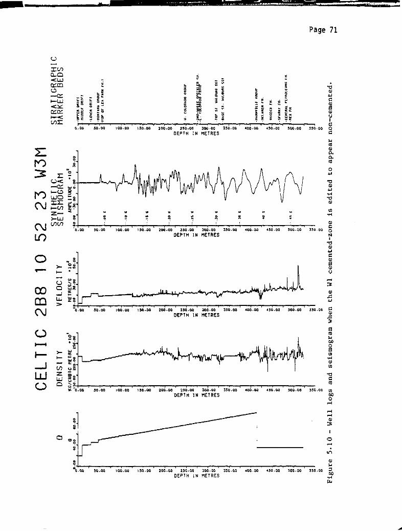
...
c>o
.,c>
o
fTI
" ...
.......
XO
_gz
3 ....
fTlg......;uo
fTloIn
o
o
00.00 40.00 10·00
g
...
o
g
CELTIC
DENSITY
KG/CUBIC METRE 0'0'
0'50.00 200·00 250.00
(:,I
' ,
I',
o
..
o
g
g;,o
...
o
Do
...
oo
.,o
o
fTI
" ...
.... ...
xC>;,
_..,
Z
�g......
:1:10
mc>UJ
g
g
"
...
<>
;,o
I288 10 23 W3M
g
g
'"
o
(,o
..
oo
g
uo
s
c..o
52
VELOCITYSYNTHETIC STRATIGRAPHIC
SEISMOGRAM MARKER BEDS
METRES/S 0102 AMPll TUDE 0' 02
�r0-60.00 -30.00 0.00 30.00
"fW'U�'n
g g -IfIOOlf 011'1'1
-lOilER OR,n
'" ..
., !' -IIOHU"_ GROUl'
0g IIor or lEA r_RK flf.1
o - .os S
g g 00
;, g '-.10 , .,
0 0
C; ;;; ;;;.. 0 0
g o -.ISC 0
0 0
...
g...
s0
0
(, 0 -
.20 .: ;,., 0 0
0 0 0
m '" ,.,
-U ... -UN " ...
....... .......
i �J ·u. 1'0lORAOO CROUPx� x?
_8 _8 -.Z5 C0
_0
z z z
1 =f�P;:MrAAlpgr���bFosu.
�g3.- 3'-
""8 ,.,g....
. ..... .....
:1:10 ::Vo ::Vo
,...0 ,.,0 -
.lO S �..
i--,orSI. IIUlIlJRG SSI.
en (IJ
... ... .... e.Sf. SI· lI�llllll\C 551 .
...
�...
.. 0
s ;, 0
0 ..
--- lS Ii
�!.. s
..
a
g
t.�."''' .....
-IfCURE" flf.
�i t"
� -
IIAG£C_ 'n .
0
o -SPARKY ,n.
-C[HfIlAl rHROlEU"'; flf.
H <.. 1-45 S
.>� �-RU flf.0
;,..
�J �J �J j J "
�
<> g ., Ul0 0
�
Figure 5.10 - Well logs and seismogram when the WI cemented-zone is edited to appear non-cemented. �
�
�

CELTIC
a DENSITY
0 KGICUBIC METRE -101
�O.OO40.00 10.00 01$0.00 100.00 150.00
0 gD
.. ..
0 0
., g0
a g0
g g
;.; �c 0
g g
., OJ
0
g0
., g0
0 0
f'l ,.,
"., " ..
..... '" ........
:r� :r�
_8 -gz Z
3<-1
�gfTIg...... .....
�g;00
f'lotn <n
�<-I
Co<> 0
g g
.. ..
s s
g g
.. ..
.. ..0 <>
g .,0
...
8
g
Co
�
g
288
VELOCITY
10
METRESIS _102
010.00 '0.00 50.00
.,"' , ' ,
o
eo
o
g
Figure 5.11 -
Seismogram with constant Q-value of 20.
L
g
g
i
g
...
g
g0
m
" ..
;;;_8z
3'"
f'lg......
�8tn
t0
g
..
s
g
..
...
0
g
...
g
g Ie:
52 23 W3MSYNTHETICSEISMOGRAM
AMPLI TUOE _102
O-to.oo -lO.OO 0.00 30.00
o ,.' , ,
i' I
o
� .-.05 S
.,o
g.-.10'
g
; 1-.15 S
o
g
� .-.20 S
o
go
1'1
"t: .-.2$ ,.....
0:r.
_8z
3'"1'1 g�-.JO S
;;g1'1
III
..,
...
�1-·JS S
g
gg 1-.40 ,
..
..
0
g�-'45'..
0
0
g
I
STRATIGRAPHICMARKER BEDS
·rwre« '"''
g -tIII1PLE I1ft,n
-LOWEn ORlff
...
� -IIIIIHAIIA GftOllP
g flO,. OF LEA 'ARK FI1.)
g
g
;,0
8
...
g(,D
0
m
" ...
; �_J.-U. COlORADO GROUl'
_8z
l:l�pcMrAUoArEfinb�DSH.
3'"
f'lg-t
•
:vg�t
lOP ". uALeURG SSI.
...-eAs"". UAlBURG ",.
...
D
s
..
8
g
f�"""'''�-
-IICLAREII fl1 •
..
� -WASECA fit.
g .
SPARK' Fit.
-G£"EftAL rUftOl[U,,& Fit·
� �-RO fit .
0
g
gJ "'0
QI
g to
1'1)
"-..J
N

00•00
u
o
...
o
o
o
o
o
o
o
..
o
o
o
'"
o
u-
go
....
-u..,
.......
:J:?o
_0
z
:iu",0....
0
�g(fJ
....
..
o
v
o
.
o
o
g
...
..
o
o
o
'"
o
o
o
o
::o
o
<>
a
o
40.00 80-00
CELTIC
DENSITY
KG/CUBIC METRE -'01
0150.00 ZOO-DO 250.00
oI
I ,
I't
o
...
?.,
.,
c;o
oo
..
.,
g
..,
.,o
go
....
-u..,
.......
:J:?o
_0
z
3 ....
.... 0
....0
�..... 8en
�o
s
...
to
o
g
...
o
o
o
o
<.
'"
0-
u
o
288 10
VELOCITY
METRES/S
olD-DO 30.00
_, 0250.00
o
o
..
o
oo
oo
g
..
o
.,o
..,
s
go
....
·U ..
..... ..
:J:?o
_0
z
3��O
�gen
u
..
o
g
.
g
g
to
o
g
1='"
o
o
o
o
f
'"
..
0-
Figure 5.12 -
Seismogram with constant Q-value of 50.
o
C>
L.
52 23 W3MSYNTHETICSEISMOGRAM
AMPll TUDE -, OZ_-60.00 -3D-DO 0·00 30.00
�II I I
::!:• ' ,
.,
��--05''"
o
o r-.'O'
o
o
o
lit... IS ,
o
g
g�-_20Sg
o
....
-U��-.Z5C.....0:x.
o
_0
z
3 ....
", g ... -.)O S......
�'"
",0en
Col
...
?1-- .)5 ,
g
.
.,
o
g �- 40 S
.
..
.,
0
: l4S'0
0
0
0
<.
'"
0
0
0
STRATIGRAPHICMARKER BEDS
o
g r�����EO=!�:'
o
o
o
o
�f'AR'" fn.
-lOIlER PRIH
...
?-j'nDH'AHA "flOIlI'
g IIOf' OF lEA "UK FI1.'
...
o
<>
o
�o
go
IT!
-U..,
-0'"
:x?v
_0
z
3'"
�g�.IT!gen
U. rOlORAOO f.ROIlI'
.
f�OrHrmoa"E�Bb�O�".
..
,Of' SI· �Al8I1RG 5S'.
....'-USE GI· IIAI.8URG s" .
'"
o
s
.
oo
g II1AHHHlH r.ROUP
IICLAREH fl1·
�J IIASfU fl1-
g
CorNUAl r[lROlFIJI1g (11_
� I IIU rn.o
g
...
'"
o
o
o
I
""C
£»
to
tD
.........
W

a
o
00.00 40.00 10.00
u
o
...
o
o
o
CA
�o
'"
;; ;;0 0
0 ;,0 0
;;; ;;;., 0
a (,0 .,
N N
0 0
., 0
g 0a
0 0
1'\ ,..
-UN -UN
...... .... '"
::r!' ;t;!,0 0
_0 _0
z :z
3'" 3'"",0 ,..0..... � .... �::00 ;00
",0 ,..0(/) lJJ
... ..
to '"
a 0
0 0
" 0
g.
0
0
0 0
0 0
.
�...
0 0
0 0
0 0
g0
0
CELTIC
DENSITY
KG/CUBIC METRE .'°1
olSO.OO 200.00 250.00
o
a
288 1 0
o
o
o
o
(A
o
o
o
CI
m
-UN
....'"
:r�o
_0
z
3'"
,..,0....
0
::00,..,e>UJ
....
to
o
o
<>
..
o
o
o
'"
...
o
o
o
VELOCITY
METRES/S .'°230.00 50.00
...
...
o
Figure 5.13 -
Seismogram with constant Q-value of 100.
<>
o
�-
SYNTHETICSEISMOGRAM
AMPLITUDE ·,o20-(>0.00 -30.00 0.00 30.00
r' , , , I I
52
"
o
� 1- .05 S
o
o
gt- .10 S
..o
�.--.15 C
o
o
� .-.20 S
o
(,o
o
",
'! � ,- .as G
::r!'
_gz
3'",... g .... - .30 S.... .
::00
('10(n
...
'"
!'1·-.JS'
s
.- .•0 S
..
'"
o
s 1_ •• s So
..
o
o
o
o
'"
...
o·
g
23 W3MSTRATIGRAPHICMARKER BEDS
o
g T�����/=!�:I
o
o
(,o
'HCLARO 'H .
·
LOIIER PRIH
'"
!'-J-HOHIAHA GROuP
g flor or LEA PARK rH.'
to
o
g
(;)
'"
-UN
.... to
::r0o
_0
z
�g.....
;00
,..0lJJ
- U. rOl OIUPO CoROUI'
:f�o;:lft'mD�pF.Ii�b$°�II.
· lOP �,. WAlBURG GH·
....eASE SI. IIALIIURG SH .
�
(,o
.
o
(>
g 1 -HAHHVlLLE r.ROUP
..
�1-WA&fr.Arn .
o . �PARK' rn.
· tEMERAL I'ElROlfUHS rll.
g I RfX rH·
g
I
-c
Q1
to
I'D
.......
.J::o
--- -- ... _.- -
• .._ ••.••••·' .. r .... , "".'.�.,��
Page 75
equal to 20, 50, and 100 are shown in Figures 5.11, 5.12, and 5.13. The
corresponding amplitude-spectra are in Figures 5.14, 5.15, and 5.16.
All of these tests were computed with an impulse source buried at 0.0 m;
therefore, they must be compared with the seismogram in Figure 5.17,
which was also constructed with an impulse source at 0.0 m but with the
standard Q function. The amplitude spectrum corresponding to this
seismogram in shown in Figure 5.18.
In comparing the seismograms of Figures 5.11 through 5.13, it is
immediately noticeable that the frequency content of the Mannville
sections is increased in the higher-Q seismograms. This observation is
verified by the amplitude spectra in Figures 5.14 through 5.16. With a
Q curve equal to 20, the general shape of the Mannville portion of the
seismogram of Figure 5.11 is similar to that of Figure 5.17, but the
high frequencies required for reflections from the McLaren coal-bed, and
the W6 and W3 oil-saturated sands are not present. With a Q curve equal
to 100� the general shape of the Mannville portion of the seismogram in
Figure 5.13 is also similar to that of Figure 5.17, but the
high-frequency content is now enhanced and the McLaren coal-bed, and the
W6 and W3 oil zone reflections are distinct and of large amplitude.
With a Q curve equal to 50, the Mannville portion of the seismogram in
Figure 5.12 is almost identical to that of Figure 5.17. The
corresponding amplitude spectra in Figures 5.15 and 5.18 are also
similar. The approximate average of the standard Q function is 50.
Therefore, the test with Q equal to 50 illustrates that, within
reasonable limits, it is the average value of the Q curve, and not its
shape, that is more important to the character of the Mannville portion
of the resulting seismogram.
The effect of a change in Q is more apparent in true-amplitude

Page 76
CELTIC 288 10 52 23 W3MCONSTANT 0=20.
SOURCE BURIED AT A DEPTH (M) = 0.0
TYPE OF WAVELET : IMPULSE
BUTTERWORTH ANTI-ALIAS FILTER INCLUDED IN SYNTHETIC TRACE
TIME GATE (IN S) FOR AMPLITUDE SPECTRUM = .dOS TO 0.493
TIME GATE CORRESPONDS TO:
TOP OF MANNVILLE GRP. (414.0 M) TO END OF INPUT LOGS (S23.2 M)
SAMPLE INTERVAL IN TIME DOMAIN (5)" .0010
SAMPLE INTERVAL IN FREOUENCY DOMAIN (HZ) " 7·812
NUMBER OF FREOUENCIES ANALYSED = 65.
HANNING SMOOTHING APPLIED TO SPECTRUM
PERCENT OF TRACE ELEMENTS TAPERED AT EACH END" 10.
AMPLITUDE SPECTRUM OF SYNTHETIC SEISMOGRAMo
o
o
o
Cl
�g::;0<
....
1:
a::
�go'"
o
:0-+.-00--'--50"".0-0--"-10-'0-.0-0....---15-.0-.0-0....---20-.0-.0-0-,---25'0-.0-0-,---30'0-.0-0""T-"-3S-'Or.0-0"'--40-'0',0-0-,--4'50'.O-O"-�-'OO. 00
FREOUENCY IN HERTZ
Figure 5.14 -
Amplitude spectrum from seismogram constructed with
constant Q equal to 20.
....

Page 77
CELTIC 288 10 52 23 W3MCONSTANT 0=50.
SOURCE BUR I ED A T A DEPTH (M) = 0.0
TYPE OF WAVELET : IMPULSE
BUTTERWORTH ANTI-ALIAS FILTER INCLUDED IN SYNTHETIC TRACE
TIME GATE (IN S) FOR AMPLITUDE SPECTRUM = .405 TO 0.493
TIME GATE CORRESPONDS TO:
TOP OF MANNVILLE GRP. (414.0 M) TO END OF INPUT LOGS (523.2 M)
SAMPLE INTERVAL IN TIME DOMAIN (S)" .0010
SAMPLE I NTERVAL IN FREOUENCY DOMA I N (HZ) = 7. B 12
NUMBER OF FREOUENCIES ANALYSED = 65.
HANNING SMOOTHING APPLIED TO SPECTRUM
PERCENT OF TRACE ELEMENTS TAPERED AT EACH END = 10.
AMPLITUDE SPECTRUM OF SYNTHETIC SEISMOGRAMo<>
o
o
o
<>
w�o
::::I....
-0-lo
�g<
o
WoNC')
::;0<1"1:a::
�goN
o
"
o+-�--��--��--�-'--�-'--'--'�'-��-r-'r--r�r-.--'��0.00 50.00 100·00 150.00 200.00 250.00 JOO·OO JSO.OO 400.00 450.00 SOO.OO
FREOUENCY IN HERTZ
Figure 5.15 -
Amplitude spectrum from seismogram constructed with
constant Q-equal to SO.

�� __ . __ .. __�__
...
-...w......... �_
-".-I .. ·��.�t .. � .....o:-# ....• •••�_ _._ ....__ .....
-
."
Page 78
CELTIC 288 1 0 52 23 W3MCONSTANT Q"'100.
SOURCE BUR I ED A T A DEPTH (M) = 0.0
TYPE OF WAVELET : 1 MPULSE
BUTTERWORTH ANTI-ALIAS FILTER INCLUDED IN SYNTHETIC TRACE
TIME GATE (IN S) FOR AMPLITUDE SPECTRUM = .405 TO 0.493
TIME GATE CORRESPONDS TO:
TOP OF MANNVILLE GRP. (414.0 M) TO END OF INPUT LOGS (S23.2 M)
SAMPLE INTERVAL IN TIME DOMAIN (S):: .0010
SAMPLE INTERVAL IN FREQUENCY DOMAIN (HZ) :: 7.812
NUMBER OF FREOUENCIES ANALYSED = 65.
HANNING SMOOTHING APPLIED TO SPECTRUM
PERCENT OF TRACE ELEMENTS TAPERED AT EACH END = 10.
AMPLITUDE SPECTRUM OF SYNTHETIC SEISMOGRAMo
o
o
o
o(']
w�o
�.....
-0-' (']
0...
1:�-e
o
�g:;0<.-1:
a::
�go
N
o
:+--T--��--��--��--��--'-�--'--'--'--'--'--'--II-.r-�0.00 50.00 100.00 150.00200.00250.00300.00 :lSO.OO �OO.OO �SO.OO 500.00
FREOUENCY IN HERTZ
Figure 5.16 -
Amplitude spectrum from seismogram constructed with
constant Q equal to 100.
....

I:)
,..,
-u ...
.... '"
L�o
_0
:z
3'",...0__,<>;0;',..,<>UJ
a
a
00.00 40.00 110.00
. I I' , ,
.,
o
to
o
'"
o
CELTIC
DENSITY
KG/CUBIC METRE 010'
0'50.00 200.00 250.00
I ' ' , ,
gi
..
o
g
o
o
..o
..
o
o
o
.,
g
go
,..
"'N.......
x�o
_0
%
3'",..0-to;00,..0(IJ
...
to
<>
g
..
so
a
..
..
o
(,o
g(,o
..
'"
t>
'"
o
288 1 a
go<>
'"
o
o
<>
'"
s
s
'"
to
o
e
o
..
o
'"
o
o
VELOCITY
METRES/S _102
0'0.00 30.00 50.00
I' , , ,
gi
:;
g
'"
'"
o
o
'"
<>
o
o
o
::::o
o
<>
g<>
<>
...
o
oD
'"
soC>
CJ
,..
." ...
.......
xC>o
_0
%
3'"
�?;00
,..,0en
g(,o
..
..
<>
o
<>
'"
...
o
o<>
Figure 5.17 -
Seismogram with standard Q-function.
L
52 23 W3MSYNTHETICSEISMOGRAM
AMPLITUDE _IOl
0-60.00 -30.00 0.00 30.00
(, II • • , , ,
<>
%
��-.OSS
g
g 1-- iO S
o
g
t.0- IS Ii
oo
g.-.lO S
gI:)
,..
!g.-.lSS:r.
_g
3'",.. g-l-.JO ,-to
;00
,..0(n
'"
...
�1--.3S S
g
g
g .- 40 S
...
0
0
o
�'-.�SS
..
0
0
0
<>
...
...
0
g
�GAS
STRATIGRAPHICMARKER BEDS
<>
8 r�����/:!�;r
<>o
u
<>
�n rN.
'LOIIER PRlrr
'"
? j.
!ION lAMA GROUP
g '"0P or LEA PAR� FN.'
'"
o
g
.,
sc,o
o
'"
-u.,
..... ...
:r�..
_o
z
3'"
�?;00
,..,0UJ
..u. rOlORAPO GROUP
:f�PrllrmD5PF.finb�0SN.
lOP �I. WAl8URG SSI.
....8Af'E s,· IIAl8Uft<, S�I .
..
o
C,o
gg I·NAH"�lllr. GROUP
.
NCLARFM rN .
..
� 1·I.I�Sf.c.. fri·
o �PAft�y rN •
.
f.UFRAl PEiROlrUNS nt.
I
-0
QI
CO
CO
.........
co

� � ����- --------
• ••�
•••• ,,,._ .. ., r.t'" <r'.!...:-. �.r.'
Page 80
CELTIC 288 1 0 52 23 W3MMINIMUM 0:20 AND MAXIMUM 0=100
SOURCE BURIED AT A DEPTH (M) = 0.0
TYPE OF WAVELET : iMPULSE
BUTTERWORTH ANTI-ALIAS FILTER INCLUDED IN SYNTHETIC TRACE
TIME GATE <IN S) FOR AMPLITUDE SPECTRUM = .405 TO 0.493
TIME GATE CORRESPONDS TO:
TOP OF MANNVILLE GRP. (414.0 M) TO END OF INPUT LOGS (523.2 M)
SAMPLE INTERVAL IN TIME DOMA.lN (5) = .0010
SAMPLE INTERVAL IN FREQUENCY DOMAIN (HZ) = 7.812
NUMBER OF FREOUENCIES ANALYSED = 65.
HANNING SMOOTHING APPLIED TO SPECTRUM
PERCENT OF TRACE ELEMENTS TAPERED AT EACH END = 10·
AMPLITUDE SPECTRUM OF SYNTHETIC SEISMOGRAM
100.00 lSO.OO 200.00 250.00 JOO.oO 350.00 400·00 450.00 "i00·00
FREaUENCY IN HERTZ
Figure 5.18 -
Amplitude spectrum from seismogram constructed with
the standard Q-function.

-
�----�
• •
•
•• & -
....- '_""�""·.f.!I'lIII':r...."..._••........
Page 81
plots. The same synthetic seismograms that were plotted with gain
control in Figures 5.11 through 5.13 are shown plotted without gain
control in Figures 5.19 through 5.21. In all three true-amplitude plots
the high-amplitude, direct-wave has been muted to increase the scaled
amplitude of the deeper reflections. Nevertheless, the amplitudes of
the reflections are quickly reduced, especially when a low Q value is
input. In Figure 5.19 (Q equal to 20), Mannville reflections are barely
visible. In Figure 5.20 (Q equal to 50), very low-amplitude
McLaren-coal and W6 and W3 oil-zone reflections are visible. In Figure
5.21 (Q equal to 100), the coal and oil-zone reflections are readily
visible. Therefore, if the Q function of the earth is similar to, or
less than, the standard Q-function chosen in section 4.5 (that is, with
an average value equal to or less than 50), then the oil-zone
reflections will be very difficult to identify on a true-amplitude plot
of real seismic-data. However, if the actual Q-function in the
subsurface has an average value that is higher than the standard
Q-function chosen for the present study, then the reflections of
economic importance should be visible on a true-amplitude
sei smi c- secti on.
The value of Q is critical in determining the frequency content of
the synthetic seismogram; if higher values of Q had been chosen for the
standard Q-function (section 4.5), the resulting synthetic seismograms
would have contained higher frequencies. A case could be made for using
higher Q values than those that were chosen, but these values were
considered to be realistic based on the available literature (see Table
4.5). Until in-situ attenuation studies are undertaken in the study
area, the Q values can only be estimated.

...
a
.,
"
.,
o
m
" ...
--.'"
:r?o
_0
z:
3«
�g:<Ie,mOVl
o
o
�.OO W.OO ".00
<>
o
..
g
o
o
g(,.,
o
m
." ...
.... '"
:x:�.,
_0
z
3 ....
mO....
0
:<10moU1
CELTIC
DENSITY
KG/CUBIC METRE ·'010150.00 200.00 2S0.00
a I. I
",
o
I288 23
'"
.,
s>
o
'"
o
oo
o
o
.,
o
..
o
.,
.,
..
so
o
..
...
o
.,
.,
go
.,
10 52 W3M
.,
.,
.,
o
...
.,
<>
o
...
'"
c-
o
o
..
'"
o
g
VELOCITYSYNTHETIC STRATIGRAPHICSEISMOGRAM MARKER BEDS
METRES/S .102 AMPlI TUDE .101
010.00I
JO.OO 50.00 .,-§o.oo -20.00 20.00 &0.00
? ·urru ORIFf
idLl, I I I
g_1I
'=:1I I , I
"1".." �'"
LOWER PRlr.
'"
:1''' 1to
.,? MO"IAHA GROUP
(,g Clor or L(A PAftK Fn.'.,
(; (;.,-.10 S
., 0 c-
o ., Cl0 ., .,
;;; ;;;- .15 S ;;;
., ., 0
0 0 Cl0 0 .,
...
�-
.20 $IV
0 00 0 0
0 (, <>
0 0 0
0 0 0
m m m
." ... "'N·-.25 S
" ...
...... ......
:;�.J. U. COLORADO r.Rour:I:� :r?
0 0 <>
_0 _0 ..... 0
z z z
1 :l�OiHLI&UD5r���bFDStf
3'" ;:S ... ;:S ..
mg fTlo- .JO S
mO--f • -f� --.0;00 ;00 :<10
mO 1'10:;:.,
i·'or sr . WALIIUIIG �q.
U1 U1
... ... ... 8�Sf Sf WALBURr. <q .
.. '" ..
0 0- .35 S
0
., ., .,
0 0 t>
g.. ..
.,
g0
0 o � ·.0 � ·
r"'"'',,-0 0
tfCLARr.H fit .
.. .. ..
.. '"
g .
WAsrCA rH.0 0-
0 <> 0
., .,·.4S S
o ··C;PA"'''' fH .
i � :ito
(-[MfRAl rrrROLfUHS rH·
gRU 'n.
0
o
J �J J �J �J'"0
CI
., 0 ., '-0<> 0 0
I'D
Figure 5.19 -
Seismogram with constant Q value of 20; plotted with gain control. ex>
N
�

CELTIC 288 1 a 52 23 W3M
0 DENSITY VELOCITYSYNTHETIC STRATIGRAPHICSEISMOGRAM MARKER BEDS
0 KG/CUB I C METRE -'0' tlETRES/S _ 102 AtlPl J TUDE -10'
00.00 40.00 '0.00 0'50.00 200.00 250.00
:0 TOO' '�, ";" , ? -urr[� DRlrl
I' , '----L-J
s I' ,
;::JI I ,
s I g
I"""" .,,"
-lOW[� ORIFI
'" '" ;:_ .n...
0 0? -ItONIANA GROUP
" <>
g HOP or LU "R� fH. t0 '"
(; (; ;; o ,,·'0 S Iip 0 '"
?0
0 0 ., 0 ;,0 0 '" ., '"
;;; ;;; ;;; ;;; --.IS' ;;;0 0 0 ., '"
e> 0 0 0 0
0 0 0 0 0
'" '" ... '" - .20 �'"
0 e» ., ., 0
0 '" '" '" .,
p g .. g "'" '" o
CJ CJ 1::1 CJ CJ
III ".. ".. III tTl
" N ." ... ." .. ." ...- -25 ,
,,'"
-<Of � ... .... '" -<'"
;;. �_J -U. cOLORADO CROUP:r? :r? z? :r?
t>
_&0 0 0
_0 _0 _0 _0
:z Z z :z :z
1 :l�O;:HrAUo5PF,m�o<N.
3 ...
3� 3'" 3'" 3 ...
,..,0 "..0 ,..,0 ..... 0
-<?"'0
.... ? -<0-- .JO , -fo--t •
,",0 ,",0 ;00 ;00 ;00
..... 0 fTlo (TIo ,..,0�
0
I_lor sr . IIALBURG S<I-
(I) (/) In In
u ... ... ... u
-
BASE SI - IIHIIURG <U
'" '" ... '" '"
0 0 <> '"-. J5 S
0
0 ;,g
0 ;,0 0 0 '"
.. . . . .
o 0 0 0 0
0 0 '" 0 0
" '" <> u -
."0 S g
1m"..", ,-o <> '" '"
'!CLAnEH fH·
..
t;,.
t:.
'" '"
g UASf.r.a rn.0 <> o 0
<> o <>
g0
'" " 04S S
o (PARIH Fit.
�1 I H -s.. H � HOf
<EHERAl pnROLrUtt< fH.
'" Rn fit.0
'"
0
...
(A
t>
P
<>
<.
(A
0_
oo
'"
(A
o
.o
<>
'"
l:
g
'"
:;
<>
.o
Figure 5.20 -
Seismogram with constant Q value of SO; plotted with gain control.
�
I
""0
AI
c.Q
CD
00
W
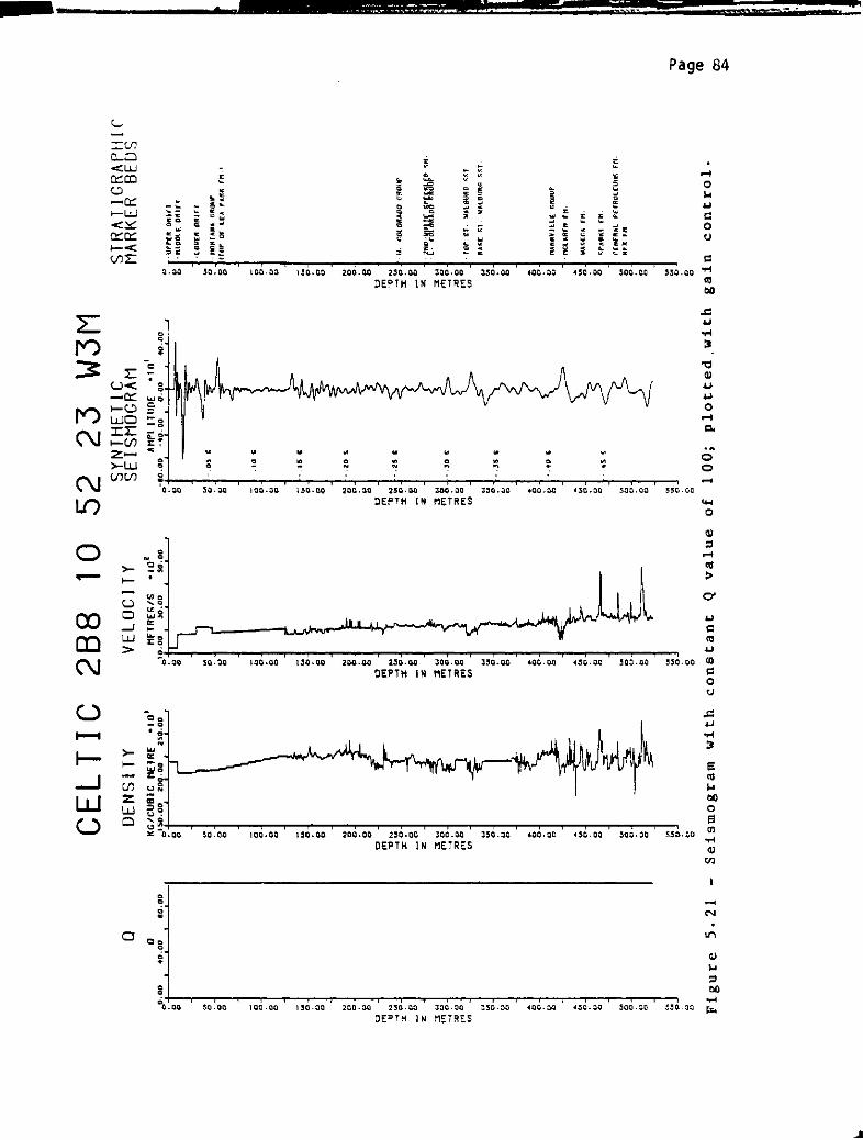
a
a
00.00 40.00 10.00
.,
o
'"
o
<>
o
o
fTI
"N
.......
x!'o
_0
z
3 ...
",0....
0
;:00",0I/)
CELTIC
DENSITY
KG/CUBIC MEJRE 0'0"
0"50.00 200.00 250.00
oI
« ,
if,
<>
...
o
o
o
288 1 0 52 23 W3M
VELOCITYSYNTHETIC STRATIGRAPHICSEISMOGRAM MARKER BEDS
METRES/S 0' 02 AMPl I JUPE 010"
0"0.00 lO.OO 50.00 0-80.00 -40.00 0·00 40.00
"l��'�'"
g ILt"I I I ,
(,g -nIOOlE ORin0
-lOUER ORin
'"
� - .OS ,...
0?
-
ItOH , AHA r.Rour
c> 0
g lIor or lEA PARK rlt -,0 0
(; o -.10" (;0 0 0
;, 0 o
., 0 <>
;;; ;;; -.15" ;;;0 0 0
0 0 0
., 0 <>
..
�- .20 S ...
0 .,0 0 0
;, u 0
., 0 .,
0 0 0
fTI ..... .....
"N -U ...- .25 C
-UN
...... ..... '" .... :; J U. COlORADO "�OlJPx? x? x.
_g -g0
_0
z z z
1 l"O;�L'AnoSP���bFP<H_
3" 3�3 ...
fTlo .....0 -- -'0 G
",0.... ? ..... .... ?
�g;:00 ;:00
",0�
0
i-for.,. UAlOIJRG <<I-
I/) I/)
,. .... ...
-
0'.[ �I. WAlDURr. <<1-
'" '" '"
0 .,- .'5 C
D
0 0 g., D
... ... ...
0 0 0
D 0 0
0 o -.40" g
I�...'''''.-D .,
nclAft£" fit.
fi r-:;.
...
0 g "��Er.A rn_
0 0
r=0
45 So �rARK1 Fn
([HUAl PElROl[UI1< rlt
i'"
� REM Frt0
0 .,
0 0
0 0
..
....
o
o
o
....
....
o
g
�D-
C>
<>
o
o
<>
<>
..
o
u
o
1:1
'"
-u eo
--<'"
:r?o
_0
z
3u
''10....
0
;.v�",0VI
..
'"
o
<>
o
...
o
o
g
..
..
o
g
'"
oo
o
o
o
o
.,
o
..
.,
o
o
...
o
.,
g
...
.,
o
<>
o
..
o
o
.,
...
o
o
.,
.,
Figure 5.21 -
Seismogram with constant Q value of 100; plotted.with gain control.
�
I
'"Q
QI
to
(1)
0)
...

,_"'-- -----�.
'" •••••,••• �.,'
•• ' ..
t'.{.., .....I'1"!".,........""''''fl�.
Page 85
5.3.4 Depth of Source Burial
Tests were made with synthetic seismograms that were constructed as
if the source were buried at depths of 0.0 m, 9.8 m, 29.9 m, and 46.7 m.
These depths correspond to the tops of the surfi ci al 1 ayers, �,hi ch are
in the cased portion of the wells; the time to depth conversion in
CELGRF was set up to handle only these depths. Using input parameters
of an impulse source and the standard Q-function, the four source-burial
cases are shown in Figures 5.22 through 5.25. In each of these plots
the direct wave has been muted if the source is located below the
surface. The corresponding amplitude spectra are presented in Figures
5.26 through 5.29
As one would expect, when the source is buried more deeply, there
is less influence from the highly absorptive surface-layers, and the
frequency content of the Mannville section of the seismogram is
increased. The amplitude spectra of Figures 5.26 through 5.29
illustrate this tendency.
The overall shape of the lower part of the seismogram varies in
Figures 5.22 through 5.25. This is in part due to the change in
frequency content that was discussed above, but is mainly the result of
interference from a type of multiple reflection called a ghost. Ghost
energy travels upward from the shot and is then reflected downward,
jOining the downward-travelling wave-train and changing its shape
(Sheriff, 1973). Since the synthetic seismograms were constructed using
a reflection coefficient of the surface (from below) equal to 1.0, the
ghost reflections will be of high amplitude.
The response of the geologic zones studied in section 5.3.2 varies
among the four source-burial cases. The character of some reflections
is significantly altered by different depths of source burial. For

gg
o
m
" ....
_,,,,
:x:?a
�O
:z
3'-'1'10_,
0-
::vomo
en
o
o
00.00 iO.OO 80.00
. I II I I
g
o
o
C,o
CELTIC
DENSITY
KG/CUBIC METRE ·'0'
O'SO.OO iOO.OO lSO.OO
II , , ,
gI
...
o
o
o
go
o
...
o
o
o
o
'"
" ....
_, ..
:x:?o
�O
Z
�g....
::Va
",0en
..
s
oo
...
'"
o
g
go
o
'"
..
.o
o
o
288 10 52 23 W3MSYNTHETICSEISMOGRAM
AMPlITUOE • 10l
0-60.00 -30.00 0·00 30.00
o I' I I
I , I
o
� I· .OS S
g
g1'- 10 S
a
o
CA·-ISSo
g
l- - zO S
o
'"
!� i-·iS S
x?a
�(J
Z
3'"
� g .. ·.JO ,
::VO",0(It
...
..
?1--_JS S
s
..
00
<, I- .40 S
0
...
...
0
(;,o
�4S S
...
0
0
<>
0
...
...
0
<>
0
Figure 5.22 -
Seismogram with impulse source buried at 0.0 m.
Co
o
a
a
...
0-'
a
o
:.:o
.,
.,
go
c»
..
o·
o
...
...
...
o
o
o
VELOCITY
NETRES/S ·'Ol
��T·O_0-L_3_0�.0_0�L-s_0�.0_0s
...
o
g
go
.,
..
o
<>
o
'"
g
go
'"-0'"......
x?o
�o
Z
3'"",0....
0
::vo",0(It
...
..
o
oo
g(;,o
'"
<>
g
�<>
g
STRATIGRAPHICMARKER BEDS
? -UPPER pnlFl
s l-"IDOlF pnlff
sa
o
-
"clIRn fit-
-lO�£R PRIFl
(A
?
iItOH""" GROur
g HOP Of" LEA r,uttc rH.'
...
o
C,<>
g(;,o
o
'"
" ...
... ..
:r:?<>
�<>
z
3'"",0_.0::VO1'10(It
-U. rOlORAPO CROUP
-,l�orMrmD5PF.fi�b�P�It.
lor SI, WALBURG ,SI
....-BIS£ SI_ WalBURG SGI .
IA
<>
s
..
g
s I I1IHH�Ill[ CROUP
..
� 1"""srCA FH .
a c;rARKt' f"n •
r.(HfRAl PElROl[Un.< rlt.
� I �r. rn .
o
o
v
, .
'"
o·
<>
<>
I
""0
QI
CO
(1)
(X)
0'\

IU
o
o
go
,.,
,,'"
.....'"
:r?o
_0
"Z
3 ....
",0-to::o�"",<>en
o
a
00.00 40.00 10.00
. I I' , ,
s
'"
o
g
CELTIC
DENSITY
KG/CUBIC METRE _10'
0150.00 200.00 250.00
I« « « I
gi
...
o
g
g
g
...
o
g
'"
s"o
o
",
-P ....
.......
:ro"
_0
z
3 ....
�?;;00
",0I1J
....
...
o
g
g
g
..
'"
o
o
o
'"
...
.,
.,
o
288
VELOCITY
10
METRES/S ., 02
0'0.00 lO.OO 50.00
t' , « f
gi
...
o
g
52 23 W3M
.,
o
s
'"
o
"<>
..
o
o
o
o
'"
o
o
.,
'"
.,
.,
o
.,
'"
'"
.,
o
.,
g
g
SYNTHETICSEISMOGRAM
AMPll TUDE _ 102
0-60.00 -lO.OO 0.00 30.00
oI
« « «
I« «
o
z:
...
o
"o
goo
o
",
-p",
..... '"
XOo
_0
z
3 ....
",g_, .
;::gU>
....
'"
o
g
..
s"o
'"
g
o
<>
...
'"
o
<>
o
�O"i-.OS 5
o
it--.IO 5
.,0
�""-.15 S
00
gg
o
",
" ...
_,..
x!'
-g
�g_, .
:;00
",0I1J
�- .JS ,
�o
g1-.40 C
..
'"
o
<>
o
'"
o
o
.,
o
Figure 5.23 -
Seismogram with impulse source buried at 9.8 m.
L
-.20 C
- ·25 ,
- .30 S
-. <5 5
I
STRATIGRAPHICMARKER BEDS
"rwn•"'"
g nlDDLE DAIH
-lOIlEIl Dlllf!
'"
� -IID"U"� GROUP
g II0r Of lEA rA"1t ,n.'
<;0
(,0
;;;0
g
gg
0
",,,'"
;. �_. -u. COlORADO ClftOUr
0
_0
:z
1 �f�Pclll'AUD�r�finbJD&It·
3 ....
",0.... ?:;00
�0
i"lor". IIALBURe 'SI.
...-SASE SI IIALBURG 5SI .
'"
0
..0
..
0
0
"1�...n" ,,-
·rteLARU fft .
..
� -IIAS[eA rn.
0
a ,,..IIKI 'n.
-r.EIf£AAl rrrROlfUn, rn.
� I,,"EW ,n·0
.,
0
j"1:J
III
c.Q
t1)
co'-I

CELTIC
0 DENSITY
ltG/CUBIC "ETRE -.01
0°·00 40.00 eo.oo 01$0.00 200.00 lISO.OO
" ga
.. ..
a a
0 ..a CO
0; ga
g g
;; ;;0 C>
0 g0
OJ ...
a
ea
0 gCO
0 0
r>1 r>1
"01 "OJ...... .... ...
:r� :r:�
_8 _8z z:
3� �gPIa....
. .....
;00
�g.....0
(II en
..
t:..
0 ..
g g
g gg g
... ...
to ...
a a
g "a
..
0
0
g
...
..
a
g
..
�
g
288 10 52 23 W3M
VELOCITY
MEJRES/S -. 0'0'0.00 30.00 SO.OO
I' , , ,
g•
t
g
SYNTHETICSEISMOGRAM
AMPll TUOE - • O'
!"-ro,oo• -".00 I o'r . 30jOOg
..
C>
� fOSS
g
g t- .• 0 S
;;C>
g .-.15 C
...
0
0
g haD C
0
r>1
" ...
--'"
:r:�
_8.-.15 C
z:
�g.....
"'gc: .-.lOC
�C>
g
+.15 C
g.
g
1--.40 C
...
..
a
g
..
�.-.05 S
..
0
..
..
e>
g
Figure 5.24 -
Seismogram with impulse source buried at 29.9 m.
L
ig
i
g
ig
o
r>1
:!t::1:0
_8z
:sg�o:G'r>1gen
t:o
g
gg
...
..
o
g
gg
..
..
o
g
I
STRAtiGRAPHICMARK R BEDS
ernM'"
g -III DOlE Olliff
-lOIlEIl DIll"
...
� -11II"""A 'JlUII!'
g nDr OF lU 'All_ ,,,.,
g
g
;;C>
g
...
g
g0
r>1
" ..
; �.! -u. tOlOIl_oo 511oUl'
_8z
1:i�;;IIt'&np6I"U&��OSII.
:s ..
",0_,e>
eg
i-fOP Sf. IIAlIIIIIIIl 551.
Col-IIASE Sf. IIAllIUIIG 5SI.
...
0
g
g
gr-«"'--ltClAlI(" ,n .
_.
t -IIASECA rll.
0o .
-S'AII'" rn.
-CEMEIlAl 'EIIIOlEUItS '".
� 1-11[1( r" .
0
g
�j -0
Q).,
cao
CD
00
00

.,
o0-
gI:>
",
-U'"
........
I?.o
�O
z
3 ...
m(>...
0
:;1Jo",.,
(J)
o
a
�.oo W.OO ".00
oo
'"
o
(>
o
CELTIC
DENSITY
KG/CUBIC METRE .10'
0,50-00 too.OO 150.00
.,o
...
o
.,
.,
o
o
o
o
....
o
g
OJ
o
!"o
o
o
",
-u ..
.......
XO
�g:z:
3'"
",0.....
0
:;1Jo",0(J)
u
..
.,
g
...
s
g
...
..
.,
o
.,
'"
o.,
g
'"
...
o
.,
.,
288 10 52 23 W3M
o
o
.,
.,
VELOCITY
METRES/S _'020'0.00 30.00 50.00
. Ii' , , •
g
...
o
g
g
g
u
o
g
..
g
go
",
-u ...
.... ..
I!".,
�o
:z:
3'"",0....
0
�gen
t:.,
g
...
'"
o
o
o
'"
o
.,
"o
...
to
-c
o
..
SYNTHETICSEISMOGRAM
AMPLI TUDE - 102
!,,-�O.OO-30.00 0·00 30.00
.,
__L_�-L�__ L-�
o
...
0
.,0
{--OSs
g"o
{-_ID6
u
0
g �-.IS ,
OJ
g0
OO.-.ZDS",
-U ...
...u
:r!"
_g:z: _J.-.as c
3'"",0.... !"
�g(J)
1-.30 S
u
..
0
g
t- -JS S..
00
0
.,
.. 1- -40 Sto
0
g
...
o
!"� - 45 S
o
.,
'"
'"
<>
.,
.,
Figure 5.25 -
Seismogram with impulse source buried at 46.7 m.
L
'"
o
s
...
'"
o
o
(>
...
.,<>
u
<>
..
'"
.,
g
I
STRATIGRAPHICMARKER BEDS
T""�'"g -n'OOlE ORIFI
-lOUEtI ORin
...
? --IIO"'A"A r.Rour
g nOP or LEA PAil" fll. I
(;o
g
;;;0
.,
0
...
0
.,
s0
f11
-UN
;_ ? -1-U. COlORAllO GROUP
�gz
I: fN"i'lfrmo5P�finb�O�H-
3u",.,
-t �.
:og�
i-lor&r. VAl BURG 5S!-
...-"UE sr , IIAUUAG S51-
...
0
(,0
..
0.,
;,
1m....." 'MW
IIClARE" rn
� v"srCA Fit
g -
sr."", rn.
r.[NERAL p[{ROHUm; fn.
� I IIU rn.
0
.,
.,
'"
� , "
<>III
., c.o
(D
00
ID

� _w ���_ __
." .. ,'. \" ....... ,�.�......
Page 90
CELTIC 288 1 0 52 23 W3MMINIMUM Q=20 AND MAXIMUM Q=100
SOURCE BURIED AT A DEPTH (M) = 0.0
TYPE OF WAVELET : iMPULSE
BUTTERWORTH ANTI-ALIAS FILTER INCLUDED IN SYNTHETIC TRACE
TIME GATE (IN S) FOR AMPLITUDE SPECTRUM = .405 TO 0.493
TIME GATE CORRESPONDS TO:
TOP OF MANNVILLE GRP. (414.0 M) TO END OF INPUT LOGS (523.2 M)
SAMPLE INTERVAL IN TIME DOMA.IN (5) = .0010
SAMPLE INTERVAL IN FREQUENCY DOMAIN (HZ) = 7.812
NUMBER OF FREOUENCIES ANALYSED = 65.
�ANNING SMOOTHING APPLIED TO SPECTRUM
PERCENT OF TRACE ELEMENTS TAPERED AT EACH END = 10.
AMPLITUDE SPECTRUM OF SYNTHETIC SEISMOGRAMo
'"
o
o
o
WoNo
:;0<"or1:
a:
�go
N
100.00 iSO.OO 200.00 250.00 JOO.OO JSO.OO 400·;)0 450.00 SOO.OO
FREQUENCY IN HERTZ
Figure 5.26 -
Amplitude spectrum from seismogram constructed with
impulse source buried at 0.0 m.

_.-...:......
_--_....-." ••• f' ••
,••• , ••• ..,'='.�
7 ,!: !
Page 91
CELTIC 288 1 0 52 23 W3MMINIMUM 0=20 AND MAXIMUM 0�100.
SOURCE BUR I ED AT A DEPTH (M) = 9.8
TYPE OF WAVELET: IMPULSE
BUTTERWORTH ANTI-ALIAS FILTER INCLUDED IN SYNTHETIC iRACE
TIME GATE (IN S) FOR AMPLITUDE SPECTRUM· .405 TO 0.493
TIME GATE CORRESPONDS TO:
TOP OF MANNVILLE GRP. (414.0 M) TO END OF INPUT LOGS (S23.2 M)
SAMPLE INTERVAL IN TIME DOMAIN (S) = .0010
SAMPLE INTERVAL IN FREOUENCY DOMAIN (HZ) = 7.812
NUMBER OF FREOUENCIES ANALYSED = 65.
HANNING SMOOTHING APPLIED TO SPECTRUM
PERCENT OF TRACE ELEMENTS TAPERED AT EACH END = 10.
AMPLITUDE SPECTRUM OF SYNTHETIC SEISMOGRAMoo
o
o
o
o
w:io
::::I
,_
-0...Jo
a...
l:�-e
o
WoNO
:;0<
....
1:
0::
�go
'"
o
:+--'--�-'--'--'--'--'--'--.--'--.--��r--r-'r--r--r--r--r-�0.00 50.00 100.00 150.00 200.00 250.00 300·00 JSO.OO 400.00 4!'i0.OO SOO.OO
FREOUENCY IN HERTZ
Figure 5.27 -
Amplitude spectrum from seismogram constructed with
impulse source buried at 9.8 m·

....Il-�,.w�__� ..__..III1I!I!II!b!t!!!!!!==!!!!!!!'::���:==:::::?l:;�::!:::::::S70��.��==�::'�;:�:
Page 92
CELTIC 288 1 0 52 23 W3MMINIMUM 0=20 AND MAXIMUM Q=100
SOURCE BUR I ED AT A DEPTH (M) = 29.9
TYPE OF WAVELET : IMPULSE
BUTTERWORTH ANTI-ALIAS FILTER INCLUDED IN SYNTHETIC TRACE
TIME GATE (IN S) FOR AMPLITUDE SPECTRUM = .405 TO 0.493
TIME GATE CORRESPONDS TO:
TOP OF MANNVILLE GRP. (414.0 M) TO END OF INPUT LOGS (523.2 M)
SAMPLE INTERVAL IN TIME DOMAIN (S) = .0010
SAMPLE INTERVAL IN FREQUENCY DOMAIN (HZ) =: 7.812
NUMBER OF FREOUENCIES ANALYSED =: 65.
HANNING SMOOTHING APPLIED TO SPECTRUM
PERCENT OF TRACE ELEMENTS TAPERED AT EACH END = 10.
AMPLITUDE SPECTRUM OF SYNTHETIC SEISMOGRAMo
o
o
o
o
LLlONO
:;0<
....
1:
It:
�go
'"
100.00 150.00 ZOO·OO 250·00 JOO·OO J50.00 400·00 450·00 500·00
FREOUENCY IN HERTZ
Figure 5.28 -
Amplitude spectrum from seismogram constructed with
source buried at 29.9 m.

----- _-
• • • •• ,. , '",
.• � •••.. "'Pf'
7¥ 2m, ?
....a-_$C�:._ .......�r
CELTIC 288 1 0 52 23 W3MMINIMUM a�20 AND MAXIMUM 0=100.
SOURCE BUR I ED AT A DEPTH (M) = 46.7
TYPE OF WAVELET: IMPULSE
BUTTERWORTH ANTI-ALIAS FILTER INCLUDED IN SYNTHETIC TRACE
TIME GATE (IN S) FOR AMPLITUDE SPECTRUM = .405 TO 0.493
TIME GATE CORRESPONDS TO:
TOP OF MANNVILLE GRP. (414.0 M) TO END OF INPUT LOGS (523.2 M)
SAMPLE INTERVAL IN TIME DOMAIN (5) = .0010
SAMPLE INTERVAL IN FREQUENCY DOMAIN (HZ) = 7.812
NUMBER OF FREOUENCIES ANALYSED = 65.
HANNING SMOOTHING APPLIED TO SPECTRUM
PERCENT OF TRACE ELEMENTS TAPERED AT EACH END = 10.
AMPLITUDE SPECTRUM OF SYNTHETIC SEISMOGRAMo
o
o
c
c
c
o+-�--��--��--��--'-�--,--,--,--,--�-.--,--,--.--,r-I0.00 50·00 100.00 150.00 200.00 250.00 300.00 350.00 400.00 450.00 soc.oo
FREOUENCY IN HERTZ
Figure 5.29 -
Amplitude spectrum from seismogram constructed with
impulse source buried at 46.7 m.
m:m:r=-- 7
Page 93

I
""'0
Q.I
c.o
(1)
\.0
01
.
Wo
Cl
::::>
._
WAVELET SHAPE
o
CJ;)
01 I , I I I I I I I , I I I I I
o
00
I
0.00 0.08 O.i6 0.24
T I ME IN
Figure 5.30 -
Velocity-type Ricker-wavelet with a peak frequency of 80 hz.
�

.... m��� __......... , ........
,.........
-._�
7
4 ="t•
Page 94
example, the reflection from the McLaren formation coal-bed in Figure
5.22 (0.0 m burial) is similar to that of Figure 5.24 (29.9 m burial),
but in Figure 5.23 (9.8 m burial) this reflection is not visible, and in
Figure 5.25 (46.7 m burial) the single peak has split into a doublet.
The W6 and W3 oil-zone peaks are distinct in all four seismograms, but
they are of highest amplitude in Figure 5.25 (46.7 m burial). As was
discussed in section 5.3.2, the small trough that was expected in
response to the WI cemented zone did not appear when this zone was
modelled. This non-appearance was attributed to interference effects.
The large trough that occurs in Figure 5.24, at the time that the small
W1 trough was expected, changes in character among the four source
burial cases. In fact, if the modelling of the W1 cemented zone were
repeated at a source burial different from 29.9 m, the expected W1
response may be visible.
A source buri al of 29.9 m was chosen to be the "best" for the
present study. Although the burial at 46.7 m returned the
highest-frequency reflections from the Mannville beds and the specific
reflections of economic interest were the most distinct at this depth, a
source burial of 46.7 is too expensive for routine seismic-surveys. It
is important to note that, even if a surface source had been used,
Figure 5.22 indicates that it is theoretically possible to record the
oil-zone reflections. For very detailed work, however, it may be
necessary to use a source burial deeper than 29.9 m.
5.3.5 Input Source
Test synthetic-seismograms were constructed using velocity-type
Ricker-wavelet sources of peak frequencies from 20 to 220 hz. A Ricker
wavelet of this type is shown in Figure 5.30. In Figure 5.31, the

7
d..... � ..... ,,_ ......_ .."'-.
=.... -�-�------------ 'T ;;;1' :o:=�
...
pe=mnc"!'t �?
Page 96
PHASE SPECTRUM OF INPUT WAVELEToo
o
�
W
(/)0<0
::1:'
o..gI
o
o
oN
o
o
o
00
'O;.�00�-;'SO�.:OO��1:00�.:OO��1�sTo�,o�O��20�O�.0�0,L�2�50:.-00-r-J-OOI.-DO�-J-S�0-.D-O'--40�0-.0-0-r-4-S0;.�OO����oo.ooFREQUENCY IN HERTZ
AMPLITUDE SPECTRUM OF WAVELETo
o
o
o
o
WCl
00:;''''.....
....J
0..0
EO
<0...
Q
Q
<:I'"
50.00 100.00 150.00 200.00 250.,:)0 JOO.OO 350.00 �OO.OO 450.00 SOO.OO
FREQUENCY IN HERTZ
Figure 5.31 - Phase and amplitude spectra of the Ricker wavelet in
Figure 5. 3 o.

_.-..,...".------ . ::
Page 97
amplitude and phase spectra of this wavelet are shown. This particular
wavelet has a peak frequency of 80 hz and a linear phase-response over
the band-pass. A linear-phase filter shifts phase proportional to
frequency, thus introducing a constant delay without change of
waveshape; the phase spectrum is linear over the band-pass and the
intercept must be a multiple of 2Ti(Sheriff, 1973). These
characteristics are seen in the phase spectrum of Figure 5.31. The
constant delay introduced by using the linear-phase wavelet may be
calculated from the slope of the phase spectrum (Titchkosky, 1968, p.
28-34, p. 37). With the 80 hz wavelet of Figures 5.30 and 5.31, the
delay was calculated to be 10.8 ms. At lower peak-frequencies, the
slope of the phase spectrum becomes steeper and the calculated delay
will be larger.
When the peak frequency of the Ricker-wavelet source is increased,
the high-frequency content of the resulting synthetic-seismogram
increases and the delay decreases. Seismograms that were constructed
using the standard Q-function and a Ricker-wavelet source buried at 29.9
m and of peak frequencies of 60, 80, 100, 140, 180, and 220 hz are shown
in Figures 5.32 through 5.37. The corresponding amplitude spectra are
in Figures 5.38 through 5.43. The trend of increased high-frequency
content with a higher-frequency source can be noted in the seismograms
and the amplitude spectra.
The anti-alias filtered, impulse-response seismogram (Figure 5.7)
is very similar, in the Mannville section, to the seismogram that was
constructed 'trith the 80 hz Ricker-wavelet source (Figure 5.33). Using
an 80 hz Ricker-wavelet source corresponds to filtering the impulse
response seismogram with a band-limited, 80 hz peak-frequency filter of
linear phase. Slight differences in the general shape of the Mannville

'"
o
o
(,I:>
o
,..,
-0'"__.'"
:r?o
�I:>
Z
3",..,0.....
0
::00,..,0U:I
o
o
�.OO W.OO �.oo
g
o
o
(,o
'"
goo
o
1'1
-0 ..
......
:roo
_0
z
3"1'10...
0
,",01'10'"
CELTIC
DENSITY
KGICUBIC METRE .10'
0150.00 200.00 250.00
,' . . ,
g,
288
VELOCITY
10
METRESIS .1020'0.00 30.00 50.00
I ' , , ,
g,
'"
C>
g
52 23 W3MSYNTHETICSEISMOGRAM
AMPLITUDE _102
0-60.00 -30.00 0.00 30.00
g
STRATIGRAPHICMARKER BEDS
? -UrPER DRIF!
g l-ItIDOlE GRiFf
s
g
-�'�R�' rn·
...
o
o
o
'"
I:>
o
'"
....
'"
'"
o
'"
..
o
'"
g
'"
o
g
goo
...
'"
..o
g
g
.
...
'"
oo
g
g
'"
C>
..o
gg
o
,..,
-0 ...
__. ...
:x0
_8z
'"
o
g J-.O$ S
g
g.-.Ios
;;.0
0.-.1$ C'"
.-.20 S
0
1'1• -0 ...
..... ",
:r?
_g .-.l$ C
z
3'"1'10...
0
,",0
�O�-.JOC...
'"
0
00
i-·JSS
..
0
0
00
{-.40 ,
...
'"
I:>
0
I:>
:; I .
- 4S S0
<>
I:>
...
'"
I:>
g
-LOVER OR'ff
..
? J --IIOHIA�A GAOur
g I flDr Dr lEA PARK fit. I
'"
o
oI:>
gUI:>
o
1'1
-0 ...
.....'"
:r0I:>
_0
Z
-U. COLORADO GROUP
=f�OiMl.'AU08PF.�nbFOSII.
..
...
o
'"
o
'"
g
o'"
�g;;g,..,en
�o
g
'"
I:>I:>
I:>
I:>
3'"1'10...
0
::001'10'"
·IOf 51. WALBURG 551.
....-I�SE 51. UAlIIUIIC SSI .
I;
g
...
I:>
I:>
g l-nAM"VlllECRDUr
--IICUREN Fit .
...
I; J IIASEr.A Fit.
g
'" 1-c[�ElIAlr£lROl[UltS fit·
g-RU Fit.
g
Figure 5.32 -
Seismogram constructed using a Ricker-wavelet source with peak frequency of 60 hz.
L
I
""0
III
<a
It
�
�

....
so
o
I:)
'"
-U ...
..... to
:I:�<>
_0
z
3""
�?;Va
rYl0Vi
o
o
00.00 40.00 80.00
. I II I I
g
'"
o
o
o
CELTIC
DENSITY
KG/CUSIC HErRE -'0'
0'50.00 200.00 250.00
I' , t ,
si
'"
.,
g
g..o
'"
.,
(,o
N
s
gI:)
'"
"liN
......
:r?.,
_0
z
3"mO....
0
;V'",SVi
g(,.,
...
...
o
.,o
'"
o0-
s
...
...
o
..
co
288 23 W3M
o
.,
o
o
...
o
o
o
...
'"
o
(,o
...
o
o
o
o
'"
o
u
o
10 52
VELOCITYSYNTHETIC STRATIGRAPHICSEISMOGRAM MARKER BEDS
METRES/S _'02 AtlPli TUDE _'02
0'0.00 30.00 50.00 0-60.00 -30.00 0.00 30.00
'rw'"M'"
glL1', I I ,
0
g -nIOOlE Ollifl0
-LOWER ORIH
'" ... ...
0 .,? "HONUNA GIIOUr
g g - .05 S g HOf' or LEA rAIII! rn·.
g gc0
g g -.'0 C 0
0
;; ;;; ;;;0 ., .,
.. g -.IS' 0
., 0
.... .. ...
0
g0
0 .,
g g -·20' gI:) I:) 0
'" m '"
-u .. -UN -UN
-t'" -t"
;, ?_J.-u. COlORADO GROUr:r� :r?
_8 -g -·is C0
_0
z z z
1 �f�oillt'mpsrmb�o�tI
�g3'" 3 ...
mg ",g..... ....
. .....
:Do
�g ::og",0-.JO , :;:
i..
lor �I . .,ALBURG ssr .
Vi til
... ... ...-BASE SI • .,ALBURG ssr .
... ... ...
0 0 0
g .. g0
.... JS C
�1t_.
g00
., ·
r��"'""'".,
'.'0 S -t1CLAREII rn.
�.
0 g .. WASECA rH .
0 a
0 ., ...rARK' rH.
-CrNr.RAL !'[IROLrUns 'n.
:i �g �- .s , ---::::> g I-llu rn.
0
s
Figure 5.33 -
Seismogram constructed using a Ricker-wavelet source with peak frequency of 80 hz.
L
I
"1J
0.1
(0
C'I>
1.0
1.0

�I
Figure 5.34 -
Seismogram constructed using a Ricker-wavelet source with peak frequency of 100 hz......
o
o
CELTIC 288 1 0 52 23 W3M
a DENSITY VELOCITYSYNTHETIC STRATIGRAPHICSEISMOGRAM MARKER BEDS
0 KG/CUOIC METRE -10' METRES/S _102 AMPLJ TUDE '102
r: �rr �r0-60.00 -'0.00 0.00 lD.OD
� -urfeR ORIFf.,
gl"'_''''''(>
-lOW£1I ORin
... ...
(>� -tID"' ANA GROUr
g - .OS S g 1101' Of lfA PARK fH.'
;; ;; (; (;g0 0 0 0
g (, ., g -.'0 S v
0 0 0
0;. 0;. ;;; ;;; ;;0 (> 0 (> 0
0 .. s s- .• S G .,
0 (> (>
..., ., '" ., .,
o 0 0 0 (>
(> 0 0 0 0
g 0 (> g -.20 , g0 0
0 0 0 0 0
m m PI m PI
" ... ,,'" ,,'" "., ......
..... '" ....... ....... .......:; �J -u. rOlDRAOO GROllI'
:x� :r� :r� :r�0
_g _g _g -. zs ,0
_o _o
z z z z z
1 =f�O(KL'mpfir��llh�D�"
3 ....
�g::I'" 3'" ::I'"
,...0 Plo mO ,...0
..... � ...... -fo ..... � -fo
;vo
�g �g �g;00
,...0 -. JO , �0
i-forsr . WALBURG SSf.
(JJ (JJ en VI
... ...
1... ... ...
-BASE sr , WAlIIUftG SSf·
'" ... .. IA IA
<> (> 0 0 0
s g (> 0 ..0 0 <>
- .]5 ,
�1 I ;1 � �1t_ �1'"o.
00
gr-"""--IICLARU FH.
o.
� ·IIAsrCA rH·
0o �nR'" rn.
GUrRAl HiROlrUHS r�.
:1 I H � H � H-4S G
JI REX rH.
...
...
<>
<>
<>
'"
...
<>
g
...
...
<>
o
e»
::(>
D
(>
..
'"
(>
g
-0
ell
ttl
f'I)
L

o
,..,
'0",
..... '"
:r?o
_b
""
3'"',..,0-f
0-
;n;',..,0'"
a
o
00.00 W.OO U.OO
. I ,' « •
<>
a
'"
o
..o
o
rn
,,'".... '"
:r�o
_b
:z
3u.... a
....0
;;0'.... g'"
CELTIC
DENSITY
KG/CUBIC METRE -'01aISO.OO :l00.00 250.00
g
'"
�o
o
288
VELOCITY
10
METRES/S -, 02_10.00 30.00 50.00
-II I I ,
gi
'"
<>
o
a
oo
u
<>
'"
o
o
o
'"
<>
o
go
PI
,,'"
.... '"
:s:00,
_0
z
3'",..0....,0;;00,fTloen
...
to
o
g
..
o
o
o
<>
'"
<>
a
o
u
52 23 W3M
<>
o
<>
o
'"
..
g
.,
<>
o
u
o
..
o
o
<>
o
g
oo
'"
a
o
<>
u
'"
<>
g
..
o
o
o
o
..
'"
o
o
o
-£_
SYNTHETIC STRATIGRAPHICSEISMOGRAM MARKER BEDS
AMPll WOE _, 020-60•00 -30.00 0.00 aa.oo
� -
UrnI' Olflfl
s II I •
I. ___.____,
g 1 HIPPLE ORin
--lOy[ft Pftln
'"
I <o�0
? -HON lANA GROUP
u
g lIor or LEA rAM fH.'<> --
·o� ,
(; (;0 u
a -
-10 , o<> 0
;; ;;;a "
0, -
.IS S ...0 .,
... '"
0 "0 0
g '-·205 ...0
0 0
PI PI
" .. ,,'"
....'"
:; � -l -11- tOlORADG �ROUr:s:�
.,-
-25 ,<>
_0 _0
Z z
1 :f�p;:lfrmp5P�m�p<II
3'" 3 ....
.... C> "..0
....,� -fo:Va ;tJu
PIC>-.30 , �
<>
1lOP"' - WALBURC ser .
en
... ...BAsr SI. UAlBURC S�I
to '"
0 0
a <>
a 0
- -35 S
g..
0
D-
o
"�' ...,,'" '"-<>
-.40 S ntHRf" rn.
..
� WASECA rft .
'"
a
'" 0
0 <> SPARKY rH-
r.rH£RAl PFlRUlrtJlI< rn.
H-4S 5
3:; I RU rH-
o
<>
0
'"
o
..,
o
...
o
o
<>
o
::o
<>
<>
Figure 5.35 -
Seismogram constructed using a Ricker-wavelet source with peak frequency of 140 hz.
�
_I
"'0
DI
C.Q
n>
._.
o
._.

o
fTI
'11",
--'"
:r?o
_0
:z
3'"
fTlo--to;DofTlo(/)
a
o
00.00 '0.00 80.00
(,, ,
' , ,
o
'"
o
o
o
CELTIC
DENSITY
KGICUBIC METRE -'01
0150.00 200.00 2S0.00
(, I« «
.',
o
...
o
o
o
oo
o
o
'"
o
g
OJ
o
o
go
fTI
-U'"
.... '"
::z:?o
_0
z
3'"fTlo--to;0'fTlg(/)
�o
oo
..
o
o
g
..
...
o
s
'"
o
o
s
'"
'"
0-
o
C>
288 52 23 W3M
oo
oo
10
VELOCITYSYNTHETIC STRATIGRAPHICSEISMOGRAM MARKER BEDS
N£TRES/S _, 02 AMPLITUDE 0' 02
010.00 30.00 50.00 0-60.00 -30.00 0·00 JO.OO
? .
UPPER PIIIFI
gtc: "
0
"j"'-'..,"
lOWn Ollirr
:� r... '"
" o. HOHIAHA "flour
0 s HOP or u:� "ARIC. rn.'" - .OS S
0 0 0" " "
0 g -.10 S "
a 0
;; ;;. ;;.
� 0 0
0 g --IS S 0
0 0
'" '" '"
"8
0
0 0
0 g-
·20 , "
" 0
0 D 0
fTI fTI fTI
-U'" '11 ... ,,'"
.... '" .......
-; ?I. U. WlOIIAOO GROUf
::z:� :r?
_8 -g - -25 S"
_0
:z; Z z
1 �l�Orlll!AUu&I'f�BW'su
3'" 3'" 3'"
fTlo fTlo fTlo--to .... ? -to
�g �g:;00
(/) (/)
- .JO S �"i
lOP SI. WAlBURC �Sl.
.. '" '"·8AS[ SI. WAlBURG «I.
'" to ·to
0 0 0
" 0 u
" 0 0
- .35 ,
i1-l...
s"
" a
" ;,
r'�"''',,-"
'.40 , -I1CLARfM fll.
.. ..
'"
g . WAsrCA rll·0
0 g �r'RI<' rll·a
·CfHERAl "ElIIOlrUn� rn.
�i � ;1-'Ss
�� I UX fll·0
00
'"
o
oo
'"
o
o
s
..
o
o
g
..
..
o
g
...
o
o
"
o
...
...
o·
o
"
'"
'"
o
"o
Figure 5.36 -
Seismogram constructed using a Ricker-wavelet source with peak frequency of 180 hzo
I..
I
�
QI
<0
n>
.....
o
N

...
o
o
.,"
o
M
,,'"
-t'"
.x?o
_0
:z
:X ...
MD.....
0
;00"..0(J)
o
o
00.00 .0.00 CO.OO
s
to
<>
g
CELTIC
DENSITY
KG/CUBIC METRE -'0'
�'�_O_.0_0...__�0_0._._0-,0......_2_5....0_.0_0
s
'"
°
.,"
o
<>
o<>
'"
"
o
o
�o
"
o
M
".,
-t'"
:r"
-gz
3'"..... g.....
;00
MD(J)
...
..
<>
o
o
.
"o
.,
<>
'"
o
o
u
'"
o
<>
o
"
to
'"
o
<>
"
VELOCITYSYNTHETICSEISMOGRAM
METRES/S _, 02 AMPLI TUDE ., OZ
,,'0.00 30.00 50.00 o-�O.OO -30.00 0.00 30.00
<> 0
<> <>
.. ..<> "
<>
g
�-os s<>
(; "
" "
.. g .- .10 &<>
;:;; ;:;;" "
'0 o .- .• s &" 0
... ...
"
g"
0 g .-.ZO ,"
0 0
..... .....
" ... -0'"
;�-t'"
X?
-g _ g .-.Z5 ,
Z :z
3'" :X ...
..... g ..... 0
-to .... ?
�g�u
(I) :;:0�_.30'
.. ..
'" ..
<> "
<> u
" <>
+ss 5
g..0
k.·.40 5
�i�0
<>
"t."
:!;i
288 1 0 52 23 W3MSTRATIGRAPHICMARKER BEDS
<>
g 1 �����rO���!,
gu.,
OCUAU rH·
o
o
uo
·LOII£R ORin
..
�iMON'�HA GROUP
g "OP Of LEA PARK fH·1
<>
<>
g
...
o
o<>
o
.....
-ON
......
:r?o
_0
z
3"
���gen
,11. COLORAOO GROUP
� f�0tm.'Ano5r��nb�O51,.
.
IIII' 51. WAL8URG ��I
..
<>
"
"
u
..
<>
<>
<>
.
o
<>
"
o
..
<>.
<>
o
to
o
o
o
o
'"
'"
o
g
::o
<>
o
U I 8",S( sr. WALBURG s�r .
..
o
g
.
o
o
g I H'''"VILLE eROUp
.
: 1""SfCA rn.
o SPARK' rH.
CrURAL rrrR"lrUH< rH.
� I ItO rH.o
ou
Figure 5.37 -
Seismogram constructed using a Ricker-wavelet source with peak frequency of 220 hz.
..
J
"'t:J
QJ
(Q
tD
......
o
w

.etc. ! It
Iwwq£$ hi i 4 nne",m.. ,
-1 is
Page 104
CELTIC 288 1 0 52 23 W3MMINIMUM 0=20 AND MAXIMUM Q=100.
SOURCE BUR I ED A T A DEPTH (M)" 29.9
TYPE OF WAVELET : �ICKER. WITH CENTRAL FREQUENCY (HZ) APPROX. ,. 60.
TIME GATE (IN S) FOR AMPLITUDE SPECTRUM = .405 TO 0.493
TIME GATE CORRESPONDS TO:
TOP OF MANNVILLE GRP. (414.0 M) TO END OF INPUT LOGS (523.2 M)
SAMPLE INTERVAL IN TIME DOMAIN (S) = .0010
SAMPLE INTERVAL IN FREOUENCY DOMAIN (HZ) = 7.812
NUMBER OF FREOUENCIES ANALYSED = 65.
HANNING SMOOTHING APPLIED TO SPECTRUM
PERCENT OF TRACE ELEMENTS TAPERED AT EACH END � 10.
AMPLITUDE SPECTRUM OF SYNTHETIC SEISMOGRAMo
"
o
o
o
"
w�C
:::I
I-
-0-10
a..'
I:�-e
100.00 150.00 200·00 250.00 300·00 JSO·oo 400.00 450.00 son.oo
FREOUENCY IN HERTZ
Figure 5.38 - Amplitude spectrum from seismogram constructed using a
60hz Ricker-wavelet.

..........__� ..�_I'lIlq!4iIl4!!£lt!i!,;���::����7::::�g�,�44�':;:-n::':;'::::�::::::===��'�'�-:':::::ey��
Pa�� 105
CELTIC 288 1 0 52 23 W3MMINIMUM Q=20 AND MAXIMUM Q�IOO.
SOURCE BUR I £0 A T A DEPTH (M) = 29. <3
TYPE OF WAVELET: RICKER. WITH CENTRAL FREQUENCY (HZ) APPROX. = 80.
TIME GATE (IN S) FOR AMPLITUDE SPECTRUM = .405 TO 0.493
TIME GATE CORRESPONDS TO:
TOP OF MANNVILLE GRP. (414.0 M) TO END OF iNPUT LOGS (523.2 M)
SAMPLE INTERVAL IN TIME DOMAIN (S) = .0010
SAMPLE INTERVAL IN FREQUENCY DOMAIN (HZ) = 7.812
NUMBER OF FREQUENCIES ANALYSED = 65.
HANNING SMOOTHING APPLIED TO SPECTRUM
PERCENT OF TRACE ELEMENTS TAPERED AT EACH END = 10.
AMPLITUDE SPECTRUM OF SYNTHETIC SEISMOGRAMo
o
o
o
oo
w�o
::;)
.....
-0...I",
CL.'
r�-<:
100.00 150.00200.00 250.00 300.00 350.00 400.00 450.00 500.00
FREOUENCY IN HERTZ
o
WoNO
::;0-<:
...
r
a::
�go
N
Figure 5.39 -
Amplitude spectrum from seismogram constructed using an
80 hz Ricker-wavelet source.
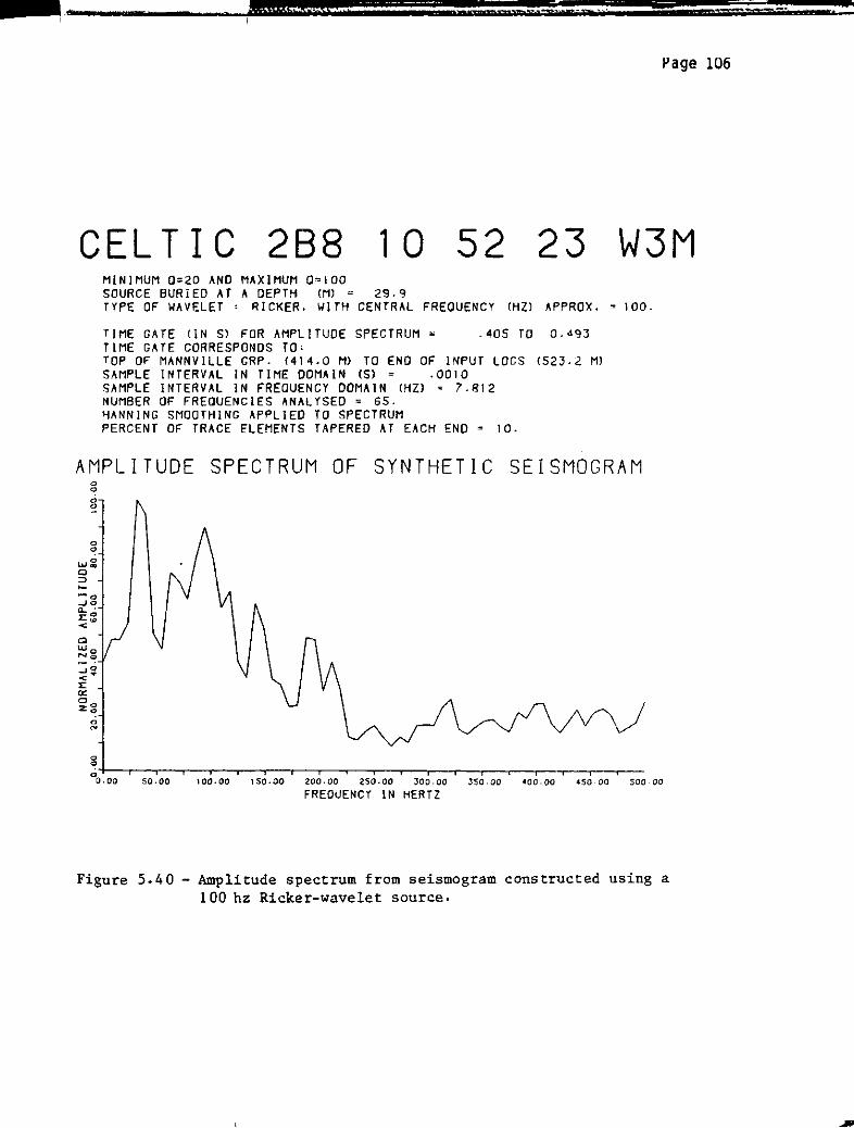
Page 106
CELTIC 288 1 0 52 23 W3MMINIMUM 0=20 AND MAXIMUM 0=100
SOURCE BURIED AT A DEPTH (M) = 29.9
TYPE OF WAVELET : RICKER. WI TH CENTRAL FREOUENCY (HZ) APPROX. 100.
TIME GATE (IN S) FOR AMPLITUDE SPECTRUM = .405 TO 0.493
TIME GATE CORRESPONDS TO:
TOP OF MANNVILLE GRP. (414.0 M) TO END OF INPUT LOGS (523.2 M)
SAMPLE INTERVAL IN TIME DOMAIN (S) = .0010
SAMPLE INTERVAL IN FREOUENCY DOMAIN (HZ) = 7.812
NUMBER OF FREQUENCIES ANALYSED = 65.
�ANNING SMOOTHING APPLIED TO SPECTRUM
PERCENT OF TRACE ELEMENTS TAPERED AT EACH END = 10.
AMPLITUDE SPECTRUM OF SYNTHETIC SEISMOGRAMo
o
o
a
100.00 150.00 200.00 250.00 JOo.OO 3S0.00 400.00 450·00 SOO·OO
FREOUENCY IN HERTZ
Figure 5.40 -
Amplitude spectrum from seismogram constructed using a
100 hz Ricker-wavelet source.

., ... ,., ... ,_.......- .. -��
5
,=;=,,-",
, I!
Page 107
CELTIC 288 1 0 52 23 W3MMINIMUM 0=20 AND MAXIMUM 0=100.
SOURCE BUR I ED A. T A DEPTH (M) = 29.9
TYPE OF WAVELET : RICKER. WI TH CENTRAL FREOUENCY (HZ) APPROX. 140.
TIME GATE (IN S) FOR AMPLITUDE SPECTRUM = .405 TO 0.493
TIME GATE CORRESPONDS TO:
TOP OF MANNV I LLE GRP. (414.0 M) TO END OF I NPUT LOGS (523·2 M)
SAMPLE INTERVAL IN TIME DOMAIN (S) '" .0010
SAMPLE INTERVAL IN FREQUENCY DOMAIN (HZ) = 7.812
NUMBER OF FREOUENCIES ANALYSED = 65.
HANNING SMOOTHING APPLIED TO SPECTRUM
PERCENT OF TRACE ELEMENTS TAPERED AT EACH END = 10.
AMPLITUDE SPECTRUM OF SYNTHETIC SEISMOGRAMo
n
o
o
o
n
o+-�--��--��--��--�-'--'--'--'--'--'--.--.--.�.--.r-,0.00 50.00 100.00 150.00200.00250.00 JOO.OO 350.00 400.00 450.00 500.00
FREOUENCY IN HERTZ
Figure 5.41 -
Amplitude spectrum from seismogram constructed using a
140 hz Ricker-wavelet source.

_-----tt-.....
,
it 'iEt; t
.
%' '!
Page 108
CELTIC 288 1 0 52 23 W3MMINUMUM 0=20 �ND MAXIMUM 0=100.
SOURCE BUR I ED AT A DEPTH (M) = 29. 9
TYPE OF WAVELET : �ICKER. WITH CENTRAL FREQUENCY (HZ) �PPROX. 178.
TIME GATE (IN S) FOR AMPLITUDE SPECTRUM = .405 TO 0.493
TIME GATE CORRESPONDS TO:
TOP OF MANNVILLE GRP. (414.0 M) TO END OF INPUT LOGS (523.2 M)
SAMPLE INTERVAL IN TIME DOMAIN (S) = .0010
SAMPLE INTERVAL IN FREQUENCY DOMAIN (HZ) � 7.812
NUMBER OF FREQUENCIES ANALYSED = 65.
HANNING SMOOTHING APPLIED TO SPECTRUM
PERCENT OF TRACE ELEMENTS TAPERED AT EACH END = 10.
AMPLITUDE SPECTRUM OF SYNTHETIC SEISMOGRAMo
(')
o
o
o<>
100.00 lS0.00 200.00 250.00 aoo , 00 J50·00 400.00 450.00 500·00
FREOUENCY iN HERTZ
Figure 5.42 -
Amplitude spectrum from seismogram constructed using a
180 hz Ricker-wavelet source-

_"·__�� -WJ�_J4M1I1;4�;'!:!!H�'!'!t�(:::::::::::::»:·:;;:;::sn:':D:··�;��;··:n:'�;:l:::::::;;:::::T70��.'�'��::::�!,.Ic=
)
Page 109
CELTIC 288 1 0 52 23 W3MMINUMUM Q=20 AND MAXIMUM a�loo.
SOURCE BURIED AT A DEPTH (M) = 29.CJ
TYPE OF WAVELET : �ICKER. WITH CENTRAL FREOUENCY (HZ) APPROX. = 222.
TIME: GATE (IN S) FOR AMPLI TUDE SPECTRUM = .405 TO 0.493
TIME GATE CORRESPONDS TO:
TOP OF MANNVILLE GRP. (414.0 M) TO END OF INPUT LOGS (523.2 M)
SAMPLE INTERVAL IN TIME DOMAIN (S) = .0010
SAMPLE INTERVAL IN FREQUENCY DOMAIN (HZ) = 7·612
NUMBER OF FREOUENCIES ANALYSED = 65.
HANNING SMOOTHiNG APPLIED TO SPECTRUM
PERCENT OF TRACE ELEMENTS TAPERED AT EACH END = 10·
AMPLITUDE SPECTRUM OF SYNTHETIC SEISMOGRAMo
o
o
o
o
UJoNO
....10<
...
1:Q:
�go'"
100.00 lS0.00 200.00 250.00 300.00 3S0.00 400.00 �SO.oo $00.00
FREQUENCY IN HERTZ
Figure 5.43 - Amplitude spectrum from seismogram constructed using a
220 hz Ricker-wavelet source·

W'WI,! £J "{' ;t i:::
Page 110
portions of the seismograms in Figures 5.4 and 5.33 are probably as a
result of interference from the side lobes of the Ricker wavelet. The
seismogram in Figure 5.33 is also delayed, due to the linear-phase
characteristic of the Ricker wavelet.
The choice of filter used in synthetic seismogram construction or
seismic processing is important. The filter of 80 hz peak frequency
provides the most realistic response from the Mannville section because
it most closely imitates the (anti-alias filtered) impulse response. If
a low-frequency filter is used (for example, one corresponding to the 60
hz wavelet in Figure 5.32), the lower frequency portions of the
amplitude spectrum are increased relative to the higher frequency
portions and important, high-frequency reflections from the Mannville
may be destroyed. If a high-frequency filter is used (for example, one
corresponding to the 100, 140, 180, or 220 hz sources of Figures 5.34
through 5.37), the higher-frequency portions of the spectrum are
increased relative to the lower frequencies and the important,
high-frequency reflections will be accentuated.
For thi s study, however,
the best choi ce is the impul se source.
This is because the impulse source is zero phase and contains all
frequencies in equal proportions (Sheriff, 1973). Thus, the impulse
response seismogram shows how all of the sampled frequencies (that is,
within the theoretically available range of frequencies that is
determined by the sampling rate) have responded to the filtering of the
simulated earth-model.
5.4 Variation Among Wells
Usi ng the "best" input parameters--an impul se source bur; ed at 29.9
m and the standard Q-function, as were chosen from tests on well 288 in

r-w M"?MJ m' I
'Z'Z":m=- ,!
Page 111
section 5.3, synthetic seismograms were constructed for the
pilot-project wells and well 4-11. The synthetic seismograms for these
seven wells are shown in Figures 5.44 through 5.50. The amplitude
spectra for all seven wells are shown in Figures 5.51 through 5.57.
The Mannville portions of the synthetic seismograms of the six
pilot-project wells are not markedly different from one another. The
cross-section in Figure 4.5 has already pointed out the geological
similarity among the six wells; consequently, the similarity of their
synthetic sei smograms is not surpri si ng. Still, there are si gni fi cant
differences among the seismograms. A synthetic seismogram cross-section
through the pi 1 ot-proj ect we 11 s, v/hich is fl attened on the top of the
Mannville Group, is shown in Figure 5.58. Although the Colony gas-zone,
McLaren coal-bed, and Waseca oil-saturated-sand zones reflected
responses are visible in each seismogram, the relative sizes of the
waveforms vary significantly.
The response of well 402 is most different from the others. In
comparing the Mannville portions of the synthetic seismograms, the
frequencies in well 402 (Figures 5.46 and 5.58) are distinctly higher.
Whereas the amplitude spectra of the other five pilot project wells have
dominant frequencies of 40 hz, well 402 (Figure 5.53) has a dominant
frequency of 93 hz, the entire range of 55 to 95 hz being over 95 per
cent of the peak amplitude. The most probable cause of these high
frequencies is found within the Colony gas zone. In well 402, the low
acoustic impedance gas zone is interrupted by a thin high velocity and
density (probably calcite cemented) bed. Due to this zone of high
acoustic- impedance, the normally large and broad 40 hz gas-peak is
split into two high-frequency peaks and a trough. The measured
frequency of these waveforms is approximately 80 hz. From a few ms

1

_ICELTIC 202 1 a 52 23 W3M
0 DENSITY VELOCITYSYNTHETIC STRATIGRAPHICSEISMOGRAM MARKER BEDS
a KG/CUBIC METRE -rc' METRES/S _'02 AMPll lUDE _, 02
od.OO 40.00 '0.00 0'50.00 200.00 250.00 .,10.00 30.00 50.00 .,-60.00 -30.00 0.00 30.00
·r�n"",,'o ., g ..,
g -nIDPLE ORlfI" 0 0
·lOIlER DRIFf
... ... ... ... ..
0 0 <> <>� .
NOM (AllA GROUP
u (, (, g - 05 , g nof' or L(A PARPI fn.'0 0 <>
0 ;; ;; ;; ;;0 .., <> <>
�.., s g g -
.10 S ..,
.., o
i;; ;; ;; ;;; ;;;<> <> <> 0 0
.., g g g .- .IS , g..,
'" '" ... '" ..
<> 0 <> <> <>
o 0 '" 0 <>
.., .., 0 g -
.20 S s<> 0 <>
0 0 0 0 c
rn ", ,.. ,..
!:l .. I -u. rOlORAOO r.Rour-0" -U ... " ... -0 ..
_, .... � ... ...... ...... .... ...
x? :I:� :I:� :I:� :I:�v 0
_g _gi
sJ: f�Pr::r&Up�rf.fi�b�o
�II·�o _0-. Z5 ,
z :z: :z: :z:
3 ....
�g::I'" 3'" 3'"
rno ",0 ,..0 ",0
--.? ...... .....0
..... � .... ?::Uu ;00 ;00
�g � g
�-lor sr . IIAlBURr. S�I
",<> .... 0 ,..0'" .." .." .."
- .30 S .."SAGE &I. IIA18URr. "' .
... ... ... ... ...
'" ... .. .. ...
0 0 0 0 0
(.) 0 0 .., (,<> .., <> 0 0
-
. lS S
H �A .. ..
!;A
<> 0 0 ..,
0 0 .,
�1m_..", '"-
I ;, .. o
.., 0 ..,.
""UREN fn·
H I �i � �i } �i.4H
....
"AsrCA 'H.
..
? "'"'�'tlU rH·
e>
0
C[HERAL rEIROLfUltS rlt.
HI
;1e=_
:1f
l<:
'".·RU fit·
0
<>
<>
<>
�J �J �J ""tJ
g}0 0 0 0 c»
CO0 0 <> e 0
C1)
Figure 5.45 - Well logs and synthetic seismogram for well 2D2.......
......
w
�
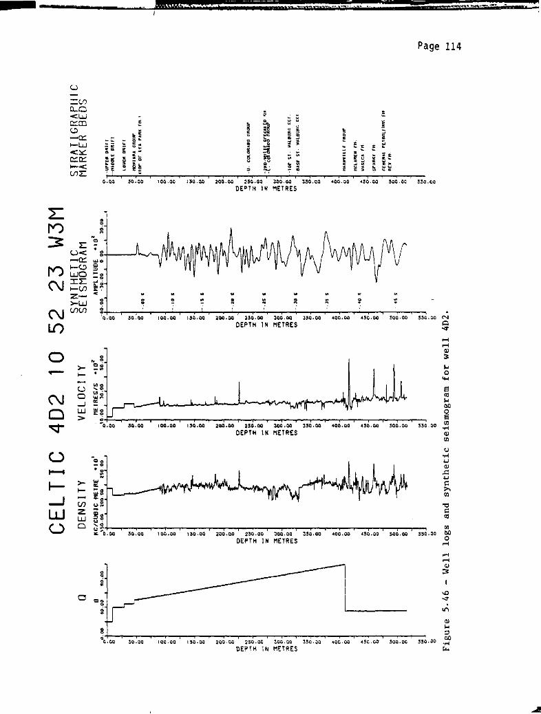
ICELTIC 402 1 0 52 23 W3M
0 DENSITY VELOCITYSYNTHETIC STRATIGRAPHICSEISMOGRAM MARKER BEDS
0 KG/CUBIC MEIRE .'0' METRES/S ., 02 AMPlI TUDE •• 02
��o}'>O.OO 100.00 no.oo 0'°·00 30.00 50.00 0-60.00 -30.00 0.00 30.00
� -UPPER PRIH0 0 (,0 0 0 s
}"'"''"'"
'lOIl{N PRlr •
'" .. '" ..
0�
0� '""MIANA GROUP
(, 0 0
g (lOP or lU PARK rlt.'0 0 o ·-.05 &;
H \;; (; (; (;0 0 0 0
g (, s -"0 S0
0 0
;1 \;; ;; c:; c:;0 0 0 0
0 s g - .IS &; g0
., ., N
g.,
0 0 0 0
0 0 0 0
o (, g g -.20 S0
0 0 0
t:I t:I 0 0 t:I
f'l f'l f'l f'l f'l
11., "N "N ".,! t: I -u· COLORADO r.RaUl'
...... ......'" ..... '" -t'"
:r� :r? :r!' :r? :z?., 0
-g0 0
_0 _0 _0-.25 , �
0
i -f"O-I['AU 'r�m,o�".
;e :z :z :z-
. CO 110 ."OU
3'" 3'" 3'" :I .... 3'"
f'lo f'lg f'lo f'lo f'lo...... !' ...... -
.... ? ......C> .... !'
;1)0 ::00 ::00
�g � s
�-101' SI. IIALBURG ss r .
f'lD f'lo f'lo." tn (I) tn
- .lO S (I).
Bur u. IIAlBURG SSI
... ... ... ... ...
'" .. III .. '"
o· 0 0 0 0
... g g g0
b b
... JS S
H \. . .
g0 0 0
0 0 0
I s (, (,
T''''''''-0 0 0
IICLARE" rlt.
�1... . ...
-·.0 II;
:;. ""SEC", fl1·'" '" '"
0 0 0 0
0 s 0 g -SPARKY fit.
a 0
r.UERU PE'ROlfU"� Fit.
'" '" '" '" Rn rll·0 a a
. 4S S0
0 a 0 0
g s0 g0
lA
'"
o·
.,
o
::o
o
o
'"
'"
o
o
o
"'0
III
to
(1)
Figure 5.46 - Well logs and synthetic seismogram for well 4D2. .....
.....
.,::..
�

17
....." ..
......
::r?o
_0
2!
3t;�o;110.....
0
'"
o
o
00.00 40.00 80.00
oI ,
• , •
o
CELTIC
DENSITY
KG/CUBIC HErRE -'01
01S0.00 200.00 150.00
If't ,
gI
..
o
g-'
g
g
i;o
g
0>
..o
go
.....
"0>..... ..
::r0
_8z
�g......
�gen
t:..
g
...
g
g
�o
g
�o
g
..
..o
g
288 10 52
..
o
g
oo
8
..
o
oo
.,
g
g
...
o
o
g
23 W3M
..
..
o
g
..
<>
o
<>
<>
..
'"
o
C
METRES/S _102010.00 30.00 50.00
I I ' , I
gI
SYNTHETICSEISMOGRAM
"HPll TUDE • '0'0-60.00 -30·00 0·00 30.00
• J' , e
I' ,
g
VELOCITY
z
t:<>
g
z
...
D
g
..
D
g I--.os S
ig
i• g.-.Ios
i
8
i;o
g.-.15S
�<>
..D
o
'"
!f:XO
_8
g81.-.105
o
....
" ..
.......
x?
_8
�g......
�gIn
��.....
0
;II'..... 8en
tg
1
-.35 C
g..
�j
..
t...
i- .�O s
...
0
8
g l-·'s S
;,0
Figure 5.47 - Well logs and synthetic seismogram for well 2B8.
�
-.as Ii
-.lO C
STRATIGRAPHICMARKER BEDS
!'l-Wf£IIIIll1n
g -niIlOlE Olliff
-lO\l£II PIIlff
...
!'I-noll
JAil' IlllOUl'
g' "Of or lEA 'AIIII rH.'
g
g
i;o
g
g8
o
PI
� �.J -Cl. COlDIIAOO GIIOUI'
-gz
l:l�lIilrm08r�filUosn.
3�"'0.....
;IIg� J
- for Sf. VAlIIlJRC SSf.
t:I-eas[ Sf. VAllIUftC SSI.
(>
8
gg l-nAtllI' IHE 1111001'
-HCUII£II rH.
..
f1-VAS[CArH·
o -$PAftllf rH.
� I �:�:£�!�rEI"utrum; rH .
o
g
...
..
o
g
_I
\:J
�
(Q
(J)
.....
......
01

o
m
-"",
-t ....
:r?o
_0
:z
3 ....
mO-to;Ua,..,0.n
o
o
00.00 fO.OO eo.oo
.,4--�--4---��-o
....
o
o
.,
CELTIC
DENSITY
KG/CUOIC METRE -10'
o'SO.DO 200.00 250.00
(;,I
I ,
"
,
.,
g.,.,
oo
.,
.,
...
.,
.,
e»
...
.,
.,
go
'"
" ...
-t'"
XO
-g:z
�g--to
�gVI
gg
..
..
o
g
..
s
s
488 52
o
o
o
o
..
.,
o
o
IV
o
o
o
o
...
..
o
o
o
..
o
o
c»
<>
..
...
.,
g
..
<>
o
o
.,
..
...
.,
<>
<>
10 23 W3M
VELOCITYSYNTHETIC
SEISMOGRAM
METRES/S _102 �MPLI TUDE _102
0'°·00 30.00 50·00 .,-60.00 -30.00 0.00 30.00
Q <><> 0
... ...
<> 0
Q .,.,
: tos5
00 g
Q g .-.'0 C0
;; ;;.C> <>
g g �-.,S C
... ...
<> 0
0 <>
g g h20 C
0 0
,., ,.,
" ... ,,'"
-t'" ..... ...
X� :x:�
_8 .... g�-.ass:z :z
:1:'" :1:'",.,0 ,.,g-t? --to
�g::00
,.,0VI VI J.- .JO S
...t:..
0 0
g 0
0
i· .J5 S
.. ..
., .,
0 0
s g
.. .. 1-.405
.. ..
., 0
g s
...
...... - 45 S..
o
.,
...
...
.,
s
to
'"
.,
C>
o
Figure 5.48 - Well logs and synthetic seismogram for well 4B8.
�
STRATIGRAPHICMARKER BEDS
? -urrER DRI,'
g 1· H'DPLE ORIr!
...
oo
g
-lOIlEIi ORIH
'"
o
i-1IO"IANA GROUP
g 1101' 0' lU fARK 'H·I
o
<>
s
to
o
.,
.,
o
f'l
" ...
-t'"
x?
_ g • -u. COl ORAOO GROUP
z
� l=f�DtXrmDfil'mb�"�H.
....
;U
ITI
(/)
'UP SI. IIAUIU,." S�I.
� J -IIASE 51. IIAlIIURG 551 .
g
..
oo·
.,
.,
.
HAHH¥ ILl[ GROur
�it1ClMIU rH·
g·IIAsrCA 'H.
,,.ORKI rH .
'UERAl I'HROlfUH� 'H·
RU 'H.
J
"
IlJ
(0
f1)
......
......
0'1

ICELTIC 208 1 0 52 23 W3M
0 DENSITY VELOCITYSYNTHETIC STRATIGRAPHICSEISMOGRAM MARKER BEDS
0 I<G/CUBIC METRE -101 METRES/S _'02 �MPLI TUDE _, 02
00.00 '10.00 10.00 .,150.00 200.00 ZSO.OO 0'0.00 30.00 50.00 0-60.00 -30.00 0.00 30.00
'rw""�'"
gl t=:! I !
glI
1,::1'I I
giLl', , , ,
g 1I ' I
I, , ,
g 'HIOOlE ORlff
··lOliER ORlff
;1 \VI VI VI
�VI
0 0 0!' -ttO"r AliA GROIlP
0 0 g g 1I0f OF lEA PAliK FH.'0 ., -.OS'
g g0 0., 0
0 <> g-
.10 S <>0 0 0
;;; ;;; ;;;
:1 \..
0 0 0 0
<> <> g- .15 C <>
0 0 0
'" ... ... ... .,
0
g0 0 0
0 0 0 0
<> 0 <> g "0 0 0
-.20 s0
0 0 c c 0
m (1'1 (1'1 (1'1 fTI
"., -U ... " ... " ...
! � I U. COLORADO CROUP.... '" _lO ....... ..... ..
:r? :r? X? X? 7.
... ., 0 0- .as ,
0
�o .... 0 _0 _0 _0
z :z :z z z
3'" 3'" :I'" 3'" :I'"'
mg .... g .... g .... g � g1-fHD-Wrl�E SfmlJO'N·..... . ...
. ..... .... .
i!:3:Uo :Uo :Uo ;:u <.
-
. CO 0 ADO CROU
.... 0 fTlO .... 0- .lO S
fTlOVI (J) en en (J)
... ... '" ... ...
lO lO VI VI
:;
i-rapsr . IIAleupro SSI
0 0 0 0
0 0 <.s
" BASE sr . "ALUIIRC 55!.0 0 ., 0
-. JS S
...
g g g..
'0 0
0 .,
<> ., <> <> <>
o 0 0 0 0
'.40 S
... ... ... ...
=}:; HAHHYlll[ cRour'" VI '" o.
0 <> <> <>? -HCLAREN fH·
;, <> <> 0 <>
., ... <> <> <>
"ASECA FH.
:1 I :1 �'" '" -.45 S VI
<> 0
g.
SPARKr rH.0 <>
... t>
g -C[NERAl fElIIOlfllHS 'N.0 0
REX rn·
o. ..
-0.. ..
<> o
g,
s<> C> C>
to<> e> 0
tl)
Figure 5.49 - Well logs and synthetic seismogram for well 2D8.......
......
.......

o
111
-U'"
...'"
::J: ?°
_0
:z
3 ....
111°-fo;:0o1110<n
a
o
00.00 40.00 80.00
Q' r' • ,
o
o
o
oo
DENSITY
KG/CUBIC MElRE e'OI
OISO.OO 200.00 250.00
I« , « , «
(:,.
o
...
o
.,o
o.,
o
.,
..
.,
g
o
111
"11 ..
_,,,,
x�.,
_0
z.
��....
0
;;0o1110(11
...
<II
o
o
o
.
.,
o
s
.
..
o
g
...
oo
<>
<>
4
..
oo
go
'"
"11'"
......
XO
_g
�g;';0",0(IJ
1 1 52 W3MSYNTHETICSEISMOGRAM
AtlPLI TUDE -, 02
.,-60.00 -30.00 0·00 JO.OO
Uo
23
..
VI
o
p
<>
'"
o
o
o
VELOCITY
MEJRES/S a,O'010.00 30.00 50.00
I« « , t
gi
..
o
oo
o.,
.,
o
..
o
g J -", 05 ,
.,o
U J-.IO ,o
..
.,
o I .. IS Co
'"
<>
0
g �. ·lO S
0
'""11"
_,,,,
X�
_g�-.lS':z
3'"",0.... �;;00
",o.-.lOS(I)
'"
<II
<>
0
0
-t-JS ,
.
0
0
g
i- .40 S
t-o
<>
.,
� 1-· 4S S.,
(.)
0
Figure 5.50 - Well logs and synthetic seismogram for well 4-11.
�
<II
<>
o
o
..
oo
g
....
<II0_
...
o
.
o
o
o
o
..
<>
s
..
o
0-
g
..
..
o
s
..
o
oo
:z
...
<II
<>
<>
.,
.
o
<>
g
IA
o
g
..
<>
<>
<>
<>
STRATIGRAPHICMARKER BEDS
<>
g r�:��c'I:!��,
oo
s
IIASHA fit.
SrAR�' III·
lOUfR ORlff
..
? J MONI ""A GROUr
g I liar or lEA PARK 'M.)
..
o.
o
<>
'"
o
o
(,o
o
m
,,'"
... ...
:x�
_ g I.
u. COlORAao GROUr
:z
� tll-2ND-lIlflIE SrECKlED Sit.
....0 -t -t . COLORADO r.ROI)P
;;00",0In
tl,-lor SI· IIAlPURG sst
.,
<>
.,
IIASE SI. "'lBURG SSI.
.
oo
"
(>
ItA""Y IUE GROur
••IICLAREH 1M •
..
o
g
..
giCUFRAl rEIROlfUH& rlt·
e, flU rlt.
<>
)
-0
III
(,Q
(1)
.......
.......
00

AN1.!!: it; w de£
Page 119
CELTIC 4B2 1 0 52 23 W3MMINIMUM 0=20 AND MAXIMUM 0=100
SOURCE BUR I EO A T A DEPTH (M) = 29.9
TYPE OF WAVELET: IMPULSE
BUTTERWORTH ANTI-ALIAS FILTER INCLUDED IN SYNTHETIC TRACE
TIME GATE (IN S) FOR AMPLITUDE SPECTRUM .374 TO 0.443
TIME GATE CORRESPONOS TO:
TOP OF MANNVILLE GROUP (402.2 M) TO TOP OF REX FM. (482.3 Ml
SAMPLE INTERVAL IN TIME DOMAIN (S) = .0010
SAMPLE INTERVAL IN FREDUENCY DOMAIN (HZ) = 7.812
NUMBER OF FREOUENCIES ANALYSED = 65.
HANNING SMOOTHING APPLIED TO SPECTRUM
PERCENT OF TRACE ELEMENTS TAPERED AT EACH END = 10.
AMPLITUDE SPECTRUM OF SYNTHETIC SEISMOGRAMo
o
o
o
100.00 i50.00 200.00 250.00 JOO.OO J50.00 400.00 450·00 500.00
FREOUENCY IN HERTZ
Figure 5.51 - Amplitude spectrum from seismogram for well 4B2.

M!.4i4' tM ,; ,« i::
Page 120
CELTIC 202 1 0 52 23 W3MMINIMUM 0�20 AND MAXIMUM 0=100
SOURCE BURl ED AT A DEPTH (M) = 29.9
TYPE OF WAVELET : 1 MPULSE
BUTTERWORTH ANTI-ALIAS FILTER INCLUDED IN SYNTHETIC TRACE
TIME GATE (IN S) FOR AMPLITUDE SPECTRUM .374 TO 0.444
TIME GATE CORRESPONDS TO:
TOP OF MANNVILLE GROUP (404.5 M) TO TOP OF REX FM. (484.3 Ml
SAMPLE INTERVAL IN TIME DOMAIN (S):o .0010
SAMPLE INTERVAL IN FREQUENCY DOMAIN (HZ) = 7·812
NUMBER OF FREOUENCIES ANALYSED = 65.
HANNING SMOOTHING APPLIED TO SPECTRUM
PERCENT OF TRACE ELEMENTS TAPERED AT EACH END � 10.
AMPLITUDE SPECTRUM OF SYNTHETIC SEISMOGRAMo
c>
<>
o
o
WoNo
:;0<
....
1:0:::
�go
N
100.00 150.00 200·00 250.00 JOO·OO J50.00 400.00 450.;:10 500·;)0
FREOUENCY IN HERTZ
Figure 5.52 -
Amplitude spectrum from seismogram for well 2D2.

'�):H··_ .•
--,-tt &a4';'S" 'fit.1
::
Page 121
CELTIC 402 1 0 52 23 W3MMINIMUM Q�20 AND MAXIMUM Q=IOO
SOURCE BUR I ED AT A DEPTH (M):: 29.9
TYPE OF WAVELET: IMPULSE
BUTTERWORTH ANTI-ALIAS FILTER INCLUDED IN SYNTHETIC TRACE
TIME GATE (IN 5) FOR AMPLITUDE SPECTRUM = .379 TO 0.446
TIME GATE CORRESPONDS TO'
TOP OF MANNVILLE GRP. (409.') M) TO TOP OF REX FM. (488.4 M)
SAMPLE INTERVAL IN TIME DOMAIN (S):: .0010
SAMPLE INTERVAL IN FREQUENCY DOMAIN (HZ) :: 7.812
NUMBER OF FREQUENCIES ANALYSED = 65.
HANNING SMOOTHING APPLIED TO SPECTRUM
PERCENT OF TRACE ELEMENTS TAPERED AT EACH END = 10.
AMPLITUDE SPECTRUM OF SYNTHETIC SEISMOGRAM"
"
"
"
CI
W"No
::;0<.L
ct::
�g"
'"
"
"
,,+--Y--��--��--.-�--.-�--��--'-���������-'r-�0.00 50.00 100·00 150.00 200.00 250.00 JOO.OO :lSO.OO 400.00 4S0.00 sou.uo
FREQUENCY IN HERTZ
Figure 5.53 -
Amplitude spectrum from seismogram for well 4D2.

ISs
Page 122
CELTIC 288 10 52 23 W3MMINIMUM 0=20 AND MAXIMUM Q�IOO
SOURCE BURl EO AT A DEPTH (M) = 29.9
TYPE OF WAVELET: iMPULSE
BUTTERWORTH ANTI-ALIAS FILTER INCLUDED IN SYNTHETIC TRACE
TIME GATE (IN S) FOR AMPLITUDE SPECTRUM .405 TO 0.471
TIME GATE CORRESPONDS TO:
TOP OF MANNVILLE GRP. (414.0) TO TOP OF REX FM. (492.Q M)
SAMPLE INTERVAL IN TIME DOMAIN (S) = .0010
SAMPLE INTERVAL IN FREQUENCY DOMAIN (HZ) = 7.�12
NUMBER OF FREQUENCIES ANALYSED = 65.
HANNING SMOOTHiNG APPLIED TO SPECTRUM
PERCENT OF TRACE ELEMENTS TAPEREO AT EACH END = 10.
AMPLITUDE SPECTRUM OF SYNTHETIC SEISMOGRAMo
<>
o
o
o
<>
o+-�--��--��--.--'--.--'--���-r��-r�.--r--r--r--r-�0.00 50.00 100·00 150.00 ZOO.OO 250.00 300.00 3<;0.00 400.00 450.00 SOO·OO
FREOUENCY IN HERTZ
Figure 5.54 - Amplitude spectrum from seismogram for well 2B8.

"'01,; .. n ..
-_,-- I:::::
Page 123
CELTIC 488 10 52 23 W3MMINIMUM Q=20 AND MAXIMUM Q=IOO
SOURCE BUR I ED A T A DEPTH (M) == 29. q
TYPE OF WAVELET : IMPULSE
BUTTERWORTH ANTI-ALIAS FILTER INCLUDED IN SYNTHETIC TRACE
T I ME GA TE (l N S) FOR AMPLI TUDE SPECTRUM .394 TO 0.459
TIME GATE CORRESPONDS TO:
TOP OF MANNV I LLE GROUP (427.5 M) TO TOP OF REX FM. (506.5 M)
SAMPLE INTERVAL IN TIME DOMAIN (S) = .0010
SAMPLE INTERVAL 1 N FREQUENCY DOMA I N (HZ) " 7.812
NUMBER OF FREQUENCIES ANALYSED == 65.
HANNING SMOOTHING APPLIED TO SPECTRUM
PERCENT OF TRACE ELEMENTS TAPERED AT EACH END == 10.
AMPLITUDE SPECTRUM OF SYNTHETIC SEISMOGRAMo
o
o
o
100·00 150.00 200.00 250·00 JOO.OO 350.00 400.00 450.00 500.00
FREOUENCY IN HERTZ
Figure 5.55 -
Amplitude spectrum from seismogram for well 4B8.

eN:d: 11:;1
,
Pagg 124
CELTIC 208 1 0 52 23 W3MMINIMUM Q�20 AND MAXIMUM Q=100
SOURCE BURIED AT A DEPTH (M) = 29.9
TYPE OF WAVELET : 1 MPULSE
BUTTERWORTH ANTI-ALIAS FILTER INCLUDED IN SYNTHETIC TRACE
TIME GATE (IN S) FOR AMPLITUDE SPECTRUM .414 TO 0.479
TIME GATE CORRESPONDS TO:
TOP OF MANNVILLE GROUP (443.3 M) TO TOP OF REX FM· (523·2 M)
SAMPLE INTERVAL IN TIME DOMAIN (S) = .0010
SAMPLE INTERVAL IN FREQUENCY DOMAIN (HZ) = 7.812
NUMBER OF FREOUENCIES ANALYSED = 65.
HANNING SMOOTHING APPLIED TO SPECTRUM
PERCENT OF TRACE ELEMENTS TAPERED AT EACH END = 10.
AMPLITUDE SPECTRUM OF SYNTHETIC SEISMOGRAMo"
o
o
oC)
w�o
::>,_
-0...10
0..'
I:�<
o
WoNO
::;0<..-I:
0:
�go
'"
o
o
o+-�--�-'--T-�--��--�-'--'--'--'--'--'--'--'--'--'--'--'0.00 50.00 100.00 150·00200.00 250.00 300.00 JSO.oo 400.00 4S0.:J0 500·00
FREaUENCY IN HERTZ
Figure 5.56 -
Amplitude spectrum from seismogram for well 208.

Page 125
4 1 1 52 23 W3MMINIMUM Q=20 AND MAXIMUM Q�IOO
SOURCE BUR I ED A T A DEPTH (M) = 29.9
TYPE OF WAVELET : 1 MPULSE
BUTTERWORTH ANTI-ALIAS FILTER INCLUDED IN SYNTHETIC TRACE
TIME GATE (IN S) FOR AMPLITUDE SPECTRUM .396 TO 0.462
TIME GATE CORRESPONDS TO:
TOP OF MANNVILLE GROUP (425.5 M) TO TOP OF REX FM. (406.8 M)
SAMPLE INTERVAL IN TIME DOMAIN (S)'" .0010
SAMPLE I NTERV AL I N FREQUENCY DOMA I N (HZ) = 7·812
NUMBER OF FREQUENCIES ANALYSED'" 65.
HANNING SMOOTHING APPLIED TO SPECTRUM
PERCENT OF TRACE ELEMENTS TAPERED AT EACH END'" 10.
AMPLITUDE SPECTRUM OF SYNTHETIC SEISMOGRAMo
C)
o
o
o
WoNt?
...JO
<:...
E
�
°020
Figure 5.S7 -
Amplitude spectrum from seismogram for well 4-11.

." ......"T"" .,,'
't U t:.1-.11.1 4 B 8
208
; I
.
, -,�.oo, 0.00! 'OjOO ",-60.00 A!1!o��OTUDE
0102AMPLI TUDE
2
£:.. U u
I.
0.00
olD
,
.,U '.00
...."T"'"' .,,' .,,'
,"pcrr"" .,,'-sc.cc
,"PC""" • .,r
-'to_0 • O�'l'l'o.oo�'
a -'0.00 0.00 'O.OO�-30.00 0·00 30·00
_L __ .I. _D
04B2
�L05 •
..
0
"o �-,05 ,
0 (;0 0
8-.10 S g "-.10 S
'" ;;;0 0
g-
.1$ .. g 1--.15 ,
'" '"
0 0
" 0
g -
·20 S g�-'20Sa
'"
-0 ... '"
--<'" ..
:r?0
0 0
_0-,25 S "�-,25'
:z:
3 .... ....
",0 0
...,0"
::00 "",0
-
,lO S
0
.J.-,30 •In
t:....
..
" 0
" s0
-,'5 ,1-,'· ,
�0
0
0
-.40 C
�...
1-.40 ,
'" '"
0 0
s"0
'" '"
g -.45" g �-.4S ,
0 g0
'" '"
.. ..
0 0
s g
2022BQ
..
0
gt-·os£
IL- 10'
10..
0
's r-. IS ,
'"
0
0
g 1-- .20 S
''''
'"
"
g�-'2s,
....
0
'0
"
: -t-'0 S
'"
0
g
..
1-,'5'0
0
gI
-,10 S
._
�t-- 45 s
0
s
'"
..
0
g
�LoSG J=-..
'"
0 L?
0
0
o -.Os,
o�-,oss
H- 10 S �(; �
(;"
0 g 1--.10 ,
g -_.0'
'"
..
..
0
0
's -·15"
0 g hIs,
g -.IS Ii
g..
'"
0
0
0
"
0 g �-,20 ,
o -.20"g -.,0 Ii
�..
'"
'"
0
..
?
"
0
;,
0
0-
,2$ ,
o -.2S'
" �-,2. ,
...
..
...
0
�
0
..
"
..
;,
0
..
0
-.30 s
..
-·30 ,
.J.-,30 ,
...
...
...
'"
'"
"
..
?
"
..
g
0
Q
0
-, ,. s
-.15 ,
1--.'. ,
�
�Q
.. g-- - --& -----
-.40 ,
�-
·10 ,
... 1--.40 s:
'"
..
(II
"
?
s
..
;,
0
Q
0
'"
g-J.- .45 ,
g -.45 sIi
- .45 C
g;,
"
..
Q
'"
..
'" tg
0
'" gg
'"
Figure 5.58 -
Synthetic-seismogram cross-section, flattened on the top of the Mannville Groupo
'tI
J
""Q
QI
to
I'D
.
N
0'\

'dUg "i 4i, i ;,..,.....-
Page 127
above the gas-zone peak (due to the zero-phase characteristic of the
impulse source) to the end of the seismogram, the higher frequencies
predominate. The importance of the gas zone to the Mannville portion of
the synthetic seismogram will be discussed further in chapter six.
The McLaren formation coal-bed response varies somewhat from well
to well but is always distinctly visible. In wells 4B8 and 208, the
coal bed response is seen even though the low density character of the
beds is very poorly developed. Therefore, the coal bed response is not
solely a result of the presence of the coal bed; interference with some
other reflection must be accentuating this response.
The opposite situation is seen with the reflections from the WI
cemented-zone. In all six wells, the response is as described for well
2B8 in section 5.3.2. That is, the WI reflected response is not
visible; it is obscured by interference from a larger trough occurring
at the same time. Even in well 202, where there is no cemented zone at
the base of the Waseca formation, this large trough is very similar to
that of the wells where the cemented zone is present. In well 402, a
small waveform is visible just below the larger trough. This may be the
WI zone response; modelling of the cemented zone could test this
hypothesis.
Responses from the W6 oil-saturated zone vary from almost
undetectable in well 402 to very large in we l l 2D8. Since the W6 zone
is only 3 to 4 m thick, its response is weak and interference effects
can either accentuate or nearly destroy the reflection.
The response from the W3 oil-saturated zone is clearly visible in
all of the six wells. The W3 zone is about 5 or 6 m thick, but for the
same reasons as for the W6 zone, its response is somewhat variable.
The Mannville geology of well 4-11 is different from that of the

BH;""!: ti,';"'Q'"
..P-;:,- .*- ...
Page 128
the pilot-project wells (see section 4.1); thus, the resulting
seismogram (in Figure 5.50) is particularly distinctive. The gas, MC,
W6, and W3 peaks cannot be picked with confidence. Core control in well
4-11 is poor. The W6 and W3 beds cannot be distinguished on the
geophysical logs and are likely not present in the well. There is a
high-velocity zone at the base of the Waseca formation and although
there is no core for verification, this zone will be called WI. A
high-frequency trough, which is likely the response to the cemented
zone, occurs at about 0.43 s. Three low amplitude, high frequency peaks
are visible between about 0.41 and 0.42 s. These may result from thin
oil-saturated sands in the McLaren formation.
If the 4-11 seismogram is shifted up in time by about 15 ms with
respect to the 2B8 seismogram, the portion of these seismograms below
0.3 s are more similar than they were before. However, the Mannville
formational boundaries no longer correlate. This means that the
well-log markers in well 4-11 may not have been correctly chosen, which
is possible in a well with poor core control and no density log. The
other noticeable effect of shifting the seismograms is that the W6 and
W3 peaks of well 2B8 now correspond to one large peak in well 4-11.
This is significant because it suggests that, in moving from a well
produci ng from the Waseca forma ti on to a we l l that does not produce from
the Waseca, the oil-zone reflections may change from a high frequency
doublet to a low frequency singlet. This is also what the synthetic
seismogram of Figure 5.3 showed when the Waseca oil zones was
artificially shaled out. Unfortunately, the core and log control in
well 4-11 is poor. It woul d be useful to repeat thi 5 test ina fi el d
where a dry well of known geology is located next to a producing well.

'*9M'5 i , i i If ,4 " \;' a"-
.--,.-... -
=. ,..,.,.rmw 7
:
"-C""I
Page 129
CHAPTER SIX
INTERPRETATION
6.1 Resolution Limits
When two or more geologic interfaces are located at a time spacing
less than the duration of the of the seismic pulse, their reflections
will be so close together that they will interfere. As the interval
between the reflecting interfaces decreases, there will be less
information from each of the individual reflections and more information
from the combined reflections, or wavelet complex. Resolution is the
process of separating reflections that are very close together, and
resolving power is the ability to distinguish between the properties of
these reflections (Widess, 1973). In contrast, the layer as a whole may
be considered, instead of just the two reflecting surfaces of the layer.
The threshold of detectability can then be defined as the minimum
thickness that a layer must have in order to produce a visible
reflection (de Voogd and den Rooijen, 1983).
Vertical resolution has been studied from different viewpoints by
several authors in the past thirty years. Rayleigh chose a spacing of
half the breadth of the main lobe of an optical diffraction-pattern to
be the separation necessary to resolve the diffraction patterns (Jenkins
and White, 1957, p. 299-301). Ricker (1953b) studied the resolving
power of two velocity-type Ricker-wavelets of equal amplitude and
polarity and determined that these wavelets were resolved at spacings
greater than 0.428 of the wavelet breadth. Widess (1973) investigated
the change of shape of the composite waveform produced by the
interference of two zero-phase reflections, of equal amplitudes and
opposite polarities, that were reflected from a progressively thinning

1 f§W2 I :1$ 4 I, : ;:no
.. a_'"
a ,!!
Page 130
bed. He chose the limit of resolution to occur at one eighth of the
predominant period of the incident wavelet, where the predominant period
is the breadth of the central lobe of the waveform. Schoenberger (1974)
concluded that zero-ohase wavelets have better vertical resolving power
than do minimum-phase wavelets. Koefoed (1981) proposed that the
aspects of the breadth of the central lobe, the side-lobe ratio, and the
amplitude of the side-tail oscillations together controlled the
resolving power of the seismic wavelet. Most recently, Widess (1982)
derived a quantitative formula (expressed by the variables of time,
waveform, and signal purity) for the vertical resolving power of a
seismic exploration system.
Of the above resolution concepts, that of Widess (1973) has been
most commonly used by exploration seismologists. By graphical means,
Widess observed that at a reflector spacing of less than one eighth of
the predominant period of the incident wavelet, the shape of the
composite reflection from the two interfaces of a thinning bed
stabilized to a reasonable approximation of the time derivative of the
incident wavelet. He defined the theoretical threshold of resolution to
occur at that point. However, he qualified this by adding that, in a
practical situation, other factors are also involved in determining this
threshold. These factors include the presence of noise, the form and
duration of the incident wavelet, the degree to which the wavelet is
known prior to the analysiS, and the analytical tools used. At the
limit of resolution, the only information left in the composite waveform
is for the combination of the two reflections; none is left for the
individual reflections. Using the predominant period and velocity of
the bed to compute the predominant wavelength Ab, Widess defined a thin
bed as one whose thickness is less than Ab/8.

'1 aM§' lIS 41' ,t
:: ''''".?
.... --
-7"- ,:::::
Page 131
Reflections from very thin beds may be of surprisingly large
amplitude. Widess concluded that the amplitude of a reflection from a
thin bed is approximately proportional to the thickness of the bed and
inversely proportional to the predominant frequency. For a typical
geologic situation, Widess showed that the reflection from a bed of
thickness )b/40 will be about 0.3 of the amplitude that would result if
the bed were very thick.
Maximum constructive interference occurs at a bed thickness of Ab/4
in Widess' model. This is called the tuning thickness. Interestingly,
the spacing required for tuning is equal to the spacing of the Rayleigh
criterion for resolution (Kallweit and Wood, 1982).
Kallweit and Wood (1982) studied that \�ork of Rayleigh, Ricker, and
Widess in order to develop concepts of resolution to unify the three
viewpoints. They discovered that, in the noise-free case, there was no
point where the composite wavelet of Widess (1973) stabilized into a
replica of the derivative of the incident wavelet, except at zero
separation of the reflecting interfaces of the bed. Although the
composite waveform does not stabilize to exactly the derivative waveform
at a reflector spacing of Ab/8, the shapes are very similar. Ricker
(1953b), Sengbush et�. (1961), Meckel and Nath (1977), Neidell and
Poggiagliolmi (1977), Ruter and Schepers (1978), and de Voogd and den
Rooijen (1983) have all noted that the reflection from a thin bed
approximates the shape of the time-differentiated incident-wavelet. The
Widess criterion for resolution will, therefore, be used in this thesis.
Based on the theoretical resolution-limit of )b/8, and using the
average velocity of the bed, Table 6.1 shows the minimum frequencies
necessary to theoretically resolve each of the five modelled zones
discussed in section 5.3.2. The tuning frequencies for these zones are

TABLE 6.1. THEORETICAL RESOLUTION OF THE MODELLED ZONES
Two-Way Minimum Frequency for Tuning FrequencyThickness Average Travel-Time Theoretical Resolution (and its Percentage
Edited of Edited Velocity of through (and its Percentage of the of the Peak-Zone Zone Edited Zone Edited Zone Peak-Frequency Amplitude) Frequency Amplitude)
Colony fm. 12.5 m lS00 m/s 13.S ms IS hz 36 hz
gas zone (30%) (100%)
McLaren fm. 2.S m 2500 m/s 2.2 ms 114 hz 227 hzcoal bed, MC (20%) (lSX)
Waseca fm.
oil saturated 5.2 m 2400 m/s 4.4 ms 57 hz 114 hz
zone, W6 (45X) (22%)
Waseca fm.
oil saturated 10.0 m 2400 m/s 8.4 ms 30 hz 60 hz
zone, W3 (SO%) {40%}
Waseca fm.
cemented 4.6 m 3300 m/s 2.S ms 90 hz 179 hz
zone, WI (16%) (12%)
,
_I
"'tJ
AI
to
ttl
.....
W
N
Ii!W!2I hi $, : •:=SO'-'
- ':0::
Page 133
also shown. The peak frequency is defined as the frequency component
having the largest value in the Fourier amplitude-spectrum (Kallweit and
Wood, 1982). In this thesis, the amplitude spectra are plotted so that
the peak frequency has an amplitude of 100. Below each frequency value
in Table 6.1, the amplitude of this frequency (from Figure 5.7) is
expressed as a percentage of the amplitude of the peak frequency.
The highest-amplitude reflection from beds with reflecting surfaces
having reflection coefficients of equal magnitudes but opposite
polarities occurs at the tuning thickness, Ab/4 (Widess, 1973). The
five zones modelled in the present study are either of high or low
acoustic-impedance with respect to the strata on either side and
therefore fit Widess' model. Table 6.1 shows that the gas zone should
produce a very large amplitude, tuned-reflection of approximately 36 hz.
This is what was observed, although the waveform had a measured
frequency of 40 hz (see Table 5.1). The other four zones do not shov
such good correspondence between the theoretical tuning-frequencies and
the measured-waveform frequencies, but the values are nevertheless very
similar.
Timing errors and interference effects are partially responsible
for the di fference between the measured frequenci es of the 1 over four
reflected-waveforms in Table 5.1 and the tuning frequencies in Table
6.1. Inaccuracy in measuring the breadth of the reflected wavefon� is
also responsible. At the tuning thickness there is no time error in
picking the reflection; that is, the true separation of the reflecting
interfaces is equal to the reflected- waveform separation (Widess,
1982). If there is not sufficient tuning-frequency content in the
incident seismic-signal, timing errors will occur in the reflected
waveforms. Interference effects are also important. Widess considered

IMJ 1M I 15ti I -
rmn'"==-' t_... ! :
-.- ...
,..
Page 134
an isolated thinning bed for his 1973 model although, in practical
situations, the beds of interest are usually not isolated and most
reflections will, therefore, be interference composites resulting from
several interfaces. If the reflected waveform is not of high amplitude,
interference from other reflections are more likely to change its shape.
These effects explain why there was more variability seen in the
reflection shape of the thinner McLaren coal and W6 zones than in the
reflection shape of the thicker Colony gas and W3 zones when the
input-parameter tests were made (see chapter 5).
As was illustrated by Meckel and Nath (l977), the amplitude and
form of the reflection from a single unit is dependent on the proximity
and spacing of acoustic interfaces above and below the unit under
consideration. The tuning frequency required for the cemented zone W1
comprises only 12 per cent of the frequency content of the seismic
signal in the Mannville section. The Wl reflection must have been of
such small amplitude that interference from nearby, stronger reflections
obscured the expected small trough.
In addition to the thickness of the unit, the other factor that is
critical to the seismic response of a unit is the acoustic impedance
difference between the unit and the over- and under-lying strata. A
larger difference in acoustic impedance will produce a larger amplitude
seismic-response. The nature of the acoustic-impedance boundaries of
the unit will also affect the character of the reflected waveform. For
example, a transitional upper or lower contact of a thin bed will cause
a loss of high frequencies and a decrease in amplitude of the reflected
composite waveform (Meckel and Nath, 1977).

r1 liN !,Ii ii' it:i ; =
-
r-'
«....
h"'"
Page 135
6.2 Earth Filter
The earth acts as a natural filter to energy introduced into it.
Frequency-dependent effects in the earth include absorption, dispersion,
and the combined effects of transmission losses and the apparent
attenuation due to intrabed multiples. Attenuation was defined by
Sheriff (1973) as that portion of the decrease in seismic-signal
strength with distance that depends on the physical characteristics of
the transmitting media. This can involve reflection, scattering, and
absorption. In the present study, a flat-layered model is used (Ganley,
1981) for the seismic synthesis and, therefore, scattering will not
occur.
Absorption diminishes seismic amplitudes, as a function of distance
travelled, by an irreversible conversion into heat (O'Doherty and
Anstey, 1971). This loss is frequency selective and the seismic pulse
loses amplitude and broadens by the preferential absorption of its
higher frequencies. O'Doherty and Anstey (1971) suspected that
absorption exhibits minimum phase behavior. As was discussed in section
5.1, Futterman (1962) proved that dispersion is a necessary consequence
of absorption. Unlike absorption, dispersion does not involve a loss of
energy. Dispersion affects the phase of the seismic pulse and produces
a lengthening of the pulse, thereby decreasing its amplitude. In this
thesis, absorption, and therefore, dispersion are determined by the Q
value specified for each layer of the earth model.
The Qs of the near-surface layers and the Mannville sequence are
relatively low and so the largest absorption and dispersion effects will
be seen there. The seismic source for the seismogram in Figure 6.1 is
an impulse, but the spike shape is distorted (that is, broadened) even
for the earliest reflections. With increasing time, the pulse

o
'"
-u.,
......
:x0..
_0
%
:l��O;D'",g'"
I
o
o
40,00 80,00
�..o
Do
g
g
g
.,
o
o
g
..
'"
o
g
..
g
g
..
...
.,
s
'"
o
o
;..,
CELTIC
DENSITY
�G/CU8IC "E'RE -'01.,150.00 200.00 ISO. 00
I' , , •
g,
..
o
g
;;o
g
;;;o
g
...
g
go
'",..,
.......
:xO..
_0
Z
�g_"
::Dg�
...
t
g
gg
..
o
g
...
s
g
288 1 0
VELOCITY
ttETRES/S
010.00 30.00
_'0250.00
g
..
o
g
g
8
i
g
gg
o
'"
!t:::EO
_8z
:It:�o::D'",gIn
...
t
g
..
g
8
..
..
o
g
gg
52 23 W3MSYNTHETICSEISMOGRAM
Al1Pll TUDE -, O'
0-&0.00 -30.00 0.00 lO.OO
• __J
g
o
'"
"1IN
_, ..
::Eo
-g
�J �J j J �J�
�
g g., Ul0
ro
Figure 6.1 - Time gates through the synthetic seismogram constructed using an impulse source. �
�
�
..
o
..
., �-.os s
g
g.-.Ioc
;:;.o
g .-.15 S
i
g.-.IOC
z
�g......
�gIn
tg
...
g
g
...
...
.,
g
g .- .45 S
..
.,
- .as c
-.lO ,
-.3$ C
-
.40 S
JSTRATIGRAPHICMARKER BEDS
�l-urr[1IOliin
g ·-"IOOLE Oilin
g
g
·lOUEIi Oliin
..
� J -IIIIIIIA" Gil_
g Inor or lO r�'"' rn.)
;;;.,
g
gg
o
'"
-UN
-;_ �J.-u. C:OlOllADO GII_
_8Z
1 :l'!DclrAUofi'lIiBilOSII.
�g-f
•
::Dg� .. -tor St. UAlIIUIIC $$1.
t'-IIAS£ Sf. IIAlIIUIIC &SI.
.,
g
... ,-GEIIEIIAlrEIIIOlEIJII$ r".
g-"EX r".
g
gg l-m""JlllE
CIlOur
'IICUII£1f ,".
..
t J -WASECA r" •
g -SrAlllIf ," •

"Wd :g Ii li:i ; =:
Page 137
progressively broadens.
Futterman (1962) studied the time-domain effects of absorption and
dispersion on an isolated pulse. When only absorption is present, the
wave form is symmetrical about the maximum, its peak travels with a
constant velocity, and there is an acausal precursor to the wavelet
peak. When absorption and dispersion are both present, the waveform has
a lower maximum, a sharpened front, and a definite (that is, causal)
arrival time. In a practical seismic-situation, the pulses are not
isolated. Instead, there is a complex of overlapping pulses, and the
broadening of the pulse by absorption and dispersion increases the
chance of overlap. The pulse amplitudes may therefore increase or
decrease as a result of constructive or destructive interference.
Unlike absorption, the processes of reflection and transmission do
not involve an irreversible loss of energy, but merely a redistribution
of it. The reduction in amplitude of the transmitted wave is a natural
result of the reflection of energy. For, if energy is reflected from an
interface, it cannot be transmitted through it. O'Doherty and Anstey
(1971) concisely stated this pr inc ip'le as "more up, less down". The
transmission loss associated with a single reflector ;s insignificant,
but the cascaded transmission-losses through a large number of
interfaces can be so large that no energy should be propagated. For
this reason, O'Doherty and Anstey differentiated between cyclic patterns
of sedimentation, which have alternate thin layers of high and
low-velocity materials, and transitional patterns of sedimentation,
which have steady gradations of velocity within thick layers. The
entire logged section of the seven wells used in this study are somewhat
cyclic, and the f�annville sections of the wells are decidedly cyclic due
to the interbedded, hi gh acousti c- ir.:pedance cemented-zones and the 1 ow

It
"'---r'"= , rc"'''rm7E
.! t
,,_
Page 138
acoustic-impedance coal and oil-saturated sand-zones.
Transmission losses in the seismic section cannot be considered
separately from multiple reflections. Whereas transmission losses lower
the amplitudes reasonably uniformly at all frequencies, the constructive
effect of many intrabed (or very-short-delay) multiples systematically
tends to raise the amplitudes at the low-frequency end of the spectrum
and lower those at the high-frequency end (O'Doherty and Anstey, 1971;
Schoenberger and Levin, 1974). Schoenberger and Lev;n (1978) found that
these intrabed multiple-reflections were so successful that, at low
frequencies, the effect of amplitude reduction due to transmission
losses was compensated for almost completely in 23 of the 25 wells that
they studied. At reflection times of usual interest, the useful seismic
information in a cyclic sequence is carried almost entirely by the
very-short-de1ay reflections (O'Doherty and Anstey, 1971).
In a cyclic sequence, the combined effects of transmission loss and
intrabed multiple-reflections are similar to the effects of absorption
and, therefore, these effects may be -confused. Whereas the effects may
be confused, the mechanisms are different; absorption is an intrinsic
property of a rock, but the combined effects of transmission loss and
intrabed multiples occur simply as a result of the position of the rock
layers. The time delay introduced by the transfer of energy to intrabed
multiples produces a broadening of the pulse that implies a
high-frequency cut similar to that produced by absorption (O'Doherty and
Anstey, 1971). Schoenberger and Levin {1974} compared the spectral
tilting due to absorption and intrabed multiples and found that both
losses can be expressed with an attenuation coefficient that is
proportional to the first power of frequency. As well, the intrabed
mul ti pl e effect is mi nimum phase (Anstey, 1977, p. 139) . The

@W2§5 i '"4 ,ij =
• mm:.::=�a-
--PI!"
71 """
Page 139
frequency-dependent loss due to intrabed multiples accounted for between
15 and 70 per cent of the total observed frequency dependent loss in a
study of 31 wells (Schoenberger and Levin, 1978).
The effects of wavelet broadening and loss of high frequencies
noticed in Figure 6.1 are almost certainly due in part to transmission
loss and intrabed multiples. In fact, without the intrabed multiples,
it may not be possible to return energy from the Mannville section.
The amplitude spectra in this thesis that were calculated using the
impulse source are the amplitude-versus-frequency portion of the
transfer function of the modelled earth system. Sheriff (1973) defined
the transfer function as the frequency-domain characteristics of a
system. The transfer function contains the same information as does the
impulse response in the time domain, and is convertible to it through
the Fourier transform. The transfer function, contains all of the
information about the system and it is represented by both the amplitude
and phase spectra. In this study only the amplitude spectra have been
calculated and, therefore, only the amp1itude-versus-frequency
characteristics of the system can be discussed.
The amplitude spectrum portion of the transfer function for the
time-gate corresponding to the Mannville portion of the synthetic
seismogram is shown in Figure 6.2. In Figure 6.2, one can see that the
high frequencies (that is, from 60 to 250 hz) and the very low
frequencies (below 25 hz) have been severly attenuated in comparison to
the peak frequency of 39 hz. Frequencies from 250 to 500 hz are not
included in this discussion of earth filtering as they have been
attenuated by the Butterworth low-pass filter discussed in section 5.1.
The velocity and density logs of well 288 (see Figure 5.4) represent a
quasi-cyclic to cyclic sequence and, therefore, the high-cut nature of

:t
Page 140
CELTIC 288 10 52 23 W3MMINIMUM Q=20 AND MAXIMUM Q=100
SOURCE BURIED AT A DEPTH (M)::: 29.Q
TYPE OF WAVELET : 1 MPUL SE
BUTTERWORTH ANTI-ALIAS FILTER INCLUDED IN SYNTHETIC TRACE
TIME GATE (IN S) FOR AMPLITUDE SPECTRUM::: .405 TO 0.493
TIME GATE CORRESPONDS TO:
TOP OF MANNV I LLE eRP· (414.0 M) TO END OF I NPUT LOGS (523.2 M)
SAMPLE INTERVAL IN TIME DOMAIN (S) = .0010
SAMPLE INTERVAL IN FREQUENCY DOMAIN (HZ) ::: 7.812
NUMB�R OF FREOUENCIES ANALYSED = 65.
HANNING SMOOTHING APPLIED TO SPECTRUM
PERCENT OF TRACE ELEMENTS TAPERED AT EACH END::: 10.
AMPLITUDE SPECTRUM OF SYNTHETIC SEISMOGRAM
o
�g:::;0<..-1:
ct:
�go'"
o
o
o
o
o
:��---��---��--��--������������-.--r--.--r-�0.00 50.00 100.00 lS0.00 200·00 2S0·00 :SOO.OO JSO.OO 400.00 4'50 00 SOO·OO
FREOUENCY IN HERTZ
Figure 6.2 -
Amplitude spectrum from seismogram constructed using an
impulse source.

¥.11k Ii IeI "q ;
,.
Page 141
the impulse function is to be expected. As well, absorption in the
subsurface layers contributes to the high-cut form of the amplitude
spectrum. It is impossible to say which of the t�JO effects
predominates.
The low-cut form of the amplitude spectrum is explainable based on
vork by Morl et et �. (1982) • These authors studi ed sei smi c energy
propagation through cyclic series and classified it according to the
ratio of the signal wavelength to the spatial period of the cyclic
medium. For example, in well 2B8, where the thickness of an average
acoustic impedance layer is 5 m, the thickness of the spatial period of
the cyclic medium will be 10 m. For low frequencies such as 5, 10, and
20 hz, the wavelengths will be (using a velocity of 2500 m/s) 500, 250,
and 125 m. In these cases, the ratio of the signal wavelength to the
spatial period of the medium falls into the low-frequency category of
Morlet et �., and the cyclic medium will appear fully transparent to
the propagating seismic-energy. No reflection will be seen.
Similarily, the opposite case of superreflectivity of high frequencies
(Morlet et �., 1982) will contribute to the high-cut characteristic of
the amplitude spectrum.
In Figure 6.1, the dominant frequency content of the seismogram can
be seen to change abruptly from relatively high frequencies to much
lower frequencies between 0.25 sand 0.30 s. To study the cause of this
change in frequency content with depth, amplitude spectra with 0.1 s
time gates were calculated at 0.05 s spacings through the seismogram.
The amplitude spectrum for the time gate of 0.15 to 0.25 s is shown in
Figure 6.3, the amplitude spectrum for the time gate of 0.25 to 0.35 s
is shown in Figure 6.4, and the amplitude spectrum for the time gate of
0.30 to 0.40 s is shown in Figure 6.5. The sections of the seismogram

Page- 142
CELTIC 288 1 0 52 23 W3MMINIMUM Q�20 AND MAXIMUM Q=100
SOURCE BURIED AT A DEPTH (M) = 29.9
TYPE OF WAVELET ' ! MPULSE
BUTTERWORTH ANTI-ALIAS FILTER INCLUDED IN SYNTHETIC TRACE
TIME GATE (IN S) FOR AMPLITUDE SPECTRUM . ISO TO 0.250
TIME GATE CORRESPONDS TO'
SAMPLE iNTERVAL IN TIME DOMAIN (S) = .0010
SAMPLE INTERVAL IN FREQUENCY DOMAIN (HZ) = 7.�12
NUMBER OF FREQUENCIES ANALYSED = 65.
HANNING SMOOTHING APPLIED TO SPECTRUM
PERCENT OF TRACE ELEMENTS TAPERED AT EACH END = 10.
AMPLITUDE SPECTRUM OF SYNTHETIC SEISMOGRAMo
()
eo
o
o
w�o
::J.....
-0
...JO
0....
1:�-e
o
WoNo
:;�-e
1:
a::
�go
roo
o
O+-�--����--r--r--�-.--.--.---r--r--r--�-'--.--.--.--'r-I°0.00 �O.OO 100.00 lS0·00 200.00 250.00300.00 350.00 400.00 4$0.00 �OO.OO
FREOUENCY IN HERTZ
Figure 6.3 - Amplitude spectrum for the time gate from 0.15 to 0.25 s.

MMPW*"" ; I; ! t' I:)
:m:m'"- a
Page 143
CELTIC 288 1 0 52 23 W3MMINIMUM Q�20 AND MAXIMUM Q�IOO
SOURCE BUR 1 ED A T A DEPTH (M) = 29.9
TYPE OF WAVELET : IMPULSE
BUTTERWORTH ANTI-ALIAS FILTER INCLUDED IN SYNTHETiC TRACE
TIME GATE <IN S) FOR AMPLITUDE SPECTRUM .250 TO 0.350
TIME GATE CORRESPONDS TO:
SAMPLE INTERVAL IN TIME DOMAIN (S) = .0010
SAMPLE INTERvAL IN FREQUENCY DOMAIN (HZ) -= 7.1312
NUMBER OF FREQUENCIES ANALYSED = 65.
HANNING SMOOTHING APPLIED TO SPECTRUM
PERCENT OF TRACE ELEMENTS TAPERED AT EACH END = 10.
AMPLITUDE SPECTRUM OF SYNTHETIC SEISMOGRAMo
o
o
o
o
n
w�o
::J
.....
-0...)0
a_'
2:g-e
o
o
o+-�--��--��--��--��--�����������r-��r--I0.00 50.00 100.00 150·00 200·00 250.00 300.00 J50·00 400.00 4<;0·00 0;00·00
FREaUENCY IN HERTZ
Figure 6.4 -
Amplitude spectrum for the time gate from 0.25 to 0.35 s·

£ i',wa' d' i4f
i
,..".....;;;�
7 1 ,!!
Page 144
CELTIC 288 1 0 52 23 W3MMINIMUM 0=20 AND MAXIMUM Q=100
SOURCE BUR I ED AT A DEPTH CM):: 29.9
TYPE OF WAVELET : IMPULSE
BUTTERWORTH ANTI-ALIAS FILTER INCLUDED IN SYNTHETIC TRACE
TIME GATE CIN S) FOR AMPLITUDE SPECTRUM .300 TO 0.400
TIME GATE CORRESPONDS TO:
S,.. MPLE INTERVAL IN TIME DOMAIN (S):: .0010
SAMPLE 1 NTERVAL 1 N FREQUENCY DOMA I N (HZ) = 7'.812
NUMBER OF FREOUENCIES ANALYSED = 65.
HANNING SMOOTHING APPLIED TO SPECTRUM
PERCENT OF TRACE ELEMENTS TAPERED AT EACH END = 10.
AMPLITUDE SPECTRUM OF SYNTHETIC SEISMOGRAMo
<>
o
o
o
:��--��--'-�--��--��--���-r�r-�--.--r--r--r--r-,0.00 50.00 100.00 150.00 �OO.OO 250.00300.4103<;0.00400.00 450.00 500.00
FREQUENCY IN HERTZ
Figure 6.5 -
Amplitude spectrum for the time gate from 0.30 to 0.40 s.

Nih¥' di4; , i
1...
-r'::
£
Page 145
included in each amplitude spectrum are marked on Figure 6.1. In
comparf nq the time gate of 0.15 to 0.25 s (Figure 6.3) to the time gate
of 0.25 to 0.35 s (Figure 6.4), the peak frequency in Figure 6.4 has
stabilized at 39 hz. At a time gate of 0.30 to 0.40 s, the amplitude
spectrum is very similar to that of the Mannville section (Figure 6.2).
A series of three layers with alternating high and low
acoustic-impedances, each averaging 15 m in thickness, is postulated to
be the cause of this sudden change to a 39 hz dominant-frequency. The
top of the shallowest layer occurs at 290 m, or approximately 0.28 s.
The deepest layer is of low velocity and density and corresponds to the
St. Walburg Sandstone. The shallowest layer has a similar velocity and
density and may correspond to an unnamed sandstone-layer. In any case,
the tuning frequency for this series of three, 15 m thick layers will
occur at 37 hz (using an average velocity of 2200 m/s). As was
mentioned in section 6.1, at the tuning thickness the reflection
amplitudes, for beds with interfaces having reflection-coefficients of
opposite polarity will be at the maximum. But, in this case, the
reflection amplitudes will be even larger than the tuning response for a
single bed. This is because, as Sengbush et al. (1961) noted, "Tun; ng
of two or more reflections results in the increased reflection amplitude
due to constructive addition. Additional properly spaced interfaces
\,/i11 continue to increase the maximum amplitude •••. ".
Approximately 75 m deeper in the section, the Colony gas-zone,
which is 12.5 m thick in well 2B8, again sets up a high-amplitude
tuned-reflection of about 37 hz. Due to these tuned reflections, it is
not surprising that the dominant frequency in the amplitude-spectrum
portion of the transfer function of the Mannville sequence (Figure 6.2)
is at 39 hz ,

t Hal?l 'B 41:'; ; ... II: ...._-
,-
at ,,is;
Page 146
The amplitude spectra of six of the seven wells studied (Figures
5.51 through 5.57) have peak frequencies of 39 hz. The only exception
is the amplitude spectrum of well 402, which has a peak frequency of 93
hz (Figure 5.53). To determine the cause of this difference, amplitude
spectra were constructed at time gates through the 402 synthetic
seismogram, in the same way as was done for well 2B8. The frequency
content and general shape of the 288 and 402 seismograms were similar
until about 0.37 s on the 402 seismogram. At this point, the frequency
content increased dramatically. The velocity and density logs for the
two wells were compared to determine the cause of the increased
frequency content. The main difference between the two wells is that,
in well 402 the Colony gas-zone is interrupted by a thin, very
high-velocity and density layer. Therefore, instead of re-inforcing the
40 hz tuning-frequency of the upper portion of the seismogram, the
interrupted gas-zone of well 402 introduces a higher frequency-content
to the 1 ower secti ons of the sei smogram.
Based on the above study of the filtering effects of the earth
model used to construct the synthetic seismograms, it is unlikely that
dominant frequencies higher than 40 hz will be recorded from the
�lannville section of the Celtic pool, or from the Mannville section of
any area of similar geology, if there is gas present in the Colony
formation. In the noiseless theoretical-situation, the amplitudes of
the frequency components required to detect the zones of economic
interest are high enough to make the reflections visible, even when the
dominant frequency is only 40 hz . However, in Hell 402, the dominant
frequency is higher and the amplitudes of these economically-important
reflections are also higher, (Hith the exception of the W6 reflection,
which is probably reduced in amplitude due to destructive interference)

- 'f6& { ,"\ t; ; ,..
. -
---,.-..
Page 147
and these reflections are more likely to be seen in the presence of
noise. In the case of real seismic-recording, noise levels could
obscure the low-amplitude, high-frequency reflections from the oil zones
unless special care is taken to enhance the necessary frequency range.
6.3 Physical Rock-Properties
The rock bulk-properties of velocity, density, and quality factor
(Q) control the seismic data that are recorded. But, these rock
bulk-properties are affected by fundamental, physical rock-properties,
such as mineral composition, grain-size distribution and shape,
cementation, porosity, pore size and shape, and the density of the rock
framework and pore fluid. In the preceeding sections of this thesis,
the calculated, theoretical seismic-reflections have been compared only
to the rock bulk-properties. In this section, the measured, physical
rock-properties of porosity, permeability, oil saturation, and clay
content, which were discussed in section 4.4, will be compared to the
rock bulk-properties of velocity and density, which were derived from
geophysical logs. Factors affecting the Q value have been discussed in
section 4.5. In addition, comments will be made about the significance
of the lithotype, amount and type of cementation, and the type of pore
fl ui d.
A theoretical approach to the study of elastic-wave propagation in
porous media that will fit all types of rocks and environmental
situations has not yet been developed. The contributions of the
physical rock-properties to the rock bulk-properties are interrelated
and may vary greatly depending on environmental factors such as
differential pressure, degree of fluid saturation, and temperature.
Theories relating the physical properties of the rock framework and the

3 the, %41GWiR;",
it; :
j
Page 148
pore-fluid saturant to the rock bulk-properties have been proposed by
Gassman (1951), Brandt (1955), Wyllie et�. (1956), Biot (1956a,
1956b), Geertsma (1961), Kuster and Toksoz (1974), O'Connell and
Budiansky (1974), and Walsh and Grosenbaugh (1979).
If a model to relate fundamental, or physical rock-properties to
rock bulk-properties were available, it would then be possible to
directly determine, or to infer fundamental rock-properties that were
previously not easily derived from seismic information. For example,
the physical rock-properties of porosity, permeability, cementation,
lithotype, and type of pore fluid would be of economic interest to
heavy-oil exploration and development. However, no single theoretical
model is suitable and, therefore, in this section, the relationship
between the physical rock-properties obtained from core analyses and the
rock bulk-properties obtained from the geophysical logs will be compared
both to observed experimental results and to the theoretical models.
For any depth of burial (that is, differential pressure), the
velocity of unconsolidated sands in young sedimentary basins is an
approximate linear function of porosity; as porosity increases,
velocity decreases (Gardner et �., 1974). In Figure 6.6, the velocity,
density, core data, and porosity for the upper portion of the cored
interval of well 2B8 are shown. A key to the core-data symbols is
presented in Figure 6.7. The general relationship of increased velocity
\/ith decreased porosity can be seen in Figure 6.6; the cemented zones
of any lithofacies have the l owest porosities and highest velocities,
whereas, the uncemented lithofacies L, T, and M sand beds have the
highest porosities and l ove st velocities. There is also a direct
correspondence between rock bulk-density and porosity" since,
fluid-filled pore-space is much less dense than rock. As with velocity,

....,.",.. , , '::
CELTIC
DENSIT,
Maw hi4 , ,
'¢
CI.RREMP".
-
.- --
i! , .."
..... ,OJ -
� ....
, ...
� ._
caREIHL STRIN.
I.ITtiOFRCIES.BED. RND
CEMENT TYPE
�!
TOP OF CORE
S 11.26.6"
1:;
288
ORTR
....
,..-
3
....
a
!i!
._
Q
�
[i:
, ...
4
8....
""'....
Si-HJ._L_....
-I
�Wr------1
�=
._
._
.....
.- CI'
SPARKf
. ..,.F".
,1S!l1
11_.
.....
, ....
- ..--
r-
1 0 52 23
i
Figure 6.6 -
Relationships among porosity values, well logs, and core
data.
VELOCIT,
W3M
...
-.,
<n
0
....
'"
N
.A
0
...
I.fI
-...
N
0
...
'"
N
0
0
...
'"
'"
OQ
0
0
('Tl
"tI ...
..... :!::t
n
0
Z
3: ...
(TI-'"
..... ':'::0 ....
(TI 0
(Jl
Page 149
POROSITY
�1. ROCK VOLUME
...0.00 �o.oo 40.00
o
o
...
;')
U
'"
o
...
N
'"
....
o
...
u
'"
o
o
...
...
N
'"
o

OIL AS A fRACTION Of
PORE VOLUME
NO BAR <.2
I .2 - .49
II .5- .69
m �.7
B(mv 'ii'@ �@�m @�'i]'� $ilAAlil)@R.$
II L (55) PAT CL I
�/tI
LITHOFACIES TYPE
(ADAPTED fROM lORSONGI
1979 )
LLOW·ANGlE CROSS
LAMINATED SAND.
TROUGH CROSS-T
LAMINATED. SAND.
M MASSIVE SAND.
B BIOTURBATED SAND.
SHALE (INCLUDES:)
SUBfACIES 5-
MASSIVE
SHALE •
5SUBFACIES z· MASSIVE
SHALE WITH SILTY
LAMINAE.
C COAL.
Figure 6.7 -
Key to the core-data symbols.
CEMENT TYPE
(ADAPTED fROM LORSONG, 1980)
fiRST LETTER -
REFERS TO
FORMATION BED OCCURS IN
C • COLONY FM.
M • MCLAREN fM.
W • WASECA fM.
5 • SPARKY fM.
G • GP fM.
R • REX fM.
SECOND LETTER OR DIGIT -
IF A DIGIT - REfERS TO THE
SAND BODY NUMBER WITHIN
l"E fOIU4�1\OK
IF A LETTER -
REFERS TO
THE LITHOfACIES TYPE
CL • CLAY
PAT CL· PARTIAL CLAY
CALC • CALCITE
PAT CALC • PARTIAL CALCITE
CALC NOD • CALCITE NODULES
CST • CARBONATE (NON-CALC.)
PCH CST • PATCHY CARBONATE
CBT NOD • CARBONATE NODULES
MIXTURE • MIXTURE OF TYPES
J
""0
AI
c.Q
(1)
,_.
O'l
o

t·o
Page 151
this relationship is best documented in the cemented zones and sand
beds. The coal beds show the only major departure from the rule. In
those beds, the density, velocity, and porosity are all 10\-1. Porosity
is an important parameter in determining the rock bulk-properties. Each
of the eight theoretical models for elastic-wave propagation mentioned
above include porosity as a variable.
Permeability normally increases as porosity increases (Gregory,
1977). This would be expected, since permeability is defined as a
measure of the ease with which a fluid can pass through the pore spaces
of a formation (Sheriff, 1973). Figure 6.8 shows permeability-to-air
plotted beside the same data as in Figure 6.6. In general, velocity and
density decrease as the permeability to air increases.
relationship that was noted for porosity in Figure 6.6.
This is the same
Speci fi c
examples of this trend can be seen in the lithofacies L beds; the three
highest permeability values are from facies L beds and all of the other
high permeability values are from high sand-content, facies B beds or
from facies L beds. These same beds are almost always of lower velocity
and density than the adjacent, lower permeability beds. Lithofacies T
and M sand beds do not shov high permeabilities, although their
porosities are relatively high, and so, one can infer that only a small
amount of clay is needed to reduce the permeability severely.
Permeability is usually ignored in the theoretical formulations of wave
propagation. In fact, one of the restrictions of the Biot theory (Biot,
1956a, 1956b) and the Geertsma theory (Geertsma, 1961) is that the walls
of the main pores are impervious (King, 1966). The Kuster-Toksoz theory
(Kuster and Toksoz, 1974) also assumes non-interaction between pore
spaces or inclusions. Only the Walsh-Grosenbaugh theory (Walsh and
Grosenbaugh, 1979) recognizes that the pore phase of rocks is a

"lli1i2t1t ¥ 41:.; :
CELTIC
CORE ORTR VELOCITYPERMEA8ILI TY
OIL STRIN. TO AIRLI THOFAC rES.
MiLL IDARCYS .IO�SED. AND
.. CEMENT TlPECatClNT
I ••-'a'
....0.00 20.00 40·00- .... ......
SFM.
ITIlI' eF
MANN'tLLEcCROUP'
.. C
. �� '"
:'"
c
!!
iJ
...
�'"
l!�
TOP OF CORE'"
c
� 1426.6 M
:s
...
MCLAREN '"
�'". oo
. _ ...
c
i e ....
.- ........
""
'-'
iJ ... ,
'"
L'" 0
�",," .-
�...., OOlC '"
'-'
OQ
1I ",m Cc
""
8".."
..
...
.- N
i! ltMtI '"
0
...,
;; "'LO
...
� IIWA�ECA ...
'M."
, ..,'"
0
8._ ...
CJI
II'"
L<""
...
0
ill
Figure 6.8 -
Relationships among permeability to air values. well logs.
and core data.
DENSITY
288 1 0 52 23
� ...,
;;...
�'"
....
:: IV
0
ill...
en
! ....N
8 ;,,oa, 0
: ..., co,
;....OOlC'"
�'.RK',.,
: .....F".
00
0
.. , 0
iJrn
''''' \l ...
�..... �
,,., '"''' "I
:$ "'"'0"1
- 0
i..11'l'
Z
cof
�=:! ...
JT1 ....
�...
LI"!! ......'"
il :::0 ...
JT1 0
(/)
---
Page 152
W3M

md?!:h 1141, It'; ,
..
:;=m.' -.Ii'--
Page 153
conti nuous network of cavi ti es.
Porosity and permeability are directly related to the amount of
cementation. The code for the type of cementation observed in the core
samples is explained in Figure 6.7. Cemented beds show a reduced
porosity and permeability, and an increased velocity and density in
Figures 6.6 and 6.8. For example, there is a zone at the base of the
Waseca formation and top of the Sparky formation that is partially
cemented for about 10 m. This zone has very low average-porosities and
permeabilities in comparison to the rest of the cored section. Only the
coal beds have lower porosities.
Clay content as a percentage of rock volume (see Figure 6.9) is
directly related to lithofacies type. Clay content ranges from 2 per
cent for lithofacies-type L to 75 per cent for subfacies-type S.
Gardner et al , (1974) have plotted velocity versus density
relationships in rocks of different lithotypes for a large number of
sedimentary rocks from a variety of geologic environments. The range of
velocities and densities for the shales and sandstones in their plot is
large. Moreover, there is extensive overlap of the values in shales and
sandstones. Sandstone velocities and densities, however, may reach
slightly higher values than those for shale. As would be expected from
the above discussion the clay content values in Figure 6.9 do not show
an obvious relationship to velocity and density. Other factors, such as
saturation effects, porosity, and cementation affect these values more.
For example, lithofacies L beds have the lowest clay contents, but their
velocities and densities may be low if the sand is porous and oil
saturated (as in beds W3 and W6), or high if the sand isOM cemented and
non-porous (as in bed W1). On the other hand, the subfacies Sand Z
beds have the highest clay contents but their densities and velocities
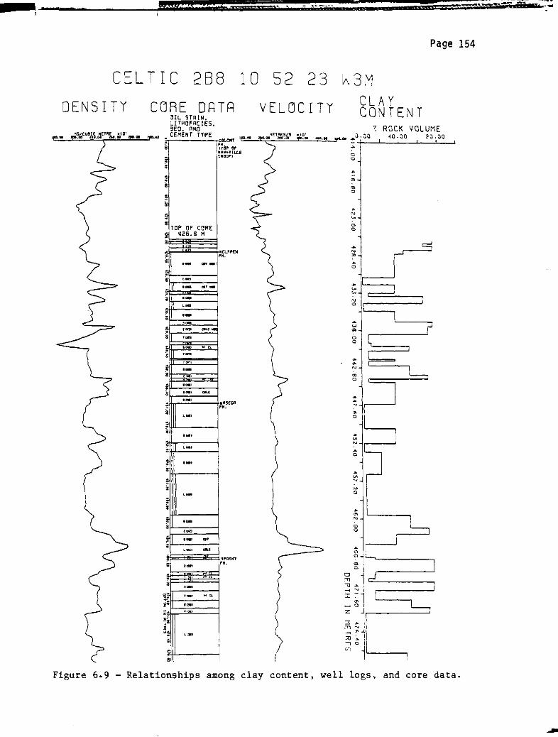
.
Vi'-
S' ......
CELTIC
DENSITY
16pI ili :41, $';
288 1 0 52 23
m:'; ii 55
Page 154
W3M
CLAYCONTENT
:: ROCK VOLUME
'==-..:z::�....::=:__:;.;"�'�=�:__'="=:'.•=-J"". .....0 . :l 0 40 . 00 a a . 00
o
o
1; II
"
�
�:
:if
� ....
S
�.- ..'
aa.C
!PARKT
: ..,.,
F" •
TIn, ",el-
is
��
i; .... ,
z·
s�
i:",.
c.".,
::
!
VELOCITY
OIl
OIl
o
...
N
U
'"
o
...
'"
'"
...
o
,"",
o
...
.....
'"
o
o
...
...
'"
'"
o
...
�-lr---..J'"
o
'"
Q
o
o
...
;;
:
1'-------,"1) ...
..... ""
:!: -:
;s
� ...----------'�
�1...,
'"
;0 ;.
�0
1 '-----,
Figure 6.9 -
Relationships among clay content, well logs, and core data.

'hi*" %iiii; ; .i
===::::.,
�-
-; 1�_
3
Page 155
are unexceptional. The amount of clay content is not directly included
in any of the theoretical models for elastic wave-propagation, but its
effect would be indirectly felt through its influence on other
parameters in the formulae.
Velocity, and to a lesser extent density, are strongly dependent on
saturation conditions. Saturation conditions include the type of pore
fluid (for example, water, brine, gas, or oil) and the degree of
saturation (that is, complete or partial saturation). Numerous
laboratory and theoretical studies of saturation effects have been made.
All of the theoretical models for elastic wave-propagation include
parameters that are directly or indirectly affected by the pore fluid.
Saturation effects have been studied with respect to porosity, pore.
shape, pressure, and the distribution of the fluids within the pore
spaces. General conclusions of this work and their applications to the
present study are as follows:
1. The vel oci ty di fference between fl ui d and gas saturated rocks is
distinguishable only at shallow depths, that is, low differential
pressures (Wyll ie et.!l., 1958; Geertsma, 1961; Gardner et �., 1974;
Toksoz et .!l., 1976). Toksoz et al , (1976) estimated that at
differential pressures corresponding to depths of greater that 2500 m,
in normally-pressured zones, the gas effect will not be visible. Due to
the shallow depth of the Mannville rocks in the study area, the gas
effect should be readily visible.
2. A small quantity of gas (about 5 per cent) in a water saturated rock
reduces the rock velocity significantly, especially at lower
differential-pressure, as are present in the study area. On the other
hand, the presence of oil in water-filled pores has a much less
pronounced effect, and oil content is more linearly related to velocity

..- %4 h';.1£:1 " ; , : ,. """"'''IoU'
-=
d it3
Page 156
(Domenico, 1974, 1976, 1977). The effect of gas saturation should be
much stronger than that of oil saturation in the study area.
3. The compressional-wave velocity in a rock with pore fluid that is
about 5 per cent gas in brine could be lower than the velocity in a pure
gas-saturated rock (Toksoz et !l., 1976). This means that the amount of
gas in the Colony formation will not be linearly related to its effect
on the seismogram.
4. Velocity has little diagnostic value in differentiating between oil
and water reservoirs, and the prospect for identifying the gravity of
crude oil from velocity data is very poor (Gregory, 1976). This means
that the low velocity noticed in the W6 and W3 oil saturated sands is
more likely due to their high porosities than their high oil contents.
In Figure 6.10, lithofacies beds with a high percentage of oil
saturation show a generally lower velocity and density. Both Gregory
(1976) and Domenico (1974) predicted that the effect of oil versus water
saturation would cause only slightly decreased rock velocities. Because
oil saturated zones are also of high porosity, part of the low velocity
effect in the oil zones must be due to their high porosity.
The Colony gas zone has a 10\'1 velocity, as woul d be expected for
even small amount of gas saturation. Density values through this zone
are affected to a relatively lesser degree than are the velocity values,
suggesting that the gas concentration is small.
6.4 Possible Correlation to Real Seismic-Data
Synthetic seismograms have been used since the late 1950s because
they provide a good fit to seismic traces in most cases. Synthetic
seismograms allow geologic insight to the seismic section, and without
this type of control, the significance of the subtle waveform changes

& 1*
CELTIC 288 10 52 23
DENSITY CORE DRTA VELOCITYIHL STRIN.
LITHOFRCIES.BED. RND
CEMENT TlPE
GAS ZONE
ii:
!
ir
�TOP OF CORE
�1126.6 M
�!I
,am
., e,
, ...,
. . ...
=1,-.....:.;:..
:;,.'-::""':;.'--\
���.j.;I,......;I=----+�:�ECR,-
::
... ,
�&IW------t
, ...
�
�I+!.------\
...,
,-
�a1.1------1
....
�Il--.-..
-'-'"-'--I
.,."
�:;I.i------ji� 1IC!i1
j.L.......:•
.:::..,:;,.,----\
5U£
Page 157
W3M
OIL
SATURATION
..
i\)
u
(]I
o
..
(I>
N
...
o
'"
o
Figure 6.10 -
Relationships among oil-saturation values, presence of
gas, well logs, and core data.

%" gr: ;;mil,,
_.
---r--.- --
,..,..." z-- a
Page 158
important to stratigraphic seismic mapping cannot be evaluated. In this
study, synthetic seismograms were used to verify that thin beds within
the Mannville can be mapped. They were also used to analyse the effect
of replacing the coal beds, oil-saturated sand-beds, and gas zone with
brine-saturated, shaley beds If real seismic-data were available in the
study area, the synthetic seismograms would provide a link between the
geology and the seismic section. In addition, the synthetic seismograms
have demonstrated that frequencies in the 60 to 115 hz range will
provide the strongest reflections from the thin, oil-saturated sand-beds
in the Waseca formation. Data acquisition and processing techniques can
now be directed toward improving the amplitudes of the frequencies in
this range. Techniques for high-resolution seismic-recording are
discussed by Farr (1976), Ziolkowski and Lerwill (1979), and Denham
( 1981) •
There can be many differences between synthetic and real
seismic-data, but if care is taken in selecting the synthetic-seismogram
algorithm, in choosing and correcting the data used to construct the
synthetic seismogram, and in processing the real seismic-section, many
of these differences lose their significance. Assumptions made in the
synthetic-seismogram algorithm and the importance of these assumptions
to the present study were discussed in chapter three. In chapter four,
the collection and preparation of the data used to construct the
synthetic seismogram was examined. No real seismic-data was available
in the study area, therefore, the substantial subject of processing the
seismic data to more closely resemble the synthetic data was not
considered.
Many of the differences between synthetic and real seismic-data
stem from the inherent differences in what seismic traces and well logs

e
.. !'d."'hd 41; iT•
•
.......
Page 159
measure. Sheriff (1977) and Ausburn et!l. (1978) studied these
differences and the steps that may be taken to reduce their effects.
However, one of the differences between well-log and seismic data can be
turned to the advantage of this study. Well logs measure rock
properties in a limited zone surrounding the borehole, and so, the
invasion of mud filtrate will usually reduce the effect of hydrocarbons
on well-log measurements (Ausburn, 1977). Seismic waves, however, are
reflected from large areas called Fresnel zones. Synthetic seismograms
are constructed from well logs and, therefore, the hydrocarbon effects
seen on seismograms are minimum effects. In other words, the response
to hydrocarbons could be more prominent on real seismic-traces than on
synthetic seismic-traces. In the present study, this would mean that
the gas, W6, and W3 peaks resulting from the presence of hydrocarbons
(Figure 5.4) could be more pronounced on real seismic-data, if the
deleterious effects of factors such as noise are not severe.

..
--r--
sa
3t_
Page 160
CHAPTER SEVEN
CONCLUSION
The seismic-reflection method is potentially useful to map zones of
economic interest in the Celtic field, if sufficiently high frequencies
can be returned from the Mannville section. Based on studies of
synthetic seismograms, these frequencies are in the range of 60 to 115
hz. But, the natural filtering of the earth forces a dominant frequency
of 40 hz on the Mannville section of the majority of wells studied. In
the synthetic-seismic data, a signal with the 40 hz predominant
frequency had enough high-frequency content to detect the zones of
interest. However, this synthetic data is noise-free; in real-seismic
records, noise may mask the low-amplitude, high-frequency content.
Before seismic programs are started, techniques of data acquisition and
processing must be chosen to accentuate frequencies in the desired
range.
There is a simple one-to-one relationship between the zones of
economic interest and their theoretical seismic response. Subtle
s ratigraphi c changes, or even changes in the saturati ng fl ui ds in the
strata can be directly detected if sufficiently high frequencies and low
noise levels are present.
Mannville geology is extremely variable. The specific results of
this thesis will not likely be applicable in other heavy-oil fields, but
the method used in this study could certainly be applied to other
heavy-oil areas, and even to coal or mineral exploration and
development.

£ '¥hM' ;;:1i ", i
h"
Page 161
REFERENCES
American Petroleum Institute, 1960, API recommended practice for
core-analysis procedure: Washington, American Petroleum
Institute.
Anstey, N.A., 1966, Wiggles: Tulsa, Seismograph Service Corporation.
------- 1977, Seismic interpretation: the physical aspects:
Boston, International Human Resources Development Corporation.
Ausburn, B.E., 1977, Well log editing in support of detailed seismic
studies: Presented at the SPWLA eighteenth Annual Logging
Symposium.
Ausburn, B.E., Nath, A.K., and Wittick, T.R., 1978, Modern seismic
methods--An aid for the petroleum engineer: J. of Petroleum
Technology, v. 20, p. 1519-1529.
Bath, M., 1974, Spectral analysis in geophysics: Amsterdam, Elsevier
Scientific Publishing Co.
Biot, M.A., 1956a, Theory of propagation of elastic waves in a fluid
saturated porous solid; I: Low frequency range: J. of the
Acoustical Soc. of America, v. 28, p. 168-178.
------- 1956b, Theory of propagation of elastic waves in a fluid
saturated porous solid; II: Higher frequency range: J. of the
Acoustical Soc. of America, v. 28, p. 179-191.
Blatt, H., Middleton, G., and Murray, R., 1972, Origin of Sedimentary
Rocks: Englewood Cliffs, Prentice-Hall.
Brandt, H., 1955, A study of the speed of sound in porous granular
media: J. of Applied Mechanics, v. 22. p. 479-486.
Burke, K.B.S., 1968, A seismic study of the surficial deposits in the
Stenen area, Saskatchewan: Geol. Survey of Canada, Paper 68-60.

tt d ==\1'1=+7::i
1 � ....
Page 162
Christiansen, E.A. (editor), 1970, Physical environment of Saskatoon,
Canada: National Research Council of Canada publication
number 11378.
Christopher, J.E., 1974, The Upper Jurassic Vanguard and Lower
Cretaceous Mannville Groups of south-western Saskatchewan:
Sask. Dept. of Mineral Resources Report 151.
------- 1980, The Lower Cretacous Mannville Group of
Saskatchewan--A tectonic overview: Sask. Geol. Soc.
Special Publ. No.5, p. 3-32.
Christopher, J.E., Kent, D.M., and Simpson, F., 1971 Hydrocarbon
potential of Saskatchewan: Sask. Dept. of Mineral Resources
Report 157.
Crain, E.R., and Boyd, J.D., 1979, Determination of seismic response
using edited well log data: Presented at the Seventh Formation
Evaluation Symposium of the Canadian Well Logging Soc.
Denham, L.R., 1981, Extending the resolution of seismic reflection
exploration: J. of the Canadian Soc. of Exploration Geophysicists,
v. 17, p. 43-54.
Domenico, S.N., 1974, Effect of water saturation on seismic reflectivity
of sand reservoirs encased in shale: Geophysics, v. 39,
p. 759-769.
------- 1976, Effect of brine-gas mixture on velocity in an
unconsolidated sand reservoir: Geophysics, v. 41, p. 882-894.
------- 1977, Elastic properties of unconsolidated porous sand
reservoirs: GeophysiCS, v. 42, p. 1339-1368.
Dunning, N.E., Henley, H.J., and Lange, A.G., 1980, The Freemont field:
An exploration model for the Lloydminster area: Sask. Geol.
Soc. SpeCial Publ. No.5, p. 132-148.

3
Page 163
Farr J.B., 1976, How high is high resolution?: Presented at the 46th
Annual Meeting of the Soc. of Exploration Geophysicists.
Focht, G.W., and Baker, F.E., 1979, Geophysical Case History of the Two
Hills Colony gas field of Alberta: Presented at the 49th Annual
Meeting of the Soc. of Exploration Geophysicists.
Fuglem, M.O., 1970, Use of core in evaluation of productive sands,
Lloydminster area; in: Bundle, J.E. and Holmberg, R.A. (editors),
Saskatchewan Mesozoic core seminar, Sask. Geol. Soc.
Futterman, W.I., 1962, Dispersive body waves: J. of Geophysical
Research, v. 67, p. 5279-5291.
Ganley, D.C., 1979, The measurement of Q from seismic data: Ph.D.
thesis, University of Alberta, Edmonton, unpublished.
------- 1981, A method for calculating synthetic seismograms which
include the effects of absorption and dispersion: Geophysics, v.
46, p. 1100-1107.
Gardner, G.H.F., Gardner, L.W., and Gregory, A.R., 1974, Formation
vel oci ty and dens; ty--The di agnosti c basi cs for strati graphi c
traps: Geophysics, v. 39, p. 770-780.
Gary, M., McAfee, R.Jr., and Wolf, C.L., 1974, Glossary of Geology:
Washington, American Geological Institute.
Gassman, F., 1951, Elastic waves through a packing of spheres:
Geophysics, v. 16, p. 673-685.
Gendzwil1, D.J., 1982, Personal Communication, Dept. of Geological
Sciences, U. of Saskatchewan, Saskatoon.
Geertsma, J., 1961, Velocity log interpretation: The effect of rock
bulk compressibility: Soc. of Petroleum Engineers Journal, v. 1,
p. 235-248.
---

'M "§Ph,,$I. i , •
: =:::r='-:. 7£ '�£
Page 164
Greensmith, J.T., 1978, Petrology of the sedimentary rocks: Great
Britian, George Allen and Unwin Ltd.
Gregory, A.R., 1976, Fluid saturation effects on dynamic elastic
properties of sedimentary rocks: Geophysics, v. 41, p. 895-921.
------- 1977, Aspects of rock physics from laboratory and log
data that are important to seismic interpreptation: American
Association of Petroleum Geologists Memoir 26, p. 15-46.
Gross, A.A., 1980, Mannville channels in east-central Alberta:
Sask. Geo1. Soc. Special Pub1. No.5, p. 33-63.
Haid1, F., 1980, Correlation of lithofacies and lithostratigraphic units
in the Mannville Group, Lloydminster area, Saskatchewan: Sask.
Geo1. Soc. Special Pub1. No.5, p. 218-235.
-----�- 1981, Personal Communication, Serendipity Geological
Consultants Ltd., Regina, Sask.
Hajnal, Z., 1982, Personal Communication, Dept. of Geological Sciences,
U. of Saskatchewan, Saskatoon.
Hamilton, E.L., 1972, Compressional-wave attenuation in marine
sediments: Geophysics, v. 37, p. 620-646.
Hauge, P.S., 1981, Measurements of attenuation from vertical seismic
profiles: Geophysics, v. 46, p. 1548-1558.
Jenkins, F.A., and White, H.E., 1957, Fundamentals of optics: New York,
McGraw-Hill Book Company, Inc.
Johnston, D.H., Toksoz, M.N., and Timur, A., 1979, Attenuation of
seismic waves in dry and saturated rocks: II. Mechanisms:
Geophysics, v. 44, p. 691-711.
Johnson, D.H., and Toksoz, M.N., 1981, Definitions and
terminology; in: Seismic wave attenuation, Soc. of Exploration
Geophysicists reprint series No.2, p. 1-5.
111m2' d i :1,4 i;= a.
, ....
3
Page 165
Kallweit, R.S., and Wood, L.C., 1982, The limits of resolution of zero-
phase wavelets: Geophysics, v. 47, p.1035-1046.
Karr, C.Jr., 1978, Analytical methods for coal and coal products,
volume 1: New York, Academic Press.
King, M.S., 1966, Wave velocities in rocks as a function of changes in
over-burden pressure and pore fluids: Geophysics, v. 31, p. 50-73.
Koefoed, 0., 1981, Aspects of vertical seismic resolution: Geophysical
Prospecting, v. 29, p. 21-30.
Kuster, G.T., and Toksoz, M.N., 1974, Velocity and attenuation of
seismic waves in two-phase media: Part I. Theoretical
formulations: Geophysics, v. 39, p.587-606.
Lorsong, J.A., 1979, Lithofacies of the Lower Cretaceous Mannville
Group, west-central Saskatchewan: Sask. Dept. of Mineral Resources
Misc. Report 80-4, p. 109-111.
------- 1980, Geometry of nearshore sand bodies in the Upper
Mannville Group, Celtic field, Saskatchewan: Sask. Geol. Soc.
Special Publ. No.5, p. 236-266.
------- 1981, Diagenesis and heavy oil emplacement in Upper
Mannville reservoirs, Celtic field, west-central Saskatchewan:
Sask. Dept. of Mineral Resources Misc. Report 81-4, p. 141-148.
------- 1981, Personal Communication, Serendipity Geological Consultants
Ltd., Regi na, Sask.
------- 1982, Personal Communication, Serendipity Geological Consultants
Ltd., Regina, Sask.
Meckel, L.D.Jr., and Nath, A.K., 1977, Geological considerations for
stratigraphic modeling and interpretations: American Association of
Petroleum Geologists Memoir 26, p. 417-438.

fnw@' 01: i i 5 m:='"_-
a-f
-wIIIII
Page 166
Morlet, J., Arens, G., Fourgeau, E., and Giard, D., 1982, Wave
propagation and sampling theory--Part 1: Complex signal and
scattering in multilayered media: Geophysics, v. 47, p. 203-221.
Nafe, J.E., and Drake, C.L., 1963, Physical properties of marine
sediments; in: Hill, M.N. (editor), The earth beneath the sea-
History: New York, Interscience publishers, p.794-815.
Neidell, N.S. and Poggiagliolmi, E., 1977, Stratigraphic modeling and
interpretation--Geophysical principles and techniques: American
Association of Petroleum Geologists Memoir 26, p. 389-416.
North, B.R., and Caldwell, W.G.E., 1975, Foraminiferal faunas in the
Cretaceous system of Saskatchewan: Geol. Association of Canada
Special Paper No. 13, p. 303-331.
Patterson, A.R., 1964, Datum corrections in glacial drift: Geophysics,
v. 29, D. 957 -967 •
Pettijohn, F.T., 1975, Sedimentary rocks, third edition: New York, F.T.
Petti john.
Peterson, R.A., Fillippone, W.R., and Coker, F.B., 1955, The synthesis
of seismograms from well log data: Geophysics, v. 20, p. 516-538.
O'Connell, R.J., and Budiansky, B., 1974, Seismic velocities in dry and
saturated cracked solids: J. of Geophysical Research, v. 79, p.
5412-5426.
O'Doherty, R.F., and Anstey, N.A., 1971, Reflections on amplitudes:
Geophysical prospecting, v. 19, p. 430-458.
Orr, R.D., Johnston, J.R., and Manko, E.M., 1977, Lower Cretaceous
geology and heavy-oil potential of the Lloydminster area: Bull. of
Canadian Petroleum Geology, v. 25, p. 1187-1221.

* ItH
w. ===
..
'0........- at,
--
5
Page 167
Putman, P.E., 1980, Fluvial deposition within the Upper Mannville of
west-central Saskatchewan: Stratigraphic implications: Sask. Geol.
Soc. Special Publ. No.5, p. 197-216.
Reilkoff, B.R., 1982, Processing reflection seismic data from the
Athabasca Basin: M.Sc. thesis, University of Saskatchewan,
Saskatoon, unpublished.
Ricker, N., 1953a, The form and laws of propagation of seismic wavelets:
Geophysics, v. 18, p. 10-40.
------- 1953b, Wavelet contraction, wavelet expansion and the control of
seismic resolution: Geophysics, v. 18, p. 769-792.
Robinson, E.A., and Treitel, S., 1977, The spectral function of a
layered system and the determination of the waveform at depth:
Geophysical Prospecting, v. 25, p. 434-459.
Ruter, H., and Schepers, R., 1978, Investigation of the seismic response
of cyclically layered carboniferous rock by means of synthetic
seismograms: Geophysical Prospecting, v. 26, p. 29-47.
Sask. Dept. of Mineral Resources, 1979, Reservoir annual 1978: Sask.
Dept. of Mineral Resources Misc. Report 79-8.
Sask. Dept. of Mineral Resources, 1983, Personal Communication, Geology
and Mines Geodata Division, Regina.
Schoenberger, M., 1974, Resolution comparison of minimum-phase and zero-
phase signals: Geophysics, v. 39, p. 826-833.
Schoenberger, M., and Levin, F.K., 1974, Apparent attenuation due to
intrabed multiples: Geophysics, v. 39, p. 278-291.
------- 1978, Apparent attenuation due to intrabed multiples, II:
Geophysics, v. 43, p. 730-737.
Schriener, B., 1981, Personal Communication, Sask. Research Council,
Saskatoon.
3 'd.4iii?' "$: 'it' f
i
=. =.;o=�
_,t
!f ........
Page 168
Sengbush, R.L., Lawrence, P.L., and McDonal, F.J., 1961, Interpretation
of synthetic seismograms: Geophysics, v. 26, p138-157.
Sereda, I.T., 1978, A crustal reflection expanding-spread study in
southeast Saskatchewan and southwest Manitoba: M.Sc. thesis,
University of Saskatchewan, Saskatoon, unpublished.
Sheriff, R.E., 1973, Encyclopedic dictionary of exploration geophysics:
Tulsa, Society of Explortion Geophysicists.
------- 1977, Limitations on resolution of seismic reflections and
geologic detail derivable from them: American Association of
Petroleum Geologists Memoir 26, p. 3-14.
Simpson, F., 1975, Marine lithofacies and biofacies of the Colorado
Group (Middle Albian to Santonian) in Saskatchewan: Geol.
Association of Canada Special Paper No. 13, p. 553-587.
Simpson, F., 1981, Low-permeability gas reservoirs in marine
Cretaceous sandstones of Saskatchewan: 13. Upper Colorado
(Turonian to Santonian) strata of west-central Saskatchewan:
Sask. Dept. of Mineral Resources Misc. Report 81-4, p. 159-162.
Stone, D.G., 1980, Statistical relations between borehole and surface
data: Presented at the 50th Annual Meeting of the Society of
Exploration Geophysicists.
Titchkosky, K.A., 1968, Seismic deconvolution, volume II: Calgary,
Evelyn DeMille Books Ltd.
Toksoz, M.N., Cheng, C.H., and Timur, A., 1976, Velocities of seismic
waves in porous rocks: Geophysics, v. 41, p. 621-645.
Toksoz, M.N., and Johnston, D.H. (editors), 1981, Field measurements of
attenuation; in: Seismic wave attenuation, Soc. of Exploration
Geophysicists Geophysics reprint series No.2, p. 250-251.

s \*. t *=*0'" f.41§P@;
" '"i. --�.-
'--r-. =;--7"-
PflIoe 169
Vigrass, L.W., 1965, General geology of heavy oil accumulations in
western Canada (including the Athabasca tar sands): The J. of
Canadian Petroleum Technology, v. 4, p. 87-94.
Vigrass, L.W., 1977, Trapping of oil at intra-Mannville (Lower
Cretaceous) disconformity in Lloydminster area, Alberta and
Saskatchewan: The American Association of Petroleum Geologists
Bull., v. 61, p. 1010-1028.
de Voogd, N., and den Rooijen, H., 1983, Thin layer response and
spectral bandwidth: Geophysics, v.48, p. 12-18.
Walsh, J.B., and Grosenbaugh, M.A., 1979, A new model for analyzing the
effect of fractures on compressibility: J. of Geophysical Research,
v. 84, p.3532-3536.
Wennekers, J.H.N., Ryckborst, H., Abougoush, M.S., McCreary, R.K.V., and
Letkeman, J.P., 1979, Heavy oil, tar sands play key role in
Alberta, Saskatchewan production, Part 1: Oil and Gas J., v. 77,
p. 290-304.
White, W.I., and von Osinski, W.O., 1977, Geology and heavy oil reserves
of the Mannville Group, Lloydminster-North Battleford area,
Saskatchewan: Sask. Dept. of Mineral Resources, Petroleum and
Natural Gas Branch.
Widess, M.B., 1973, How thin is a thin bed: Geophysics, v. 38,
D. 1176-1180.
Widess, M.B., 1982, Quantifying resolving power of seismic systems:
Geophysics, v. 47, p. 1160-1173.
Williams, G.D., 1963, The Mannville Group (Lower Cretaceous) of central
Alberta: Bull. of Canadian Petroleum Geology, v. 11, p. 350-368.
--

.S....'I�t__���t Jji§l�=iil§;=j;=S=;:,,=!;==�;;:;:,��::::�::!.�-:.:t��:::::::=::;====ism=����==���-�-;;_d__
Page 170
Wyllie, M.R.J., Gregory, A.R., and Gardner, L.W., 1956, Elastic wave
velocities in heterogeneous and porous media: Geophysics, v. 21, p.
41-70.
Wyllie, M.R.J., Gregory, A.R., and Gardner, G.H.F., 1958, An
experimental investigation of factors affecting elastic wave
velocities in porous media: Geophysics, v. 23, p. 459-493.
Ziolkowski, A., and Lerwill, W.E., 1979, A simple approach to high
resolution seismic profiling for coal: Geophysical Prospecting,
v. 27, p. 360-393.

& .. mlh'3:iI Oit':ij:; j
Page 171
APPENDIX A
Core-analysis data, as stored in the CA.DAT files
--

twa ,>*"
fi t:g:; :,-
....... - ...
_-).-_- === -z; -
tt be"
i
Page 172
CA4B2.DAT
01 B WB .3 452.1 4 .26 .10 257. 35.
02 L WI .3 451.8 3 .19 • 03 10 • 3.
03 B WB 2.8 449.0 a .27 • 28 260 • 35.
04 L W3 5.4 443.6 a .35 .72 1037. 3.
05 B WB 2.6 441.0 0 .30 • 46 400 • 35.
06 L W4 1.0 440.0 0 .35 .56 2920. 3.
07 B WB 1.5 438.5 0 .27 .28 260. 35.
08 L W6 4.5 434.0 0 .33 .74 6115. 2.
09 B MB .8 433.2 1 .19 . 03 10 • 60.
10 B MB .2 433.0 6 .19 • 03 10 • 40.
11 B MB .1 432.9 3 .19 • 03 10 • 40.
CA2D2.DAT
01 L 52 2.2 467.1 a .29 .72 1540. 2.
02 Z 5Z .1 467.0 a .22 • 07 10 • 55.
03 L 52 2.6 464.4 0 .35 • 77 1540 • 2.
04 Z 5Z .8 463.6 a .22 • 07 10 • 55.
as B 5B 1.4 462.2 a .28 .43 260. 35.
06 T 53 1.6 460.6 2 .27 .31 500. 12.
07 L S3 1.1 459.5 2 .28 .46 890. 4.
08 Z 5Z .5 459.0 0 .22 .07 10. 65.
09 B SB • 8 458.2 a .30 .47 500. 20 •
10 Z SZ 4.4 453.8 8 .21 • 07 8 • 50.
11 B WB 2.3 451.5 a .27 .31 300. 30.
12 L W3 .8 450.7 a .36 .69 1540. 3.
13 B WB .3 450.4 0 .28 • 43 400 • 30.
14 L W3 4.1 446.3 0 .35 .70 1540. 2.
15 B WB 2.6 443.7 a .33 .67 600. 20.
16 L W4 .9 442.8 a .33 .66 1540. 3.
17 B WB 1.6 441.2 a .28 .43 400. 35.
18 L W6 4.2 437.0 a .39 .80 1540. 2.
19 B MB 3.6 433.4 2 .29 .48 260. 35.
20 T M2 2.9 430.5 2 .33 .60 350. 12.
21 C MC .5 430.0 0 .06 .01 1. 1-
22 L M4 .8 429.2 a • 35 .67 600 • 3.
23 Z MZ 1.8 427.4 4 .22 .07 10. 70.
24 5 M5 1.6 425.8 0 .23 .05 2. 75.
25 B MB 1.4 424.4 2 • 28 .43 260 . 35.
26 T MT .5 423.9 a • 28 .56 420 • 5.
27 C MC .2 423.7 a .26 .07 10. 35.
28 5 M5 .6 423.1 a • 23 .05 2 . 75.
29 B MB .5 422.6 a .32 .67 546. 20.
30 T M5 2.5 420.1 a .29 .45 420. 13.
31 5 CS .4 419.7 a .23 .05 2. 75.
32 T C1 .7 419.0 a .31 .51 570. 5.
33 Z CZ 1.2 417.8 a .22 .07 10. 70.
34 T C1 .4 417.4 0 .32 .51 570. 5.
35 5 C5 .4 417.0 a .22 .07 10. 75.
36 T CT 4.1 412.9 2 .31 .40 570. 5.
37 5 CS .3 412.6 a • 22 .07 10 • 75.

"hi' iN 't' ,[2 : # :=rm ET�7 t
,j!J..
Page 173
38 M CM 1.2 411.4 1 .21 .07
39 S CS .2 411.2 0 .22 .07
40 T CT 3.2 408.0 1 .21 .07
228. 14.
10. 75.
228. 14.
CA4D2.DAT
01 B RB 2.4 488.4 0 .27 • 51 400 • 35.
02 S GS 1.7 486.7 0 .23 • 05 2 . 75.
03 L G1 5.1 481.6 0 .35 • 72 1585 • 2.
04 B GB .2 481.4 0 .27 • 20 260 • 50.
05 L G1 .4 481.0 3 .14 .68 24. 3.
06 L G1 1.2 479.8 0 .32 • 66 1088 • 3.
07 T G1 1.8 478.0 1 .29 • 38 80 • 13.
08 S SS .3 477.7 0 .23 .05 2. 75.
09 B S8 3.9 473.8 0 .29 • 34 400 • 35.
10 T S2 1.1 472.7 0 .34 .71 2388. 5.
11 B SB .3 472.4 0 .24 • 41 100 . 65.
12 L S2 3.8 468.6 0 .35 .71 764. 3.
13 S SS .3 468.3 0 .23 .05 2. 75.
14 Z SZ .4 467.9 0 .22 .07 10. 70.
15 B S8 .9 467.0 0 .28 • 39 500 • 35.
16 L S3 1.5 465.5 2 .28 • 40 44 • 12.
17 S SS .4 465.1 0 .23 .05 2. 75.
18 Z SZ .3 464.8 0 .22 .07 10. 70.
19 S SS .7 464.1 0 .23 .05 2. 75.
20 T S5 .3 463.8 0 .33 .40 1200. 5.
21 S SS .3 463.5 0 .23 • 05 2 • 75.
22 M S5 .5 463.0 2 .27 • 26 55 • 12.
23 S SS 1.3 461.7 8 .22 .05 2. 75.
24 Z SZ .8 460.9 8 .21 • 07 8 • 65.
25 T W1 2.8 458.1 9 .21 .22 100. 10.
26 B WB 2.3 455.8 0 .27 .33 300. 35.
27 L W3 4.8 451.0 0 .35 • 74 770 • 2.
28 8 WB 2.3 448.7 0 . 31 • 64 600 . 20 •
29 L W4 1.6 447.1 0 • 33 .72 1432. 2 •
30 B WB 1.8 445.3 0 • 28 . 49 500 • 30 •
31 L W6 3.9 441.4 0 • 35 . 79 3199 • 2 •

§41p' I' 'm... 4( .......
-
1tiII .......
&_..... . - ..
--;------ ..... .
j
Page 174
CA2B8.DAT
01 B RB 1.1 492.9 0 .30 • 39 400 • 35.02 Z GZ .2 492.7 0 .22 • 07 10 • 70.
03 5 GS 1.9 490.8 0 .23 .05 2. 75.
04 L G1 4.5 486.3 0 .34 • 71 1493 • 2.
05 T G1 .4 485.9 0 .36 • 51 400 • 5.
06 M G1 .5 485.4 0 .32 .57 501. 7.
07 T G1 .7 484.7 3 .14 • 03 30. 5 •
08 T G1 1.7 483.0 2 .27 • 30 350 • 12.
09 5 55 .5 482.5 0 .23 .05 2. 75.
10 B 5B 3.4 479.1 0 .28 .35 300. 45.
11 L 52 5.1 474.0 0 .33 • 66 434 • 2.
12 Z SZ .7 473.3 0 .22 .07 10. 70.
13 B 5B 1.0 472.3 0 .26 • 31 260. 50 •
14 T 53 1.2 471.1 2 .25 • 31 350 • 12.
15 5 55 1.1 470.0 0 .23 .05 2. 75.
16 C 5C .4 469.6 0 .06 .01 1- 5.
17 T 55 .5 469.1 2 .23 .36 350. 12.
18 M 55 .4 468.7 2 .25 • 28 228 • 13.
19 Z 5Z 1.6 467.1 0 .22 • 07 10 • 75.
20 T WT .2 466.9 2 .23 .34 350. 12.
21 L WI .4 466.5 6 .14 • 03 30 • 2.
22 L WI 1.3 465.2 3 .14 • 03 30 • 2.
23 B WB 1.3 463.9 6 .19 • 25 10 • 35.
24 Z WI .8 463.1 0 .22 • 07 10 • 70.
25 B WB 1.6 461.5 0 .27 • 25 260 • 50.
26 L W3 5.2 456.3 0 .35 • 70 713 • 4.
27 B WB 2.8 453.5 0 .30 • 63 600 • 20.
28 L W4 1.1 452.4 0 .32 • 73 1540 . 2.
29 B WB 1.9 450.5 0 • 31 • 28 400 • 35 •
30 L W6 3.1 447.4 0 .36 • 83 4710 • 2.
31 B MB .9 446.5 0 • 32 .40 400 • 35.
32 B MB 1.0 445.5 3 .19 • 03 10 • 35.
33 B MB .9 444.6 0 • 32 • 30 400 . 35 •
34 M MM .4 444.2 7 • 27 • 49 500 • 7 •
35 Z MZ .5 443.7 0 .19 • 47 10 • 70.
36 B MB 1.2 442.5 0 .29 • 23 260 • 50.
37 T MT .6 441.9 0 .34 • 58 420 • 7.
38 B MB .2 441.7 0 • 32 .48 400 • 35.
39 T MT 1.1 440.6 0 .31 • 53 93 • 7.
40 B MB .6 440.0 2 • 27 .27 260 • 50.
41 C MC .4 439.6 0 .06 .01 1- 10.
42 T MT 1.1 438.5 0 .37 .49 420. 7.
43 Z MZ 1.0 437.5 5 .22 .07 10. 70.
44 5 M5 .6 436.9 0 .23 • 05 2 • 75.
45 B MB 1.4 435.5 0 .27 .36 1210. 35.
46 L M5 1.0 434.5 0 .31 .66 2180. 2.
47 B MB .9 433.6 0 .23 .41 100. 65.
48 M r1-1 .4 433.2 0 .38 .48 280. 7.
49 B MB 1.1 432.1 8 .17 .50 257. 35.
50 C Me .9 431.2 0 .06 .01 1. 1.
51 B MB 3.0 428.2 8 .31 .43 257. 35.
52 e ee • 5 427.7 0 .26 .07 10. 45 •
53 5 e5 .5 427.2 0 .23 • 07 2 • 75.

&
Page 175
54 B CB .3 426.9 0 .23 .41 100. 65.
555 C5 .3426.60.23.05 2.75.
CA4B8.DAT
01 M R1 .5 513.1 1 • 24 • 07 220 • 13 •
02 M R1 .7 512.4 3 • 14 • 03 30 • 7 •
03 M R1 .2 512.2 1 .24 . 07 220 • 13.
04 Z RZ .4 511.8 0 • 22 .07 10 • 70.
05 5 R5 1.6 510.2 0 .23 • 05 2. 75 •
06 Z RZ 2.0 508.2 0 .22 • 07 10 • 70.
07 B RB 1.7 506.5 6 • 26 • 22 257 • 35 •
08 Z GZ 1.2 505.3 0 • 22 • 07 10 • 70 •
09 L G1 5.6 499.7 0 .34 • 64 1447. 2 •
10 B GB .5 499.2 7 • 24 • 41 100 • 65 •
11 L G1 .7 498.5 0 • 31 • 48 1227 • 3 •
12 T G1 .9 497.6 2 • 26 • 28 350 • 13 •
13 M G1 .3 497.3 2 • 27 • 31 200 • 12 •
14 T G1 1.1 496.2 2 • 30 • 37 400 • 7 •
15 5 55 1.1 495.1 0 .23 • 05 2. 75 •
16 B 5B 3.4 491.7 8 .28 • 37 400. 35 •
17 L 52 1.4 490.3 0 .31 • 47 181. 4 •
18 B 5B .3 490.0 0 • 28 .41 400 • 35.
19 L 52 3.1 486.9 0 • 32 • 74 1031 • 2 •
20 5 55 .7 486.2 0 • 23 .05 2. 75 •
21 L 53 2.2 484.0 2 • 24 • 25 500 • 12 •
22 B 5B .7 483.3 2 .28 • 33 350. 40 •
23 C 5C .4 482.9 0 .06 .01 1. 5.
24 Z 5Z .9 482.0 0 • 22 .07 10. 70 •
25 B 55 .7 481.3 8 • 33 .40 450. 35 •
26 T 55 .6 480.7 1 .26 .27 300. 13.
27 Z 5Z 1.7 479.0 9 .22 • 07 10. 70 •
28 T WI 1.2 477.8 7 .25 .30 350. 5.
29 T WI .6 477 .2 3 .13 .03 30. 5.
30 B WB 1.0 476.2 3 .19 .03 10. 35.
31 B WB 1.8 474.4 0 .28 .15 260. 35.
32 L W3 5.1 469.3 0 .35 .67 557. 4.
33 B WB 1.2 468.1 0 • 30 .42 400 • 35.
34 Z WZ .8 467.3 0 .22 .07 10. lD.

II" NV? dl4l,' I' ; : !_-
-;-5,a-.
·--f-- - -_ -
:;m'::''......
j
Page 176
CA2D8.DAT
01 B SB .3 506.7 0 .34 .16 600. 20.02 T S2 .8 505.9 0 .32 .19 545. 5.03 L S2 3.2 502.7 0 .34 .57 700. 4.04 Z SZ .8 501.9 0 .22 .07 10. 70.05 M S3 .6 501.3 0 .26 .26 3l. 7.06 T S3 .6 500.7 0 .26 .29 68. 5.07 M S3 1.4 499.3 3 .14 .03 30. 7.
08 M S3 .6 498.7 2 .28 .32 32. 7.
09 S SS .2 498.5 0 .23 .05 2. 75.
10 L S5 1.2 497.3 2 .29 .39 66. 4.
11 S SS .5 496.8 0 .23 .05 2. 75.
12 L SL .3 496.5 2 .32 .30 66. 12.
13 Z SZ .4 496.1 0 .22 .07 10. 70.
14 M WI .9 495.2 3 .14 .03 30. 7.
15 M WI .6 494.6 2 .26 .30 32. 12.
16 Z WZ 1.7 492.9 0 .22 .07 10. 70.
17 T WT 1.1 491.8 1 .24 .07 30. 5.
18 Z WI .3 491.5 0 .22 .07 10. 70.
19 B WB .8 490.7 0 .30 • 40 400 • .35.
20 L WL .3 490.4 1 .22 .24 30. 13.
21 B WB 1.4 489.0 0 .30 .40 400. 35.
22 L W3 2.0 487.0 0 .33 .56 275. 4.
23 B WB .8 486.2 0 .29 .21 260. 35.
24 S WS .5 485.7 0 .23 .05 2. 75 •
25 L WL .3 485.4 0 • 31 .51 1320. 4.
26 B WB 2.7 482.7 0 .27 .36 546. 30.
27 L W4 .5 482.2 0 .35 .46 1320. 4.
28 B WB • 2 482.0 0 .27 .36 546. 30 .
29 L W4 1.8 480.2 0 .33 .57 1419. 3.
30 B WB 1.7 478.5 0 .37 .43 546. 20.
31 L W6 • 5 478.0 2 • 30 .59 67 • 12 •
32 L W6 3.3 474.7 0 .40 .83 4912. 2.
33 B MB .3 474.4 2 • 23 .23 250. 65 •
34 Z MZ .4 474.0 3 .21 .07 2. 70.
35 B MB 1.2 472.8 2 • 26 .22 257. 50 •
36 L ML .8 472.0 9 • 29 .67 541. 8 •
37 B MB .8 471.2 0 • 23 .41 100. 65 •
38 M MM .2 471.0 0 .26 • 28 731. 7 •
39 B MB .7 470.3 0 .30 • 40 546. 30 •
40 L M2 3.6 466.7 0 .32 • 51 257. 4 •
41 C MC .2 466.5 0 .24 • 07 10. 40 •
42 L M4 .9 465.6 0 .34 .63 606. 3.
43 Z MZ 1.7 463.9 4 .21 • 07 2 • 70.
44 S MS 1.3 462.6 0 .23 • 05 2 • 75.
45 L ML 1.8 460.8 0 .28 • 52 446. 4 •
46 B MB 1.1 459.7 7 .26 .23 257. 35.
47 L ML 2.0 457.7 0 .30 • 37 404. 4 •
48 S MS .5 457.2 0 .23 • 05 2 • 75.
49 B MB .5 456.7 a .27 .36 546. 30.
50 L ML 1.5 455.2 0 .34 .62 1824. 2.
51 C CC .2 455.0 a .24 • 07 10. 40 •
52 7 CZ .8 454.2 a .26 .07 15. 65.
53 S CS .7 453.5 a .23 .05 2. 75.
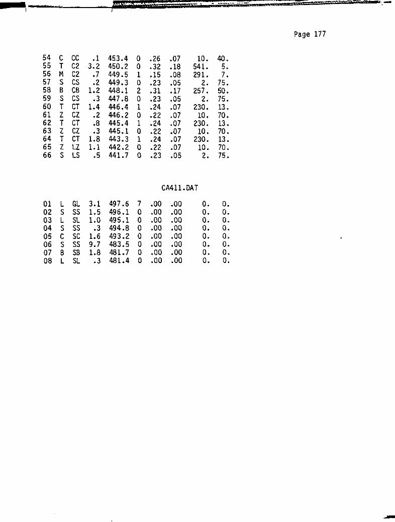
"WaHit.
'H; : :-
....,.......
..-.. 7:
.-- , �
---r-_.
\t
tt t
e- It
0 Z[
i
Page 177
54 C CC .1 453.4 0 • 26 .07 10 • 40.55 T C2 3.2 450.2 0 .32 .18 541. 5.56 M C2 .7 449.5 1 .15 .08 291. 7.57 S CS • 2 449.3 0 .23 .05 2. 75 •
58 B CB 1.2 448.1 2 • 31 .17 257 • 50.
59 S CS • 3 447.8 0 .23 .05 2. 75 •
60 T CT 1.4 446.4 1 • 24 .07 230 • 13.
61 Z CZ • 2 446.2 0 • 22 .07 10 • 70 •
62 T CT • 8 445.4 1 • 24 .07 230 • 13 •
63 Z CZ .3 445.1 0 • 22 .07 10. 70 •
64 T CT 1.8 443.3 1 • 24 .07 230 • 13.
65 Z LZ 1.1 442.2 0 .22 .07 10. 70.
66 S LS .5 441.7 0 .23 .05 2. 75.
CA411.DAT
01 L GL 3.1 497.6 7 .00 .00 o. o.
02 S SS 1.5 496.1 0 .00 .00 o. o.
03 L SL 1.0 495.1 0 .00 • 00 o . O.
04 S SS .3 494.8 0 .00 .00 o. O.
05 C SC 1.6 493.2 0 • 00 .00 o . O.
06 S SS 9.7 483.5 0 .00 .00 O. O.
07 8 S8 1.8 481.7 0 .00 • 00 o. O •
08 L SL .3 481.4 0 .00 .00 o. o.

3 ".iiI;% "7::' ;- .. _ ...
·_-aO....... it '-..-
Page 178
APPENDIX B
Listings of computer programs

'hLlilN'41, i i ,�-
. ..,.. _.
'--r-- :: ;;e
Page 179
C***********************************************************************
C
C CELGRF
C
C***********************************************************************
C
C
C PURPOSE: CELGRF IS USED TO PLOT THE SYNTHETIC SEISt�OGRAM
C PRODUCED BY SYNCEL. CELGRF PLOTS THE SYNTHETIC SEISMOGRAM
C VERSUS TIME AND DEPTH; THE SHAPE AND NORMALIZED AMPLITUDE
C SPECTRUM OF THE RICKER-WAVELET SOURCE (IF IT IS USED);C THE Q, VELOCITY AND DENSITY VALUES FOR THE WELL; THE
C STRATIGRAPHIC MARKERS; AND THE CORE PROPERTIES OF
C POROSITY, PERMEABILITY, OIL SATURATION, CLAY CONTENT,C CEMENT TYPE, AND LITHOFACIES TYPE
C
C
C
C
C PROGRAMMER:
C
C
C
C
C
C
C
C
AS SEVERAL PAGES OF PLOTS ARE PRODUCED,
2-STEP CALCOMP PLOTTING IS SUGGESTED
M.K. LOMAS
DEPT. OF GEOLOGICAL SCIENCES (GEOPHYSICS)
U. OF SASKATCHEWAN
SASKATOON
1982
SCALING FACTORS ARE SPECIFIED IN THE PROGRAM
A FILE CALLED SPECAN.DAT IS WRITTEN TO DISK AND CAN BE
AS INPUT TO THE SPECTRAL ANALYSIS PROGRAM SPECAN.FOR
USED
C***********************************************************************
C
C**********
C DIMENSION SECTION
C**********
REAL*8 DELT,DELTIM,S(8192),PWRINTEGER UNIT(100),CEM(100),PO,LABEL1(S),LBLZ(11),LBL3(11),LBL4(lZ)
*,LBLS(9),LBL6(lZ),LBL7(4),LBL8(8),LBL9(7),LBLIO(11),LBLll(Z),
*LBL12(Z},LBL13(7},LBL14(7),LBL1S(11),LBL16(6)REAL INTIME( 4001) , LCOLO ,r�ANN ,
MONTAN , LEAPK,MCLARNDIMENSION Z(4001),CO(4001),QO(4001),RHO(4001),TT(4001),
.ADEPTH(4001),ATIME(4001) ,AZ(4001),ACO(4001) ,ARHO(4001) ,AQO(4001)DIMENSION XT(819Z),TWTIME(819Z),TDEPTH(4001),SYNDEP(819Z),
.FREQ(lOOOO) ,WAVAMP(lOOOO),SS(lOOOO) ,TTIME(4001),CCO(lOO),RRHO(lOO)DIMENSION FAC(lOO),BED(lOO,Z),THICK(lOO),TOPBED(lOO),
*POR(lOO),OILSAT(lOO),PERM(lOO),CLAY(lOO),WAVE(SOOO),WAVTIM(SOOO)C
C**********
C OPEN STATEMENTS
C**********
OPEN(UNIT=Zl,DEVICE='DSK' ,ACCESS='SEQIN' ,FILE='SYNGAN.DAT',.DIALOG)
OPEN(UNIT=Z2,DEVICE='DSK', ACCESS='SEQIN' ,FILE='GANCEL.DAT',.DIALOG)
OPEN(UNIT=Z3,DEVICE='DSK' ,ACCESS='SEQIN' ,FILE='AU.DAT' ,DIALOG)OPEN(UNIT=Z4,DEVICE='DSK' ,ACCESS='SEQIN' ,FILE='DEN.DAT' ,DIALOG)OPEN(UNIT=Z5,OEVICE='DSK' ,ACCESS='SEQIN' ,FILE='WAVE.OAT' ,DIALOG)

£ MPH'S: '$4 I - � . _.-
--r-.. =:
Page 180
OPEN(UNIT=26,DEVICE='DSK' ,ACCESS='SEQIN' ,FILE='WAVAMP.DAT',.DIALOG)
OPEN(UNIT=28,DEVICE='DSK' ,ACCESS='SEQIN' ,FILE='COQO.DAT' ,DIALOG)OPEN(UNIT=30,DEVICE='DSK' ,ACCESS='SEQIN' ,FILE='PIX.DAT' ,DIALOG)OPEN(UNIT=31,DEVICE='OSK' ,ACCESS='SEQIN' ,FILE='CA.DAT' ,DIALOG)OPEN(UNIT=32,DEVICE='OSK' ,ACCESS='SEQOUT' ,FILE�'SPECAN.DAT',
.DIALOG)
OPEN(UNIT=1,OEVICE='DSK' ,ACCESS='SEQIN' ,FILE='SYNGRF.DAT' ,DIALOG)C**********
C LABELS FOR THE PLOTSC**********
DATA LBL2/'NUMBE' ,'R OF ','POINT' ,'5 REQ' ,'UESiE' ,'0 IN"
*'SYNTH' ,'ETIC ','TRACE',' = ',' 'I,*LBL3/'SAMPL' ,'E INT' ,'ERVAL',' FOR' ,'SEISM' ,'OGRAM',' AND'* '
WAVEL' , 'ET (MI
, 'S) � ',',
I ,
*LBL4/'BUTTE' ,'RWORT' ,'H ANT' ,'I-ALI' ,'AS FI' ,'LTER"
*'INCLU' ,'OED I' ,'N SYN' ,'THETI' ,'C TRA' ,'CE 'I,*LBL5/'DEPTH',' OF 5' ,'OURCE',' BELO' ,'W REC' ,'ElVER' ,IS (M)',*' =
"
'I, ,
*LBL6/'NUMBE' ,'R OF ','CONST' ,'ANT v' ,'ELOCI' ,'iY LA' ,'YERS'
*'WITHI' ,'N CAS' ,'ED SE' ,'CTION',' = 'I,*LBL7/'TYPE ','OF WA' ,'VELET',' = '/,*LBL8/'RECEI' ,'VERS ','LOCAT' ,'ED AT' " TOP' ,'OF LA' ,'YER*'
'I,*LBL9/'WELL ','IS CAl ,'SED T' ,'0 A 0' ,'EPTH ','(M) =',*'
'I,*LBLlO/' POWER'
" GAIN',' FUNC',' TION ',' INCLU' ,'OED, ',' WINDO',
* 'w LEN' , 'GTH (' ,
'
5) = ',',
I ,
*LBL11/' RICK' ,'ER 'I,*LBL12/'IMPUL' ,'SE 'I,*LBL13/'TOP 0' ,'F COR' ,'ED SE' ,'CTION',', AT ','*LBL14/'END 0' ,'F COR' ,'ED SE' ,'CTION',', AT ','*LBL15/'TRUE ','AMPLI' ,'TUDE' ,'SEISM' ,'OGRAM' ,'S;*'ECT W' ,'AVE I' ,'s MUT' ,'ED 'I,*LBL16/'; THE',' DIRE' ,'CT WA' ,'VE IS',' MUTE' ,'0
C**********
C READ IN THE PARAMETERS USED IN THE CONSTRUCTION OF THE
C SYNTHETIC SEISMOGRAM
C**********
READ (21,1) NPTS,OT,IBF,SDEPTH,FC,NLAYER,IPULS,PERIOD,PO,.DEPCOR,NUNIT,DEPCAS,WD
C**********
C NPTS = NUMBER OF POINTS DESIRED IN SYNTHETIC TRACE
C MAXIMUM IS 4096 AND NPTS SHOULD BE POWER OF 2
C DT = SAMPLE INTERVAL IN MILLISECONDS
C IBF = 5 MEANS TO INCLUDE THE BUTTERWORTH ANTI-ALIAS FILTER
C SDEPTH = DEPTH OF SOURCE. THIS DEPTH CAN BE ZERO, BUT THE
C DEPTH MUST BE AT A LAYER BOUNDARY OR AN ERROR MESSAGE
C WILL RESULT.
C FC = FREQUENCY AT WHICH VELOCITY AND Q ARE INPUT
C NLAYER = NUMBER OF LAYERS ABOVE WHERE THE LOGS BEGIN
C IPULS=1,2,3, OR 4 DEPENDING ON THE TYPE OF RICKER WAVELET DESIRED
C IF IPULS=O,NO WAVELET IS CONVOLVED
C PERIOD=THE APPROXIMATE PERIOD (IN SECONDS) OF THE INPUT PULSE
C FOR THE SYNTHETIC SEISMOGRAM. ACTUALLY, THE CENTRAL
,
,'M'
I ,
,
,'M 'I,TH
I
, 'E 0 I R',
'I

£ #.41 PM''':'i, i ,J :;
j
-_ "' ... _ ... oIt__
j"_- .. - - - .
Page 181
C FREQUENCY IS ABOUT 20% LESS THAN (l/PERIOD)C PO=l MEANS THAT THE LIMITING VALUES OF PHASE VELOCITY AND Q AS
C FREQUENCY APPROACHES ZERO ARE WRITTEN INTO THE OUTPUT FILE
C CO QO.DAT.C DEPCOR = DEPTH TO THE BOTTOM OF THE CORED SECTION
C NUNIT = NUMBER OF FACIES UNITS IN CORED SECTION
C oEPCAS = DEPTH OF THE FIRST DIGITIZED WELL LOG VALUES
C WD = WINDOW LENGTH (IN SEC.) FOR THE AUTOMATIC GAIN CONTROL
C SUBROUTINE
C IF NO AGC IS REQUIRED, SET WD=O.O
C**********
1 FORMAT (2X,I5,F5.0,I5,F5.1,F5.0,2I5,F7.4,I5,F7.l,I3,4X,F5.1,F5.2)
WRITE(6,1) NPTS,DT,IBF,SoEPTH,FC,NLAYER,IPULS,PERIOD,PO,
.DEPCOR,NUNIT,DEPCAS,WDIF (IPULS.EQ.O) GO TO 105
C**********
C READ IN THE DATA NECESSARY TO PLOT THE INPUT WAVELET
C THEN, CALCULATE THE TIME AT EACH WAVELET SAMPLE
C**********
READ (25,30) NSAMP,LOG2NWRITE (6,30) NSAMP,LOG2N
30 FORMAT(2I5)
READ(25,12) (WAVE(I),I=l,NSAMP)12 FORMAT(8FlO.3)
DO 100 I=l,NSAMP
WAVTIM(I)=I*oT*.OOl100 CONTINUE
WRITE(6,31) WAVTIM(l),WAVTIM(NSAMP),DT31 FORMAT('-' ,3F7.4)
C**********
C WAVE(I)=INPUT WAVELET AMPLITUDES AT THE TIME SAMPLES
C NSAMP=(IFIX(6.*PERIOD/TAU)+1)C =NUMBER OF TIME SAMPLES (AT SPACING oT) FOR THE INPUT WAVE
C LOG2N=2**LOG2N GIVES THE NUMBER OF POINTS IN THE INPUT AND
C OUTPUT TIME SERIES (LOG2N.LE.13)
C**********
NPTS=2**LOG2N
NBY2=NPTS/2
MPTS=NBY2+1
TAU=1./(2.*(1./(2.*DT*.001)))C**********
C CALCULATE THE ARRAY OF FREQUENCY VALUES AT WHICH THE AMPLITUDES
C OF THE WAVELET HAVE BEEN CALCULATED
C READ IN THE M�PLITUDES NECESSARY TO PLOT THE AMPLITUDE SPECTRUM
C OF THE INPUT PULSE
C**********
FINTL=.5/TAU/FLOAT(NBY2}00 102 I=l,MPTS
FREQ(I)=(I-1}*FINTL102 CONTINUE
READ(26,14} (WAVAMP(I),I=l,MPTS)14 FORMAT(8F10.3}
C**********
C NORMALIZE THE AMPLITUDE SPECTRUM
C**********
,..,..,.. 77a I
'._

'hAt"i 4 it ; : -,.
---3-- ,;_.........
&;;;
Page 182
TMAX=O.O
DO 103 I=I,MPTSIF (WAVAMP{I) .GE. TMAX) TMAX=WAVAMP(I)
103 CONTINUE
DO 104 I=l,MPTS
WAVAMP(I)=(WAVAMP(I)/TMAX)*100.104 CONTINUE
WRITE(6,36) FINTL,MPTS,FREQ(I),FREQ(MPTS),TMAX36 FORMAT('_' ,F10.4,I8,3F10.3)
C**********
C FINTL=FREQUENCY INTERVAL BETWEEN POINTS ON THE AMPLITUDE SPECTRUM
C FREQ=ARRAY FREQUENCY VALUES AT WHICH THE AMPLITUDE SPECTRUM IS
C CALCULATED
C WAVAMP=ARRAY OF AMPLITUDE SPECTRUM VALUES
C**********
C
C
105 IF(PO.NE.1) GO TO lIS
C
C**********
C READ IN NZ1 AND THE LIMITING VALUES OF PHASE VELOCITY AND Q,C AS FREQUENCY APPROACHES ZERO
C**********
110 READ(28,l8) NZl
WRITE(6,18) NZl
18 FORMAT (IS)
C**********
C NZl=THE TOTAL NUMBER OF LAYERS IN THE MODEL
C MAXIMUM NUMBER OF LAYERS IS 4000
C**********
READ{28,19} (CO(I},I=l,NZl)
READ{28,19) (QO(I),I=l,NZl)19 FORMAT(8FI0.3)
C**********
C TO READ IN THE DEPTHS TO THE TOP OF THE VARIOUS MARKER HORIZONS
C**********
lIS READ (30,2S) LABELl
2S FORMAT(SAS)WRITE {6,2S} LABELl
READ (30,4) DRIFTU,DRIFTM,DRIFTL,LEAPK,UCOLO,SWHSP,LCOLO,TWAL,
*BWAL.MANN,MCLARN,WASECA,SPARKY,GP,REXC************************************************************************
C DRIFTU = UPPER DRIFT LAYER (BATTLEFORD Ft4.?)C DRIFTM = MIDDLE DRIFT LAYER (FLORAL FM.?)C DRIFTL = LOWER DRIFT LAYER (SANDS AND GRAVELS)
C LEAPK = LEA PARK FM. (ALSO TOP OF THE MONTANA GROUP)
C UCOLO = UPPER COLORADO GROUP (ALSO THE TOP OF THE FIRST WHITE
C SPECKLED SHALE)
C SWHSP = SECOND WHITE SPECKLED SHALE
C LCOLO = LOWER COLORADO GROUP
C TWAL = TOP OF THE ST. WALBURG SANDSTONE (WITHIN THE LOWER COLORADO
C GROUP
C BWAL = BASE OF THE ST. WALBURG SANDSTONE
C MANN = MANNVILLE GROUP (ALSO THE TOP OF THE COLONY FM.)
C MCLARN = MCLAREN FM. (OF THE MANNVILLE GROUP)
-

w-
3.... -
'"--�..... -
Page 183
C WASECA = WASECA FM. (MANNVILLE GROUP)C SPARKY = SPARKY FM. (MANNVILLE GROUP)C GP = GENERAL PETROLEUM FM. (MANNVILLE GROUP)
C REX = REX FM. (MANNVILLE GROUP)
C************************************************************************
4 FORMAT (10(F7.1),/,5(F7.1»WRITE (6,4) DRIFTU,DRIFTM,DRIFTL,LEAPK,UCOLO,SWHSP,LCOLO,TWAL,
*BWAL ,MANN ,r�CLARN, WASECA, SPARKY ,GP, REX
C**********
C TO READ IN THE DATA ON THE CORED SECTIONS OF THE WELL
C**********
DO 120 I=1,NUNITREAD (31,5) UNIT(I),FAC(I),(BED(I,J),J=1,2},THICK(I},TOPBED(I),
*CEM(I),POR(I),OILSAT(I),PERM(I),CLAY(I)C************************************************************************
C UNIT(I) = THE FACIES UNIT NUMBER. NOTE, SOME OF JIM LORSONG'S
C FACIES UNITS WERE SUBDIVIDED BY CEMENT TYPE; THESE ARE
C CONSIDERED AS SEPARATE FACIES UNITS.
C FAC(I) = THE FACIES TYPE
C BED(I,J) = FIRST DIMENSION IS THE FIRST LETTER OF THE FACIES TO
C WHICH THE BED BELONGS
C SECOND DIMENSION IS THE FACIES TYPE, OR SAND BODY
C NUMBER OF THE BED
C THICK(I) = THICKNESS OF THE FACIES UNIT
C TOPBED(I) = DEPTH TO THE TOP OF THE FACIES UNIT
C CEM(I) = TYPE OF CEMENTATION IN THE FACIES UNIT
C O=NO CEMENT
C l=CLAY CEMENT
C 2=PARTIAL CLAY CEMENT
C 3=CALCITE CEMENT
C 4=PARTIAL CALCITE CEMENT
C 5=NODULES OF CALCITE
C 6=CARBONATE (NON-CALCITE) CEMENT
C 7=PARTIAL CARBONATE CEMENT
C 8=CARBONATE NODULES
C 9=A MIXTURE OF CEMENT TYPES
C POR(I) = MEAN POROSITY OF THE FACIES UNIT (SOMETIMES ESTIMATED)
C OILSAT( I) = f4EAN OIL SATURATION--FRACTION OF PORE VOLUME
C (SOMETIMES ESTIMATED)C PERM(I) = MEAN PERMEABILITY TO AIR, IN MILLIDARCIES
C (SOMETIMES ESTIMATED)
C CLAY{I) = ESTIMATED CLAY AND SILT CONTENT (BY VOLUME OF THE ROCK)C************************************************************************
5 FORMAT(I4,2X,A1,2X,2(Al),FS.l,F7.1,I3,2{FS.2),F7.0,FS.0)WRITE (6,5) UNIT(I),FAC(I),(BED(I,J),J=l,2),THICK(I),TOPBED(I),
*CEM(I),POR(I),OILSAT{I),PERM(I),CLAY(I)120 CONTINUE
DEPTH=O.O
TIME=O.O
C**********
C TO READ IN VALUES TO THE BOTTOM OF THE CASING
C**********
DO 125 I=1,NLAYER
NZl=I
READ (22,2) Z(I),CO(I),RHO(I),QO(I)

3 dm r"*bb,;,.;: : .. _ .. ---
......- . - ;==.ZCZ=� E .-
Page 184
C**********
C Z(Il = THICKNESS OF 11TH LAYER
C =99999 FOR LAST LAYER
C CO(I) = PHASE VELOCITY IN 11TH LAYER
C RHO(I)=DENSITY IN 11TH LAYER
C QO{I) = SPEC IFIC ATTENUATION FACTOR IN II
TH LAYER
C MAXIMUM NUMBER OF LAYERS IS 4000
C THE THICKNESS OF Z(NLAYER) IS CALCULATED
C**********
IF (I.EQ.NLAYER) Z(I)=DEPCAS-DEPTH
TTIME( I )=TIME
TIME=TIME+Z(I)/CO(I)
TDEPTH(I)=DEPTH
DEPTH=DEPTH+Z(I)125 CONTI NUE
2 FORMAT (5X,4F7.1)C
C DEVIDE THE PORTION OF THE LEA PARK FM. THAT IS WITHIN THE CASED
C SECTION OF THE WELL INTO AN ARBITRARY NUMBER OF DEPTH INTERVALS
C (IE-10), TO ALLOW A STEP LIKE CHANGE IN Q, VELOCITY, AND
C DENSITY VALUES FROM THE TOP OF THE LEA PARK FM. TO THE START
C OF THE GEOPHYSICAL LOGS.
C
DLEAPK=DEPCAS-LEAPK
DINCR=DLEAPK/IO.NLEAPK=NLAYER+9
XLEAPK=NLEAPK+O.O
WRITE (6,28) XLEAPK
28 FORMAT(IO' ,F5.1)Z(NLAYER)=DINCR
DEPTH=TDEPTH(NLAYER)+Z(NLAYER)
TIME=TTIME(NLAYER)+Z(NLAYER)/CO(NLAYER)C
C THE FIRST 7 DIGITIZED VELOCITY AND DENSITY VALUES ARE
C USED TO COMPUTE AN AVERAGE AND THEN AN
C INCREMENT, WHICH IS THEN ADDED WITHIN EACH DEPTH INTERVAL
C
C
READ (23,11) (DDD,(TT(I),I=I,7»READ (24,11) (DDD,(RRHO(I),I=1,7»COSUM=O.O
RHOSUM=O.O
DO 126 K=1,7
CCO(K)=(1/TT(K»*1000000
COSUM=COSUM+CCO(K)
RHOSUM=RHOSUM+RRHO(K)126 CONTINUE
COAV=COSUM/7
RHOAV=RHOSUM/7
QOINC=«100.-50.)/(MANN-LEAPK-DINCR»*DINCR
COINC=«COAV-CO(NLAYER»/(DLEAPK-DINCR})*DINCR
RHOINC=«RHOAV-RHO(NLAYER»/(DLEAPK-DINCR»*DINCR
N=O
DO 128 I=NLAYER+1,NLEAPKN=N+l
--

5 en
-
"--3·---- ±
��. r"_
�_.,.
;n". zm= a! �-
Page 185
Z(I)=DINCR
QO(I)=QO(NLAYER)+(N*QOINC)CO(I)=CO(NLAYER)+(N*COINC)
RHO(I)=RHO(NLAYER)+(N*RHOINC)TTIME( I )=TIME
TIME=TIME+Z(I)/CO(I)TDEPTH(I)=DEPTH
DEPTH=DEPTH+Z(I)128 CONTINUE
DO 129 I=l,NLEAPK129 CONTINUE
C**********
C TO READ IN VELOCITY AND DENSITY VALUES FROM THE LOGS
C**********
NZ1=NLEAPK
REWIND 23
REWIND 24
NLAYER=NLEAPK
NEND=NLAYER
DO 130 J=1,(4000-NLAYER)/7NZ1=NZ1+7
NBEG=NEND+1
NEND=NBEG+6
READ (23,11)(DDD,(TT(I),I=NBEG,NEND»READ (24,11)(DDD,(RHO(I),I=NBEG,NEND»
11 FORMAT(' ',8F10.3)L=O
DO 131 K=NBEG,NENDIF (TT(K).EQ.9999.000) GO TO 135
CO(K)=(1/TT(K»*1000000L=L+1
131 CONTINUE
130 CONTINUE
135 NZ1=NZl-7+L
NZ=NZl-1
C**********
C TO READ IN Q AND DEPTH VALUES TO THE END OF THE LOGS
C**********
QOINC=«100.-50.)/(MANN-LEAPK-DINCR»*.2
QUAL=QO(NLAYER)WRITE(6,*) NLAYER,QO(NLAYER),QOINCDO 136 I=NLAYER+1,NZ
Z(I)=.2
QUAL=QUAL+QOINCIF (DEPTH.GE.(MANN» QUAL=35.
QO{l )=QUALTDEPTH(I)=DEPTH
TTIME( I )=TIME
DEPTH=DEPTH+Z(I)
TIME=TIME+Z(I)/CO(I)136 CONTI NUE
Z(NZ1)=99999.
QO(NZ1)=QUALTDEPTH(NZ1)=DEPTH
C

£ e- stt Nt1 ft !'tali4 hi , = . ,......,,:e: 7Fi
a!
7:'.-
Page 186
DO 138 1=1,50
WRITE(6,9) I,TDEPTH(I),TTIME(I),Z(I),CO(I),RHO(I) QO(I)138 CONTINUE
'
9 FORMAT(I5,F8.2,F8.6,F8.2,F10.3,F10.3,F7.1)WRITE (6,9) NZ1,TDEPTH(NZ1),TTIME(NZ1),Z(NZ1},CO(NZ1),RHO(NZ1)
*QO(NZ1),
C**********
C
C THE INPUT VALUES USED TO CONSTRUCT THE
C SYNTHETIC SEISMOGRAM MUST BE RENAMED
C**********
C
ANZ1=NZ1
ANZ=ANZ1-1
510 DO 515 I=1,NZ1
ATIME(I)=TTIME(I)
ADEPTH(I)=TDEPTH(I)Al( I )=Z( 1)
ACO(I)=CO(I)
ARHO(I)=RHO(I}
AQO(I)=QO(I)515 CONTINUE
C
C**********
C THE INTEGRATED 2-WAY TIME FOR EACH DEPTH LAYER IS CALCULATED
C CASED INTERVAL
C IF THE SOURCE IS BURIED, A ONE-WAY TIME (OWTIME) TO THAT DEPTH
C MUST BE SUBTRACTED FROM ALL INTIME(I).
C**********
C
J=O
DO 518 I=1,NLAYER
518 IF(SDEPTH .EQ. ADEPTH(I» J=J+1
K=O
DO 520 I=1,NLAYERK=K+l
IF (SDEPTH .GE. ADEPTH(I» INTIME(I)=ATIME(I)IF (SDEPTH .LT. ADEPTH(I» GO TO 522
OWTIME=ATIME( I)520 CONTINUE
522 DO 523 I=K,ANZI523 INTIME(I)=(2*ATIME(I»-OWTIME
DO 525 1=1,50525 WRITE(6,20)ADEPTH(I),INTIME(I),ATIME(I),Al(I),ACO{I),ARHO{I),
*AQO( I)
20 FORMAT(F8.2,lX,F8.6,2X,F8.6,2X,F8.2,lX,F8.3,2X,F8.3,2X,F6.1)WRITE (6,*) ANZ1
WRITE (6,20) ADEPTH(ANZ1),INTIME(ANll),ATIME(ANZ1),Al(ANZ1),
*ACO(ANll),ARHO(ANZ1),AQO{ANZ1)C
C**********
C READ IN THE AMPLITUDE VALUES FOR THE SYNTHETIC SEISMOGRAM
C APPLY THE AUTOMATIC GAIN CONTROL IF REQUIREDC**********
READ (1,3) (XT(I),I=1,NPTS)
--

b -. .; ;;
Page 187
3 FORMAT(8FIO.3)
IF (WD .EQ. 0.) GO TO 139
CALL PWRGFN (XT,NPTS,S,WD,DT)IF (SDEPTH .NE. 0.0) GO TO 139
GO TO 143
C**********
C IF WD=O.,TRUE AMPLITUDE SEISMOGRAMS ARE REQUESTEDC TO MAKE THE TRUE AMPLITUDE GRAPH MORE MEANINGFUL, THE HIGH
C AMPLITUDE DIRECT WAVE IS MUTED
C THE SYNTHETIC SEISMOGRAM VALUES FROM 0 SECONDS
C TO A CALCULATED TIME MUTIME (CORRESPONDING TO THE INPUT
C WAVELET LENGTH) ARE SET EQUAL TO ZERO
C NOTE-THE INPUT WAVELET PERIOD IS ACTUALLY =l.2*PERIOO
C -AN MULTIPLCATION FACTOR IS ADDEO TO HELP
C ACCOUNT FOR WAVELET BROADENING DUE TO DISPERSION
C -WHEN THE INPUT SOURCE IS AN IMPULSE, MUTIME IS SET
C TO 10 MS, BASED ON OBSERVATION
C THE DIRECT WAVE IS ALSO MUTED IF THE SOURCE IS BURIED
C**********
C
139 MUTIME=IFIX((1.5*(1.2*PERIOD*1000)/DT)+(OWTIME*1000/0T»IF (IPULS .EQ. 0) MUTIME=IFIX(10./DT+1.5*{OWTIME*1000/DT»DO 142 I=l,MUTIME
XT( 1)=0.0
142 CONTINUE
C**********
C CREATE X AXIS ARRAY OF TWO-WAY TIMES
C**********
143 TIME=O.O
00 145 I=1,NPTS
TWTIME(I)=TIME+DT/IOOO.
TIME=TWTIME ( I)
145 CONTINUE
C***********************************************************************
C FOR THE ADJUSTED LAYER VALUES:
C CONVERT THIS TWO-WAY TIME ARRAY TO A DEPTH ARRAY
C TDEPTH(I)=TOTAL DEPTH TO THE TOP OF EACH DEPTH LAYER
C 1=1 TO ANZl
C INTIME(I)=INTEGREATED TWO-WAY TIME FOR EACH DEPTH LAYER
C 1=1 TO ANZl
C TWTIME(I)=INTEGRATED TWO-WAY TIME FOR EACH TIME LAYER
C 1=1 TO NPTS
C XT(I)=AMPLITUDE VALUES FOR THE SYNTHETIC SEISMOGRAM, FOR EACH TIME
C LAYER
C 1=1 TO NPTS
C SYNDEP=TOTAL DEPTH CORRESPONDING TO THE TOP OF EACH TIME LAYER
C WITHIN THE DEPTH OF THE WELL
C 1=1 TO J
C**********
DEP=O.
C**********
C FOR THE UPPER, CONSTANT VELOCITY LAYERS
C**********
J=1
TIMLAY=O.O

= hdift"\f'ilLj4i,' 4 , ...
Page 188
00 150 IJ=l,(NLAYER-LAYBEG+l)DO 155 K=J, NPTS
SYNDEP(J)=(ACO(IJ)*(TWTIME(J)-TIMLAY)/2)+DEPIF (SYNDEP(J).GE.ADEPTH(IJ+l» GO TO 152
J=J+l
155 CONTINUE
152 SYNDEP(J)=ADEPTH(IJ+l)+((TWTIME(J)-INTIME(IJ+1»/2*ACO(IJ+1»TIMLAY=TWTIME(J)
DEP=SYNDEP(J)
J=J+l
150 CONTINUE
IJ=IJ-l
JSTART=J
C**********
C FOR THE LOWER LAYERS, WHICH WERE READ OFF THE LOGS
C**********
DO 200 J=JSTART,NPTSIF (SYNDEP(J-l).LT •• 0001) GO TO 201
IF (INTIME(IJ).GE.TWTIME(J» GO TO 190
C**********
C DO LOOP TO INCREMENT INTIME(IJ) UNTIL IT IS GREATER THAN OR
C EQUAL TO TWTIME(J)
C**********
160 DO 170 I=IJ,ANZIF (INTIME(IJ).GT.TWTIME(J» GO TO 180
IJ=IJ+l
C
170 CONTINUE
C**********
C CALCULATE THE TIME INTERVAL BETWEEN THE TWO BRACKETING
C INTEGRATED TIMES AND THE AVERAGE VELOCITY OVER THAT INTERVAL
C**********
180 TIMINT=INTIME(IJ)-INTIME(IJ-l)
VAV=(ACO(IJ)+ACO(IJ-1»/2C**********
C INCREMENT INTIME{IJ-l) UNTIL THE CLOSEST TIME TO TWTIME(J)
C IS FOUND
C**********
DELT=TIMINT/100
DO 185 K=l,lOOODELTIM=DELT*K
TI=INTIME(I-l)+DELTIM
IF (TI.LT.TWTIME(J» GO TO 185
SYNDEP(J)=ADEPTH(I-l)+(VAV*DELTIM/2)GO TO 200
185 CONTINUE
190 SYNDEP{J)=ADEPTH(IJ)IJ=IJ+l
GO TO 200
200 CONTINUE
201 J=J-2
C
WRITE (6,24) (I, TWTIME(I),SYNDEP(I),XT(I),I=l,J,SO)24 FORMAT (I5,FIO.4,2F10.3)
C**********

£= ==;=:=;75 as t._
Page 189
C CALCULATE THE STARTING POINT FOR THE BLOWUP PLOTS
C**********
C
C CALCULATE THE DEPTH LAYER NUMBER THAT CORRESPONDS TO THE
C FIRST TDEPTH ARRAY POINT BELOW THE TOP OF THE MANNVILLE
C
DO 220 I=l,NZIF (TDEPTH(I) .LT. MANN) GO TO 220
I START= I
GO TO 221
220 CONTINUE
221 WRITE (6,27) ISTART,TDEPTH(ISTART),MANN27 FORMAT('-' ,I5,2F10.3)
C
C CALCULATE THE TWTIME CORRESPONDING TO THE FIRST SYNDEP ARRAY
C POINT BELOW THE TOP OF THE MANNVILLE. ADD THE DEPTH
C DELAY, SO THAT SYNDEP IS MEASURED BELOW GROUND LEVEL
C
DO 225 I=l,J225 SYNDEP(I)=SYNDEP(I)+DEPDEL
DO 230 I=l,JIF (SYNDEP(I) .LT. MANN) GO TO 230
JSTART=I
GO TO 231
230 CONTINUE
231 WRITE(6,27) JSTART,SYNDEP(JSTART),MANNSYNSTR=SYNDEP(JSTART)
C**********
C CALCULATE THE TWTIME OF THE SYNDEP ARRAY POINT CORRESPONDING
C TO THE TOP OF THE REX FM.(JREX).
C NREX=NO. OF TWTIME POINTS BETWEEN JSTART AND JREX
C J= THE NO. OF THE SYNDEP ARRAY POINTS CORRESPONDING
C TO THE END OF THE INPUT LOGS.
C NEND=NO. OF TWTIME POINTS BETWEEN JSTART AND J
C ONE MAY USE N=NEND OR NREX IN SPECAN.DAT BELOW
C**********
DO 235 I=JSTART,JIF(SYNDEP(I) .LT. REX) GO TO 235
JREX=I
GO TO 236
235 CONTINUE
236 NREX=(JREX-JSTART+l)
NEND=(J-JSTART+l)
WRITE(6,27) JREX,SYNDEP(JREX),REX
WRITE(6,27) J,SYNDEP(J),TDEPTH(ANZ1)
WRITE(6,33) NREX,NEND
33 FORMAT('-' ,215)C**********
C CONSTRUCT THE INPUT FILE (SPECAN.DAT) TO THE
C SPECTRAL ANALYSIS PROGRAM SPECAN.
C NTS=NO. OF TRACES TO BE SKIPPED BEFORE ANALYSIS
C NIT=NO. OF INPUT TRACES
C ST=STARTING TIME OF DESIRED WINDOW
C N=NO. OF POINTS IN TIME WINDOW
C DT=DIGITAL INTERVAL IN SECONDS

== ¢"'f?; 15:14'1' , •• - .•�
7- •. - •• • f eM
Page 190
C NPTS=NO. OF POINTS IN INPUT TIME SERIESC**********
NTS=O
NIT=1
ST=JSTART/1000.
N=NREX
DT=DT/1000.
WRITE(32,34)NTS,NIT,ST,N34 FORMAT(I4,2X,I2,2X,F5.3,2X,I4)
WRITE(32,35)DT,NPTS35 FORMAT(F5.4,2X,I4)
C**********
C REWIND DATA FILES TO READ THE VALUES USED IN THE PLOT
C DOCUMENTATION
C**********
REWIND 21
READ (21,50) LBL2(11),LBL3(11),LBL5(9),LBL14(6),LBLS(S)*,LBL9(7),LBLIO(11)
50 FORMAT (2X,lX,A4,3X,A2,5X,1X,A4,5X,3X,2X,17X,2X,A5,3X,*2X,A1,lX,A5,lX,A4)
WRITE (6,53) LBL14
53 FORMAT(7A5)
REWIND 31
DO 250 I=1,NUNIT-1READ (31,52)
52 FORMAT(4SX)
250 CONTINUE
READ (31,51) LBL13(6)
51 FORMAT(lSX,A5,25X)WRITE(6,53) LBL13
C***********************************************************************
C BEGIN THE PLOT
C***********************************************************************
CALL PLOTS(O,O,S)C
C POSITION PEN AT THE RIGHT HAND CORNER OF THE PAPER
C
C**********
C PLOT THE SYNTHETIC SEISMOGRAM VERSUS TIME VALUES
C
C**********
CALL PLOT(2.0,24.0,-3)CALL SYMBOL(3.0,3.0,1.0,LABEL1(1),0.0,25)CALL SYMBOL( ° .0, 1.5, .5, 'SYNTHETIC SEISMOGRAW,O. 0,20)
CALL SCALE(TWTIME,21.0,NPTS,1)IF (WD .EQ. 0.) GO TO 270
XT(NPTS+l)=-4000.
XT(NPTS+2)=2000.
GO TO 275
270 CALL SCALE(XT,lO.O,NPTS,l)C
275 CALL AXIS(O.O,O.O,'TWO-WAY TIME IN SECONDS' ,-23,21.0,270.0,0.00,*TWTIME (NPTS+2) )
CALL AXIS(O.O,O.O,'AMPLITUDE' ,9,10.0,0.0,XT(NPTS+l),XT* (NPTS+2))
--

3 tt:--
• C='MTT� at me_
Page 191
CALL PLOT(XT(1)/XT{NPTS+2)-XT(NPTS+1)/XT{NPTS+2)*-(TWTIME(1»/TWTIME(NPTS+2),3)
,
DO 280 I=l,NPTSCALL PLOT(XT(I)/XT(NPTS+2)-XT(NPTS+1)/XT(NPTS+2),
*-(TWTIME(I»/TWTIME(NPTS+2),2)280 CONTINUE
C**********
C WRITE THE PLOT DOCUMENTATION
C**********
CALL PLOT(15.0,1.0,-3)CALL SYMBOL(0.0,0.0,.3,LBL2(1),0.0,55)CALL SYMBOL(0.0,-.5,.3,LBL3(1),0.0,55)CALL SYMBOL(0.0,-1.0,.3,LBL7(1),0.0,20)IF (IPULS .NE. 0) GO TO 290
CALL SYMBOL(5.5,-1.0,.3,LBL12(1),0.0,10)GO TO 293
290 CALL SYMBOL(5.5,-1.0,.3,LBLll(1),0.0,10)293 IF (SDEPTH .EQ. 0.0) GO TO 295
CALL SYMBOL(7.7,-1.0,.3,LBL16(1),0.0,30)295 IF (IBF .NE. 5) GO TO 296
CALL SYMBOL(0.0,-1.5,.3,LBL4(1),0.0,60)296 IF(WD .EQ. 0.) GO TO 300
CALL SYMBOL(0.0,-2.0,.3,LBLIO(1),0.0,55)GO TO 303
300 CALL SYMBOL(0.0,-2.0,.3,LBL15(1),0.0,55)303 CALL SYMBOL(0.0,-2.5,.3,LBL9(1),O.0,35)
CALL SYMBOL(0.0,-3.0,.3,LBL6(1),0.O,60)CALL NUMBER(18.0,-3.0,.3,XLEAPK,0.0,0)CALL SYMBOL(0.0,-3.5,.3,LBL8(1),0.0,40)CALL SYMBOL(0.0,-4.0,.3,LBL5(1),0.0,45)
C
IF (IPULS .EQ. 0) GO TO 306
C**********
C IF A WAVELET IS CONVOLVED, PLOT THE WAVELET SHAPE
C**********
CALL PLOT(2.0,-10.5,-3)CALL SYMBOL(S.O,S.O,O.S,'WAVELET SHAPE' ,0.0,13)CALL SCALE(WAVTIM,lS.O,NSAMP,l)CALL SCALE(WAVE,S.O,NSAMP,l)CALL AXIS(O.O,O.O,'TIME IN SECONDS' ,-15,15.0,O.0,0.0,WAVTIM(NSAMP
.+2) )
CALL AXIS( 0.0,0.0,,
AMPLITUDE' ,9,5.0,90.0, WAVE( NSAMP+l) ,WAVE. (NSAMP+2) )
CALL LINE(WAVTIM,WAVE,NSAMP,1,0,1)C
C**********
C PLOT THE AMPLITUDE SPECTRUM OF THE WAVELET
C**********
CALL PLOT(-2.0,-13.S,-3)CALL SYMBOL(3.0,10.5,0.5,'AMPLITUDE SPECTRUM OF WAVELET' ,0.0,29)CALL SCALE(WAVAMP,10.0,MPTS,1)
FREQ(MPTS+l)=O.
FREQ(MPTS+2)=FREQ(MPTS)/20.CALL AXIS(O.O,O.O,'FREQUENCY IN HERTZ' ,-18,20.0,0.0,O.O,FREQ
•. MPTS+2) )

& b'" fW? h'i" tOi:i f :..
,._ ..
--;{.�_.. ... . ==r:""9 ==�
-
t ..
\*
CALL AXIS(O.O,O.O,'AMPLITUDE' ,9,10.0,90.0,WAVAMP(MPTS+l),.WAVAMP(MPTS+2»
CALL LINE(FREQ,WAVAMP,MPTS,I,0,1)C
C
C**********
C PLOT THE VALUES VERSUS DEPTH
C**********
CALL PLOT(26.0,23.0,-3)GO TO 307
306 CALL PLOT(26.0,-1.0,-3)307 CALL SYMBOL(4.0,3.0,1.0,LABELl(1),0.0,25}
TDEPTH(NZ+2}=25.0
C**********
C ATTENUATION COEFFICIENT PLOT
C**********
CALL SYMBOL(2.5,1.5,.5,'Q' ,0.0,1)QO(NZ+1)=0.
QO(NZ+2}=20.CALL AXIS(O.O,O.O,'Q' ,1,5.0,0.0,QO(NZ+l),QO(NZ+2»CALL AXIS(O.O,O.O,'DEPTH IN METRES' ,-15,24.0,270.0,0.0,
*TDEPTH (NZ+2) )
CALL PLOT(QO(1)/QO(NZ+2}-QO(NZ+1)/QO(NZ+2),0.,3)DO 308 l=l,NLAYERCALL PLOT(QO(I)/QO(NZ+2)-QO(NZ+I)/QO(NZ+2),
*-(TDEPTH(I)+Z(I»/TDEPTH(NZ+2),2)CALL PLOT(QO(I+l)/QO(NZ+2)-QO(NZ+l)/QO(NZ+2),
*-(TDEPTH(I)+Z(I»/TDEPTH(NZ+2),2)308 CONTINUE
DO 310 I=NLAYER+l,NZCALL PLOT(QO(I)/QO(NZ+2}-QO(NZ+l}/QO(NZ+2),
*-TDEPTH(I)/TDEPTH(NZ+2),2)310 CONTINUE
C**********
C DENSITY PLOT
C**********
CALL PLOT(7.5,0.O,-3)CALL SYMBOL(0.O,1.5,.5,'DENSITY' ,0.0,7)RHO(NZ+l)=1500.
RHO(NZ+2)=250.
CALL AXIS(O.O,O.O,'KG/CUBIC METRE' ,14,S.0,O.O,RHO(NZ+l),*RHO( NZ+2} )
CALL AXIS(O.O,O.O,'DEPTH IN METRES' ,-15,24.0,270.0,0.0,*TDEPTH(NZ+2) }
CALL PLOT(RHO(I)/RHO(NZ+2)-RHO(NZ+l)/RHO(NZ+2),0.,3)DO 315 I=l,NLAYERCALL PLOT(RHO(I)/RHO(NZ+2)-RHO(NZ+l)/RHO(NZ+2),
*-(TDEPTH(I)+Z(I»/TDEPTH(NZ+2},2)CALL PLOT(RHO(I+l)/RHO(NZ+2)-RHO(NZ+l)/RHO(NZ+2),
*-(TDEPTH(I)+Z(I»/TDEPTH(NZ+2),2)315 CONTI NUE
DO 320 I=NLAYER+l,NZCALL PLOT(RHO(I)/RHO(NZ+2)-RHO(NZ+l}/RHO(NZ+2},
*-TDEPTH(I)/TDEPTH(NZ+2),2)320 CONTINUE
Page 192

SiPI
"til14 it
Hi i
Page 193
C**********
C VELOCITY PLOT
C**********
CALL PLOT(7.S,0.0,-3)CALL SYMBOL(O.O,l.S,.S,'VELOCITY' ,0.0,8)CO(NZ+1)=1000.
CO(NZ+2)=1000.
CALL AXIS(O.O,O.O,'METRES/S' ,8,S.0,0.0,CO(NZ+1)*,CO(NZ+2»
CALL AXIS(O.O,O.O,'DEPTH IN METRESI
,-1S,24.0,270.0,0.0*TDEPTH(NZ+2»
,
CALL PLOT(CO(1)/CO(NZ+2)-CO(NZ+1)/CO(NZ+2),0.,3}DO 32S I=l,NLAYERCALL PLOT(CO(I)/CO(NZ+2)-CO(NZ+1)/CO(NZ+2),
*-(TDEPTH(I)+Z(I»/TDEPTH(NZ+2),2)CALL PLOT(CO(I+1)/CO(NZ+2)-CO(NZ+1)/CO(NZ+2),
*-(TDEPTH(I)+Z(I»/TDEPTH(NZ+2),2)325 CONTINUE
DO 330 I=NLAYER+l,NZCALL PLOT(CO(I)/CO(NZ+2)-CO(NZ+l)/CO(NZ+2),
*-TDEPTH( I )/TDEPTH( NZ+2) ,2).
330 CONTINUE
C**********
C SYNTHETIC SEISMOGRAM PLOT
C**********
CALL PLOT(7.S,0.0,-3)CALL SYMBOL(0.0,2.0,.5,'SYNTHETIC' ,0.0,9)CALL SYMBOL( 0.0,1.4, .S,
,
SEISMOGRAM' ,0.0,10}IF (WD .EQ. 0.) GO TO 335
XT(J+l )=-4000.
XT(J+2)=2000.GO TO 338
335 CALL SCALE(XT,7.0,J,1)338 CALL AXIS(O.O,O.O,'AMPLITUDE' ,9,7.0,0.0,XT(J+1),
*XT(J+2) )
CALL AXIS(O.O,O.O,' DEPTH IN METRES' ,-IS,24.0,270.0,0.0,*TDEPTH(NZ+2»
CALL PLOT(XT(1)/XT(J+2)-XT(J+l)/XT(J+2),*-(SYNDEP(1»/TDEPTH(NZ+2),3)
DO 340 I=l,JCALL PLOT(XT(I)/XT(J+2)-XT(J+l)/XT(J+2),
*-(SYNDEP(I»/TDEPTH(NZ+2),2)340 CONTINUE
C
C PLOT TWO-WAY TRAVEL TIMES
C
C
K=O
DO 350 I=l,JK=K+l
IF (TWTIME(I) .LT••OS) GO TO 3S0
CALL SYMBOL(0.0,-(SYNDEP(I)/TDEPTH(NZ+2»-.1,.2,'--.OS S' ,0.0,7)GO TO 354
3S0 CONTINUE
C

Page 194
354 DO 355 I=K,JK=K+1
IF (TWTIME ( I) • LT. .1) GO TO 355
CALL SYMBOL(0.0,-(SYNOEP(I)/TOEPTH(NZ+2»_.1 .2 1--.10 SI 0.0 7)GO TO 359
' , "
355 CONTI NUE
C
359 DO 360 I=K,JK=K+l
IF (TWTIME( 1) .LT. .15) GO TO 360
CALL SYMBOL(0.0,-(SYNOEP(I)/TOEPTH(NZ+2»_.1 .2 '--.15 S' 0.0 7)GO TO 364
' , "
360 CONTI NUE
C
364 DO 365 I=K,JK=K+l
IF (TWTlME(I) .LT•• 2) GO TO 365
CALL SYMBOL(0.0,-(SYNOEP(I)/TOEPTH(NZ+2»-.1,.2,' __ .20 S' ,0.0,7)GO TO 369
365 CONTINUE
C
369 DO 370 I=K,J
K=K+l
IF (TWTIME(I) .LT•• 25} GO TO 370
CALL SYMBOL( ° .O,-(SYNOEP( I) /TDEPTH( NZ+2»-.1,. 2, '--.25 S' ,0.0,7)GO TO 374
370 CONTINUE
C
374 DO 375 I=K,J
K=K+l
IF (TWTIME(I) .LT•• 3) GO TO 375
CALL SYMBOL(0.0,-(SYNOEP(I)/TOEPTH(NZ+2})-.1,.2,'--.30 S' ,0.0,7)GO TO 379
375 CONTINUE
C
379 DO 380 I=K ,J
K=K+l
IF (TWTIME( 1) .LT•• 35) GO TO 380
CALL SYMBOL( 0.0, - (SYNOEP(I) /TDEPTH( NZ+2) )-.1, .2,,
--.35 S' ,0.0,7)GO TO 384
380 CONTINUE
C
384 DO 385 I=K ,J
K=K+l
IF (TWTIME(I) .LT••4) GO TO 385
CALL SYMBOL(0.0,-(SYNOEP(I)/TOEPTH(NZ+2»-.1,.2,'--.40 S' ,0.0,7)
GO TO 389
385 CONTINUE
C
389 DO 390 I=K,JK=K+l
IF (TWTIME(I) .LT••45) GO TO 390
CALL SYMBOL(0.O,-(SYNOEP(I)/TOEPTH(NZ+2»-.1,.2,'--.45 5' ,0.0,7)GO TO 394
390 CONTINUE

If'''! Fij Ii)I 41, ; ¢ 14D!'"
, ............ "m""'S• I
Plf'.----:-··--r-_. �- - .,' .
_...-
---� I _._
Page 195
C
394 DO 395 I=K,JK=K+1
IF (TWTIME(I) .LT•• 5) GO TO 395
CALL SYMBOL(0.0,-(SYNDEP(I)/TDEPTH(NZ+2»-.1,.2 '--.50 S'
*0.0,7), ,
GO TO 400
395 CONTINUE
C**********
C PLOT THE STRATIGRAPHIC MARKER HORIZONS
C**********
400 CALL PLOT (9.5,0.0,-3)CALL SYMBOL(0.0,2.0,.5,'STRATIGRAPHIC' ,0.0,13)CALL SYMBOL(0.0,1.4,.5,'MARKER BEDS' ,0.0,11)CALL AXIS(O.O,O.O,'DEPTH IN METRES' ,-15,24.0,270.0,0.0,
*TDEPTH(NZ+2»
CALL SYMBOL(0.0,-(DRIFTU/TDEPTH(NZ+2»-.I,.2,' UPPER DRIFT' ,0.0,*13)
-
CALL SYMBOL(0.0,-(DRIFTM/TDEPTH(NZ+2}}-.1,.2,' MIDDLE DRIFT' ,0.0
*,14}-
CALL SYMBOL(0.0,-(DRIFTL/TDEPTH(NZ+2»-.1,.2,' LOWER DRIFT',
*0.0,13)-
CALL SYMBOL(0.0,-(LEAPK/TDEPTH(NZ+2»-.1,.2,' MONTANA GROUP' ,0.0*
,15)-
CALL SYMBOL(0.1,-(LEAPK/TDEPTH(NZ+2»-.5,.2,'(TOP OF LEA
*PARK FM.)' ,0.0,21)CALL SYMBOL(0.0,-(UCOLO/TDEPTH(NZ+2»-.1,.2,' U. COLORADO GROUP
I
,
*0.0,19)-
CALL SYMBOL(0.0,-(SWHSP/TDEPTH(NZ+2»-.1,.2,' 2ND WHITE SPECKLED* SH.' ,0.0,24)
-
CALL SYMBOL(O.O,-(LCOLO/TDEPTH(NZ+2»-.1,.2,' L. COLORADO GROUP',
*O.0,19}-
CALL SYMBOL(O.O,-(TWAL/TDEPTH(NZ+2»-.1,.2,' TOP ST. WALBURG SST
*.' ,0.0,22)-
CALL SYMBOL(0.0,-(BWAL/TDEPTH(NZ+2})-.1,.2,' BASE ST. WALBURG SST
*.',0.0,23)-
CALL SYMBOL(0.0,-(MANN/TDEPTH(NZ+2}}-.1,.2,' MANNVILLE GROUP' ,0.0
*,17)_
CALL SYMBOL(0.O,-(MCLARN/TDEPTH(NZ+2}}-.1,.2,'_MCLAREN FM.' ,0.0,
*13)
CALL SYMBOL(O.O,-(WASECA/TDEPTH(NZ+2»-.1,.2,'_WASECA FM.' ,0.0,
*12)
CALL SYMBOL(0.0,-(SPARKY/TDEPTH(NZ+2»-.1,.2,'_SPARKY FM.' ,0.0,
*12)
CALL SYMBOL(0.0,-(GP/TDEPTH(NZ+2»-.I,.2,'_GENERAL PETROLEUM FM
*.' ,0.0,23)IF (REX .EQ. 999.9) GO TO 405
CALL SYMBOL( ° .0,- (REX/TDEPTH( NZ+2»-.1, .2, I_REX FM.I
,0.0,9)C
C
C**********
C DRAW THE BLOWN UP MANNVILLE PLOTS
C**********
405 CALL PLOT(18.0,-23.5,-3}CALL SYMBOL(-7.0,2.0,1.0,LABELl(1),90.0,2S)
--

& It!.. mM we
4i, ;\ e .. -.
--r�_.
Page 196
CALL SYMBOL(-5.4,-.5,.6,'BLOWUP TO GEOPHYSICAL LOG SCALE (1 CM*= 2.4 M) 1,90.0,46)
CALL SYMBOL(-4.0,-.2,.6,'MANNVILLE PORTION OF THE SYNTHETIC* SEISMOGRAM' ,90.0,45)
TDEPTH(NZ+1)=MANN
TDEPTH(NZ+2)=2.4
IF (WD .EQ. 0.) GO TO 407
XT(J+1)=-4500.
XT(J+2)=350.
GO TO 408
407 CALL SCALE(XT,27.0,J,1)C**********
C SYNTHETIC SEISMOGRAM PLOT
C**********
408 CALL SYMBOL(-1.5,0.0,.5,'SYNTHETIC SEISMOGRAM',90.0,20)CALL AXIS(O.O,O.O,'AMPLITUDE' ,9,27.0,90.0,XT(J+1),XT(J+2»CALL AXIS(O.O,O.O,'DEPTH IN METRES
I
,-15,50.0,0.0,TDEPTH(NZ+1),*TDEPTH(NZ+2»
CALL PLOT«SYNSTR-TDEPTH(NZ+1»/TDEPTH(NZ+2),*(XT(JSTART)-XT(J+1»/XT(J+2),3)
DO 410 I=JSTART,JCALL PLOT«SYNDEP(I)-TDEPTH(NZ+1»/TDEPTH(NZ+2),
*(XT(I)-XT(J+1»/XT(J+2),2)410 CONTINUE
C**********
C NEW PAGE
C**********
CALL PLOT(8S.0,0.0,-3)CALL SYMBOL(-8.0,2.0,1.0,LABEL1(1),90.0,25)CALL SYMBOL(-6.4,-.5,.6,'BLOWUP TO GEOPHYSICAL LOG SCALE (1 CM
*= 2.4 M)' ,90.0,46)CALL SYMBOL(-5.0,S.0,.6,'MANNVILLE PORTION OF THE DATA',90.0,29)
C
C
C**********
C PLOT THE FORMATION TOPS
C**********
CALL SYMBOL(-2.0,0.0,.5,'FORMATION' ,90.0,9)CALL SYMBOL(-1.4,0.0, .5, 'TOPS' ,90.0,4)CALL AXIS(O.O,O.O,
I
DEPTH IN METRES' ,-15,50.0,O.O,TDEPTH(NZ+1),*TDEPTH(NZ+2»
CALL SYMBOL{({MANN-TDEPTH(NZ+1»)/TDEPTH(NZ+2))+.1,0.0,.2,*'--COLONY FM.' ,90.0,12}
CALL SYMBOL«((MANN-TDEPTH(NZ+l»/TDEPTH(NZ+2)+.5,0.1,.2,*'(TOP OF MANNVILLE GRP.)' ,90.0,23)
CALL SYMBOL«((MCLARN-TDEPTH(NZ+1)}/TOEPTH(NZ+2»+.1,0.0,.2,*'--MCLAREN FM.' ,90.0,13)
CALL SYMBOL«(WASECA-TDEPTH(NZ+l»/TDEPTH(NZ+2»+.1,0.0,.2,*'--WASECA FM.' ,90.0,12)
CALL SYMBOL«(SPARKY-TOEPTH(NZ+1»/TDEPTH(NZ+2»+.1,0.O,.2,*'--SPARKY FM.' ,90.0,12)
CALL SYMBOL«(GP-TDEPTH(NZ+l»/TDEPTH(NZ+2})+.1,0.0,.2,*'--GENERAL PETROLEUM FM.' ,90.0,23)
IF (REX .EQ. 999.9) GO TO 415
CALL SYMBOL(((REX-TDEPTH(NZ+1»/TDEPTH(NZ+2»+.1,0.0,.2,

Page 197
*'--REX FM.' ,90.0,9)C**********
C PLOT THE LITHOFACIES TYPE, CEMENT TYPE, AND THE DEGREE OFC OIL STAIN
C**********
415 CALL PLOT(0.0,6.3,-3)CALL SYMBOL(-2.6,0.0,.5,'OIL STAIN,' ,90.0,10)CALL SYMBOL(-2.0,0.0,.5,'LITHOFACIES,' ,90.0,12)CALL SYMBOL(-1.4,0.0, .5,' AND CEMENT TYPE' ,90.0,15)CALL AXIS(O.O,O.O,' DEPTH IN METRES' ,-15,50.0,0.0, TDEPTH
*(NZ+l),TDEPTH(NZ+2»CALL PLOT(0.0,7.0,2)IF (TOPBED(NUNIT) .LT. MANN) GO TO 417
CALL SYMBOL(-.2,0.0,.2,'OIL STAIN' ,90.0,9)CALL SYMBOL(-.2,2.0,.2,' LITHOFACIES' ,90.0,12)CALL SYMBOL(-.2,4.5,.2,' CEMENT TYPE' ,90.0,13)
C
C DRAW IN THE LAYER BOUNDARIES
C
417 DO 420 I=l,NUNITCALL PLOT«TOPBED(I)-TDEPTH(NZ+l»/TDEPTH(NZ+2),0.0,3)CALL PLOT«TOPBED(I)-TDEPTH(NZ+l»/TDEPTH(NZ+2),7.0,2)
420 CONTINUE
CALL PLOT«TOPBED(I)+THICK(I)-TOEPTH(NZ+l»/
*TDEPTH(NZ+2),0.0,3)CALL PLOT«TOPBED(l)+THICK(l)-TOEPTH(NZ+l»/
*TDEPTH(NZ+2),7.0,2)C
C WRITE IN THE DEPTH OF THE TOP AND BOTTOM OF THE CORED SECTION
C
CALL SYMBOL«(TOPBED(NUNIT)-TDEPTH(NZ+l»/TDEPTH(NZ+2»-.2,*0.1,.2,LBL13(1),90.0,35)
CALL SYMBOL«(TOPBED(l)+THICK(l)-TDEPTH(NZ+l»/
*TDEPTH(NZ+2»+.4,0.1,.2,LBL14(1),90.0,35)C
C PLOT THE DEGREE OF OIL SATURATION
C
CALL PLOT«TOPBED(I)+THICK(I)-TDEPTH(NZ+l»/TDEPTH(NZ+2),0.1,3)DO 422 I=l,NUNIT
XX=(TOPBED(I)-TDEPTH(NZ+l»/TDEPTH(NZ+2)IF (OILSAT(I) .LE. 0.19) GO TO 421
CALL PLOT (XX,0.1,2)IF (OILSAT(I) .GE. 0.50) GO TO 422
CENTRE=.1+«THICK(I)-.2)/2.4)/2.CALL SYMBOL(XX+CENTRE,0.5,.1,'MODERATE' ,90.0,8)
421 CALL PLOT(XX,0.1,3)422 CONTINUE
C
CALL PLOT«TOPBED(1)+THICK(1)-TDEPTH(NZ+l»/TDEPTH(NZ+2),0.2,3)DO 426 I=I,NUNIT
XX=(TOPBED(I)-TDEPTH(NZ+l}}/TDEPTH(NZ+2)IF (OILSAT(I) .LE. 0.49) GO TO 425
CALL PLOT (XX,0.2,2)IF (OILSAT(I) .GE. 0.70) GO TO 426
CENTRE=.1+«THICK(I)-.2)/2.4)/2.
--

'I'd' \!J!:i iii. ' e ;- C-. -;.-
- - '.' -
=1 :srm.Qt="'-at ey�
Page 198
CALL SYMBOL(XX+CENTRE,0.5,.1,'HEAVY' ,90.0,5)425 CALL PLOT(XX,0.2,3)426 CONTINUE
C
CALL PLOT«TOPBED(1}+THICK(1}-TOEPTH(NZ+l»/TDEPTH(NZ+2} 0.3,3}DO 430 I=l,NUNIT
'
XX=(TOPBEO(I)-TDEPTH(NZ+1}}/TOEPTH(NZ+2)IF (OILSAT(I) .LE. 0.69) GO TO 429
CALL PLOT (XX,0.3,2)CENTRE=.1+«THICK(I)-.2}/2.4)/2.CALL SYMBOL(XX+CENTRE,0.5,.1,'SATURATEO' ,90.0,9}
429 CALL PLOT(XX,0.3,3}430 CONTINUE
C
C PLOT THE LITHOFACIES TYPE
C
DO 435 I=l,NUNIT
XX=(TOPBEO(I}-TOEPTH(NZ+1})/TOEPTH(NZ+2)
CENTRE=.1+«THICK(I}-.2}/2.4)/2.CALL SYMBOL (XX+CENTRE,3.5,.1,FAC(I),90.0,1)
435 CONTINUE
C
C PLOT THE CEMENT TYPE
C
DO 440 I=l,NUNIT
XX=(TOPBEO(I)-TDEPTH(NZ+1)}/TDEPTH(NZ+2)
CENTRE=.1+«THICK(I}-.2)/2.4)/2.IF (CEM(I) .EQ. 0) GO TO 440
IF (CEM(I) .EQ. 1} CALL SYMBOl(XX+CENTRE,5.0,.1,'CLAY',*90.0,4)
IF (CEM(I) .EQ. 2) CALL SYMBOL(XX+CENTRE,5.0,.1,'PATCHY* CLAY' ,90.0,11)
IF (CEM(I) .EQ. 3) CALL SYMBOl(XX+CENTRE,5.0,.1,'CALCITE',*90.0,7)
IF (CEM(I) .EQ. 4) CALL SYMBOl(XX+CENTRE,5.0,.1,'PATCHY* CALCITE' ,90.0,14)
IF (CEM(I) .EQ. 5) CALL SYMBOL(XX+CENTRE,5.0,.1,'CAlCITE* NODULES' ,90.0,15)
IF (CEM(I) .EQ. 6) CALL SYMBOl(XX+CENTRE,5.0,.1,'CARBONATE* (NON-CALC)' ,90.0,20}
IF (CEM(I) .EQ. 7} CALL SYMBOl(XX+CENTRE,5.0,.1,'PCH CBT*
(NON-CALC) 1,90.0,18)IF (CEM(I) .EQ. 8) CALL 5YMBOL{XX+CENTRE,5.0,.1,'CBT (NON
*CALC) NOD', 90.0,18)IF (CEM(I) .EQ. 9) CALL SYMBOL(XX+CENTRE,5.0,.1,'MIXTURE',
*90.0,7)440 CONTINUE
C**********
C VELOCITY PLOT
C**********
CALL PLOT(0.0,8.8,-3)CALL SYMBOL(-1.5,0.0,.5,'VELOCITY' ,90.0,8)CALL AXIS(O.O,O.O,' METRES/5' ,8,5.0,90.0,CO(NZ+l) ,CO(NZ+2»CAll AXIS(O.O,O.O,'DEPTH IN METRES' ,-15,50.0,O.O,TDEPTH(NZ+l},
*TDEPTH(NZ+2»
-

£ "RUM»;'" i' i ::
i-." i" ---ih-
..
-
i:cmww, 7Y'E 7' , ........
Page 199
CALL PLOT((TDEPTH(ISTART)-TDEPTH(NZ+1»/TOEPTH(NZ+2),*(CO(ISTART)-CO(NZ+l»/CO(NZ+2),3)
DO 450 I=ISTART,NZCALL PLOT((TDEPTH(I)-TDEPTH(NZ+l»/TDEPTH(NZ+2),
*(CO(I)-CO(NZ+l»/CO(NZ+2),2)450 CONTINUE
C**********
C DENSITY PLOT
C**********
CALL PLOT(0.0,6.8,-3)CALL SYMBOL(-1.5,0.0,.5,'DENSITY' ,90.0,7)CALL AXIS( 0.0,0.0, 'KG/CUB IC METRE' ,14,5.0,90.0, RHO( NZ+1) ,
*RHO( NZ+2) )
CALL AXIS(O.O,O.O,'OEPTH IN METRES' ,-15,50.0,O.0,TDEPTH(NZ+l),*TDEPTH(NZ+2) )
CALL PLOT((TDEPTH(ISTART)-TDEPTH(NZ+l»/TDEPTH(NZ+2),(RHO(ISTART)*RHO(NZ+l»/RHO(NZ+2),3)
DO 460 I=ISTART,NZCALL PLOT((TDEPTH(I}-TDEPTH(NZ+l»/TDEPTH(NZ+2),(RHO(I)
*RHO(NZ+l»/RHO(NZ+2},2}460 CONTINUE
C**********
C NEW PAGE
C**********
CALL PLOT(84.0,-21.9,-3)CALL SYMBOL(-8.0,2.0,1.0,LABEL1(1),90.0,25)CALL SYMBOL(-6.4,-.5,.6,'BLOWUP TO GEOPHYSICAL LOG SCALE (1 CM
*= 2.4 M)' ,90.0,46)CALL SYMBOL(-5.0,0.0,.6,'MANNVILLE PORTION OF THE CORE ANALYSES
*DATA',90.0,43)
C**********
C PLOT THE MEAN POROSITY FOR EACH UNIT IN THE CORED SECTION
C**********
CALL SYMBOL(-1.5,0.0,.5,'POROSITY' ,90.0,8)DO 465 I=1,NUNIT
465 POR(I)=lOO*POR(I)
POR(NUNIT+l)=O.
POR( NUNIT+2 )=10.
CALL AXIS(O.O,O.O,'% ROCK VOLUME' ,13,5.0,90.0,POR(NUNIT+l),*POR(NUNIT+2) )
CALL AXIS(O.O,O.O,'DEPTH IN METRES' ,-15,50.0,0.0,TDEPTH(NZ+1),
*TDEPTH(NZ+2})CALL PLOT((TOPBED(1)+THICK(1)-TDEPTH(NZ+1»/TOEPTH(NZ+2),
*(POR(1)-POR(NUNIT+1»/POR(NUNIT+2),3)DO 470 I=l,NUNITIF (TOPBED(I) .LT. MANN) GO TO 471
CALL PLOT((TOPBED(I)-TDEPTH(NZ+l»/IDEPTHlNl+2),
*(POR(I)-POR(NUNIT+l»/POR(NUNIT+2),2)IF (1 .EQ. NUNIT) GO TO 470
CALL PlOT((TOPBED(1)-TDEPTH(NZ+l»/TDEPTH(NZ+2),
*(POR(I+l)-POR(NUNIT+l»/POR(NUNIT+2),2)470 CONTINUE
C**********
C PLOT THE MEAN PERMEABILITY TO AIR FOR EACH UNIT IN THE CORED
C SECTION
-

•... JmIlP5;:*I!!=j';f:;;J;:;;;:r;;�-:��-�·.�-�;-�-�-�·�·-�-�==::=:m===.�===�7==n---�a�!..,�--
/__ "_11 I _..! """i'
Page 200
C**********
471 CALL PLOT(0.0,7.0,-3)CALL SYMBOL(-2.0,0.0,.5,'PERMEABILITY' ,90.0,12)CALL SYMBOL(-1.4,0.0, .5, 'TO AIR' ,90.0,6)PERM( NUNIT+1 )=0.
PERM(NUNIT+2)=1000.CALL AXIS(O.O,O.O,'MILLIDARCYS' ,11,6.0,90.0,PERM(NUNIT+l),
*PERM( NUNIT+2»
CALL AXIS(O.O,O.O,'DEPTH IN METRES' ,-15,50.0,0.0,TDEPTH(NZ+1),*TDEPTH(NZ+2»
CALL PLOT«TOPBED(1)+THICK(1)-TDEPTH(NZ+l)}/TDEPTH(NZ+2},*(PERM(1)-PERM(NUNIT+l»/PERM(NUNIT+2),3)
DO 475 I=1,NUNITIF (TOPBED(I) .LT. MANN) GO TO 476
CALL PLOT«TOPBED(I)-TDEPTH(NZ+1})/TDEPTH(NZ+2),*(PERM(I)-PERM(NUNIT+l»/PERM(NUNIT+2),2)
IF (I .EQ. NUNIT) GO TO 475
CALL PLOT«TOPBED(I)-TDEPTH(NZ+1»/TDEPTH(NZ+2),*
(PERM( 1+1 )-PERr�( NUNIT+1) )/PERM( NUNIT+2) ,2)475 CONTINUE
C**********
C PLOT THE MEAN OIL SATURATION FOR EACH UNIT IN THE COREDC SECTION
C**********
476 CALL PLOT(0.0,8.0,-3)DO 478 I=l,NUNIT
478 OILSAT(I)=100*OILSAT(I)CALL SYMBOL( -2.0,0.0, .5,' OIL' ,90.0,3)CALL SYMBOL(-1.4,0.0, .5,' SATURATION' ,90.0,10)OILSAT(NUNIT+l)=O.
OILSAT(NUNIT+2)=20.
CALL AXIS(O.O,O.O,'% PORE VOLUME' ,13,5.0,90.0,OILSAT(NUNIT+1),*OILSAT(NUNIT+2)}
CALL AXIS( 0.0,0.0, 'DEPTH IN METRES' ,-15,50.0,0.0, TDEPTH( NZ+l),*TDEPTH(NZ+2»
CALL PLOT«TOPBED{1)+THICK(1)-TDEPTH(NZ+l»/TDEPTH(NZ+2),*(OILSAT{1)-OILSAT(NUNIT+l»/OILSAT(NUNIT+2),3)
DO 480 I=1,NUNITIF (TOPBED(I) .LT. MANN) GO TO 481
CALL PLOT{(TOPBED(I)-TDEPTH(NZ+l»/TDEPTH(NZ+2),*(OILSAT(I)-OILSAT(NUNIT+l»/OILSAT(NUNIT+2),2)
IF (I .EQ. NUNIT) GO TO 480
CALL PLOT«TOPBED(I)-TDEPTH(NZ+l»/TDEPTH(NZ+2),*(OILSAT{I+l)-OILSAT(NUNIT+l)}/OILSAT(NUNIT+2),2)
480 CONTINUE
C**********
C PLOT THE MEAN (ESTIMATED) CLAY CONTENT FOR EACH UNIT IN
C THE CORED SECTION
C**********
481 CALL PLOT(0.0,7.0,-3)CALL SYMBOL(-2.0,0.0,.S,'CLAY' ,90.0,4)CALL SYMBOL{-1.4,0.0, .5, 'CONTENT' ,90.0,7)CLAY(NUNIT+l)=O.
CLAY(NUNIT+2)=20.CALL AXIS(O.O,O.O,'% ROCK VOLUME' ,13,5.0,90.0,CLAY(NUNIT+l),
-

3 tt. '\Ib Syrme
-
Page 201
*CLAY( NUNIT+2})
CALL AXIS(O.O,O.O,'OEPTH IN METRES' ,-15,50.0 0.0 TDEPTH(NZ+l)*TDEPTH( NZ+2) )
'"
CALL PLOT«TOPBED(1)+THICK(l)-TDEPTH(NZ+l»/TOEPTH(NZ+2)*(CLAY(1)-CLAY(NUNIT+l»/CLAY(NUNIT+2),3)
,
DO 485 I=l,NUNITIF (TOPBED( I) .LT. MANN) GO TO 486
CALL PLOT«TOPBED(I}-TDEPTH(NZ+l»/TDEPTH(NZ+2),*(CLAY(I)-CLAY(NUNIT+l»/CLAY(NUNIT+2),2)
IF (1 .EQ. NUNIT) GO TO 485
CALL PLOT«TOPBED(I)-TDEPTH(NZ+l»/TOEPTH(NZ+2),*(CLAY{I+l)-CLAY{NUNIT+l»/CLAY(NUNIT+2),2)
485 CONTINUE
486 CALL PLOT(O.O,0.0,999)CLOSE(UNIT=l )
CLOSE( UNIT=21)
CLOSE(UNIT=22)
CLOSE(UNIT=23)
CLOSE(UNIT:=24)
CLOSE{UNIT=25)
CLOSE(UNIT=26)
CLOSE( UNIT=28)
CLOSE( UNIT=30)
CLOSE(UNIT=31 )
CLOSE( UNIT=32)STOP
END
C
C
C************************************************************************
C
SUBROUTINE PWRGFN(C,NPS,S,WD,OT}C
C************************************************************************
C WRITTEN BY I. SEREDA
C
C
REAL C(8192}
REAL*8 S(8192),PWR
DTI=l/(OT*.OOl)
NWO=INT{WD*OTI+.5}
DO 1 1=1, NPS
1 S(I)=C(I)*C(I)
NW2=NWD/2
NW1=NW2+1
PWR=O.O
NORM=O
DO 2 J=l,NWl
NORM=NORM+l
2 PWR=PWR+S(J)
PWRN=PWR/NORM
RMS=SQRT(PWRN)
C
C
C
-

... ---7II
Page 202
C
IF(RMS.EQ.0.0)RMS=1000.GN= 1000. / RMS
C(1)=C(1)*GN
DO 3 K=2,NPSL=K-NW1
IF(L.LT.1) GO TO 10
PWR=PWR-S(L)GO TO 13
10 NORM=NORM+l
13 M=K+NW2
IF (M.GT.NPS) GO TO 12
PWR=PWR+S(M)
GO TO 11
12 NORM=NORM-1
11 PWRN=PWR/NORM
RMS=SQRT(PWRN)IF (RMS.EQ.O.O) RMS=1000.
GN=1000./RMS
C(K)=C(K)*GN3 CONTINUE
RETURN
END
-

'" ('WI dh1'1, I , 7
Page 203
C**********************************************************************
C
C
C
LOG G R F
C**********************************************************************
C PURPOSE: TO PLOT THE MANNVILLE PORTION OF THE CORE
C AND LOG DATA FOR THE WELLS IN THE CELTIC FIELD
C
C
C
C
C
PROGRAMMER: MARGARET LOMAS
DEPT. OF GEOL. SCIENCES (GEOPHYSICS)
SASKATOON
1982
C**********************************************************************
C
C**********
C DIMENSION SECTION
C**********
INTEGER UNIT(lOO),CEM(100),PO,LABELl(5),LBL13(3),LBL14(3),*LBL15(2),LBL16(2)
REAL INTIME(4001),LCOLO,MANN,MONTAN,LEAPK,MCLARNDIMENSION Z(4001},CO(4001),QO(4001},RHO(4001},TT(4001)DIMENSION TDEPTH(4001),TTIME(4001),CCO(lOO),RRHO(lOO)DIMENSION FAC(lOO),BED(lOO),THICK(lOO),TOPBED(lOO),
*
POR(lOO},OILSAT(lOO},PERM(lOO},CLAY(lOO)C
C**********
C OPEN STATEMENTS
C**********
OPEN(UNIT=21,DEVICE='DSK' ,ACCESS�'SEQIN' ,FILE='SYNGAN.DAT',*OIALOG)
OPEN(UNIT=22,DEVICE='DSK', ACCESS='SEQIN' ,FILE='GANCEL.DAT',*DIALOG)
OPEN(UNIT=23,DEVICE='DSK' ,ACCESS='SEQIN' ,FILE='AU.DAT',*OIALOG}
OPEN(UNIT=24,DEVICE='DSK' ,ACCESS='SEQIN' ,FILE='DEN.DATI ,
*DIALOG)
OPEN(UNIT=30,DEVICE='DSK' ,ACCESS='SEQIN' ,FILE='PIX.DATI,*DIALOG)
OPEN(UNIT=31,DEVICE='DSKI ,ACCESS=ISEQINI ,FILE=ICA.DATI,*DIALOG}
C**********
C LABELS FOR PLOTS
C**********
DATA LBL13/1TOP 01 ,IF CORI,IE II,*LBL14/IEND 01 ,IF CORI,IE II,*LBL151
I I
,I MI
I ,
*LBL161I I
,
I
MI
I
C**********
C READ IN THE INPUT PARAMETERS; THIS IS THE SAME FILE AS IS
C USED FOR INPUT TO SYNCEL.FOR
C**********
READ (21,1) NPTS,DT,IBF,SDEPTH,FC,NLAYER,IPULS,PERIOD,PO,
.DEPCOR,NUNIT,DEPCAS,WDC**********
C NPTS = NUMBER OF POINTS DESIRED IN SYNTHETIC TRACE
-

· M".It hiCi, , ,
I
;: D; ,= :;r;M=r.Is·' ''''-
Page 204
C MAXIMUM IS 4096 AND NPTS SHOULD BE POWER OF 2
C DT = SAMPLE INTERVAL IN MILLISECONDS
C IBF = 5 MEANS TO INCLUDE THE BUTTERWORTH ANTI-ALIAS FILTER
C SDEPTH = DEPTH OF SOURCE. THIS DEPTH CAN BE ZERO, BUT THE
C DEPTH MUST BE AT A LAYER BOUNDARY OR AN ERROR MESSAGE
C WILL RESULT.
C FC = FREQUENCY AT WHICH VELOCITY AND Q ARE INPUT
C NLAYER = NUMBER OF LAYERS ABOVE WHERE THE LOGS BEGIN
C IPULS=1,2,3, OR 4 DEPENDING ON THE TYPE OF RICKER WAVELET DESIRED
C IF IPULS=O,NO WAVELET IS CONVOLVED
C PERIOO=PERIOO OF THE DESIRED RICKER WAVELET (IN SECONDS)
C PO=l MEANS THAT THE LIMITING VALUES OF PHASE VELOCITY AND Q AS
C FREQUENCY APPROACHES ZERO ARE WRITTEN INTO THE OUTPUT FILE
C CO QO.DAT.C DEPCOR = DEPTH TO THE BOTTOM OF THE CORED SECTION
C NUNIT = NUMBER OF FACIES UNITS IN CORED SECTION
C DEPCAS = DEPTH OF THE FIRST DIGITIZED WELL LOG VALUES
C WD = WINDOW LENGTH (IN SEC.) FOR THE AUTOMATIC GAIN CONTROL
C SUBROUTINE
C IF NO AGC IS REQUIRED, SET WD=O.O
C**********
1 FORMAT (2X,I5,F5.0,I5,F5.1,F5.0,2I5,F7.4,I5,F7.1,I3,4X,F5.1,F5.2)
WRITE{6,1) NPTS,OT,IBF,SDEPTH,FC,NLAYER,IPULS,PERIOO,PO,
.DEPCOR;NUNIT,DEPCAS,WDC**********
C TO READ IN THE DEPTHS TO THE TOP OF THE VARIOUS MARKER HORIZONS
C**********
115 READ (30,25) LABELl
25 FORMAT(5A5)WRITE (6,25) LABELl
READ (30,4) DRIFTU,DRIFTM,DRIFTL,LEAPK,UCOLO,SWHSP,LCOLO,TWAL,
*BWAL,MANN,MCLARN,WASECA,SPARKY,GP,REXC**********************************************************************
C DRIFTU = UPPER DRIFT LAYER (BATTLEFORD FM.?)
C DRIFTM = MIDDLE DRIFT LAYER (FLORAL FM.?)
C DRIFTL = LOWER DRIFT LAYER (SANDS AND GRAVELS)
C LEAPK = LEA PARK FM. (ALSO TOP OF THE MONTANA GROUP)C UCOLO = UPPER COLORADO GROUP (ALSO THE TOP OF THE FIRST WHITE
C SPECKLED SHALE)C SWHSP = SECOND WHITE SPECKLED SHALE
C LCOLO = LOWER COLORADO GROUP
C TWAL = TOP OF THE ST. WALBURG SANDSTONE (WITHIN THE LOWER COLORADO
C GROUP
C BWAL = BASE OF THE ST. WALBURG SANDSTONE
C MANN = MANNVILLE GROUP (ALSO THE TOP OF THE COLONY FM.)
C MCLARN = MCLAREN FM. (OF THE MANNVILLE GROUP)
C WASECA = WASECA FM. (MANNVILLE GROUP)
C SPARKY = SPARKY FM. (MANNVILLE GROUP)
C GP = GENERAL PETROLEUM FM. (MANNVILLE GROUP)
C REX = REX FM. (MANNVILLE GROUP)
C**********************************************************************
4 FORMAT (10(F7.1},/,5(F7.1»WRITE (6,4) DRIFTU,DRIFTM,DRIFTL,LEAPK,UCOLO,SWHSP,LCOLO,TWAL,
*BWAL,MANN,MCLARN,WASECA,SPARKY,GP,REXC**********
-

7; t ",..,.m=....,.. 7? ,.--
a
Page 205
C TO READ IN THE DATA ON THE CORED SECTIONS OF THE WELL
C**********
DO 120 I=l,NUNITREAD (31,5) UNIT{I),FAC(I),BED(I),THICK(I),TOPBED(I),
*CEM(I),POR{I),OILSAT(I),PERM(I),CLAY(I)C**********************************************************************
C UNIT(I) = THE FACIES UNIT NUMBER. NOTE, SOME OF JIM LORSONG'S
C FACIES UNITS WERE SUBDIVIDED BY CEMENT TYPE; THESE ARE
C CONSIDERED AS SEPARATE FACIES UNITS.
C FAC(I) = THE FACIES TYPE
C BED{I) = FIRST CHARACTER IS THE FIRST LETTER OF THE FORMATION TO
C WHICH THE BED BELONGS
C SECOND CHARACTER IS THE FACIES TYPE, OR SAND BODY
C NUMBER OF THE BED
C THICK{I) = THICKNESS OF THE FACIES UNIT
C TOPSED(I) = DEPTH TO THE TOP OF THE FACIES UNIT
C CEM{I) = TYPE OF CEMENTATION IN THE FACIES UNIT
C O=NO CEMENT
C l=CLAY CEMENT
C 2=PARTIAL CLAY CEMENT
C 3=CALCITE CEMENT
C 4=PARTIAL CALCITE CEMENT
C 5=NODULES OF CALCITE
C 6=CARBONATE (NON-CALCITE) CEMENT
C 7=PARTIAL CARBONATE CEMENT
C 8=CARSONATE NODULES
C 9=A MIXTURE OF CEMENT TYPES
C POR(I) = MEAN POROSITY OF THE FACIES UNIT (SOMETIMES ESTIMATED)
C OILSAT(I) = MEAN OIL SATURATION--FRACTION OF PORE VOLUME
C (SOMETIMES ESTIMATED)
C PERM{I) = MEAN PERMEABILITY TO AIR, IN MILLIDARCIES
C (SOMETIMES ESTIMATED)
C CLAY(I) = ESTIMATED CLAY AND SILT CONTENT (BY VOLUME OF THE ROCK)
C**********************************************************************
5 FORMAT(I4,2X,Al,2X,A2,F5.1,F7.1,I3,2(F5.2),F7.0,F5.0)WRITE (6,5) UNIT(I),FAC{I),BED(I),THICK(I),TOPBED(I),
*CEM{I),POR(I),OILSAT(I),PERM(I),CLAY{I)120 CONTINUE
DEPTH=O.O
TlME=O.O
C**********
C TO READ IN VALUES TO THE BOTTOM OF THE CASING
C**********
DO 125 I=l,NLAYERNI1=!
READ (22,2) Z(I),CO(I),RHO(I),QO(I)C**********
C 1(1) = THICKNESS OF 11TH LAYER
C =99999 FOR LAST LAYER
C CO(I) = PHASE VELOCITY IN 11TH LAYER
C RHO(I)=DENSITY IN 11TH LAYER
C QO(I) = SPECIFIC ATTENUATION FACTOR IN 11TH LAYER
C MAXIMUM NUMBER OF LAYERS IS 4000
C THE THICKNESS OF Z{NLAYER) IS CALCULATED
C**********
-

"pI
@IIQ¥,
4j' ,::? _-
---r-- - --
-
5£
Page 206
IF (I.EQ.NLAYER) Z(I)=DEPCAS-DEPTH
TTIME( I )=TIME
TIME=TIME+Z(I)/CO(I)
TDEPTH(I)=DEPTH
DEPTH=DEPTH+Z( I)
125 CONTINUE
2 FORMAT (5X,4F7.1)C
C DEVIDE THE PORTION OF THE LEA PARK FM. THAT IS WITHIN THE CASED
C SECTION OF THE WELL INTO AN ARBITRARY NUMBER OF DEPTH INTERVALS
C (IE-10), TO ALLOW A STEP LIKE CHANGE IN Q, VELOCITY, AND
C DENSITY VALUES FROM THE TOP OF THE LEA PARK FM. TO THE START
C OF THE GEOPHYSICAL LOGS.
C
DLEAPK=DEPCAS-LEAPK
DINrR=DLEAPK/10.
NLEAPK=NLAYER+9
XLEAPK=NLEAPK+O.O
WRITE (6,28) XLEAPK
28 FORMAT('O' ,F5.1)Z(NLAYER)=DINCR
DEPTH=TDEPTH(NLAYER}+Z(NLAYER}
TIME=TTIME(NLAYER}+Z(NLAYER)/CO(NLAYER)
C
C THE FIRST 7 DIGITIZED VELOCITY AND DENSITY VALUES ARE
C USED TO COMPUTE AN AVERAGE AND THEN AN
C INCREMENT, WHICH IS THEN ADDED WITHIN EACH DEPTH INTERVAL
C
C
READ (23,11) (DDD,(TT(I),I=1,7»READ (24,1l) (DDD,(RRHO(I),I=1,7»COSUM=O.O
RHOSUM=O.O
DO 126 K=l,7
CCO(K)=(l/TT(K»*1000000
COSUM=COSUM+CCO(K)
RHOSUM=RHOSUM+RRHO(K)
126 CONTINUE
COAV=COSUM!7
RHOAV=RHOSUM!7
COINC=((COAV-CO(NLAYER»/(DLEAPK-DINCR»*DINCRRHOINC=((RHOAV-RHO(NLAYER»/(DLEAPK-DINCR»*DINCR
N=O
DO 128 I=NLAYER+1,NLEAPK
N=N+1
Z(I)=DINCR
CO(I)=CO(NLAYER)+(N*COINC)
RHO(I}=RHO(NLAYER)+(N*RHOINC}TTIME{ I )=TIME
TIME=TIME+Z{I)/CO{I)
TDEPTH(I)=DEPTH
DEPTH=DEPTH+Z( I)
128 CONTINUE
DO 129 I=l,NLEAPK129 CONTINUE
-

&��... -,t-i'- ;;. .�- ,..,..,.. =
__ a :
-
Page 207
C**********
C TO READ IN VELOCITY AND DENSITY VALUES FROM THE LOGSC**********
NZ1=NLEAPK
REWIND 23
REWIND 24
NLAYER=NLEAPK
NEND=NLAYER
DO 130 J=1,(4000-NLAYER)/7NZ1=NZ1+7
NBEG=NEND+l
NEND=NBEG+6
READ (23,11)(DDD,(TT(I),I=NBEG,NEND»READ (24,11)(DDD,(RHO(I),I=NBEG,NEND»
11 FORMAT(I 1,8FI0.3)L=O
DO 131 K=NBEG,NENDIF (TT(K).EQ.9999.000) GO TO 135
CO(K)=(l/TT(K»*lOOOOOOL=L+l
131 CONTINUE
130 CONTI NUE
135 NZl=NZl-7+L
NZ=NZl-l
C**********
C TO READ IN DEPTH VALUES TO THE END OF THE LOGS
C**********
DO 136 I=NLAYER+l,NZ
Z(I)=.2
TDEPTH(I)=DEPTH
TTIME( I )=TIME
DEPTH=DEPTH+Z(I)
TIME=TIME+Z(I)/CO(I)136 CONTINUE
Z(NZ1)=99999.
TDEPTH(NZl)=DEPTH
C
DO 138 1=1,50
WRITE(6,9) I,TDEPTH(I),TTIME(I),Z(I),CO(I),RHO(I)138 CONTINUE
9 FORMAT(I5,F8.2,F8.6,F8.2,FIO.3,FI0.3)WRITE (6,9) NZl,TDEPTH(NZl),TTIME(NZl),Z(NZl),CO(NZl),RHO(NZI)
C**********
C CALCULATE THE STARTING POINT FOR THE BLOWUP PLOTS
C**********
DO 220 I=l,NZIF (TDEPTH( 1) • LT. MANN) GO TO 220
ISTART=I
GO TO 221
220 CONTINUE
221 WRITE (6,27) ISTART,TDEPTH(ISTART)27 FORMAT(' _I
, IS ,FlO. 3)
C
C**********
C REWIND DATA FILES TO READ THE VALUES USED IN THE PLOT
-

3r:nm"""- 2:
Page 208
C DOCUMENTATION
C**********
REWIND 21
READ (21,50) LBLI6(1)
50 FORMAT (2X,IX,4X,3X,2X,5X,IX,4X,5X,3X,2X,17X,2X,A5,3X,*2X,IX,IX,5X,IX,4X)
WRITE (6,53) LBl14,lBl1653 FORMAT(3A5,2A5)
REWIND 31
DO 235 I=1,NUNIT-1
READ (31,52)52 FORMAT ( 48X)
235 CONTI NUE
READ (31,51) lBl1S(1)51 FORMAT(18X,A5,25X)
WRITE(6,53) lBl13,LBL15C**********************************************************************
C BEGIN THE PLOT
C**********************************************************************
CALL PLOTS(O,O,S)C
C POSITION PEN AT THE RIGHT HAND CORNER OF THE PAPER, 2 eM. FROM
C THE TOP OF THE PAPER, AND 1 CM FROM THE RIGHT HAND PERFORATION
C
C
C
RHO(NZ+1)=1800.
RHO(NZ+2)=200.
CO(NZ+1)=1200.
CO(NZ+2)=800.
TDEPTH(NZ+l)=MANN
TDEPTH(NZ+2)=2.4CALL PLOT(20.0,20.0,-3)CALL SYMBOL(-3.0,0.0,0.6,LABELl(I),90.0,25)
C**********
C DENSITY PLOT
C**********
CALL SYMBOl(-1.5,0.S,.5,'DENSITY' ,90.0,7)CALL AXIS(O.O,O.O,'KG/CUBIC METRE
I
,14,5.0,90.0,RHO(NZ+l),*RHO( NZ+2»
CALL PLOT((TDEPTH(ISTART)-TDEPTH(NZ+1»/TDEPTH(NZ+2),(RHO(ISTART)*RHO(NZ+l»/RHO(NZ+2),3)
DO 460 I=ISTART,NZCALL PLOT((TDEPTH(I)-TDEPTH(NZ+l»/TDEPTH(NZ+2),(RHO(I)
*RHO(NZ+l»/RHO(NZ+2) ,2)460 CONTINUE
C**********
C PLOT THE LITHOFACIES AND BED TYPE, CEMENT AND BED TYPE, AND THE
C DEGREE OF OIL STAIN
C**********
CALL PLOT(0.0,6.0,-3)CALL SYHBOl(-1.5,-.9,.5,'CORE DATA',90.0,9)IF (TOPBED(NUNIT) .IT. MANN) GO TO 417
CALL SYMBOL{ -1.1,0.1, .2, -ou STAIN, 1,90.0,10)CALL SYMBOL{-O.8,0.1, .2,
I
LITHOFACIES, 1,90.0,12)
-

£ hM';L
. it� ---
--�,
• ,= ?1II:ez=v7:
,.,..
Page 209
CALL SYMBOL(-0.S,0.1,.2,'BED, AND',90.0,8)CALL SYMBOL(-0.2,O.1,.2,'CEMENT TYPE
I
,90.0,11)417 CALL AXIS(O.O,O.O,'DEPTH IN METRES' ,-lS,50.0,0.0,TDEPTH
*(NZ+1),TDEPTH(NZ+2»CALL PLOT(0.0,0.0,3)CALL PLOT(0.0,2.S,2)CALL PLOT(SO.0,2.5,2)
C
C DRAW IN THE LAYER BOUNDARIES
C
DO 420 I=1,NUNIT
CALL PLOT((TOPBED(I)-TDEPTH(NZ+l»/TDEPTH(NZ+2),0.0,3)CALL PLOT((TOPBED(I)-TDEPTH(NZ+1»/TDEPTH(NZ+2),2.5,2)
420 CONTINUE
CALL PLOT((TOPBEO(l)+THICK(l}-TDEPTH(NZ+l»/*TDEPTH(NZ+2},0.0,3)
CALL PLOT((TOPBED(1)+THICK(1)-TOEPTH(NZ+1»/*TDEPTH(NZ+2),2.5,2)
C
C WRITE IN THE DEPTH OF THE TOP AND BOTTOM OF THE CORED SECTION
C
CALL SYMBOL(((TOPBED(NUNIT)-TDEPTH(NZ+l»/TDEPTH(NZ+2})-.5,*0.1,.2,LBL13(1),90.0,15)
CALL SYMBOL(((TOPBED(NUNIT)-TOEPTH(NZ+l»/TDEPTH(NZ+2»-.2,*O.S,.2,LBL1S(1),90.0,10)
CALL SYMBOL(((TOPBED(1)+THICK(1)-TDEPTH(NZ+1»/*TDEPTH(NZ+2»+.4,0.1,.2,LBL14(1),90.0,lS)
CALL SYMBOL(((TOPBED(1)+THICK(1)-TDEPTH(NZ+l»/TDEPTH(NZ+2»*+.7,0.S,.2,LBL16(1),90.0,10)
C
C PLOT THE DEGREE OF OIL SATURATION
C
CALL PLOT((TOPBED(1)+THICK(1)-TDEPTH(NZ+l»/TDEPTH(NZ+2),0.1,3)00 422 1=1, NUNIT
XX=(TOPBED(I)-TDEPTH(NZ+l»/TOEPTH(NZ+2)IF (OILSAT(I) .LE. 0.19) GO TO 421
CALL PLOT (XX,0.1,2)421 CALL PLOT(XX,0.1,3)422 CONTINUE
C
CALL PLOT((TOPBED(1)+THICK(1)-TOEPTH(NZ+1»/TDEPTH(NZ+2),0.2,3)00 426 I=1,NUNIT
XX=(TOPBED(I)-TDEPTH(NZ+1»/TDEPTH(NZ+2)IF (OILSAT(I) .LE. 0.49) GO TO 425
CALL PLOT (XX,0.2,2)425 CALL PLOT(XX,0.2,3)426 CONTINUE
C
CALL PLOT((TOPBED(1)+THICK(1)-TOEPTH(NZ+1»/TDEPTH(NZ+2) ,0. 3,3)
00 430 I=1,NUNIT
XX=(TOPBED(I)-TDEPTH(NZ+l»/TDEPTH(NZ+2)IF (OILSAT{I) .LE. 0.69) GO TO 429
CALL PLOT (XX,0.3,2)429 CALL PLOT(XX,0.3,3)430 CONTINUE
-

&,_ _ ...
--�.. - - -:
-
ED
Page 210
C
C PLOT THE LITHOFACIES TYPE AND BED TYPE
C
DO 435 I=I,NUNIT
XX=(TOPBED(I)-TDEPTH(NZ+l))/TDEPTH(NZ+2)
CENTRE=.I+(THICK(I)-.2)/2.4)/2.CALL SYMBOL (XX+CENTRE,0.7,.I,FAC(I),90.0,1)CALL SYMBOL(XX+CENTRE,0.8,.1,'(' ,90.0,1)CALL SYMBOL(XX+CENTRE,0.9,.1,BED(I),90.0,2)CALL SYMBOL(XX+CENTRE,1.1,.1,')' ,90.0,1)
435 CONTINUE
C
C PLOT THE CEMENT TYPE
C
DO 440 I=1,NUNIT
XX=(TOPBED(I)-TDEPTH(NZ+l»/TDEPTH(NZ+2)
CENTRE=.I+«THICK(I)-.2)/2.4)/2.IF (CEM(I) .EQ. 0) GO TO 440
IF (CEM(I) .EQ. 1) CALL SYMBOL(XX+CENTRE,1.7,.1,'CL' ,90.0,2)IF (CEM(I) .EQ. 2) CALL SYMBOL(XX+CENTRE,1.7,.1,'PT CL' ,90.0,5)IF (CEM(I) .EQ .• 3) CALL SYMBOL(XX+CENTRE,1.7,.1,'CALC' ,90.0,4)IF (CEM(I) .EQ. 4) CALL SYMBOL(XX+CENTRE,1.7,.1,'PT CALC
I
,90.,7)IF (CEM(I) .EQ. 5) CALL SYMBOL(XX+CENTRE,1.7,.1,'CALC NODI ,90.,8)IF (CEM(I) .EQ. 6) CALL SYMBOL(XX+CENTRE,1.7,.I.'CBT' ,90.0,3)IF (CEM(I) .EQ. 7) CALL SYMBOL(XX+CENTRE,1.7,.1,'PT CBT' ,90.,6)IF (CEM(I) .EQ. 8) CALL SYMBOL(XX+CENTRE,1.7,.1,'CBT NODI ,90.,7)IF (CEM( 1) • EQ. 9) CALL SYMBOL( XX+CENTRE, 1. 7, .1,' MIXTURE
I
,90. ,7)440 CONTI NUE
C**********
C PLOT THE FORMATION TOPS
C**********
XCOL=(MANN-TDEPTH(NZ+1))/TDEPTHiNZ+2)CALL SYMBOL(XCOL+.07,2.5,.14,'-COLONY' ,90.0,7)CALL SYMBOl{XCOL+.28,2.6,.14,'FM.' ,90.0,3)CALL SYMBOL{XCOL+.49,2.6,.14,'(TOP OF',90.0,7)CALL SYMBOl(XCOl+.70,2.6,.14,'MANNVILL£' ,90.0,9)CALL SYMBOL(XCOL+.91,2.6,.14,'GROUP)',90.0,6)
XMCL={MCLARN-TD£PTH(NZ+1»/TD£PTH(NZ+2)CALL SYMBOL(XMCL+.07,2.5,.14,'-MCLAREN' ,90.0,8)CALL SYMBOL(XMCL+.28,2.6,.14,'FM.' ,90.0,3)
C
C
C
XWAS=(WASECA-TDEPTH(NZ+l»/TDEPTH(NZ+2)CALL SYMBOL(XWAS+.07,2.5,.14,'-WASECA' ,90.0,7)CALL SYMBOL(XWAS+.28,2.6,.14,'FM.' ,90.0,3)
XSPAR=(SPARKY-TDEPTH(NZ+l»/TDEPTH(NZ+2)CALL SYMBOL{XSPAR+.07,2.5,.14,'-SPARKY' ,90.0,7)CALL SYMBOL(XSPAR+.28,2.6,.14,'FM.' ,90.0,3)
XGP=(GP-TDEPTH(NZ+l»/TDEPTH(NZ+2)CALL SYMBOl(XGP+.07,2.5,.14,'-GP FM.' ,90.0,7)
IF (REX .EQ. 999.9) GO TO 449
XREX=(REX-TDEPTH(NZ+l»/TDEPTH{NZ+2)
C
C

3
CALL SYMBOL(XREX+.07 ,2.5, .14, I-REX FM.I ,90.0,8)C**********
C VELOCITY PLOT
C**********
449 CALL PLOT(0.0,3.8,-3)CALL SYMBOL(-1.5,1.0,.5,'VELOCITY' ,90.0,8)CALL AXIS(O.O,O.O,'METRES/S' ,8,5.0,90.0,CO(NZ+1),CO(NZ+2»CALL PLOT({TOEPTH{ISTART)-TDEPTH{NZ+l»/TDEPTH(NZ+2),
*(CO(ISTART)-CO(NZ+l»/CO(NZ+2),3)DO 450 I=ISTART,NZCALL PLOT«TDEPTH(I)-TDEPTH(NZ+1»/TDEPTH(NZ+2),
*(CO{I)-CO(NZ+1»/CO(NZ+2),2)450 CONTINUE
CALL PLOT(0.O,O.O,999)CLOSE(UNIT=21)
CLOSE(UNIT=22)
CLOSE (UN IT=23)
CLOSE ( UN IT=24)
CLOSE(UNIT=30)
CLOSEt UNIT=31)STOP
END
Page 211
-

Page 212
C**************************************************************
C
C
C
S P E CAN
C**************************************************************
C
C
C
C
C
C
C
C--------------------------------------------------------------
C
C PROGRAMMER:
C
C
C
C
C MODIFICATIONS AND PLOTTING ROUTINE: M. LOMAS
C DEPT. OF GEOL. SC.
C U. OF SASKATCHEWAN
C FEB., 1983
C--------------------------------------------------------------
C
C DIMENSION SECTION
C
C
C
C
PURPOSE: THIS PROGRAM PERFORMS SPECTRAL ANALYSIS
OF A TIME SERIES. THE AMPLITUDE SPECTRUM MAY BE PLOTTED
ON A CALCOMP PEN-PLOTTER OR A VERSATEK ELECTRO-STATIC
PLOTTER
B. REILKOFF
DEPT. OF GEO. SCI. (GEOPHYSICS)
U. OF SASKATCHEWAN
NOV.,1979
IA(N) N=NO. OF DATA PTS. IN THE INPUT TRACE
FREQ(M),GX(M) M=NO. OF FREQUENCIES ANALYZED
INTEGER IA(5000)
REAL FREQ(5000),GX(5000)REAL X(SOOO),T(5000),S(5000)DIMENSION LBLl(5),LBL2(13),LBL3(13),LBL4(4),LBLS(9),LBL6(2),
*LBL7(12),LBL8(11),LBL9(S),LBL10(9),LBL11(9),LBL12{7),*LBL13(8),LBL14(lO),LBL15(7)
C
C OPEN INPUT FILES
C SYNGAN.DAT IS ALSO USED AS INPUT TO SYNCEL.FOR AND
C GRFCEL.FOR
C THE FILE SYNGRF.DAT IS CREATED BY SYNCEL
C THE FILE SPECAN.DAT IS CREATED BY GRFCEL.FOR,C OR IT MAY BE CREATED BY THE USER TO MEET SPECIAL NEEDS
C
OPEN(UNIT=21,DEVICE='DSK' ,ACCESS='SEQIN' ,FILE='SYNGAN.DAT'
*,DISPOSE='SAVE' ,DIALOG)
OPEN(UNIT=l,DEVICE='DSK' ,ACCESS='SEQIN',1 FILE='SYNGRF.DAT' ,DISPOSE=' SAVEl ,DIALOG)
OPEN(UNIT=32,DEVICE='DSKI ,ACCESS='SEQINI,1 FILE='SPECAN.DAT' ,DISPOSE='SAVE' ,DIALOG)
C**********
C READ IN LABEL DATA
C**********
DATA LBL4/'TYPEI
,'OF WA' ,'VELET',': II,*LBL5/'RICKEI ,IR, WII ,ITH CEI ,INTRALI,I FREQI ,IUENCyl ,I {HZ)I,
......

*' APPR' ,'ox. ='/,*LBL6/IIMPUL','SE 'I
7/'"
'
*LBL BUTTE, RWORT' ,'H ANT' ,'I-ALII ,'AS FI' ,'LTERI
,'INCLU',* IDEO I',' N SYNI
,
I
THETII
, "C TRA', 'CE
'
I ,
*LBLSII
TIME" I
GATE I,I
( INS' , ') FOR',' AMPLI
,
'
nUDEI
" SPECI
,*
I
TRUM'
,
I=
I
,
I I
,'TOI
I ,
*LBL9/ITIME ','GATE' ,'CORRE' ,'SPOND' ,IS TO:'/,*LBLlO/'SAMPL','E INT','ERVAL',' IN TI,'IME D','OMAIN',' (S)
"
*'- I,
II-, ,
*LBLll/'SAMPL' ,'E INT' ,'ERVAL',' IN F' ,'REQUE' ,'NCY 0' ,'OMAIN',* I
(HZ)',I
='
I ,
*LBL12/INUMBE' ,'R OF ','FREQU' ,'ENCIE' ,IS ANA' ,'LYSED',*' = 1/,*LBL13/IHANNII ,'NG SM' ,'OOTHI' ,'NG Api ,'PLIED',' TO SI ,'PECTR',*'UM 'I,*LBL14/IPERCEI ,'NT OF',' TRAC' ,'E ELE' ,'MENTS',' TAPEI ,'REO AI,*'T EAC' ,'H END' ,I = II,*LBLlS/'SOURC' ,'E BURl ,lIED AI ,IT A 01 ,'EPTH I,' (M)
,
*1= II
C
C READ IN INPUT PARAMETERS
C
C
C NTS=NO. OF TRACES TO BE SKIPPED BEFORE ANALYSIS
C NIT=NO. OF INPUT TRACES
C ST=STARTING TIME OF DESIRED WINDOW
C N=NO. OF POINTS IN TIME WINDOW
C NPTS=NO. OF POINTS IN INPUT TIME SERIES
C DELTAF=SAMPLING INTERVAL IN FREQUENCY DOMAIN
C DT=DIGITAL INTERVAL IN SECONDS
C NF=NO. OF FREQUENCIES ANALYZED
C
READ(32,10)NTS,NIT,ST,N10 FORMAT(I4,2X,I2,2X,F5.3,2X,I4)
READ(32,20)DT,NPTS20 FORMAT(FS.4,2X,I4)
READ(32,30)LBLl30 FORMAT( SA5}
READ(32,40}LBL240 FORMAT(13AS}
WRITE(6,30)LBLlWRITE( 6 ,40 )LBL2
END=ST+DT*N
C
C**********
C IBF=S MEANS TO INCLUDE THE BUTTERWORTH ANTI-ALIAS
C FILTER
C SDEPTH=DEPTH OF SOURCE; THIS DEPTH CAN BE ZERO
C IPULS=1,2,3,OR 4 DEPENDING ON THE TYPE OF RICKER WAVELET
C DESIRED. IF IPULS=O NO WAVELET IS CONVOLVED (IE-AN
C IMPULSE SOURCE.
C PERIOD=THE APPROXIMATE PERIOD (IN SECONDS) OF THE INPUT
C PULSE FOR THE SYNTHETIC SEISMOGRAM. ACTUALLY, THE
C CENTRAL FREQUENCY IS ABOUT 20% LESS THAN (l/PERIOO)C**********
."
Page 213
-

Page 214
C
READ(21,50) IBF,SDEPTH,IPULS,PERIOD50 FORMAT(2X,5X,5X,I5,F5.1,5X,5X,I5,F7.4)
WRITE(6,50) IBF,SDEPTH,IPULS,PERIOD
CFREQ=.8*(1/PERIOD)
C
C
C**********
C REWIND DATA FILE SPECAN TO READ THE VALUES TO BE USED IN
C THE PLOT LABELS
C**********
REWIND 32
READ (32,55) LBL8(10)55 FORMAT(4X,2X,2X,2X,A5,2X,4X)
READ (32,60) LBLIO(9)
60 FORMAT (A5,2X,4X)C
C**********
C COMPUTE PARAMETERS
C**********
C
D091 J=1,13NRP=2**J
IF(NRP.GT.N.OR.NRP.EQ.N)GO TO 92
91 CONTINUE
92 CONTINUE
DELTAF=1.0/(NRP*DT)NRPl=NRP+2
N1=NRP1/2-1
NF=(.5*(1/DT)/DELTAF)+1XNF=NF+O.O
C
WRITE(6,500)500 FORMAT(' ',15X,'INPUT PARAMETERS')
WRITE( 6 ,510) NIT
510 FORMAT('O' ,'NO. INPUT TRACES= ',17)FT=ST+(N*DT)
WRITE(6,520)ST,FT520 FORMAT('O' ,'TIME GATE= ',F6.3,' TO ',F6.3,' SEC.')
WRITE(6,530)DELTAF530 FORMAT('O' ,'SAMPLING INTERVAL IN FREQUENCY DOMAIN= ',F6.3,' HZ.')
WRITE(6,535)NF535 FORMAT(' ','NO. OF FREQUENCIES ANALYZED = ',17)
C
C -------------------------------------------------------------------
C
C FIND DESIRED TRACES
C
IF(NTS.EQ.0)GOT0109DO 100 I=1,NTS
100 READ(1,1000)IA1000 FORMAT(250I6,250I6,250I6,250I6)109 CONTINUE
C
C READ IN DATA AND COMPUTE AMPLITUDE SPECTRA
-

,.,a,e; ,'§:i,i4i,i, ,f
::v.
Page 215
C
WRITE(6,1010)DO no 1=1, NIT
READ{1,3){IA{J),J=1,NPTS)3 FORMAT(8F10.3)
READ (1,4) LBl3
4 FORMAT{13A5)
WRITE(6,4)lBl3WRITE( 6,120) I
120 FORMAT('1' ,'SPECTRAL ANALYSIS NO. ',14)IADJ=(ST/OT+.5)-1
135DO 135 J=1,NRP1X(J)=O.O
DO 140 J=1,N140 X(J)=IA(J+IADJ)
C
WRITE (6,1010)10lD FORMAT(' ',130(
1
I))C
C
C CORRECT DATA FOR INPUT TO FFTC
C :DETREND DATA AND REMOVE DC BIASC
CALL DETR(N,X,Al,Bl)WRITE{6,145)Al
145 FORMAT(' ',5X,'TRACE AVERAGE = ',E14.7)C
C TAPER BOTH ENDS OF TRACE WITH HALF A COSINE BELLC SEE SPROG LISTING FOR REQUIRED INPUTSC
C
C SPECIFY % OF TRACE TO BE TAPEREDC
IPCT=10
XPCT=10+0.0C
CALL TAPR(X,N,I,IPCT)WRITE(6,146)IPCT
146 FORMAT(" ,'TRACE TAPERED 1,14,' %1)C
C ADD ZEROES TO FRONT AND BACK OF TRACE SO TOTAL LENGTH =2**INTEGERC
IF (N .EQ. NRP) GO TO 150
CALL ADZE(X,NRP,1,N,NRP,0)WRITE( 6,147)
147 FORMAT(' ','ZEROES ADDED TO TRACE')C
C
C COMPUTE TRANSFORMC
150 CALL SING(X,NRP1,S,T,Nl,-1,IFER)C
C DEMULTIPLEX SPECTRA
C
-

Page 216
DO 160 J=l, NF
JJ=J*2-1
FREQ(J)=DELTAF*(J-l)
GX(J}=SQRT(X(JJ)**2+X(JJ+1)**2)160 CONTINUE
JJL=NF
C
WRITE(6,170}170 FORMAT( IH ,SOX,. AMPLITUDE SPECTRUM')
C
C
C USE HANNING SMOOTHING TO SMOOTH THE PLOT VALUES
C
GX(1)=.S*GX(1)+.S*GX(2}DO 180 K=2,NF-1
GX(I)=(.2S*GX(I-l»+.S*GX(I)+(.2S*GX(I+1»180 CONTINUE
GX(NF)=(.S*GX(NF-1»+.S*GX(NF)C
C**********
C CALCULATE PLOTTING PARAMETERS
C**********
TMAX=O.O
TMIN=O.O
DO 190 J=1,NF
IF(GX(J}.GE.TMAX) TMAX=GX(J)
IF(GX(J).LE.TMIN) TMIN=GX(J)190 CONTINUE
WRITE (6,192)
WRITE(6,194) TMAX,TMIN192 FORMAT(1H-)
,
194 FORMAT(' ',3X, 'TMAX=' ,ElO.4,3X, 'TMIN= ,ElO.4)
DX=(TMAX-TMIN}/100K=-TMIN/DX
IF (TMIN.EQ.O.O) K=l
IF (TMAX.EQ.O.O) K=100
WRITE(6,196)DX,K, '13)
196 FORMAT (' ',3X,'DELTA X=' ,F20.10,3X, K= ,
C
C NORMALIZE TO 100
C
DO 210 K=l,NF
GX(I)=(GX(I)/TMAX)*100.
210 CONTI NUE
C
C**********
C CALCOMP PLOTTING ROUTINE
C**********
C
CALL PLOTS(O,O,S)CALL PLOT(4.0,3.0,-3)
C**********
C TITLE
C**********
CALL NEWPEN(2)
-

'j1,ijf5fttr 1"i
f
Page 217
CALL SYMBOL(-1.0,19.0,1.0,lBLl{1),0.0,25}C**********
C LABELS SHOWING INPUT DATA
C**********
CALL NEWPEN(l)
CALL SYMBOL{0.0,18.0,.3,LBL3(1),0.0,65)CALL SYMBOL(0.0,17.5,.3,LBL15(1),0.0,35)CALL NUMBER(10.0,17.5,.3,SDEPTH,0.0,1)CALL SYMBOL(0.0,17.0,.3,LBL4(1),0.0,20)IF (IPULS .NE. 0) GO TO 250
CALL SYMBOL(5.5,17.0,.3,LBL6(1),0.0,10)GO TO 253
250 CALL SYMBOL(5.5,17.0,.3,LBL5{1),0.0,45)CALL NUMBER(19.2,17.0,.3,CFREQ,0.0,0)
253 IF (IBF .NE. 5) GO TO 256
CALL SYMBOL(O.0,16.5,.3,LBL7(1),0.0,60)256 CALL SYMBOL(0.0,16.0,.3,LBL8(1),0.0,55)
CALL NUMBER(16.5,16.0,.3,END,O.0,3)CALL SYMBOL(O.O,15.5,.3,LBL9(1),0.0,25)CALL SYMBOL(0.0,15.0,.3,LBL2(1),0.0,65)CALL SYMBOL(O.0,14.5,.3,LBLIO(1),0.0,45)CALL SYMBOL(0.O,14.0,.3,LBLll(1),0.0,45)CALL NUMBER(13.0,14.0,.3,DELTAF,O.0,3)CALL SYMBOL(0.0,13.5,.3,LBL12(1),0.0,35)CALL NUMBER (10.0,13.5,.3,XNF,0.0,0)CALL SYMBOL(0.0,13.0,.3,LBL13(1),O.0,40)CALL SYMBOL(0.0,12.5,.3,LBL14(1),0.0,50)CALL NUMBER(14.5,12.5,.3,XPCT,0.0,0)
C**********
C BEGIN PLOTTING AMPLITUDE SPECTRUM
C**********.
CALL SYMBOL(-1.0,11.0,O.5,'AMPlITUDE SPECTRUM OF SYNTHETIC
*SEISMOGRAM' ,0.0,42)FREQ(NF+l):::O.
FREQ(NF+2):::FREQ(NF)/20.GX(NF+l)=O.
GX(NF+2)=10.
CALL AXIS(O.O,O.O,'FREQUENCY IN HERTZ' ,-18,20.0,0.0,0.0,
.FREQ(NF+2»CALL AXIS( a .0,0.0, 'NORMALIZED AMPLITUDE' ,20,10. 0,90.0, GX (NF+ 1) ,
.GX(NF+2) )
CALL LINE(FREQ,GX,NF,l,O,l)CALL PLOT(0.,0.,999)
C
110 CONTINUE
C
C
C CLOSE ALL FILES
C
CLOSE(UNIT=21,DISPOSE='SAVE')
CLOSE(UNIT=l,DISPOSE='SAVE')CLOSE(UNIT=32,DISPOSE='SAVE' )STOP
END
c

C
C
C
C
C
C
C
C
C
C
C
C
C
C
C
C
C
C
C
C
C
Page 218
C
C
C
C
C
C
C
C
C
C
C
C
C
C
C
C
C
C
C
C
..................................................................SUBROUTINE CUST
PURPOSE
COMPUTE A HALF WAVELENGTH COSINE TABLE
USAGE
CALL CUST(T,M)
DESCRIPTION OF PARAMETERST - VECTOR CONTAINING GENERATED COSINE TABLEM -NUMBER OF ELEMENTS IN TABLE
REMARKS
LANGUAGE -
SYSTEM/360 FORTRAN IV CODING - EBCIC C
..................................................................SUBROUTINE CUST(T,M)DIMENSION T(M)
FM=3.1415927/ML=M-l
DO 10 I=l,L10 T(I)=COS(I*FM)
T(M)=-1.0
RETURN
END
..................................................................
SUBROUTINE SUNT
PURPOSE
COMPUTE A HALF WAVELENGTH SINE TABLE
USAGE
CALL SUNT(S,M)
DESCRIPTION OF PARAMETERSS - VECTOR CONTAINING GENERATED SINE TABLEM -NUMBER OF ELEMENTS IN TABLE
REMARKS
LANGUAGE -
SYSTEM/360 FORTRAN IV CODING - EBCDIC
..................................................................
SUBROUTINE SUNT(S,M)DIMENSION S(M)
FM=3.1415927/ML=M-l
DO 10 I=l,L

Page 219
10 S(I)=SIN(I*FM)
S(M)=O.O
RETURN
END
C
C
C
C
C
C
C
C
C
C
C
C
C
C
C
C
C
C
C
C
C
C
C
C
C
C
C
C
C
C
C
C
C
C
C
C
..................................................................
SUBROUTINE DETR
PURPOSE
TO DETREND A DATA SEQUENCE WITH A LINEAR EXPRESSION
USAGE
CALL DETR(LX,X,A,B)
DESCRIPTION OF PARAMETERS
LX NUMBER OF ELEMENTS IN THE DATA SEQUENCEX DATA SEQUENCE (INPUT AND OUTPUT)A FIRST DETRENDING COEFFICIENT (INTERCEPT)B SECOND DETRENDING COEFFICIENT (SLOPE)
REMARKS
LANGUAGE SYSTEM 370/FORTRAN IV COOING EBCDIC
SUBROUTINES AND FUNCTION SUBPROGRAMS REQUIRED
NONE
METHOD
Y(T)=X(T)-A-B*T WHERE XCT) IS THE OBSERVED DATA SEQUENCE, yeT)
IS THE DESIRED STOCHASTIC SEQUENCE, AND T IS THE SEQUENCE INDEX
THE DETRENDING COEFFICIENTS ARE LEAST SQUARES ESTIMATES
..................................................................
SUBROUTINE DETR(LX,X,A,B)DIMENSION X(LX)
SUM=O.O
DO 11 I=I,LX11 SUM=SUM+X (I)
TUM=O.O
DO 12 I=I,LX
FI=I
12 TUM=TUM+FI*X(I)FLX=LX
FLP=FLX+l.0
FLD=2.0/(FLX*{FLX-l.0)}
A=FLD*«FLP+FLX)*SUM-3.0*TUM}
B=-3.0*FLD*(FLP*SUM-2.0*TUM)/FLPDO 13 I=I,LX

101f" iY'l:!'41" Ie
j
Page 220
FI=I
13 X(I)=X(I)-A-B*FIRETURN
END
C
C
C
C
C
C
C
C
C
C
C
C
C
C
C
C
C
C
C
C
C
C
C
C
C
C
C
C
C
C
C
C
C
C
C
C
C
C
C
C
C
..................................................................
SUBROUTINE ADZE
PURPOSE
MODIFY A MULTI-CHANNEL TRACE-MODE DATA SEQUENCE SO THAT THE
NUMBER OF ELEMENTS IN EACH TRACE IS EQUAL TO A POWER OF TWO.
FRONT AND BACK TAPERING MAY BE APPLIED TO EACH TRACE IF DE
SIRED.
USAGE
CALL ADZE(X,NDM,NC,LX,LS,IFT)
DESCRIPTION OF PARAMETERS
X MULTI-CHANNEL TRACE-MODE DATA SEQUENCE (INPUT/OUTPUT).
NOM MAXIMUM NUMBER OF ELEMENTS IN X.
NC NUMBER OF CHANNELS IN X.
LX NUMBER OF ELEMENTS IN ANY INPUT CHANNEL OF X.
LS NUMBER OF ELEMENTS IN ANY OUTPUT CHANNEL OF X.
1FT PERCENTAGE OF TRACE ELEMENTS THAT ARE TO BE TAPERED AT
BOTH FRONT AND BACK.
REMARKS
LANGUAGE - FORTRAN IV CODING - EBCDIC
IF NUMBER OF ELEMENTS IN AN INPUT TRACE IS LESS THAN 16 OR
GREATER THAN 8192, THE SUBROUTINE RETURNS.
DATA SEQUENCE X MAY HAVE IINON-ACTIVE" ELEMENTS IN EITHER OR
BOTH INPUT AND OUTPUT. THESE ELEMENTS (IF THEY EXIST) FILL
THE BACK LOCATIONS OF A.
IF (LS-LX}.LE.(LX/10),ZEROS ARE ADDED TO THE BACK OF EACH
TRACE SO THAT EACH TRACE HAS LS ELEMENTS.
IF (LS-LX).GT.(LX/10),BACK ELEMENTS ARE TRUNCATED SO THAT
EACH TRACE HAS LS/2 ELEMENTS. THE LS "OUTPUTtI IN THIS CASE
IS LS/2.
SUBROUTINES AND FUNCTION SUBPROGRAMS REQUIREDNONE
..................................................................
SUBROUTINE ADZE(X,NDM,NC,LX,LS,IFT)DIMENSION X(NDM)
IF(LX-16) 22,22,44 LS=32
DO 5 LM2=5,13
IF(LS-LX) 5,6,75 LS=LS+LS
GO TO 22
6 CALL TAPR(X,NDM,NC,IFT)RETURN

3 tN" 11;"
J q Ii i !,._,' ....
--�.
_., .......... , -..
"'m_Ni--.� ........... � .. � �
,..:::=:e=mj·-
" .....
Page 221
7 NZ=LS-LX
NDN=NC*LX
8 CIF(FLOAT{N(Z)/FLOAT(LX)-.1) 8,8,11ALL TAPR X,NDN,NC,IFT)
DO 10 J=l,NC
NCJ=NC-J
NJl=NCJ+1
NLC=NJ1*LS+1
NLX=NJ1*LX+1
LNZ=NCJ*LS+LX+lDO 9 1=1, NZ
INC=NLC-I
9 X(INC)=O.ODO 10 I=l,LX
IND=NLX-I
INC=LNZ-I
10 X(INC)=X(IND)RETURN
11 LS=LS/2
IF(NC.EQ.l)GO TO 13
NLP=NC-1
DO 12 J=1,NLP
NLC=J*LS
NLX=J*LX
DO 12 I=l,LSINC=NLC+I
IND=NLX+I
12 X(INC)=X(IND)13 NZ=NC*LS
CALL TAPR(X,NZ,NC,IFT)RETURN
22 WRITE( 6,101}C
C
101 FORMAT(lHO,INUMBER OF ELEMENTS IN TRACE NOT BETWEEN 16 AND 8192.1)
..................................................................
C
RETURN
END
C
C
C
C
C
C
C
C
C
C
C
C
C
C
C
C
C
..................................................................
SUBROUTINE TAPR
PURPOSE
APPLY A HALF-COSINE BELL TO BOTH ENDS OF A DATA VECTOR
MULTI-CHANNEL CAPABILITY ( SEE"DESCRIPTION OF PARAMETERS")
USAGE
CALL TAPR(A,NDM,NC,IFT)
DESCRIPTION OF PARAMETERS
A MULTICHANNEL TRACE MODE DATA SEQUENCE (INPUT/OUTPUT).NOM TOTAL NUMBER OF ELEMENTS IN A.
NC NUMBER OF CHANNELS IN A.
1FT PERCENTAGE OF TRACE ELEMENTS THAT ARE TAPEREO BOTH

Page 222
C
C
C
C
C
C
C
C
C
C
FRONT AND BACK.
REMARKS
LANGUAGE - SYSTEM/360 FORTRAN IV CODING - EBCDIC
SUBROUTINES AND FUNCTION SUBPROGRAMS REQUIREDNONE
..................................................................
2
3
SUBROUTINE TAPR(A,NDM,NC,IFT)DIMENSION A(NDM)
I F(I FT - 50) 2, 2 ,6
IF(IFT) 7,7,3
N=NDM/NC
LEN=IFT*N/IOO
FN=3.141593/(FLOAT(LEN»DO 5 J=l, NC
IN=J*N
JIN=JN+l
JIL=JN-N
DO 5 l=l,LEN
CK=.5*(1-COS«FLOAT(I-l»*FN»
I NC=J IL+ I
IND=JIN-I
A(INC)=CK*A(INC)
A(IND)=CK*A(IND)
RETURN
WRITE(6,100)
5
6
C
C ••••••••••••••••••••••••••••••••••••••••••••••••••••••••••
100 FORMAT{lHO,'FRONT AND BACK TAPERS EQUAL TO OR GREATER THAN
150% ATTEMPTED. SUBROUTINE INOPERATIVE!')
C
C
7
..........................................................
RETURN
END
C
C
C
C
C
C
C
C
C
C
C
C
C
C
C
C
C
C
SUBROUTINE SING
PURPOSE
EVALUATE DISCRETE FOURIER TRANSFORM SEQUENCE CORRESPONDING
TO A PHYSICAL DATA SEQUENCE USING THE FAST FOURIER TRANS
FORM SUBROUTINE FORT.
USAGE
CALL SING{X,NDM,S,T,N,IFS,IFER)
DESCRIPTION OF PARAMETERS
X INPUT PHYSICAL DATA SEQUENCE. ALSO OUTPUT FOURIER
TRANSFORM SEQUENCE WITH REAL ELEMENTS IN EVEN-NUMBERED
POSITIONS AND IMAGINARY ELEMENTS IN ODD-NUMBERED PO
SITIONS.
NOM NUMBER OF ELEMENTS IN THE FOURIER TRANSFORM SEQUENCE

5
Page 223
C S COLUMN VECTOR FOR STORING SINE TABLE.
C T COLUMN VECTOR FOR STORING COSINE TABLE.
C N NUMBER OF ELEMENTS IN THE SINE TABLE.
C IFS PARAMETER TO BE SET BY USER
C IFS=O, SET UP SINE TABLE.
C IFS=l, SET UP SINE TABLE AND PERFORM FOURIER SYNTHESIS
C IFS=-l, SET UP SINE TABLE AND PERFORM FOURIER ANALYSIS.
C IFS=2, PERFORM FOURIER SYNTHESIS WITH PRE-COMPUTED S.
C IFS=-2, PERFORM FOURIER ANALYSIS WITH PRE-COMPUTED S.
C IFER ERROR PARAMETER SET BY SUBROUTINE FORT
C IFER=O NO ERROR DETECTED
C IFER=l NDl.GT.16384, OR, WHEN IFS=+2,-2, THE PRE-COM-
C PUTED SINE TABLE IS TOO SMALL.
C IFER=-l WHEN IFS=+I,-l, THE SINE TABLE WAS UNNECES-
C SARILY RE-COMPUTED.
C
C REMARKS
C LANGUAGE - FORTRAN IV CODING - EBCDIC
C THERE ARE NDM-2 ELEMENTS IN THE PHYSICAL DATA SEQUENCE AND
C THIS MUST BE A POWER OF TWO. NYQUIST PARAMETER IS (NDM/2)-1.
C REFERENCE - PAULSON, RESEARCH MEMORANDUM CL-72- •
C - DOCUMENTATION OF SUBROUTINE FORT.
C
C SUBROUTINES AND SYSTEM SUBPROGRAMS REQUIREDC CUST, FORT, SUNT
C
C ••••••••••••••••••••••••••••••••••••••••••••••••••••••••••••••••••
C
SUBROUTINE SING(X,NDM,S,T,N,IFS,IFER)DIMENSION X(NDM),S(N),T(N}NDl=NDM-2
N2=N/2
ND3=N/4-1
CALL CUST(T,N)CALL FORT(X,NDl,S,ND3,IFS,IFER)CALL SUNT(S,N)X(NDM-l)=X(1)-X(2}X(NDM)=O.O
X(1)=X(1)+X(2)X(2}=O.0
DO 10 J=2,N2J2=2*J
Jl=J2-1
J3=NDI-J2+3
J4=J3+1
JO=J-l
A=.S*(X(Jl)+X(J3)}B=.S*(X(J2)-X(J4}}C=.S*(X(J2)+X(J4)}D=.S*(X(J3)-X(Jl})E=C*T(JO)+O*S(JO)F=D*T(JO)-C*S(JO)X(Jl)=A+E
X(J2)=B+F
X(J3)=A-E

¢ " e j efif\4it,4
h 4
---_.
---,
_,.... • _.
-iii'!G'i3::z:We_-- - ... ...� . •
"iif *'X b,
--
Page 224
10 X(J4)=-B+F
X(N+2)=-X(N+2)RETURN
END
e FORT ONE-DIMENSIONAL FINITE COMPLEX FOURIER TRANSFORM.
e BASED ON PROGRAM WRITTEN BY J.W.COOLEY, IBM.
e
e
e FOURIER TRANSFORM SUBROUTINE, PROGRAMMED IN SYSTEM/360,C BASIC PROGRAMMING SUPPORT, FORTRAN IV. FORM C28-6504
e THIS DECK SET UP FOR IBSYS ON IBM 7094.
C
C DOES EITHER FOURIER SYNTHESIS,I.E.,COMPUTES COMPLEX FOURIER SERIES
C GIVEN A VECTOR OF N COMPLEX FOURIER AMPLITUDES, OR, GIVEN A VECTOR
C OF COMPLEX DATA X DOES FOURIER ANALYSIS, COMPUTING AMPLITUDES.
C A IS A COMPLEX VECTOR OF LENGTH N=2**M COMPLEX NOS. OR 2*N REAL
C NUMBERS. A IS TO BE SET BY USER.
C M IS AN INTEGER 0.LT.M.LE.13, SET BY USER.
C ND1=2**(M+1)
C ND2=2**(M-2)-1
C S IS A VECTOR S(J)= SIN(2*PI*J/NP ), J=1,2, .••• ,NP/4-1,
C COMPUTED BY PROGRAM.
C IFS IS A PARAMETER TO BE SET BY USER AS FOLLOWS-
C IFS=O TO SET NP=2**M AND SET UP SINE TABLE.
C IFS=1 TO SET N=NP=2**M, SET UP SIN TABLE, AND DO FOURIER
C SYNTHESIS, REPLACING THE VECTOR A BY
C
C X(J)= SUM OVER K=0,N-1 OF A(K)*EXP(2*PI*I/N)**(J*K),C J=0,N-1, WHERE I=SQRT(-1)C
C THE XiS ARE STORED WITH RE X(J) IN CELL 2*J+l
C AND 1M X(J) IN CELL 2*J+2 FOR J=0,1,2, ••. ,N-1.
C THE AIS ARE STORED IN THE SAME MANNER.
C
C IFS=-1 TO SET N=NP=2**M,SET UP SIN TABLE, AND 00 FOURIER
C ANALYSIS, TAKING THE INPUT VECTOR A AS X AND
C REPLACING IT BY THE A SATISFYING THE ABOVE FOURIER SERIES.
C IFS=+2 TO DO FOURIER SYNTHESIS ONLY, WITH A PRE-COMPUTED S.
C IFS=-2 TO DO FOURIER ANALYSIS ONLY, WITH A PRE-COMPUTED S.
C IFERR IS SET BY PROGRAM TO-
C =0 IF NO ERROR DETECTED.
C =1 IF M IS OUT OF RANGE., OR, WHEN IFS=+2,-2, THE
C PRE-COMPUTED S TABLE IS NOT LARGE ENOUGH.
C =-1 WHEN IFS =+1,-1, MEANS ONE IS RECOMPUTING STABLE
C UNNECESSARILY.
C
C NOTE- AS STATED ABOVE, THE MAXIMUM VALUE OF M FOR THIS PROGRAM
C ON THE IBM 7094 IS 13. FOR 360 MACHINES HAVING GREATER STORAGE
C CAPACITY, ONE MAY INCREASE THIS LIMIT BY REPLACING 13 IN
C STATEMENT 3 BELOW BY LOG2 N, WHERE N IS THE MAX. NO. OF
C COMPLEX NUMBERS ONE CAN STORE IN HIGH-SPEED CORE. ONE MUST
C ALSO ADD MORE DO STATEMENTS TO THE BINARY SORT ROUTINE
C FOLLOWING STATEMENT 24 AND CHANGE THE EQUIVALENCE STATEMENTS
C FOR THE K'S.
C

Page 225
SUBROUTINE FORT(A,NOl,S,ND2,IFS,IFERR)DIMENSION A(NDl),S(N02),K(14)EQUIVALENCE
(K(13),Kl),(K(12),K2),(K(11),K3),(K(10),K4)EQUIVALENCE (K( 9),K5),(K( 8),K6),(K(7),K7),(K( 6),K8)EQUIVALENCE (K( 5),K9 ),(K( 4),K10),(K( 3),Kll),(K( 2),K12)EQUIVALENCE (K( 1),K13),( K(1),N2)ND3=N02+1
00 77 1=1,13IF{ND3-1) 2,78,77
78 M=I+l
GO TO 79
77 ND3=ND3/2GO TO 2
79 CONTINUE
IF(M)2,2,33 IF(M-13) 5,5,22 IFERR=l
1 RETURN
5 IFERR=O
N=2**M
IF{ IABS(IFS) - 1 ) 200,200,10C E ARE DOING TRANSFORM ONLY. SEE IF PRE-COMPUTEDC S TABLE IS SUFFICIENTLY LARGE
10 IF( N-NP )20,20,1212 IFERR=l
GO TO 200
C SCRAMBLE A, BY SANDE'S METHOD
20 K(1)=2*NDO 22 L=2,M
22 K(L)=K(L-1)/2
DO 24 L=M,12L1=L+l
24 K(Ll)=2
C NOTE EQUIVALENCE OF KL AND K(14·L)C BINARY SORT
IJ=2
DO 30 Jl=2,Kl,2DO 30 J2=Jl,K2,KlDO 30 J3=J2,K3,K2DO 30 J4=J3,K4,K3DO 30 J5=J4,K5,K4DO 30 J6=J5,K6,K5DO 30 J7=J6,K7,K6DO 30 J8=J7,K8,K7DO 30 J9=J8,K9,K8DO 30 JI0=J9,KIO,K9DO 30 J11=J10,Kll,K10DO 30 JI2=Jl1,K12,K11DO 30 JI=JI2,K13,KI2IF(IJ-JI)28,30,30
28 Ll=IJ-l
T=A(Ll)
L2=JI-l
A(Ll)=A(L2)
A(L2)=T

Page 226
T=A{ IJ)A( IJ ) =A{ J I)A{JI)=T
30 IJ=IJ+2
IF(IFS)32,2,36C DOING FOURIER ANALYSIS,SO DIV. BY N AND CONJUGATE.32 FN = N
DO 34 l=l,NLl=2*I-lL2=2*I
A(ll)=A{Ll)/FN34 A(L2)=-A{L2)/FN
C SPECIAL CASE- L=136 DO 40 I=1,N,2
Jl=2*I
Ll=Jl-l
L2=11+2
T=A(Ll)
A(Ll)=T+A(L2)A(L2)=T-A(L2)J2=L2+1
T=A(Jl)
A(Jl)=T+A(J2)40 A(J2)=T-A(J2)
IF( M-l) 2,1 ,50C SET FOR L=2
50 LEXPl=2C LEXPl=2**(L-l)
LEXP=8C LEXP=2**(L+l)
NPL= 2**MTC NPL = NP* 2**-L
60 DO 130 L=2,MeSPECIAL CASE- J=O
DO 80 I=2,N2,LEXP11=1 + LEXPI12=11+ LEXPI13 =I2+LEXPIJl=I-l
J2=I2 .. 1
T=A( Jl)A(J 1 )=T+A( J2)A(J2)=T-A{J2)T =A( I)
A(t) =
T+A(I2)A{I2) =
T-A(12)T= -A(13}14= 13-1
TI=A(14)15= II-I
A(14)=A(I5)_TA(13 } = A{II _ TIA( 15)=A( IShT
80 A(11) =
A(II ) +TIIF(L-2) 120,120,90

90 KLAST=N2-LEXPJJ=NPL
DO 110 J=4,LEXP1,2NPJJ=NT-JJ
UR=S(NPJJ)
UI=S(JJ)ILAST=J+KLASTDO 100 1= J,ILAST,LEXPIl=I+LEXPl
12=Il+LEXPl
I3=I2+LEXP1
Jl=I2-1
J2=I-l
T=A(J1)*UR-A(I2)*UITI=A{Jl)*UI+A{I2)*URA(Jl}=A(J2}-TA( 12 )=A( I ) - TI
A(J2)=A(J2)+TA(I) =A{I)+TI
J3=I3-1
T=-A(J3)*UI-A(I3}*URTI=A(J3)*UR-A(I3}*UII5=Il-l
A(J3)=A(I5)-T
A(I3) =A(II )-TI
A{I5)=A(I5)+T100 A(Il) =A(Il) +TI
C END OF I LOOP
110 JJ=JJ+NPL
C END OF J LOOP
120 LEXPl=2*LEXPl
LEXP = 2*LEXP
130 NPL=NPL/2C END OF L LOOP
140 IF{IFS)l45,2,1C DOING FOURIER ANALYSIS. REPLACE A BY CONJUGATE.
145 DO 150 I=l,N150 A(2*I) =-A(2*I)160 GO TO 1
C RETURN
C MAKE TABLE OF S(J)=SIN(2*PI*J/NP),J=1,2, .... NT-l,NT=NP/4200 NP=N
MP=M
NT=N/4
MT=M-2
IF{MT} 260,260,205205 THETA=.7853981634
C THETA=PI/2**(L+l) FOR L=l
210 JSTEP = NT
C JSTEP = 2**( MT-L+l ) FOR L=l
JDIF = NT/2C JDIF = 2**{MT-L) FOR L=l
S{JDIF) =
SIN(THETA)IF (MT-2)260,220,220
220 DO 250 L=2,MT
, :I jib
Page 227
-

.._b
i
Page 228
THETA =
THETA/2.J STEP2 = J STEP
JSTEP = JDIF
JDIF =
JDIF/2
S(JDIF)=SIN(THETA)JC1=NT-JD IF
S(JC1)=COS(THETA)JlAST=NT-JSTEP2
IF(JLAST-JSTEP)250,230,230230 DO 240 J=JSTEP,JLAST,JSTEP
JC=NT-J
JD=J+JO IF
240S(JO)=S(J)*S(JCl)+S(JDIF)*S(JC)
250 CONTINUE
260 IF(IFS}20,1,20END
-

5 ."1Ii
tt4!':4 I, , Ii
"
Page 229
C**********************************************************************
C***********************************************************************
C
C
C
C
C
C
C
C
C
C
C
C
C
C
C
C
C
C
C
C
C
C
C
C
C
C
C
C
C
C
C
C
C
C
C
C
C
C
C
C
C
C
C
C
C
C
C
C
C
C
C
S Y N C E L
THIS PROGRAM WAS WRITTEN BY DAVE GANLEY ON AUGUST 24, 1975.
IT WAS MODIFIED TO INCLUDE A BURIED SOURCE ON MARCH 14, 1976 BY
DAVE GANLEY.
MODIFICATIONS TO SUIT THE CALCULATION OF SYNTHETIC
SEISMOGRAMS FROM WELLS IN THE CELTIC FIELD WERE MADE BY
MARGARET LOMAS IN 1982. THESE MODIFICATIONS INCLUDE:
1. ALLOWING THE INPUT OF Q, VELOCITY, AND DENSITY VALUES
FROM BOTH THE CASED SECTION OF THE WELLS AND THE LOGGED
SECTIONS OF THE WELLS
2. THE ADDITION OF A SUBROUTINE CALLED PULSE, WHICH ALLOWS
THE CHOICE OF 4 TYPES OF RICKER-WAVELET SOURCES
3. THE CALCULATION OF THE AMPLITUDE SPECTRUM OF THE
SYNTHETIC SEISMOGRAM
THE PURPOSE OF THIS PROGRAM IS TO CALCULATE A SYNTHETIC
SEISMOGRAM (WHICH INCLUDES THE EFFECTS OF ABSORPTION AND
DISPERSION) FROM INPUT VELOCITY, DENSITY AND Q VALUES. THE
SEISMOGRAM IS PRODUCED FOR NORMAL INCIDENCE, PLANE, COMPRESSIONAL
WAVES IN A FLAT LAYERED MODEL. THE ATTENUATION MODEL IS SPATIAL
EXPONENTIAL ATTENUATION OF THE FORM EXP(-A*Z) WHERE Z IS
DISTANCE AND A=W/2VQ WHERE W=ANGULAR FREQUENCY, V=PHASE VELOCITY,
AND Q IS THE SPECIFIC ATTENUATION FACTOR. THE FORM OF V AND QAS FUNCTIONS OF FREQUENCY IS GIVEN BY FUTTERMAN'S THIRD
ABSORPTION-DISPERSION PAIR (JGR, V67, NO. 13, PP 5279-5291,
1962). THE TECHNIQUE USED IS A MODIFICATION OF THE COMMUNICATION
THEORY METHOD DISCUSSED BY TREITEL AND ROBINSON, 1966 (GEOPHYSICS
VOL 31, PP 17-32). THE MODIFICATIONS TO THIS METHOD ALLOW FOR
THE RATIO OF THE UPGOING WAVE SPECTRUM TO THE OOWNGOING
WAVE SPECTRUM, AND THE BURIAL OF THE SOURCE AT SOME DEPTH BELOW
THE SURFACE. THESE MODIFICATIONS WERE MADE BY DAVE GANLEY.
AN OPTION HAS BEEN INCLUDED WHICH ALLOWS THE APPLICATION OF
A 12 POLE BUTTERWORTH LO-PASS FILTER. THIS FILTER IS USED TO
SIMULATE AN ANTI-ALIAS FILTER. THIS OPTION IS INCLUDED BECAUSE
IT IS REQUIRED TO PREVENT PROBLEMS DUE TO BAND LIMITING WHICH
OCCUR BECAUSE THE TWO-WAY TRAVEL TIMES THROUGH THE LAYERS ARE NOT
INTEGER MULTIPLES OF THE SAMPLE INTERVAL AT ALL FREQUENCIES.
SUBROUTINES CALLED:
1. FFTCXl
2. MR1DFT
3. SW1RBO
4. PULSE
5. FFTR1
6. SW2RBO
7. RECOV
C***********************************************************************
C
-

Page 230
C
INTEGER PO,LABEL1(5)REAL NR,NI,LCOLO,MANN,MONTAN,LEAPK,MCLARNCOMPLEX RAT,ZP,NUM,DEN,R,T,ZN,Mll,M12,M21,M22,TSBM,All,A12,A21,A22
.,FW(lOOOO),XWC(lOOOO)DIMENSION XW(lOOOO),XT(lOOOO),Z(4001),CO(4001),QO(4001),RHO(4001)
.,XWRE(SOOO),XWIM(SOOO),XWAMP(SOOO),WAVPH(SOOO)DIMENSION Ul(lOOOO),TT(4001),CCO(lOO),RRHO(100)EQUIVALENCE (Ul(l),XW(l),XT(l»
OPEN(UNIT=21,DEVICE='DSK',ACCESS='SEQIN' ,FILE='SYNGAN.DAT',.DIALOG)
OPEN(UNIT=22,DEVICE='DSK' , ACCESS='SEQIN' ,FILE='GANCEL.DAT',.DIALOG)
OPEN(UNIT=23,DEVICE='DSK',ACCESS='SEQIN' ,FILE='AU.DAT' ,DIALOG)
OPEN(UNIT=24,DEVICE=' DSK' ,ACCESS='SEQIN' ,FILE='DEN.DAT' ,DIALOG)
OPEN(UNIT=2S,DEVICE='DSK',ACCESS='SEQOUT' ,FILE='WAVE.DAT' ,DIALOG)
OPEN(UNIT=26,DEVICE='DSK' ,ACCESS='SEQOUT' ,FILE='WAVAMP.DAT',.DIALOG)
OPEN(UNIT=27,DEVICE='DSK' ,ACCESS='SEQOUT' ,FILE='XWAMP.DAT',.DIALOG)
OPEN(UNIT=28,DEVICE='DSK',ACCESS='SEQOUT' ,FILE='COQO.DAT' ,DIALOG)
OPEN(UNIT=30,DEVICE='DSK',ACCESS='SEQIN' ,FILE='PIX.DAT' ,DIALOG)
OPEN(UNIT=31,DEVICE='DSK',ACCESS='SEQOUT' ,FILE='WAVPH.DAT',.DIALOG)
OPEN(UNIT=l,DEVICE='DSK' ,ACCESS='SEQOUT' ,FILE='SYNGRF.DAT',.DIALOG)
DATA TWOPI/6.28318S/,PI/3.141S93/,WO/.Ol1190808/,FO/.OOl7810724/WLNFAC=.1837334S-ALOG(WO)/PI
RO=-1.0
TOP=l.O-RO
CALL ERRSET(lOO)
C**********
C RO IS THE REFLECTION COEFFICIENT OFF THE TOP SURFACE OF THE MODEL
C**********
READ (21,1) NPTS,DT,IBF,SDEPTH,FC,NLAYER,IPULS,PERIOD,PO,.DEPCAS
C**********
C NPTS = NUMBER OF POINTS DESIRED IN SYNTHETIC TRACE
C MAXIMUM IS 8192 AND NPTS SHOULD BE POWER OF 2
C DT = SAMPLE INTERVAL IN MILLISECONDS
C IBF = S MEANS TO INCLUDE THE BUTTERWORTH ANTI-ALIAS FILTER
C SDEPTH = DEPTH OF SOURCE. THIS DEPTH CAN BE ZERO.
C FC = FREQUENCY AT WHICH VELOCITY AND Q ARE INPUT
C NLAYER=NUMBER OF LAYERS IN THE CASED SECTION OF THE WELL
C IPULS=l,2,3, OR 4 DEPENDING ON THE TYPE OF RICKER WAVELET DESIRED
C IF IPULS=O, NO WAVELET IS CONVOLVED
C PERIOD=PERIOD OF THE DESIRED RICKER WAVELET (IN SECONDS)
C PO=l MEANS THAT THE LIMITING VALUES OF PHASE VELOCITY AND Q AS
C FREQUENCY APPROACHES ZERO ARE WRITTEN INTO THE OUTPUT FILE
C CO QO. OAT.
C DEPCAS=DEPTH OF THE FIRST DIGITIZED WELL LOG VALUES
C**********
1 FORMAT (2X,IS,F5.0,IS,FS.l,F5.0,I5,I5,F7.4,IS,7X,3X,3X,F6.1)WRITE (6,3) NPTS,DT,SDEPTH
3 FORMAT ('-NUMBER OF POINTS REQUESTED IN SYNTHETIC TRACE = ',14,/'0
-

e"fifNfQ""f ... Li
5:z:nan ,., =
Page 231
.SAMPLE INTERVAL =
I,F5.2,' MILLISECONDS' ,/'ODEPTH OF SOURCE = ',F7· .2)
IF (IBF.EQ.S) WRITE (6,4)4 FORMAT ('OBUTTERWORTH ANTI-ALIAS FILTER INCLUDED IN SYNTHETIC TRAC
• E' )
IF (NPTS.GT.8192) GO TO 901
C**********
C CALCULATE LOG2N = LOG OF N TO THE BASE 2
C**********
LOG2N=0
MPTS=NPTS
DO 105 1=1,14
NPTS=NPTS/2
IF (NPTS.EQ.O) GO TO 110
105 LOG2N=LOG2N+1
GO TO 901
110 NPTS=2**LOG2N
IF (NPTS.NE.MPTS) GO TO 902
NBY2=NPTS/2
C**********
C CALCULATE:
C MPTS = NUMBER OF FREQUENCY POINTS FROM 0 TO FN
C OW = ANGULAR FREQUENCY SPACING
C**********
MPTS=NBY2+1
DW=TWOPI*1000.0/(NPTS*DT)C**********
C READ IN MODEL
C**********
WRITE (6,5) FC
5 FORMAT ('-INPUT VALUES READ IN' ,10X,'(INPUT AT A
• FREQUENCY OF I,
.F8.2,' HERTZ)' ,//,' DEPTH I-WAY TIME THICKNESS PHASE
• VELOCITY DENSITY Q VALUE' ,I)DEPTH=O.O
TIME=O.O
C**********
C READ IN THE DEPTHS TO TOP OF THE VARIOUS MARKER HORIZONS
C**********
READ (30,23) LABEL 1
23 FORMAT(5A5)
WRITE(6,23) LABELl
READ (30,12) DRIFTU,DRIFTM,DRIFTL,LEAPK,UCOLO,SWHSP,LCOLO,TWAL,.BWAL,MANN,MCLARN,WASECA,SPARKY,GP,REX
C***********************************************************************
C DRIFTU = UPPER DRIFT LAYER (BATTLEFORD FM.?)
C DRIFTM = MIDDLE DRIFT LAYER (FLORAL FM.?)
C DRIFTL = LOWER DRIFT LAYER (SANDS AND GRAVELS)
C LEAPK = LEA PARK FM. (ALSO TOP OF THE MONTANA GROUP)
C UCOLO = UPPER COLORADO GROUP (ALSO THE TOP OF THE FIRST WHITE
C SPECKLED SHALE)
C SWHSP = SECOND WHITE SPECKLED SHALE
C TWAL = TOP OF THE ST. WALBURG SANDSTONE (WITHIN THE LOWER
C COLORADO GROUP
C BWAL = BASE OF THE ST. WALBURG SANDSTONE
-

Page 232
C MANN = MANNVILLE GROUP (ALSO THE TOP OF THE COLONY FM.)
C MCLARN = MCLAREN FM. (OF THE MANNVILLE GROUP)
C WASECA = WASECA FM. (OF THE MANNVILLE GROUP)
C SPARKY = SPARKY FM. (MANNVILLE GROUP)
C GP = GENERAL PETROLEUM FM. (MANNVILLE GROUP)
C REX = REX FM. (MANNVILLE GROUP)
C***********************************************************************
12 FORMAT (10(F7.1),/,S(F7.1»C**********
C READ IN VALUES TO THE BOTTOM OF THE CASING
C**********
DEPTH=O.O
DO 112 I=l,NLAYERNZ1=I
READ (22,2) Z(I),CO(I),RHO(I),QO(I)2 FORMAT (SX,4F7.1)
IF (I.EQ.LAYBEG) DEPDEL=DEPTH
DEPTH=DEPTH+Z(I)
112 CONTINUE
C**********
C DEVIDE THE PORTION OF THE LEA PARK FM. THAT IS WITHIN THE CASED
C SECTION OF THE WELL INTO AN ARBITRARY NUMBER OF DEPTH INTERVALS
C (IE - 10), TO ALLOW A STEP LIKE CHANGE IN Q, VELOCITY, AND
C DENSITY VALUES FROM THE TOP OF THE LEA PARK FM. TO THE START
C OF THE GEOPHYSICAL LOGS.
C**********
114 DLEAPK=DEPCAS-LEAPK
DINCR=DLEAPK/10.
NLEAPK=NLAYER+9
Z(NLAYER)=DINCR
C
C THE FIRST 7 DIGITIZED VELOCITY AND DENSITY VALUES ARE
C USED TO COMPUTE AN AVERAGE AND THEN AN
C INCREMENT, WHICH IS THEN ADDED WITHIN EACH DEPTH INTERVAL
C THE VALUE OF Q FOR EACH DEPTH INTERVAL IS ALSO CALCULATED
C
C
READ (23,11) (DDD,(TT(I),I=1,7»READ (24,11) (DDD,(RRHO(I),I=1,7»COSUM=O.O
RHOSUM=O.O
DO 116 K=1,7CCO(K)=(1/TT(K»*lOOOOOOCOSUM=COSUM+CCO(K)
RHOSUM=RHOSUM+RRHO(K)
116 CONTINUE
COAV=COSUMI7
RHOAV=RHOSUM/7
QOINC=«(100.-S0.)/(MANN-LEAPK-OINCR»*OINCRCOINC=«COAV-CO(NLAYER»/(DLEAPK-OINCR»*OINCR
RHOINC=«RHOAV-RHO(NLAYER»/(OLEAPK-OINCR»*OINCR
N=O
DO 118 1=NLAYER+1,NLEAPK
N=N+l
Z( I)=OINCR
-

*11"t; N;:I' '$' 'f ; .. -,..
-ji;WE-_ .......... -
�
QO(I)=QO(NLAYER)+{N*QOINC)CO(I}=CO(NLAYER)+(N*COINC)RHO(I)=RHO(NLAYER)+(N*RHOINC)
118 CONTINUE
00 119 I=I,NLEAPK119 CONTI NUE
C**********
C Z(I) = THICKNESS OF 11TH LAYER
C NOTE: Z(NLAYER} IS CALCULATED IN THE PROGRAM
C =99999. FOR LAST LAYER
C CO(I} = PHASE VELOCITY IN 11TH LAYER
C RHO(I)=DENSITY IN 11TH LAYER
C QO(I) = SPECIFIC ATTENUATION FACTOR IN 11TH LAYER
C MAXIMUM NUMBER OF LAYERS IN THE MODEL IS 4000
C**********
C
C CALCULATE THE DEPTH AND TRAVEL TIME FOR THE LAYERS IN THE
C CASED SECTION
C
NLAYER=NLEAPK
NZl=NLAYER
123 DEPTH=O.O
DO 125 I=l,NLAYER
WRITE (6,6) DEPTH,TIME,Z(I},CO(I},RHO(I},QO(I)6 FORMAT(F8.2,5X,F8.6,6X,F8.2,8X,F8.3,8X,F8.3,6X,F6.1)
TIME=TIME+Z(I)/CO(I}
DEPTH=DEPTH+Z(I}
125 CONTINUE
C**********
C TO READ IN VELOCITY AND DENSITY VALUES FROM THE LOGS
C**********
REWIND 23
REWIND 24
NEND=NLAYER
DO 130 J=I,(4000-NLAYER)/7NZ1=NZl+7
NBEG=NEND+1
NEND=NBEG+6
READ (23,11)(DDD,(TT(I},I=NBEG,NENO»READ (24,11)(DDD,(RHO(I),I=NBEG,NEND})
11 FORMAT(I
',8FIO.3)L=O
DO 131 K=NBEG,NEND
IF (TT(K).EQ.9999.000) GO TO 135
CO(K}=(I/TT(K»*1000000L=L+l
131 CONTINUE
130 CONTINUE
GO TO 903
135 NZl=NZl-7+L
NZ=NZ1-1
C**********
C TO CALCULATE IN Q AND DEPTH VALUES TO THE END OF THE LOGS
C IN ORDER TO CHANGE THE INPUT Q VALUES, MODIFICATIONS
C MUST BE MADE TO GANCEL.DAT, TO THE PART OF THE PROGRAM
W'.--
Page 233
-

s-,
Page 234
C CALCULATING Q FOR THE CASED SECTION OF THE WELL, AND TO
C THIS PART OF THE PROGRAM
C**********
QOINC=((100.-50.)/(MANN-LEAPK-DINCR))*.2
QUAL=QO(NLAYER)KOUNT=O
DO 136 I=NLAYER+1,NZ
Z(I)=.2
QUAL=QUAL+QOINCIF (OEPTH.GE.(MANN-DEPDEL)) QUAL=35.
QO(I)=QUALIF(KOUNT .EQ. 0) WRITE(6,6)DEPTH,TIME,Z(I),CO(I),RHO(I),QO(I)KOUNT=KOUNT+1
IF(KOUNT .EQ. 20) KOUNT=O
IF (1 .EQ. NZ) WRITE(6,6)DEPTH,TIME,Z(I),CO(I),RHO(I),QO(I)OEPTH=DEPTH+Z(I)
TIME=TIME+Z(I)/CO(I)136 CONTINUE
Z(NZl)=99999.
QO(NZl)=QUALC**********
C CALCULATE QO AND CO FROM INPUT Q AND PHASE VELOCITY VALUES
C**********
138 IF (FC.LT •. 02) GO TO 201
W7=.18373345+ALOG(FC/FO)/PI00 139 I=1,NZ1
Q1=QO ( 1)
QO(I)=QO(I)+W7
CO(I)=Q1*CO(I)/QO(I)139 CONTINUE
IF (PO.NE.1) GO TO 201
WRITE (6,7)7 FORMAT (I-LIMITING VALUES OF PHASE VELOCITY AND Q AS FREQ •
• APPROACHES ZERO WRITTEN TO DISKI)
WRITE(28,15) NZ1
15 FORMAT(I5)
WRITE (28,8) (CO(I),I=1,NZ1)WRITE (28,8) (QO(I),I=1,NZ1)
8 FORMAT (8FI0.3)
C
C***********************************************************************
C
C
C
C
C
C
C
C
C
C
C
C
C
C
THIS SECTION OF CODE CONTAINS TWO LOOPS (ONE ON I AND ONE
ON J). THE PURPOSE OF THESE TWO LOOPS IS TO CALCULATE RAT(l)
WHICH IS THE RATIO OF THE UPGOING WAVE TO THE DOWNGOING WAVE IN
LAYER 1 AS A FUNCTION OF FREQUENCY. THE FIRST LOOP IS FOR THE
DIFFERENT FREQUENCIES. THE SECOND LOOP IS OVER THE NUMBER OF
LAYERS.
THE ALGORITHM CONSISTS OF THE FOLLOWING EQUATION:
RAT(K) = AT*AT*ZP*ZP*(R+RAT(K+1)) / (1+R*RAT(K+1))
WHERE RAT(K) IS THE RATIO OF THE SPECTRUM OF THE UPGOING RAY
TO THAT OF THE DOWNGOING RAY IN THE KITH LAYER

liEf 'lSI! i'it , i
£6'4 \ ., CJibiillF?
II
Page 235
C R IS THE REFLECTION COEFFICIENT AT BOUNDARY BETWEEN LAYERSC K AND K+1
C ZP = EXP(-I*W*Z(K)/VP)C AT = EXP(-W*Z(K)/(2*VP*Q»C I IS ROOT OF -1
C W = ANGULAR FREQUENCYC Q = SPECIFIC ATTENUATION FACTOR AT ANGULAR FREQUENCY W
C VP = PHASE VELOCITY IN LAYER K AT ANGULAR FREQUENCY W
C
C R IS DEFINED BY THE EQUATIONC
C R = (NR + I*NI) / (DR +1*01)C
C WHERE NR = VR(K)*RHO(K)-VR(K+1)*RHO(K+1)C NI = VI(K)*RHO(K)-VI(K+1)*RHO(K+1)C DR = VR(K)*RHO(K)+VR(K+1)*RHO(K+1)C 01 = VI(K)*RHO(K)+VI(K+1)*RHO(K+1)C
C VR AND VI ARE REAL AND IMAGINARY PARTS OF THE COMPLEX VELOCITY
C VI = VR/2QC VR = VP*(4*Q**2)/(4*Q**2+1)C
C VP AND Q ARE FUNCTIONS OF FREQUENCY AS DEFINED BY:
C
C Q = QO - (.57721566 + LN(W/WO»/PIC VP = QO*CO/QC
C WO IS A LOW FREQUENCY CUTOFF FOR THE ATTENUATION-DISPERSION MODEL.
C CO IS THE NON-DISPERSIVE LIMIT OF THE PHASE VELOCITY AS W->O.
C QO IS THE SPECIFIC ATTENUATION FACTOR AS W->O. FOR THIS PROGRAM
C WO = .011190808. THIS IS A LINEAR FREQUENCY OF .0017810724 HZ.
C
C THE EQUATION FOR RAT IS ITERATED FROM THE BOTTOM LAYER UP TO
C THE TOP. THE BOTTOM LAYER IS A HALF SPACE SO THERE IS NO UPGOING
C WAVE AND RAT IS ZERO.
C
C WHEN RAT(1) HAS BEEN CALCULATED IT IS THEN POSSIBLE TO
C CALCULATE THE FOURIER TRANSFORM OF THE SURFACE SYNTHETIC
C SEISMOGRAM. THIS IS XW AND EQUALS U1 + 01 WHERE U1 IS THE
C UPGOING WAVE IN LAYER 1 AND 01 IS THE DOWNGOING WAVE IN LAYER 1.
C FOR A OOWNGOING SPIKE INPUT AT THE SURFACE AT TIME ZERO THEN
C 01 = 1-RO*U1. FOR A SPIKE AT THE SURFACE THEN
C
C RAT(1) = Ul/(1-RO*Ul)C
C OR U1 = RAT(l)/(1+RO*RAT{1»C
C AND XW = U1*{1-RO) + 1
C
C IF THE SOURCE DEPTH IS NOT ZERO Ul IS MODIFIED TO SIMULATE
C A SPIKE SOURCE AT THE REQUESTED DEPTH. THE FIRST STEP IS TO
C REMOVE THE REFLECTION OFF THE LAYERS ABOVE THE SOURCE FROM U1.
C THIS IS DONE BY SUBTRACTING RS FROM Ul. RS IS THE REFLECTION
C COEFFICIENT OF THE LAYERS ABOVE THE SOURCE AS SEEN FROM ABOVE.
C THE NEXT STEP IS TO REPLACE THE SPIKE AT THE SURFACE BY A SOURCE
-

11'''%1''.. 1.1,4 ....... - ."
... 51
Page 236
C WHICH SIMULATES A SPIKE AT THE REQUESTED DEPTH. THIS IS DONE BY
C MULTIPLYING UI-RS BY (I-RSB)/TS WHERE RSB IS THE REFLECTION
C COEFFICIENT OF THE LAYERS ABOVE THE SOURCE AS SEEN FROM THE
C SOURCE AND TS IS THE TRANSMISSION COEFFICIENT OF THESE LAYERS AS
C SEEN FROM THE SURFACE. THE FINAL STEP IS TO INCLUDE THE DIRECT
C WAVE FROM THE SOURCE IN Ul. THIS IS DONE BY SUBTRACTING TSB
C FROM Ul WHERE TSB IS THE TRANSMISSION COEFFICIENT OF THE LAYERS
C ABOVE THE SOURCE AS SEEN FROM THE SOURCE. RS, TS, RSB AND TSB
C ARE ALL FUNCTIONS OF FREQUENCY. FOR A BURIED SOURCE Ul IS
C REPLACED BY:
C
C Ul = (UI-RS)*(l-RSB)/TS - TSB
C
C ALSO FOR A BURIED SOURCE Dl=-RO*Ul AND THUS
C
C XW = Ul*(l-RO)
C
C WHERE Ul HAS BEEN MODIFIED ACCORDING TO THE ABOVE.
C
C IF THE BUTTERWORTH FILTER IS TO BE INCLUDED THEN XW IS
C MULTIPLIED BY ITS RESPONSE AFTER THE SOURCE CALCULATION HAS BEEN
C PERFORMED.
C
C WHEN XW HAS BEEN CALCULATED, THEN XT IS CALCULATED BY
C TAKING THE FOURIER TRANSFORM OF XW. THE CORRECT SYMMETRY
C REQUIREMENTS ARE IMPOSED ON XW AND THUS XT IS REAL. XT WILL
C BE THE SYNTHETIC SEISMOGRAM THAT WOULD BE RECORDED IF THE SOURCE
C WAS A SPIKE AT THE REQUESTED DEPTH. IF THE BUTTERWORTH FILTER
C OPTION IS USED THEN XT IS THE SYNTHETIC SEISMOGRAM THAT WOULD
C BE RECORDED THROUGH THE BUTTERWORTH FILTER.
C
C***********************************************************************
C
201 DO 399 I=l,MPTS
W=DW*(I-l)
RAT=CMPLX{O.O,O.O)K=NZ
IF (I.EQ.l) GO TO 305
QFACT=WLNFAC+ALOG(W)/PI
Q2=QO(K+l)-QFACT
VP2=CO(K+l)*QO(K+l)/Q2
Q42=4.0*Q2*Q2RHOVR2=RHO(K+l)*VP2*Q42/(Q42+1.0)GO TO 310
305 Q2=QO (K+l)
VP2=CO(K+l)
RHOVR2=RHO{K+l)*VP2310 DO 299 J=l,NZ
IF (I.EQ.l) GO TO 205
Ql=QO(K)-QFACTVPl=CO(K)*QO(K)/QlQ42=4.0*Ql*QlRHOVRl=RHO(K)*VPl*Q42/(Q42+1.0)ARG=2.0*W*Z{K)/VPl
AT=EXP(-ARG/(2.0*Ql))

Page 237
C=COS(ARG)
S=SIN(ARG)
ZP=CMPLX(C,-S)NR=RHOVR1-RHOVR2
DR=RHOVR1/(2.0*Ql)DI=RHOVR2/(2.0*Q2)NI=DR-DI
DI=DR+DI
DR=RHOVR1+RHOVR2
NUM=CMPLX(NR,NI)DEN=CMPLX( DR, 01)
R=NUM/OEN
GO TO 210
205 Q1=QO(K)VP1=CO(K)
22 FORMAT(2I5)
RHOVR1=RHO(K)*VPl
ZP=CMPLX(l.O,O.O)AT=1.0
NR=(RHOVRI-RHOVR2)/(RHOVR1+RHOVR2)R=CMPLX(NR,O.O)
210 NUM=AT*ZP*(R+RAT)
OEN=1.0+R*RAT
RAT=NUM/OEN
Q2=Q1RHOVR2=RHOVR1
VP2=VPl
299 K=K-1
NUM=RAT/(l.O+RO*RAT)
U1(I)=REAL(NUM)399 U1(I+NBY2)=AIMAG(NUM)
WRITE (6,13) I,MPTS,J,NZ13 FORMAT(I-I ,4I6,IEND 3991)
C
C***********************************************************************
C
C
C
C
C
C
C
C
C
C
C
C
C
C
C
C
C
C
C
C
CALCULATE RS AND TS USING THE FOLLOWING MATRIX EQUATIONS
(1-RO*RS) = M1*M2* ••• MJ (TS)
(RS) (O )
MK IS THE MATRIX FOR THE KITH LAYER GIVEN BY
MK = l/T*
(ZN/AT R*ZN/AT)
(R*AT*ZP AT*ZP)
R IS THE REFLECTION COEFFICIENT BETWEEN LAYERS K AND K+l
T IS THE TRANSMISSION COEFFICIENT BETWEEN LAYERS K AND K+l
ZP = EXP(-I*W*Z(K)/VP)ZN = l/ZPI IS THE ROOT OF -1
AT = EXP(-W*Z(K)/(2*VP*Q))VP IS THE PHASE VELOCITY IN LAYER K AT ANGULAR FREQUENCY W
Q IS THE SPECIFIC ATTENUATION FACTOR IN LAYER K AT W
MJ IS THE ABOVE MATRIX FOR THE LAYER WHOSE BOTTOM IS
IMMEDIATELY ABOVE THE SOURCE.

Page 238
C AFTER MULTIPLYING ALL THE 2 X 2 MATRICES THE EQUATION ISC
C (l-RO*RS) :: (All A12) (TS)C (RS) (A2l A22) (0 )C
C OR TS = 1/(A1l+RO*A2l)C RS = A21*TS
C
C IN ORDER TO CALCULATE TSB AND RSB THE MATRIX EQUATION ABOVEC CAN BE REWRITTEN IN TERMS OF TSB AND RSB.
C
C (-RO*TSB) = (All A12) (RSB)C (TSB) (A2l A22) ( 1 )C
C OR RSB = (-A12-RO*A22)/RO*A2l+All)C TSB == A2l*RSB+A22
C
C WHEN RS, TS, RSB AND TSB HAVE BEEN CALCULATED, THEN Ul
C IS MODIFIED ACCORDING TO THE FOLLOWING EQUATION.C
C Ul = Ul*DO-TSBM
C
C WHERE
C
C DO :: All + Al2 + RO*(A21+A22)
C TSBM = A2l + A22
C
C***********************************************************************
C
IF (SDEPTH.EQ.O.O) GO TO 460
DEPTH==O.O
NZA=O
DO 409 I=l,NZlWRITE (6,16)
16 FORMAT(I-BEG 4091)
IF (DEPTH.GE.SDEPTH) GO TO 410
DEPTH=DEPTH+Z(I)
NZA=NZA+l
409 CONTI NUE
DEPTH==DEPTH-Z(NZl)
Z(NZl)=SDEPTH-DEPTH
Z(NZl+1}=99999.0
CO(NZ1+1)=CO(NZ1)
RHO(NZl+1)=RHO(NZl)
QO(NZ1+1)=QO(NZ1)GO TO 415
410 IF «OEPTH-SOEPTH).LT •• OOOOl) GO TO 415
Z(NZA)=SOEPTH+Z(NZA)-OEPTH
RHO(NZA+l)=RHO(NZA)
CO(NZA+l)=CO(NZA)
QO(NZA+l)=QO(NZA)415 DO 449 I=l,MPTS
W=OW* ( 1-1 )
Mll=CMPLX(l.O,O.O)
M12=CMPLX(O.O,O.O)

,m--·
Page 239
M21=M12
M22=t�1l
IF (I.EQ.l) GO TO 420
QFACT=WLNFAC+ALOG(W)/PIQl=QO(l)-QFACT
VPl=CO(l)*QO(l)/QlQ42=4.0*Q1*Q1
RHOVRl=RHO(1)*VP1*Q42/(1.O+Q42)GO TO 425
420 Q1 =QO (1 )
VP1=CO(1)
RHOVR1=RHO(l)*VPl425 DO 439 J=l,NZA
IF (I.EQ.1) GO TO 430
Q2=QO(J+l)-QFACT
VP2=CO(J+l)*QO(J+l)/Q2Q42=4.0*Q2*Q2
RHOVR2=RHO(J+1)*VP2*Q42/(Q42+1.0)ARG=W*Z(J )/VP1
AT=EXP(-ARG/(2.0*Ql»C=COS(ARG)
S=SIN(ARG)
ZP=CMPLX(C,-S)NR=RHOVRI-RHOVR2
DR=RHOVRl/(2.0*Ql)DI=RHOVR2/(2.0*Q2)NI=DR-DI
DI=DR+DI
DR=RHOVRl+RHOVR2
NUM=CMPLX(NR,NI)
DEN=CMPLX(DR,DI)R=NUM/DEN
GO TO 435
430 Q2=QO(J+l)VP2=CO(J+l)
RHOVR2=RHO(J+l)*VP2
ZP=CMPLX(l.O,O.O)AT=l.O
NR=(RHOVRl-RHOVR2)/(RHOVRl+RHOVR2)R=CMPLX(NR,O.O}
435 T=l.O+R
ZP=AT*ZP
ZN=1.0/ZP
A11=M11*ZN+M12*R*ZPA12=Mll*R*ZN+M12*ZPA21=M21*ZN+M22*R*ZP
A22=M21*R*ZN+M22*ZPMll=All/T
M12=A12/T
M21=A21/T
M22=A22/T
Ql=Q2VPl=VP2
439 RHOVRl=RHOVR2
TSBM=M21+M22

Page 240
DEN=CMPLX(Ul(I),Ul(I+NBY2»IF (I.EQ.l) DEN=CMPLX(Ul(I},O.O}NUM=DEN*(Mll+MI2+RO*TSBM)-TSBMUl(I)=REAL(NUM)IF (I.EQ.l) GO TO 449
Ul(I+NBY2)=AIMAG(NUM)449 CONTINUE
GO TO 470
C**********
C MODIFY Ul TO ALLOW FOR DOWNGOING SPIKE IF SOURCE DEPTH IS ZERO.C**********
460 TOPI=l.O/TOPDO 469 I=l,MPTS
469 Ul(I)=Ul(I)+TOPIC**********
C IF THE BUTTERWORTH FILTER IS TO BE INCLUDED CALCULATE AND APPLYC IT HERE. THIS FILTER IS THE FREQUENCY DOMAIN VERSION OF AC 12 POLE BUTTERWORTH LO-PASS FILTER WITH 3 DB DOWN POINT AT FN/2.C IT IS USED TO SIMULATE AN ANTI-ALIAS FILTER AND IS 72 DB DOWNC AT FN. FN IS THE NYQUIST FREQUENCY.C**********
470 IF (IBF.NE.5) GO TO 480
DO 479 I=2,MPTS
W=(I-l)*4.0/NPTSW2=W*W
W3=W2*W
W4=W2*W2
W5=W3*W2
W6=W3*W3
W7=W4*W3
W8=W4*W4
W9=W5*W4
WA=W5*W5
WB=W6*W5
WC=W6*W6
BR=1.0-29.34779*(W2+WA)+136.8752*(W4+W8)-218.4690*W6+WCBI=7.661320*(W-WB)-74.07633*(W3-W9)+194.7190*(W5-W7)DEN=CMPLX(BR,BI}
NUM=CMPLX(Ul(I),Ul(I+NBY2»NUM=NUM/DENUl (I )=REAL( NUM)
479 Ul(I+NBY2)=AIMAG(NUM)C**********
C CALCULATE XW FROM Ul
C**********
480 DO 484 I=l,NPTS484 XW(I)=XW(I)*TOP
C**********
C IF A WAVELET OTHER THAN THE SPIKE IS DESIRED, THIS WAVELET IS
C NOW CALCULATED. THE F.T. OF THE SURFACE SYNTHETIC IS THEN
C MULTIPLIED BY THE F.T. OF THE DESIRED WAVELET.
C**********
IF (IPULS.EQ.O) GO TO 500
CALL PULSE (LOG2N,PERIOD,DT,IPULS,FW)C**********

� I" __'
.M••"C"'P@U'SPIW !p''''iiji(]''h1i£W\:,iR'q Ff]i!:H�!\:!
l' l'aU!"
,
Page 241
C PUT XW IN A FORM TO ALLOW THE MULTIPLICATION
C**********
CALL RECOV(LOG2N,XW,XWRE,XWIM)DO 486 I=l,MPTS
XWC(I)=CMPLX(XWRE(I),XWIM(I))486 CONTI NUE
C**********
C MULTIPL Y
C**********
DO 488 I=2,MPTS
XWC(I)=XWC(I)*FW(I)488 CONTI NUE
XWC(l)=CMPLX(O.,O.)C**********
C PUT XWC IN A FORM TO USE THE FOURIER TRANSFORM
C**********
DO 490 I=1,NBY2+1
XW(I)=REAL(XWC(I))
490 CONTINUE
DO 495 I=NBY2+2,NPTS
J=I-NBY2
XW(I)=AIMAG(XWC(J))495 CONTINUE
C**********
C COMPUTE THE AMPLITUDE SPECTRUM OF XW
C**********
500 CALL RECOV(LOG2N,XW,XWRE,XWIM)DO 520 I=l,MPTS
XWAMP(I)=SQRT(XWRE(I)**2+XWIM(I)**2)520 CONTINUE
WRITE(27,21) (XWAMP(I),I=l,MPTS)21 FORMAT(8F10.3)
C**********
C PERFORM FOURIER TRANSFORM ON XW TO GET XT THE SYNTHETIC TRACE
C**********
CALL FFTCX1(LOG2N,XW)WRITE (1,10) (XT(I),I=l,NPTS)
10 FORMAT(8F10.3)
WRITE (6,9)9 FORMAT (I-SURFACE SYNTHETIC SEISMOGRAM WRITTEN TO OUTPUT FILE.I)
GO TO 999
C**********
C ERROR MESSAGES
C**********
901 WRITE (6,951)GO TO 999
902 WRITE (6,952)GO TO 999
903 WRITE (6,953)951 FORMAT (11 MAXIMUM NUMBER OF POINTS ALLOWED IN SYNTHETIC TRACE IS
.8192 I)
952 FORMAT (11NUMBER OF POINTS IN SYNTHETIC MUST BE A POWER OF 21)
953 FORMAT (11 MAXIMUM NUMBER OF LAYERS ALLOWED IS 40001)
CLOSE( UNIT=21)
CLOSE(UNIT=22)

:
•
HI!.
:
zaghe
na. n]l•
$
Page 242
CLOSE{ UNIT==!)CLOSE(UNIT=23)CLOSE( UNIT=24}CLOSE(UNIT==25)CLOSE( UNIT=26)CLOSE( UNIT=27)CLOSE( UNIT=28)CLOSE ( UN IT==30)CLOSE( UNIT=31)
999 STOP
END
C
C
C
SUBROUTINE PULSE(LOG2N,PERIOD,DT,IPULS,FW}C***********************************************************************
C
C
C
C
C
C
C
C
C
C
WRITTEN BY MARGARET LOMAS, JULY 1982
THIS SUBROUTINE CALCULATES AN INPUT PULSE FOR THE SYNTHETIC
SEISMOGRAM AND TAKES ITS FOURIER TRANSFORM UTILIZING THE FFT.
THE AMPLITUDES SPECTRUM OF THE PULSE IS ALSO CALCULATED.
PULSE ALLOWS A CHOICE OF FOUR TYPES OF RICKER WAVELET
SOURCES.
C***********************************************************************
DIMENSION WAVAMP(4098},SS(8193),SRE(4098},SIM(4098},A{5000}
.,WAVPH(5000}COMPLEX FW(8200}
C
NPTS=2**LOG2N
NBY2=NPTS/2.
MPTS==NBY2+1
TAU=1./(2.*(1./{2.*OT*.001}»
F=l./PERIOO
00 5 1=1,40985 SS( I }=O.O
NSAMP=IFIX(6.*PERIOO/TAU)+1M=O
S=OT
GO TO (10,20,30,40),IPULSC**********
C A VELOCITY TYPE RICKER WAVELET, AT R=INFINITY. ZERO PHASE.
C**********
10 OX=(3.4641*F*S)/1000.L=O
11 00 15 K=l,NSAMPL=K-1
X=L*DX-3.75
D=(X**2.-1. )
E=EXP«X**2)/2.}A(K)=-D/EIF (X.GT.13.) A(K)=O.
15 CONTINUE

pW'
Page 243
GO TO 50
C**********
C A DISPLACEMENT TYPE RICKER WAVELET,MINIMUM PHASEC**********
20 DX=(3.650*F*S)/1000.L=O
DO 25 K=l,NSAMPL=K-l
X=L*DX-3.S5
A(K)=(X**2-X-l.)/EXP({X**2)/2.)IF (X.GT.13.) A(K)=O.
25 CONTINUE
GO TO 50
C**********
C AN ACCELERATION TYPE RICKER WAVELET, MINIMUM PHASEC**********
30 DX=(2.90*F*S)/1000.L=O
00 35 K=l,NSAMPL=K-l
X=L*DX-3.S5
A(K)=(-X**3+3.*X)/EXP{(X**2)/2.)IF (X.GT.13.) A(K)=O.
35 CONTINUE
GO TO 50
C**********
C AN ACCELERATION TYPE RICKER WAVELET, MINIMUM PHASE
C**********
40 DX=2.35*F*S/1000.
L=O
DO 45 K=l,NSAMPL=K-l
X=L*DX-3.20
B=(-X**6+X**5+15.*X**4-10.*X**3-45.*X**2+15.*X+1S.)
C=EXP(X**2)/2.)
A(K)=B/CIF (X.GT.13.) A(K)=O.
45 CONTINUE
50 DO 60 I=l,NSAMP
SS(I)=A(I)60 CONTINUE
C
C**********
C WRITE PARAMETERS FOR PLOTTING THE WAVELET SHAPE TO OUTPUT FILE
C WAVE-OAT
C**********
WRITE (25,72) NSAMP,LOG2NWRITE (25,70) (SS(I),I=l,NSAMP)
70 FORMAT (SFIO.3)72 FORMAT (215)
C**********
C FOURIER TRANSFORM THE WAVELET AMPLITUDES
C**********
CALL FFTR1(LOG2N,SS)C**********

...,-------�-------$'9'
Page 244
C SS NOW CONTAINS THE REAL AND IMAGINARY COEFFICIENTS FOR THE
C TRANSFORM POINTS OF THE INPUT PULSE
C**********
CALL RECOV(LOG2N,SS,SRE,SIM)C**********
C THE REAL PART OF THE F.T. IS NOW IN SRE; THE IMAGINARY PART IS IN
C SIM. COMPUTE THE AMPLITUDE AND PHASE SPECTRA OF THE WAVELET
C AND WRITE THESE TO DISK.
C**********
DO 80 I=l,MPTS
FW(I)=CMPLX(SRE(I),SIM(I»
WAVAMP(I)=CABS(FW(I»
WAVPH(I)=ATAN(-SIM(I)/SRE(I»
WAVPH(I)=WAVPH(I)*180./3.1415927
80 CONTINUE
WRITE(31,82) (WAVPH(I),I=l,MPTS)82 FORMAT(8FIO.3)
C**********
C WRITE PARAMETERS FOR PLOTTING THE AMPLITUDE SPECTRUM OF THE
C WAVELET TO THE OUTPUT FILE WAVAMP.
C**********
WRITE(26,85) (WAVAMP(I),I=1,MPTS)85 FORMAT(8F10.3)
RETURN
END
C
C
C
C***********************************************************************
C***********************************************************************
C
SUBROUTINE FFTCX1(LOG2N,X)C
C***********************************************************************
C
C
C
C
C
C
C
C
C
C
C
C
C
C
C
C
C
C
C
C
C
WRITTEN BY DAVE GANLEY ON MAY 1, 1972.
THIS SUBROUTINE ACCEPTS AS INPUT ONE COMPLEX FUNCTION
R(W) + I*J(W). IT WILL CALCULATE THE INVERSE FOURIER TRANSFORM
OF THIS FUNCTION AND OUTPUT A REAL FUNCTION X. THE LENGTH OF X
IS N=2**LOG2N. THE FIRST N/2+1 TERMS OF X ARE THE P(W) AND THE
NEXT N/2-1 TERMS ARE THE J(W). J(O) AND J(N) ARE ASSUMED TO BE O.
w=o IS ZERO FREQUENCY AND W=N/2 IS NYQUIST FREQUENCY. THE OUTPUT
IS STORED IN X AND IS OF LENGTH N.
EXAMPLE:
INPUT A FREQUENCY FUNCTION WITH N=8. TERMS 1 TO 5
ARE REAL COEFFICIENTS OF FREQUENCIES 0, 125, 250, 375, AND
500 HERTZ. TERMS 5 TO 8 ARE IMAGINARY COEFFICIENTS OF
FREQUENCIES 125, 250, AND 375 HERTZ. THE OUTPUT FUNCTION
X IS A TIME FUNCTION AT 1 MILLISECOND SAMPLE RATE WITH 8
TERMS.
IF THIS ROUTINE IS USED SEVERAL TIMES IN A ROW IT WOULD BE
SPEEDED UP BY INCLUDING TABLES OF SINE AND COSINE FUNCTIONS AND

�----------------tllllli
II! "W"U'r:i't'SM't ";. *b
m
Page 245
C AN ARRAY OF INDICES IN BIT REVERSED ORDER.
C
C FFTCXl AND FFTRI FORM A TRANSFORM PAIR
C
C SUBROUTINES CALLED:
C 1. MRIDFT
C 2. SW1RBO
C
C***********************************************************************
C
C
DIMENSION X(I)
IF (LOG2N.LT.l) RETURN
M=2**(LOG2N-1)
N=2*M
MPl=M+l
C
C***********************************************************************
C
C
C
C
C
C
C
C
C
C
C
C
C
C
C
C
C
C
C
C
C
C
C
C
C
C
C
PRIOR TO CALLING MRIDFT, MANIPULATE TERMS AS FOLLOWS:
M=N/2
XE(W) = X(W) + X$(M-W)
XO(W) = (X(W)-X$(M-W»*EXP(2PI*I*W/2M)
W GOES FROM 0 TO M/2 AND XE(W) AND XO(W) ARE COMPLEX
($ DENOTES COMPLEX CONJUGATE AND I IS ROOT OF -1)
THE FOLLOWING 2 EQUATIONS ARE THEN USED JO CALCULATE F(W)
FOR W = 0 TO M-1. ACTUALLY THE COMPLEX CONJUGATE OF F(W)IS CALCULATED.
F(W) = XE(W) + I*XO(W)
F$(M-W) = XE(W) - I*XO(W)
F$(W) IS NOW COMPLEX AND OF LENGTH M. THE REAL COEFFICIENTS
OF F(W) ARE STORED IN THE FIRST HALF OF X AND THE IMAGINARY
COEFFICIENTS IN THE SECOND HALF.
WE INPUT F$(W) TO MR1DFT. THE OUTPUT CAN BE UNSCRAMBLED
BY CALLING SWIRBO TO PRODUCE X. PRIOR TO CALLING SWIRBO
THE SIGNS OF THE TERMS FROM X(M+l) TO X(N) ARE REVERSED.
C******************************************************************'k****
C
IF (LOG2N.EQ.l) GO TO 30
MBY2=M/2
IF (LOG2N.EQ.2) GO TO 20
MP2=M+2
ARG=3.1415927/M
DO 10 I=2,MBY2
J=MP2- I
IM=I+M

----........ -----"-
r-
JP7 ilL
Page 246
JM=J+M
XER=X(I)+X(J)
XEI=X(IM)-X(JM)XOR=X( I )-X(J)
XOI=X(IM)+X(JM}
TARG=ARG*{I-1)
C=COS(TARG)
S=SIN(TARG}
YOR=XOR*C-XOI*S
YOI=XOI*C+XOR*S
X(I)=XER-YOI
X (1M) =-XEI- YOR
X(J)=XER+YOI
10 X(JM)=XEI-YOR
20 X(MBY2+1)=2.0*X(MBY2+1)
X(3*MBY2+1)=2.0*X(3*MBY2+1)30 XER=X(I)+X(MPl)
X(MPl)=X(MPl)-X(l)
X(l)=XER
CAll MRIDFT{lOG2N-l,X(1),X{MP1»_
DO 39 I=MPl,N39 X(I)=-X{I)
CAll SWIRBO{lOG2N,X)RETURN
END
C
C
C
SUBROUTINE MRIDFT(lOG2N,X,Y)C***********************************************************************
C
C
C
C
C
C
C
C
C
C
C
C
C
C
C
C
C
C
C
C
C
C
C
MIXED RADIX .ONE DIMENSIONAL FOURIER TRANSFORM
WRITTEN BY DAVE GANLEY MAY 1, 1972.
THIS ROUTINE CALCULATES THE FOURIER TRANSFORM OF X + I*Y
AND OUTPUTS THE TRANSFORM IN THE ARRAYS X AND Y.
OUTPUT N-l INPUT
X(J)+I*Y(J) = SUM (X(K)+I*Y(K» EXP{-2*PI*I*J*K/N}
K=O
WHERE I IS SQUARE ROOT OF -1 AND N=2**LOG2N
IF THIS ROUTINE IS USED SEVERAL TIMES IT MAY BE SPEEDED UP
BY SUPPLYING ARRAYS OF COSINE AND SINE VALUES.
AFTER USING MR1DFT ONE MUST CALL SW1RBO BECAUSE THE OUTPUT
ARRAY IS SCRAMBLED AND MUST BE UNSCRAMBLED BY STORING SUBSCRIPTED
ELEMENTS AS IF THE BIT ORDER OF THE SUBSCRIPT WAS REVERSED. AN
ARRAY OF INDICES IN BIT REVERSED ORDER COULD BE SUPPLIED TO SPEED
UP THIS PROCESS IF THIS ROUTINE WAS USED MANY TIMES IN 1 JOB.
C***********************************************************************
C

tt&?2Y'
Page 247
C
DIMENSION X(l),Y(l)N=2**LOG2N
IF (LOG2N.LE.l) GO TO 50DO 40 I=2,LOG2N,2MM=2**{ LOG2N- 1)M4=4*MM
DO 30 J=l,MMIF (J.EQ.l) GO TO 6
ARG=6.2831853*(J-1)/M4C1=COS(ARG)
Sl=SIN{ARG)
C2=C1*Cl-Sl*Sl
S2=2.0*C1*Sl
C3=C2*Cl-S2*S1
S3=C2*S1+S2*C1GO TO 8
6 C1=1.0
C2=1.0
C3=1.0
S1=0.0
S2=0.0
S3=0.0
8 DO 20 K=M4,N,M4Il=K+J-M4
12=Il+MM
13=12+MM
14= I 3+MM
X1=X( Il)+X( 13)
X2=X( Il)-X( 13)
X3=X( 12)+X( I4)
X4=X(I2)-X(I4)Y1=Y( Il)+Y( I3)
Y2=Y(Il)-Y(I3)
Y3=Y(12)+Y(14)
Y4=Y(I2)-Y(I4)X(Il)=X1+X3
Y(Il)=Y1+Y3IF (J.EQ.1) GO TO 10
X(I2)={X1-X3)*C2+(YI-Y3}*S2Y{I2)=(YI-Y3l*C2-(XI-X3}*S2X(I3)=(X2+Y4)*Cl+(Y2-X4)*S1Y(13}=(Y2-X4)*C1-(X2+Y4}*SlX(I4)=(X2-Y4)*C3+(Y2+X4)*S3Y(I4)=(Y2+X4)*C3-(X2-Y4)*S3GO TO 20
10 X{I2)=X1-X3Y(I2)=Yl-Y3X(I3)=X2+Y4Y(I3)=Y2-X4X{I4)=X2-Y4Y{I4)=Y2+X4
20 CONTINUE30 CONTINUE40 CONTINUE

,
Page 248
50 IF (LOG2N.EQ.LOG2N/2*2) GO TO 70
00 60 I=1,N,2
Xl=X(I)+X(I+1)
X2=X(I)-X(I+l)Yl=Y( I)+y( 1+1)
Y2=Y(I)-Y(I+l)X (I )=X1
Y(I)=Yl
X(I+1)=X260 Y(I+1)=Y270 RETURN
END
C
C
C
C
SUBROUTINE SW1RBO(LOG2N,X)
C***********************************************************************
C
C
C
C
C
C
C
C
C
C
C
C
C
C
C
C
C
C
C
C
WRITTEN BY DAVE GANLEY ON MAY 1, 1972.
THIS ROUTINE SWITCHES POSITIONS OF ELEMENTS IN THE INPUT
ARRAY. THIS IS DONE BY REVERSING THE BIT ORDER OF THE SUBSCRIPT
OF THE INPUT ELEMENT TO CALCULATE THE SUBSCRIPT OF THE OUTPUT
ELEMENT OF THE ARRAY. THE ARRAY LENGTH IS 2**LOG2N. LOG2N
CAN'T EXCEED 14.
FOR EXAMPLE:
IF LOG2N IS 3 THEN THE SUBSCRIPTS ARE THOUGHT TO GO FROM 0
TO 7. CONSIDER THE TERM WHICH IS IN POSITION 2 ON INPUT. ITS
SUBSCRIPT WOULD BE 001 IN BINARY. REVERSING THIS GIVES 100
WHICH IS THE SUBSCRIPT OF POSITION 5. THUS THE TERM IN POSITION
2 IS OUTPUT IN POSITION 5 AND VICE VERSA.
IF SW1RBO WILL BE USED SEVERAL TIMES, TIME COULD BE SAVED
BY STORING THE REVERSED BIT ORDER INDICES IN AN ARRAY AND
SWITCHING TERMS ACCORDING TO THIS ARRAY.
C***********************************************************************
C
C
DIMENSION X(1),IS(13),10(13)
EQUIVALENCE (IS1,IS(1»,(IS2,IS(2»,(IS3,IS(3»,(IS4,IS(4»,(IS5,1
*S(5»,(IS6,IS(6»,(IS7,IS(7»,(IS8,IS(8»,(IS9,IS(9»,(1S10,1S(10)*),(1S11,IS(11»,(IS12,1S(12»,(101,10(1»,(102,10(2»,(103,10(3»,*(104,10(4»,(105,10(5»,(106,10(6»,(107,10(7»,(108,10(8»,(109,1
*0(9»,(1010,10(10»,(1011,10(11»,(1012,10(12»,(1013,10(13»,{IS1*3,IS(13»
IF (LOG2N.GT.14) GO TO 25
IF (lOG2N.LE.l) RETURN
1013=2**(LOG2N-l)
IS13=2*1013
DO 10 1=2,13
J=14-1
IS(J )=10(J+1)

$h "i",,, ,lu' I b tr I"U
:'
It, Uti ,
Page 249
IO(J)=1IF (IO(J+l).GT.l) IO(J)=10(J+l)/2
10 CONTINUE
J=O
DO 20 Il=I, IDI
DO 20 12=ll,IS1,101DO 20 13=12,IS2,102DO 20 14=13,IS3,103DO 20 I5=14,IS4,104DO 20 16=15,IS5,105DO 20 17=16,IS6,106DO 20 18=17,IS7,107DO 20 19=18,IS8,108DO 20 110=19,IS9,109DO 20 111=110,ISI0,1010DO 20 112=111,IS11,1011DO 20 113=112,IS12,1012DO 20 114=113,IS13,1013J=J+1
IF (J.LE.114) GO TO 20
T=X(J)
X(J)=X(Il4)
X(Il4)=T
20 CONTINUE
RETURN
25 WRITE (6,26)26 FORI�AT (11 LOG2N IS TOO LARGE IN SW1RBO')
STOP
END
C
C
C***********************************************************************
C***********************************************************************
C
SUBROUTINE FFTR1(LOG2N,X)C
C***********************************************************************
C
C
C
C
C
C
C
C
C
C
C
C
C
C
C
C
C
C
WRITTEN BY DAVE GANLEY ON MAY 1,1972.
THIS SUBROUTINE ACCEPTS AS INPUT ONE REAL FUNCTION (TIME
DOMAIN) AND CALCULATES ITS FOURIER TRANSFORM. THE INPUT ARRAY
X IS OF LENGTH N=2**LOG2N. ON OUTPUT THE REAL COEFFICIENTS FOR
N/2+1 TRANSFORM POINTS FOR FREQUENCIES ZERO TO NYQUIST FREQUENCYARE STORED IN POSITIONS 1 TO N/2+1 OF X. THE IMAGINARY
COEFFICIENTS ARE STORED IN POSITIONS N/2+2 TO N AND APPLY TO
FREQUENCIES FROM ONE ABOVE ZERO TO ONE LESS THAN THE NYQUIST
FREQUENCY. THE IMAGINARY COEFFICIENTS OF ZERO AND NYQUIST
FREQUENCY WOULD BE ZERO.
FOR EXAMPLE:
INPUT 8 POINTS AT 1 MILLISECOND SPACING. ON OUTPUT THE
REAL COEFFICIENTS OF THE SPECTRUM ARE IN POSITIONS 1 TO 5
AND APPLY TO FREQUENCIES 0,125,250,375, AND 500 HERTZ.
THE IMAGINARY COEFFICIENTS ARE IN POSITIONS 6 TO 8 AND APPLY

."II,b);!'11!!lAtzltJ.j
ytuJl dIU' 'it san
Page 250
C
C
C
C
C
C
C
C
C
C
C
C
C
C***********************************************************************
C
C
TO FREQUENCIES OF 125, 250, AND 375 HZ.
THIS SUBROUTINE WOULD BE SPEEDED UP IF IT WAS USED SEVERAL
TIMES BY SUPPLYING ARRAYS OF SINE AND COSINE VALUES AND AN
ARRAY OF INDICES IN BIT REVERSED ORDER.
FFTRl AND FFTCXl FORM A FOURIER TRANSFORM PAIR.
SUBROUTINES CALLED:
1. MRIDFT
2. SWIRBO
3. SW2RBO
DIMENSION X( I)
IF (LOG2N.LT.1) RETURN
LOG2M=LOG2N-I
M=2**LOG2M
N=2*M
MPI=M+l
IF (LOG2N.EQ.l) GO TO 30
MBY2=M/2
WRITE(6,2} LOG2M,M,N,MP1,MBY22 FORMAT(5I6)
C
C SPLIT X INTO TWO ARRAYS, ONE CONTAINING EVEN TERMS, XE, AND
C ONE CONTAINING ODD TERMS, XO. THE EVEN ARRAY CONTAINS THE
C IST,3RD ETC TERMS OF X CORRESPONDING TO TIMES 0, 2 ETC. THE ODD
C ARRAY CONTAINS THE 2ND, 4TH ETC TERMS AND IS STORED IN THE SECOND
C HALF OF X WHILE THE EVEN ARRAY IS STORED IN THE FIRST HALF OF X.
C THIS SPLITTING IS ACCOMPLISHED BY CALLS TO SW1RBO AND SW2RBO.
C MR1DFT IS THEN CALLED ON THE ARRAY XE + I*XO (I=ROOT OF -1).
C
CALL SWIRBO(LOG2N,X)
WRITE(6,3)3 FORMAT('-END SWIRBO')
CALL SW2RBO(LOG2M,X(1),X(MP1»
WRITE( 6,4)4 FORMAT('-END SW2RBO')
CALL MRIDFT{LOG2M,X(1},X(MP1})
WRITE(6,5}5 FORMAT{'-END MRIDFT'}
CALL SW2RBO(LOG2M,X(1),X(MPl»
WRITE( 6,6)6 FORMAT('-END SW2RBO')
IF (LOG2N.EQ.2) GO TO 20
C
C SW2RBO WAS CALLED AFTER MRIDFT TO ARANGE THE OUTPUT TERMS
C IN THE CORRECT ORDER.
C FOLLOWING THE FOURIER TRANSFORM ON XE + I*XO ABOVE, X(W}
C (FOURIER TRANSFORM OF X) IS CONSTRUCTED BY USING THE FOLLOWING
C RELATIONS. F(W) = A(W) +I*B(W) IS THE OUTPUT FROM SW2RBO WHERE
C A IS IN THE FIRST M POSITIONS OF X AND B IS IN THE REST. M=N/2.

b!!l!tft"!
itaLto. !
r""
Page 251
C F(W) IS THE TRANSFORM OF XE + I*XO FOR W=O TO M-l.C
C CALCULATE THE TRANSFORMS OF XE AND XO AS FOLLOWS, WHEREC W GOES FROM 0 TO M/2.C
C XE{W) = (A(W)+A{M-W) + I*(B(W)-B{M-W})}/2C
C XO(W) = (B{W)+B(M-W) + I*(A(M-W)-A(W»)/2C
C WHERE NOW XE(W) AND XO(W) ARE COMPLEX
C ( DENOTES COMPLEX CONJUGATE)C
C NOW
C X(W) = .5*(XE(W} +XO(W}*EXP(-2PI*I*W/2M»C
C X{W+M) = .5*(XE(W) - XO(W)*EXP(-2PI*I*W/2M»C
C ONLY THE TERMS OF X(W} FOR W=O TO M ARE CALCULATED AND
C OUTPUT BECAUSE OF THE SYMMETRY INVOLVED. THE RELATION
C X(W+M) =
�M-W) IS USED.
C
MP2=M+2
FOURM=4*M
ARG=3.1415927/M
WRITE(6,7) MP2,FOURM,ARG7 FORMAT(I6,F8.2,FI0.7)
DO 10 I=2,MBY2J=MP2-I
IM=I+M
JM=J+M
XER=X( I )+X(J)
XEl=X{ IM)-X{JM)
XOR=X{ IM)+X(JM)
XOI=X(J)-X(I)
TARG=ARG*(I-l)
C=CQS{TARG)
S=SIN{TARG)
YOR=XQR*C+XQ I*S
YOI=XOI*C-XOR*S
X{I)=(XER+YOR)/FOURM
XlIM)=(XEI+YOI)/FOURM
X(J)=(XER-YOR)/FOURM10 X(JM)=(YOI-XEI)/FOURM
WRITE( 6,11)11 FORMAT('-END 10')
20 X{M+t�BY2+1 )=-X(M+MBY2+1 )/N
X(MBY2+1)=X(MBY2+1)/N30 XER=(X(l)+X(MPl»/N
X(MPl)=(X(l)-X(MPl»/NIF(LOG2N.NE.l) X(MPl)=X(MPl)*2.0X(l)=XER
DO 40 I=l,N
X ( I ) = N*X ( 1)
40 CONTINUE
RETURN

nII.b* I
Page 252
END
C
C
C
SUBROUTINE SW2RBO(LOG2M,X,Y)
C***********************************************************************
C
C
C
C
C
C
C
C
C
C
C
C
C
C
C
C
C
C
C
C
C
WRITTEN BY DAVE GANLEY ON MAY 1,1972.
THIS ROUTINE SWITCHES POSITIONS OF ELEMENTS IN THE INPUT
ARRAYS. THIS IS DONE BY REVERSING THE BIT ORDER OF THE SUBSCRIPTS
OF THE INPUT ELEMENT TO CALCULATE THE SUBSCRIPT OF THE OUTPUT
ELEMENT OF THE ARRAY. THE ELEMENTS IN BOTH ARRAYS ARE STORED
IN BIT REVERSED ORDER. THE ARRAYS ARE OF LENGTH 2**LOG2M.
LOG2M CAN'T EXCEED 13.
FOR EXAMPLE:
IF LOG2M IS 3 THEN THE SUBSCRIPTS ARE THOUGHT TO GO FROM 0
TO 7. CONSIDER THE TERM WHICH IS IN POSITION 2 ON INPUT. ITS
SUBSCRIPT WOULD BE 001 IN BINARY. REVERSING THIS GIVES 100
WHICH IS THE SUBSCRIPT OF POSITION 5. THUS THE TERM IN POSITION
2 IS OUTPUT IN POSITION 5 AND VICE VERSA.
IF SW2RBO WILL BE USED SEVERAL TIMES, TIME COULD BE SAVED
BY STORING THE REVERSED BIT ORDER INDICES IN AN ARRAY AND
SWITCHING TERMS ACCORDING TO THIS ARRAY.
C***********************************************************************
C
C
DIMENSION X(I),Y(I),IS(12),IO(12)
EQUIVALENCE (IS1,IS(1»,(IS2,IS(2»,(IS3,IS(3»,(IS4,IS(4»,(IS5,1
*S(5»,(IS6,IS(6»,(IS7,IS(7»,(IS8,IS(8»,(IS9,IS(9»,(IS10,15(10)*),(IS11,15(11»,(IS12,IS(12»,{IDl,10(1»,(ID2,IO(2»,(103,10(3»,*(ID4,ID(4»,(IOS,ID(5»,(ID6,IO(6»,(ID7,ID(7»,{ID8,10{8}),{109,I*D(9»,(ID10,10(10»,(ID1l,ID{11»,(ID12,ID(12»
IF (LOG2M.GT.13) GO TO 25
IF (LOG2M.LE.1) RETURN
ID12=2**(LOG2M-l)
1512=2*1012
DO 10 1=2,12J=13-1
IS(J )=ID(J+1)
IO(J)=1IF (lO(J+l).GT.l) ID(J)=10(J+1)/2
10 CONTINUE
J=O
00 20 11=1,101DO 20 12=11,IS1,101DO 20 13=12,IS2,102DO 20 14=13,IS3,ID3DO 20 15=14,IS4,104DO 20 16=15,IS5,105DO 20 17=15,IS6,106DO 20 18=17,IS7,107

en.
......
Page 253
DO 20 19=18,IS8,108DO 20 II0=19,IS9,109DO 20 111=110,IS10,1010DO 20 I12=111,IS11,I011DO 20 113=112,IS12,I012J=J+l
IF (J.LE.113) GO TO 20
T=X(J)
X(J)=X(I13)
X(I13)=T
T=Y(J)
Y(J)=Y(I13)
Y(I13)=T
20 CONTINUE
RETURN
25 WRITE (6,26)26 FORMAT (11 LOG2M IS TOO LARGE IN SW2RBOI)
STOP
END
C
C
C
SUBROUTINE RECOV(LOG2N,X,XRE,XIM}
C***********************************************************************
C
C
C
C
C
C
C
C
C
C
C
C
C
C
C
C
WRITTEN BY MARGARET LOMAS, NOVEMBER, 1982
THIS ROUTINE SEPARATES THE REAL AND IMAGINARY PARTS OF THE
FOURIER TRANSFORM WHICH HAVE BEEN STORED AS OUTLINED IN SUBROUTINE
FFTRl.
THE REAL COEFFICIENTS FOR FREQUENCIES ZERO TO NYQUIST FREQ.WILL BE STORED IN XRE( } AND ARE TAKEN FROM THE FIRST N/2+1
POSITIONS OF X.
THE IMAGINARY PART WILL BE STORED IN IM( }. THE IMAGINARY
COEFFICIENTS FOR FREQUENCIES OF ZERO AND THE NYQUIST FREQUENCY ARE
SET TO ZERO, WHILE THOSE FROM ONE ABOVE ZERO TO ONE LESS THAN THE
NYQUIST FREQUENCY ARE RECOVERED FROM POSITIONS N/2+2 TO N OF X.
C***********************************************************************
C
C
REAL X(8193),XRE(4098),XIM(4098)NPTS=2**LOG2N
NBY2=NPTS/2
MPTS=NBY2+1
DO 10 I=1,NBY2+1
XRE(I)=X(I)
10 CONTINUE
XIM(l)=O.O
DO 20 I=2,NBY2J=NBY2+1
XIM(I)=X(J)
20 CONTINUE

, 'MMi"MNH'"F I ,
S'___.._••• III II.. h"I'!I""j"':rbh I itm ;II
Page 254
cXIM(NBY2+1)=O.O
RETURN
END