symbolic math toolbox - leg-ufprinit:discussion:matlab... · the basic symbolic math toolbox is a...
TRANSCRIPT
For Use with MATLAB®
Computation
Visualization
Programming
Symbolic MathToolbox
User’s GuideVersion 2
How to Contact The MathWorks:
www.mathworks.com Webcomp.soft-sys.matlab Newsgroup
[email protected] Technical [email protected] Product enhancement [email protected] Bug [email protected] Documentation error [email protected] Order status, license renewals, [email protected] Sales, pricing, and general information
508-647-7000 Phone
508-647-7001 Fax
The MathWorks, Inc. Mail3 Apple Hill DriveNatick, MA 01760-2098
For contact information about worldwide offices, see the MathWorks Web site.
Symbolic Math Toolbox User’s Guide COPYRIGHT 1993 - 2001 by The MathWorks, Inc. The software described in this document is furnished under a license agreement. The software may be used or copied only under the terms of the license agreement. No part of this manual may be photocopied or repro-duced in any form without prior written consent from The MathWorks, Inc.
FEDERAL ACQUISITION: This provision applies to all acquisitions of the Program and Documentation by or for the federal government of the United States. By accepting delivery of the Program, the government hereby agrees that this software qualifies as "commercial" computer software within the meaning of FAR Part 12.212, DFARS Part 227.7202-1, DFARS Part 227.7202-3, DFARS Part 252.227-7013, and DFARS Part 252.227-7014. The terms and conditions of The MathWorks, Inc. Software License Agreement shall pertain to the government’s use and disclosure of the Program and Documentation, and shall supersede any conflicting contractual terms or conditions. If this license fails to meet the government’s minimum needs or is inconsistent in any respect with federal procurement law, the government agrees to return the Program and Documentation, unused, to MathWorks.
MATLAB, Simulink, Stateflow, Handle Graphics, and Real-Time Workshop are registered trademarks, and Target Language Compiler is a trademark of The MathWorks, Inc.
Other product or brand names are trademarks or registered trademarks of their respective holders.
Printing History: August 1993 First printingOctober 1994 Second printingMay 1997 Third printing for Version 2January 1999 Updated for Release 11 (online only)May 2000 Reprinting with minor changesJune 2001 Reprinting with minor changes
i
Contents
1Using the Symbolic Math Toolbox
Introduction . . . . . . . . . . . . . . . . . . . . . . . . . . . . . . . . . . . . . . . . . 1-2
Getting Help . . . . . . . . . . . . . . . . . . . . . . . . . . . . . . . . . . . . . . . . . 1-4
Getting Started . . . . . . . . . . . . . . . . . . . . . . . . . . . . . . . . . . . . . . . 1-6Symbolic Objects . . . . . . . . . . . . . . . . . . . . . . . . . . . . . . . . . . . . . 1-6Creating Symbolic Variables and Expressions . . . . . . . . . . . . . 1-7Symbolic and Numeric Conversions . . . . . . . . . . . . . . . . . . . . . . 1-8Creating Symbolic Math Functions . . . . . . . . . . . . . . . . . . . . . 1-15
Calculus . . . . . . . . . . . . . . . . . . . . . . . . . . . . . . . . . . . . . . . . . . . . 1-17Differentiation . . . . . . . . . . . . . . . . . . . . . . . . . . . . . . . . . . . . . . 1-17Limits . . . . . . . . . . . . . . . . . . . . . . . . . . . . . . . . . . . . . . . . . . . . . 1-20Integration . . . . . . . . . . . . . . . . . . . . . . . . . . . . . . . . . . . . . . . . . 1-23Symbolic Summation . . . . . . . . . . . . . . . . . . . . . . . . . . . . . . . . . 1-28Taylor Series . . . . . . . . . . . . . . . . . . . . . . . . . . . . . . . . . . . . . . . 1-29Extended Calculus Example . . . . . . . . . . . . . . . . . . . . . . . . . . . 1-30
Simplifications and Substitutions . . . . . . . . . . . . . . . . . . . . . 1-44Simplifications . . . . . . . . . . . . . . . . . . . . . . . . . . . . . . . . . . . . . . 1-44Substitutions . . . . . . . . . . . . . . . . . . . . . . . . . . . . . . . . . . . . . . . 1-53
Variable-Precision Arithmetic . . . . . . . . . . . . . . . . . . . . . . . . 1-60Overview . . . . . . . . . . . . . . . . . . . . . . . . . . . . . . . . . . . . . . . . . . 1-60Example: Using the Different Kinds of Arithmetic . . . . . . . . . 1-61Another Example . . . . . . . . . . . . . . . . . . . . . . . . . . . . . . . . . . . . 1-63
Linear Algebra . . . . . . . . . . . . . . . . . . . . . . . . . . . . . . . . . . . . . . 1-65Basic Algebraic Operations . . . . . . . . . . . . . . . . . . . . . . . . . . . . 1-65Linear Algebraic Operations . . . . . . . . . . . . . . . . . . . . . . . . . . . 1-66Eigenvalues . . . . . . . . . . . . . . . . . . . . . . . . . . . . . . . . . . . . . . . . 1-70Jordan Canonical Form . . . . . . . . . . . . . . . . . . . . . . . . . . . . . . . 1-76Singular Value Decomposition . . . . . . . . . . . . . . . . . . . . . . . . . 1-77

ii Contents
Eigenvalue Trajectories . . . . . . . . . . . . . . . . . . . . . . . . . . . . . . . 1-80
Solving Equations . . . . . . . . . . . . . . . . . . . . . . . . . . . . . . . . . . . . 1-89Solving Algebraic Equations . . . . . . . . . . . . . . . . . . . . . . . . . . . 1-89Several Algebraic Equations . . . . . . . . . . . . . . . . . . . . . . . . . . . 1-90Single Differential Equation . . . . . . . . . . . . . . . . . . . . . . . . . . . 1-93Several Differential Equations . . . . . . . . . . . . . . . . . . . . . . . . . 1-95
Special Mathematical Functions . . . . . . . . . . . . . . . . . . . . . . . 1-97Diffraction . . . . . . . . . . . . . . . . . . . . . . . . . . . . . . . . . . . . . . . . . . 1-99
Using Maple Functions . . . . . . . . . . . . . . . . . . . . . . . . . . . . . . 1-102Simple Example . . . . . . . . . . . . . . . . . . . . . . . . . . . . . . . . . . . . 1-102Vectorized Example . . . . . . . . . . . . . . . . . . . . . . . . . . . . . . . . . 1-105Debugging . . . . . . . . . . . . . . . . . . . . . . . . . . . . . . . . . . . . . . . . . 1-106
Extended Symbolic Math Toolbox . . . . . . . . . . . . . . . . . . . . 1-109Packages of Library Functions . . . . . . . . . . . . . . . . . . . . . . . . 1-109Procedure Example . . . . . . . . . . . . . . . . . . . . . . . . . . . . . . . . . 1-111Precompiled Maple Procedures . . . . . . . . . . . . . . . . . . . . . . . . 1-114
2Reference
Arithmetic Operations . . . . . . . . . . . . . . . . . . . . . . . . . . . . . . . . . 2-8ccode . . . . . . . . . . . . . . . . . . . . . . . . . . . . . . . . . . . . . . . . . . . . . . 2-11collect . . . . . . . . . . . . . . . . . . . . . . . . . . . . . . . . . . . . . . . . . . . . . 2-12colspace . . . . . . . . . . . . . . . . . . . . . . . . . . . . . . . . . . . . . . . . . . . . 2-13compose . . . . . . . . . . . . . . . . . . . . . . . . . . . . . . . . . . . . . . . . . . . . 2-14conj . . . . . . . . . . . . . . . . . . . . . . . . . . . . . . . . . . . . . . . . . . . . . . . 2-15cosint . . . . . . . . . . . . . . . . . . . . . . . . . . . . . . . . . . . . . . . . . . . . . . 2-16det . . . . . . . . . . . . . . . . . . . . . . . . . . . . . . . . . . . . . . . . . . . . . . . . 2-17diag . . . . . . . . . . . . . . . . . . . . . . . . . . . . . . . . . . . . . . . . . . . . . . . 2-18diff . . . . . . . . . . . . . . . . . . . . . . . . . . . . . . . . . . . . . . . . . . . . . . . . 2-20digits . . . . . . . . . . . . . . . . . . . . . . . . . . . . . . . . . . . . . . . . . . . . . . 2-21double . . . . . . . . . . . . . . . . . . . . . . . . . . . . . . . . . . . . . . . . . . . . . 2-22dsolve . . . . . . . . . . . . . . . . . . . . . . . . . . . . . . . . . . . . . . . . . . . . . 2-23eig . . . . . . . . . . . . . . . . . . . . . . . . . . . . . . . . . . . . . . . . . . . . . . . . 2-25
iii
expm . . . . . . . . . . . . . . . . . . . . . . . . . . . . . . . . . . . . . . . . . . . . . . 2-27expand . . . . . . . . . . . . . . . . . . . . . . . . . . . . . . . . . . . . . . . . . . . . . 2-28ezcontour . . . . . . . . . . . . . . . . . . . . . . . . . . . . . . . . . . . . . . . . . . 2-29ezcontourf . . . . . . . . . . . . . . . . . . . . . . . . . . . . . . . . . . . . . . . . . . 2-31ezmesh . . . . . . . . . . . . . . . . . . . . . . . . . . . . . . . . . . . . . . . . . . . . 2-33ezmeshc . . . . . . . . . . . . . . . . . . . . . . . . . . . . . . . . . . . . . . . . . . . . 2-35ezplot . . . . . . . . . . . . . . . . . . . . . . . . . . . . . . . . . . . . . . . . . . . . . . 2-37ezplot3 . . . . . . . . . . . . . . . . . . . . . . . . . . . . . . . . . . . . . . . . . . . . . 2-40ezpolar . . . . . . . . . . . . . . . . . . . . . . . . . . . . . . . . . . . . . . . . . . . . 2-42ezsurf . . . . . . . . . . . . . . . . . . . . . . . . . . . . . . . . . . . . . . . . . . . . . 2-43ezsurfc . . . . . . . . . . . . . . . . . . . . . . . . . . . . . . . . . . . . . . . . . . . . . 2-45factor . . . . . . . . . . . . . . . . . . . . . . . . . . . . . . . . . . . . . . . . . . . . . . 2-47findsym . . . . . . . . . . . . . . . . . . . . . . . . . . . . . . . . . . . . . . . . . . . . 2-48finverse . . . . . . . . . . . . . . . . . . . . . . . . . . . . . . . . . . . . . . . . . . . . 2-49fortran . . . . . . . . . . . . . . . . . . . . . . . . . . . . . . . . . . . . . . . . . . . . . 2-50fourier . . . . . . . . . . . . . . . . . . . . . . . . . . . . . . . . . . . . . . . . . . . . . 2-51funtool . . . . . . . . . . . . . . . . . . . . . . . . . . . . . . . . . . . . . . . . . . . . . 2-54horner . . . . . . . . . . . . . . . . . . . . . . . . . . . . . . . . . . . . . . . . . . . . . 2-57hypergeom . . . . . . . . . . . . . . . . . . . . . . . . . . . . . . . . . . . . . . . . . 2-58ifourier . . . . . . . . . . . . . . . . . . . . . . . . . . . . . . . . . . . . . . . . . . . . 2-59ilaplace . . . . . . . . . . . . . . . . . . . . . . . . . . . . . . . . . . . . . . . . . . . . 2-62imag . . . . . . . . . . . . . . . . . . . . . . . . . . . . . . . . . . . . . . . . . . . . . . 2-64int . . . . . . . . . . . . . . . . . . . . . . . . . . . . . . . . . . . . . . . . . . . . . . . . 2-65inv . . . . . . . . . . . . . . . . . . . . . . . . . . . . . . . . . . . . . . . . . . . . . . . . 2-66iztrans . . . . . . . . . . . . . . . . . . . . . . . . . . . . . . . . . . . . . . . . . . . . . 2-68jacobian . . . . . . . . . . . . . . . . . . . . . . . . . . . . . . . . . . . . . . . . . . . . 2-70jordan . . . . . . . . . . . . . . . . . . . . . . . . . . . . . . . . . . . . . . . . . . . . . 2-71lambertw . . . . . . . . . . . . . . . . . . . . . . . . . . . . . . . . . . . . . . . . . . . 2-73laplace . . . . . . . . . . . . . . . . . . . . . . . . . . . . . . . . . . . . . . . . . . . . . 2-74latex . . . . . . . . . . . . . . . . . . . . . . . . . . . . . . . . . . . . . . . . . . . . . . 2-76limit . . . . . . . . . . . . . . . . . . . . . . . . . . . . . . . . . . . . . . . . . . . . . . . 2-77maple . . . . . . . . . . . . . . . . . . . . . . . . . . . . . . . . . . . . . . . . . . . . . 2-78mapleinit . . . . . . . . . . . . . . . . . . . . . . . . . . . . . . . . . . . . . . . . . . . 2-80mfun . . . . . . . . . . . . . . . . . . . . . . . . . . . . . . . . . . . . . . . . . . . . . . 2-81mfunlist . . . . . . . . . . . . . . . . . . . . . . . . . . . . . . . . . . . . . . . . . . . 2-82mhelp . . . . . . . . . . . . . . . . . . . . . . . . . . . . . . . . . . . . . . . . . . . . . 2-91null . . . . . . . . . . . . . . . . . . . . . . . . . . . . . . . . . . . . . . . . . . . . . . . 2-92numden . . . . . . . . . . . . . . . . . . . . . . . . . . . . . . . . . . . . . . . . . . . . 2-93poly . . . . . . . . . . . . . . . . . . . . . . . . . . . . . . . . . . . . . . . . . . . . . . . 2-94poly2sym . . . . . . . . . . . . . . . . . . . . . . . . . . . . . . . . . . . . . . . . . . . 2-95
iv Contents
pretty . . . . . . . . . . . . . . . . . . . . . . . . . . . . . . . . . . . . . . . . . . . . . 2-96procread . . . . . . . . . . . . . . . . . . . . . . . . . . . . . . . . . . . . . . . . . . . 2-97rank . . . . . . . . . . . . . . . . . . . . . . . . . . . . . . . . . . . . . . . . . . . . . . . 2-98real . . . . . . . . . . . . . . . . . . . . . . . . . . . . . . . . . . . . . . . . . . . . . . . 2-99rref . . . . . . . . . . . . . . . . . . . . . . . . . . . . . . . . . . . . . . . . . . . . . . 2-100rsums . . . . . . . . . . . . . . . . . . . . . . . . . . . . . . . . . . . . . . . . . . . . 2-101simple . . . . . . . . . . . . . . . . . . . . . . . . . . . . . . . . . . . . . . . . . . . . 2-102simplify . . . . . . . . . . . . . . . . . . . . . . . . . . . . . . . . . . . . . . . . . . . 2-103sinint . . . . . . . . . . . . . . . . . . . . . . . . . . . . . . . . . . . . . . . . . . . . . 2-104size . . . . . . . . . . . . . . . . . . . . . . . . . . . . . . . . . . . . . . . . . . . . . . 2-105solve . . . . . . . . . . . . . . . . . . . . . . . . . . . . . . . . . . . . . . . . . . . . . 2-106subexpr . . . . . . . . . . . . . . . . . . . . . . . . . . . . . . . . . . . . . . . . . . . 2-108subs . . . . . . . . . . . . . . . . . . . . . . . . . . . . . . . . . . . . . . . . . . . . . . 2-109svd . . . . . . . . . . . . . . . . . . . . . . . . . . . . . . . . . . . . . . . . . . . . . . . 2-111sym . . . . . . . . . . . . . . . . . . . . . . . . . . . . . . . . . . . . . . . . . . . . . . 2-113syms . . . . . . . . . . . . . . . . . . . . . . . . . . . . . . . . . . . . . . . . . . . . . 2-115sym2poly . . . . . . . . . . . . . . . . . . . . . . . . . . . . . . . . . . . . . . . . . . 2-116symsum . . . . . . . . . . . . . . . . . . . . . . . . . . . . . . . . . . . . . . . . . . . 2-117taylor . . . . . . . . . . . . . . . . . . . . . . . . . . . . . . . . . . . . . . . . . . . . . 2-119taylortool . . . . . . . . . . . . . . . . . . . . . . . . . . . . . . . . . . . . . . . . . . 2-122tril . . . . . . . . . . . . . . . . . . . . . . . . . . . . . . . . . . . . . . . . . . . . . . . 2-123triu . . . . . . . . . . . . . . . . . . . . . . . . . . . . . . . . . . . . . . . . . . . . . . 2-124vpa . . . . . . . . . . . . . . . . . . . . . . . . . . . . . . . . . . . . . . . . . . . . . . . 2-125zeta . . . . . . . . . . . . . . . . . . . . . . . . . . . . . . . . . . . . . . . . . . . . . . 2-127ztrans . . . . . . . . . . . . . . . . . . . . . . . . . . . . . . . . . . . . . . . . . . . . 2-128
ACompatibility Guide
Compatibility with Earlier Versions . . . . . . . . . . . . . . . . . . . . A-2
Obsolete Functions . . . . . . . . . . . . . . . . . . . . . . . . . . . . . . . . . . . . A-3
1Using the Symbolic Math Toolbox
Introduction . . . . . . . . . . . . . . . . . . . . 1-2
Getting Help . . . . . . . . . . . . . . . . . . . . 1-4
Getting Started . . . . . . . . . . . . . . . . . . 1-6
Calculus . . . . . . . . . . . . . . . . . . . . . . 1-17
Simplifications and Substitutions . . . . . . . . . . 1-44
Variable-Precision Arithmetic . . . . . . . . . . . . 1-60
Linear Algebra . . . . . . . . . . . . . . . . . . . 1-65
Solving Equations . . . . . . . . . . . . . . . . . 1-89
Special Mathematical Functions . . . . . . . . . . . 1-97
Using Maple Functions . . . . . . . . . . . . . . 1-102
Extended Symbolic Math Toolbox . . . . . . . . . 1-109
1 Using the Symbolic Math Toolbox
1-2
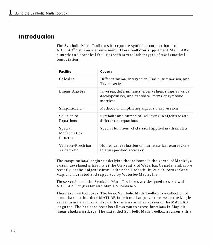
IntroductionThe Symbolic Math Toolboxes incorporate symbolic computation into MATLAB®’s numeric environment. These toolboxes supplement MATLAB’s numeric and graphical facilities with several other types of mathematical computation.
The computational engine underlying the toolboxes is the kernel of Maple®, a system developed primarily at the University of Waterloo, Canada, and, more recently, at the Eidgenössiche Technische Hochschule, Zürich, Switzerland. Maple is marketed and supported by Waterloo Maple, Inc.
These versions of the Symbolic Math Toolboxes are designed to work with MATLAB 6 or greater and Maple V Release 5.
There are two toolboxes. The basic Symbolic Math Toolbox is a collection of more than one-hundred MATLAB functions that provide access to the Maple kernel using a syntax and style that is a natural extension of the MATLAB language. The basic toolbox also allows you to access functions in Maple’s linear algebra package. The Extended Symbolic Math Toolbox augments this
Facility Covers
Calculus Differentiation, integration, limits, summation, and Taylor series
Linear Algebra Inverses, determinants, eigenvalues, singular value decomposition, and canonical forms of symbolic matrices
Simplification Methods of simplifying algebraic expressions
Solution of Equations
Symbolic and numerical solutions to algebraic and differential equations
Special Mathematical Functions
Special functions of classical applied mathematics
Variable-Precision Arithmetic
Numerical evaluation of mathematical expressions to any specified accuracy
1-3
functionality to include access to all nongraphics Maple packages, Maple programming features, and user-defined procedures. With both toolboxes, you can write your own M-files to access Maple functions and the Maple workspace.
The following sections of this Tutorial provide explanation and examples on how to use the toolboxes.
Chapter 2, “Reference” provides detailed descriptions of each of the functions in the toolboxes.
Section Covers
“Getting Help” How to get online help for Symbolic Math Toolbox functions
“Getting Started” Basic symbolic math operations
“Calculus” How to differentiate and integrate symbolic expressions
“Simplifications and Substitutions”
How to simplify and substitute values into expressions
“Variable-Precision Arithmetic”
How to control the precision of computations
“Linear Algebra” Examples using the toolbox functions
“Solving Equations” How to solve symbolic equations
“Special Mathematical Functions”
How to access Maple’s special math functions
“Using Maple Functions” How to use Maple’s help, debugging, and user-defined procedure functions
“Extended Symbolic Math Toolbox”
Features of the Extended Symbolic Math Toolbox
1 Using the Symbolic Math Toolbox
1-4
Getting HelpThere are several ways to find information on using Symbolic Math Toolbox functions. One, of course, is to read this manual! Another is to use online Help, which contains tutorials and reference information for all the functions. You can also use MATLAB’s command line help system. Generally, you can obtain help on MATLAB functions simply by typing
help function
where function is the name of the MATLAB function for which you need help. This is not sufficient, however, for some Symbolic Math Toolbox functions. The reason? The Symbolic Math Toolbox “overloads” many of MATLAB’s numeric functions. That is, it provides symbolic-specific implementations of the functions, using the same function name. To obtain help for the symbolic version of an overloaded function, type
help sym/function
where function is the overloaded function’s name. For example, to obtain help on the symbolic version of the overloaded function, diff, type
help sym/diff
To obtain information on the numeric version, simply type
help diff
How can you tell whether a function is overloaded? The help for the numeric version tells you so. For example, the help for the diff function contains the section
Overloaded methods help char/diff.m help sym/diff.m
This tells you that there are two other diff commands that operate on expressions of class char and class sym, respectively. See the next section for information on class sym. See the MATLAB topic “Programming and Data Types” for more information on overloaded commands.
You can use the mhelp command to obtain help on Maple commands. For example, to obtain help on the Maple diff command, type mhelp diff. This returns the help page for the Maple diff function. For more information on the
Getting Help
1-5
mhelp command, type help mhelp or read the section “Using Maple Functions” in this Tutorial.

1 Using the Symbolic Math Toolbox
1-6
Getting StartedThis section describes how to create and use symbolic objects. It also describes the default symbolic variable. If you are familiar with version 1 of the Symbolic Math Toolbox, please note that version 2 uses substantially different and simpler syntax.
(If you already have a copy of the Maple V Release 5 library, please see the reference page for mapleinit before proceeding.)
To get a quick online introduction to the Symbolic Math Toolbox, type demos at the MATLAB command line. MATLAB displays the MATLAB Demos dialog box. Select Symbolic Math (in the left list box) and then Introduction (in the right list box).
Symbolic ObjectsThe Symbolic Math Toolbox defines a new MATLAB data type called a symbolic object or sym (see the MATLAB topic “Programming and Data Types” for an introduction to MATLAB classes and objects). Internally, a symbolic
Getting Started
1-7
object is a data structure that stores a string representation of the symbol. The Symbolic Math Toolbox uses symbolic objects to represent symbolic variables, expressions, and matrices.
Creating Symbolic Variables and ExpressionsThe sym command lets you construct symbolic variables and expressions. For example, the commands
x = sym('x')a = sym('alpha')
create a symbolic variable x that prints as x and a symbolic variable a that prints as alpha.
Suppose you want to use a symbolic variable to represent the golden ratio
The command
rho = sym('(1 + sqrt(5))/2')
achieves this goal. Now you can perform various mathematical operations on rho. For example,
f = rho^2 - rho - 1
returns
f = (1/2+1/2*5^(1/2))^2-3/2-1/2*5^(1/2)
Then
simplify(f)
returns
0
Now suppose you want to study the quadratic function . The statement
ρ 1 5+2
-----------------=
f ax2 bx c+ +=
1 Using the Symbolic Math Toolbox
1-8
f = sym('a*x^2 + b*x + c')
assigns the symbolic expression to the variable f. Observe that in this case, the Symbolic Math Toolbox does not create variables corresponding to the terms of the expression, , , , and . To perform symbolic math operations (e.g., integration, differentiation, substitution, etc.) on f, you need to create the variables explicitly. You can do this by typing
a = sym('a')b = sym('b')c = sym('c')x = sym('x')
or simply
syms a b c x
In general, you can use sym or syms to create symbolic variables. We recommend you use syms because it requires less typing.
Symbolic and Numeric ConversionsConsider the ordinary MATLAB quantity
t = 0.1
The sym function has four options for returning a symbolic representation of the numeric value stored in t. The 'f' option
sym(t,'f')
returns a symbolic floating-point representation
'1.999999999999a'*2^(-4)
The 'r' option
sym(t,'r')
returns the rational form
1/10
This is the default setting for sym. That is, calling sym without a second argument is the same as using sym with the 'r' option.
ax2 bx c+ +
a b c x
Getting Started
1-9
sym(t) ans =1/10
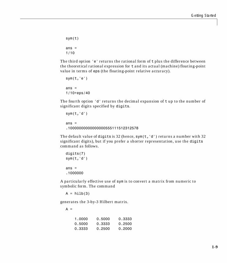
The third option 'e' returns the rational form of t plus the difference between the theoretical rational expression for t and its actual (machine) floating-point value in terms of eps (the floating-point relative accuracy).
sym(t,'e') ans =1/10+eps/40
The fourth option 'd' returns the decimal expansion of t up to the number of significant digits specified by digits.
sym(t,'d') ans =.10000000000000000555111512312578
The default value of digits is 32 (hence, sym(t,'d') returns a number with 32 significant digits), but if you prefer a shorter representation, use the digits command as follows.
digits(7)sym(t,'d') ans =.1000000
A particularly effective use of sym is to convert a matrix from numeric to symbolic form. The command
A = hilb(3)
generates the 3-by-3 Hilbert matrix.
A = 1.0000 0.5000 0.3333 0.5000 0.3333 0.2500 0.3333 0.2500 0.2000
1 Using the Symbolic Math Toolbox
1-10
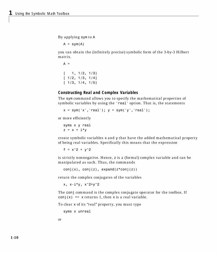
By applying sym to A
A = sym(A)
you can obtain the (infinitely precise) symbolic form of the 3-by-3 Hilbert matrix.
A = [ 1, 1/2, 1/3][ 1/2, 1/3, 1/4][ 1/3, 1/4, 1/5]
Constructing Real and Complex VariablesThe sym command allows you to specify the mathematical properties of symbolic variables by using the 'real' option. That is, the statements
x = sym('x','real'); y = sym('y','real');
or more efficiently
syms x y realz = x + i*y
create symbolic variables x and y that have the added mathematical property of being real variables. Specifically this means that the expression
f = x^2 + y^2
is strictly nonnegative. Hence, z is a (formal) complex variable and can be manipulated as such. Thus, the commands
conj(x), conj(z), expand(z*conj(z))
return the complex conjugates of the variables
x, x-i*y, x^2+y^2
The conj command is the complex conjugate operator for the toolbox. If conj(x) == x returns 1, then x is a real variable.
To clear x of its “real” property, you must type
syms x unreal
or
Getting Started
1-11
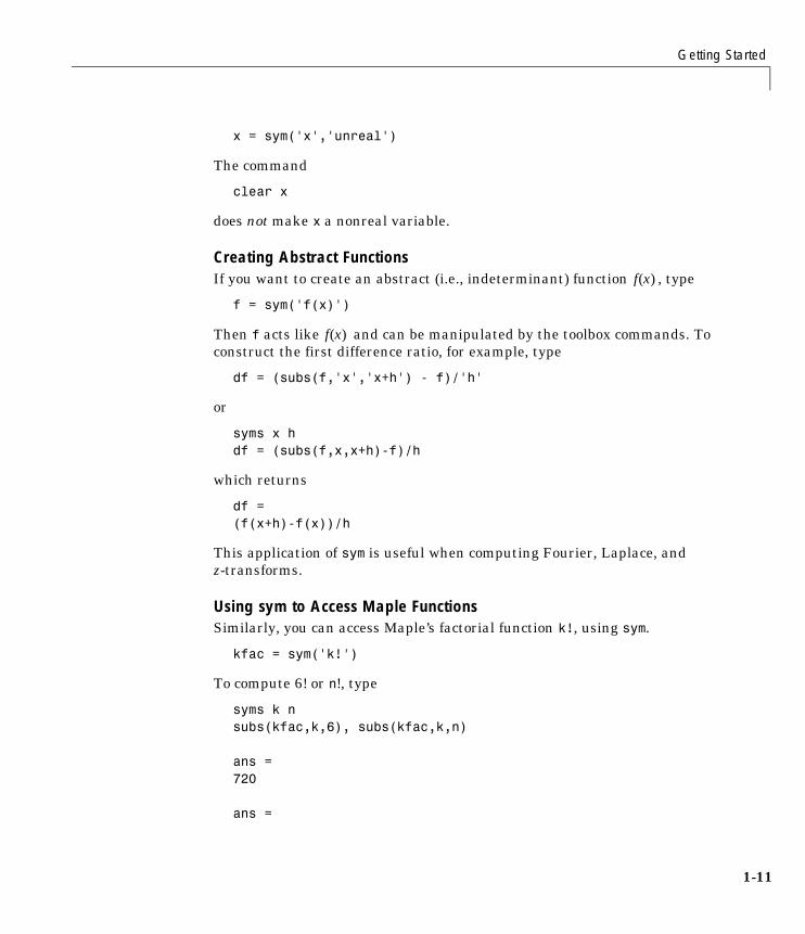
x = sym('x','unreal')
The command
clear x
does not make x a nonreal variable.
Creating Abstract FunctionsIf you want to create an abstract (i.e., indeterminant) function , type
f = sym('f(x)')
Then f acts like and can be manipulated by the toolbox commands. To construct the first difference ratio, for example, type
df = (subs(f,'x','x+h') - f)/'h'
or
syms x hdf = (subs(f,x,x+h)-f)/h
which returns
df =(f(x+h)-f(x))/h
This application of sym is useful when computing Fourier, Laplace, and z-transforms.
Using sym to Access Maple FunctionsSimilarly, you can access Maple’s factorial function k!, using sym.
kfac = sym('k!')
To compute 6! or n!, type
syms k nsubs(kfac,k,6), subs(kfac,k,n) ans =720
ans =
f x( )
f x( )
1 Using the Symbolic Math Toolbox
1-12
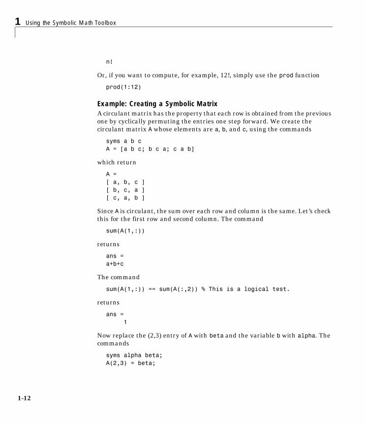
n!
Or, if you want to compute, for example, 12!, simply use the prod function
prod(1:12)
Example: Creating a Symbolic MatrixA circulant matrix has the property that each row is obtained from the previous one by cyclically permuting the entries one step forward. We create the circulant matrix A whose elements are a, b, and c, using the commands
syms a b cA = [a b c; b c a; c a b]
which return
A = [ a, b, c ][ b, c, a ][ c, a, b ]
Since A is circulant, the sum over each row and column is the same. Let’s check this for the first row and second column. The command
sum(A(1,:))
returns
ans =a+b+c
The command
sum(A(1,:)) == sum(A(:,2)) % This is a logical test.
returns
ans = 1
Now replace the (2,3) entry of A with beta and the variable b with alpha. The commands
syms alpha beta;A(2,3) = beta;
Getting Started
1-13
A = subs(A,b,alpha)
return
A = [ a, alpha, c][ alpha, c, beta][ c, a, alpha]
From this example, you can see that using symbolic objects is very similar to using regular MATLAB numeric objects.
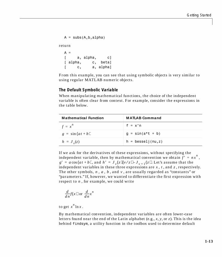
The Default Symbolic VariableWhen manipulating mathematical functions, the choice of the independent variable is often clear from context. For example, consider the expressions in the table below.
If we ask for the derivatives of these expressions, without specifying the independent variable, then by mathematical convention we obtain ,
, and . Let’s assume that the independent variables in these three expressions are , , and , respectively. The other symbols, , , , and , are usually regarded as “constants” or “parameters.” If, however, we wanted to differentiate the first expression with respect to , for example, we could write
to get .
By mathematical convention, independent variables are often lower-case letters found near the end of the Latin alphabet (e.g., x, y, or z). This is the idea behind findsym, a utility function in the toolbox used to determine default
Mathematical Function MATLAB Command
f = x^n
g = sin(a*t + b)
h = besselj(nu,z)
f xn=
g at b+( )sin=
h Jv z( )=
f ′ nxn=
g′ a at b+( )cos= h′ Jv z( ) v z⁄( ) Jv 1+ z( )–=x t z
n a b v
n
or ddn-------f x( ) d
dn-------xn
xn xln
1 Using the Symbolic Math Toolbox
1-14
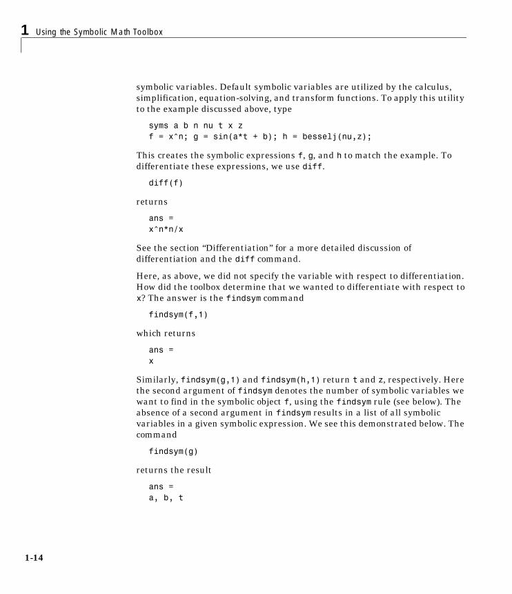
symbolic variables. Default symbolic variables are utilized by the calculus, simplification, equation-solving, and transform functions. To apply this utility to the example discussed above, type
syms a b n nu t x zf = x^n; g = sin(a*t + b); h = besselj(nu,z);
This creates the symbolic expressions f, g, and h to match the example. To differentiate these expressions, we use diff.
diff(f)
returns
ans =x^n*n/x
See the section “Differentiation” for a more detailed discussion of differentiation and the diff command.
Here, as above, we did not specify the variable with respect to differentiation. How did the toolbox determine that we wanted to differentiate with respect to x? The answer is the findsym command
findsym(f,1)
which returns
ans =x
Similarly, findsym(g,1) and findsym(h,1) return t and z, respectively. Here the second argument of findsym denotes the number of symbolic variables we want to find in the symbolic object f, using the findsym rule (see below). The absence of a second argument in findsym results in a list of all symbolic variables in a given symbolic expression. We see this demonstrated below. The command
findsym(g)
returns the result
ans =a, b, t
Getting Started
1-15
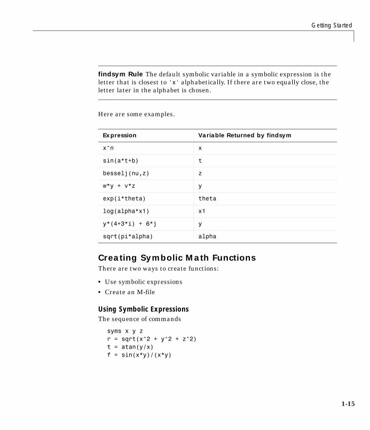
findsym Rule The default symbolic variable in a symbolic expression is the letter that is closest to 'x' alphabetically. If there are two equally close, the letter later in the alphabet is chosen.
Here are some examples.
Creating Symbolic Math FunctionsThere are two ways to create functions:
• Use symbolic expressions
• Create an M-file
Using Symbolic ExpressionsThe sequence of commands
syms x y zr = sqrt(x^2 + y^2 + z^2)t = atan(y/x)f = sin(x*y)/(x*y)
Expression Variable Returned by findsym
x^n x
sin(a*t+b) t
besselj(nu,z) z
w*y + v*z y
exp(i*theta) theta
log(alpha*x1) x1
y*(4+3*i) + 6*j y
sqrt(pi*alpha) alpha

1 Using the Symbolic Math Toolbox
1-16
generates the symbolic expressions r, t, and f. You can use diff, int, subs, and other Symbolic Math Toolbox functions to manipulate such expressions.
Creating an M-FileM-files permit a more general use of functions. Suppose, for example, you want to create the sinc function sin(x)/x. To do this, create an M-file in the @sym directory.
function z = sinc(x)%SINC The symbolic sinc function% sin(x)/x. This function% accepts a sym as the input argument.if isequal(x,sym(0)) z = 1;else z = sin(x)/x;end
You can extend such examples to functions of several variables. See the MATLAB topic “Programming and Data Types” for a more detailed discussion on object-oriented programming.
Calculus
1-17
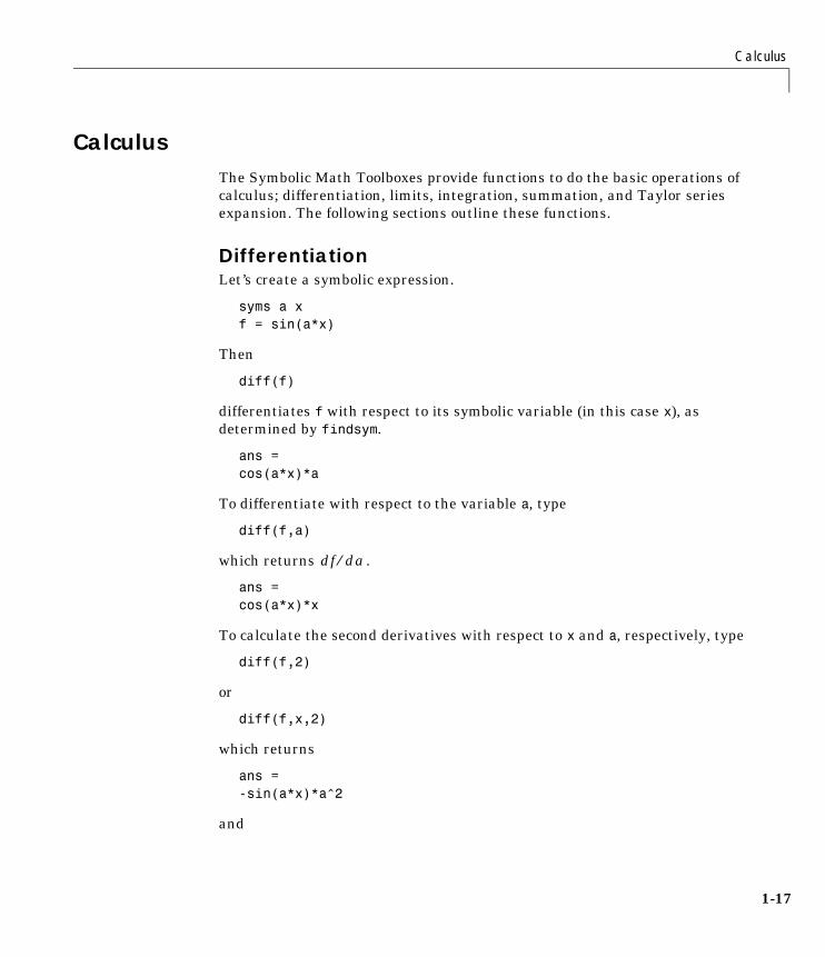
CalculusThe Symbolic Math Toolboxes provide functions to do the basic operations of calculus; differentiation, limits, integration, summation, and Taylor series expansion. The following sections outline these functions.
DifferentiationLet’s create a symbolic expression.
syms a x f = sin(a*x)
Then
diff(f)
differentiates f with respect to its symbolic variable (in this case x), as determined by findsym.
ans =cos(a*x)*a
To differentiate with respect to the variable a, type
diff(f,a)
which returns .
ans =cos(a*x)*x
To calculate the second derivatives with respect to x and a, respectively, type
diff(f,2)
or
diff(f,x,2)
which returns
ans =-sin(a*x)*a^2
and
df da⁄
1 Using the Symbolic Math Toolbox
1-18
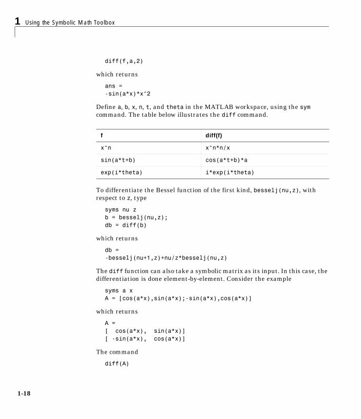
diff(f,a,2)
which returns
ans =-sin(a*x)*x^2
Define a, b, x, n, t, and theta in the MATLAB workspace, using the sym command. The table below illustrates the diff command.
To differentiate the Bessel function of the first kind, besselj(nu,z), with respect to z, type
syms nu zb = besselj(nu,z);db = diff(b)
which returns
db =-besselj(nu+1,z)+nu/z*besselj(nu,z)
The diff function can also take a symbolic matrix as its input. In this case, the differentiation is done element-by-element. Consider the example
syms a xA = [cos(a*x),sin(a*x);-sin(a*x),cos(a*x)]
which returns
A =[ cos(a*x), sin(a*x)][ -sin(a*x), cos(a*x)]
The command
diff(A)
f diff(f)
x^n x^n*n/x
sin(a*t+b) cos(a*t+b)*a
exp(i*theta) i*exp(i*theta)
Calculus
1-19
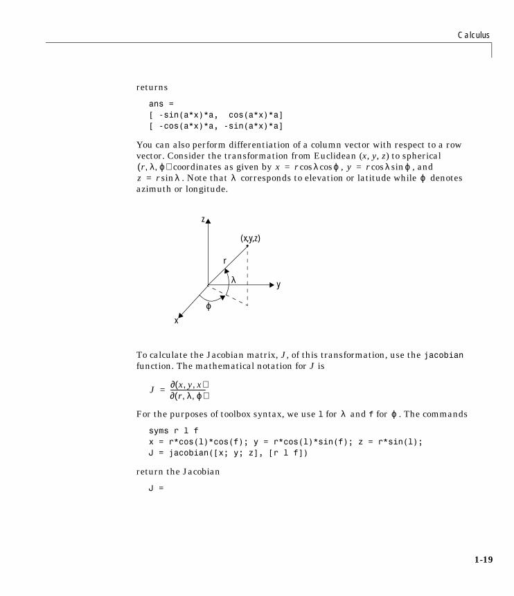
returns
ans =[ -sin(a*x)*a, cos(a*x)*a][ -cos(a*x)*a, -sin(a*x)*a]
You can also perform differentiation of a column vector with respect to a row vector. Consider the transformation from Euclidean (x, y, z) to spherical
coordinates as given by , , and . Note that corresponds to elevation or latitude while denotes
azimuth or longitude.
To calculate the Jacobian matrix, J, of this transformation, use the jacobian function. The mathematical notation for J is
For the purposes of toolbox syntax, we use l for and f for . The commands
syms r l fx = r*cos(l)*cos(f); y = r*cos(l)*sin(f); z = r*sin(l);J = jacobian([x; y; z], [r l f])
return the Jacobian
J =
r λ ϕ, ,( ) x r λ ϕcoscos= y r λ ϕsincos=z r λsin= λ ϕ
z
y
x
(x,y,z)
ϕ
λ
r
J x y x, ,( )∂r λ ϕ, ,( )∂
-----------------------=
λ ϕ

1 Using the Symbolic Math Toolbox
1-20
[ cos(l)*cos(f), -r*sin(l)*cos(f), -r*cos(l)*sin(f)][ cos(l)*sin(f), -r*sin(l)*sin(f), r*cos(l)*cos(f)][ sin(l), r*cos(l), 0]
and the command
detJ = simple(det(J))
returns
detJ = -cos(l)*r^2
Notice that the first argument of the jacobian function must be a column vector and the second argument a row vector. Moreover, since the determinant of the Jacobian is a rather complicated trigonometric expression, we used the simple command to make trigonometric substitutions and reductions (simplifications). The section “Simplifications and Substitutions” discusses simplification in more detail.
A table summarizing diff and jacobian follows.
LimitsThe fundamental idea in calculus is to make calculations on functions as a variable “gets close to” or approaches a certain value. Recall that the definition of the derivative is given by a limit
Mathematical Operator MATLAB Command
diff(f) or diff(f,x)
diff(f,a)
diff(f,b,2)
J = jacobian([r:t],[u,v])
dfdx-------
dfda-------
d2f
db2----------
J r t,( )∂u v,( )∂
-----------------=

Calculus
1-21
provided this limit exists. The Symbolic Math Toolbox allows you to compute the limits of functions in a direct manner. The commands
syms h n xlimit( (cos(x+h) - cos(x))/h,h,0 )
which return
ans =-sin(x)
and
limit( (1 + x/n)^n,n,inf )
which returns
ans =exp(x)
illustrate two of the most important limits in mathematics: the derivative (in this case of cos x) and the exponential function. While many limits
are “two sided” (that is, the result is the same whether the approach is from the right or left of a), limits at the singularities of are not. Hence, the three limits
yield the three distinct results: undefined, , and , respectively.
In the case of undefined limits, the Symbolic Math Toolbox returns NaN (not a number). The command
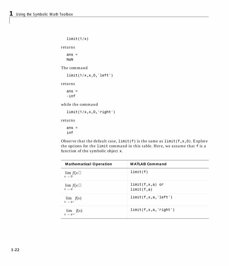
limit(1/x,x,0)
or
f ′ x( ) f x h+( ) f x( )–h
----------------------------------h 0→lim=
f x( )x a→lim
f x( )
, , and 1x---
x 0→lim 1
x---
x 0-→lim 1
x---
x 0+→lim
∞– +∞
1 Using the Symbolic Math Toolbox
1-22
limit(1/x)
returns
ans =NaN
The command
limit(1/x,x,0,'left')
returns
ans =-inf
while the command
limit(1/x,x,0,'right')
returns
ans =inf
Observe that the default case, limit(f) is the same as limit(f,x,0). Explore the options for the limit command in this table. Here, we assume that f is a function of the symbolic object x.
Mathematical Operation MATLAB Command
limit(f)
limit(f,x,a) orlimit(f,a)
limit(f,x,a,'left')
limit(f,x,a,'right')
f x( )x 0→lim
f x( )x a→lim
f x( )x a-→lim
f x( )x a+→lim
Calculus
1-23
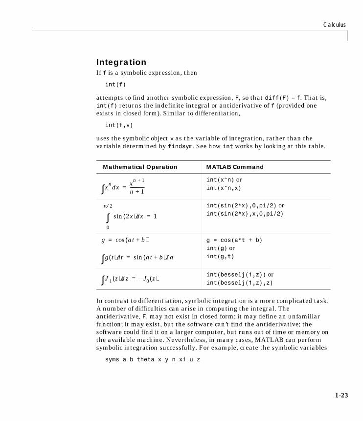
IntegrationIf f is a symbolic expression, then
int(f)
attempts to find another symbolic expression, F, so that diff(F) = f. That is, int(f) returns the indefinite integral or antiderivative of f (provided one exists in closed form). Similar to differentiation,
int(f,v)
uses the symbolic object v as the variable of integration, rather than the variable determined by findsym. See how int works by looking at this table.
In contrast to differentiation, symbolic integration is a more complicated task. A number of difficulties can arise in computing the integral. The antiderivative, F, may not exist in closed form; it may define an unfamiliar function; it may exist, but the software can’t find the antiderivative; the software could find it on a larger computer, but runs out of time or memory on the available machine. Nevertheless, in many cases, MATLAB can perform symbolic integration successfully. For example, create the symbolic variables
syms a b theta x y n x1 u z
Mathematical Operation MATLAB Command
int(x^n) orint(x^n,x)
int(sin(2*x),0,pi/2) or int(sin(2*x),x,0,pi/2)
g = cos(a*t + b)int(g) orint(g,t)
int(besselj(1,z)) orint(besselj(1,z),z)
xn xd∫ xn 1+
n 1+-------------=
2x( )sin xd
0
π 2⁄
∫ 1=
g at b+( )cos=
g t( ) td∫ at b+( )sin a⁄=
J1 z( )∫ dz J– 0 z( )=

1 Using the Symbolic Math Toolbox
1-24
These tables illustrate integration of expressions containing those variables.
The last example shows what happens if the toolbox can’t find the antiderivative; it simply returns the command, including the variable of integration, unevaluated.
Definite integration is also possible. The commands
int(f,a,b)
and
int(f,v,a,b)
are used to find a symbolic expression for
respectively.
Here are some additional examples.
f int(f)
x^n x^(n+1)/(n+1)
y^(-1) log(y)
n^x 1/log(n)*n^x
sin(a*theta+b) -1/a*cos(a*theta+b)
exp(-x1^2) 1/2*pi^(1/2)*erf(x1)
1/(1+u^2) atan(u)
f a, b int(f,a,b)
x^7 0, 1 1/8
1/x 1, 2 log(2)
and f x( )a
b
∫ dx f v( ) vda
b
∫

Calculus
1-25
For the Bessel function (besselj) example, it is possible to compute a numerical approximation to the value of the integral, using the double function. The command
a = int(besselj(1,z),0,1)
returns
a =1/4*hypergeom([1],[2, 2],-1/4)
and the command
a = double(a)
returns
a = 0.2348
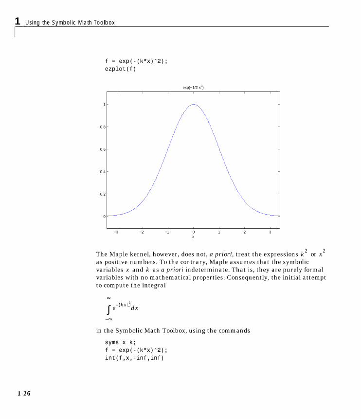
Integration with Real ConstantsOne of the subtleties involved in symbolic integration is the “value” of various parameters. For example, the expression
is the positive, bell shaped curve that tends to 0 as x tends to for any real number k. An example of this curve is depicted below with
and generated, using these commands.
syms xk = sym(1/sqrt(2));
log(x)*sqrt(x) 0, 1 -4/9
exp(-x^2) 0, inf 1/2*pi^(1/2)
besselj(1,z) 0, 1 1/4*hypergeom([1],[2, 2],-1/4)
f a, b int(f,a,b)
e kx( )– 2
∞±
k 12
-------=
1 Using the Symbolic Math Toolbox
1-26
f = exp(-(k*x)^2);ezplot(f)
The Maple kernel, however, does not, a priori, treat the expressions or as positive numbers. To the contrary, Maple assumes that the symbolic variables and as a priori indeterminate. That is, they are purely formal variables with no mathematical properties. Consequently, the initial attempt to compute the integral
in the Symbolic Math Toolbox, using the commands
syms x k;f = exp(-(k*x)^2);int(f,x,-inf,inf)
−3 −2 −1 0 1 2 3
0
0.2
0.4
0.6
0.8
1
x
exp(−1/2 x2)
k2 x2
x k
e kx( )– 2
∞–
∞
∫ dx

Calculus
1-27
results in the output
Definite integration: Can't determine if the integral is convergent.Need to know the sign of --> k^2Will now try indefinite integration and then take limits.
Warning: Explicit integral could not be found.ans =int(exp(-k^2*x^2),x= -inf..inf)
In the next section, you will see how to make a real variable and therefore positive.
Real Variables via symNotice that Maple is not able to determine the sign of the expression k^2. How does one surmount this obstacle? The answer is to make k a real variable, using the sym command. One particularly useful feature of sym, namely the real option, allows you to declare k to be a real variable. Consequently, the integral above is computed, in the toolbox, using the sequence
syms k realint(f,x,-inf,inf)
which returns
ans =signum(k)/k*pi^(1/2)
Notice that k is now a symbolic object in the MATLAB workspace and a real variable in the Maple kernel workspace. By typing
clear k
you only clear k in the MATLAB workspace. To ensure that k has no formal properties (that is, to ensure k is a purely formal variable), type
syms k unreal
This variation of the syms command clears k in the Maple workspace. You can also declare a sequence of symbolic variables w, y, x, z to be real, using
syms w x y z real
kk2
1 Using the Symbolic Math Toolbox
1-28
In this case, all of the variables in between the words syms and real are assigned the property real. That is, they are real variables in the Maple workspace.
Symbolic SummationYou can compute symbolic summations, when they exist, by using the symsum command. For example, the p-series
adds to , while the geometric series adds to , provided . Three summations are demonstrated below.
syms x ks1 = symsum(1/k^2,1,inf)s2 = symsum(x^k,k,0,inf)
s1 = 1/6*pi^2
s2 = -1/(x-1)
1 1
22------ 1
32------ …+ + +
π2 6⁄ 1 x x2 …+ + + 1 1 x–( )⁄x 1<
Calculus
1-29
Taylor SeriesThe statements
syms xf = 1/(5+4*cos(x))T = taylor(f,8)
return
T =1/9+2/81*x^2+5/1458*x^4+49/131220*x^6
which is all the terms up to, but not including, order eight in the Taylor series for .
Technically, T is a Maclaurin series, since its basepoint is a = 0.
The command
pretty(T)
prints T in a format resembling typeset mathematics.
2 4 49 61/9 + 2/81 x + 5/1458 x + ------ x 131220
These commands
syms xg = exp(x*sin(x))t = taylor(g,12,2);
generate the first 12 nonzero terms of the Taylor series for g about x = 2.
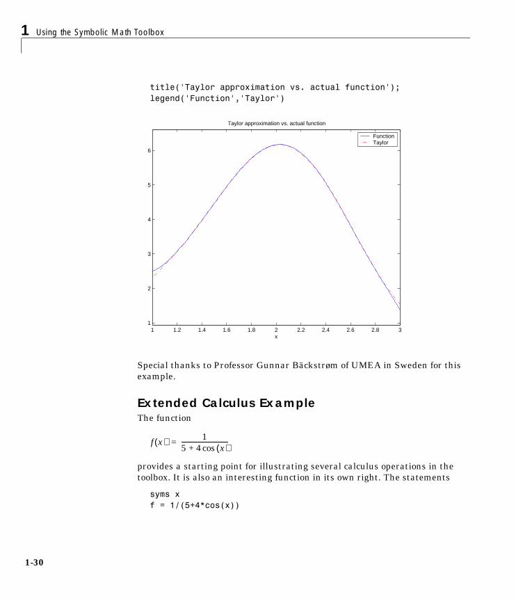
Let’s plot these functions together to see how well this Taylor approximation compares to the actual function g.
xd = 1:0.05:3; yd = subs(g,x,xd);ezplot(t, [1,3]); hold on;plot(xd, yd, 'r-.')
O x8( )( )f x( )
x a–( )n
n 0=
∞
∑ f n( ) a( )n!
-----------------
1 Using the Symbolic Math Toolbox
1-30
title('Taylor approximation vs. actual function');legend('Function','Taylor')
Special thanks to Professor Gunnar Bäckstrøm of UMEA in Sweden for this example.
Extended Calculus Example The function
provides a starting point for illustrating several calculus operations in the toolbox. It is also an interesting function in its own right. The statements
syms x f = 1/(5+4*cos(x))
1 1.2 1.4 1.6 1.8 2 2.2 2.4 2.6 2.8 31
2
3
4
5
6
x
Taylor approximation vs. actual function
FunctionTaylor
f x( ) 15 4 x( )cos+------------------------------=
Calculus
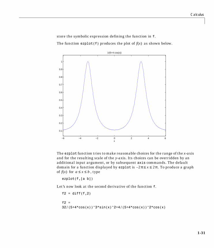
1-31
store the symbolic expression defining the function in f.
The function ezplot(f) produces the plot of as shown below.
The ezplot function tries to make reasonable choices for the range of the x-axis and for the resulting scale of the y-axis. Its choices can be overridden by an additional input argument, or by subsequent axis commands. The default domain for a function displayed by ezplot is . To produce a graph of for , type
ezplot(f,[a b])
Let’s now look at the second derivative of the function f.
f2 = diff(f,2)
f2 =32/(5+4*cos(x))^3*sin(x)^2+4/(5+4*cos(x))^2*cos(x)
f x( )
−6 −4 −2 0 2 4 6
0.1
0.2
0.3
0.4
0.5
0.6
0.7
0.8
0.9
1
x
1/(5+4 cos(x))
2π– x 2π≤ ≤f x( ) a x b≤ ≤
1 Using the Symbolic Math Toolbox
1-32
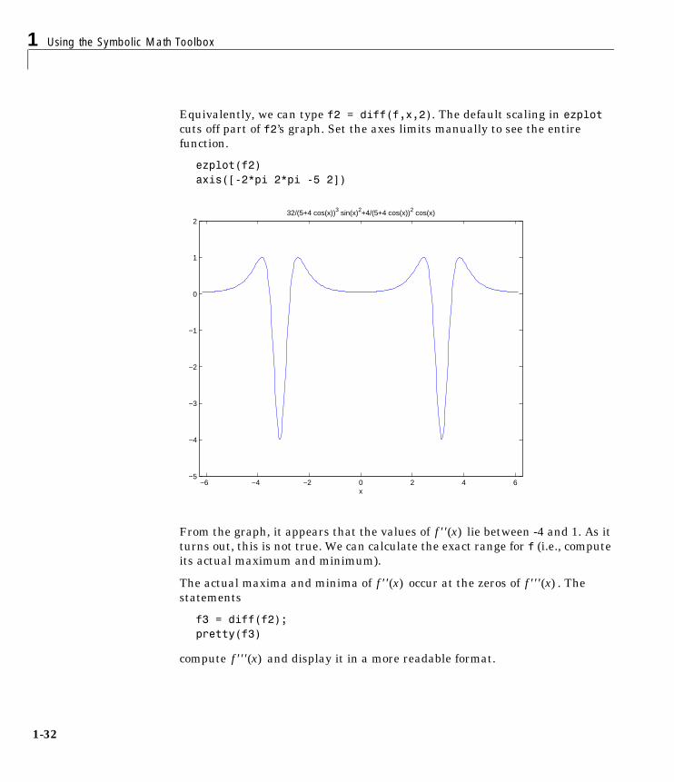
Equivalently, we can type f2 = diff(f,x,2). The default scaling in ezplot cuts off part of f2’s graph. Set the axes limits manually to see the entire function.
ezplot(f2) axis([-2*pi 2*pi -5 2])
From the graph, it appears that the values of lie between -4 and 1. As it turns out, this is not true. We can calculate the exact range for f (i.e., compute its actual maximum and minimum).
The actual maxima and minima of occur at the zeros of . The statements
f3 = diff(f2);pretty(f3)
compute and display it in a more readable format.
−6 −4 −2 0 2 4 6−5
−4
−3
−2
−1
0
1
2
x
32/(5+4 cos(x))3 sin(x)2+4/(5+4 cos(x))2 cos(x)
f ′′ x( )
f ′′ x( ) f ′′′ x( )
f ′′′ x( )
Calculus
1-33
3sin(x) sin(x) cos(x) sin(x)
384 --------------- + 96 --------------- - 4 ---------------4 3 2
(5 + 4 cos(x)) (5 + 4 cos(x)) (5 + 4 cos(x))
We can simplify this expression using the statements
f3 = simple(f3);pretty(f3)
2 2 sin(x) (96 sin(x) + 80 cos(x) + 80 cos(x) - 25) 4 ------------------------------------------------- 4 (5 + 4 cos(x))
Now use the solve function to find the zeros of .
z = solve(f3)
returns a 5-by-1 symbolic matrix
z =[ 0][ atan((-255-60*19^(1/2))^(1/2),10+3*19^(1/2))][ atan(-(-255-60*19^(1/2))^(1/2),10+3*19^(1/2))][ atan((-255+60*19^(1/2))^(1/2)/(10-3*19^(1/2)))+pi][ -atan((-255+60*19^(1/2))^(1/2)/(10-3*19^(1/2)))-pi]
each of whose entries is a zero of . The commands
format; % Default format of 5 digitszr = double(z)
convert the zeros to double form.
f ′′′ x( )
f ′′′ x( )
1 Using the Symbolic Math Toolbox
1-34
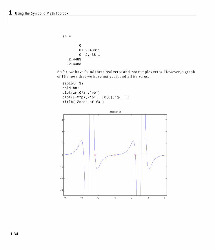
zr = 0 0+ 2.4381i 0- 2.4381i 2.4483 -2.4483
So far, we have found three real zeros and two complex zeros. However, a graph of f3 shows that we have not yet found all its zeros.
ezplot(f3)hold on;plot(zr,0*zr,'ro')plot([-2*pi,2*pi], [0,0],'g-.');title('Zeros of f3')
−6 −4 −2 0 2 4 6
−3
−2
−1
0
1
2
3
x
Zeros of f3
Calculus
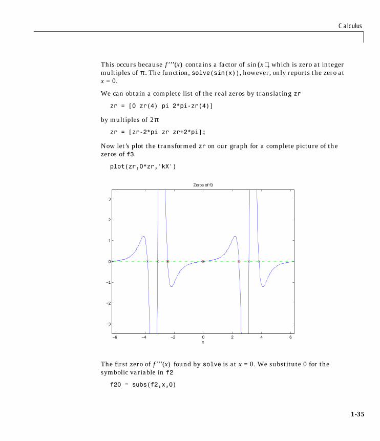
1-35
This occurs because contains a factor of , which is zero at integer multiples of . The function, solve(sin(x)), however, only reports the zero at x = 0.
We can obtain a complete list of the real zeros by translating zr
zr = [0 zr(4) pi 2*pi-zr(4)]
by multiples of
zr = [zr-2*pi zr zr+2*pi];
Now let’s plot the transformed zr on our graph for a complete picture of the zeros of f3.
plot(zr,0*zr,'kX')
The first zero of found by solve is at x = 0. We substitute 0 for the symbolic variable in f2
f20 = subs(f2,x,0)
f ′′′ x( ) x( )sinπ
2π
−6 −4 −2 0 2 4 6
−3
−2
−1
0
1
2
3
x
Zeros of f3
f ′′′ x( )
1 Using the Symbolic Math Toolbox
1-36
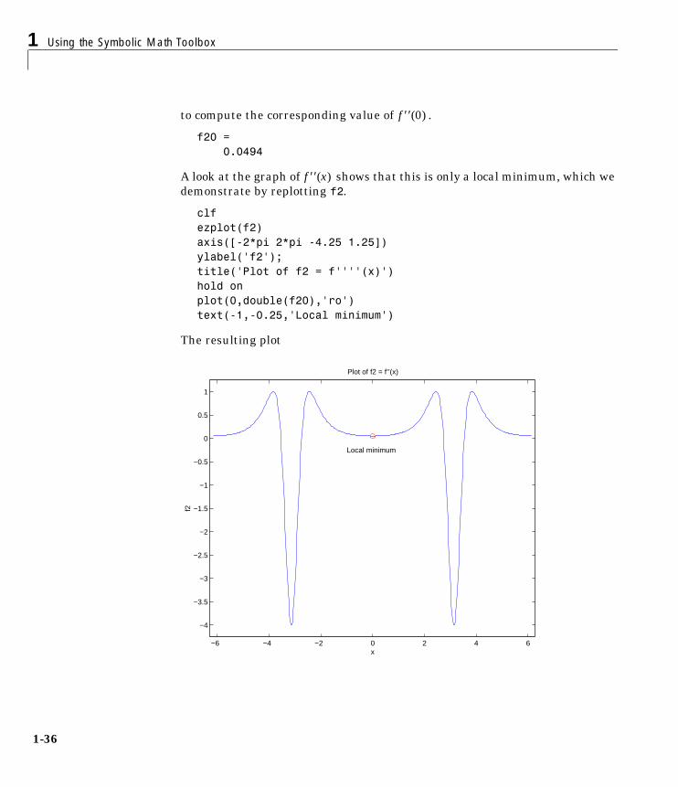
to compute the corresponding value of .
f20 = 0.0494
A look at the graph of shows that this is only a local minimum, which we demonstrate by replotting f2.
clfezplot(f2)axis([-2*pi 2*pi -4.25 1.25])ylabel('f2');title('Plot of f2 = f''''(x)')hold onplot(0,double(f20),'ro') text(-1,-0.25,'Local minimum')
The resulting plot
f ′′ 0( )
f ′′ x( )
−6 −4 −2 0 2 4 6
−4
−3.5
−3
−2.5
−2
−1.5
−1
−0.5
0
0.5
1
x
Plot of f2 = f’’(x)
f2
Local minimum

Calculus
1-37
indicates that the global minima occur near and . We can demonstrate that they occur exactly at , using the following sequence of commands. First we try substituting and into .
simple([subs(f3,x,-sym(pi)),subs(f3,x,sym(pi))])
The result
ans =[ 0, 0]
shows that and happen to be critical points of . We can see that and are global minima by plotting f2(-pi) and f2(pi) against f2(x).
m1 = double(subs(f2,x,-pi)); m2 = double(subs(f2,x,pi));plot(-pi,m1,'go',pi,m2,'go')text(-1,-4,'Global minima')
The actual minima are m1, m2
ans = [ -4, -4]
as shown in the following plot.
x π–= x π=x π±=π– π f ′′′ x( )
π– π f ′′′ x( ) π–π
1 Using the Symbolic Math Toolbox
1-38
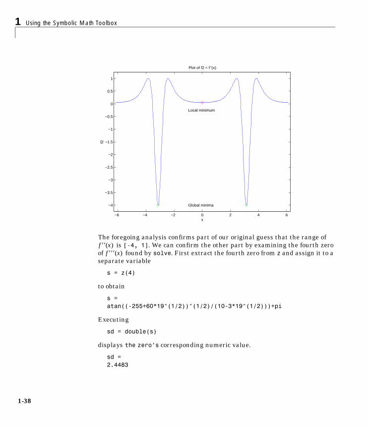
The foregoing analysis confirms part of our original guess that the range of is [-4, 1]. We can confirm the other part by examining the fourth zero
of found by solve. First extract the fourth zero from z and assign it to a separate variable
s = z(4)
to obtain
s =atan((-255+60*19^(1/2))^(1/2)/(10-3*19^(1/2)))+pi
Executing
sd = double(s)
displays the zero’s corresponding numeric value.
sd =2.4483
−6 −4 −2 0 2 4 6
−4
−3.5
−3
−2.5
−2
−1.5
−1
−0.5
0
0.5
1
x
Plot of f2 = f’’(x)
f2
Local minimum
Global minima
f ′′ x( )f ′′′ x( )
Calculus
1-39
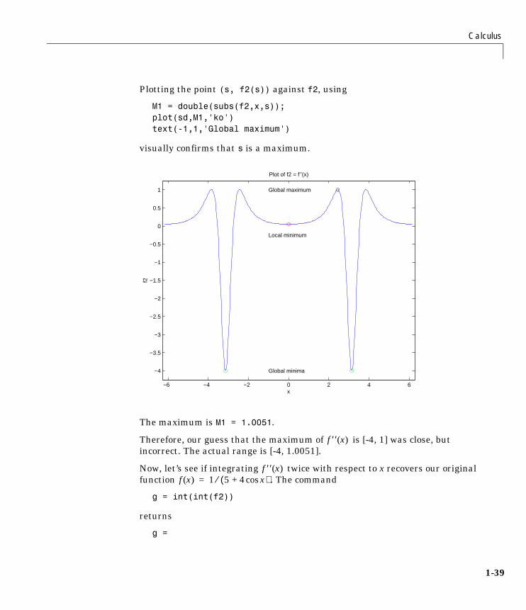
Plotting the point (s, f2(s)) against f2, using
M1 = double(subs(f2,x,s));plot(sd,M1,'ko')text(-1,1,'Global maximum')
visually confirms that s is a maximum.
The maximum is M1 = 1.0051.
Therefore, our guess that the maximum of is [-4, 1] was close, but incorrect. The actual range is [-4, 1.0051].
Now, let’s see if integrating twice with respect to x recovers our original function . The command
g = int(int(f2))
returns
g =
−6 −4 −2 0 2 4 6
−4
−3.5
−3
−2.5
−2
−1.5
−1
−0.5
0
0.5
1
x
Plot of f2 = f’’(x)
f2
Local minimum
Global minima
Global maximum
f ′′ x( )
f ′′ x( )f x( ) 1 5 4 xcos+( )⁄=
1 Using the Symbolic Math Toolbox
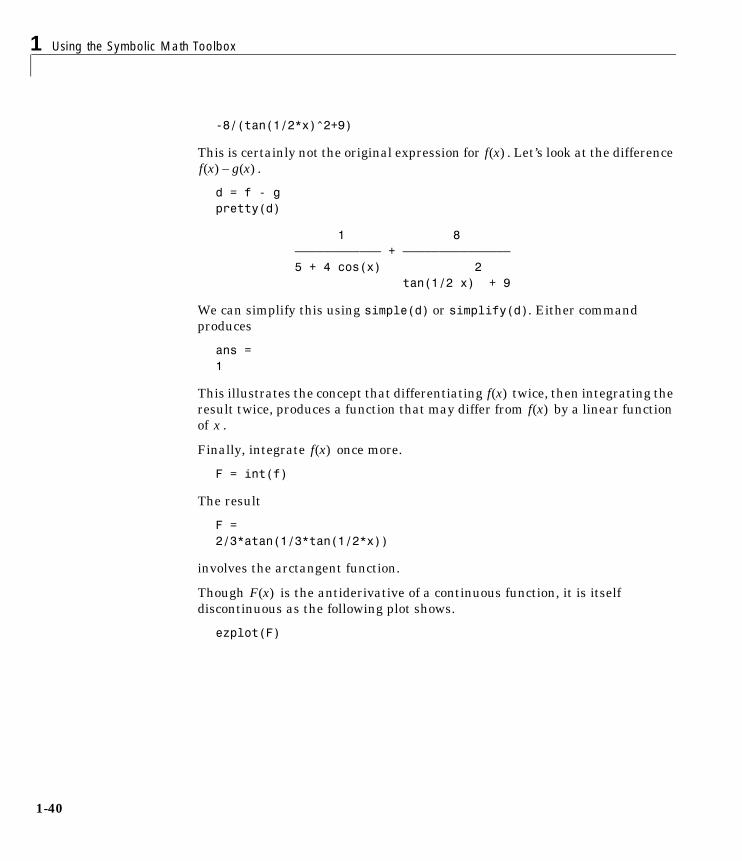
1-40
-8/(tan(1/2*x)^2+9)
This is certainly not the original expression for . Let’s look at the difference .
d = f - gpretty(d)
1 8 –––––––––––– + ––––––––––––––– 5 + 4 cos(x) 2 tan(1/2 x) + 9
We can simplify this using simple(d) or simplify(d). Either command produces
ans =1
This illustrates the concept that differentiating twice, then integrating the result twice, produces a function that may differ from by a linear function of .
Finally, integrate once more.
F = int(f)
The result
F =2/3*atan(1/3*tan(1/2*x))
involves the arctangent function.
Though is the antiderivative of a continuous function, it is itself discontinuous as the following plot shows.
ezplot(F)
f x( )f x( ) g x( )–
f x( )f x( )
x
f x( )
F x( )

Calculus
1-41
Note that has jumps at . This occurs because is singular at .
−6 −4 −2 0 2 4 6
−1
−0.8
−0.6
−0.4
−0.2
0
0.2
0.4
0.6
0.8
1
x
2/3 atan(1/3 tan(1/2 x))
F x( ) x π±= xtanx π±=

1 Using the Symbolic Math Toolbox
1-42
In fact, as
ezplot(atan(tan(x)))
shows, the numerical value of atan(tan(x))differs from x by a piecewise constant function that has jumps at odd multiples of .
To obtain a representation of that does not have jumps at these points, we must introduce a second function, , that compensates for the discontinuities. Then we add the appropriate multiple of to
J = sym('round(x/(2*pi))');c = sym('2/3*pi');F1 = F+c*JF1 =2/3*atan(1/3*tan(1/2*x))+2/3*pi*round(1/2*x/pi)
π 2⁄
−6 −4 −2 0 2 4 6
−1.5
−1
−0.5
0
0.5
1
1.5
x
atan(tan(x))
F x( )J x( )
J x( ) F x( )

Calculus
1-43
and plot the result.
ezplot(F1,[-6.28,6.28])
This representation does have a continuous graph.
Notice that we use the domain [-6.28, 6.28] in ezplot rather than the default domain . The reason for this is to prevent an evaluation of
at the singular points and where the jumps in F and J do not cancel out one another. The proper handling of branch cut discontinuities in multivalued functions like arctan x is a deep and difficult problem in symbolic computation. Although MATLAB and Maple cannot do this entirely automatically, they do provide the tools for investigating such questions.
−6 −4 −2 0 2 4 6−2.5
−2
−1.5
−1
−0.5
0
0.5
1
1.5
2
2.5
x
2/3 atan(1/3 tan(1/2 x))+2/3 π round(1/2 x/π)
2π– 2π[ , ]F1 2 3⁄ 1 3⁄ 1 2⁄ xtan( )atan= x π–= x π=
1 Using the Symbolic Math Toolbox
1-44
Simplifications and SubstitutionsThere are several functions that simplify symbolic expressions and are used to perform symbolic substitutions.
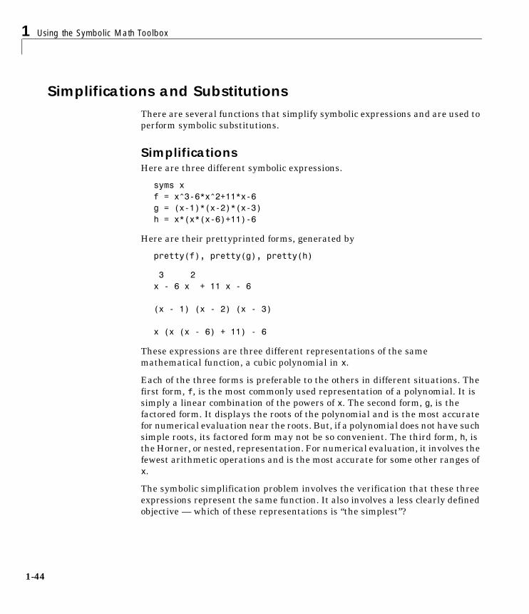
SimplificationsHere are three different symbolic expressions.
syms xf = x^3-6*x^2+11*x-6g = (x-1)*(x-2)*(x-3)h = x*(x*(x-6)+11)-6
Here are their prettyprinted forms, generated by
pretty(f), pretty(g), pretty(h)
3 2x - 6 x + 11 x - 6
(x - 1) (x - 2) (x - 3)
x (x (x - 6) + 11) - 6
These expressions are three different representations of the same mathematical function, a cubic polynomial in x.
Each of the three forms is preferable to the others in different situations. The first form, f, is the most commonly used representation of a polynomial. It is simply a linear combination of the powers of x. The second form, g, is the factored form. It displays the roots of the polynomial and is the most accurate for numerical evaluation near the roots. But, if a polynomial does not have such simple roots, its factored form may not be so convenient. The third form, h, is the Horner, or nested, representation. For numerical evaluation, it involves the fewest arithmetic operations and is the most accurate for some other ranges of x.
The symbolic simplification problem involves the verification that these three expressions represent the same function. It also involves a less clearly defined objective — which of these representations is “the simplest”?

Simplifications and Substitutions
1-45
This toolbox provides several functions that apply various algebraic and trigonometric identities to transform one representation of a function into another, possibly simpler, representation. These functions are collect, expand, horner, factor, simplify, and simple.
collectThe statement
collect(f)
views f as a polynomial in its symbolic variable, say x, and collects all the coefficients with the same power of x. A second argument can specify the variable in which to collect terms if there is more than one candidate. Here are a few examples.
f collect(f)
(x-1)*(x-2)*(x-3) x^3-6*x^2+11*x-6
x*(x*(x-6)+11)-6 x^3-6*x^2+11*x-6
(1+x)*t + x*t 2*x*t+t
1 Using the Symbolic Math Toolbox
1-46
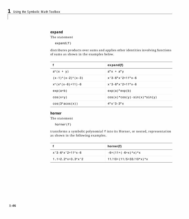
expandThe statement
expand(f)
distributes products over sums and applies other identities involving functions of sums as shown in the examples below.
hornerThe statement
horner(f)
transforms a symbolic polynomial f into its Horner, or nested, representation as shown in the following examples.
f expand(f)
a∗(x + y) a∗x + a∗y
(x-1)∗(x-2)∗(x-3) x^3-6∗x^2+11∗x-6
x∗(x∗(x-6)+11)-6 x^3-6∗x^2+11∗x-6
exp(a+b) exp(a)∗exp(b)
cos(x+y) cos(x)*cos(y)-sin(x)*sin(y)
cos(3∗acos(x)) 4∗x^3-3∗x
f horner(f)
x^3-6∗x^2+11∗x-6 -6+(11+(-6+x)*x)*x
1.1+2.2∗x+3.3∗x^2 11/10+(11/5+33/10*x)*x
Simplifications and Substitutions
1-47
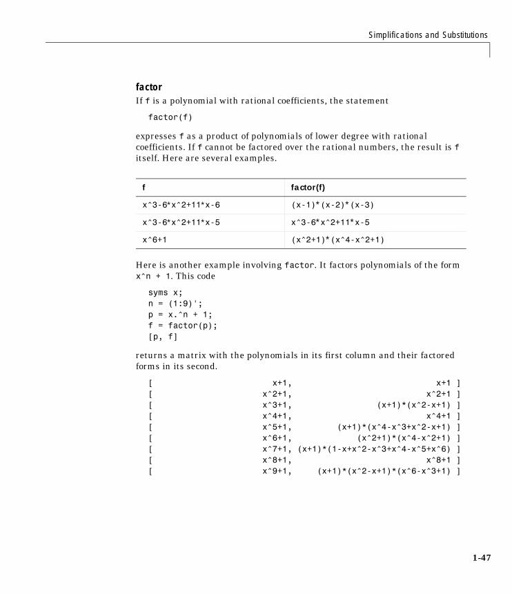
factorIf f is a polynomial with rational coefficients, the statement
factor(f)
expresses f as a product of polynomials of lower degree with rational coefficients. If f cannot be factored over the rational numbers, the result is f itself. Here are several examples.
Here is another example involving factor. It factors polynomials of the form x^n + 1. This code
syms x;n = (1:9)'; p = x.^n + 1;f = factor(p);[p, f]
returns a matrix with the polynomials in its first column and their factored forms in its second.
[ x+1, x+1 ][ x^2+1, x^2+1 ][ x^3+1, (x+1)*(x^2-x+1) ][ x^4+1, x^4+1 ][ x^5+1, (x+1)*(x^4-x^3+x^2-x+1) ][ x^6+1, (x^2+1)*(x^4-x^2+1) ][ x^7+1, (x+1)*(1-x+x^2-x^3+x^4-x^5+x^6) ][ x^8+1, x^8+1 ][ x^9+1, (x+1)*(x^2-x+1)*(x^6-x^3+1) ]
f factor(f)
x^3-6∗x^2+11∗x-6 (x-1)∗(x-2)∗(x-3)
x^3-6∗x^2+11∗x-5 x^3-6∗x^2+11∗x-5
x^6+1 (x^2+1)∗(x^4-x^2+1)
1 Using the Symbolic Math Toolbox
1-48
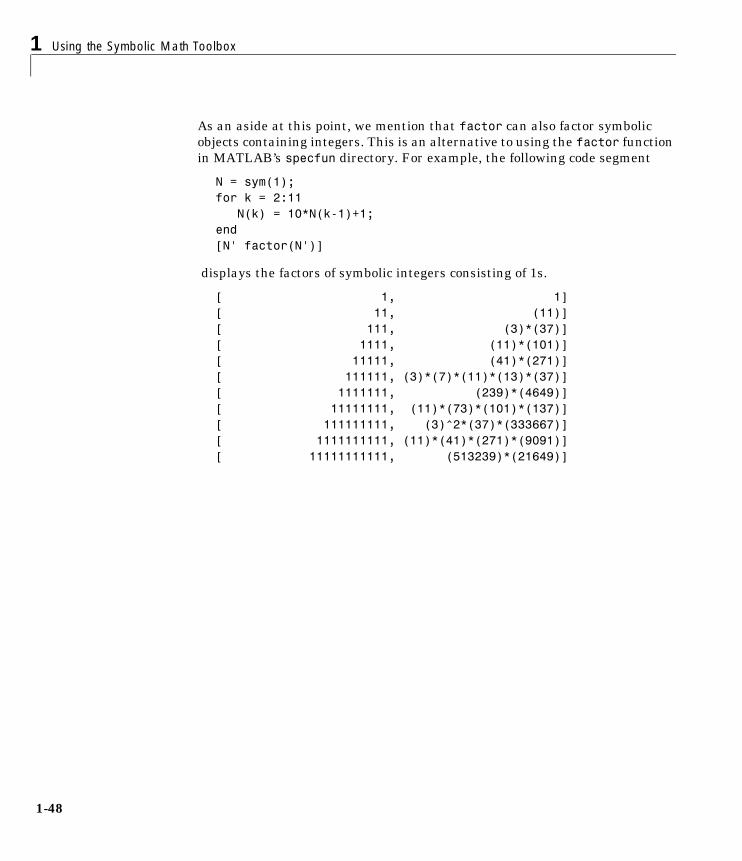
As an aside at this point, we mention that factor can also factor symbolic objects containing integers. This is an alternative to using the factor function in MATLAB’s specfun directory. For example, the following code segment
N = sym(1);for k = 2:11 N(k) = 10*N(k-1)+1;end[N' factor(N')]
displays the factors of symbolic integers consisting of 1s.
[ 1, 1][ 11, (11)][ 111, (3)*(37)][ 1111, (11)*(101)][ 11111, (41)*(271)][ 111111, (3)*(7)*(11)*(13)*(37)][ 1111111, (239)*(4649)][ 11111111, (11)*(73)*(101)*(137)][ 111111111, (3)^2*(37)*(333667)][ 1111111111, (11)*(41)*(271)*(9091)][ 11111111111, (513239)*(21649)]
Simplifications and Substitutions
1-49
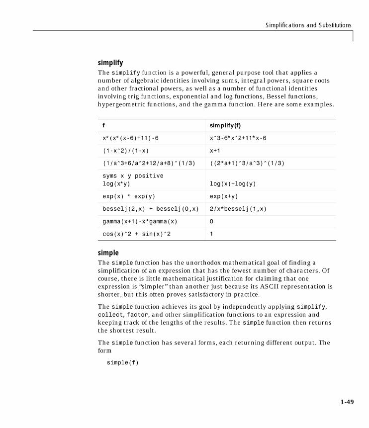
simplifyThe simplify function is a powerful, general purpose tool that applies a number of algebraic identities involving sums, integral powers, square roots and other fractional powers, as well as a number of functional identities involving trig functions, exponential and log functions, Bessel functions, hypergeometric functions, and the gamma function. Here are some examples.
simpleThe simple function has the unorthodox mathematical goal of finding a simplification of an expression that has the fewest number of characters. Of course, there is little mathematical justification for claiming that one expression is “simpler” than another just because its ASCII representation is shorter, but this often proves satisfactory in practice.
The simple function achieves its goal by independently applying simplify, collect, factor, and other simplification functions to an expression and keeping track of the lengths of the results. The simple function then returns the shortest result.
The simple function has several forms, each returning different output. The form
simple(f)
f simplify(f)
x∗(x∗(x-6)+11)-6 x^3-6∗x^2+11∗x-6
(1-x^2)/(1-x) x+1
(1/a^3+6/a^2+12/a+8)^(1/3) ((2*a+1)^3/a^3)^(1/3)
syms x y positivelog(x∗y) log(x)+log(y)
exp(x) ∗ exp(y) exp(x+y)
besselj(2,x) + besselj(0,x) 2/x*besselj(1,x)
gamma(x+1)-x*gamma(x) 0
cos(x)^2 + sin(x)^2 1

1 Using the Symbolic Math Toolbox
1-50
displays each trial simplification and the simplification function that produced it in the MATLAB command window. The simple function then returns the shortest result. For example, the command
simple(cos(x)^2 + sin(x)^2)
displays the following alternative simplifications in the MATLAB command window
simplify:1
radsimp:cos(x)^2+sin(x)^2
combine(trig):1 factor:cos(x)^2+sin(x)^2 expand:cos(x)^2+sin(x)^2 convert(exp):(1/2*exp(i*x)+1/2/exp(i*x))^2-1/4*(exp(i*x)-1/exp(i*x))^2 convert(sincos):cos(x)^2+sin(x)^2 convert(tan):(1-tan(1/2*x)^2)^2/(1+tan(1/2*x)^2)^2+4*tan(1/2*x)^2/(1+tan(1/2*x)^2)^2 collect(x):cos(x)^2+sin(x)^2
and returns
ans =1
Simplifications and Substitutions
1-51
This form is useful when you want to check, for example, whether the shortest form is indeed the simplest. If you are not interested in how simple achieves its result, use the form
f = simple(f)
This form simply returns the shortest expression found. For example, the statement
f = simple(cos(x)^2+sin(x)^2)
returns
f =1
If you want to know which simplification returned the shortest result, use the multiple output form.
[F, how] = simple(f)
This form returns the shortest result in the first variable and the simplification method used to achieve the result in the second variable. For example, the statement
[f, how] = simple(cos(x)^2+sin(x)^2)
returns
f =1 how =combine
The simple function sometimes improves on the result returned by simplify, one of the simplifications that it tries. For example, when applied to the
1 Using the Symbolic Math Toolbox
1-52
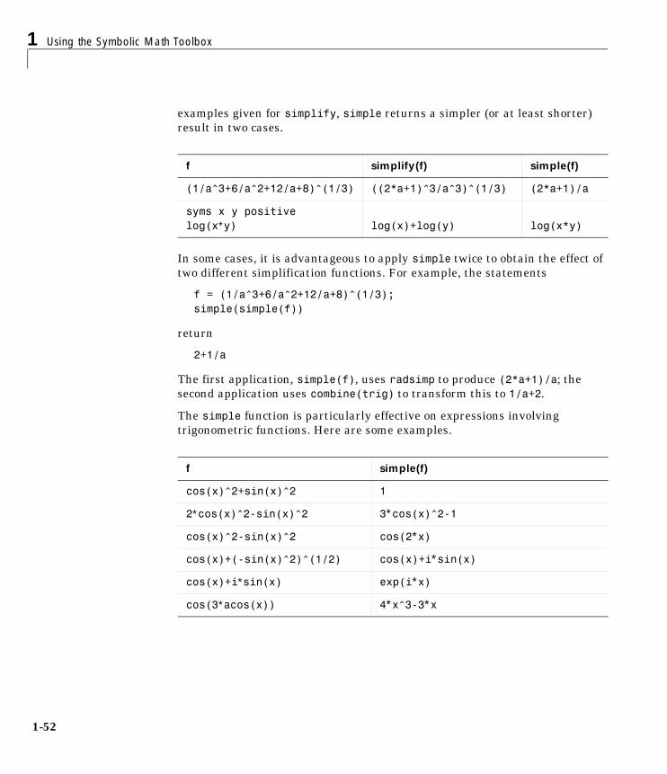
examples given for simplify, simple returns a simpler (or at least shorter) result in two cases.
In some cases, it is advantageous to apply simple twice to obtain the effect of two different simplification functions. For example, the statements
f = (1/a^3+6/a^2+12/a+8)^(1/3);simple(simple(f))
return
2+1/a
The first application, simple(f), uses radsimp to produce (2*a+1)/a; the second application uses combine(trig) to transform this to 1/a+2.
The simple function is particularly effective on expressions involving trigonometric functions. Here are some examples.
f simplify(f) simple(f)
(1/a^3+6/a^2+12/a+8)^(1/3) ((2*a+1)^3/a^3)^(1/3) (2*a+1)/a
syms x y positivelog(x∗y) log(x)+log(y) log(x*y)
f simple(f)
cos(x)^2+sin(x)^2 1
2∗cos(x)^2-sin(x)^2 3∗cos(x)^2-1
cos(x)^2-sin(x)^2 cos(2∗x)
cos(x)+(-sin(x)^2)^(1/2) cos(x)+i∗sin(x)
cos(x)+i∗sin(x) exp(i∗x)
cos(3∗acos(x)) 4∗x^3-3∗x
Simplifications and Substitutions
1-53
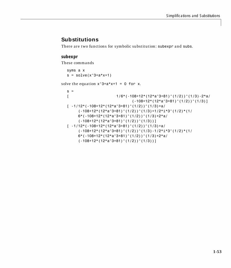
SubstitutionsThere are two functions for symbolic substitution: subexpr and subs.
subexprThese commands
syms a xs = solve(x^3+a*x+1)
solve the equation x^3+a*x+1 = 0 for x.
s =[ 1/6*(-108+12*(12*a^3+81)^(1/2))^(1/3)-2*a/ (-108+12*(12*a^3+81)^(1/2))^(1/3)][ -1/12*(-108+12*(12*a^3+81)^(1/2))^(1/3)+a/ (-108+12*(12*a^3+81)^(1/2))^(1/3)+1/2*i*3^(1/2)*(1/ 6*(-108+12*(12*a^3+81)^(1/2))^(1/3)+2*a/ (-108+12*(12*a^3+81)^(1/2))^(1/3))][ -1/12*(-108+12*(12*a^3+81)^(1/2))^(1/3)+a/ (-108+12*(12*a^3+81)^(1/2))^(1/3)-1/2*i*3^(1/2)*(1/ 6*(-108+12*(12*a^3+81)^(1/2))^(1/3)+2*a/ (-108+12*(12*a^3+81)^(1/2))^(1/3))]
1 Using the Symbolic Math Toolbox
1-54
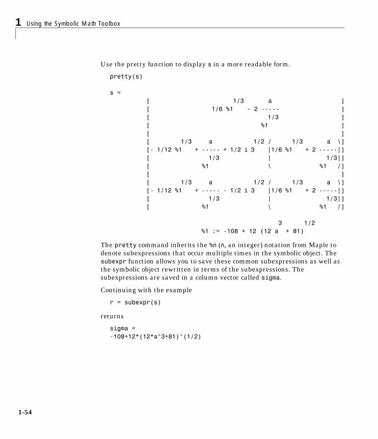
Use the pretty function to display s in a more readable form.
pretty(s) s =
[ 1/3 a ][ 1/6 %1 - 2 ----- ][ 1/3 ][ %1 ][ ][ 1/3 a 1/2 / 1/3 a \][- 1/12 %1 + ----- + 1/2 i 3 |1/6 %1 + 2 -----|][ 1/3 | 1/3|][ %1 \ %1 /][ ][ 1/3 a 1/2 / 1/3 a \][- 1/12 %1 + ----- - 1/2 i 3 |1/6 %1 + 2 -----|][ 1/3 | 1/3|][ %1 \ %1 /]
3 1/2 %1 := -108 + 12 (12 a + 81)
The pretty command inherits the %n (n, an integer) notation from Maple to denote subexpressions that occur multiple times in the symbolic object. The subexpr function allows you to save these common subexpressions as well as the symbolic object rewritten in terms of the subexpressions. The subexpressions are saved in a column vector called sigma.
Continuing with the example
r = subexpr(s)
returns
sigma =-108+12*(12*a^3+81)^(1/2)
Simplifications and Substitutions
1-55
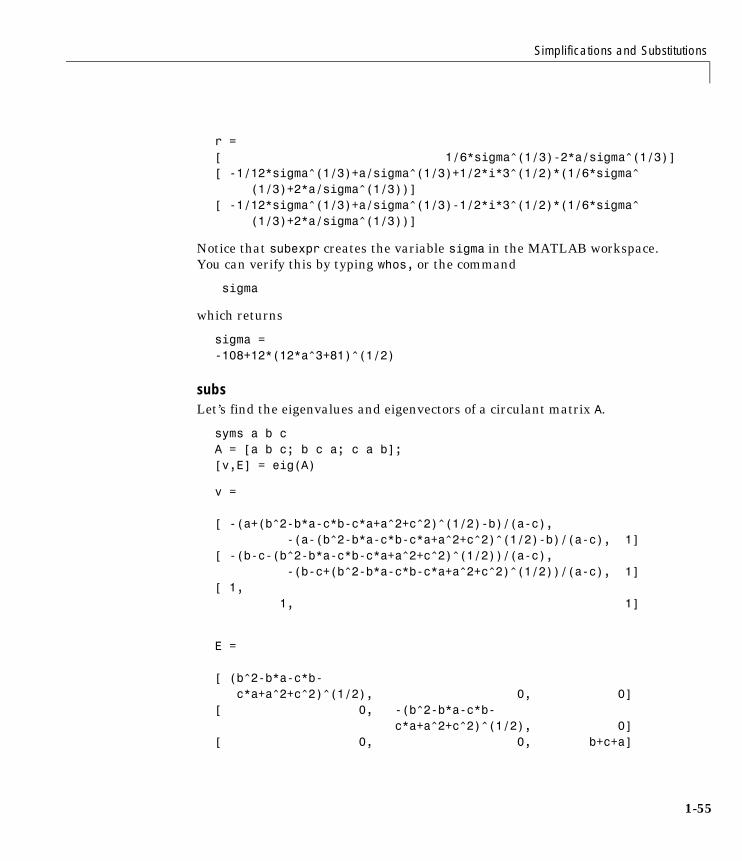
r =[ 1/6*sigma^(1/3)-2*a/sigma^(1/3)][ -1/12*sigma^(1/3)+a/sigma^(1/3)+1/2*i*3^(1/2)*(1/6*sigma^ (1/3)+2*a/sigma^(1/3))][ -1/12*sigma^(1/3)+a/sigma^(1/3)-1/2*i*3^(1/2)*(1/6*sigma^ (1/3)+2*a/sigma^(1/3))]
Notice that subexpr creates the variable sigma in the MATLAB workspace. You can verify this by typing whos, or the command
sigma
which returns
sigma =-108+12*(12*a^3+81)^(1/2)
subsLet’s find the eigenvalues and eigenvectors of a circulant matrix A.
syms a b cA = [a b c; b c a; c a b];[v,E] = eig(A)
v =
[ -(a+(b^2-b*a-c*b-c*a+a^2+c^2)^(1/2)-b)/(a-c), -(a-(b^2-b*a-c*b-c*a+a^2+c^2)^(1/2)-b)/(a-c), 1][ -(b-c-(b^2-b*a-c*b-c*a+a^2+c^2)^(1/2))/(a-c), -(b-c+(b^2-b*a-c*b-c*a+a^2+c^2)^(1/2))/(a-c), 1][ 1, 1, 1]
E =
[ (b^2-b*a-c*b- c*a+a^2+c^2)^(1/2), 0, 0][ 0, -(b^2-b*a-c*b- c*a+a^2+c^2)^(1/2), 0][ 0, 0, b+c+a]
1 Using the Symbolic Math Toolbox
1-56
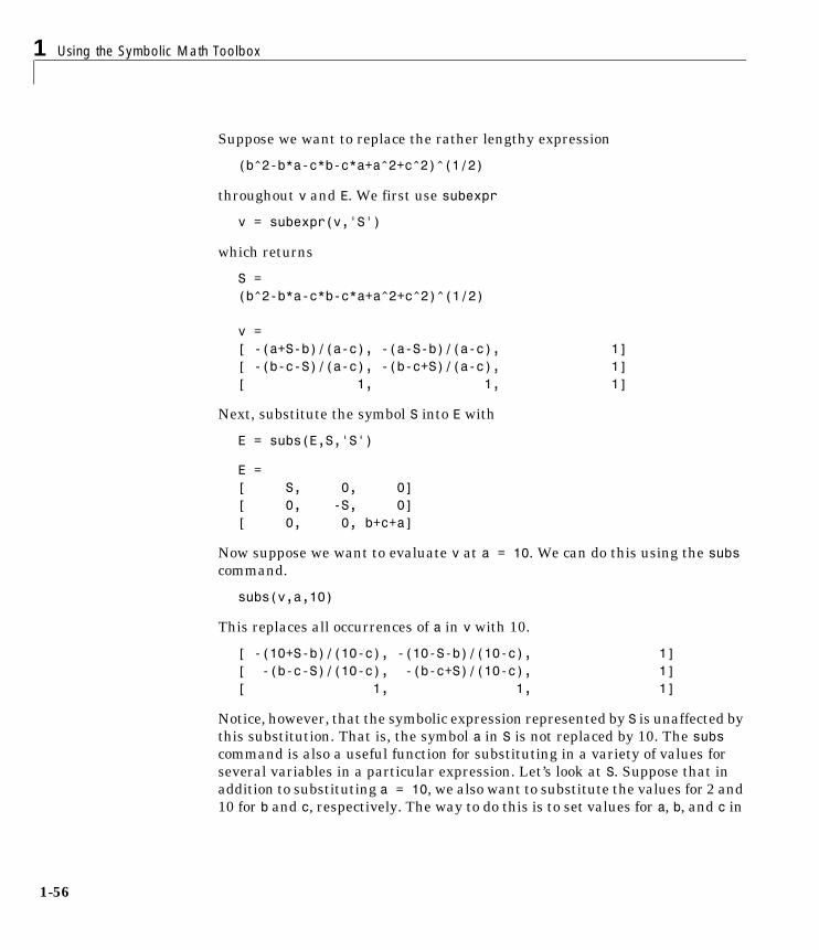
Suppose we want to replace the rather lengthy expression
(b^2-b*a-c*b-c*a+a^2+c^2)^(1/2)
throughout v and E. We first use subexpr
v = subexpr(v,'S')
which returns
S =(b^2-b*a-c*b-c*a+a^2+c^2)^(1/2)
v =[ -(a+S-b)/(a-c), -(a-S-b)/(a-c), 1][ -(b-c-S)/(a-c), -(b-c+S)/(a-c), 1][ 1, 1, 1]
Next, substitute the symbol S into E with
E = subs(E,S,'S')
E =[ S, 0, 0][ 0, -S, 0][ 0, 0, b+c+a]
Now suppose we want to evaluate v at a = 10. We can do this using the subs command.
subs(v,a,10)
This replaces all occurrences of a in v with 10.
[ -(10+S-b)/(10-c), -(10-S-b)/(10-c), 1][ -(b-c-S)/(10-c), -(b-c+S)/(10-c), 1][ 1, 1, 1]
Notice, however, that the symbolic expression represented by S is unaffected by this substitution. That is, the symbol a in S is not replaced by 10. The subs command is also a useful function for substituting in a variety of values for several variables in a particular expression. Let’s look at S. Suppose that in addition to substituting a = 10, we also want to substitute the values for 2 and 10 for b and c, respectively. The way to do this is to set values for a, b, and c in
Simplifications and Substitutions
1-57
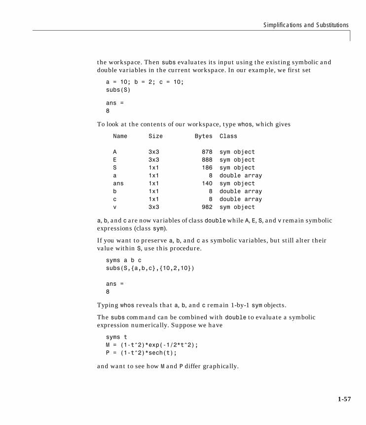
the workspace. Then subs evaluates its input using the existing symbolic and double variables in the current workspace. In our example, we first set
a = 10; b = 2; c = 10;subs(S)
ans =8
To look at the contents of our workspace, type whos, which gives
Name Size Bytes Class
A 3x3 878 sym object E 3x3 888 sym object S 1x1 186 sym object a 1x1 8 double array ans 1x1 140 sym object b 1x1 8 double array c 1x1 8 double array v 3x3 982 sym object
a, b, and c are now variables of class double while A, E, S, and v remain symbolic expressions (class sym).
If you want to preserve a, b, and c as symbolic variables, but still alter their value within S, use this procedure.
syms a b csubs(S,{a,b,c},{10,2,10})
ans =8
Typing whos reveals that a, b, and c remain 1-by-1 sym objects.
The subs command can be combined with double to evaluate a symbolic expression numerically. Suppose we have
syms tM = (1-t^2)*exp(-1/2*t^2);P = (1-t^2)*sech(t);
and want to see how M and P differ graphically.
1 Using the Symbolic Math Toolbox
1-58
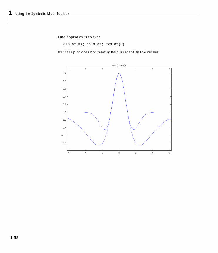
One approach is to type
ezplot(M); hold on; ezplot(P)
but this plot does not readily help us identify the curves.
−6 −4 −2 0 2 4 6
−0.8
−0.6
−0.4
−0.2
0
0.2
0.4
0.6
0.8
1
t
(1−t2) sech(t)
Simplifications and Substitutions
1-59
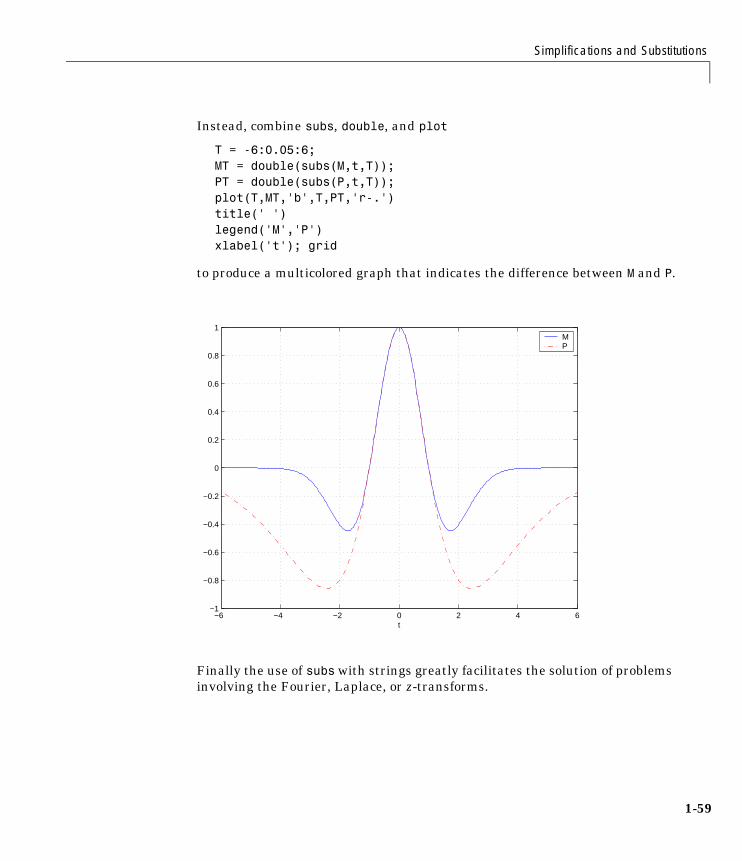
Instead, combine subs, double, and plot
T = -6:0.05:6;MT = double(subs(M,t,T));PT = double(subs(P,t,T));plot(T,MT,'b',T,PT,'r-.')title(' ')legend('M','P')xlabel('t'); grid
to produce a multicolored graph that indicates the difference between M and P.
Finally the use of subs with strings greatly facilitates the solution of problems involving the Fourier, Laplace, or z-transforms.
−6 −4 −2 0 2 4 6−1
−0.8
−0.6
−0.4
−0.2
0
0.2
0.4
0.6
0.8
1
t
MP
1 Using the Symbolic Math Toolbox
1-60
Variable-Precision Arithmetic
OverviewThere are three different kinds of arithmetic operations in this toolbox.
For example, the MATLAB statements
format long1/2+1/3
use numeric computation to produce
0.83333333333333
With the Symbolic Math Toolbox, the statement
sym(1/2)+1/3
uses symbolic computation to yield
5/6
And, also with the toolbox, the statements
digits(25)vpa('1/2+1/3')
use variable-precision arithmetic to return
.8333333333333333333333333
The floating-point operations used by numeric arithmetic are the fastest of the three, and require the least computer memory, but the results are not exact. The number of digits in the printed output of MATLAB’s double quantities is controlled by the format statement, but the internal representation is always the eight-byte floating-point representation provided by the particular computer hardware.
Numeric MATLAB’s floating-point arithmetic
Rational Maple’s exact symbolic arithmetic
VPA Maple’s variable-precision arithmetic
Variable-Precision Arithmetic
1-61
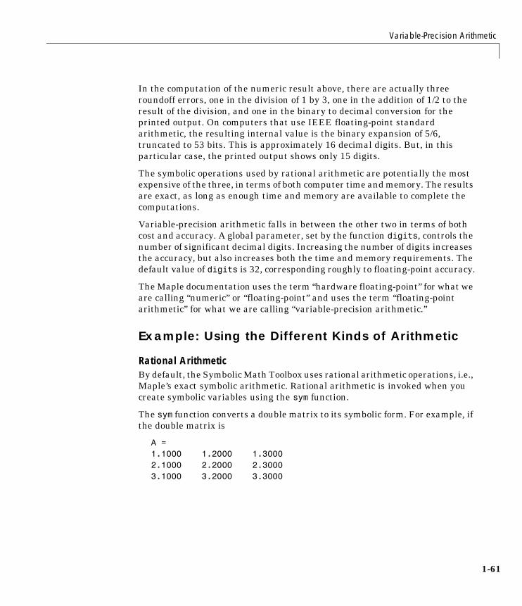
In the computation of the numeric result above, there are actually three roundoff errors, one in the division of 1 by 3, one in the addition of 1/2 to the result of the division, and one in the binary to decimal conversion for the printed output. On computers that use IEEE floating-point standard arithmetic, the resulting internal value is the binary expansion of 5/6, truncated to 53 bits. This is approximately 16 decimal digits. But, in this particular case, the printed output shows only 15 digits.
The symbolic operations used by rational arithmetic are potentially the most expensive of the three, in terms of both computer time and memory. The results are exact, as long as enough time and memory are available to complete the computations.
Variable-precision arithmetic falls in between the other two in terms of both cost and accuracy. A global parameter, set by the function digits, controls the number of significant decimal digits. Increasing the number of digits increases the accuracy, but also increases both the time and memory requirements. The default value of digits is 32, corresponding roughly to floating-point accuracy.
The Maple documentation uses the term “hardware floating-point” for what we are calling “numeric” or “floating-point” and uses the term “floating-point arithmetic” for what we are calling “variable-precision arithmetic.”
Example: Using the Different Kinds of Arithmetic
Rational ArithmeticBy default, the Symbolic Math Toolbox uses rational arithmetic operations, i.e., Maple’s exact symbolic arithmetic. Rational arithmetic is invoked when you create symbolic variables using the sym function.
The sym function converts a double matrix to its symbolic form. For example, if the double matrix is
A =1.1000 1.2000 1.30002.1000 2.2000 2.30003.1000 3.2000 3.3000

1 Using the Symbolic Math Toolbox
1-62
its symbolic form, S = sym(A), is
S =[11/10, 6/5, 13/10][21/10, 11/5, 23/10][31/10, 16/5, 33/10]
For this matrix A, it is possible to discover that the elements are the ratios of small integers, so the symbolic representation is formed from those integers. On the other hand, the statement
E = [exp(1) sqrt(2); log(3) rand]
returns a matrix
E =2.71828182845905 1.414213562373101.09861228866811 0.21895918632809
whose elements are not the ratios of small integers, so sym(E) reproduces the floating-point representation in a symbolic form.
[3060513257434037*2^(-50), 3184525836262886*2^(-51)][2473854946935174*2^(-51), 3944418039826132*2^(-54)]
Variable-Precision NumbersVariable-precision numbers are distinguished from the exact rational representation by the presence of a decimal point. A power of 10 scale factor, denoted by 'e', is allowed. To use variable-precision instead of rational arithmetic, create your variables using the vpa function.
For matrices with purely double entries, the vpa function generates the representation that is used with variable-precision arithmetic. Continuing on with our example, and using digits(4), applying vpa to the matrix S
vpa(S)
generates the output
S = [1.100, 1.200, 1.300][2.100, 2.200, 2.300][3.100, 3.200, 3.300]

Variable-Precision Arithmetic
1-63
and with digits(25)
F = vpa(E)
generates
F = [2.718281828459045534884808, 1.414213562373094923430017][1.098612288668110004152823, .2189591863280899719512718]
Converting to Floating-PointTo convert a rational or variable-precision number to its MATLAB floating-point representation, use the double function.
In our example, both double(sym(E)) and double(vpa(E)) return E.
Another ExampleThe next example is perhaps more interesting. Start with the symbolic expression
f = sym('exp(pi*sqrt(163))')
The statement
double(f)
produces the printed floating-point value
2.625374126407687e+17
Using the second argument of vpa to specify the number of digits,
vpa(f,18)
returns
262537412640768744.
whereas
vpa(f,25)
returns
262537412640768744.0000000

1 Using the Symbolic Math Toolbox
1-64
We suspect that f might actually have an integer value. This suspicion is reinforced by the 30 digit value, vpa(f,30)
262537412640768743.999999999999
Finally, the 40 digit value, vpa(f,40)
262537412640768743.9999999999992500725944
shows that f is very close to, but not exactly equal to, an integer.
Linear Algebra
1-65
Linear Algebra
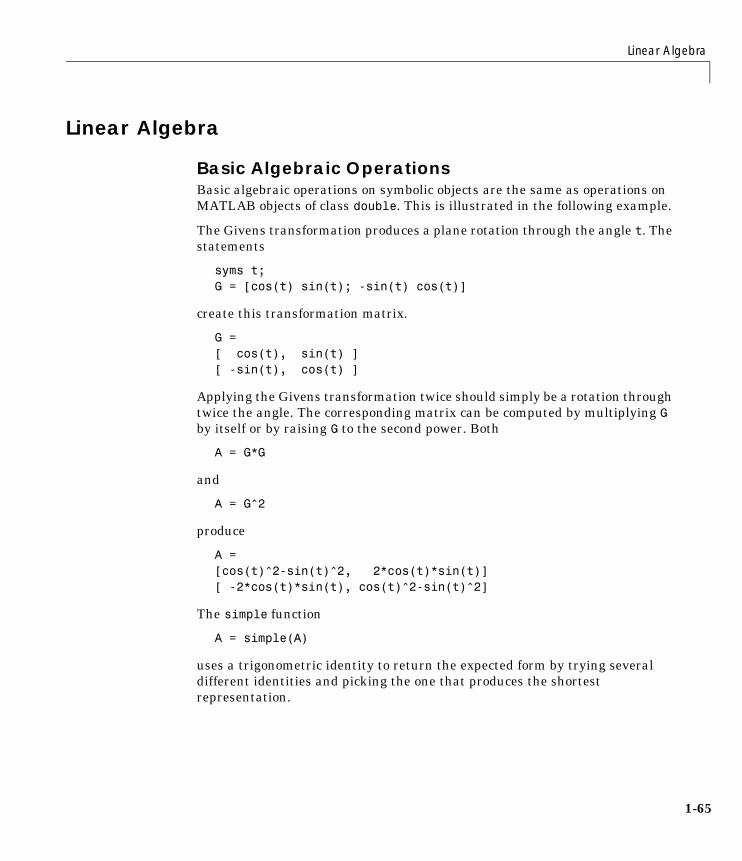
Basic Algebraic OperationsBasic algebraic operations on symbolic objects are the same as operations on MATLAB objects of class double. This is illustrated in the following example.
The Givens transformation produces a plane rotation through the angle t. The statements
syms t;G = [cos(t) sin(t); -sin(t) cos(t)]
create this transformation matrix.
G =[ cos(t), sin(t) ][ -sin(t), cos(t) ]
Applying the Givens transformation twice should simply be a rotation through twice the angle. The corresponding matrix can be computed by multiplying G by itself or by raising G to the second power. Both
A = G*G
and
A = G^2
produce
A =[cos(t)^2-sin(t)^2, 2*cos(t)*sin(t)][ -2*cos(t)*sin(t), cos(t)^2-sin(t)^2]
The simple function
A = simple(A)
uses a trigonometric identity to return the expected form by trying several different identities and picking the one that produces the shortest representation.
1 Using the Symbolic Math Toolbox
1-66
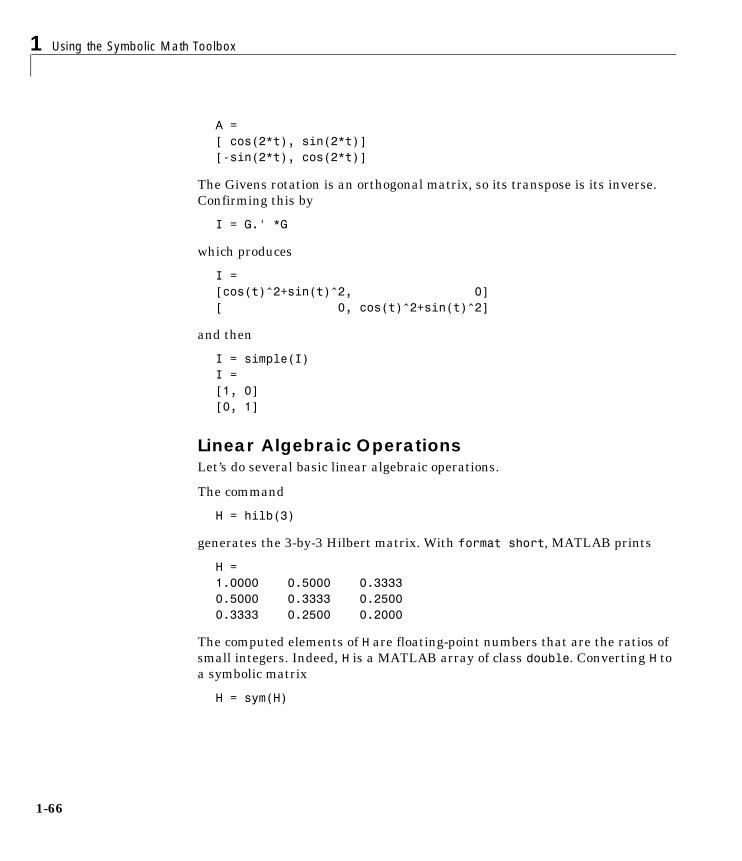
A =[ cos(2*t), sin(2*t)][-sin(2*t), cos(2*t)]
The Givens rotation is an orthogonal matrix, so its transpose is its inverse. Confirming this by
I = G.' *G
which produces
I =[cos(t)^2+sin(t)^2, 0][ 0, cos(t)^2+sin(t)^2]
and then
I = simple(I)I =[1, 0][0, 1]
Linear Algebraic OperationsLet’s do several basic linear algebraic operations.
The command
H = hilb(3)
generates the 3-by-3 Hilbert matrix. With format short, MATLAB prints
H =1.0000 0.5000 0.33330.5000 0.3333 0.25000.3333 0.2500 0.2000
The computed elements of H are floating-point numbers that are the ratios of small integers. Indeed, H is a MATLAB array of class double. Converting H to a symbolic matrix
H = sym(H)

Linear Algebra
1-67
gives
[ 1, 1/2, 1/3][1/2, 1/3, 1/4][1/3, 1/4, 1/5]
This allows subsequent symbolic operations on H to produce results that correspond to the infinitely precise Hilbert matrix, sym(hilb(3)), not its floating-point approximation, hilb(3). Therefore,
inv(H)
produces
[ 9, -36, 30][-36, 192, -180][ 30, -180, 180]
and
det(H)
yields
1/2160
We can use the backslash operator to solve a system of simultaneous linear equations. The commands
b = [1 1 1]'x = H\b % Solve Hx = b
produce the solution
[ 3][-24][ 30]
All three of these results, the inverse, the determinant, and the solution to the linear system, are the exact results corresponding to the infinitely precise, rational, Hilbert matrix. On the other hand, using digits(16), the command
V = vpa(hilb(3))

1 Using the Symbolic Math Toolbox
1-68
returns
[ 1., .5000000000000000, .3333333333333333][.5000000000000000, .3333333333333333, .2500000000000000][.3333333333333333, .2500000000000000, .2000000000000000]
The decimal points in the representation of the individual elements are the signal to use variable-precision arithmetic. The result of each arithmetic operation is rounded to 16 significant decimal digits. When inverting the matrix, these errors are magnified by the matrix condition number, which for hilb(3) is about 500. Consequently,
inv(V)
which returns
[ 9.000000000000082, -36.00000000000039, 30.00000000000035][-36.00000000000039, 192.0000000000021, -180.0000000000019][ 30.00000000000035, -180.0000000000019, 180.0000000000019]
shows the loss of two digits. So does
det(V)
which gives
.462962962962958e-3
and
V\b
which is
[ 3.000000000000041][-24.00000000000021][ 30.00000000000019]
Since H is nonsingular, the null space of H
null(H)
and the column space of H
colspace(H)

Linear Algebra
1-69
produce an empty matrix and a permutation of the identity matrix, respectively. To make a more interesting example, let’s try to find a value s for H(1,1) that makes H singular. The commands
syms sH(1,1) = sZ = det(H)sol = solve(Z)
produce
H =[ s, 1/2, 1/3][1/2, 1/3, 1/4][1/3, 1/4, 1/5]
Z =1/240*s-1/270
sol = 8/9
Then
H = subs(H,s,sol)
substitutes the computed value of sol for s in H to give
H =[8/9, 1/2, 1/3][1/2, 1/3, 1/4][1/3, 1/4, 1/5]
Now, the command
det(H)
returns
ans =0
and
inv(H)

1 Using the Symbolic Math Toolbox
1-70
produces an error message
??? error using ==> invError, (in inverse) singular matrix
because H is singular. For this matrix, Z = null(H) and C = colspace(H) are nontrivial.
Z =[ 1][ -4][10/3]
C =[ 0, 1][ 1, 0][6/5, -3/10]
It should be pointed out that even though H is singular, vpa(H) is not. For any integer value d, setting
digits(d)
and then computing
det(vpa(H))inv(vpa(H))
results in a determinant of size 10^(-d) and an inverse with elements on the order of 10^d.
EigenvaluesThe symbolic eigenvalues of a square matrix A or the symbolic eigenvalues and eigenvectors of A are computed, respectively, using the commands
E = eig(A)[V,E] = eig(A)
The variable-precision counterparts are
E = eig(vpa(A))[V,E] = eig(vpa(A))
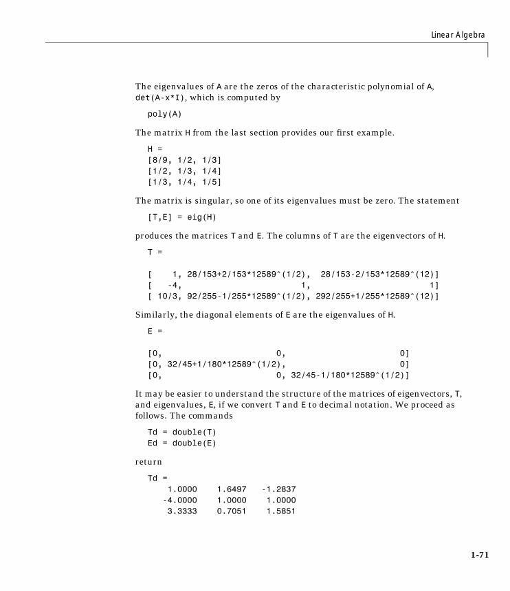
Linear Algebra
1-71
The eigenvalues of A are the zeros of the characteristic polynomial of A, det(A-x*I), which is computed by
poly(A)
The matrix H from the last section provides our first example.
H =[8/9, 1/2, 1/3][1/2, 1/3, 1/4][1/3, 1/4, 1/5]
The matrix is singular, so one of its eigenvalues must be zero. The statement
[T,E] = eig(H)
produces the matrices T and E. The columns of T are the eigenvectors of H.
T = [ 1, 28/153+2/153*12589^(1/2), 28/153-2/153*12589^(12)][ -4, 1, 1][ 10/3, 92/255-1/255*12589^(1/2), 292/255+1/255*12589^(12)]
Similarly, the diagonal elements of E are the eigenvalues of H.
E = [0, 0, 0][0, 32/45+1/180*12589^(1/2), 0][0, 0, 32/45-1/180*12589^(1/2)]
It may be easier to understand the structure of the matrices of eigenvectors, T, and eigenvalues, E, if we convert T and E to decimal notation. We proceed as follows. The commands
Td = double(T)Ed = double(E)
return
Td = 1.0000 1.6497 -1.2837 -4.0000 1.0000 1.0000 3.3333 0.7051 1.5851
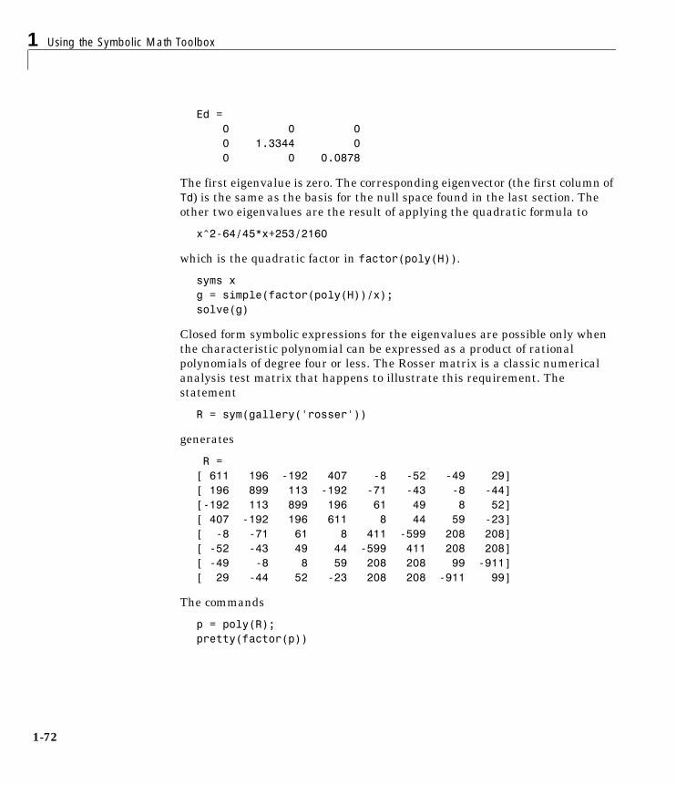
1 Using the Symbolic Math Toolbox
1-72
Ed = 0 0 0 0 1.3344 0 0 0 0.0878
The first eigenvalue is zero. The corresponding eigenvector (the first column of Td) is the same as the basis for the null space found in the last section. The other two eigenvalues are the result of applying the quadratic formula to
x^2-64/45*x+253/2160
which is the quadratic factor in factor(poly(H)).
syms xg = simple(factor(poly(H))/x);solve(g)
Closed form symbolic expressions for the eigenvalues are possible only when the characteristic polynomial can be expressed as a product of rational polynomials of degree four or less. The Rosser matrix is a classic numerical analysis test matrix that happens to illustrate this requirement. The statement
R = sym(gallery('rosser'))
generates
R = [ 611 196 -192 407 -8 -52 -49 29][ 196 899 113 -192 -71 -43 -8 -44][-192 113 899 196 61 49 8 52][ 407 -192 196 611 8 44 59 -23][ -8 -71 61 8 411 -599 208 208][ -52 -43 49 44 -599 411 208 208][ -49 -8 8 59 208 208 99 -911][ 29 -44 52 -23 208 208 -911 99]
The commands
p = poly(R);pretty(factor(p))
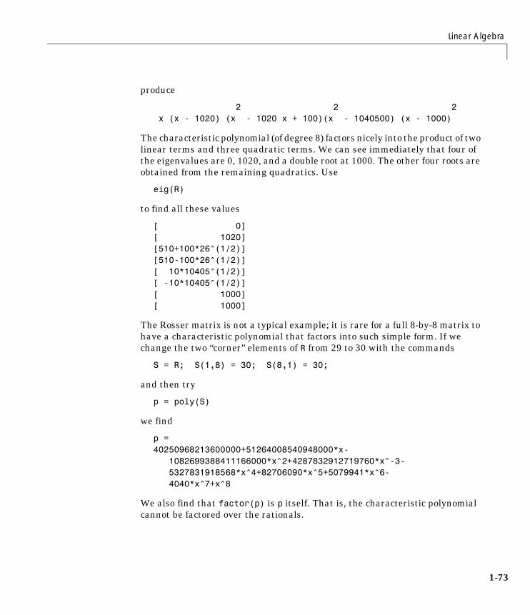
Linear Algebra
1-73
produce
2 2 2 x (x - 1020) (x - 1020 x + 100)(x - 1040500) (x - 1000)
The characteristic polynomial (of degree 8) factors nicely into the product of two linear terms and three quadratic terms. We can see immediately that four of the eigenvalues are 0, 1020, and a double root at 1000. The other four roots are obtained from the remaining quadratics. Use
eig(R)
to find all these values
[ 0][ 1020][510+100*26^(1/2)][510-100*26^(1/2)][ 10*10405^(1/2)][ -10*10405^(1/2)][ 1000][ 1000]
The Rosser matrix is not a typical example; it is rare for a full 8-by-8 matrix to have a characteristic polynomial that factors into such simple form. If we change the two “corner” elements of R from 29 to 30 with the commands
S = R; S(1,8) = 30; S(8,1) = 30;
and then try
p = poly(S)
we find
p =40250968213600000+51264008540948000*x- 1082699388411166000*x^2+4287832912719760*x^-3- 5327831918568*x^4+82706090*x^5+5079941*x^6- 4040*x^7+x^8
We also find that factor(p) is p itself. That is, the characteristic polynomial cannot be factored over the rationals.
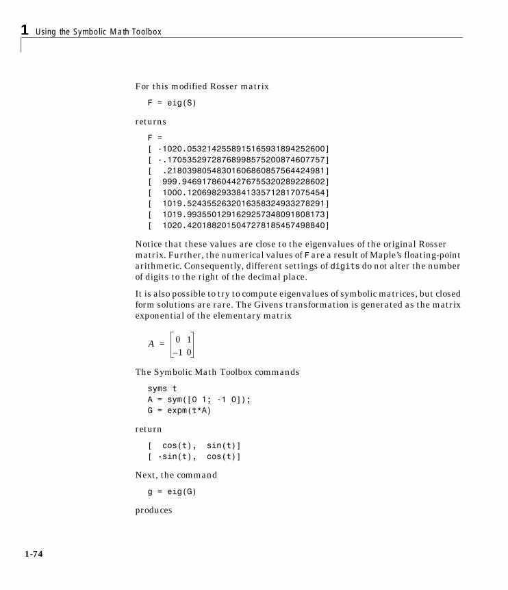
1 Using the Symbolic Math Toolbox
1-74
For this modified Rosser matrix
F = eig(S)
returns
F =[ -1020.0532142558915165931894252600][ -.17053529728768998575200874607757][ .21803980548301606860857564424981][ 999.94691786044276755320289228602][ 1000.1206982933841335712817075454][ 1019.5243552632016358324933278291][ 1019.9935501291629257348091808173][ 1020.4201882015047278185457498840]
Notice that these values are close to the eigenvalues of the original Rosser matrix. Further, the numerical values of F are a result of Maple’s floating-point arithmetic. Consequently, different settings of digits do not alter the number of digits to the right of the decimal place.
It is also possible to try to compute eigenvalues of symbolic matrices, but closed form solutions are rare. The Givens transformation is generated as the matrix exponential of the elementary matrix
The Symbolic Math Toolbox commands
syms tA = sym([0 1; -1 0]);G = expm(t*A)
return
[ cos(t), sin(t)][ -sin(t), cos(t)]
Next, the command
g = eig(G)
produces
A 0 11– 0
=

Linear Algebra
1-75
g =[ cos(t)+(cos(t)^2-1)^(1/2)][ cos(t)-(cos(t)^2-1)^(1/2)]
We can use simple to simplify this form of g. Indeed, repeated application of simple
for j = 1:4[g,how] = simple(g)
end
produces the best result
g =[ cos(t)+(-sin(t)^2)^(1/2)][ cos(t)-(-sin(t)^2)^(1/2)]
how =simplify
g =[ cos(t)+i*sin(t)][ cos(t)-i*sin(t)] how =radsimp g =[ exp(i*t)][ 1/exp(i*t)]
how =convert(exp)
g =[ exp(i*t)][ exp(-i*t)] how =combine

1 Using the Symbolic Math Toolbox
1-76
Notice the first application of simple uses simplify to produce a sum of sines and cosines. Next, simple invokes radsimp to produce cos(t) + i*sin(t) for the first eigenvector. The third application of simple uses convert(exp) to change the sines and cosines to complex exponentials. The last application of simple uses simplify to obtain the final form.
Jordan Canonical FormThe Jordan canonical form results from attempts to diagonalize a matrix by a similarity transformation. For a given matrix A, find a nonsingular matrix V, so that inv(V)*A*V, or, more succinctly, J = V\A*V, is “as close to diagonal as possible.” For almost all matrices, the Jordan canonical form is the diagonal matrix of eigenvalues and the columns of the transformation matrix are the eigenvectors. This always happens if the matrix is symmetric or if it has distinct eigenvalues. Some nonsymmetric matrices with multiple eigenvalues cannot be diagonalized. The Jordan form has the eigenvalues on its diagonal, but some of the superdiagonal elements are one, instead of zero. The statement
J = jordan(A)
computes the Jordan canonical form of A. The statement
[V,J] = jordan(A)
also computes the similarity transformation. The columns of V are the generalized eigenvectors of A.
The Jordan form is extremely sensitive to perturbations. Almost any change in A causes its Jordan form to be diagonal. This makes it very difficult to compute the Jordan form reliably with floating-point arithmetic. It also implies that A must be known exactly (i.e., without round-off error, etc.). Its elements must be integers, or ratios of small integers. In particular, the variable-precision calculation, jordan(vpa(A)), is not allowed.
For example, let
A = sym([12,32,66,116;-25,-76,-164,-294;21,66,143,256;-6,-19,-41,-73])
A =[ 12, 32, 66, 116][ -25, -76, -164, -294][ 21, 66, 143, 256][ -6, -19, -41, -73]

Linear Algebra
1-77
Then
[V,J] = jordan(A)
produces
V =[ 4, -2, 4, 3][ -6, 8, -11, -8][ 4, -7, 10, 7][ -1, 2, -3, -2]
J =[ 1, 1, 0, 0][ 0, 1, 0, 0][ 0, 0, 2, 1][ 0, 0, 0, 2]
Therefore A has a double eigenvalue at 1, with a single Jordan block, and a double eigenvalue at 2, also with a single Jordan block. The matrix has only two eigenvectors, V(:,1) and V(:,3). They satisfy
A*V(:,1) = 1*V(:,1)A*V(:,3) = 2*V(:,3)
The other two columns of V are generalized eigenvectors of grade 2. They satisfy
A*V(:,2) = 1*V(:,2) + V(:,1)A*V(:,4) = 2*V(:,4) + V(:,3)
In mathematical notation, with vj = v(:,j), the columns of V and eigenvalues satisfy the relationships
Singular Value DecompositionOnly the variable-precision numeric computation of the complete singular vector decomposition is available in the toolbox. One reason for this is that the formulas that result from symbolic computation are usually too long and
A λ2I–( )v4 v3=
A λ1I–( )v2 v1=
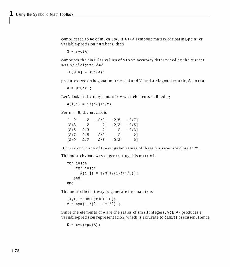
1 Using the Symbolic Math Toolbox
1-78
complicated to be of much use. If A is a symbolic matrix of floating-point or variable-precision numbers, then
S = svd(A)
computes the singular values of A to an accuracy determined by the current setting of digits. And
[U,S,V] = svd(A);
produces two orthogonal matrices, U and V, and a diagonal matrix, S, so that
A = U*S*V';
Let’s look at the n-by-n matrix A with elements defined by
A(i,j) = 1/(i-j+1/2)
For n = 5, the matrix is
[ 2 -2 -2/3 -2/5 -2/7][2/3 2 -2 -2/3 -2/5][2/5 2/3 2 -2 -2/3][2/7 2/5 2/3 2 -2][2/9 2/7 2/5 2/3 2]
It turns out many of the singular values of these matrices are close to .
The most obvious way of generating this matrix is
for i=1:n for j=1:n A(i,j) = sym(1/(i-j+1/2));
endend
The most efficient way to generate the matrix is
[J,I] = meshgrid(1:n);A = sym(1./(I - J+1/2));
Since the elements of A are the ratios of small integers, vpa(A) produces a variable-precision representation, which is accurate to digits precision. Hence
S = svd(vpa(A))
π
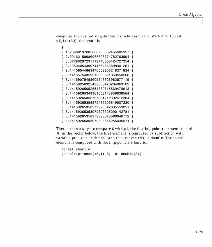
Linear Algebra
1-79
computes the desired singular values to full accuracy. With n = 16 and digits(30), the result is
S = [ 1.20968137605668985332455685357 ][ 2.69162158686066606774782763594 ][ 3.07790297231119748658424727354 ][ 3.13504054399744654843898901261 ][ 3.14106044663470063805218371924 ][ 3.14155754359918083691050658260 ][ 3.14159075458605848728982577119 ][ 3.14159256925492306470284863102 ][ 3.14159265052654880815569479613 ][ 3.14159265349961053143856838564 ][ 3.14159265358767361712392612384 ][ 3.14159265358975439206849907220 ][ 3.14159265358979270342635559051 ][ 3.14159265358979323325290142781 ][ 3.14159265358979323843066846712 ][ 3.14159265358979323846255035974 ]
There are two ways to compare S with pi, the floating-point representation of . In the vector below, the first element is computed by subtraction with
variable-precision arithmetic and then converted to a double. The second element is computed with floating-point arithmetic.
format short e[double(pi*ones(16,1)-S) pi-double(S)]
π

1 Using the Symbolic Math Toolbox
1-80
The results are
1.9319e+00 1.9319e+00 4.4997e-01 4.4997e-01 6.3690e-02 6.3690e-02 6.5521e-03 6.5521e-03 5.3221e-04 5.3221e-04 3.5110e-05 3.5110e-05 1.8990e-06 1.8990e-06 8.4335e-08 8.4335e-08 3.0632e-09 3.0632e-09 9.0183e-11 9.0183e-11 2.1196e-12 2.1196e-12 3.8846e-14 3.8636e-14 5.3504e-16 4.4409e-16 5.2097e-18 0 3.1975e-20 0 9.3024e-23 0
Since the relative accuracy of pi is pi*eps, which is 6.9757e-16, either column confirms our suspicion that four of the singular values of the 16-by-16 example equal to floating-point accuracy.
Eigenvalue TrajectoriesThis example applies several numeric, symbolic, and graphic techniques to study the behavior of matrix eigenvalues as a parameter in the matrix is varied. This particular setting involves numerical analysis and perturbation theory, but the techniques illustrated are more widely applicable.
In this example, we consider a 3-by-3 matrix A whose eigenvalues are 1, 2, 3. First, we perturb A by another matrix E and parameter . As t increases from 0 to 10-6, the eigenvalues , , change to
, , .
π
t: A A tE+→λ1 1= λ2 2= λ3 3=
λ1′ 1.5596 0.2726i+≈ λ2′ 1.5596 0.2726i–≈ λ3′ 2.8808≈

Linear Algebra
1-81
This, in turn, means that for some value of , the perturbed matrix has a double eigenvalue .
Let’s find the value of t, called , where this happens.
The starting point is a MATLAB test example, known as gallery(3).
A = gallery(3)A = -149 -50 -154 537 180 546 -27 -9 -25
This is an example of a matrix whose eigenvalues are sensitive to the effects of roundoff errors introduced during their computation. The actual computed eigenvalues may vary from one machine to another, but on a typical workstation, the statements
format long
0 0.5 1 1.5 2 2.5 3 3.5
−0.3
−0.2
−0.1
0
0.1
0.2
0.3
λ(1) λ(2) λ(3)
λ’(1)
λ’(2)
λ’(3)
t τ 0 τ 10 6–< <,=A t( ) A tE+= λ1 λ2=
τ
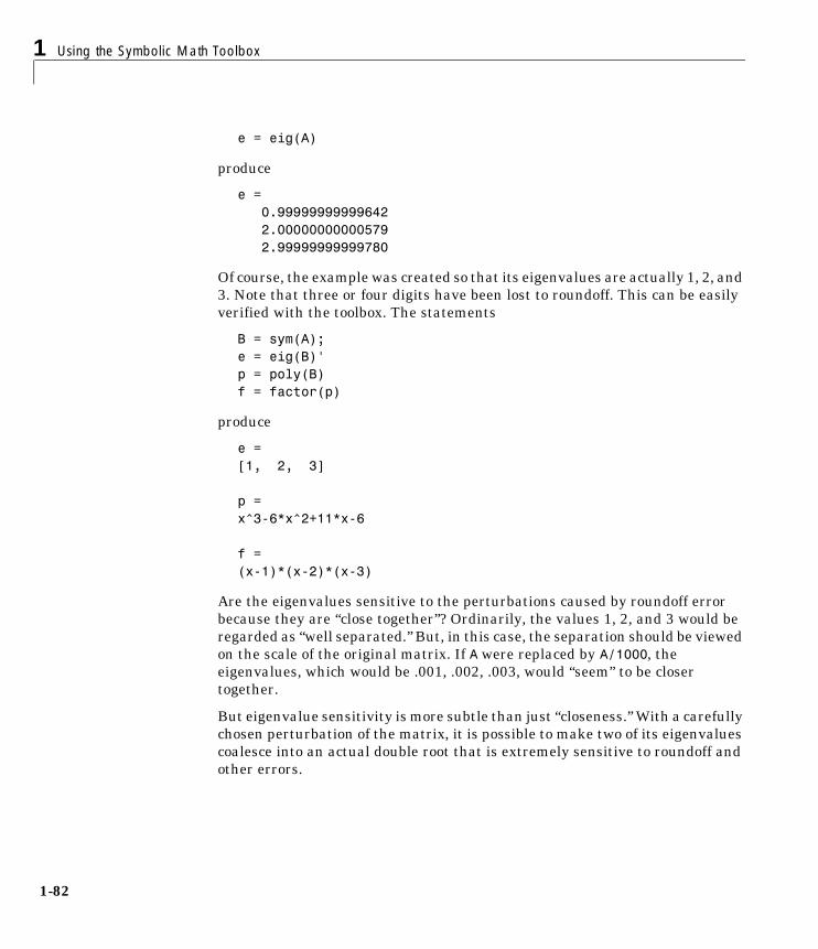
1 Using the Symbolic Math Toolbox
1-82
e = eig(A)
produce
e = 0.99999999999642 2.00000000000579 2.99999999999780
Of course, the example was created so that its eigenvalues are actually 1, 2, and 3. Note that three or four digits have been lost to roundoff. This can be easily verified with the toolbox. The statements
B = sym(A);e = eig(B)'p = poly(B)f = factor(p)
produce
e =[1, 2, 3]
p =x^3-6*x^2+11*x-6
f =(x-1)*(x-2)*(x-3)
Are the eigenvalues sensitive to the perturbations caused by roundoff error because they are “close together”? Ordinarily, the values 1, 2, and 3 would be regarded as “well separated.” But, in this case, the separation should be viewed on the scale of the original matrix. If A were replaced by A/1000, the eigenvalues, which would be .001, .002, .003, would “seem” to be closer together.
But eigenvalue sensitivity is more subtle than just “closeness.” With a carefully chosen perturbation of the matrix, it is possible to make two of its eigenvalues coalesce into an actual double root that is extremely sensitive to roundoff and other errors.
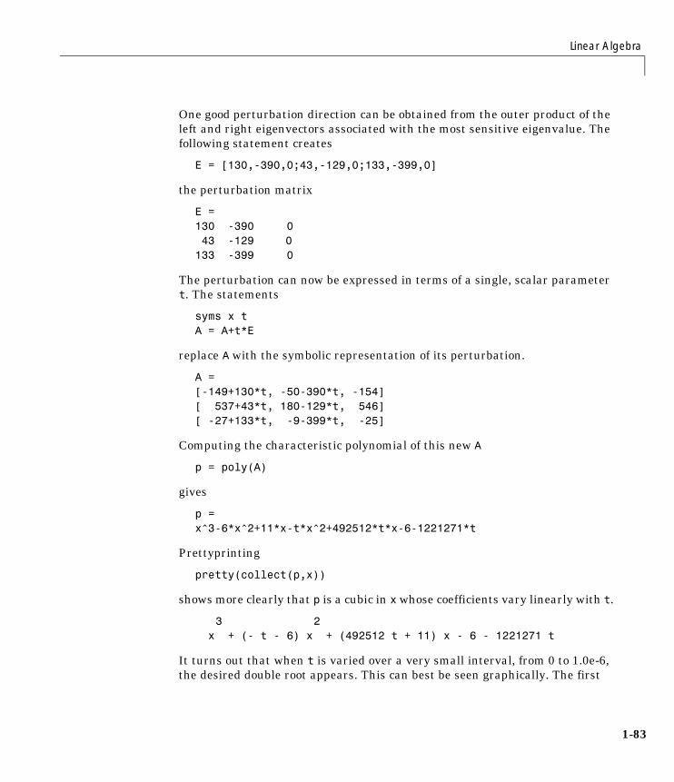
Linear Algebra
1-83
One good perturbation direction can be obtained from the outer product of the left and right eigenvectors associated with the most sensitive eigenvalue. The following statement creates
E = [130,-390,0;43,-129,0;133,-399,0]
the perturbation matrix
E =130 -390 0 43 -129 0133 -399 0
The perturbation can now be expressed in terms of a single, scalar parameter t. The statements
syms x tA = A+t*E
replace A with the symbolic representation of its perturbation.
A = [-149+130*t, -50-390*t, -154][ 537+43*t, 180-129*t, 546][ -27+133*t, -9-399*t, -25]
Computing the characteristic polynomial of this new A
p = poly(A)
gives
p =x^3-6*x^2+11*x-t*x^2+492512*t*x-6-1221271*t
Prettyprinting
pretty(collect(p,x))
shows more clearly that p is a cubic in x whose coefficients vary linearly with t.
3 2 x + (- t - 6) x + (492512 t + 11) x - 6 - 1221271 t
It turns out that when t is varied over a very small interval, from 0 to 1.0e-6, the desired double root appears. This can best be seen graphically. The first
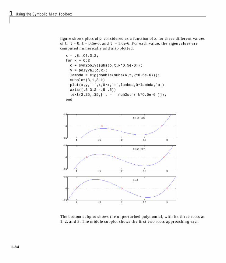
1 Using the Symbolic Math Toolbox
1-84
figure shows plots of p, considered as a function of x, for three different values of t: t = 0, t = 0.5e-6, and t = 1.0e-6. For each value, the eigenvalues are computed numerically and also plotted.
x = .8:.01:3.2; for k = 0:2c = sym2poly(subs(p,t,k*0.5e-6));y = polyval(c,x);lambda = eig(double(subs(A,t,k*0.5e-6)));subplot(3,1,3-k) plot(x,y,'-',x,0*x,':',lambda,0*lambda,'o')axis([.8 3.2 -.5 .5])text(2.25,.35,['t = ' num2str( k*0.5e-6 )]);
end
The bottom subplot shows the unperturbed polynomial, with its three roots at 1, 2, and 3. The middle subplot shows the first two roots approaching each
1 1.5 2 2.5 3−0.5
0
0.5t = 0
1 1.5 2 2.5 3−0.5
0
0.5t = 5e−007
1 1.5 2 2.5 3−0.5
0
0.5t = 1e−006
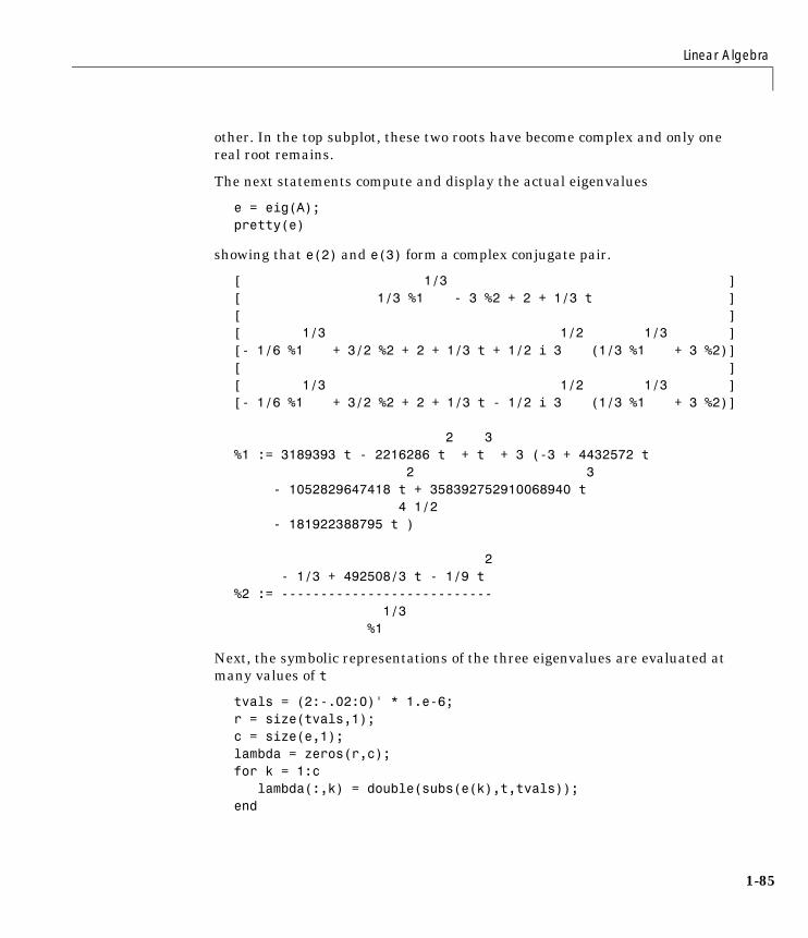
Linear Algebra
1-85
other. In the top subplot, these two roots have become complex and only one real root remains.
The next statements compute and display the actual eigenvalues
e = eig(A);pretty(e)
showing that e(2) and e(3) form a complex conjugate pair.
[ 1/3 ][ 1/3 %1 - 3 %2 + 2 + 1/3 t ][ ][ 1/3 1/2 1/3 ][- 1/6 %1 + 3/2 %2 + 2 + 1/3 t + 1/2 i 3 (1/3 %1 + 3 %2)][ ][ 1/3 1/2 1/3 ][- 1/6 %1 + 3/2 %2 + 2 + 1/3 t - 1/2 i 3 (1/3 %1 + 3 %2)] 2 3 %1 := 3189393 t - 2216286 t + t + 3 (-3 + 4432572 t 2 3 - 1052829647418 t + 358392752910068940 t 4 1/2 - 181922388795 t ) 2 - 1/3 + 492508/3 t - 1/9 t%2 := --------------------------- 1/3 %1
Next, the symbolic representations of the three eigenvalues are evaluated at many values of t
tvals = (2:-.02:0)' * 1.e-6;r = size(tvals,1);c = size(e,1);lambda = zeros(r,c);for k = 1:c
lambda(:,k) = double(subs(e(k),t,tvals));end
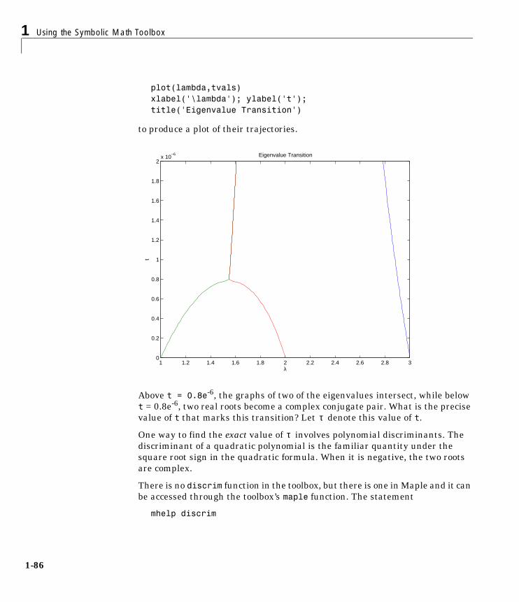
1 Using the Symbolic Math Toolbox
1-86
plot(lambda,tvals)xlabel('\lambda'); ylabel('t');title('Eigenvalue Transition')
to produce a plot of their trajectories.
Above t = 0.8e-6, the graphs of two of the eigenvalues intersect, while below t = 0.8e-6, two real roots become a complex conjugate pair. What is the precise value of t that marks this transition? Let denote this value of t.
One way to find the exact value of involves polynomial discriminants. The discriminant of a quadratic polynomial is the familiar quantity under the square root sign in the quadratic formula. When it is negative, the two roots are complex.
There is no discrim function in the toolbox, but there is one in Maple and it can be accessed through the toolbox’s maple function. The statement
mhelp discrim
1 1.2 1.4 1.6 1.8 2 2.2 2.4 2.6 2.8 30
0.2
0.4
0.6
0.8
1
1.2
1.4
1.6
1.8
2x 10
−6
λ
t
Eigenvalue Transition
τ
τ

Linear Algebra
1-87
provides a brief explanation. Use these commands
syms a b c xmaple('discrim', a*x^2+b*x+c, x)
to show the generic quadratic’s discriminant, b2 - 4ac
ans =-4*a*c+b^2
The discriminant for the perturbed cubic characteristic polynomial is obtained, using
discrim = maple('discrim',p,x)
which produces
[discrim =4-5910096*t+1403772863224*t^2-477857003880091920*t^3+242563185060*t^4]
The quantity is one of the four roots of this quartic. Let’s find a numeric value for .
digits(24) s = solve(discrim);tau = vpa(s)
tau =[ 1970031.04061804553618913][ .783792490602e-6][ .1076924816049e-5+.318896441018863170083895e-5*i][ .1076924816049e-5-.318896441018863170083895e-5*i]
Of the four solutions, we know that
tau = tau(2)
is the transition point
tau =.783792490602e-6
because it is closest to our previous estimate.
ττ
1 Using the Symbolic Math Toolbox
1-88
A more generally applicable method for finding is based on the fact that, at a double root, both the function and its derivative must vanish. This results in two polynomial equations to be solved for two unknowns. The statement
sol = solve(p,diff(p,'x'))
solves the pair of algebraic equations p = 0 and dp/dx = 0 and produces
sol = t: [4x1 sym] x: [4x1 sym]
Find now by
tau = double(sol.t(2))
which reveals that the second element of sol.t is the desired value of .
format shorttau =
7.8379e-07
Therefore, the second element of sol.x
sigma = double(sol.x(2))
is the double eigenvalue
sigma =1.5476
Let’s verify that this value of does indeed produce a double eigenvalue at . To achieve this, substitute for t in the perturbed matrix
and find the eigenvalues of . That is,
e = eig(double(subs(A,t,tau)))
e = 1.5476 1.5476 2.9047
confirms that is a double eigenvalue of for t = 7.8379e-07.
τ
τ
τ
τσ 1.5476= τA t( ) A tE+= A t( )
σ 1.5476= A t( )
Solving Equations
1-89
Solving Equations
Solving Algebraic EquationsIf S is a symbolic expression,
solve(S)
attempts to find values of the symbolic variable in S (as determined by findsym) for which S is zero. For example,
syms a b c xS = a*x^2 + b*x + c;solve(S)
uses the familiar quadratic formula to produce
ans =[1/2/a*(-b+(b^2-4*a*c)^(1/2))][1/2/a*(-b-(b^2-4*a*c)^(1/2))]
This is a symbolic vector whose elements are the two solutions.
If you want to solve for a specific variable, you must specify that variable as an additional argument. For example, if you want to solve S for b, use the command
b = solve(S,b)
which returns
b =-(a*x^2+c)/x
Note that these examples assume equations of the form . If you need to solve equations of the form , you must use quoted strings. In particular, the command
s = solve('cos(2*x)+sin(x)=1')
returns a vector with four solutions.
f x( ) 0=f x( ) q x( )=
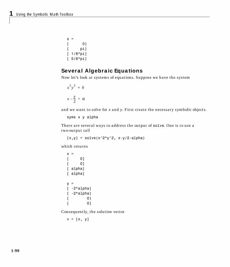
1 Using the Symbolic Math Toolbox
1-90
s =[ 0][ pi][ 1/6*pi][ 5/6*pi]
Several Algebraic EquationsNow let’s look at systems of equations. Suppose we have the system
and we want to solve for x and y. First create the necessary symbolic objects.
syms x y alpha
There are several ways to address the output of solve. One is to use a two-output call
[x,y] = solve(x^2*y^2, x-y/2-alpha)
which returns
x = [ 0][ 0][ alpha][ alpha]
y = [ -2*alpha][ -2*alpha][ 0][ 0]
Consequently, the solution vector
v = [x, y]
x2y2 0=
x y2---– α=

Solving Equations
1-91
appears to have redundant components. This is due to the first equation , which has two solutions in x and y: , . Changing the
equations to
eqs1 = 'x^2*y^2=1, x-y/2-alpha'[x,y] = solve(eqs1)
produces four distinct solutions.
x =[ 1/2*alpha+1/2*(alpha^2+2)^(1/2)][ 1/2*alpha-1/2*(alpha^2+2)^(1/2)][ 1/2*alpha+1/2*(alpha^2-2)^(1/2)][ 1/2*alpha-1/2*(alpha^2-2)^(1/2)] y =[ -alpha+(alpha^2+2)^(1/2)][ -alpha-(alpha^2+2)^(1/2)][ -alpha+(alpha^2-2)^(1/2)][ -alpha-(alpha^2-2)^(1/2)]
Since we did not specify the dependent variables, solve uses findsym to determine the variables.
This way of assigning output from solve is quite successful for “small” systems. Plainly, if we had, say, a 10-by-10 system of equations, typing
[x1,x2,x3,x4,x5,x6,x7,x8,x9,x10] = solve(...)
is both awkward and time consuming. To circumvent this difficulty, solve can return a structure whose fields are the solutions. In particular, consider the system u^2-v^2 = a^2, u + v = 1, a^2-2*a = 3. The command
S = solve('u^2-v^2 = a^2','u + v = 1','a^2-2*a = 3')
returns
S = a: [2x1 sym] u: [2x1 sym] v: [2x1 sym]
The solutions for a reside in the “a-field” of S. That is,
x2y2 0= x 0±= y 0±=
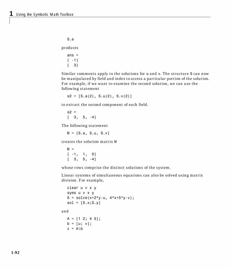
1 Using the Symbolic Math Toolbox
1-92
S.a
produces
ans =[ -1][ 3]
Similar comments apply to the solutions for u and v. The structure S can now be manipulated by field and index to access a particular portion of the solution. For example, if we want to examine the second solution, we can use the following statement
s2 = [S.a(2), S.u(2), S.v(2)]
to extract the second component of each field.
s2 =[ 3, 5, -4]
The following statement
M = [S.a, S.u, S.v]
creates the solution matrix M
M = [ -1, 1, 0][ 3, 5, -4]
whose rows comprise the distinct solutions of the system.
Linear systems of simultaneous equations can also be solved using matrix division. For example,
clear u v x ysyms u v x yS = solve(x+2*y-u, 4*x+5*y-v);sol = [S.x;S.y]
and
A = [1 2; 4 5];b = [u; v];z = A\b

Solving Equations
1-93
result in
sol = [ -5/3*u+2/3*v][ 4/3*u-1/3*v]
z =[ -5/3*u+2/3*v][ 4/3*u-1/3*v]
Thus s and z produce the same solution, although the results are assigned to different variables.
Single Differential EquationThe function dsolve computes symbolic solutions to ordinary differential equations. The equations are specified by symbolic expressions containing the letter D to denote differentiation. The symbols D2, D3, ... DN, correspond to the second, third, ..., Nth derivative, respectively. Thus, D2y is the Symbolic Math Toolbox equivalent of . The dependent variables are those preceded by D and the default independent variable is t. Note that names of symbolic variables should not contain D. The independent variable can be changed from t to some other symbolic variable by including that variable as the last input argument.
Initial conditions can be specified by additional equations. If initial conditions are not specified, the solutions contain constants of integration, C1, C2, etc.
The output from dsolve parallels the output from solve. That is, you can call dsolve with the number of output variables equal to the number of dependent variables or place the output in a structure whose fields contain the solutions of the differential equations.
Example 1The following call to dsolve
dsolve('Dy=1+y^2')
uses y as the dependent variable and t as the default independent variable. The output of this command is
d2y dt2⁄
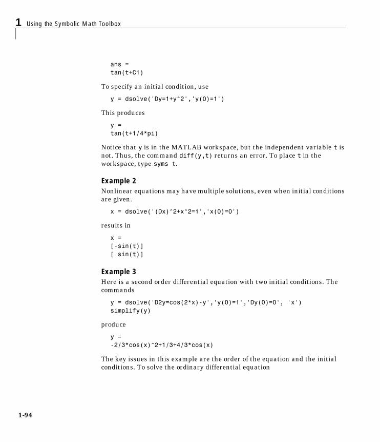
1 Using the Symbolic Math Toolbox
1-94
ans = tan(t+C1)
To specify an initial condition, use
y = dsolve('Dy=1+y^2','y(0)=1')
This produces
y =tan(t+1/4*pi)
Notice that y is in the MATLAB workspace, but the independent variable t is not. Thus, the command diff(y,t) returns an error. To place t in the workspace, type syms t.
Example 2Nonlinear equations may have multiple solutions, even when initial conditions are given.
x = dsolve('(Dx)^2+x^2=1','x(0)=0')
results in
x =[-sin(t)][ sin(t)]
Example 3Here is a second order differential equation with two initial conditions. The commands
y = dsolve('D2y=cos(2*x)-y','y(0)=1','Dy(0)=0', 'x')simplify(y)
produce
y =-2/3*cos(x)^2+1/3+4/3*cos(x)
The key issues in this example are the order of the equation and the initial conditions. To solve the ordinary differential equation
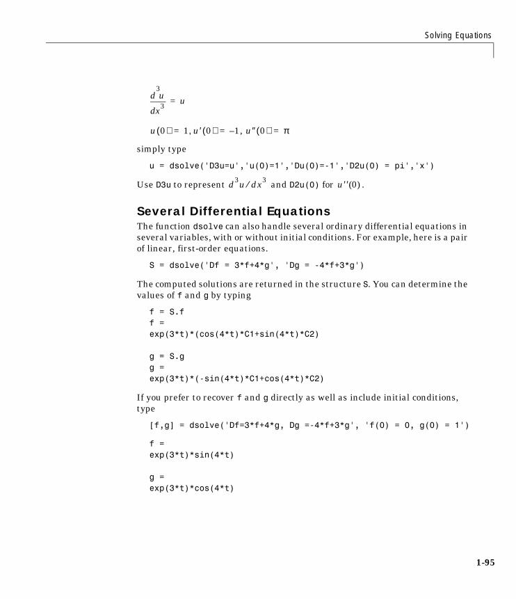
Solving Equations
1-95
simply type
u = dsolve('D3u=u','u(0)=1','Du(0)=-1','D2u(0) = pi','x')
Use D3u to represent and D2u(0) for .
Several Differential EquationsThe function dsolve can also handle several ordinary differential equations in several variables, with or without initial conditions. For example, here is a pair of linear, first-order equations.
S = dsolve('Df = 3*f+4*g', 'Dg = -4*f+3*g')
The computed solutions are returned in the structure S. You can determine the values of f and g by typing
f = S.ff = exp(3*t)*(cos(4*t)*C1+sin(4*t)*C2)
g = S.gg =exp(3*t)*(-sin(4*t)*C1+cos(4*t)*C2)
If you prefer to recover f and g directly as well as include initial conditions, type
[f,g] = dsolve('Df=3*f+4*g, Dg =-4*f+3*g', 'f(0) = 0, g(0) = 1')
f =exp(3*t)*sin(4*t)
g =exp(3*t)*cos(4*t)
x3
3
d
d u u=
u 0( ) 1 u′ 0( ), 1, u″ 0( )– π= = =
d3u dx3⁄ u′′ 0( )
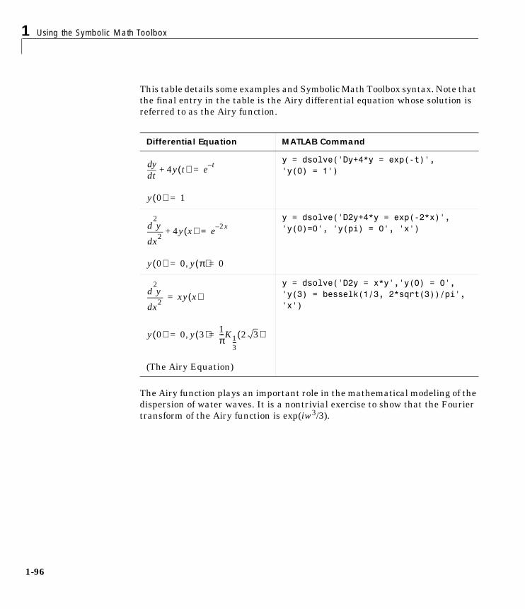
1 Using the Symbolic Math Toolbox
1-96
This table details some examples and Symbolic Math Toolbox syntax. Note that the final entry in the table is the Airy differential equation whose solution is referred to as the Airy function.
The Airy function plays an important role in the mathematical modeling of the dispersion of water waves. It is a nontrivial exercise to show that the Fourier transform of the Airy function is exp(iw3/3).
Differential Equation MATLAB Command
y = dsolve('Dy+4*y = exp(-t)', 'y(0) = 1')
y = dsolve('D2y+4*y = exp(-2*x)', 'y(0)=0', 'y(pi) = 0', 'x')
(The Airy Equation)
y = dsolve('D2y = x*y','y(0) = 0', 'y(3) = besselk(1/3, 2*sqrt(3))/pi', 'x')
tddy 4y t( )+ e t–
=
y 0( ) 1=
x2
2
d
d y 4y x( )+ e 2x–=
y 0( ) 0 y π( ) 0=,=
x2
2
d
d y xy x( )=
y 0( ) 0 y 3( ) 1π---K1
3---
2 3( )=,=
Special Mathematical Functions
1-97
Special Mathematical FunctionsOver fifty of the special functions of classical applied mathematics are available in the toolbox. These functions are accessed with the mfun function, which numerically evaluates a special function for the specified parameters. This allows you to evaluate functions that are not available in standard MATLAB, such as the Fresnel cosine integral. In addition, you can evaluate several MATLAB special functions in the complex plane, such as the error function.
For example, suppose you want to evaluate the hyperbolic cosine integral at the points 2+i, 0, and 4.5. First type
help mfunlist
to see the list of functions available for mfun. This list provides a brief mathematical description of each function, its Maple name, and the parameters it needs. From the list, you can see that the hyperbolic cosine integral is called Chi, and it takes one complex argument. For additional information, you can access Maple help on the hyperbolic cosine integral using
mhelp Chi
Now type
z = [2+i 0 4.5];w = mfun('Chi',z)
which returns
w = 2.0303 + 1.7227i NaN 13.9658
mfun returns NaNs where the function has a singularity. The hyperbolic cosine integral has a singularity at z = 0.
These special functions can be used with the mfun function:
• Airy Functions
• Binomial Coefficients
• Riemann Zeta Functions
• Bernoulli Numbers and Polynomials
• Euler Numbers and Polynomials
1 Using the Symbolic Math Toolbox
1-98
• Harmonic Function
• Exponential Integrals
• Logarithmic Integral
• Sine and Cosine Integrals
• Hyperbolic Sine and Cosine Integrals
• Shifted Sine Integral
• Fresnel Sine and Cosine Integral
• Dawson’s Integral
• Error Function
• Complementary Error Function and its Iterated Integrals
• Gamma Function
• Logarithm of the Gamma Function
• Incomplete Gamma Function
• Digamma Function
• Polygamma Function
• Generalized Hypergeometric Function
• Bessel Functions
• Incomplete Elliptic Integrals
• Complete Elliptic Integrals
• Complete Elliptic Integrals with Complementary Modulus
• Beta Function
• Dilogarithm Integral
• Lambert’s W Function
• Dirac Delta Function (distribution)
• Heaviside Function (distribution)
The orthogonal polynomials listed below are available with the Extended Symbolic Math Toolbox:
• Gegenbauer
• Hermite
• Laguerre

Special Mathematical Functions
1-99
• Generalized Laguerre
• Legendre
• Jacobi
• Chebyshev of the First and Second Kind
DiffractionThis example is from diffraction theory in classical electrodynamics. (J.D. Jackson, Classical Electrodynamics, John Wiley & Sons, 1962.)
Suppose we have a plane wave of intensity I0 and wave number k. We assume that the plane wave is parallel to the xy-plane and travels along the z-axis as shown below. This plane wave is called the incident wave. A perfectly conducting flat diffraction screen occupies half of the xy-plane, that is x < 0. The plane wave strikes the diffraction screen, and we observe the diffracted wave from the line whose coordinates are (x, 0, z0), where z0 > 0.
The intensity of the diffracted wave is given by
where
diffraction screen
x
zy
line of observation
(x0,0,z0)
incident plane wave
II02----- C ζ( ) 1
2---+
2S ζ( ) 1
2---+
2+=
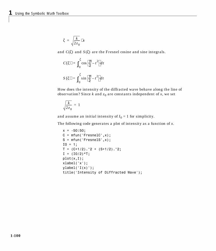
1 Using the Symbolic Math Toolbox
1-100
and and are the Fresnel cosine and sine integrals.
How does the intensity of the diffracted wave behave along the line of observation? Since k and z0 are constants independent of x, we set
and assume an initial intensity of I0 = 1 for simplicity.
The following code generates a plot of intensity as a function of x.
x = -50:50;C = mfun('FresnelC',x);S = mfun('FresnelS',x);I0 = 1;T = (C+1/2).^2 + (S+1/2).^2;I = (I0/2)*T;plot(x,I);xlabel('x');ylabel('I(x)');title('Intensity of Diffracted Wave');
ζ k2z0--------- x⋅=
C ζ( ) S ζ( )
C ζ( ) π2--- t2
– tdcos
0
ζ
∫=
S ζ( ) π2--- t2
– sin td
0
ζ
∫=
k2z0--------- 1=
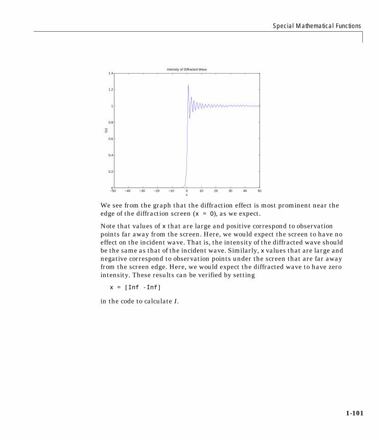
Special Mathematical Functions
1-101
We see from the graph that the diffraction effect is most prominent near the edge of the diffraction screen (x = 0), as we expect.
Note that values of x that are large and positive correspond to observation points far away from the screen. Here, we would expect the screen to have no effect on the incident wave. That is, the intensity of the diffracted wave should be the same as that of the incident wave. Similarly, x values that are large and negative correspond to observation points under the screen that are far away from the screen edge. Here, we would expect the diffracted wave to have zero intensity. These results can be verified by setting
x = [Inf -Inf]
in the code to calculate I.
−50 −40 −30 −20 −10 0 10 20 30 40 500
0.2
0.4
0.6
0.8
1
1.2
1.4
x
I(x)
Intensity of Diffracted Wave
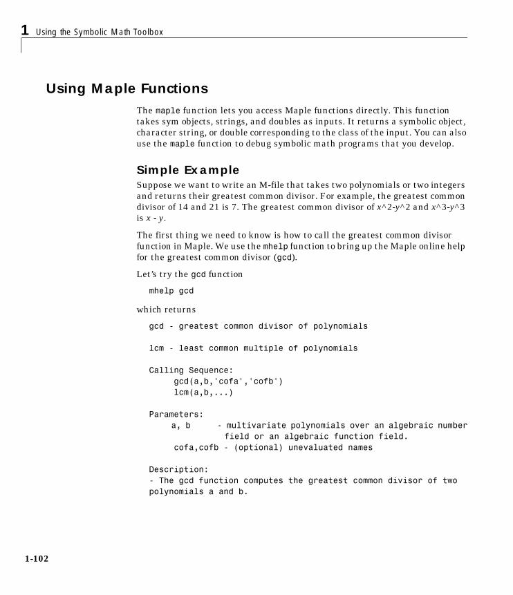
1 Using the Symbolic Math Toolbox
1-102
Using Maple FunctionsThe maple function lets you access Maple functions directly. This function takes sym objects, strings, and doubles as inputs. It returns a symbolic object, character string, or double corresponding to the class of the input. You can also use the maple function to debug symbolic math programs that you develop.
Simple ExampleSuppose we want to write an M-file that takes two polynomials or two integers and returns their greatest common divisor. For example, the greatest common divisor of 14 and 21 is 7. The greatest common divisor of x^2-y^2 and x^3-y^3 is x - y.
The first thing we need to know is how to call the greatest common divisor function in Maple. We use the mhelp function to bring up the Maple online help for the greatest common divisor (gcd).
Let’s try the gcd function
mhelp gcd
which returns
gcd - greatest common divisor of polynomials
lcm - least common multiple of polynomials
Calling Sequence: gcd(a,b,'cofa','cofb') lcm(a,b,...)
Parameters: a, b - multivariate polynomials over an algebraic number
field or an algebraic function field. cofa,cofb - (optional) unevaluated names
Description:- The gcd function computes the greatest common divisor of two polynomials a and b.
Using Maple Functions
1-103
- If the coefficients of a and b are integers, then, a primitive unit normal greatest common divisor is returned. In other words, the coefficients of the result are relatively prime integers and the leading coefficient is a positive integer.
- If the coefficients of a or b are rational numbers or belong to an algebraic number or function field, then the monic greatest common divisor of a and b is computed. See type,algnum and type,algfun.
- Algebraic numbers and functions may be represented by radicals (see type,radical) or with the RootOf notation (see evala).
- Names occurring inside a RootOf or a radical are viewed as elements of the coefficient field, provided the RootOf defines an algebraic function. Therefore, they may occur in denominators as well. Other names are not allowed in denominators.
- If a or b contains objects that are not algebraic numbers nor algebraic functions, these objects will be frozen before the computation proceeds. See frontend.
- The RootOf and the radicals defining the algebraic numbers must form an independent set of algebraic quantities, otherwise an error is returned. Note that this condition needs not be satisfied if the expression contains only algebraic numbers in radical notation (i.e. 2^(1/2), 3^(1/2), 6^(1/2)). For, a basis over Q for the radicals can be computed by Maple in this case.
- Since the ordering of the variables depends on the session, the result may also depend on the session when a and b have several variables.
- The lcm function computes the least common multiple of an arbitrary number of polynomials.
- The optional third argument cofa is assigned the cofactor a/gcd(a,b).
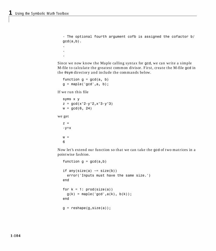
1 Using the Symbolic Math Toolbox
1-104
- The optional fourth argument cofb is assigned the cofactor b/gcd(a,b). ...
Since we now know the Maple calling syntax for gcd, we can write a simple M-file to calculate the greatest common divisor. First, create the M-file gcd in the @sym directory and include the commands below.
function g = gcd(a, b)g = maple('gcd',a, b);
If we run this file
syms x yz = gcd(x^2-y^2,x^3-y^3)w = gcd(6, 24)
we get
z = -y+x
w = 6
Now let’s extend our function so that we can take the gcd of two matrices in a pointwise fashion.
function g = gcd(a,b)
if any(size(a) ~= size(b)) error('Inputs must have the same size.')end
for k = 1: prod(size(a)) g(k) = maple('gcd',a(k), b(k));end
g = reshape(g,size(a));
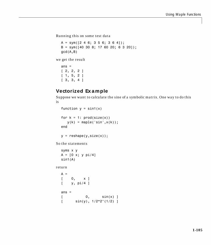
Using Maple Functions
1-105
Running this on some test data
A = sym([2 4 6; 3 5 6; 3 6 4]);B = sym([40 30 8; 17 60 20; 6 3 20]);gcd(A,B)
we get the result
ans =[ 2, 2, 2 ][ 1, 5, 2 ][ 3, 3, 4 ]
Vectorized ExampleSuppose we want to calculate the sine of a symbolic matrix. One way to do this is
function y = sin1(x)
for k = 1: prod(size(x)) y(k) = maple('sin',x(k));end
y = reshape(y,size(x));
So the statements
syms x yA = [0 x; y pi/4]sin1(A)
return
A =[ 0, x ][ y, pi/4 ] ans =[ 0, sin(x) ][ sin(y), 1/2*2^(1/2) ]
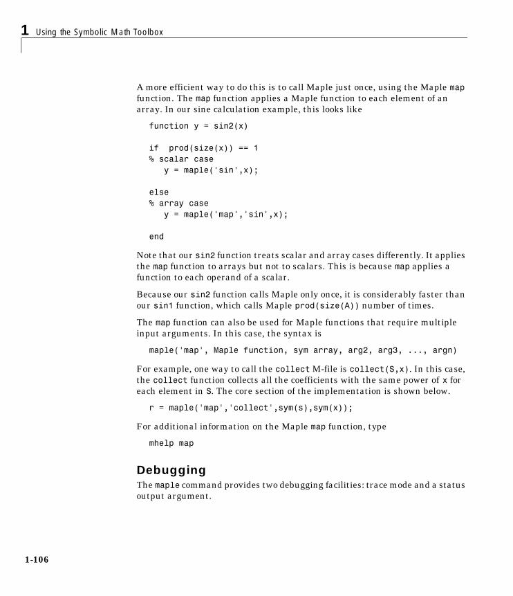
1 Using the Symbolic Math Toolbox
1-106
A more efficient way to do this is to call Maple just once, using the Maple map function. The map function applies a Maple function to each element of an array. In our sine calculation example, this looks like
function y = sin2(x)
if prod(size(x)) == 1% scalar case y = maple('sin',x);
else% array case y = maple('map','sin',x);
end
Note that our sin2 function treats scalar and array cases differently. It applies the map function to arrays but not to scalars. This is because map applies a function to each operand of a scalar.
Because our sin2 function calls Maple only once, it is considerably faster than our sin1 function, which calls Maple prod(size(A)) number of times.
The map function can also be used for Maple functions that require multiple input arguments. In this case, the syntax is
maple('map', Maple function, sym array, arg2, arg3, ..., argn)
For example, one way to call the collect M-file is collect(S,x). In this case, the collect function collects all the coefficients with the same power of x for each element in S. The core section of the implementation is shown below.
r = maple('map','collect',sym(s),sym(x));
For additional information on the Maple map function, type
mhelp map
DebuggingThe maple command provides two debugging facilities: trace mode and a status output argument.

Using Maple Functions
1-107
Trace ModeThe command maple traceon causes all subsequent Maple statements and results to be printed to the screen. For example,
maple traceon a = sym('a');exp(2*a)
prints all calls made to the Maple kernel for calculating exp(2*a).
statement: (2)*(a);result: 2*astatement: 2*a;result: 2*astatement: exp(2*a);result: exp(2*a)statement: exp(2*a);result: exp(2*a) ans = exp(2*a)
To revert back to suppressed printing, use maple traceoff.
Status Output ArgumentThe maple function optionally returns two output arguments, result and status. If the maple call succeeds, Maple returns the result in the result argument and zero in the status argument. If the call fails, Maple returns an error code (a positive integer) in the status argument and a corresponding warning/error message in the result argument.
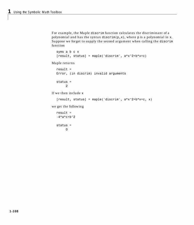
1 Using the Symbolic Math Toolbox
1-108
For example, the Maple discrim function calculates the discriminant of a polynomial and has the syntax discrim(p,x), where p is a polynomial in x. Suppose we forget to supply the second argument when calling the discrim function
syms a b c x[result, status] = maple('discrim', a*x^2+b*x+c)
Maple returns
result =Error, (in discrim) invalid arguments
status = 2
If we then include x
[result, status] = maple('discrim', a*x^2+b*x+c, x)
we get the following
result =-4*a*c+b^2
status = 0
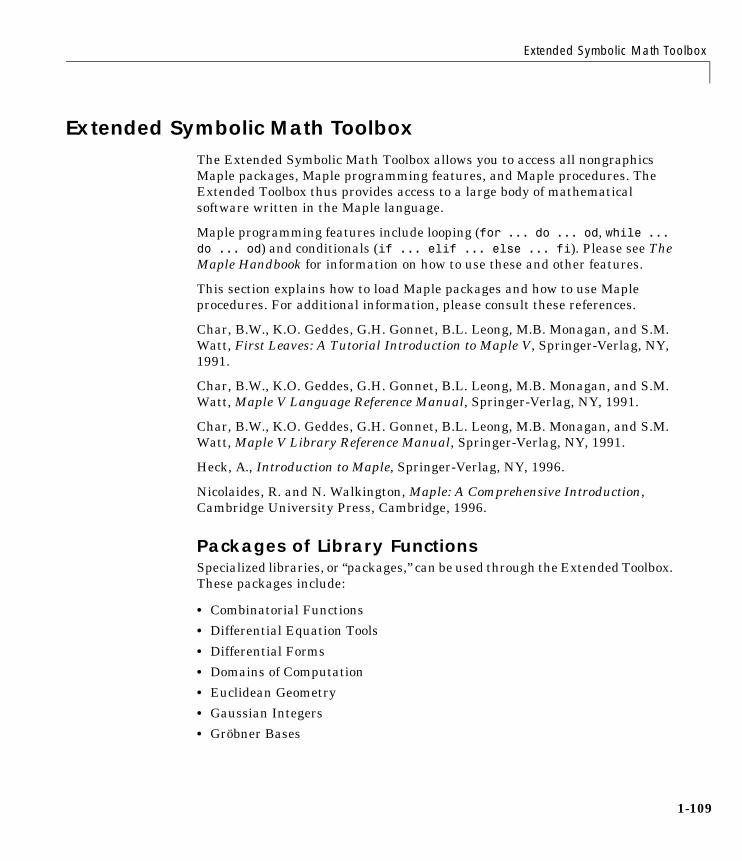
Extended Symbolic Math Toolbox
1-109
Extended Symbolic Math ToolboxThe Extended Symbolic Math Toolbox allows you to access all nongraphics Maple packages, Maple programming features, and Maple procedures. The Extended Toolbox thus provides access to a large body of mathematical software written in the Maple language.
Maple programming features include looping (for ... do ... od, while ... do ... od) and conditionals (if ... elif ... else ... fi). Please see The Maple Handbook for information on how to use these and other features.
This section explains how to load Maple packages and how to use Maple procedures. For additional information, please consult these references.
Char, B.W., K.O. Geddes, G.H. Gonnet, B.L. Leong, M.B. Monagan, and S.M. Watt, First Leaves: A Tutorial Introduction to Maple V, Springer-Verlag, NY, 1991.
Char, B.W., K.O. Geddes, G.H. Gonnet, B.L. Leong, M.B. Monagan, and S.M. Watt, Maple V Language Reference Manual, Springer-Verlag, NY, 1991.
Char, B.W., K.O. Geddes, G.H. Gonnet, B.L. Leong, M.B. Monagan, and S.M. Watt, Maple V Library Reference Manual, Springer-Verlag, NY, 1991.
Heck, A., Introduction to Maple, Springer-Verlag, NY, 1996.
Nicolaides, R. and N. Walkington, Maple: A Comprehensive Introduction, Cambridge University Press, Cambridge, 1996.
Packages of Library FunctionsSpecialized libraries, or “packages,” can be used through the Extended Toolbox. These packages include:
• Combinatorial Functions
• Differential Equation Tools
• Differential Forms
• Domains of Computation
• Euclidean Geometry
• Gaussian Integers
• Gröbner Bases

1 Using the Symbolic Math Toolbox
1-110
• Permutation and Finitely Presented Groups
• Lie Symmetries
• Boolean Logic
• Graph Networks
• Newman-Penrose Formalism
• Number Theory
• Numerical Approximation
• Orthogonal Polynomials
• p-adic Numbers
• Formal Power Series
• Projective Geometry
• Simplex Linear Optimization
• Statistics
• Total Orders on Names
• Galois Fields
• Linear Recurrence Relation Tools
• Financial Mathematics
• Rational Generating Functions
• Tensor Computations
You can use the Maple with command to load these packages. Say, for example, that you want to use the orthogonal polynomials package. First get the Maple name of this package, using the statement
mhelp index[packages]
which returns
Index of descriptions for packages of library functions
Description:- The following packages are available:
...orthopoly orthogonal polynomials ...
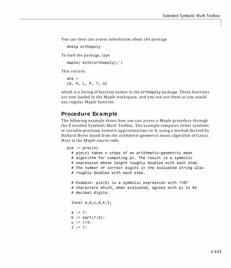
Extended Symbolic Math Toolbox
1-111
You can then can access information about the package
mhelp orthopoly
To load the package, type
maple('with(orthopoly);')
This returns
ans =[G, H, L, P, T, U]
which is a listing of function names in the orthopoly package. These functions are now loaded in the Maple workspace, and you can use them as you would any regular Maple function.
Procedure ExampleThe following example shows how you can access a Maple procedure through the Extended Symbolic Math Toolbox. The example computes either symbolic or variable-precision numeric approximations to , using a method derived by Richard Brent based from the arithmetic-geometric mean algorithm of Gauss. Here is the Maple source code.
pie := proc(n) # pie(n) takes n steps of an arithmetic–geometric mean # algorithm for computing pi. The result is a symbolic # expression whose length roughly doubles with each step. # The number of correct digits in the evaluated string also # roughly doubles with each step.
# Example: pie(5) is a symbolic expression with 1167 # characters which, when evaluated, agrees with pi to 84 # decimal digits.
local a,b,c,d,k,t;
a := 1: b := sqrt(1/2): c := 1/4: t := 1:
π

1 Using the Symbolic Math Toolbox
1-112
for k from 1 to n do d := (b-a)/2: b := sqrt(a*b): a := a+d: c := c-t*d^2: t := 2*t: od;
(a+b)^2/(4*c):
end;
Assume the source code for this Maple procedure is stored in the file pie.src. Using the Extended Symbolic Math Toolbox, the MATLAB statement
procread('pie.src')
reads the specified file, deletes comments and newline characters, and sends the resulting string to Maple. (The MATLAB ans variable then contains a string representation of the pie.src file.)
You can use the pie function, using the maple function. The statement
p = maple('pie',5)
returns a symbolic object p that begins and ends with
p = 1/4*(1/32+1/64*2^(1/2)+1/32*2^(3/4)+ ...
... *2^(1/2))*2^(3/4))^(1/2))^(1/2))^2)
It is interesting to change the computation from symbolic to numeric. The assignment to the variable b in the second executable line is key. If the assignment statement is simply
b := sqrt(1/2)
the entire computation is done symbolically. But if the assignment statement is modified to include decimal points
b := sqrt(1./2.)
the entire computation uses variable-precision arithmetic at the current setting of digits. If this change is made, then
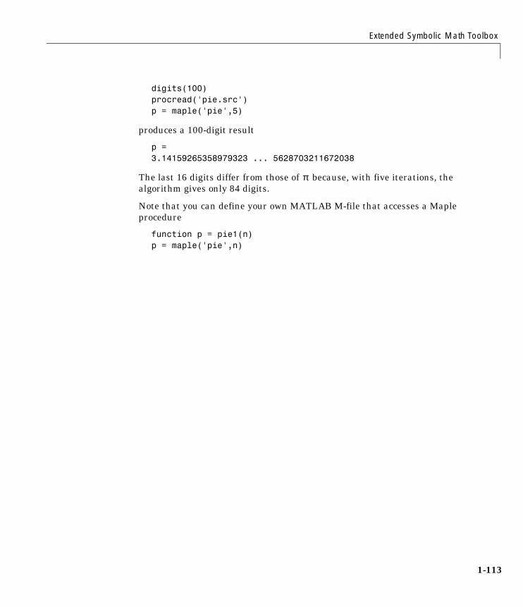
Extended Symbolic Math Toolbox
1-113
digits(100)procread('pie.src')p = maple('pie',5)
produces a 100-digit result
p =3.14159265358979323 ... 5628703211672038
The last 16 digits differ from those of because, with five iterations, the algorithm gives only 84 digits.
Note that you can define your own MATLAB M-file that accesses a Maple procedure
function p = pie1(n)p = maple('pie',n)
π

1 Using the Symbolic Math Toolbox
1-114
Precompiled Maple ProceduresWhen Maple loads a source (ASCII text) procedure into its workspace, it compiles (translates) the procedure into an internal format. You can subsequently use the maple function to save the procedures in the internal format. The advantage is you avoid recompiling the procedure the next time you load it, thereby speeding up the process.
For example, you can convert the pie.src procedure developed in the preceding example to a precompiled Maple procedure, using the commands
clear maplemexprocread('pie.src')maple('save(‘pi.m‘)');
The clear maplemex command resets the Maple workspace to its initial state. Since the Maple save command saves all variables in the current session, we want to remove extraneous variables. Note that you must use back quotes around the function name.
To read the precompiled procedure into a subsequent MATLAB session, type
maple('read','‘pie.m‘');
Again, as with the ASCII text form, you can access the function using maple
p = maple('pie',5)
Note that precompiled Maple procedures have .m extensions. Hence, you must take care to avoid confusing them with MATLAB M-files, which also have .m extensions.

2
Reference
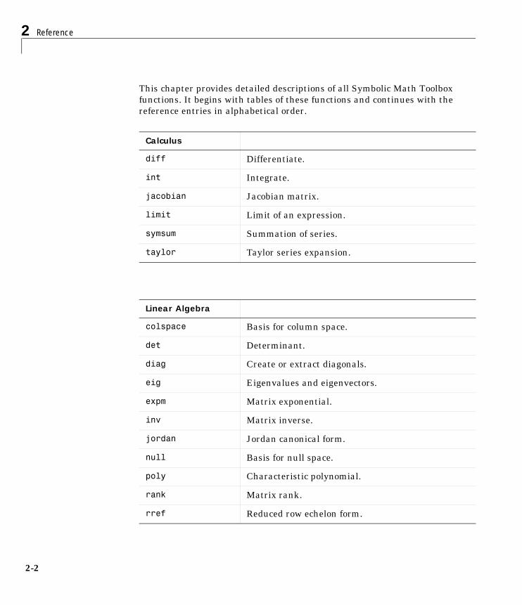
2 Reference
2-2
This chapter provides detailed descriptions of all Symbolic Math Toolbox functions. It begins with tables of these functions and continues with the reference entries in alphabetical order.
Calculus
diff Differentiate.
int Integrate.
jacobian Jacobian matrix.
limit Limit of an expression.
symsum Summation of series.
taylor Taylor series expansion.
Linear Algebra
colspace Basis for column space.
det Determinant.
diag Create or extract diagonals.
eig Eigenvalues and eigenvectors.
expm Matrix exponential.
inv Matrix inverse.
jordan Jordan canonical form.
null Basis for null space.
poly Characteristic polynomial.
rank Matrix rank.
rref Reduced row echelon form.

2-3
svd Singular value decomposition.
tril Lower triangle.
triu Upper triangle.
Simplification
collect Collect common terms.
expand Expand polynomials and elementary functions.
factor Factor.
horner Nested polynomial representation.
numden Numerator and denominator.
simple Search for shortest form.
simplify Simplification.
subexpr Rewrite in terms of subexpressions.
Solution of Equations
compose Functional composition.
dsolve Solution of differential equations.
finverse Functional inverse.
solve Solution of algebraic equations.
Linear Algebra
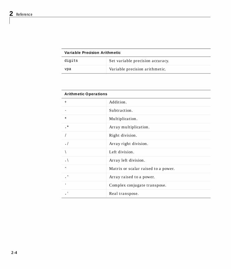
2 Reference
2-4
Variable Precision Arithmetic
digits Set variable precision accuracy.
vpa Variable precision arithmetic.
Arithmetic Operations
+ Addition.
- Subtraction.
* Multiplication.
.* Array multiplication.
/ Right division.
./ Array right division.
\ Left division.
.\ Array left division.
^ Matrix or scalar raised to a power.
.^ Array raised to a power.
' Complex conjugate transpose.
.' Real transpose.
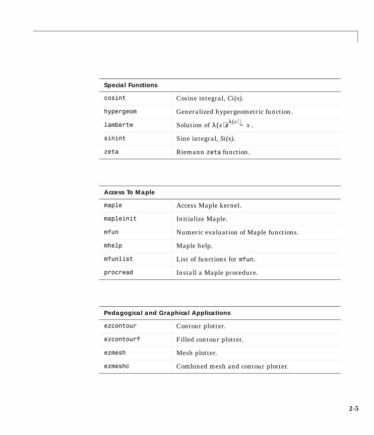
2-5
Special Functions
cosint Cosine integral, Ci(x).
hypergeom Generalized hypergeometric function.
lambertw Solution of .
sinint Sine integral, Si(x).
zeta Riemann zeta function.
Access To Maple
maple Access Maple kernel.
mapleinit Initialize Maple.
mfun Numeric evaluation of Maple functions.
mhelp Maple help.
mfunlist List of functions for mfun.
procread Install a Maple procedure.
Pedagogical and Graphical Applications
ezcontour Contour plotter.
ezcontourf Filled contour plotter.
ezmesh Mesh plotter.
ezmeshc Combined mesh and contour plotter.
λ x( )eλ x( ) x=
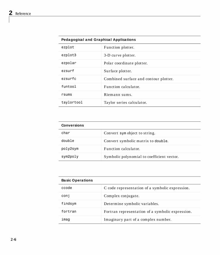
2 Reference
2-6
ezplot Function plotter.
ezplot3 3-D curve plotter.
ezpolar Polar coordinate plotter.
ezsurf Surface plotter.
ezsurfc Combined surface and contour plotter.
funtool Function calculator.
rsums Riemann sums.
taylortool Taylor series calculator.
Conversions
char Convert sym object to string.
double Convert symbolic matrix to double.
poly2sym Function calculator.
sym2poly Symbolic polynomial to coefficient vector.
Basic Operations
ccode C code representation of a symbolic expression.
conj Complex conjugate.
findsym Determine symbolic variables.
fortran Fortran representation of a symbolic expression.
imag Imaginary part of a complex number.
Pedagogical and Graphical Applications
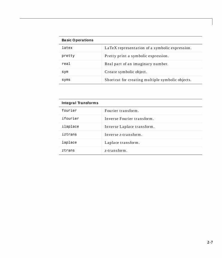
2-7
latex LaTeX representation of a symbolic expression.
pretty Pretty print a symbolic expression.
real Real part of an imaginary number.
sym Create symbolic object.
syms Shortcut for creating multiple symbolic objects.
Integral Transforms
fourier Fourier transform.
ifourier Inverse Fourier transform.
ilaplace Inverse Laplace transform.
iztrans Inverse z-transform.
laplace Laplace transform.
ztrans z-transform.
Basic Operations
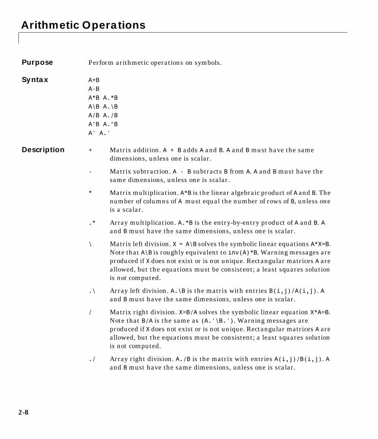
Arithmetic Operations
2-8
2Arithmetic OperationsPurpose Perform arithmetic operations on symbols.
Syntax A+BA-BA*B A.*BA\B A.\BA/B A./BA^B A.^BA' A.'
Description + Matrix addition. A + B adds A and B. A and B must have the same dimensions, unless one is scalar.
- Matrix subtraction. A - B subtracts B from A. A and B must have the same dimensions, unless one is scalar.
* Matrix multiplication. A*B is the linear algebraic product of A and B. The number of columns of A must equal the number of rows of B, unless one is a scalar.
.* Array multiplication. A.*B is the entry-by-entry product of A and B. A and B must have the same dimensions, unless one is scalar.
\ Matrix left division. X = A\B solves the symbolic linear equations A*X=B. Note that A\B is roughly equivalent to inv(A)*B. Warning messages are produced if X does not exist or is not unique. Rectangular matrices A are allowed, but the equations must be consistent; a least squares solution is not computed.
.\ Array left division. A.\B is the matrix with entries B(i,j)/A(i,j). A and B must have the same dimensions, unless one is scalar.
/ Matrix right division. X=B/A solves the symbolic linear equation X*A=B. Note that B/A is the same as (A.'\B.'). Warning messages are produced if X does not exist or is not unique. Rectangular matrices A are allowed, but the equations must be consistent; a least squares solution is not computed.
./ Array right division. A./B is the matrix with entries A(i,j)/B(i,j). A and B must have the same dimensions, unless one is scalar.
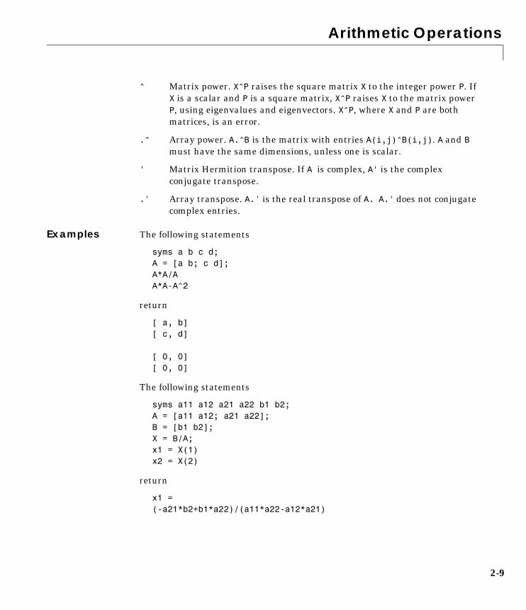
Arithmetic Operations
2-9
^ Matrix power. X^P raises the square matrix X to the integer power P. If X is a scalar and P is a square matrix, X^P raises X to the matrix power P, using eigenvalues and eigenvectors. X^P, where X and P are both matrices, is an error.
.^ Array power. A.^B is the matrix with entries A(i,j)^B(i,j). A and B must have the same dimensions, unless one is scalar.
' Matrix Hermition transpose. If A is complex, A' is the complex conjugate transpose.
.' Array transpose. A.' is the real transpose of A. A.' does not conjugate complex entries.
Examples The following statements
syms a b c d;A = [a b; c d];A*A/AA*A-A^2
return
[ a, b][ c, d]
[ 0, 0][ 0, 0]
The following statements
syms a11 a12 a21 a22 b1 b2;A = [a11 a12; a21 a22];B = [b1 b2];X = B/A;x1 = X(1)x2 = X(2)
return
x1 =(-a21*b2+b1*a22)/(a11*a22-a12*a21)
Arithmetic Operations
2-10
x2 =(a11*b2-a12*b1)/(a11*a22-a12*a21)
See Also null, solve

ccode
2-11
2ccodePurpose C code representation of a symbolic expression.
Syntax ccode(s)
Description ccode(s) returns a fragment of C that evaluates the symbolic expression s.
Examples The statements
syms xf = taylor(log(1+x));ccode(f)
return
t0 = x-x*x/2.0+x*x*x/3.0-x*x*x*x/4.0+x*x*x*x*x/5.0;
The statements
H = sym(hilb(3));ccode(H)
return
H[0][0] = 1.0; H[0][1] = 1.0/2.0; H[0][2] = 1.0/3.0;H[1][0] = 1.0/2.0; H[1][1] = 1.0/3.0; H[1][2] = 1.0/4.0;H[2][0] = 1.0/3.0; H[2][1] = 1.0/4.0; H[2][2] = 1.0/5.0;
See Also fortran, latex, pretty
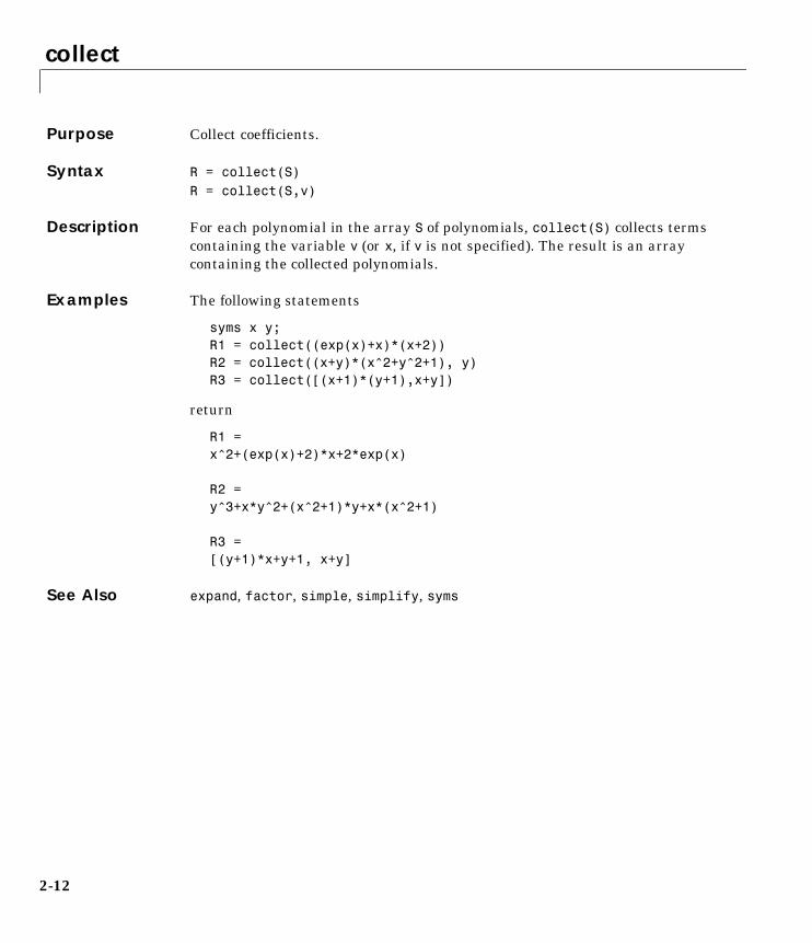
collect
2-12
2collectPurpose Collect coefficients.
Syntax R = collect(S)R = collect(S,v)
Description For each polynomial in the array S of polynomials, collect(S) collects terms containing the variable v (or x, if v is not specified). The result is an array containing the collected polynomials.
Examples The following statements
syms x y;R1 = collect((exp(x)+x)*(x+2))R2 = collect((x+y)*(x^2+y^2+1), y)R3 = collect([(x+1)*(y+1),x+y])
return
R1 = x^2+(exp(x)+2)*x+2*exp(x)
R2 = y^3+x*y^2+(x^2+1)*y+x*(x^2+1)
R3 = [(y+1)*x+y+1, x+y]
See Also expand, factor, simple, simplify, syms
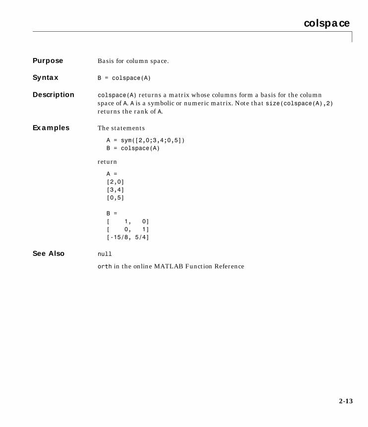
colspace
2-13
2colspacePurpose Basis for column space.
Syntax B = colspace(A)
Description colspace(A) returns a matrix whose columns form a basis for the column space of A. A is a symbolic or numeric matrix. Note that size(colspace(A),2) returns the rank of A.
Examples The statements
A = sym([2,0;3,4;0,5])B = colspace(A)
return
A =[2,0][3,4][0,5]
B =[ 1, 0][ 0, 1][-15/8, 5/4]
See Also null
orth in the online MATLAB Function Reference
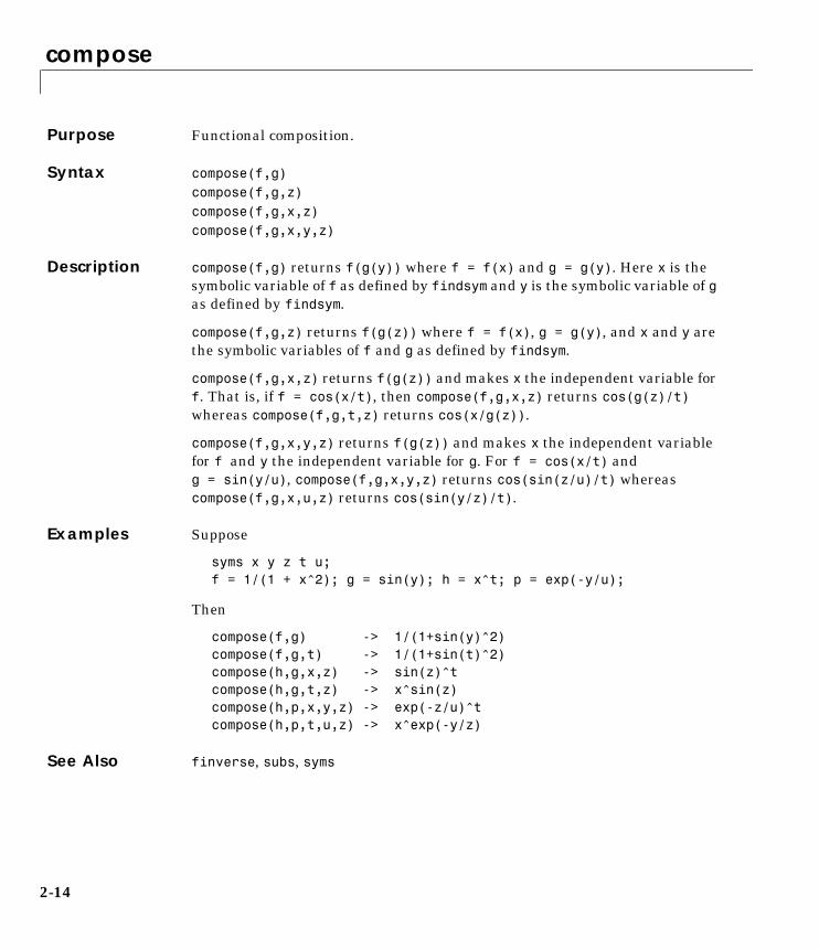
compose
2-14
2composePurpose Functional composition.
Syntax compose(f,g)compose(f,g,z)compose(f,g,x,z)compose(f,g,x,y,z)
Description compose(f,g) returns f(g(y)) where f = f(x) and g = g(y). Here x is the symbolic variable of f as defined by findsym and y is the symbolic variable of g as defined by findsym.
compose(f,g,z) returns f(g(z)) where f = f(x), g = g(y), and x and y are the symbolic variables of f and g as defined by findsym.
compose(f,g,x,z) returns f(g(z)) and makes x the independent variable for f. That is, if f = cos(x/t), then compose(f,g,x,z) returns cos(g(z)/t) whereas compose(f,g,t,z) returns cos(x/g(z)).
compose(f,g,x,y,z) returns f(g(z)) and makes x the independent variable for f and y the independent variable for g. For f = cos(x/t) andg = sin(y/u), compose(f,g,x,y,z) returns cos(sin(z/u)/t) whereas compose(f,g,x,u,z) returns cos(sin(y/z)/t).
Examples Suppose
syms x y z t u;f = 1/(1 + x^2); g = sin(y); h = x^t; p = exp(-y/u);
Then
compose(f,g) -> 1/(1+sin(y)^2) compose(f,g,t) -> 1/(1+sin(t)^2)compose(h,g,x,z) -> sin(z)^tcompose(h,g,t,z) -> x^sin(z)compose(h,p,x,y,z) -> exp(-z/u)^t compose(h,p,t,u,z) -> x^exp(-y/z)
See Also finverse, subs, syms

conj
2-15
2conjPurpose Symbolic conjugate.
Syntax conj(X)
Description conj(X) is the complex conjugate of X.
For a complex X, conj(X) = real(X) - i*imag(X).
See Also real, imag

cosint
2-16
2cosintPurpose Cosine integral function.
Syntax Y = cosint(X)
Description cosint(X) evaluates the cosine integral function at the elements of X, a numeric matrix, or a symbolic matrix. The cosine integral function is defined by
where is Euler’s constant 0.577215664...
Examples cosint(7.2) returns 0.0960.
cosint([0:0.1:1]) returns
Columns 1 through 7
Inf -1.7279 -1.0422 -0.6492 -0.3788 -0.1778 -0.0223 Columns 8 through 11 0.1005 0.1983 0.2761 0.3374
The statements
syms x;f = cosint(x);diff(f)
return
cos(x)/x
See Also sinint
Ci x( ) γ x( )ln tcos 1–t
-------------------- td
0
x
∫+ +=
γ
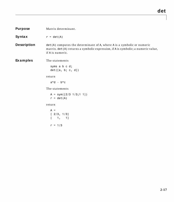
det
2-17
2detPurpose Matrix determinant.
Syntax r = det(A)
Description det(A) computes the determinant of A, where A is a symbolic or numeric matrix. det(A) returns a symbolic expression, if A is symbolic; a numeric value, if A is numeric.
Examples The statements
syms a b c d;det([a, b; c, d])
return
a*d - b*c
The statements
A = sym([2/3 1/3;1 1])r = det(A)
return
A =[ 2/3, 1/3][ 1, 1]
r = 1/3
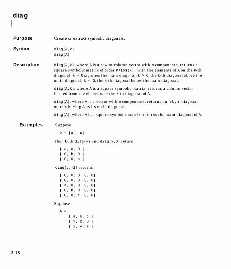
diag
2-18
2diagPurpose Create or extract symbolic diagonals.
Syntax diag(A,k)diag(A)
Description diag(A,k), where A is a row or column vector with n components, returns a square symbolic matrix of order n+abs(k), with the elements of A on the k-th diagonal. k = 0 signifies the main diagonal; k > 0, the k-th diagonal above the main diagonal; k < 0, the k-th diagonal below the main diagonal.
diag(A,k), where A is a square symbolic matrix, returns a column vector formed from the elements of the k-th diagonal of A.
diag(A), where A is a vector with n components, returns an n-by-n diagonal matrix having A as its main diagonal.
diag(A), where A is a square symbolic matrix, returns the main diagonal of A.
Examples Suppose
v = [a b c]
Then both diag(v) and diag(v,0) return
[ a, 0, 0 ][ 0, b, 0 ][ 0, 0, c ]
diag(v,-2) returns
[ 0, 0, 0, 0, 0][ 0, 0, 0, 0, 0][ a, 0, 0, 0, 0][ 0, b, 0, 0, 0][ 0, 0, c, 0, 0]
Suppose
A =[ a, b, c ][ 1, 2, 3 ][ x, y, z ]
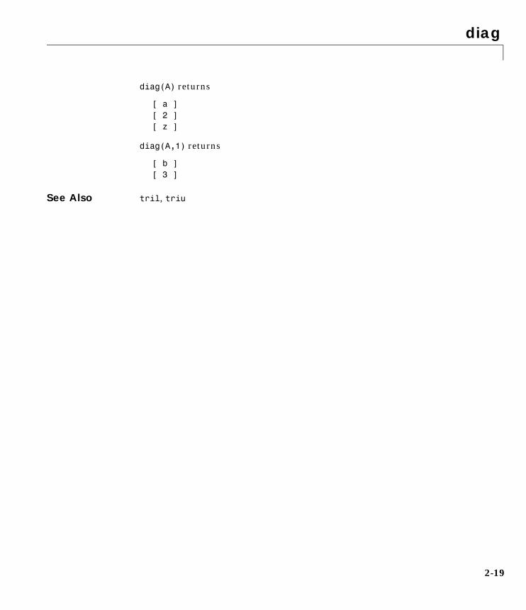
diag
2-19
diag(A) returns
[ a ][ 2 ][ z ]
diag(A,1) returns
[ b ][ 3 ]
See Also tril, triu
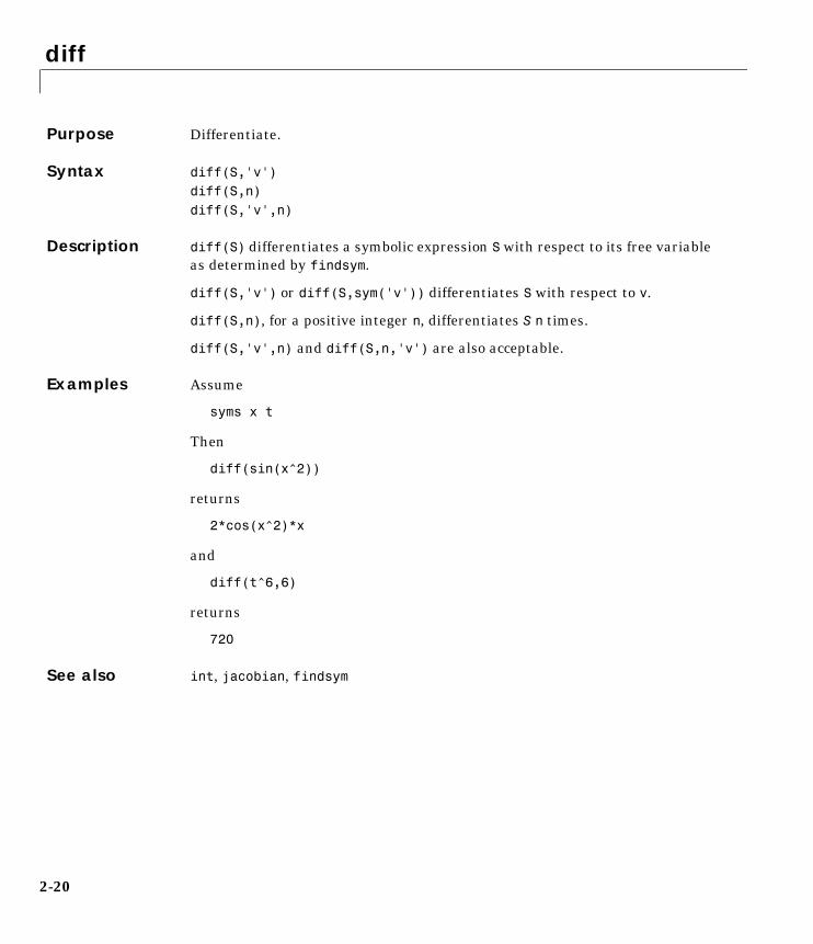
diff
2-20
2diffPurpose Differentiate.
Syntax diff(S,'v')diff(S,n)diff(S,'v',n)
Description diff(S) differentiates a symbolic expression S with respect to its free variable as determined by findsym.
diff(S,'v') or diff(S,sym('v')) differentiates S with respect to v.
diff(S,n), for a positive integer n, differentiates S n times.
diff(S,'v',n) and diff(S,n,'v') are also acceptable.
Examples Assume
syms x t
Then
diff(sin(x^2))
returns
2*cos(x^2)*x
and
diff(t^6,6)
returns
720
See also int, jacobian, findsym
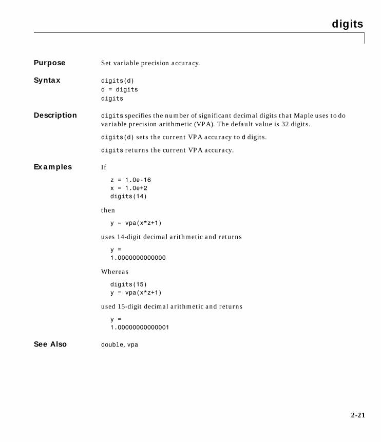
digits
2-21
2digitsPurpose Set variable precision accuracy.
Syntax digits(d)d = digitsdigits
Description digits specifies the number of significant decimal digits that Maple uses to do variable precision arithmetic (VPA). The default value is 32 digits.
digits(d) sets the current VPA accuracy to d digits.
digits returns the current VPA accuracy.
Examples If
z = 1.0e-16x = 1.0e+2digits(14)
then
y = vpa(x*z+1)
uses 14-digit decimal arithmetic and returns
y =1.0000000000000
Whereas
digits(15)y = vpa(x*z+1)
used 15-digit decimal arithmetic and returns
y =1.00000000000001
See Also double, vpa
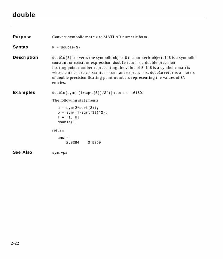
double
2-22
2doublePurpose Convert symbolic matrix to MATLAB numeric form.
Syntax R = double(S)
Description double(S) converts the symbolic object S to a numeric object. If S is a symbolic constant or constant expression, double returns a double-precision floating-point number representing the value of S. If S is a symbolic matrix whose entries are constants or constant expressions, double returns a matrix of double precision floating-point numbers representing the values of S’s entries.
Examples double(sym('(1+sqrt(5))/2')) returns 1.6180.
The following statements
a = sym(2*sqrt(2));b = sym((1-sqrt(3))^2);T = [a, b]double(T)
return
ans =2.8284 0.5359
See Also sym, vpa
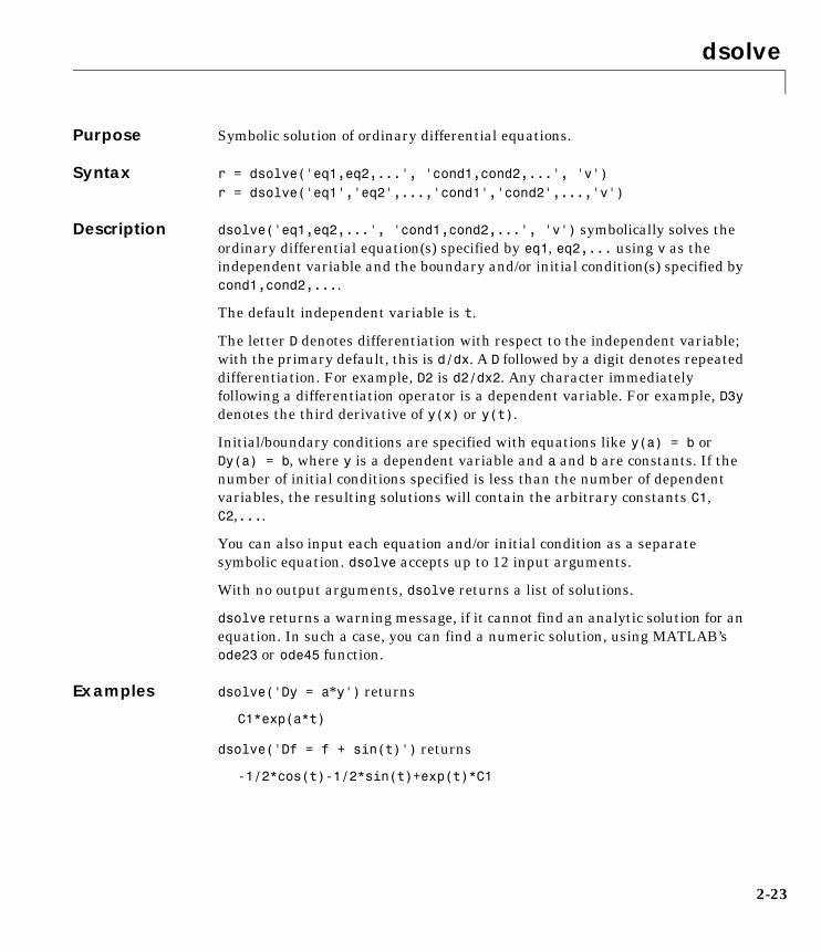
dsolve
2-23
2dsolvePurpose Symbolic solution of ordinary differential equations.
Syntax r = dsolve('eq1,eq2,...', 'cond1,cond2,...', 'v')r = dsolve('eq1','eq2',...,'cond1','cond2',...,'v')
Description dsolve('eq1,eq2,...', 'cond1,cond2,...', 'v') symbolically solves the ordinary differential equation(s) specified by eq1, eq2,... using v as the independent variable and the boundary and/or initial condition(s) specified by cond1,cond2,....
The default independent variable is t.
The letter D denotes differentiation with respect to the independent variable; with the primary default, this is d/dx. A D followed by a digit denotes repeated differentiation. For example, D2 is d2/dx2. Any character immediately following a differentiation operator is a dependent variable. For example, D3y denotes the third derivative of y(x) or y(t).
Initial/boundary conditions are specified with equations like y(a) = b or Dy(a) = b, where y is a dependent variable and a and b are constants. If the number of initial conditions specified is less than the number of dependent variables, the resulting solutions will contain the arbitrary constants C1, C2,....
You can also input each equation and/or initial condition as a separate symbolic equation. dsolve accepts up to 12 input arguments.
With no output arguments, dsolve returns a list of solutions.
dsolve returns a warning message, if it cannot find an analytic solution for an equation. In such a case, you can find a numeric solution, using MATLAB’s ode23 or ode45 function.
Examples dsolve('Dy = a*y') returns
C1*exp(a*t)
dsolve('Df = f + sin(t)') returns
-1/2*cos(t)-1/2*sin(t)+exp(t)*C1
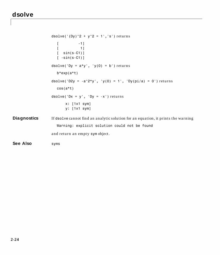
dsolve
2-24
dsolve('(Dy)^2 + y^2 = 1','s') returns
[ -1][ 1][ sin(s-C1)][ -sin(s-C1)]
dsolve('Dy = a*y', 'y(0) = b') returns
b*exp(a*t)
dsolve('D2y = -a^2*y', 'y(0) = 1', 'Dy(pi/a) = 0') returns
cos(a*t)
dsolve('Dx = y', 'Dy = -x') returns
x: [1x1 sym] y: [1x1 sym]
Diagnostics If dsolve cannot find an analytic solution for an equation, it prints the warning
Warning: explicit solution could not be found
and return an empty sym object.
See Also syms
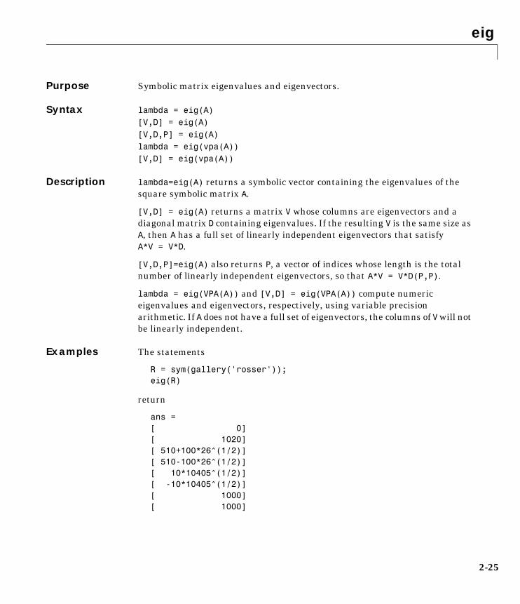
eig
2-25
2eigPurpose Symbolic matrix eigenvalues and eigenvectors.
Syntax lambda = eig(A)[V,D] = eig(A)[V,D,P] = eig(A)lambda = eig(vpa(A))[V,D] = eig(vpa(A))
Description lambda=eig(A) returns a symbolic vector containing the eigenvalues of the square symbolic matrix A.
[V,D] = eig(A) returns a matrix V whose columns are eigenvectors and a diagonal matrix D containing eigenvalues. If the resulting V is the same size as A, then A has a full set of linearly independent eigenvectors that satisfy A*V = V*D.
[V,D,P]=eig(A) also returns P, a vector of indices whose length is the total number of linearly independent eigenvectors, so that A*V = V*D(P,P).
lambda = eig(VPA(A)) and [V,D] = eig(VPA(A)) compute numeric eigenvalues and eigenvectors, respectively, using variable precision arithmetic. If A does not have a full set of eigenvectors, the columns of V will not be linearly independent.
Examples The statements
R = sym(gallery('rosser'));eig(R)
return
ans =[ 0][ 1020][ 510+100*26^(1/2)][ 510-100*26^(1/2)][ 10*10405^(1/2)][ -10*10405^(1/2)][ 1000][ 1000]

eig
2-26
eig(vpa(R)) returns
ans =
[ -1020.0490184299968238463137913055][ .56512999999999999999999999999800e-28][ .98048640721516997177589097485157e-1][ 1000.0000000000000000000000000002][ 1000.0000000000000000000000000003][ 1019.9019513592784830028224109024][ 1020.0000000000000000000000000003][ 1020.0490184299968238463137913055]
The statements
A = sym(gallery(5));[v,lambda] = eig(A)
return
v =[ 0][ 21/256][ -71/128][ 973/256][ 1]
lambda = [ 0, 0, 0, 0, 0][ 0, 0, 0, 0, 0][ 0, 0, 0, 0, 0][ 0, 0, 0, 0, 0][ 0, 0, 0, 0, 0]
See Also jordan, poly, svd, vpa

expm
2-27
2expmPurpose Symbolic matrix exponential.
Syntax expm(A)
Description expm(A) is the matrix exponential of the symbolic matrix A.
Examples The statements
syms t;A = [0 1; -1 0];expm(t*A)
return
[ cos(t), sin(t)][ -sin(t), cos(t)]

expand
2-28
2expandPurpose Symbolic expansion.
Syntax R = expand(S)
Description expand(S) writes each element of a symbolic expression S as a product of its factors. expand is most often used only with polynomials, but also expands trigonometric, exponential, and logarithmic functions.
Examples expand((x-2)*(x-4)) returns
x^2-6*x+8
expand(cos(x+y)) returns
cos(x)*cos(y)-sin(x)*sin(y)
expand(exp((a+b)^2)) returns
exp(a^2)*exp(a*b)^2*exp(b^2)
expand([sin(2*t), cos(2*t)]) returns
[2*sin(t)*cos(t), 2*cos(t)^2-1]
See Also collect, factor, horner, simple, simplify, syms

ezcontour
2-29
2ezcontourPurpose Contour plotter.
Syntax ezcontour(f)ezcontour(f,domain)ezcontour(...,n)
Description ezcontour(f) plots the contour lines of f(x,y), where f is a symbolic expression that represents a mathematical function of two variables, such as x and y.
The function f is plotted over the default domain , . MATLAB chooses the computational grid according to the amount of variation that occurs; if the function f is not defined (singular) for points on the grid, then these points are not plotted.
ezcontour(f,domain) plots f(x,y) over the specified domain. domain can be either a 4-by-1 vector [xmin, xmax, ymin, ymax] or a 2-by-1 vector [min, max] (where, min < x < max, min < y < max).
If f is a function of the variables u and v (rather than x and y), then the domain endpoints umin, umax, vmin, and vmax are sorted alphabetically. Thus, ezcontour(u^2 - v^3,[0,1],[3,6]) plots the contour lines for u2 - v3 over0 < u < 1, 3 < v < 6.
ezcontour(...,n) plots f over the default domain using an n-by-n grid. The default value for n is 60.
ezcontour automatically adds a title and axis labels.
Examples The following mathematical expression defines a function of two variables, x and y.
ezcontour requires a sym argument that expresses this function using MATLAB syntax to represent exponents, natural logs, etc. This function is represented by the symbolic expression
syms x yf = 3*(1-x)^2*exp(-(x^2)-(y+1)^2) ... - 10*(x/5 - x^3 - y^5)*exp(-x^2-y^2) ... - 1/3*exp(-(x+1)^2 - y^2);
2π– x 2π< < 2π– y 2π< <
f x y,( ) 3 1 x–( )2e x2– y 1+( )2– 10 x5--- x3– y5–
e x2– y2––13---e x 1+( )2– y2––=
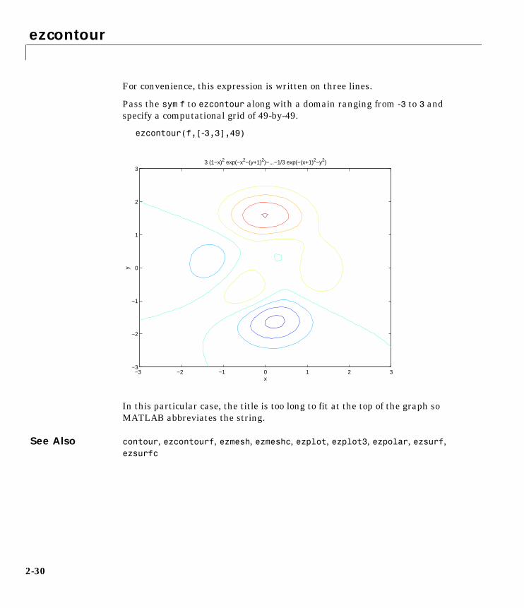
ezcontour
2-30
For convenience, this expression is written on three lines.
Pass the sym f to ezcontour along with a domain ranging from -3 to 3 and specify a computational grid of 49-by-49.
ezcontour(f,[-3,3],49)
In this particular case, the title is too long to fit at the top of the graph so MATLAB abbreviates the string.
See Also contour, ezcontourf, ezmesh, ezmeshc, ezplot, ezplot3, ezpolar, ezsurf, ezsurfc
−3 −2 −1 0 1 2 3−3
−2
−1
0
1
2
3
x
y
3 (1−x)2 exp(−x2−(y+1)2)−...−1/3 exp(−(x+1)2−y2)
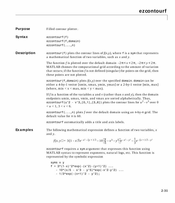
ezcontourf
2-31
2ezcontourfPurpose Filled contour plotter.
Syntax ezcontourf(f)ezcontourf(f,domain)ezcontourf(...,n)
Description ezcontour(f) plots the contour lines of f(x,y), where f is a sym that represents a mathematical function of two variables, such as x and y.
The function f is plotted over the default domain , . MATLAB chooses the computational grid according to the amount of variation that occurs; if the function f is not defined (singular) for points on the grid, then these points are not plotted.
ezcontour(f,domain) plots f(x,y) over the specified domain. domain can be either a 4-by-1 vector [xmin, xmax, ymin, ymax] or a 2-by-1 vector [min, max] (where, min < x < max, min < y < max).
If f is a function of the variables u and v (rather than x and y), then the domain endpoints umin, umax, vmin, and vmax are sorted alphabetically. Thus, ezcontourf(u^2 - v^3,[0,1],[3,6]) plots the contour lines for u2 - v3 over 0 < u < 1, 3 < v < 6.
ezcontourf(...,n) plots f over the default domain using an n-by-n grid. The default value for n is 60.
ezcontourf automatically adds a title and axis labels.
Examples The following mathematical expression defines a function of two variables, x and y.
ezcontourf requires a sym argument that expresses this function using MATLAB syntax to represent exponents, natural logs, etc. This function is represented by the symbolic expression
syms x yf = 3*(1-x)^2*exp(-(x^2)-(y+1)^2) ... - 10*(x/5 - x^3 - y^5)*exp(-x^2-y^2) ... - 1/3*exp(-(x+1)^2 - y^2);
2π– x 2π< < 2π– y 2π< <
f x y,( ) 3 1 x–( )2e x2– y 1+( )2– 10 x5--- x3– y5–
e x2– y2––13---e x 1+( )2– y2––=

ezcontourf
2-32
For convenience, this expression is written on three lines.
Pass the sym f to ezcontourf along with a domain ranging from -3 to 3 and specify a grid of 49-by-49.
ezcontourf(f,[-3,3],49)
In this particular case, the title is too long to fit at the top of the graph so MATLAB abbreviates the string.
See Also contourf, ezcontour, ezmesh, ezmeshc, ezplot, ezplot3, ezpolar, ezsurf, ezsurfc
−3 −2 −1 0 1 2 3−3
−2
−1
0
1
2
3
x
y
3 (1−x)2 exp(−x2−(y+1)2)−...−1/3 exp(−(x+1)2−y2)
ezmesh
2-33
2ezmeshPurpose 3-D mesh plotter.
Syntax ezmesh(f)ezmesh(f,domain)ezmesh(x,y,z)ezmesh(x,y,z,[smin,smax,tmin,tmax]) or ezmesh(x,y,z,[min,max])ezmesh(...,n)ezmesh(...,'circ')
Description ezmesh(f) creates a graph of f(x,y), where f is a symbolic expression that represents a mathematical function of two variables, such as x and y.
The function f is plotted over the default domain , . MATLAB chooses the computational grid according to the amount of variation that occurs; if the function f is not defined (singular) for points on the grid, then these points are not plotted.
ezmesh(f,domain) plots f over the specified domain. domain can be either a 4-by-1 vector [xmin, xmax, ymin, ymax] or a 2-by-1 vector [min, max] (where, min < x < max, min < y < max).
If f is a function of the variables u and v (rather than x and y), then the domain endpoints umin, umax, vmin, and vmax are sorted alphabetically. Thus, ezmesh(u^2 - v^3,[0,1],[3,6]) plots u2 - v3 over 0 < u < 1, 3 < v < 6.
ezmesh(x,y,z) plots the parametric surface x = x(s,t), y = y(s,t), and z = z(s,t) over the square , .
ezmesh(x,y,z,[smin,smax,tmin,tmax]) or ezmesh(x,y,z,[min,max]) plots the parametric surface using the specified domain.
ezmesh(...,n) plots f over the default domain using an n-by-n grid. The default value for n is 60.
ezmesh(...,'circ') plots f over a disk centered on the domain
Remarks rotate3d is always on. To rotate the graph, click and drag with the mouse.
Examples This example visualizes the function,
2π– x 2π< < 2π– y 2π< <
2π– s 2π< < 2π– t 2π< <
f x y,( ) xe x– 2 y2–=
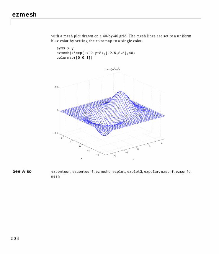
ezmesh
2-34
with a mesh plot drawn on a 40-by-40 grid. The mesh lines are set to a uniform blue color by setting the colormap to a single color.
syms x yezmesh(x*exp(-x^2-y^2),[-2.5,2.5],40)colormap([0 0 1])
See Also ezcontour, ezcontourf, ezmeshc, ezplot, ezplot3, ezpolar, ezsurf, ezsurfc, mesh
−2−1
01
2
−2
−1
0
1
2
−0.5
0
0.5
x
x exp(−x2−y2)
y
ezmeshc
2-35
2ezmeshcPurpose Combined mesh/contour plotter.
Syntax ezmeshc(f)ezmeshc(f,domain)ezmeshc(x,y,z)ezmeshc(x,y,z,[smin,smax,tmin,tmax]) or ezmeshc(x,y,z,[min,max])ezmeshc(...,n)ezmeshc(...,'circ')
Description ezmeshc(f) creates a graph of f(x,y), where f is a symbolic expression that represents a mathematical function of two variables, such as x and y.
The function f is plotted over the default domain , . MATLAB chooses the computational grid according to the amount of variation that occurs; if the function f is not defined (singular) for points on the grid, then these points are not plotted.
ezmeshc(f,domain) plots f over the specified domain. domain can be either a 4-by-1 vector [xmin, xmax, ymin, ymax] or a 2-by-1 vector [min, max] (where, min < x < max, min < y < max).
If f is a function of the variables u and v (rather than x and y), then the domain endpoints umin, umax, vmin, and vmax are sorted alphabetically. Thus, ezmeshc(u^2 - v^3,[0,1],[3,6]) plots u2 - v3 over 0 < u < 1, 3 < v < 6.
ezmeshc(x,y,z) plots the parametric surface x = x(s,t), y = y(s,t), and z = z(s,t) over the square , .
ezmeshc(x,y,z,[smin,smax,tmin,tmax]) or ezmeshc(x,y,z,[min,max]) plots the parametric surface using the specified domain.
ezmeshc(...,n) plots f over the default domain using an n-by-n grid. The default value for n is 60.
ezmeshc(...,'circ') plots f over a disk centered on the domain
Remarks rotate3d is always on. To rotate the graph, click and drag with the mouse.
Examples Create a mesh/contour graph of the expression,
2π– x 2π< < 2π– y 2π< <
2π– s 2π< < 2π– t 2π< <
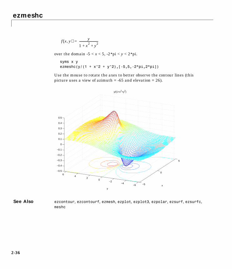
ezmeshc
2-36
over the domain -5 < x < 5, -2*pi < y < 2*pi.
syms x yezmeshc(y/(1 + x^2 + y^2),[-5,5,-2*pi,2*pi])
Use the mouse to rotate the axes to better observe the contour lines (this picture uses a view of azimuth = -65 and elevation = 26).
See Also ezcontour, ezcontourf, ezmesh, ezplot, ezplot3, ezpolar, ezsurf, ezsurfc, meshc
f x y,( ) y
1 x2 y2+ +
---------------------------=
−5
0
5
−6−4
−20
24
6−0.5
−0.4
−0.3
−0.2
−0.1
0
0.1
0.2
0.3
0.4
0.5
x
y/(1+x2+y2)
y
ezplot
2-37
2ezplotPurpose Function plotter.
Syntax ezplot(f)ezplot(f,[min,max])ezplot(f,[xmin,xmax,ymin,ymax])ezplot(x,y)ezplot(x,y,[tmin,tmax])ezplot(...,figure)
Description ezplot(f) plots the expression f = f(x) over the default domain .
ezplot(f,[xmin xmax]) plots f = f(x) over the specified domain. It opens and displays the result in a window labeled Figure No. 1. If any plot windows are already open, ezplot displays the result in the highest numbered window.
ezplot(f,[xmin xmax],fign) opens (if necessary) and displays the plot in the window labeled fign.
For implicitly defined functions, f = f(x,y).
ezplot(f) plots f(x,y) = 0 over the default domain , .
ezplot(f,[xmin,xmax,ymin,ymax]) plots f(x,y) = 0 over xmin < x < xmax and ymin < y < ymax.
ezplot(f,[min,max])plots f(x,y) = 0 over min < x < max and min < y < max.
If f is a function of the variables u and v (rather than x and y), then the domain endpoints umin, umax, vmin, and vmax are sorted alphabetically. Thus, ezplot(u^2 - v^2 - 1,[-3,2,-2,3]) plots u2 - v2 - 1 = 0 over -3 < u < 2, -2 < v < 3.
ezplot(x,y) plots the parametrically defined planar curve x = x(t) and y = y(t) over the default domain .
ezplot(x,y,[tmin,tmax]) plots x = x(t) and y = y(t) over tmin < t < tmax.
ezplot(...,figure) plots the given function over the specified domain in the figure window identified by the handle figure.
Algorithm If you do not specify a plot range, ezplot samples the function between -2*pi and 2*pi and selects a subinterval where the variation is significant as the plot
2π– x 2π< <
2π– x 2π< < 2π– y 2π< <
0 t 2π< <
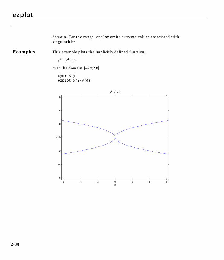
ezplot
2-38
domain. For the range, ezplot omits extreme values associated with singularities.
Examples This example plots the implicitly defined function,
x2 - y4 = 0
over the domain
syms x yezplot(x^2-y^4)
2π– 2π[ , ]
−6 −4 −2 0 2 4 6
−6
−4
−2
0
2
4
6
x
y
x2−y4 = 0
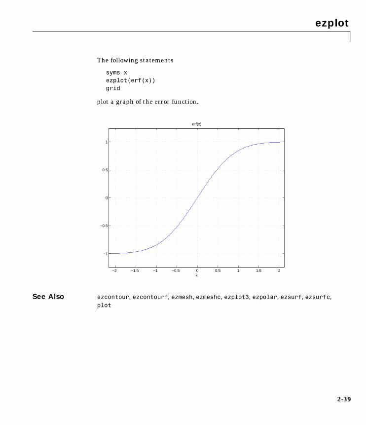
ezplot
2-39
The following statements
syms xezplot(erf(x))grid
plot a graph of the error function.
See Also ezcontour, ezcontourf, ezmesh, ezmeshc, ezplot3, ezpolar, ezsurf, ezsurfc, plot
−2 −1.5 −1 −0.5 0 0.5 1 1.5 2
−1
−0.5
0
0.5
1
x
erf(x)
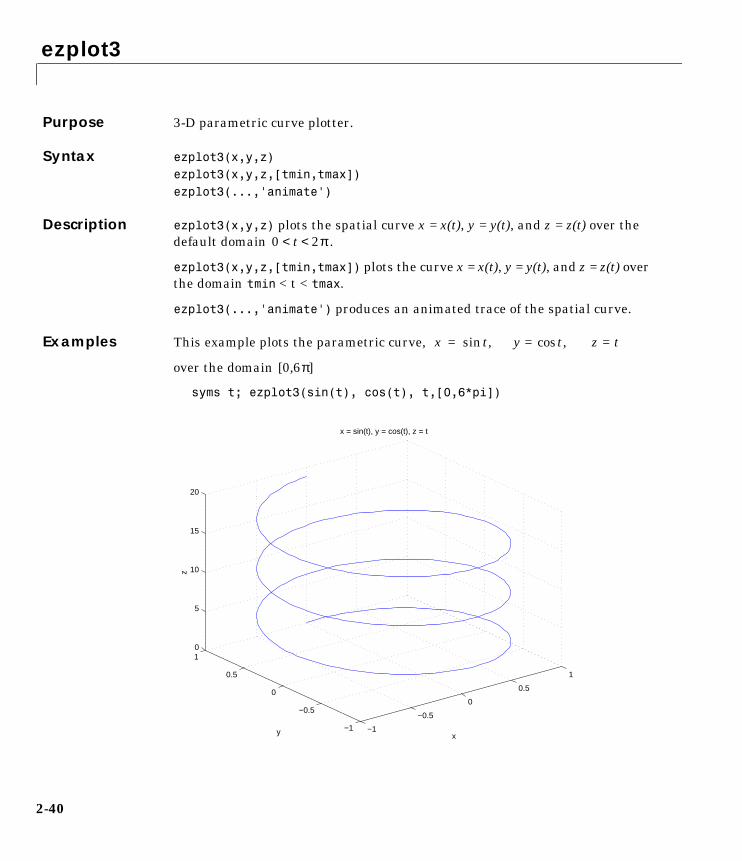
ezplot3
2-40
2ezplot3Purpose 3-D parametric curve plotter.
Syntax ezplot3(x,y,z)ezplot3(x,y,z,[tmin,tmax])ezplot3(...,'animate')
Description ezplot3(x,y,z) plots the spatial curve x = x(t), y = y(t), and z = z(t) over the default domain .
ezplot3(x,y,z,[tmin,tmax]) plots the curve x = x(t), y = y(t), and z = z(t) over the domain tmin < t < tmax.
ezplot3(...,'animate') produces an animated trace of the spatial curve.
Examples This example plots the parametric curve,
over the domain
syms t; ezplot3(sin(t), cos(t), t,[0,6*pi])
0 t 2π< <
x t y t z t=,cos=,sin=
0 6π[ , ]
−1
−0.5
0
0.5
1
−1
−0.5
0
0.5
10
5
10
15
20
x
x = sin(t), y = cos(t), z = t
y
z
ezplot3
2-41
See Also ezcontour, ezcontourf, ezmesh, ezmeshc, ezplot, ezpolar, ezsurf, ezsurfc, plot3
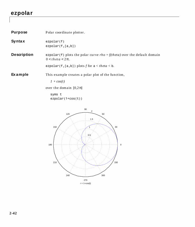
ezpolar
2-42
2ezpolarPurpose Polar coordinate plotter.
Syntax ezpolar(f)ezpolar(f,[a,b])
Description ezpolar(f) plots the polar curve rho = f(theta) over the default domain .
ezpolar(f,[a,b]) plots f for a < theta < b.
Example This example creates a polar plot of the function,
1 + cos(t)
over the domain
syms tezpolar(1+cos(t))
0 theta 2π< <
0 2π[ , ]
0.5
1
1.5
2
30
210
60
240
90
270
120
300
150
330
180 0
r = 1+cos(t)
ezsurf
2-43
2ezsurfPurpose 3-D colored surface plotter.
Syntax ezsurf(f)ezsurf(f,domain)ezsurf(x,y,z)ezsurf(x,y,z,[smin,smax,tmin,tmax]) or ezsurf(x,y,z,[min,max])ezsurf(...,n)ezsurf(...,'circ')
Purpose ezsurf(f) creates a graph of f(x,y), where f is a symbolic expression that represents a mathematical function of two variables, such as x and y.
The function f is plotted over the default domain , . MATLAB chooses the computational grid according to the amount of variation that occurs; if the function f is not defined (singular) for points on the grid, then these points are not plotted.
ezsurf(f,domain) plots f over the specified domain. domain can be either a 4-by-1 vector [xmin, xmax, ymin, ymax] or a 2-by-1 vector [min, max] (where, min < x < max, min < y < max).
If f is a function of the variables u and v (rather than x and y), then the domain endpoints umin, umax, vmin, and vmax are sorted alphabetically. Thus, ezsurf(u^2 - v^3,[0,1],[3,6]) plots u2 - v3 over 0 < u < 1, 3 < v < 6.
ezsurf(x,y,z) plots the parametric surface x = x(s,t), y = y(s,t), and z = z(s,t) over the square , .
ezsurf(x,y,z,[smin,smax,tmin,tmax]) or ezsurf(x,y,z,[min,max]) plots the parametric surface using the specified domain.
ezsurf(...,n) plots f over the default domain using an n-by-n grid. The default value for n is 60.
ezsurf(...,'circ') plots f over a disk centered on the domain
Remarks rotate3d is always on. To rotate the graph, click and drag with the mouse.
Examples ezsurf does not graph points where the mathematical function is not defined (these data points are set to NaNs, which MATLAB does not plot). This example
2π– x 2π< < 2π– y 2π< <
2π– s 2π< < 2π– t 2π< <
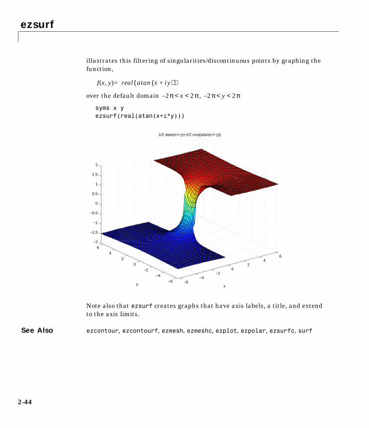
ezsurf
2-44
illustrates this filtering of singularities/discontinuous points by graphing the function,
over the default domain ,
syms x yezsurf(real(atan(x+i*y)))
Note also that ezsurf creates graphs that have axis labels, a title, and extend to the axis limits.
See Also ezcontour, ezcontourf, ezmesh, ezmeshc, ezplot, ezpolar, ezsurfc, surf
f x y,( ) x iy+( )atan( )real=
2π– x 2π< < 2π– y 2π< <
−6−4
−20
24
6
−6−4
−20
24
6−2
−1.5
−1
−0.5
0
0.5
1
1.5
2
x
1/2 atan(x+i y)+1/2 conj(atan(x+i y))
y
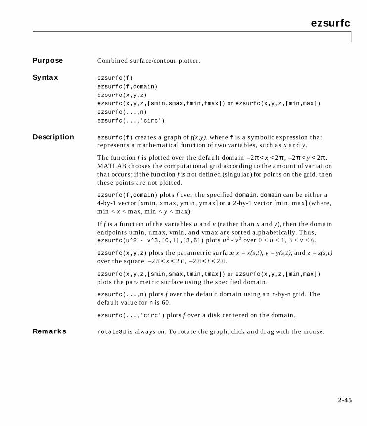
ezsurfc
2-45
2ezsurfcPurpose Combined surface/contour plotter.
Syntax ezsurfc(f)ezsurfc(f,domain)ezsurfc(x,y,z)ezsurfc(x,y,z,[smin,smax,tmin,tmax]) or ezsurfc(x,y,z,[min,max])ezsurfc(...,n)ezsurfc(...,'circ')
Description ezsurfc(f) creates a graph of f(x,y), where f is a symbolic expression that represents a mathematical function of two variables, such as x and y.
The function f is plotted over the default domain , . MATLAB chooses the computational grid according to the amount of variation that occurs; if the function f is not defined (singular) for points on the grid, then these points are not plotted.
ezsurfc(f,domain) plots f over the specified domain. domain can be either a 4-by-1 vector [xmin, xmax, ymin, ymax] or a 2-by-1 vector [min, max] (where, min < x < max, min < y < max).
If f is a function of the variables u and v (rather than x and y), then the domain endpoints umin, umax, vmin, and vmax are sorted alphabetically. Thus, ezsurfc(u^2 - v^3,[0,1],[3,6]) plots u2 - v3 over 0 < u < 1, 3 < v < 6.
ezsurfc(x,y,z) plots the parametric surface x = x(s,t), y = y(s,t), and z = z(s,t) over the square , .
ezsurfc(x,y,z,[smin,smax,tmin,tmax]) or ezsurfc(x,y,z,[min,max]) plots the parametric surface using the specified domain.
ezsurfc(...,n) plots f over the default domain using an n-by-n grid. The default value for n is 60.
ezsurfc(...,'circ') plots f over a disk centered on the domain.
Remarks rotate3d is always on. To rotate the graph, click and drag with the mouse.
2π– x 2π< < 2π– y 2π< <
2π– s 2π< < 2π– t 2π< <

ezsurfc
2-46
Examples Create a surface/contour plot of the expression,
over the domain -5 < x < 5, -2*pi < y < 2*pi, with a computational grid of size 35-by-35
syms x yezsurfc(y/(1 + x^2 + y^2),[-5,5,-2*pi,2*pi],35)
Use the mouse to rotate the axes to better observe the contour lines (this picture uses a view of azimuth = -65 and elevation = 26).
See Also ezcontour, ezcontourf, ezmesh, ezmeshc, ezplot, ezpolar, ezsurf, surfc
f x y,( ) y
1 x2 y2+ +
---------------------------=
−5
0
5
−6−4
−20
24
6−0.5
−0.4
−0.3
−0.2
−0.1
0
0.1
0.2
0.3
0.4
0.5
x
y/(1+x2+y2)
y
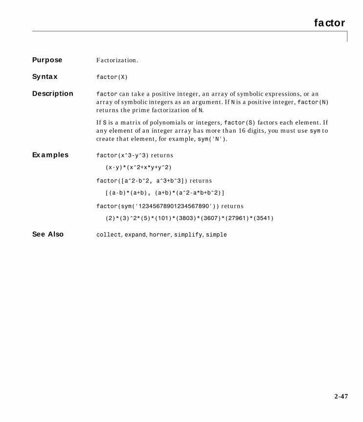
factor
2-47
2factorPurpose Factorization.
Syntax factor(X)
Description factor can take a positive integer, an array of symbolic expressions, or an array of symbolic integers as an argument. If N is a positive integer, factor(N) returns the prime factorization of N.
If S is a matrix of polynomials or integers, factor(S) factors each element. If any element of an integer array has more than 16 digits, you must use sym to create that element, for example, sym('N').
Examples factor(x^3-y^3) returns
(x-y)*(x^2+x*y+y^2)
factor([a^2-b^2, a^3+b^3]) returns
[(a-b)*(a+b), (a+b)*(a^2-a*b+b^2)]
factor(sym('12345678901234567890')) returns
(2)*(3)^2*(5)*(101)*(3803)*(3607)*(27961)*(3541)
See Also collect, expand, horner, simplify, simple
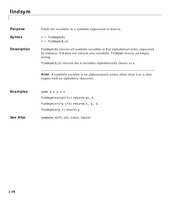
findsym
2-48
2findsymPurpose Finds the variables in a symbolic expression or matrix.
Syntax r = findsym(S)r = findsym(S,n)
Description findsym(S) returns all symbolic variables in S in alphabetical order, separated by commas. If S does not contain any variables, findsym returns an empty string.
findsym(S,n) returns the n variables alphabetically closest to x.
Note A symbolic variable is an alphanumeric name, other than i or j, that begins with an alphabetic character.
Examples syms a x y z t
findsym(sin(pi*t)) returns pi, t.
findsym(x+i*y-j*z) returns x, y, z.
findsym(a+y,1) returns y.
See Also compose, diff, int, limit, taylor
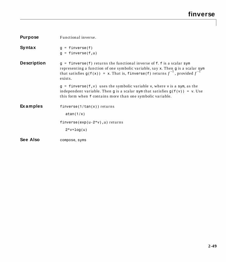
finverse
2-49
2finversePurpose Functional inverse.
Syntax g = finverse(f)g = finverse(f,u)
Description g = finverse(f) returns the functional inverse of f. f is a scalar sym representing a function of one symbolic variable, say x. Then g is a scalar sym that satisfies g(f(x)) = x. That is, finverse(f) returns , provided exists.
g = finverse(f,v) uses the symbolic variable v, where v is a sym, as the independent variable. Then g is a scalar sym that satisfies g(f(v)) = v. Use this form when f contains more than one symbolic variable.
Examples finverse(1/tan(x)) returns
atan(1/x)
finverse(exp(u-2*v),u) returns
2*v+log(u)
See Also compose, syms
f 1– f 1–
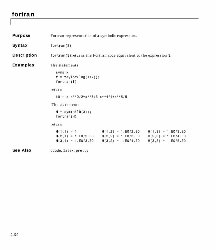
fortran
2-50
2fortranPurpose Fortran representation of a symbolic expression.
Syntax fortran(S)
Description fortran(S)returns the Fortran code equivalent to the expression S.
Examples The statements
syms xf = taylor(log(1+x));fortran(f)
return
t0 = x-x**2/2+x**3/3-x**4/4+x**5/5
The statements
H = sym(hilb(3));fortran(H)
return
H(1,1) = 1 H(1,2) = 1.E0/2.E0 H(1,3) = 1.E0/3.E0H(2,1) = 1.E0/2.E0 H(2,2) = 1.E0/3.E0 H(2,3) = 1.E0/4.E0H(3,1) = 1.E0/3.E0 H(3,2) = 1.E0/4.E0 H(3,3) = 1.E0/5.E0
See Also ccode, latex, pretty
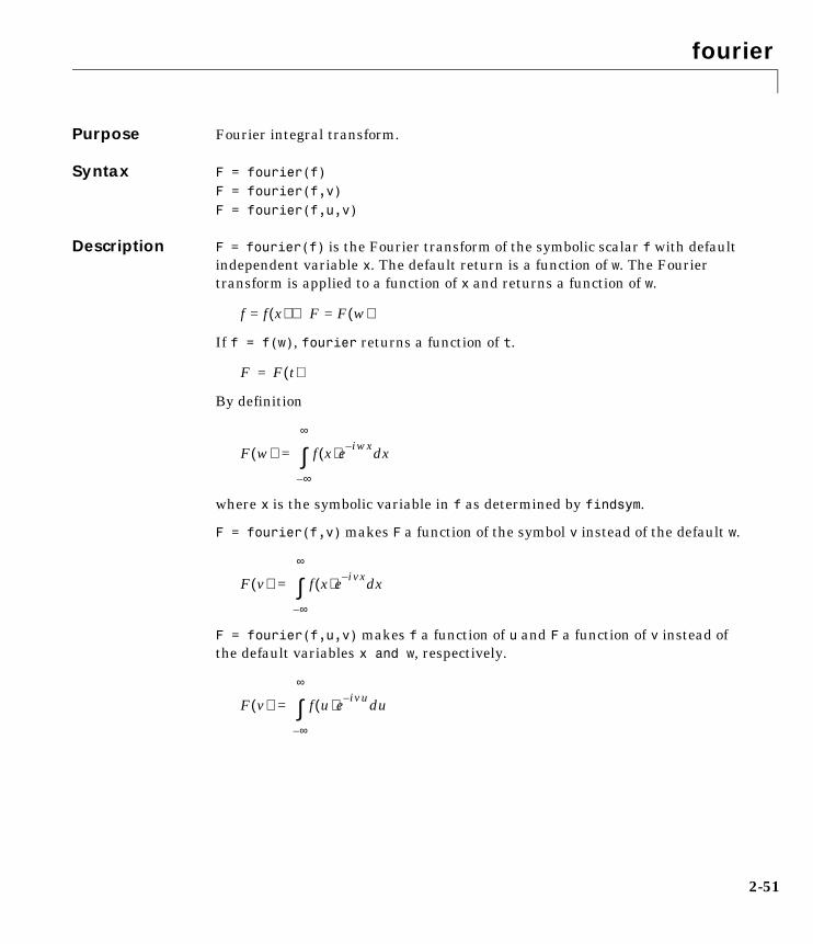
fourier
2-51
2fourierPurpose Fourier integral transform.
Syntax F = fourier(f)F = fourier(f,v)F = fourier(f,u,v)
Description F = fourier(f) is the Fourier transform of the symbolic scalar f with default independent variable x. The default return is a function of w. The Fourier transform is applied to a function of x and returns a function of w.
If f = f(w), fourier returns a function of t.
By definition
where x is the symbolic variable in f as determined by findsym.
F = fourier(f,v) makes F a function of the symbol v instead of the default w.
F = fourier(f,u,v) makes f a function of u and F a function of v instead of the default variables x and w, respectively.
f f x( )= F F w( )=⇒
F F t( )=
F w( ) f x( )e iwx– xd
∞–
∞
∫=
F v( ) f x( )e ivx– xd
∞–
∞
∫=
F v( ) f u( )e ivu– ud
∞–
∞
∫=
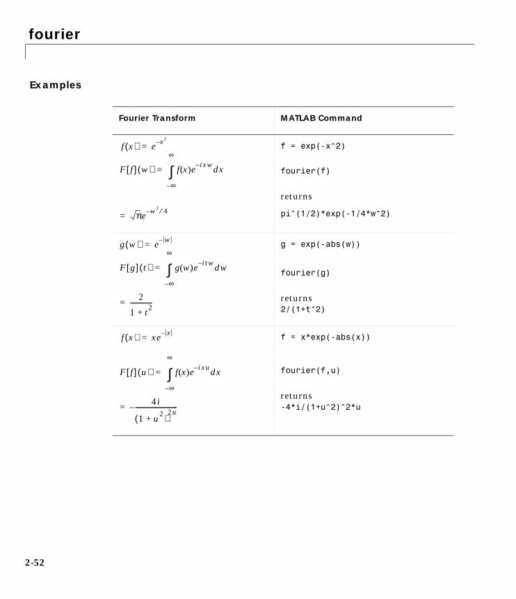
fourier
2-52
Examples
Fourier Transform MATLAB Command
f = exp(-x^2)
fourier(f)
returns
pi^(1/2)*exp(-1/4*w^2)
g = exp(-abs(w))
fourier(g)
returns2/(1+t^2)
f = x*exp(-abs(x))
fourier(f,u)
returns-4*i/(1+u^2)^2*u
f x( ) e x2–=
F f[ ] w( ) f x( )e ixw– xd
∞–
∞
∫=
πe w– 2 4⁄=
g w( ) e w–=
F g[ ] t( ) g w( )e itw– wd
∞–
∞
∫=
2
1 t2+
--------------=
f x( ) xe x–=
F f[ ] u( ) f x( )e ixu– xd
∞–
∞
∫=
4i
1 u2+( )
2u---------------------------–=
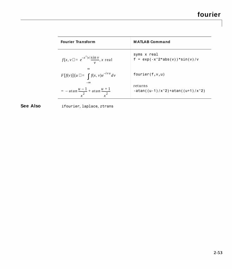
fourier
2-53
See Also ifourier, laplace, ztrans
syms x realf = exp(-x^2*abs(v))*sin(v)/v
fourier(f,v,u)
returns-atan((u-1)/x^2)+atan((u+1)/x^2)
Fourier Transform MATLAB Command
f x v,( ) e x2 v– vsinv
------------ x real,=
F f v( )[ ] u( ) f x v,( )e ivu– vd
∞–
∞
∫=
u 1–
x2-------------atan– u 1+
x2-------------atan+=

funtool
2-54
2funtoolPurpose Function calculator.
Syntax funtool
Description funtool is a visual function calculator that manipulates and displays functions of one variable. At the click of a button, for example, funtool draws a graph representing the sum, product, difference, or ratio of two functions that you specify. funtool includes a function memory that allows you to store functions for later retrieval.
At startup, funtool displays graphs of a pair of functions, f(x) = x andg(x) = 1. The graphs plot the functions over the domain [-2*pi, 2*pi]. funtool also displays a control panel that lets you save, retrieve, redefine, combine, and transform f and g.
Text Fields. The top of the control panel contains a group of editable text fields.
f= Displays a symbolic expression representing f. Edit this field to redefine f.
g= Displays a symbolic expression representing g. Edit this field to redefine g.
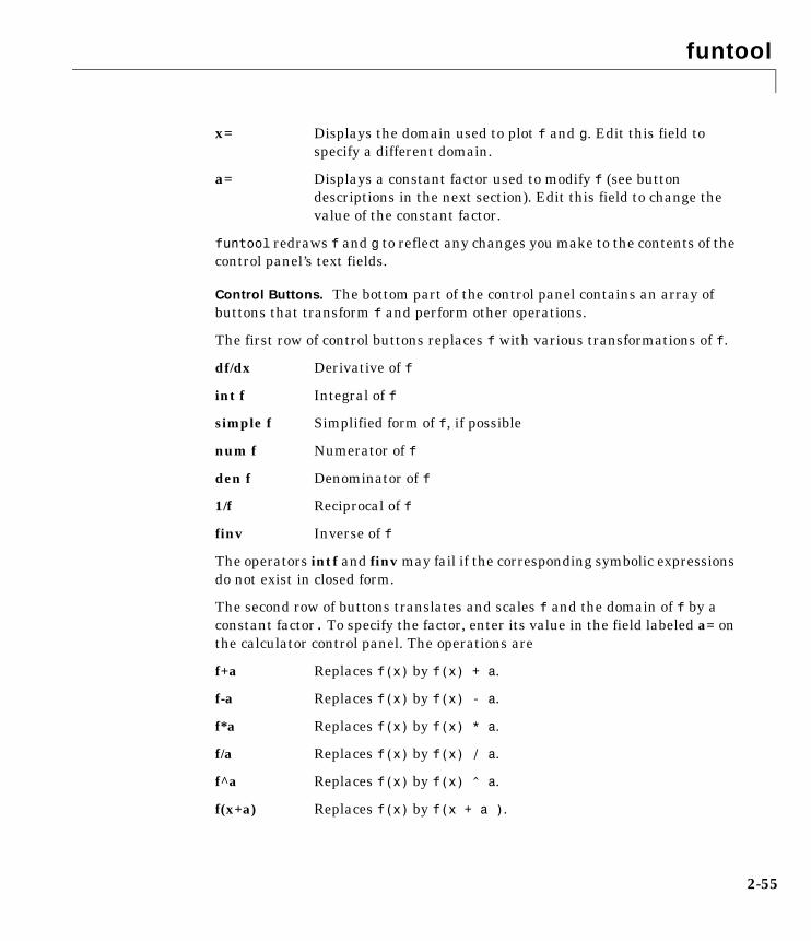
funtool
2-55
x= Displays the domain used to plot f and g. Edit this field to specify a different domain.
a= Displays a constant factor used to modify f (see button descriptions in the next section). Edit this field to change the value of the constant factor.
funtool redraws f and g to reflect any changes you make to the contents of the control panel’s text fields.
Control Buttons. The bottom part of the control panel contains an array of buttons that transform f and perform other operations.
The first row of control buttons replaces f with various transformations of f.
df/dx Derivative of f
int f Integral of f
simple f Simplified form of f, if possible
num f Numerator of f
den f Denominator of f
1/f Reciprocal of f
finv Inverse of f
The operators intf and finv may fail if the corresponding symbolic expressions do not exist in closed form.
The second row of buttons translates and scales f and the domain of f by a constant factor. To specify the factor, enter its value in the field labeled a= on the calculator control panel. The operations are
f+a Replaces f(x) by f(x) + a.
f-a Replaces f(x) by f(x) - a.
f*a Replaces f(x) by f(x) * a.
f/a Replaces f(x) by f(x) / a.
f^a Replaces f(x) by f(x) ^ a.
f(x+a) Replaces f(x) by f(x + a ).
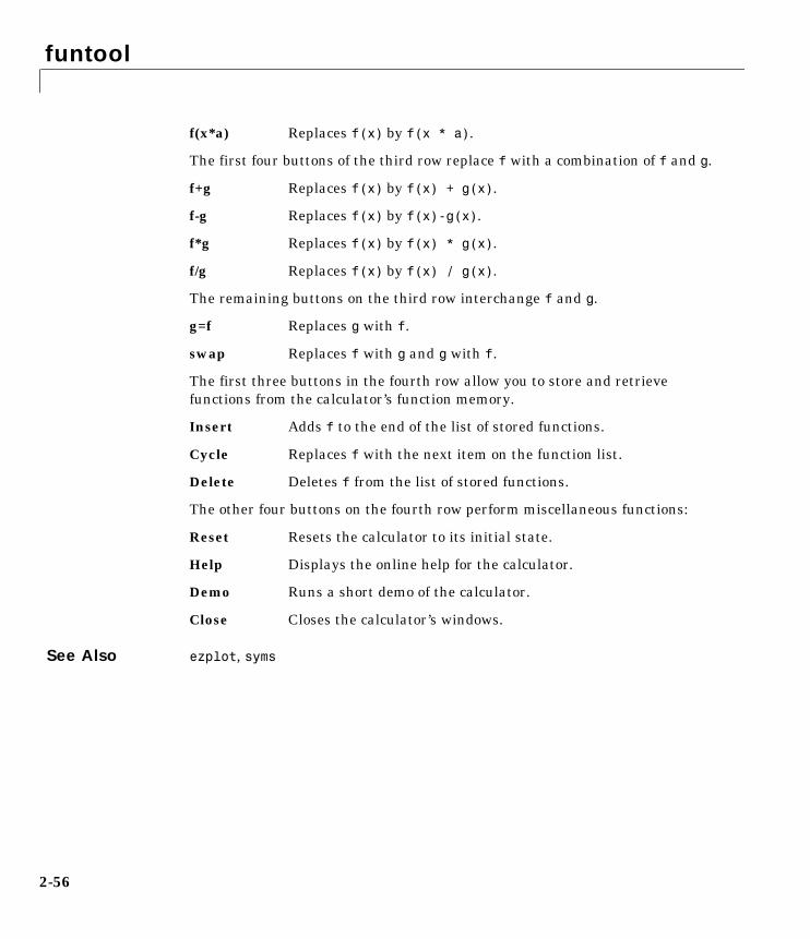
funtool
2-56
f(x*a) Replaces f(x) by f(x * a).
The first four buttons of the third row replace f with a combination of f and g.
f+g Replaces f(x) by f(x) + g(x).
f-g Replaces f(x) by f(x)-g(x).
f*g Replaces f(x) by f(x) * g(x).
f/g Replaces f(x) by f(x) / g(x).
The remaining buttons on the third row interchange f and g.
g=f Replaces g with f.
swap Replaces f with g and g with f.
The first three buttons in the fourth row allow you to store and retrieve functions from the calculator’s function memory.
Insert Adds f to the end of the list of stored functions.
Cycle Replaces f with the next item on the function list.
Delete Deletes f from the list of stored functions.
The other four buttons on the fourth row perform miscellaneous functions:
Reset Resets the calculator to its initial state.
Help Displays the online help for the calculator.
Demo Runs a short demo of the calculator.
Close Closes the calculator’s windows.
See Also ezplot, syms

horner
2-57
2hornerPurpose Horner polynomial representation.
Syntax R = horner(P)
Description Suppose P is a matrix of symbolic polynomials. horner(P) transforms each element of P into its Horner, or nested, representation.
Examples horner(x^3-6*x^2+11*x-6) returns
-6+(11+(-6+x)*x)*x
horner([x^2+x;y^3-2*y]) returns
[ (1+x)*x][(-2+y^2)*y]
See Also expand, factor, simple, simplify, syms
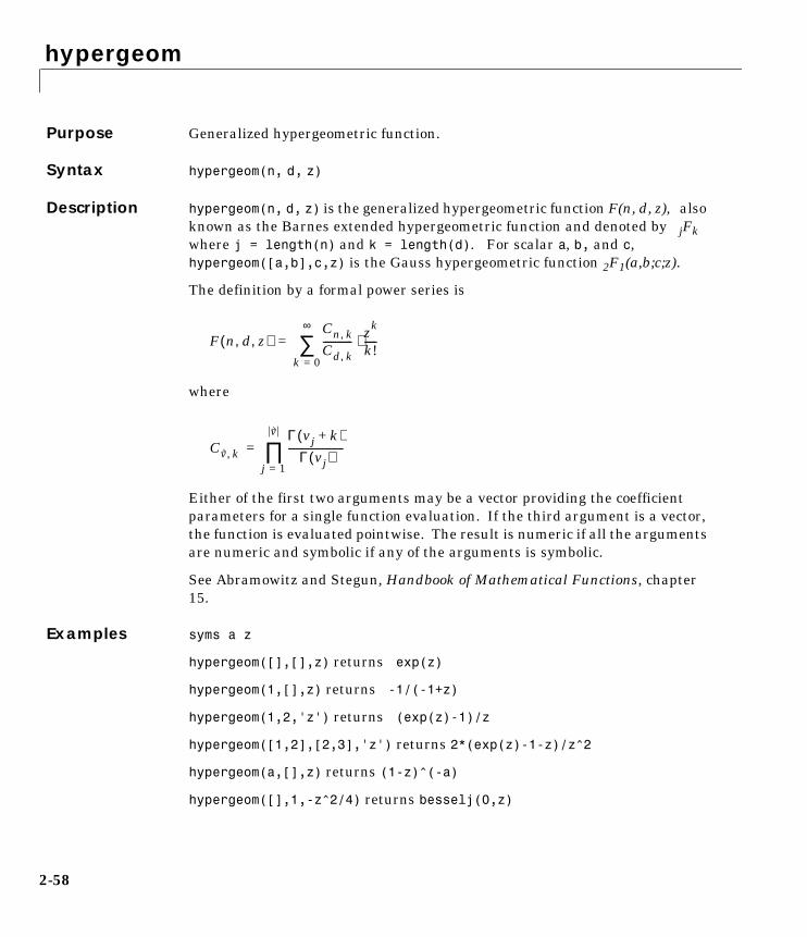
hypergeom
2-58
2hypergeomPurpose Generalized hypergeometric function.
Syntax hypergeom(n, d, z)
Description hypergeom(n, d, z) is the generalized hypergeometric function F(n, d, z), also known as the Barnes extended hypergeometric function and denoted by jFk where j = length(n) and k = length(d). For scalar a, b, and c, hypergeom([a,b],c,z) is the Gauss hypergeometric function 2F1(a,b;c;z).
The definition by a formal power series is
where
Either of the first two arguments may be a vector providing the coefficient parameters for a single function evaluation. If the third argument is a vector, the function is evaluated pointwise. The result is numeric if all the arguments are numeric and symbolic if any of the arguments is symbolic.
See Abramowitz and Stegun, Handbook of Mathematical Functions, chapter 15.
Examples syms a z
hypergeom([],[],z) returns exp(z)
hypergeom(1,[],z) returns -1/(-1+z)
hypergeom(1,2,'z') returns (exp(z)-1)/z
hypergeom([1,2],[2,3],'z') returns 2*(exp(z)-1-z)/z^2
hypergeom(a,[],z) returns (1-z)^(-a)
hypergeom([],1,-z^2/4) returns besselj(0,z)
F n d z, ,( )Cn k,Cd k,------------
zk
k!-----⋅
k 0=
∞
∑=
Cv k,Γ vj k+( )
Γ vj( )-----------------------
j 1=
v
∏=
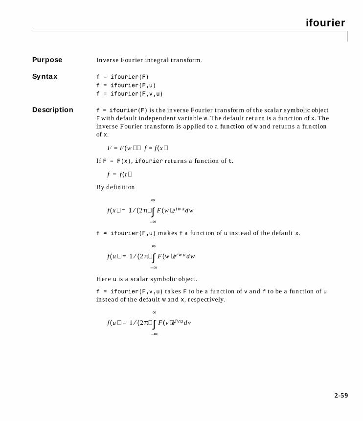
ifourier
2-59
2ifourierPurpose Inverse Fourier integral transform.
Syntax f = ifourier(F)f = ifourier(F,u)f = ifourier(F,v,u)
Description f = ifourier(F) is the inverse Fourier transform of the scalar symbolic object F with default independent variable w. The default return is a function of x. The inverse Fourier transform is applied to a function of w and returns a function of x.
If F = F(x), ifourier returns a function of t.
By definition
f = ifourier(F,u) makes f a function of u instead of the default x.
Here u is a scalar symbolic object.
f = ifourier(F,v,u) takes F to be a function of v and f to be a function of u instead of the default w and x, respectively.
F F w( )= f f x( )=⇒
f f t( )=
f x( ) 1 2π( )⁄ F w( )eiwx wd
∞–
∞
∫=
f u( ) 1 2π( )⁄ F w( )eiwu wd
∞–
∞
∫=
f u( ) 1 2π( )⁄ F v( )eivu vd
∞–
∞
∫=
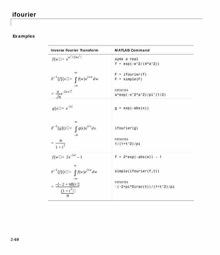
ifourier
2-60
Examples
Inverse Fourier Transform MATLAB Command
syms a realf = exp(-w^2/(4*a^2))
F = ifourier(f)F = simple(F)
returnsa*exp(-x^2*a^2)/pi^(1/2)
g = exp(-abs(x))
ifourier(g)
returns1/(1+t^2)/pi
f = 2*exp(-abs(w)) - 1
simple(ifourier(f,t))
returns-(-2+pi*Dirac(t))/(1+t^2)/pi
f w( ) ew2 4a2( )⁄=
F 1– f[ ] x( ) f w( )eixw wd
∞–
∞
∫=
aπ
-------e ax( )2–=
g x( ) e x–=
F 1– g[ ] t( ) g x( )eitx xd
∞–
∞
∫=
π
1 t2+
--------------=
f w( ) 2e w– 1–=
F 1– f[ ] t( ) f w( )eitw wd
∞–
∞
∫=
2– πδ t( )+( )–
1 t2+( )π
-------------------
------------------------------------=

ifourier
2-61
See Also fourier, ilaplace, iztrans
syms w realf = exp(-w^2*abs(v))*sin(v)/v
ifourier(f,v,t)
returns-1/2*(-atan((t+1)/w^2)+atan((-1+t)/w^2))/pi
Inverse Fourier Transform MATLAB Command
f w v,( ) e w2 v– vsinv
------------ w real,=
F 1– f v( )[ ] t( ) f w v,( )eivt vd
∞–
∞
∫=
12π------ t 1+
w2-----------atan t 1–
w2-----------atan–
=

ilaplace
2-62
2ilaplacePurpose Inverse Laplace transform.
Syntax F = ilaplace(L)F = ilaplace(L,y)F = ilaplace(L,y,x)
Description F = ilaplace(L) is the inverse Laplace transform of the scalar symbolic object L with default independent variable s. The default return is a function of t. The inverse Laplace transform is applied to a function of s and returns a function of t.
If L = L(t), ilaplace returns a function of x.
By definition
where c is a real number selected so that all singularities of L(s) are to the left of the line s = c, i.
F = ilaplace(L,y) makes F a function of y instead of the default t.
Here y is a scalar symbolic object.
F = ilaplace(L,y,x) takes F to be a function of x and L a function of y instead of the default variables t and s, respectively.
L L s( )= F F t( )=⇒
F F x( )=
F t( ) L s( )est sd
c i∞–
c i∞+
∫=
F y( ) L y( )esy sd
c i∞–
c i∞+
∫=
F x( ) L y( )exy yd
c i∞–
c i∞+
∫=
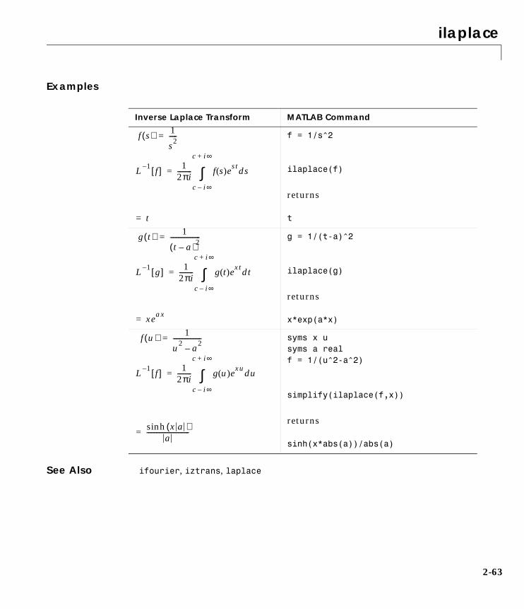
ilaplace
2-63
Examples
See Also ifourier, iztrans, laplace
Inverse Laplace Transform MATLAB Command
f = 1/s^2
ilaplace(f)
returns
t
g = 1/(t-a)^2
ilaplace(g)
returns
x*exp(a*x)
syms x usyms a realf = 1/(u^2-a^2)
simplify(ilaplace(f,x))
returns
sinh(x*abs(a))/abs(a)
f s( ) 1
s2-----=
L 1– f[ ] 12πi--------- f s( )est sd
c i∞–
c i∞+
∫=
t=
g t( ) 1
t a–( )2-------------------=
L 1– g[ ] 12πi--------- g t( )ext td
c i∞–
c i∞+
∫=
xeax=
f u( ) 1
u2 a2–
------------------=
L 1– f[ ] 12πi--------- g u( )exu ud
c i∞–
c i∞+
∫=
x a( )sinha
---------------------------=
imag
2-64
2imagPurpose Symbolic imaginary part.
Syntax imag(Z)
Description imag(Z) is the imaginary part of a symbolic Z.
See Also conj, real

int
2-65
2intPurpose Integrate.
Syntax R = int(S)R = int(S,v)R = int(S,a,b)R = int(S,v,a,b)
Description int(S) returns the indefinite integral of S with respect to its symbolic variable as defined by findsym.
int(S,v) returns the indefinite integral of S with respect to the symbolic scalar variable v.
int(S,a,b) returns the definite integral from a to b of each element of S with respect to each element’s default symbolic variable. a and b are symbolic or double scalars.
int(S,v,a,b) returns the definite integral of S with respect to v from a to b.
Examples int(-2*x/(1+x^2)^2) returns
1/(1+x^2)
int(x/(1+z^2),z) returns
x*atan(z)
int(x*log(1+x),0,1) returns
1/4
int(2*x, sin(t), 1) returns
1-sin(t)^2
int([exp(t),exp(alpha*t)]) returns
[exp(t), 1/alpha*exp(alpha*t)]
See Also diff, symsum
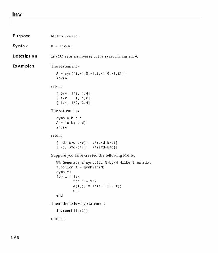
inv
2-66
2invPurpose Matrix inverse.
Syntax R = inv(A)
Description inv(A) returns inverse of the symbolic matrix A.
Examples The statements
A = sym([2,-1,0;-1,2,-1;0,-1,2]);inv(A)
return
[ 3/4, 1/2, 1/4][ 1/2, 1, 1/2][ 1/4, 1/2, 3/4]
The statements
syms a b c dA = [a b; c d]inv(A)
return
[ d/(a*d-b*c), -b/(a*d-b*c)][ -c/(a*d-b*c), a/(a*d-b*c)]
Suppose you have created the following M-file.
%% Generate a symbolic N-by-N Hilbert matrix.function A = genhilb(N)syms t;for i = 1:N for j = 1:N A(i,j) = 1/(i + j - t); endend
Then, the following statement
inv(genhilb(2))
returns
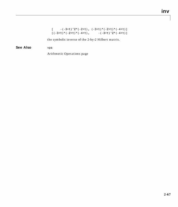
inv
2-67
[ -(-3+t)^2*(-2+t), (-3+t)*(-2+t)*(-4+t)] [(-3+t)*(-2+t)*(-4+t), -(-3+t)^2*(-4+t)]
the symbolic inverse of the 2-by-2 Hilbert matrix.
See Also vpa
Arithmetic Operations page

iztrans
2-68
2iztransPurpose Inverse z-transform.
Syntax f = iztrans(F)f = iztrans(F,k)f = iztrans(F,w,k)
Description f = iztrans(F) is the inverse z-transform of the scalar symbolic object F with default independent variable z. The default return is a function of n.
where R is a positive number chosen so that the function F(z) is analytic on and outside the circle |z| = R.
If F = F(n), iztrans returns a function of k.
f = iztrans(F,k) makes f a function of k instead of the default n. Here k is a scalar symbolic object.
f = iztrans(F,w,k) takes F to be a function of w instead of the default findsym(F) and returns a function of k.
Examples
f n( ) 12πi--------- F z( )zn 1– z n 1 2 …, ,=,d
z R=∫°=
f f k( )=
F F w( )= f f k( )=⇒
Inverse Z-Transform MATLAB Operation
f = 2*z/(z-2)^2
iztrans(f)
returns
2^n*n
f z( ) 2z
z 2–( )2-------------------=
Z 1– f[ ] 12πi--------- f s( )zn 1– dz
z R=∫°=
n2n=
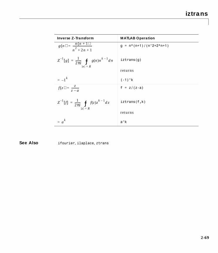
iztrans
2-69
See Also ifourier, ilaplace, ztrans
g = n*(n+1)/(n^2+2*n+1)
iztrans(g)
returns
(-1)^k
f = z/(z-a)
iztrans(f,k)
returns
a^k
Inverse Z-Transform MATLAB Operation
g n( ) n n 1+( )
n2 2n 1+ +------------------------------=
Z 1– g[ ] 12πi--------- g n( )nk 1– dn
n R=∫°=
1–k
=
f z( ) zz a–------------=
Z 1– f[ ] 12πi--------- f z( )zk 1– dz
z R=∫°=
ak=

jacobian
2-70
2jacobianPurpose Jacobian matrix.
Syntax R = jacobian(w,v)
Description jacobian(w,v) computes the Jacobian of w with respect to v. w is a symbolic scalar expression or a symbolic column vector. v is a symbolic row vector. The (i,j)-th entry of the result is .
Examples The statements
w = [x*y*z; y; x+z];v = [x,y,z]; R = jacobian(w,v)b = jacobian(x+z, v)
return
R =[y*z, x*z, x*y][ 0, 1, 0][ 1, 0, 1]
b =[1, 0, 1]
See Also diff
∂w i( ) ∂v j( )⁄
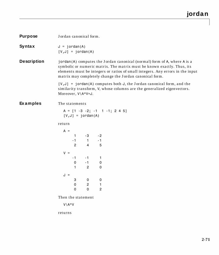
jordan
2-71
2jordanPurpose Jordan canonical form.
Syntax J = jordan(A)[V,J] = jordan(A)
Description jordan(A) computes the Jordan canonical (normal) form of A, where A is a symbolic or numeric matrix. The matrix must be known exactly. Thus, its elements must be integers or ratios of small integers. Any errors in the input matrix may completely change the Jordan canonical form.
[V,J] = jordan(A) computes both J, the Jordan canonical form, and the similarity transform, V, whose columns are the generalized eigenvectors. Moreover, V\A*V=J.
Examples The statements
A = [1 -3 -2; -1 1 -1; 2 4 5][V,J] = jordan(A)
return
A = 1 -3 -2 -1 1 -1 2 4 5
V = -1 -1 1 0 -1 0 1 2 0
J = 3 0 0 0 2 1 0 0 2
Then the statement
V\A*V
returns
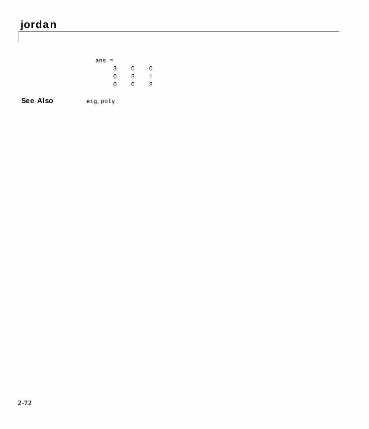
jordan
2-72
ans = 3 0 0 0 2 1 0 0 2
See Also eig, poly
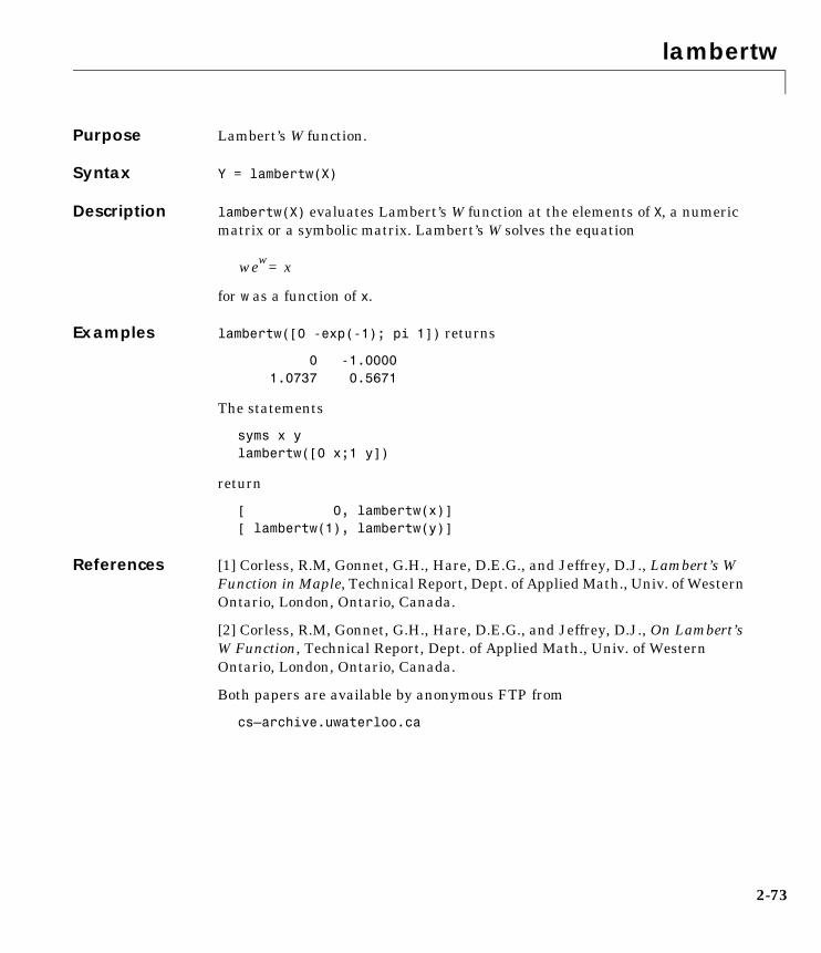
lambertw
2-73
2lambertwPurpose Lambert’s W function.
Syntax Y = lambertw(X)
Description lambertw(X) evaluates Lambert’s W function at the elements of X, a numeric matrix or a symbolic matrix. Lambert’s W solves the equation
for w as a function of x.
Examples lambertw([0 -exp(-1); pi 1]) returns
0 -1.0000 1.0737 0.5671
The statements
syms x ylambertw([0 x;1 y])
return
[ 0, lambertw(x)][ lambertw(1), lambertw(y)]
References [1] Corless, R.M, Gonnet, G.H., Hare, D.E.G., and Jeffrey, D.J., Lambert’s W Function in Maple, Technical Report, Dept. of Applied Math., Univ. of Western Ontario, London, Ontario, Canada.
[2] Corless, R.M, Gonnet, G.H., Hare, D.E.G., and Jeffrey, D.J., On Lambert’s W Function, Technical Report, Dept. of Applied Math., Univ. of Western Ontario, London, Ontario, Canada.
Both papers are available by anonymous FTP from
cs–archive.uwaterloo.ca
wew x=
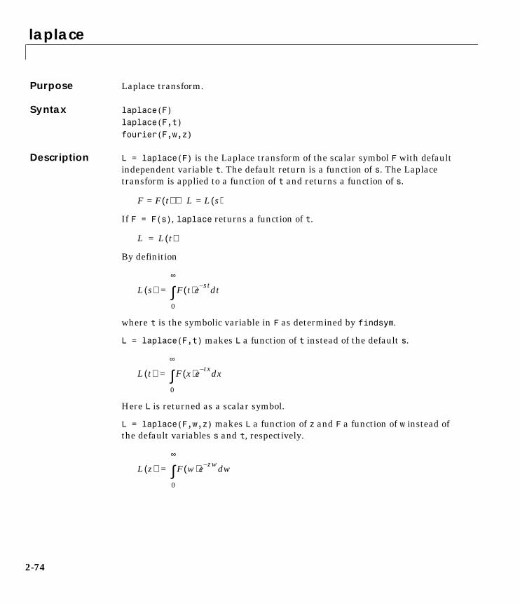
laplace
2-74
2laplacePurpose Laplace transform.
Syntax laplace(F)laplace(F,t)fourier(F,w,z)
Description L = laplace(F) is the Laplace transform of the scalar symbol F with default independent variable t. The default return is a function of s. The Laplace transform is applied to a function of t and returns a function of s.
If F = F(s), laplace returns a function of t.
By definition
where t is the symbolic variable in F as determined by findsym.
L = laplace(F,t) makes L a function of t instead of the default s.
Here L is returned as a scalar symbol.
L = laplace(F,w,z) makes L a function of z and F a function of w instead of the default variables s and t, respectively.
F F t( )= L L s( )=⇒
L L t( )=
L s( ) F t( )e st– td
0
∞
∫=
L t( ) F x( )e tx– xd
0
∞
∫=
L z( ) F w( )e zw– wd
0
∞
∫=
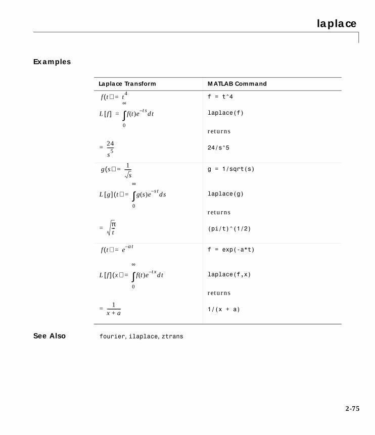
laplace
2-75
Examples
See Also fourier, ilaplace, ztrans
Laplace Transform MATLAB Command
f = t^4
laplace(f)
returns
24/s^5
g = 1/sqrt(s)
laplace(g)
returns
(pi/t)^(1/2)
f = exp(-a*t)
laplace(f,x)
returns
1/(x + a)
f t( ) t4=
L f[ ] f t( )e ts– td
0
∞
∫=
24
s5------=
g s( ) 1s
------=
L g[ ] t( ) g s( )e st– sd
0
∞
∫=
πt---=
f t( ) e at–=
L f[ ] x( ) f t( )e tx– td
0
∞
∫=
1x a+------------=
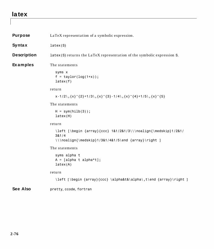
latex
2-76
2latexPurpose LaTeX representation of a symbolic expression.
Syntax latex(S)
Description latex(S) returns the LaTeX representation of the symbolic expression S.
Examples The statements
syms xf = taylor(log(1+x));latex(f)
return
x-1/2\,{x}^{2}+1/3\,{x}^{3}-1/4\,{x}^{4}+1/5\,{x}^{5}
The statements
H = sym(hilb(3));latex(H)
return
\left [\begin {array}{ccc} 1&1/2&1/3\\\noalign{\medskip}1/2&1/3&1/4\\\noalign{\medskip}1/3&1/4&1/5\end {array}\right ]
The statements
syms alpha tA = [alpha t alpha*t];latex(A)
return
\left [\begin {array}{ccc} \alpha&t&\alpha\,t\end {array}\right ]
See Also pretty, ccode, fortran
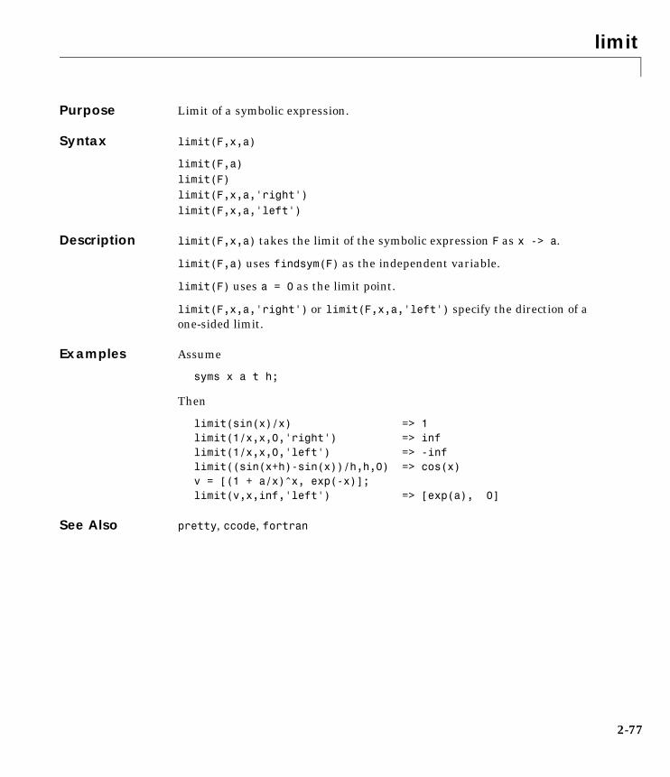
limit
2-77
2limitPurpose Limit of a symbolic expression.
Syntax limit(F,x,a)
limit(F,a)limit(F)limit(F,x,a,'right')limit(F,x,a,'left')
Description limit(F,x,a) takes the limit of the symbolic expression F as x -> a.
limit(F,a) uses findsym(F) as the independent variable.
limit(F) uses a = 0 as the limit point.
limit(F,x,a,'right') or limit(F,x,a,'left') specify the direction of a one-sided limit.
Examples Assume
syms x a t h;
Then
limit(sin(x)/x) => 1limit(1/x,x,0,'right') => inflimit(1/x,x,0,'left') => -inflimit((sin(x+h)-sin(x))/h,h,0) => cos(x)v = [(1 + a/x)^x, exp(-x)];limit(v,x,inf,'left') => [exp(a), 0]
See Also pretty, ccode, fortran
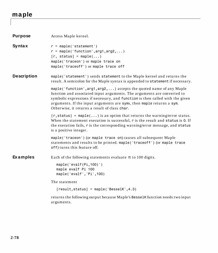
maple
2-78
2maplePurpose Access Maple kernel.
Syntax r = maple('statement')r = maple('function',arg1,arg2,...)[r, status] = maple(...)maple('traceon') or maple trace onmaple('traceoff') or maple trace off
Description maple('statement') sends statement to the Maple kernel and returns the result. A semicolon for the Maple syntax is appended to statement if necessary.
maple('function',arg1,arg2,...) accepts the quoted name of any Maple function and associated input arguments. The arguments are converted to symbolic expressions if necessary, and function is then called with the given arguments. If the input arguments are syms, then maple returns a sym. Otherwise, it returns a result of class char.
[r,status] = maple(...) is an option that returns the warning/error status. When the statement execution is successful, r is the result and status is 0. If the execution fails, r is the corresponding warning/error message, and status is a positive integer.
maple('traceon') (or maple trace on) causes all subsequent Maple statements and results to be printed. maple('traceoff') (or maple trace off) turns this feature off.
Examples Each of the following statements evaluate to 100 digits.
maple('evalf(Pi,100)')maple evalf Pi 100maple('evalf','Pi',100)
The statement
[result,status] = maple('BesselK',4.3)
returns the following output because Maple’s BesselK function needs two input arguments.
π

maple
2-79
result =Error, (in BesselK) expecting 2 arguments, got 1status =2
The traceon command shows how Symbolic Math Toolbox commands interact with Maple. For example, the statements
syms xv = [x^2-1;x^2-4]maple traceon % or maple trace onw = factor(v)
return
v =[ x^2-1][ x^2-4] statement: map(ifactor,array([[x^2-1],[x^2-4]]));result: Error, (in ifactor) invalid argumentsstatement: map(factor,array([[x^2-1],[x^2-4]]));result: matrix([[(x-1)*(x+1)], [(x-2)*(x+2)]]) w = [ (x-1)*(x+1)][ (x-2)*(x+2)]
This example reveals that the factor statement first invokes Maple’s integer factor (ifactor) statement to determine whether the argument is a factorable integer. If Maple’s integer factor statement returns an error, the Symbolic Math Toolbox factor statement then invokes Maple’s expression factoring statement.
See Also mhelp, procread
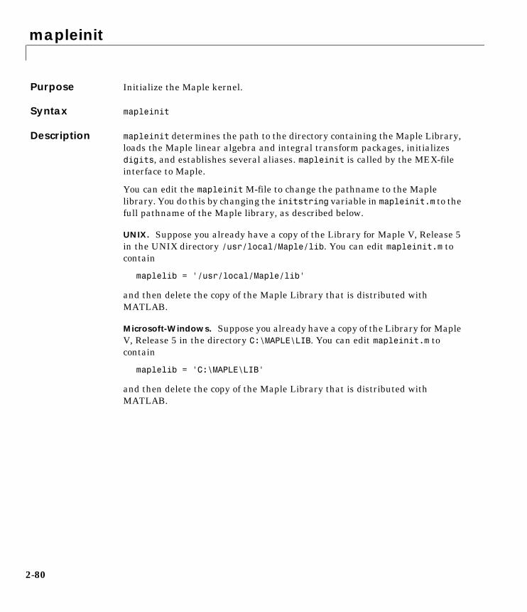
mapleinit
2-80
2mapleinitPurpose Initialize the Maple kernel.
Syntax mapleinit
Description mapleinit determines the path to the directory containing the Maple Library, loads the Maple linear algebra and integral transform packages, initializes digits, and establishes several aliases. mapleinit is called by the MEX-file interface to Maple.
You can edit the mapleinit M-file to change the pathname to the Maple library. You do this by changing the initstring variable in mapleinit.m to the full pathname of the Maple library, as described below.
UNIX. Suppose you already have a copy of the Library for Maple V, Release 5 in the UNIX directory /usr/local/Maple/lib. You can edit mapleinit.m to contain
maplelib = '/usr/local/Maple/lib'
and then delete the copy of the Maple Library that is distributed with MATLAB.
Microsoft-Windows. Suppose you already have a copy of the Library for Maple V, Release 5 in the directory C:\MAPLE\LIB. You can edit mapleinit.m to contain
maplelib = 'C:\MAPLE\LIB'
and then delete the copy of the Maple Library that is distributed with MATLAB.
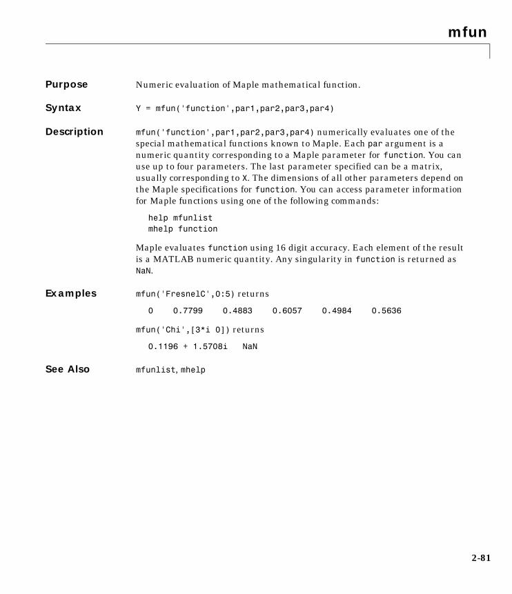
mfun
2-81
2mfunPurpose Numeric evaluation of Maple mathematical function.
Syntax Y = mfun('function',par1,par2,par3,par4)
Description mfun('function',par1,par2,par3,par4) numerically evaluates one of the special mathematical functions known to Maple. Each par argument is a numeric quantity corresponding to a Maple parameter for function. You can use up to four parameters. The last parameter specified can be a matrix, usually corresponding to X. The dimensions of all other parameters depend on the Maple specifications for function. You can access parameter information for Maple functions using one of the following commands:
help mfunlistmhelp function
Maple evaluates function using 16 digit accuracy. Each element of the result is a MATLAB numeric quantity. Any singularity in function is returned as NaN.
Examples mfun('FresnelC',0:5) returns
0 0.7799 0.4883 0.6057 0.4984 0.5636
mfun('Chi',[3*i 0]) returns
0.1196 + 1.5708i NaN
See Also mfunlist, mhelp
mfunlist
2-82
2mfunlistPurpose List special functions for use with mfun.
Syntax mfunlist % help mfunlist on the Macintosh
Description mfunlist lists the special mathematical functions for use with the mfun function. The following tables describe these special functions.
You can access more detailed descriptions by typing
mhelp function
Limitations In general, the accuracy of a function will be lower near its roots and when its arguments are relatively large.
Runtime depends on the specific function and its parameters. In general, calculations are slower than standard MATLAB calculations.
See Also mfun, mhelp
References [1] Abramowitz, M. and Stegun, I.A., Handbook of Mathematical Functions , Dover Publications, 1965.
Table Conventions
The following conventions are used in Table 2-1, MFUN Special Functions, unless otherwise indicated in the Arguments column.
x, y real argument
z , z1, z2 complex argument
m , n integer argument
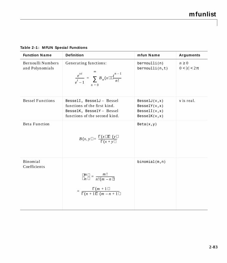
mfunlist
2-83
Table 2-1: MFUN Special Functions
Function Name Definition mfun Name Arguments
Bernoulli Numbers and Polynomials
Generating functions: bernoulli(n)bernoulli(n,t)
Bessel Functions BesselI, BesselJ – Bessel functions of the first kind.BesselK, BesselY – Bessel functions of the second kind.
BesselJ(v,x)BesselY(v,x)BesselI(v,x)BesselK(v,x)
v is real.
Beta Function Beta(x,y)
Binomial Coefficients
binomial(m,n)
ext
et 1–------------- Bn x( ) tn 1–
n!------------⋅
n 0=
∞
∑=
n 0≥0 t 2π< <
B x y,( ) Γ x( ) Γ y( )⋅Γ x y+( )
----------------------------=
mn
m!n! m n–( )!---------------------------=
Γ m 1+( )Γ n 1+( )Γ m n 1+–( )--------------------------------------------------------=
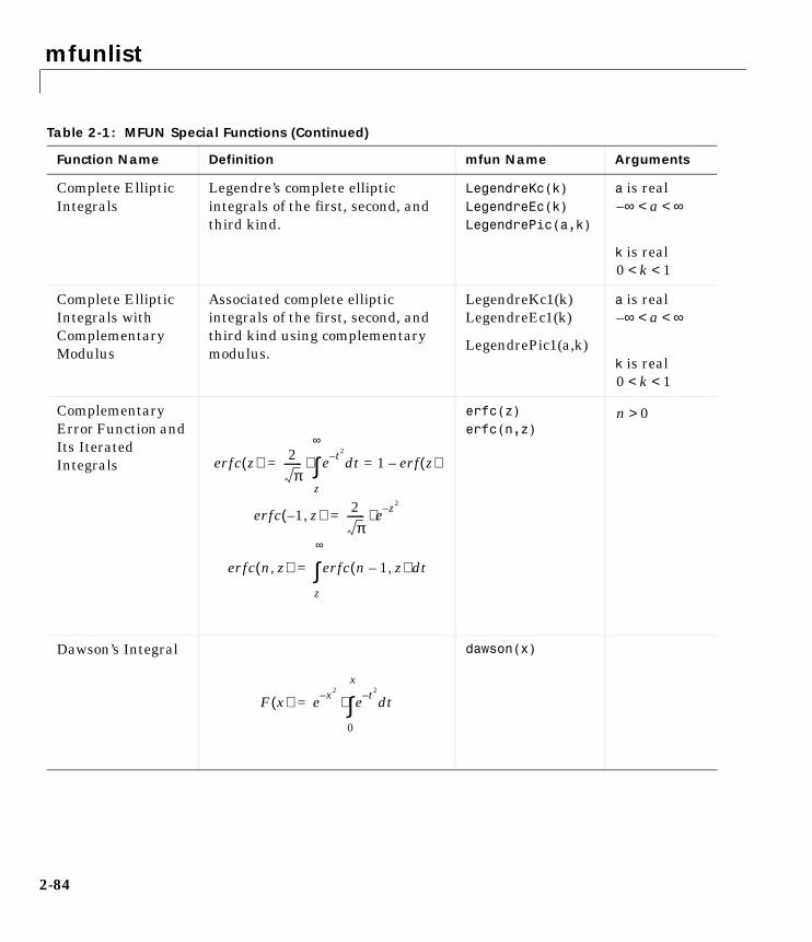
mfunlist
2-84
Complete Elliptic Integrals
Legendre’s complete elliptic integrals of the first, second, and third kind.
LegendreKc(k)LegendreEc(k)LegendrePic(a,k)
a is real
k is real
Complete Elliptic Integrals with Complementary Modulus
Associated complete elliptic integrals of the first, second, and third kind using complementary modulus.
LegendreKc1(k)LegendreEc1(k)
LegendrePic1(a,k)
a is real
k is real
Complementary Error Function and Its Iterated Integrals
erfc(z)erfc(n,z)
Dawson’s Integral dawson(x)
Table 2-1: MFUN Special Functions (Continued)
Function Name Definition mfun Name Arguments
∞– a ∞< <
0 k 1< <
∞– a ∞< <
0 k 1< <
erfc z( ) 2π
------- e t– 2
t 1 erf z( )–=d
z
∞
∫⋅=
erfc 1 z,–( ) 2π
------- e z– 2
⋅=
erfc n z,( ) erfc n 1– z,( ) td
z
∞
∫=
n 0>
F x( ) e x2– e t2– td
0
x
∫⋅=

mfunlist
2-85
Digamma Function Psi(x)
Dilogarithm Integral
dilog(x)
Error Function erf(z)
Euler Numbers and Polynomials
Generating function for Euler numbers:
euler(n)euler(n,z)
Table 2-1: MFUN Special Functions (Continued)
Function Name Definition mfun Name Arguments
ψ x( )xd
d Γ x( )( )ln Γ′ x( )Γ x( )-------------= =
f x( ) t( )ln1 t–------------- td
1
x
∫=
x 1>
erf z( ) 2π
------- e t– 2
td
0
z
∫=
1ch t( )-------------- En
tn
n!-----
n 0=
∞
∑=
n 0≥
t π2---<
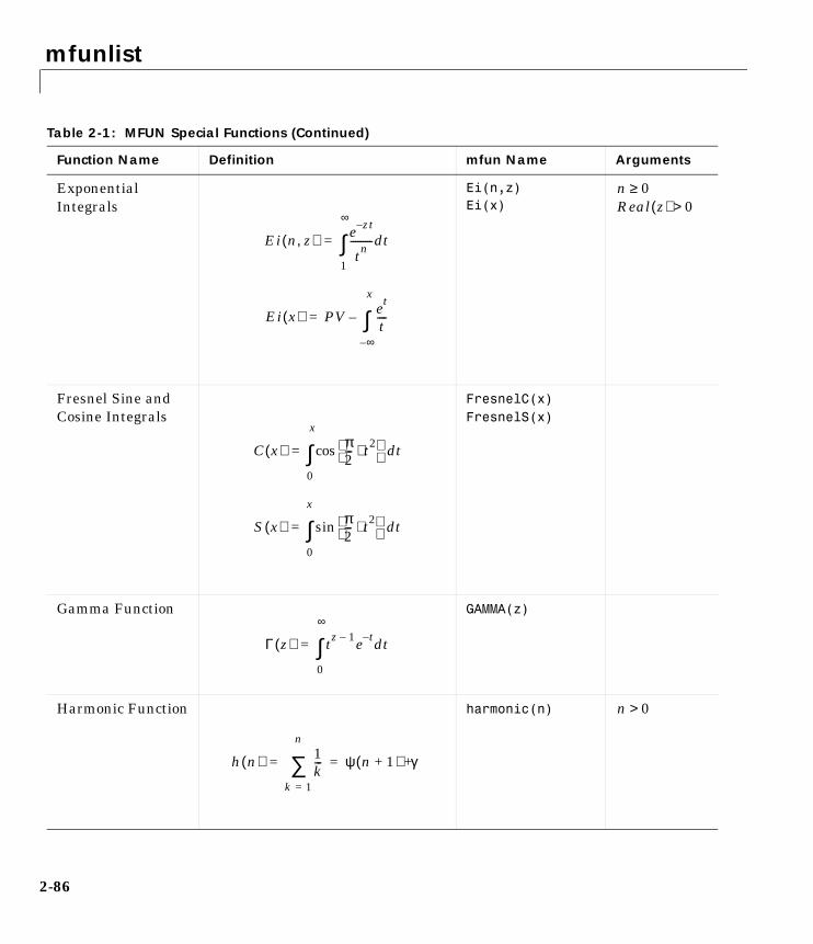
mfunlist
2-86
Exponential Integrals
Ei(n,z)Ei(x)
Fresnel Sine and Cosine Integrals
FresnelC(x)FresnelS(x)
Gamma Function GAMMA(z)
Harmonic Function harmonic(n)
Table 2-1: MFUN Special Functions (Continued)
Function Name Definition mfun Name Arguments
Ei n z,( ) e zt–
tn--------- td
1
∞
∫=
Ei x( ) PV et
t----
∞–
x
∫–=
n 0≥Real z( ) 0>
C x( ) π2--- t2⋅
cos td
0
x
∫=
S x( ) π2--- t2⋅
sin td
0
x
∫=
Γ z( ) tz 1– e t– td
0
∞
∫=
h n( ) 1k---
k 1=
n
∑ ψ n 1+( ) γ+= =
n 0>

mfunlist
2-87
Hyperbolic Sine and Cosine Integrals
Shi(z)Chi(z)
(Generalized) Hypergeometric Function
where j and m are the number of terms in n and d, respectively.
hypergeom(n,d,x)
wheren = [n1,n2,...]d = [d1,d2,...]
n1,n2,... are real. d1,d2,... are real and non-negative.
Incomplete Elliptic Integrals
Legendre’s incomplete elliptic integrals of the first, second, and third kind.
LegendreF(x,k)
LegendreE(x,k)
LegendrePi(x,a,k)
a is real
k is real
Table 2-1: MFUN Special Functions (Continued)
Function Name Definition mfun Name Arguments
Shi z( ) t( )sinht
------------------- td
0
z
∫=
Chi z( ) γ z( )ln t( )cosh 1–t
----------------------------- td
0
z
∫+ +=
F n d z, ,( )
Γ ni k+( )Γ ni( )
------------------------ zk⋅
i 1=
j
∏
Γ di k+( )Γ di( )
------------------------ k!⋅
i 1=
m
∏---------------------------------------------
k 0=
∞
∑=
0 x ∞≤<
∞– a ∞< <
0 k 1< <

mfunlist
2-88
Incomplete Gamma Function
GAMMA(z1,z2)
Logarithm of the Gamma Function
lnGAMMA(z)
Logarithmic Integral
Li(x)
Table 2-1: MFUN Special Functions (Continued)
Function Name Definition mfun Name Arguments
Γ a z,( ) e t– ta 1–⋅ td
z
∞
∫=
Γ z( )ln Γ z( )( )ln=
Li x( ) PV tdtln
--------
0
x
∫
Ei xln( )= =
x 1>
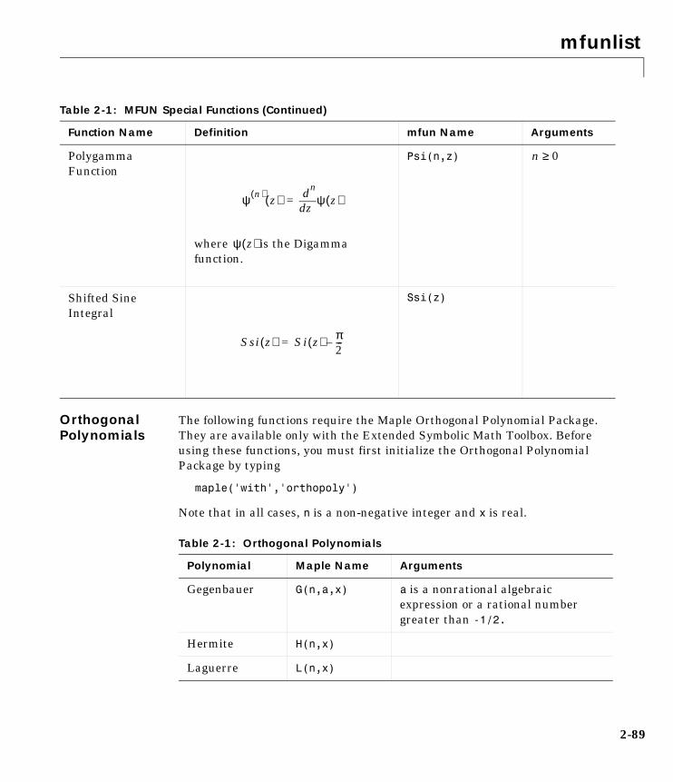
mfunlist
2-89
Orthogonal Polynomials
The following functions require the Maple Orthogonal Polynomial Package. They are available only with the Extended Symbolic Math Toolbox. Before using these functions, you must first initialize the Orthogonal Polynomial Package by typing
maple('with','orthopoly')
Note that in all cases, n is a non-negative integer and x is real.
Polygamma Function
where is the Digamma function.
Psi(n,z)
Shifted Sine Integral
Ssi(z)
Table 2-1: MFUN Special Functions (Continued)
Function Name Definition mfun Name Arguments
ψ n( ) z( )z
n
dd ψ z( )=
ψ z( )
n 0≥
Ssi z( ) Si z( ) π2---–=
Table 2-1: Orthogonal Polynomials
Polynomial Maple Name Arguments
Gegenbauer G(n,a,x) a is a nonrational algebraic expression or a rational number greater than -1/2.
Hermite H(n,x)
Laguerre L(n,x)
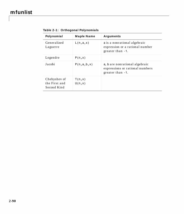
mfunlist
2-90
Generalized Laguerre
L(n,a,x) a is a nonrational algebraic expression or a rational number greater than -1.
Legendre P(n,x)
Jacobi P(n,a,b,x) a, b are nonrational algebraic expressions or rational numbers greater than -1.
Chebyshev of the First and Second Kind
T(n,x)U(n,x)
Table 2-1: Orthogonal Polynomials
Polynomial Maple Name Arguments
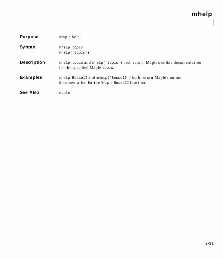
mhelp
2-91
2mhelpPurpose Maple help.
Syntax mhelp topicmhelp('topic')
Description mhelp topic and mhelp('topic') both return Maple’s online documentation for the specified Maple topic.
Examples mhelp BesselI and mhelp('BesselI') both return Maple’s online documentation for the Maple BesselI function.
See Also maple
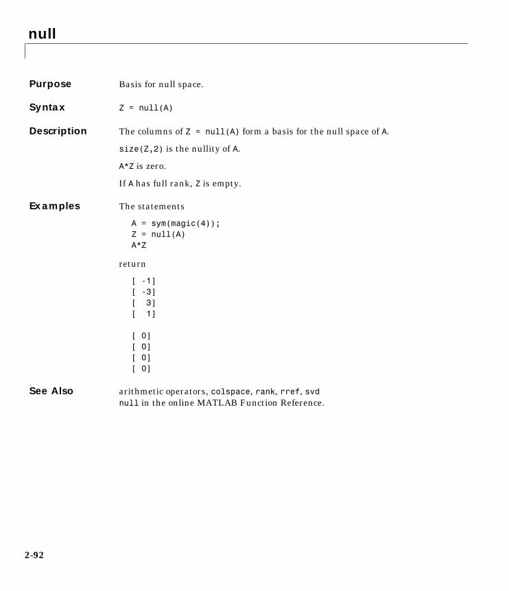
null
2-92
2nullPurpose Basis for null space.
Syntax Z = null(A)
Description The columns of Z = null(A) form a basis for the null space of A.
size(Z,2) is the nullity of A.
A*Z is zero.
If A has full rank, Z is empty.
Examples The statements
A = sym(magic(4));Z = null(A)A*Z
return
[ -1][ -3][ 3][ 1]
[ 0][ 0][ 0][ 0]
See Also arithmetic operators, colspace, rank, rref, svd null in the online MATLAB Function Reference.

numden
2-93
2numdenPurpose Numerator and denominator.
Syntax [N,D] = numden(A)
Description [N,D] = numden(A) converts each element of A to a rational form where the numerator and denominator are relatively prime polynomials with integer coefficients. A is a symbolic or a numeric matrix. N is the symbolic matrix of numerators, and D is the symbolic matrix of denominators.
Examples [n,d] = numden(sym(4/5)) returns n = 4 and d = 5.
[n,d] = numden(x/y + y/x) returns
n = x^2+y^2
d = y*x
The statements
A = [a, 1/b][n,d] = numden(A)
return
A =[a, 1/b] n =[a, 1]
d =[1, b]
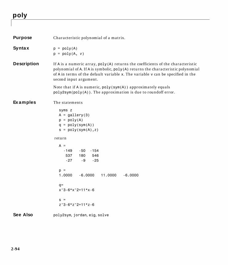
poly
2-94
2polyPurpose Characteristic polynomial of a matrix.
Syntax p = poly(A)p = poly(A, v)
Description If A is a numeric array, poly(A) returns the coefficients of the characteristic polynomial of A. If A is symbolic, poly(A) returns the characteristic polynomial of A in terms of the default variable x. The variable v can be specified in the second input argument.
Note that if A is numeric, poly(sym(A)) approximately equals poly2sym(poly(A)). The approximation is due to roundoff error.
Examples The statements
syms zA = gallery(3) p = poly(A)q = poly(sym(A))s = poly(sym(A),z)
return
A = -149 -50 -154 537 180 546 -27 -9 -25
p = 1.0000 -6.0000 11.0000 -6.0000
q=x^3-6*x^2+11*x-6
s =z^3-6*z^2+11*z-6
See Also poly2sym, jordan, eig, solve
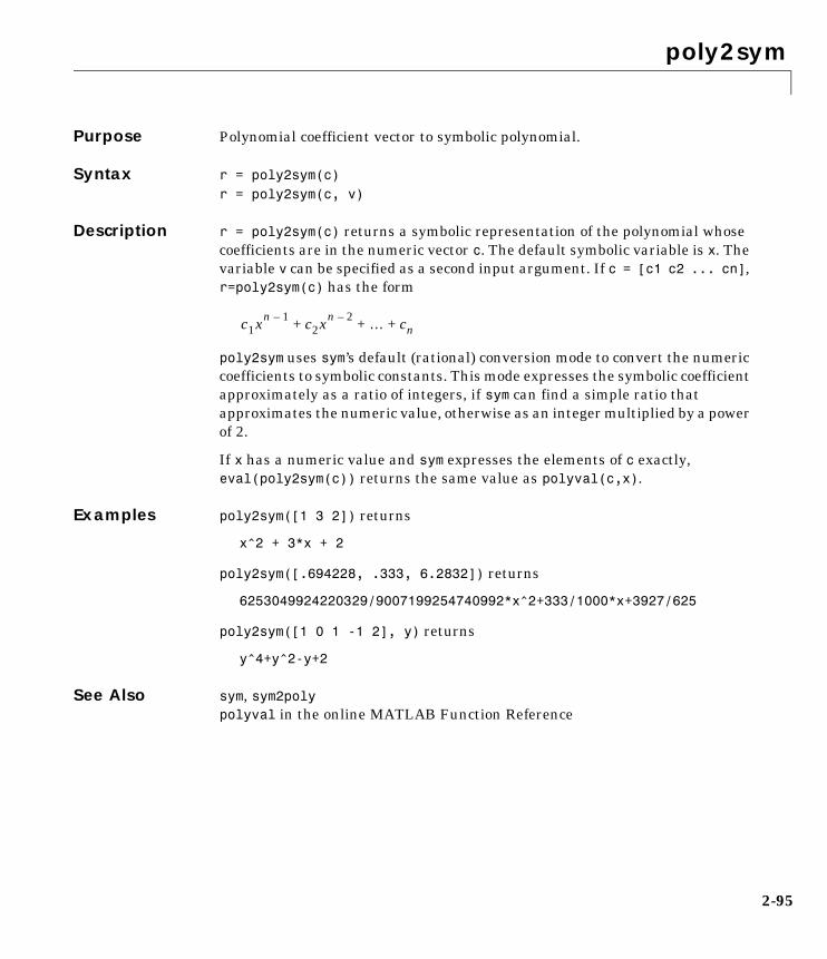
poly2sym
2-95
2poly2symPurpose Polynomial coefficient vector to symbolic polynomial.
Syntax r = poly2sym(c)r = poly2sym(c, v)
Description r = poly2sym(c) returns a symbolic representation of the polynomial whose coefficients are in the numeric vector c. The default symbolic variable is x. The variable v can be specified as a second input argument. If c = [c1 c2 ... cn], r=poly2sym(c) has the form
poly2sym uses sym’s default (rational) conversion mode to convert the numeric coefficients to symbolic constants. This mode expresses the symbolic coefficient approximately as a ratio of integers, if sym can find a simple ratio that approximates the numeric value, otherwise as an integer multiplied by a power of 2.
If x has a numeric value and sym expresses the elements of c exactly, eval(poly2sym(c)) returns the same value as polyval(c,x).
Examples poly2sym([1 3 2]) returns
x^2 + 3*x + 2
poly2sym([.694228, .333, 6.2832]) returns
6253049924220329/9007199254740992*x^2+333/1000*x+3927/625
poly2sym([1 0 1 -1 2], y) returns
y^4+y^2-y+2
See Also sym, sym2poly polyval in the online MATLAB Function Reference
c1xn 1– c2xn 2– … cn+ + +
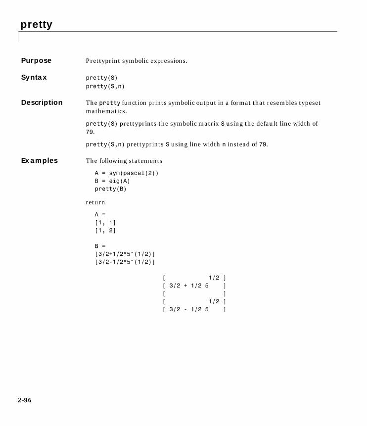
pretty
2-96
2prettyPurpose Prettyprint symbolic expressions.
Syntax pretty(S)pretty(S,n)
Description The pretty function prints symbolic output in a format that resembles typeset mathematics.
pretty(S) prettyprints the symbolic matrix S using the default line width of 79.
pretty(S,n) prettyprints S using line width n instead of 79.
Examples The following statements
A = sym(pascal(2))B = eig(A)pretty(B)
return
A =[1, 1][1, 2]
B =[3/2+1/2*5^(1/2)][3/2-1/2*5^(1/2)]
[ 1/2 ][ 3/2 + 1/2 5 ][ ][ 1/2 ][ 3/2 - 1/2 5 ]
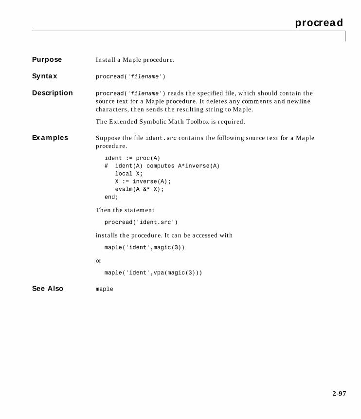
procread
2-97
2procreadPurpose Install a Maple procedure.
Syntax procread('filename')
Description procread('filename') reads the specified file, which should contain the source text for a Maple procedure. It deletes any comments and newline characters, then sends the resulting string to Maple.
The Extended Symbolic Math Toolbox is required.
Examples Suppose the file ident.src contains the following source text for a Maple procedure.
ident := proc(A)# ident(A) computes A*inverse(A)
local X;X := inverse(A);evalm(A &* X);
end;
Then the statement
procread('ident.src')
installs the procedure. It can be accessed with
maple('ident',magic(3))
or
maple('ident',vpa(magic(3)))
See Also maple

rank
2-98
2rankPurpose Symbolic matrix rank.
Syntax rank(A)
Description rank(A) is the rank of the symbolic matrix A.
Examples rank([a b;c d]) is 2.
rank(sym(magic(4))) is 3.

real
2-99
2realPurpose Symbolic real part.
Syntax real(Z)
Description real(Z) is the real part of a symbolic Z.
See Also conj, imag
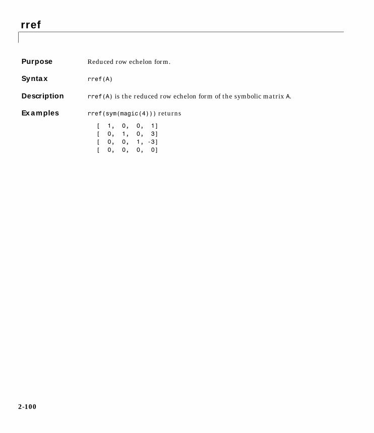
rref
2-100
2rrefPurpose Reduced row echelon form.
Syntax rref(A)
Description rref(A) is the reduced row echelon form of the symbolic matrix A.
Examples rref(sym(magic(4))) returns
[ 1, 0, 0, 1][ 0, 1, 0, 3][ 0, 0, 1, -3][ 0, 0, 0, 0]
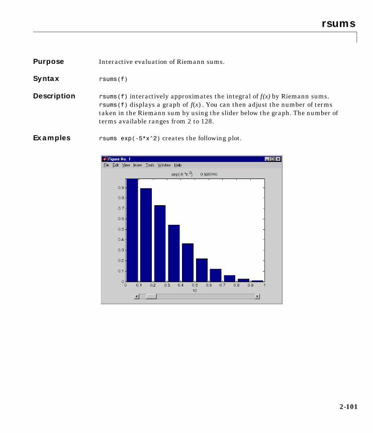
rsums
2-101
2rsumsPurpose Interactive evaluation of Riemann sums.
Syntax rsums(f)
Description rsums(f) interactively approximates the integral of f(x) by Riemann sums. rsums(f) displays a graph of . You can then adjust the number of terms taken in the Riemann sum by using the slider below the graph. The number of terms available ranges from 2 to 128.
Examples rsums exp(-5*x^2) creates the following plot.
f x( )
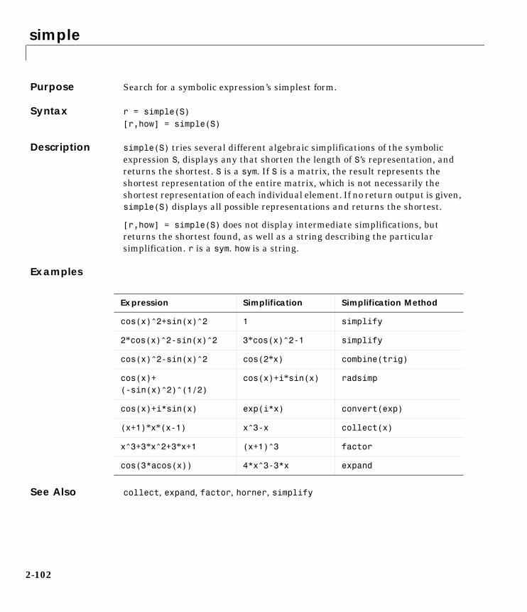
simple
2-102
2simplePurpose Search for a symbolic expression’s simplest form.
Syntax r = simple(S)[r,how] = simple(S)
Description simple(S) tries several different algebraic simplifications of the symbolic expression S, displays any that shorten the length of S’s representation, and returns the shortest. S is a sym. If S is a matrix, the result represents the shortest representation of the entire matrix, which is not necessarily the shortest representation of each individual element. If no return output is given, simple(S) displays all possible representations and returns the shortest.
[r,how] = simple(S) does not display intermediate simplifications, but returns the shortest found, as well as a string describing the particular simplification. r is a sym. how is a string.
Examples
See Also collect, expand, factor, horner, simplify
Expression Simplification Simplification Method
cos(x)^2+sin(x)^2 1 simplify
2*cos(x)^2-sin(x)^2 3*cos(x)^2-1 simplify
cos(x)^2-sin(x)^2 cos(2*x) combine(trig)
cos(x)+ (-sin(x)^2)^(1/2)
cos(x)+i*sin(x) radsimp
cos(x)+i*sin(x) exp(i*x) convert(exp)
(x+1)*x*(x-1) x^3-x collect(x)
x^3+3*x^2+3*x+1 (x+1)^3 factor
cos(3*acos(x)) 4*x^3-3*x expand
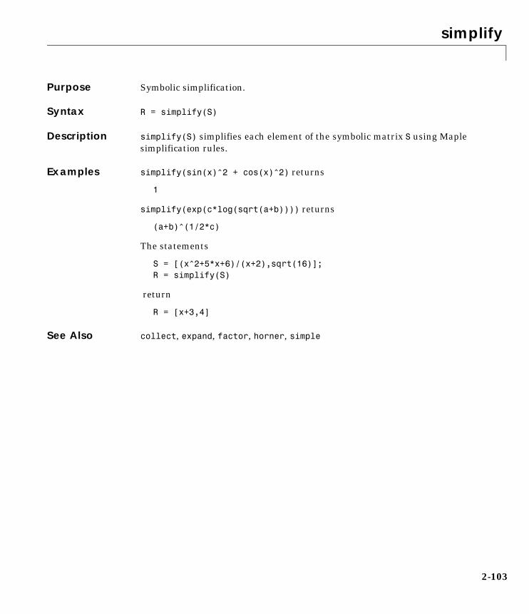
simplify
2-103
2simplifyPurpose Symbolic simplification.
Syntax R = simplify(S)
Description simplify(S) simplifies each element of the symbolic matrix S using Maple simplification rules.
Examples simplify(sin(x)^2 + cos(x)^2) returns
1
simplify(exp(c*log(sqrt(a+b)))) returns
(a+b)^(1/2*c)
The statements
S = [(x^2+5*x+6)/(x+2),sqrt(16)];R = simplify(S)
return
R = [x+3,4]
See Also collect, expand, factor, horner, simple
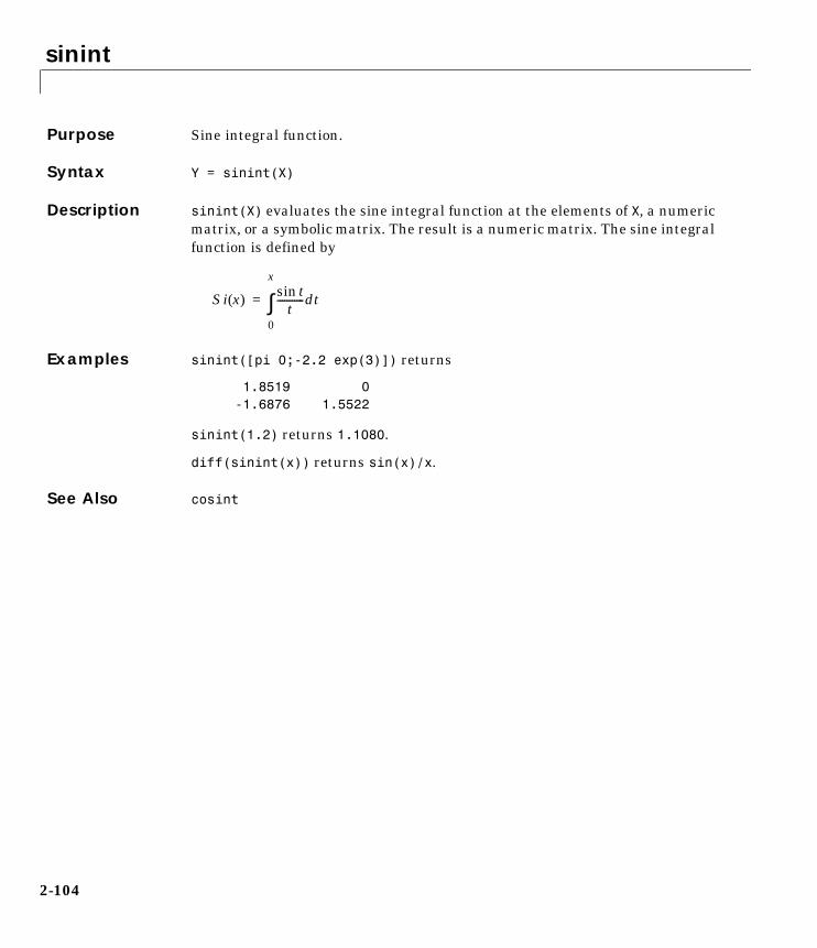
sinint
2-104
2sinintPurpose Sine integral function.
Syntax Y = sinint(X)
Description sinint(X) evaluates the sine integral function at the elements of X, a numeric matrix, or a symbolic matrix. The result is a numeric matrix. The sine integral function is defined by
Examples sinint([pi 0;-2.2 exp(3)]) returns
1.8519 0 -1.6876 1.5522
sinint(1.2) returns 1.1080.
diff(sinint(x)) returns sin(x)/x.
See Also cosint
Si x( )tsin
t----------- td
0
x
∫=
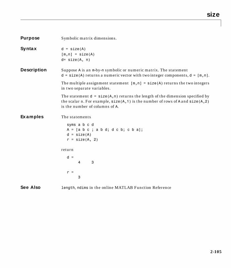
size
2-105
2sizePurpose Symbolic matrix dimensions.
Syntax d = size(A)[m,n] = size(A)d= size(A, n)
Description Suppose A is an m-by-n symbolic or numeric matrix. The statement d = size(A) returns a numeric vector with two integer components, d = [m,n].
The multiple assignment statement [m,n] = size(A) returns the two integers in two separate variables.
The statement d = size(A,n) returns the length of the dimension specified by the scalar n. For example, size(A,1) is the number of rows of A and size(A,2) is the number of columns of A.
Examples The statements
syms a b c dA = [a b c ; a b d; d c b; c b a];d = size(A)r = size(A, 2)
return
d = 4 3
r = 3
See Also length, ndims in the online MATLAB Function Reference
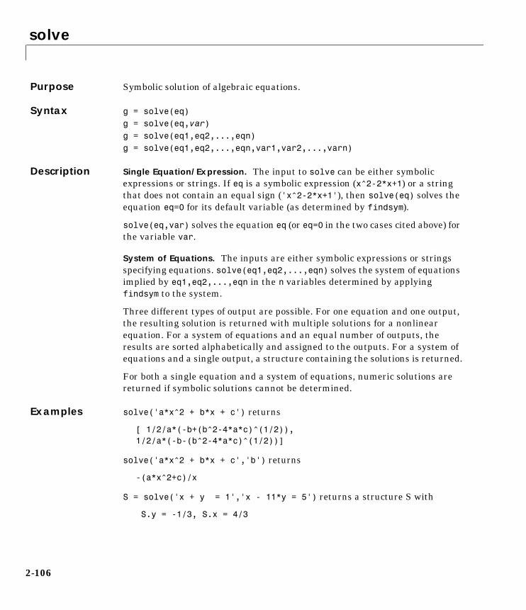
solve
2-106
2solvePurpose Symbolic solution of algebraic equations.
Syntax g = solve(eq)g = solve(eq,var)g = solve(eq1,eq2,...,eqn)g = solve(eq1,eq2,...,eqn,var1,var2,...,varn)
Description Single Equation/Expression. The input to solve can be either symbolic expressions or strings. If eq is a symbolic expression (x^2-2*x+1) or a string that does not contain an equal sign ('x^2-2*x+1'), then solve(eq) solves the equation eq=0 for its default variable (as determined by findsym).
solve(eq,var) solves the equation eq (or eq=0 in the two cases cited above) for the variable var.
System of Equations. The inputs are either symbolic expressions or strings specifying equations. solve(eq1,eq2,...,eqn) solves the system of equations implied by eq1,eq2,...,eqn in the n variables determined by applying findsym to the system.
Three different types of output are possible. For one equation and one output, the resulting solution is returned with multiple solutions for a nonlinear equation. For a system of equations and an equal number of outputs, the results are sorted alphabetically and assigned to the outputs. For a system of equations and a single output, a structure containing the solutions is returned.
For both a single equation and a system of equations, numeric solutions are returned if symbolic solutions cannot be determined.
Examples solve('a*x^2 + b*x + c') returns
[ 1/2/a*(-b+(b^2-4*a*c)^(1/2)), 1/2/a*(-b-(b^2-4*a*c)^(1/2))]
solve('a*x^2 + b*x + c','b') returns
-(a*x^2+c)/x
S = solve('x + y = 1','x - 11*y = 5') returns a structure S with
S.y = -1/3, S.x = 4/3

solve
2-107
A = solve('a*u^2 + v^2', 'u - v = 1', 'a^2 - 5*a + 6')
returns
A =
a: [4x1 sym] u: [4x1 sym] v: [4x1 sym]
where
A.a =[ 2][ 2][ 3][ 3]
A.u =[ 1/3+1/3*i*2^(1/2)][ 1/3-1/3*i*2^(1/2)][ 1/4+1/4*i*3^(1/2)][ 1/4-1/4*i*3^(1/2)]
A.v =[ -2/3+1/3*i*2^(1/2)][ -2/3-1/3*i*2^(1/2)][ -3/4+1/4*i*3^(1/2)][ -3/4-1/4*i*3^(1/2)]
See Also arithmetic operators, dsolve, findsym
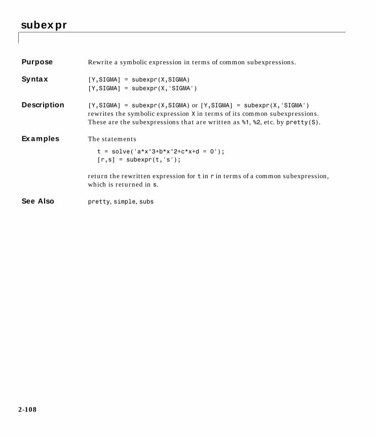
subexpr
2-108
2subexprPurpose Rewrite a symbolic expression in terms of common subexpressions.
Syntax [Y,SIGMA] = subexpr(X,SIGMA)[Y,SIGMA] = subexpr(X,'SIGMA')
Description [Y,SIGMA] = subexpr(X,SIGMA) or [Y,SIGMA] = subexpr(X,'SIGMA') rewrites the symbolic expression X in terms of its common subexpressions. These are the subexpressions that are written as %1, %2, etc. by pretty(S).
Examples The statements
t = solve('a*x^3+b*x^2+c*x+d = 0');[r,s] = subexpr(t,'s');
return the rewritten expression for t in r in terms of a common subexpression, which is returned in s.
See Also pretty, simple, subs
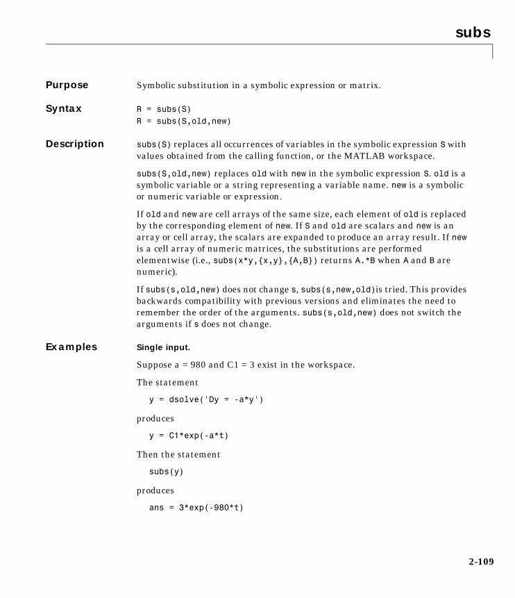
subs
2-109
2subsPurpose Symbolic substitution in a symbolic expression or matrix.
Syntax R = subs(S) R = subs(S,old,new)
Description subs(S) replaces all occurrences of variables in the symbolic expression S with values obtained from the calling function, or the MATLAB workspace.
subs(S,old,new) replaces old with new in the symbolic expression S. old is a symbolic variable or a string representing a variable name. new is a symbolic or numeric variable or expression.
If old and new are cell arrays of the same size, each element of old is replaced by the corresponding element of new. If S and old are scalars and new is an array or cell array, the scalars are expanded to produce an array result. If new is a cell array of numeric matrices, the substitutions are performed elementwise (i.e., subs(x*y,{x,y},{A,B}) returns A.*B when A and B are numeric).
If subs(s,old,new) does not change s, subs(s,new,old)is tried. This provides backwards compatibility with previous versions and eliminates the need to remember the order of the arguments. subs(s,old,new) does not switch the arguments if s does not change.
Examples Single input.
Suppose a = 980 and C1 = 3 exist in the workspace.
The statement
y = dsolve('Dy = -a*y')
produces
y = C1*exp(-a*t)
Then the statement
subs(y)
produces
ans = 3*exp(-980*t)
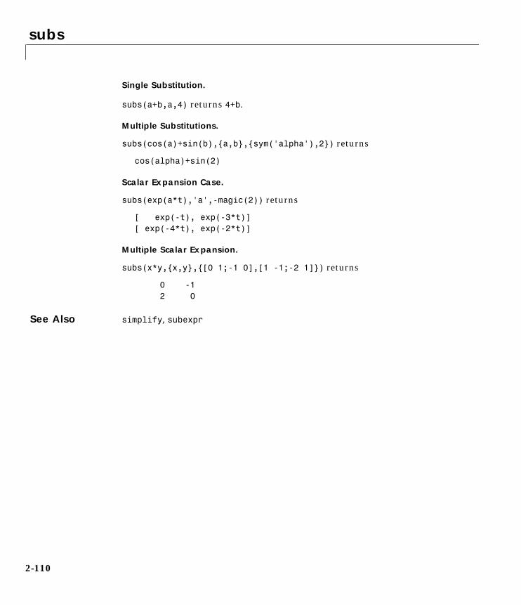
subs
2-110
Single Substitution.
subs(a+b,a,4) returns 4+b.
Multiple Substitutions.
subs(cos(a)+sin(b),{a,b},{sym('alpha'),2}) returns
cos(alpha)+sin(2)
Scalar Expansion Case.
subs(exp(a*t),'a',-magic(2)) returns
[ exp(-t), exp(-3*t)][ exp(-4*t), exp(-2*t)]
Multiple Scalar Expansion.
subs(x*y,{x,y},{[0 1;-1 0],[1 -1;-2 1]}) returns
0 -1 2 0
See Also simplify, subexpr
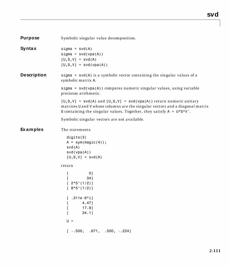
svd
2-111
2svdPurpose Symbolic singular value decomposition.
Syntax sigma = svd(A)sigma = svd(vpa(A))[U,S,V] = svd(A)[U,S,V] = svd(vpa(A))
Description sigma = svd(A) is a symbolic vector containing the singular values of a symbolic matrix A.
sigma = svd(vpa(A)) computes numeric singular values, using variable precision arithmetic.
[U,S,V] = svd(A) and [U,S,V] = svd(vpa(A)) return numeric unitary matrices U and V whose columns are the singular vectors and a diagonal matrix S containing the singular values. Together, they satisfy A = U*S*V'.
Symbolic singular vectors are not available.
Examples The statements
digits(3)A = sym(magic(4));svd(A)svd(vpa(A))[U,S,V] = svd(A)
return
[ 0][ 34][ 2*5^(1/2)][ 8*5^(1/2)]
[ .311e-6*i][ 4.47][ 17.9][ 34.1]
U = [ -.500, .671, .500, -.224]
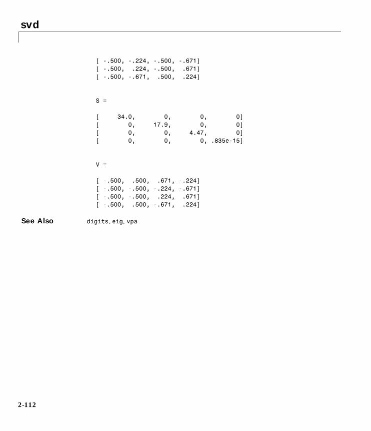
svd
2-112
[ -.500, -.224, -.500, -.671][ -.500, .224, -.500, .671][ -.500, -.671, .500, .224] S = [ 34.0, 0, 0, 0][ 0, 17.9, 0, 0][ 0, 0, 4.47, 0][ 0, 0, 0, .835e-15] V = [ -.500, .500, .671, -.224][ -.500, -.500, -.224, -.671][ -.500, -.500, .224, .671][ -.500, .500, -.671, .224]
See Also digits, eig, vpa
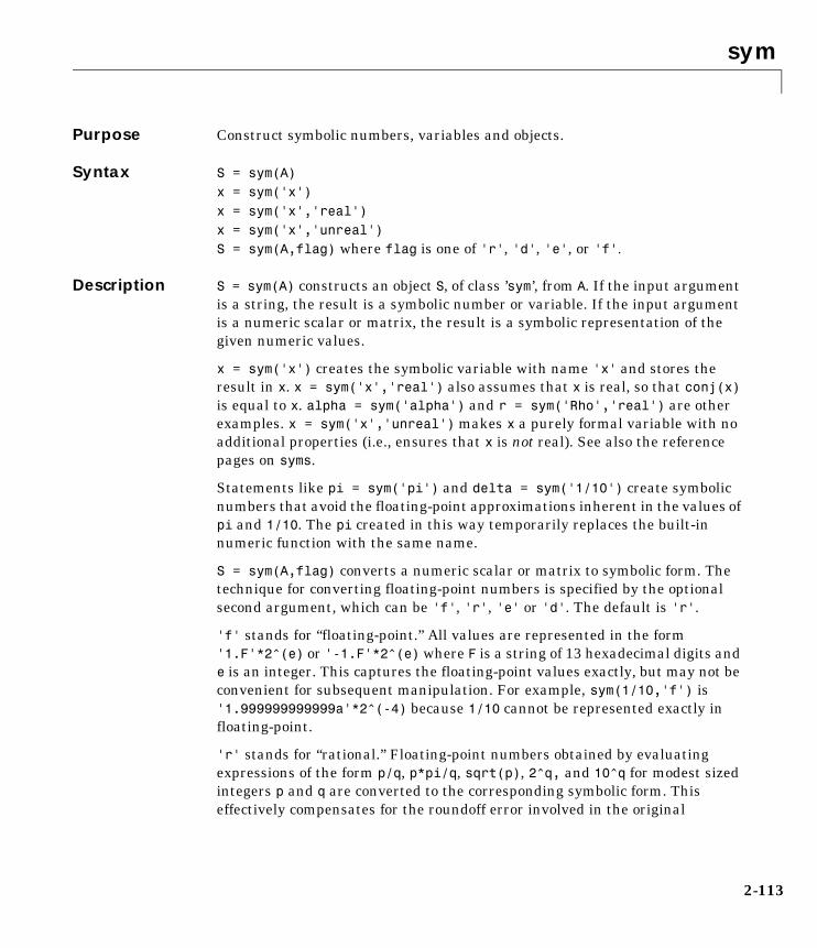
sym
2-113
2symPurpose Construct symbolic numbers, variables and objects.
Syntax S = sym(A)x = sym('x')x = sym('x','real')x = sym('x','unreal')S = sym(A,flag) where flag is one of 'r', 'd', 'e', or 'f'.
Description S = sym(A) constructs an object S, of class ’sym’, from A. If the input argument is a string, the result is a symbolic number or variable. If the input argument is a numeric scalar or matrix, the result is a symbolic representation of the given numeric values.
x = sym('x') creates the symbolic variable with name 'x' and stores the result in x. x = sym('x','real') also assumes that x is real, so that conj(x) is equal to x. alpha = sym('alpha') and r = sym('Rho','real') are other examples. x = sym('x','unreal') makes x a purely formal variable with no additional properties (i.e., ensures that x is not real). See also the reference pages on syms.
Statements like pi = sym('pi') and delta = sym('1/10') create symbolic numbers that avoid the floating-point approximations inherent in the values of pi and 1/10. The pi created in this way temporarily replaces the built-in numeric function with the same name.
S = sym(A,flag) converts a numeric scalar or matrix to symbolic form. The technique for converting floating-point numbers is specified by the optional second argument, which can be 'f', 'r', 'e' or 'd'. The default is 'r'.
'f' stands for “floating-point.” All values are represented in the form '1.F'*2^(e) or '-1.F'*2^(e) where F is a string of 13 hexadecimal digits and e is an integer. This captures the floating-point values exactly, but may not be convenient for subsequent manipulation. For example, sym(1/10,'f') is '1.999999999999a'*2^(-4) because 1/10 cannot be represented exactly in floating-point.
'r' stands for “rational.” Floating-point numbers obtained by evaluating expressions of the form p/q, p*pi/q, sqrt(p), 2^q, and 10^q for modest sized integers p and q are converted to the corresponding symbolic form. This effectively compensates for the roundoff error involved in the original
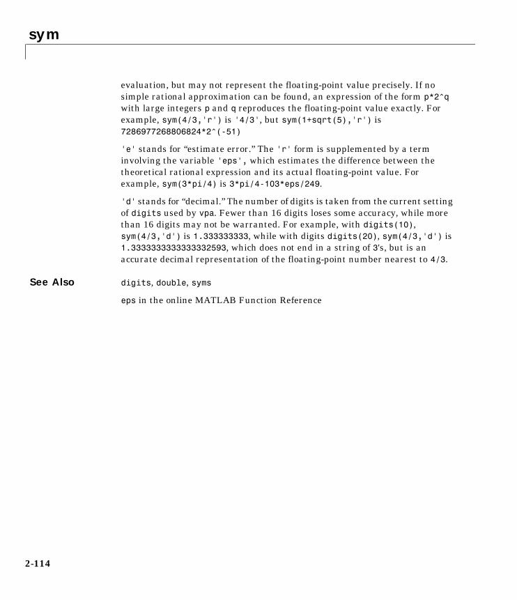
sym
2-114
evaluation, but may not represent the floating-point value precisely. If no simple rational approximation can be found, an expression of the form p*2^q with large integers p and q reproduces the floating-point value exactly. For example, sym(4/3,'r') is '4/3', but sym(1+sqrt(5),'r') is 7286977268806824*2^(-51)
'e' stands for “estimate error.” The 'r' form is supplemented by a term involving the variable 'eps', which estimates the difference between the theoretical rational expression and its actual floating-point value. For example, sym(3*pi/4) is 3*pi/4-103*eps/249.
'd' stands for “decimal.” The number of digits is taken from the current setting of digits used by vpa. Fewer than 16 digits loses some accuracy, while more than 16 digits may not be warranted. For example, with digits(10), sym(4/3,'d') is 1.333333333, while with digits digits(20), sym(4/3,'d') is 1.3333333333333332593, which does not end in a string of 3's, but is an accurate decimal representation of the floating-point number nearest to 4/3.
See Also digits, double, syms
eps in the online MATLAB Function Reference

syms
2-115
2symsPurpose Short-cut for constructing symbolic objects.
Syntax syms arg1 arg2 ...syms arg1 arg2 ... realsyms arg1 arg2 ... unreal
Description syms arg1 arg2 ... is short-hand notation for
arg1 = sym('arg1');arg2 = sym('arg2'); ...
syms arg1 arg2 ... real is short-hand notation for
arg1 = sym('arg1','real');arg2 = sym('arg2','real'); ...
syms arg1 arg2 ... unreal is short-hand notation for
arg1 = sym('arg1','unreal');arg2 = sym('arg2','unreal'); ...
Each input argument must begin with a letter and can contain only alphanumeric characters.
Examples syms x beta real is equivalent to
x = sym('x','real');beta = sym('beta','real');
To clear the symbolic objects x and beta of 'real' status, type
syms x beta unreal
Note clear x will not clear the symbolic object x of its status 'real'. You can achieve this, using the commands syms x unreal or clear mex or clear all. In the latter two cases, the Maple kernel will have to be reloaded in the MATLAB workspace. (This is inefficient and time consuming).
See Also sym
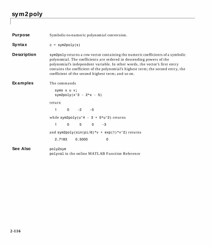
sym2poly
2-116
2sym2polyPurpose Symbolic-to-numeric polynomial conversion.
Syntax c = sym2poly(s)
Description sym2poly returns a row vector containing the numeric coefficients of a symbolic polynomial. The coefficients are ordered in descending powers of the polynomial’s independent variable. In other words, the vector’s first entry contains the coefficient of the polynomial’s highest term; the second entry, the coefficient of the second highest term; and so on.
Examples The commands
syms x u v;sym2poly(x^3 - 2*x - 5)
return
1 0 -2 -5
while sym2poly(u^4 - 3 + 5*u^2) returns
1 0 5 0 -3
and sym2poly(sin(pi/6)*v + exp(1)*v^2) returns
2.7183 0.5000 0
See Also poly2sym polyval in the online MATLAB Function Reference
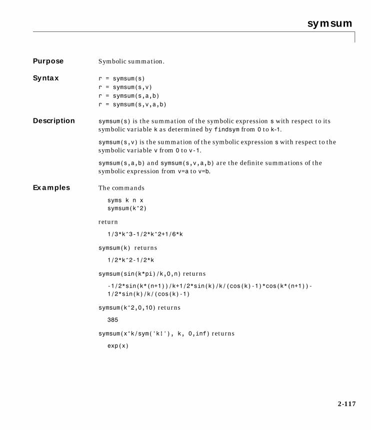
symsum
2-117
2symsumPurpose Symbolic summation.
Syntax r = symsum(s)r = symsum(s,v)r = symsum(s,a,b)r = symsum(s,v,a,b)
Description symsum(s) is the summation of the symbolic expression s with respect to its symbolic variable k as determined by findsym from 0 to k-1.
symsum(s,v) is the summation of the symbolic expression s with respect to the symbolic variable v from 0 to v-1.
symsum(s,a,b) and symsum(s,v,a,b) are the definite summations of the symbolic expression from v=a to v=b.
Examples The commands
syms k n xsymsum(k^2)
return
1/3*k^3-1/2*k^2+1/6*k
symsum(k) returns
1/2*k^2-1/2*k
symsum(sin(k*pi)/k,0,n) returns
-1/2*sin(k*(n+1))/k+1/2*sin(k)/k/(cos(k)-1)*cos(k*(n+1))-1/2*sin(k)/k/(cos(k)-1)
symsum(k^2,0,10) returns
385
symsum(x^k/sym('k!'), k, 0,inf) returns
exp(x)

symsum
2-118
Note The preceding example uses sym to create the symbolic expression k! in order to bypass MATLAB’s expression parser, which does not recognize ! as a factorial operator.
See Also findsym, int, syms
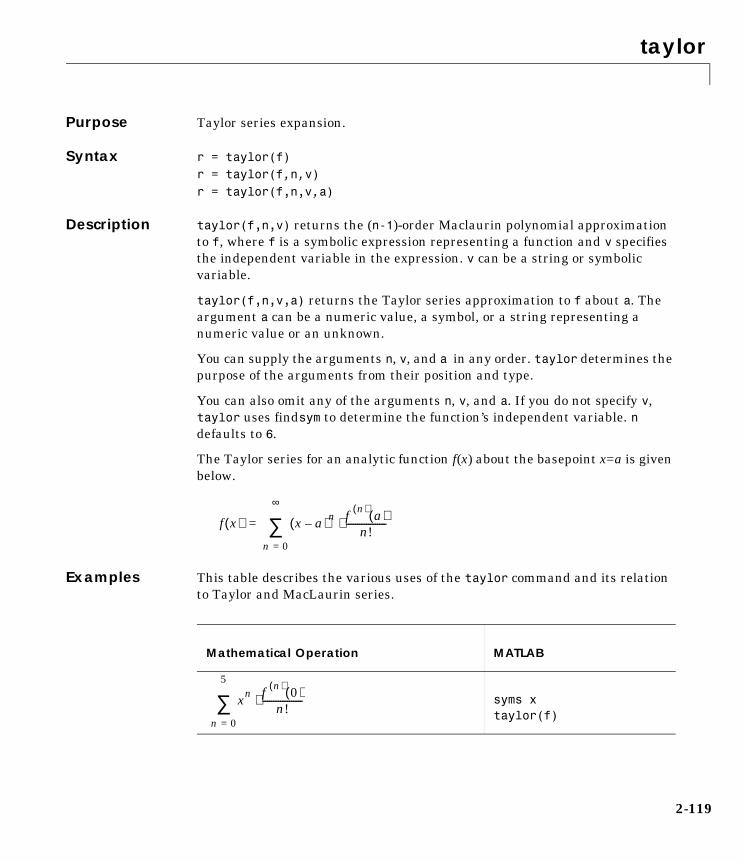
taylor
2-119
2taylorPurpose Taylor series expansion.
Syntax r = taylor(f)r = taylor(f,n,v)r = taylor(f,n,v,a)
Description taylor(f,n,v) returns the (n-1)-order Maclaurin polynomial approximation to f, where f is a symbolic expression representing a function and v specifies the independent variable in the expression. v can be a string or symbolic variable.
taylor(f,n,v,a) returns the Taylor series approximation to f about a. The argument a can be a numeric value, a symbol, or a string representing a numeric value or an unknown.
You can supply the arguments n, v, and a in any order. taylor determines the purpose of the arguments from their position and type.
You can also omit any of the arguments n, v, and a. If you do not specify v, taylor uses findsym to determine the function’s independent variable. n defaults to 6.
The Taylor series for an analytic function f(x) about the basepoint x=a is given below.
Examples This table describes the various uses of the taylor command and its relation to Taylor and MacLaurin series.
f x( ) x a–( )n f n( ) a( )n!
------------------⋅
n 0=
∞
∑=
Mathematical Operation MATLAB
syms xtaylor(f)
xn f n( ) 0( )n!
------------------⋅
n 0=
5
∑

taylor
2-120
In the case where f is a function of two or more variables (f=f(x,y,...)), there is a fourth parameter that allows you to select the variable for the Taylor expansion. Look at this table for illustrations of this feature.
, m is a positive integer taylor(f,m)m is a positive integer
, a is a real number taylor(f,a)a is a real number
m1, m2 are positive integers
taylor(f,m1,m2)m1, m2 are positive integers
a is real and m is a positive integer
taylor(f,m,a)a is real and m is a positive integer
Mathematical Operation MATLAB
taylor(f,y)
Mathematical Operation MATLAB
xn f n( ) 0( )n!
------------------⋅
n 0=
m
∑
x a–( )n f n( ) a( )n!
------------------⋅
n 0=
5
∑
x m2–( )n f n( ) m2( )n!
-----------------------⋅
n 0=
m1
∑
x a–( )n f n( ) a( )n!
------------------⋅
n 0=
m
∑
yn
n!------
yn
n
∂
∂ f x y 0=,( )⋅
n 0=
5
∑
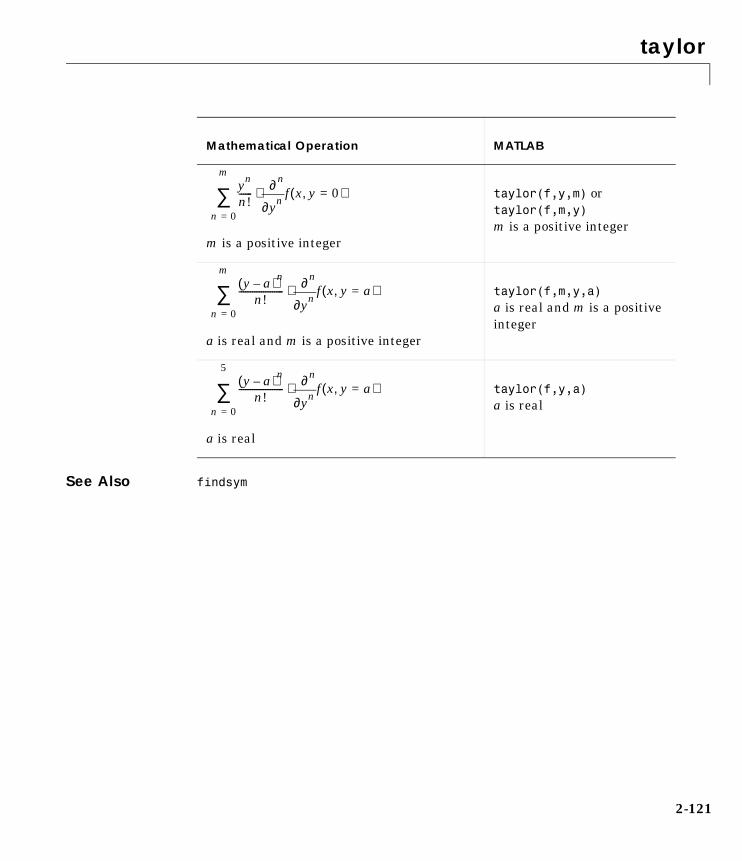
taylor
2-121
See Also findsym
m is a positive integer
taylor(f,y,m) or taylor(f,m,y)m is a positive integer
a is real and m is a positive integer
taylor(f,m,y,a)a is real and m is a positive integer
a is real
taylor(f,y,a)a is real
Mathematical Operation MATLAB
yn
n!------
yn
n
∂
∂ f x y 0=,( )⋅
n 0=
m
∑
y a–( )n
n!--------------------
yn
n
∂
∂ f x y a=,( )⋅
n 0=
m
∑
y a–( )n
n!--------------------
yn
n
∂
∂ f x y a=,( )⋅
n 0=
5
∑
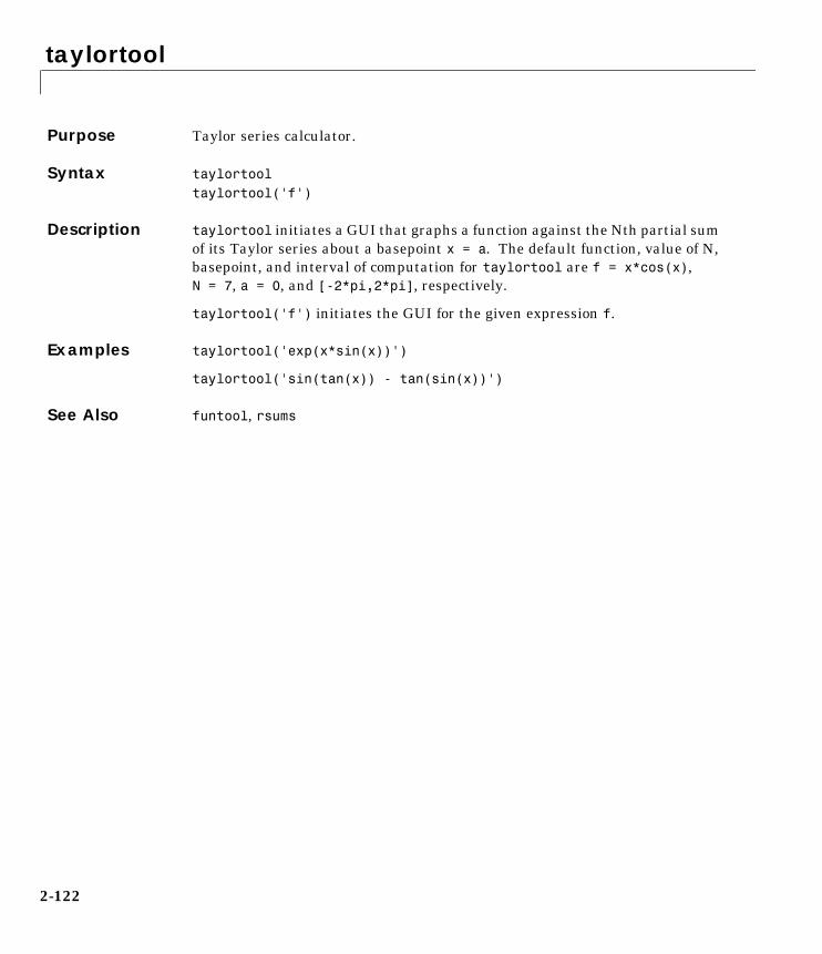
taylortool
2-122
2taylortoolPurpose Taylor series calculator.
Syntax taylortooltaylortool('f')
Description taylortool initiates a GUI that graphs a function against the Nth partial sum of its Taylor series about a basepoint x = a. The default function, value of N, basepoint, and interval of computation for taylortool are f = x*cos(x),N = 7, a = 0, and [-2*pi,2*pi], respectively.
taylortool('f') initiates the GUI for the given expression f.
Examples taylortool('exp(x*sin(x))')
taylortool('sin(tan(x)) - tan(sin(x))')
See Also funtool, rsums
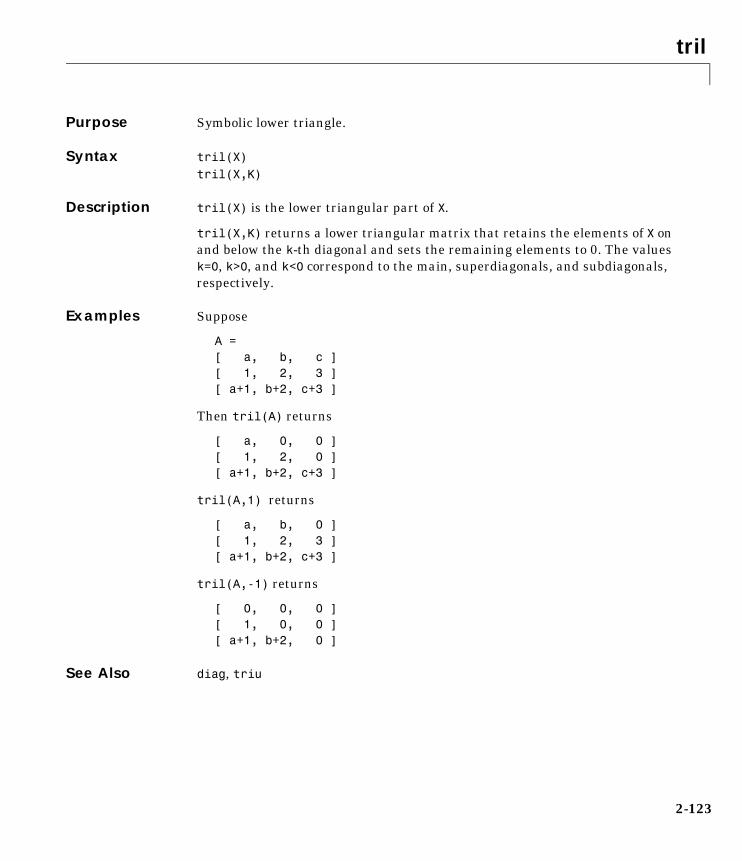
tril
2-123
2trilPurpose Symbolic lower triangle.
Syntax tril(X)tril(X,K)
Description tril(X) is the lower triangular part of X.
tril(X,K) returns a lower triangular matrix that retains the elements of X on and below the k-th diagonal and sets the remaining elements to 0. The values k=0, k>0, and k<0 correspond to the main, superdiagonals, and subdiagonals, respectively.
Examples Suppose
A =[ a, b, c ][ 1, 2, 3 ][ a+1, b+2, c+3 ]
Then tril(A) returns
[ a, 0, 0 ][ 1, 2, 0 ][ a+1, b+2, c+3 ]
tril(A,1) returns
[ a, b, 0 ][ 1, 2, 3 ][ a+1, b+2, c+3 ]
tril(A,-1) returns
[ 0, 0, 0 ][ 1, 0, 0 ][ a+1, b+2, 0 ]
See Also diag, triu
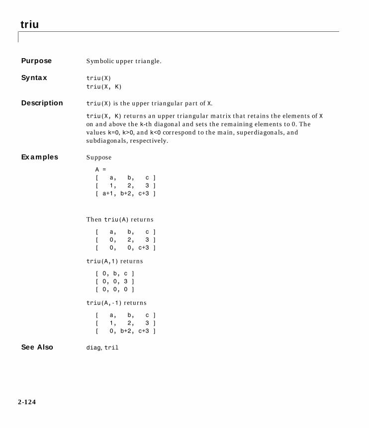
triu
2-124
2triuPurpose Symbolic upper triangle.
Syntax triu(X)triu(X, K)
Description triu(X) is the upper triangular part of X.
triu(X, K) returns an upper triangular matrix that retains the elements of X on and above the k-th diagonal and sets the remaining elements to 0. The values k=0, k>0, and k<0 correspond to the main, superdiagonals, and subdiagonals, respectively.
Examples Suppose
A =[ a, b, c ][ 1, 2, 3 ][ a+1, b+2, c+3 ]
Then triu(A) returns
[ a, b, c ][ 0, 2, 3 ][ 0, 0, c+3 ]
triu(A,1) returns
[ 0, b, c ][ 0, 0, 3 ][ 0, 0, 0 ]
triu(A,-1) returns
[ a, b, c ][ 1, 2, 3 ][ 0, b+2, c+3 ]
See Also diag, tril
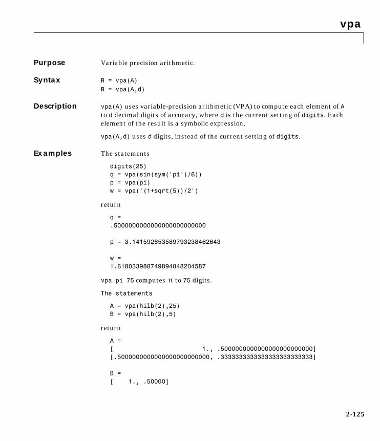
vpa
2-125
2vpaPurpose Variable precision arithmetic.
Syntax R = vpa(A)R = vpa(A,d)
Description vpa(A) uses variable-precision arithmetic (VPA) to compute each element of A to d decimal digits of accuracy, where d is the current setting of digits. Each element of the result is a symbolic expression.
vpa(A,d) uses d digits, instead of the current setting of digits.
Examples The statements
digits(25)q = vpa(sin(sym('pi')/6))p = vpa(pi)w = vpa('(1+sqrt(5))/2')
return
q =.5000000000000000000000000
p = 3.141592653589793238462643
w =1.618033988749894848204587
vpa pi 75 computes to 75 digits.
The statements
A = vpa(hilb(2),25)B = vpa(hilb(2),5)
return
A =[ 1., .5000000000000000000000000][.5000000000000000000000000, .3333333333333333333333333]
B =[ 1., .50000]
π
vpa
2-126
[.50000, .33333]
See Also digits, double
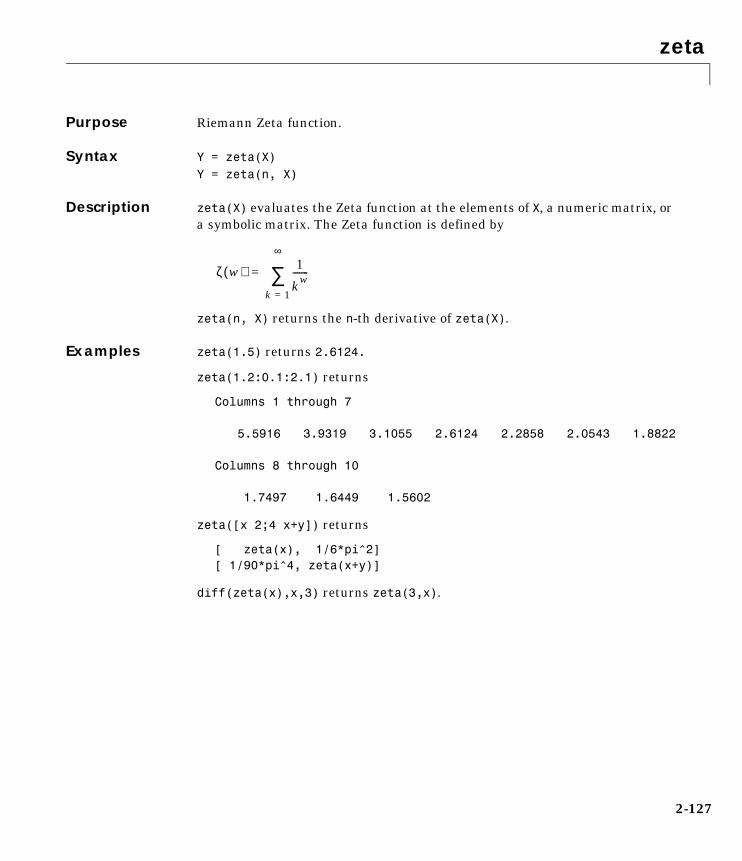
zeta
2-127
2zetaPurpose Riemann Zeta function.
Syntax Y = zeta(X)Y = zeta(n, X)
Description zeta(X) evaluates the Zeta function at the elements of X, a numeric matrix, or a symbolic matrix. The Zeta function is defined by
zeta(n, X) returns the n-th derivative of zeta(X).
Examples zeta(1.5) returns 2.6124.
zeta(1.2:0.1:2.1) returns
Columns 1 through 7 5.5916 3.9319 3.1055 2.6124 2.2858 2.0543 1.8822 Columns 8 through 10 1.7497 1.6449 1.5602
zeta([x 2;4 x+y]) returns
[ zeta(x), 1/6*pi^2][ 1/90*pi^4, zeta(x+y)]
diff(zeta(x),x,3) returns zeta(3,x).
ζ w( ) 1
kw-------
k 1=
∞
∑=
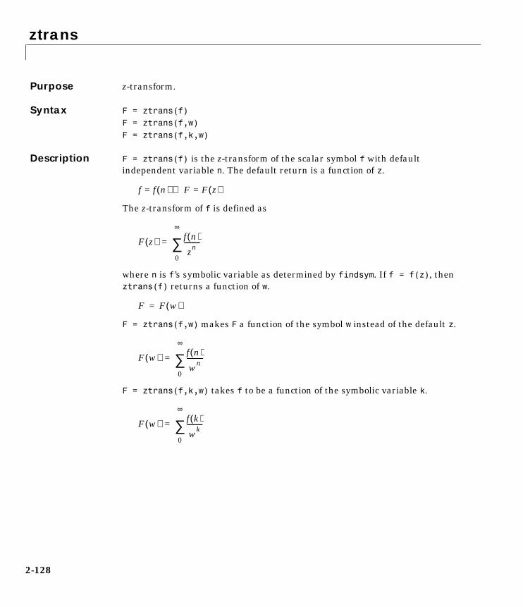
ztrans
2-128
2ztransPurpose z-transform.
Syntax F = ztrans(f)F = ztrans(f,w)F = ztrans(f,k,w)
Description F = ztrans(f) is the z-transform of the scalar symbol f with default independent variable n. The default return is a function of z.
The z-transform of f is defined as
where n is f’s symbolic variable as determined by findsym. If f = f(z), then ztrans(f) returns a function of w.
F = ztrans(f,w) makes F a function of the symbol w instead of the default z.
F = ztrans(f,k,w) takes f to be a function of the symbolic variable k.
f f n( )= F F z( )=⇒
F z( ) f n( )
zn----------
0
∞
∑=
F F w( )=
F w( ) f n( )
wn----------
0
∞
∑=
F w( ) f k( )
wk----------
0
∞
∑=
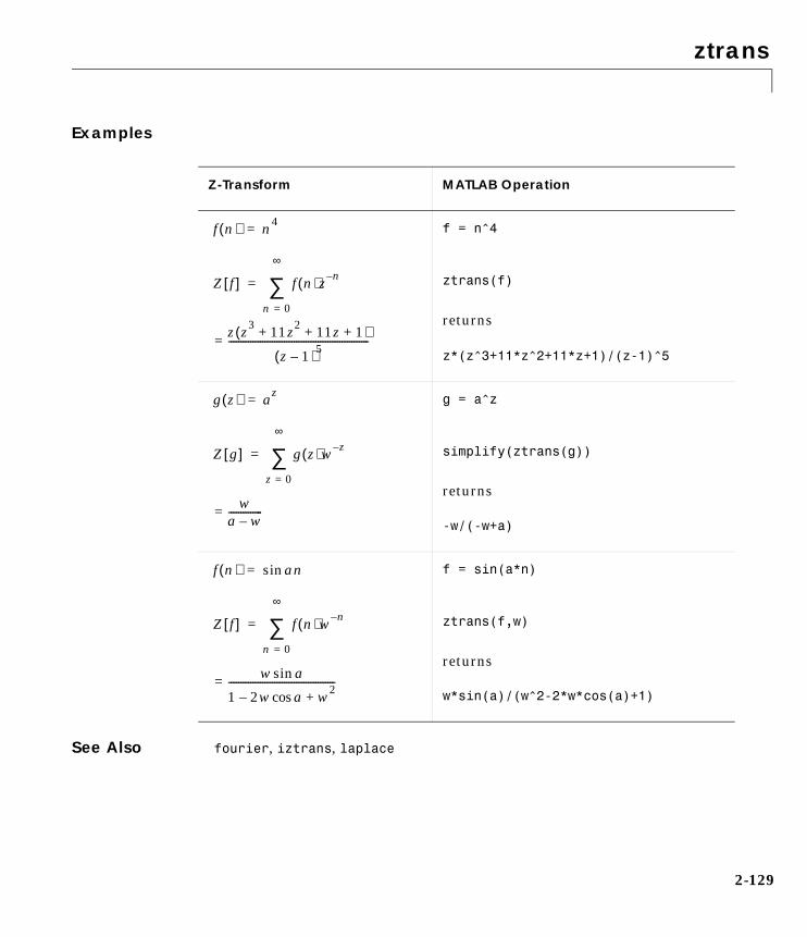
ztrans
2-129
Examples
See Also fourier, iztrans, laplace
Z-Transform MATLAB Operation
f = n^4
ztrans(f)
returns
z*(z^3+11*z^2+11*z+1)/(z-1)^5
g = a^z
simplify(ztrans(g))
returns
-w/(-w+a)
f = sin(a*n)
ztrans(f,w)
returns
w*sin(a)/(w^2-2*w*cos(a)+1)
f n( ) n4=
Z f[ ] f n( )z n–
z z3 11z2 11z 1+ + +( )
z 1–( )5----------------------------------------------------------=
n 0=
∞
∑=
g z( ) az=
Z g[ ] g z( )w z–
wa w–--------------=
z 0=
∞
∑=
f n( ) ansin=
Z f[ ] f n( )w n–
w asin
1 2w acos– w2+
--------------------------------------------=
n 0=
∞
∑=

ztrans
2-130
A
Compatibility Guide
Compatibility with Earlier Versions . . . . . . . . . A-2
Obsolete Functions . . . . . . . . . . . . . . . . . A-3
A Compatibility Guide
A-2
Compatibility with Earlier VersionsEarlier versions of the Symbolic Math Toolboxes work with version 4.0 or 4.1 of MATLAB and version V, release 2 of Maple. The goal was to provide access to Maple with a language syntax that is familiar to MATLAB users. This was been done without modifying either of the two underlying systems.
However, it is not possible to provide completely seamless integration without modifying MATLAB. For example, if f and g are strings representing symbolic expressions, we would prefer to use the notation f+g for their sum, instead of symadd(f,g). But f+g attempts to add the individual characters in the two strings, rather than concatenate them with a plus sign in between. Similarly, if A is a matrix whose elements are symbolic expressions, we would prefer to use A(i,j) to access a individual expression, instead of sym(A,i,j). But if A is a matrix of strings, then A(i,j) is a single character, not a complete expression.
This version of the Symbolic Math Toolboxes makes extensive use of the new MATLAB object capabilities and works with Maple V, Release 5. For this reason, it is not fully compatible with version 1 of the Symbolic Math Toolbox.

Obsolete Functions
A-3
Obsolete FunctionsThis version maintains some compatibility with version 1. For example, the following obsolete functions continue to be available in version 2, though you should avoid using them as future releases may not include them.
In version 1, these functions accepted strings as arguments and returned strings as results. In version 2, they accept either strings or symbolic objects as input arguments and produce symbolic objects as results. Version 2 provides overloaded MATLAB operators or new functions that you can use to replace most of these functions in your existing code.
For example, the version 1 statements
f = '1/(5+4*cos(x))'g = int(int(diff(f,2)))e = symsub(f,g)simple(e)
Function Description
determ Symbolic matrix determinant
linsolve Solve simultaneous linear equations
eigensys Symbolic eigenvalues and eigenvectors
singvals Symbolic singular values and singular vectors
numeric Convert symbolic matrix to numeric form
symop Symbolic operations
symadd Add symbolic expressions
symsub Subtract symbolic expressions
symmul Multiply symbolic expressions
symdiv Divide symbolic expressions
sympow Power of symbolic expression
eval Evaluate a symbolic expression
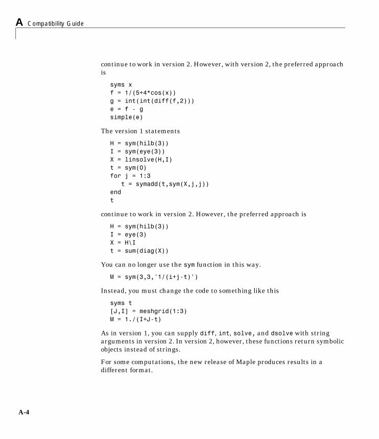
A Compatibility Guide
A-4
continue to work in version 2. However, with version 2, the preferred approach is
syms xf = 1/(5+4*cos(x))g = int(int(diff(f,2)))e = f - gsimple(e)
The version 1 statements
H = sym(hilb(3))I = sym(eye(3))X = linsolve(H,I)t = sym(0)for j = 1:3 t = symadd(t,sym(X,j,j))endt
continue to work in version 2. However, the preferred approach is
H = sym(hilb(3))I = eye(3)X = H\It = sum(diag(X))
You can no longer use the sym function in this way.
M = sym(3,3,'1/(i+j-t)')
Instead, you must change the code to something like this
syms t[J,I] = meshgrid(1:3)M = 1./(I+J-t)
As in version 1, you can supply diff, int, solve, and dsolve with string arguments in version 2. In version 2, however, these functions return symbolic objects instead of strings.
For some computations, the new release of Maple produces results in a different format.
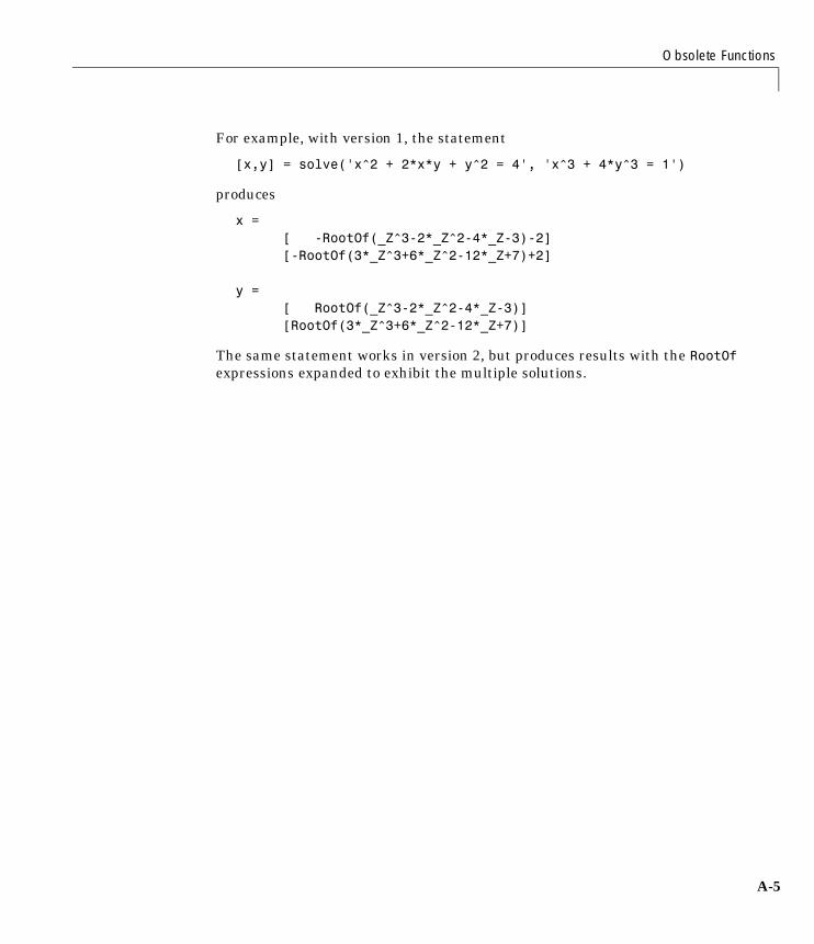
Obsolete Functions
A-5
For example, with version 1, the statement
[x,y] = solve('x^2 + 2*x*y + y^2 = 4', 'x^3 + 4*y^3 = 1')
produces
x = [ -RootOf(_Z^3-2*_Z^2-4*_Z-3)-2] [-RootOf(3*_Z^3+6*_Z^2-12*_Z+7)+2] y = [ RootOf(_Z^3-2*_Z^2-4*_Z-3)] [RootOf(3*_Z^3+6*_Z^2-12*_Z+7)]
The same statement works in version 2, but produces results with the RootOf expressions expanded to exhibit the multiple solutions.

A Compatibility Guide
A-6
I-1
Index
Symbols- 2-8* 2-8+ 2-8. 2-8.* 2-8./ 2-8.^ 2-9.’ 2-9/ 2-8@sym directory 1-16\ 1-67, 2-8^ 2-9’ 2-9
Aabstract functions 1-11Airy differential equation 1-96Airy function 1-96, 1-97algebraic equations
solving 2-106all 2-29arithmetic operations 2-8
left divisionarray 2-8matrix 2-8
matrix addition 2-8matrix subtraction 2-8multiplication
array 2-8matrix 2-8
powerarray 2-9matrix 2-9
right divisionarray 2-8
matrix 2-8transpose
array 2-9matrix 2-9
Bbackslash operator 1-67Bernoulli polynomials 1-97Bessel functions 1-98
differentiating 1-18integrating 1-25
besselj 1-18besselk 1-96beta function 1-98binomial coefficients 1-97branch cut 1-43
Ccalculus 1-17ccode 2-11characteristic polynomial 1-71, 1-73, 2-94Chebyshev polynomial 1-99circulant matrix 1-12, 1-55clear 1-27clearing variables
Maple workspace 1-27MATLAB workspace 1-27, 2-115
collect 1-45, 2-12colspace 2-13column space 1-68complementary error function 1-98complex conjugate 2-15complex number
imaginary part of 2-64
Index
I-2
real part of 2-99complex symbolic variables 1-10compose 2-14conj 1-10, 2-15converting symbolic matrices to numeric form
1-9cosine integral function 2-16cosine integrals 1-98cosint 2-16
DDawson’s integral 1-98decimal symbolic expressions 1-9definite integration 1-24det 2-17diag 2-18diff 1-17, 2-20differentiation 1-17diffraction 1-99digamma function 1-98digits 1-9, 2-21Dirac Delta function 1-98discontinuities 1-42discrim 1-86double 2-22
converting to floating-point with 1-63dsolve 1-93, 2-23
Eeig 1-70, 2-25eigenvalue trajectories 1-80eigenvalues 1-70, 1-81, 2-25
computing 1-70eigenvector 1-71elliptic integrals 1-98
eps 1-9error function 1-98Euler polynomials 1-97expand 1-46, 2-28expm 2-27exponential integrals 1-98Extended Symbolic Math Toolbox 1-2, 1-109, 2-89
orthogonal polynomials included with 1-98ezplot 1-31
Ffactor 2-47
example 1-47factorial function 1-11factorial operator 2-118findsym 1-14, 2-48finverse 2-49floating-pint arithmetic
IEEE 1-61floating-point arithmetic 1-60floating-point symbolic expressions 1-8format 1-60fortran 2-50fourier 2-51Fourier transform 2-51Fresnel integral 1-98function calculator 2-54functional composition 2-14functional inverse 2-49funtool 2-54
Ggamma function 1-98Gegenbauer polynomial 1-98generalized hypergeometric function 1-98
Index
I-3
Givens transformation 1-65, 1-74golden ratio 1-7
Hharmonic function 1-98Heaviside function 1-98Hermite polynomial 1-98Hilbert matrix 1-9, 1-66horner 2-57
example 1-46hyperbolic cosine function 1-98hyperbolic sine function 1-98hypergeometric function 1-98
IIEEE floating-point arithmetic 1-61ifourier 2-59ilaplace 2-62imag 2-64incomplete gamma function 1-98initializing the Maple kernel 2-80initstring variable 2-80int 1-23, 2-65
example 1-23integration 1-23
definite 1-24with real constants 1-25
inv 2-66inverse Fourier transform 2-59inverse Laplace transform 2-62inverse z-transform 2-68iztrans 2-68
JJacobi polynomial 1-99jacobian 1-19, 2-70Jacobian matrix 1-19, 2-70jordan 2-71
example 1-76Jordan canonical form 1-76, 2-71
LLaguerre polynomial 1-98Lambert’s W function 1-98, 2-73lambertw 2-73laplace 2-74Laplace transform 2-74latex 2-76left division
array 2-8matrix 2-8
Legendre polynomial 1-99limit 1-21, 2-77limits 1-20
two-sided 1-21undefined 1-21
linear algebra 1-65logarithm function 1-98logarithmic integral 1-98
Mmachine epsilon 1-9Maclaurin series 1-29Maple 1-2maple 2-78
output argument 1-107Maple functions
accessing 1-11, 1-102
Index
I-4
Maple help 2-91Maple kernel
accessing 2-78initializing 2-80
Maple library 2-80Maple Orthogonal Polynomial Package 2-89Maple packages 1-109
loading 1-110Maple procedure 1-109, 2-97
compiling 1-114installing 2-97writing 1-111
mapleinit 2-80matrix
addition 2-8condition number 1-68diagonal 2-18exponential 2-27inverse 2-66left division 2-8lower triangular 2-123multiplication 2-8power 2-9rank 2-98right division 2-8size 2-105subtraction 2-8transpose 2-9upper triangular 2-124
M-filecreating 1-16
mfun 1-97, 2-81mfunlist 2-82mhelp 2-91multiplication
array 2-8matrix 2-8
Nnull 2-92null space 1-68null space basis 2-92numden 2-93numeric symbolic expressions 1-8
Oordinary differential equations
solving 2-23orthogonal polynomials 1-98, 2-89
Ppoly 1-71, 2-94poly2sym 2-95polygamma function 1-98polynomial discriminants 1-86power
array 2-9matrix 2-9
pretty 2-96example 1-29
procread 1-112, 2-97prod 1-12
Rrank 2-98rational arithmetic 1-61rational symbolic expressions 1-8real 2-99real property 1-10real symbolic variables 1-10, 1-27reduced row echelon form 2-100Riemann sums
Index
I-5
evaluating 2-101Riemann Zeta function 1-97, 2-127right division
array 2-8matrix 2-8
Rosser matrix 1-72rref 2-100rsums 2-101
Sshifted sine integral 1-98simple 1-49, 2-102simplifications 1-44simplify 1-49, 2-103simultaneous differential equations
solving 1-95simultaneous linear equations
solving systems of 1-67, 1-92sine integral function 2-104sine integrals 1-98singular value decomposition 1-77, 2-111sinint 2-104solve 1-89, 2-106solving equations 1-89
algebraic 1-89, 2-106ordinary differential 1-93, 2-23
special functions 1-97evaluating numerically 2-81listing 2-82
spherical coordinates 1-19subexpr 1-53, 2-108subexpressions 1-53subs 1-55, 2-109substitutions 1-53
in symbolic expressions 2-109summation
symbolic 1-28svd 1-78, 2-111sym 1-6, 1-7, 1-8, 1-9, 1-11, 1-27, 2-113sym2poly 2-116symbolic expressions 1-89
C code representation of 2-11creating 1-7decimal 1-9differentiating 2-20expanding 2-28factoring 2-47finding variables in 2-48floating-point 1-8Fortran representation of 2-50integrating 2-65LaTeX representation of 2-76limit of 2-77numeric 1-8prettyprinting 2-96rational 1-8simplifying 2-102, 2-103, 2-108substituting in 2-109summation of 2-117Taylor series expansion of 2-119
symbolic math functionscreating 1-15
symbolic math programsdebugging 1-106writing 1-102
Symbolic Math Toolboxcompatibility with earlier versions A-2demo 1-6obsolete functions A-3
symbolic matrixcomputing eigenvalue of 1-73converting to numeric form 1-9creating 1-12
Index
I-6
differentiating 1-18symbolic objects
about 1-6creating 2-113, 2-115
symbolic polynomialsconverting to numeric form 2-116creating from coefficient vector 2-95Horner representation of 2-57
symbolic summation 1-28symbolic variables
clearing 2-115complex 1-10creating 1-7default 1-13real 1-10, 1-27
syms 1-8, 2-115symsize 2-105symsum 1-28, 2-117
Ttaylor 1-29, 2-119Taylor series 1-29Taylor series expansion 2-119taylortool 2-122trace mode 1-107transpose
array 2-9matrix 2-9
tril 2-123triu 2-124
Uunreal property 1-10
Vvariable-precision arithmetic 1-60, 2-125
setting accuracy of 2-21variable-precision numbers 1-62vpa 1-62, 2-125
Zzeta 2-127ztrans 2-128z-transform 2-128