structure and dynamics of the martian lower and middle

Structure and dynamics of the Martian lower and middleatmosphere as observed by the Mars Climate Sounder:Seasonal variations in zonal mean temperature, dust,and water ice aerosols

D. J. McCleese,1 N. G. Heavens,2 J. T. Schofield,1 W. A. Abdou,1 J. L. Bandfield,3

S. B. Calcutt,4 P. G. J. Irwin,4 D. M. Kass,1 A. Kleinböhl,1 S. R. Lewis,5 D. A. Paige,6

P. L. Read,4 M. I. Richardson,7 J. H. Shirley,1 F. W. Taylor,4 N. Teanby,4

and R. W. Zurek1

Received 14 June 2010; revised 3 September 2010; accepted 28 September 2010; published 28 December 2010.

[1] The first Martian year and a half of observations by the Mars Climate Sounder aboardthe Mars Reconnaissance Orbiter has revealed new details of the thermal structure anddistributions of dust and water ice in the atmosphere. The Martian atmosphere is shown inthe observations by the Mars Climate Sounder to vary seasonally between two modes:a symmetrical equinoctial structure with middle atmosphere polar warming and a solstitialstructure with an intense middle atmosphere polar warming overlying a deep winter polarvortex. The dust distribution, in particular, is more complex than appreciated before theadvent of these high (∼5 km) vertical resolution observations, which extend from near thesurface to above 80 km and yield 13 dayside and 13 nightside pole‐to‐pole cross sectionseach day. Among the new features noted is a persistent maximum in dust mass mixing ratioat 15–25 km above the surface (at least on the nightside) during northern spring andsummer. The water ice distribution is very sensitive to the diurnal and seasonal variationof temperature and is a good tracer of the vertically propagating tide.

Citation: McCleese, D. J., et al. (2010), Structure and dynamics of the Martian lower and middle atmosphere as observed by theMars Climate Sounder: Seasonal variations in zonal mean temperature, dust, and water ice aerosols, J. Geophys. Res., 115,E12016, doi:10.1029/2010JE003677.

1. Introduction

[2] The Mars Climate Sounder (MCS) [McCleese et al.,2007] on Mars Reconnaissance Orbiter (MRO) [Zurek andSmrekar, 2007] has been observing the Martian atmo-sphere since September of 2006. MCS observes the limb ofthe atmosphere in one broadband visible and eight infraredchannels in the 0.3 to 50 mm spectral range. MCS data canbe used to determine the thermal structure of the atmospherefrom the surface to 80 km at a vertical resolution of ∼5 km(approximately one half the atmospheric scale height). Thus,

MCS bridges the gap between observations of the loweratmosphere provided by nadir infrared spectroscopy [Smithet al., 2001; Smith, 2004], from which an extensive clima-tology has been developed, and radio occultation [Hinson etal., 2004], and measurements in the upper atmosphere ob-tained from aerobraking experiments [Keating et al., 1998],and stellar occultation [Forget et al., 2009]. MCS data isalso used to simultaneously profile the aerosol structure ofthe atmosphere with the same vertical range and resolutionas its temperature observations.[3] Initial retrievals from MCS data have been used to

investigate the temperature maximum in the polar middleatmosphere during southern hemisphere winter [McCleeseet al., 2008] and the atmospheric thermal tides [Lee et al.,2009]. Today, there are over 106 MCS profiles of temper-ature, dust, and water ice [Kleinböhl et al., 2009] spanningthe full seasonal cycle with some seasons sampled overmultiple years.[4] In this paper, we describe the seasonal cycle of the

zonal average thermal structure and aerosol distributionsduring the first 1.5 Mars years of observations by MCS. Wefocus on Mars Year (MY) 29 (see Clancy et al. [2000] for adescription of the convention), for which we have nearlycomplete observational coverage and during which there

1Jet Propulsion Laboratory, California Institute of Technology,Pasadena, California, USA.

2Division of Geological and Planetary Sciences, California Institute ofTechnology, Pasadena, California, USA.

3Department of Atmospheric Sciences, University of Washington,Seattle, Washington, USA.

4Department of Physics, University of Oxford, Oxford, UK.5Department of Physics and Astronomy, Open University, Milton

Keynes, UK.6Department of Earth and Space Sciences, University of California, Los

Angeles, California, USA.7Ashima Research, Pasadena, California, USA.

Copyright 2010 by the American Geophysical Union.0148‐0227/10/2010JE003677

JOURNAL OF GEOPHYSICAL RESEARCH, VOL. 115, E12016, doi:10.1029/2010JE003677, 2010

E12016 1 of 16

http://dx.doi.org/10.1029/2010JE003677

was no global dust storm. We describe the data set used andits analysis, and provide an overview of seasonal variabilityin the thermal structure of the atmosphere, as well as thevertical distribution of dust and water ice. In a later paper,Heavens et al. (manuscript in preparation, 2010) focus onthe implications of these observations for the mean merid-ional circulations of the lower and middle atmosphere andthe degree to which these circulations are coupled.

2. Nature of the Data and Retrievals

2.1. Retrieved Quantities

[5] McCleese et al. [2007] describe the MCS instrumentand observing strategy. Kleinböhl et al. [2009] provide anin‐depth description of the first generation retrieval algo-rithm. At present, atmospheric retrievals from MCS mea-surements of radiance provide vertical profiles with respectto pressure, p (Pa), of temperature, T (K), dust opacity,i.e., the extinction per unit height due to dust, dztdust(km−1) at 463 cm−1, and water ice opacity dz�H2Oice (km

−1)

at 843 cm−1. In addition, all retrievals include estimates oferror for each quantity on each pressure level based onboth the uncertainty in the observed radiances due todetector noise and the residuals in the fit to the observedradiances by the retrieval.

2.2. Zonal Averaging and Sampling

[6] MCS retrievals and quantities derived from them (asdescribed in later in this section) are averaged after beingbinned by MY, Ls (5° resolution centered at 0°, 5° etc.);time of day: “dayside” (0900–2100 LST) and “nightside”(2100–0900 LST); scene latitude (5° resolution); and scenelongitude (5.625° resolution). The spatial resolution of thebinning is chosen to be comparable to standard Mars generalcirculation model grids. Mean latitude and longitude refer tothe coordinates at the tangent point of the limb path as seenat the center of the MCS detector array, or about 40 kmabove the surface. Zonal averages are the average of alllongitudinal bins containing data.

Figure 1. Percentage of longitude bins with successful MCS retrievals for each Ls/latitudinal bin. Thedashed yellow line denotes the period of limb staring: (a) nightside; (b) dayside. Contours are shownevery 10%.

MCCLEESE ET AL.: MARTIAN ATMOSPHERE OBSERVED BY MCS E12016E12016

2 of 16

Figure 2. Number of retrievals per bin: nightside retrievals for the Ls bins labeled at the top of eachpanel. The color scale is deepest red for 10 retrievals or more. For Ls = 0°, the strong striping patternis consequence of operational conditions in which MCS was not collecting data for all but ∼3 days. Hor-izontal striping, especially apparent in Ls = 45° and 180°, is due to routine calibration sequences.

Figure 3. Number of retrievals per bin: dayside retrievals for the Ls bins labeled at the top of each panel.The color scale is deepest red for 10 retrievals or more.


3 of 16

[7] As described by Kleinböhl et al. [2009], the operationof the instrument while in orbit around Mars has differedsomewhat from the plans described by McCleese et al.[2007] due to anomalous behavior of one of two mechani-cal actuators. The departure from nominal operation mostimportant for this study occurred between 9 February 2007and 14 June 2007 (Ls = 180°–257°). In this period, MCSoperated in a mode known as “limb staring” in which thelimb was observed at a constant angle relative to thespacecraft, and no compensation was made for variations inthe altitude of the orbit of MRO or for the figure of theplanet. This degraded mode of operation affects the altituderange of the atmosphere observed by the instrument, as wellas the calibration of the observed radiances. Specifically,retrievals of geophysical properties from data collectedduring this period provide less information about high alti-tudes in the southern hemisphere and both low and veryhigh altitudes near the north pole than do retrievals fromdata collected at all other periods. Therefore, this studyrelies primarily (but not entirely) on retrievals from the31 months of nominal operation.[8] The percentage of longitude bins sampled in a zonal

average is shown in Figure 1. The undersampling shown inFigure 1 is usually attributable one of two causes: (1) theinstrument was powered off for operational reasons, or thespacecraft was pointed significantly off nadir and (2)Aerosol opacities were high, due to dust in storms and nearthe equator in all seasons, or due to water ice clouds innorthern spring and in the summer in the northern tropics[Kleinböhl et al., 2009]. In the latter cases, sampling iscontinuing to improve as the data are reprocessed usingincreasingly sophisticated retrieval algorithms which permitretrievals under conditions of moderate aerosol opacities.Figures 2 and 3 show examples of how dayside and night-

side latitude/longitude bins are populated in selected Ls bins.In particular, note the differences in sampling of longitudesin adjacent latitudinal bins, especially in cases in which fewlongitudinal bins are sampled. This must be taken intoaccount when evaluating zonally averaged bins.

2.3. Winds

[9] An estimate of the zonal gradient wind, U(p), isderived from the zonal average temperature by taking thelowest pressure level with retrieved temperature data in eachlatitudinal bin as a level of no motion, pLNM, and calculatingthe thermal wind, U (p):

U pð Þ ¼Zp

pLNM

Rd

f

dT

dy

� �p

d ln p0 ð1Þ

where Rd is the specific gas constant, f is the Coriolis

parameter for the latitudinal bin, and dTdy

� �pis the temper-

ature gradient at constant pressure, which is computed usinginterpolation. To account for the centrifugal force and thuscompute the gradient wind U(p), we iteratively applyequation (2) to convergence [Holton, 2004]:

Unþ1 pð Þ ¼ Un

1þffiffiffiffiffiU2n

pf RMj j

ð2Þ

where RM is the radius of Mars. Equations (1) and (2) areonly appropriate for winds in approximate geostrophic bal-ance and so cannot be used for diagnosis of zonal winds inthe tropics where the Coriolis parameter tends to zero.Therefore, U(p) calculated in the tropics is not plotted. Thezonal wind velocity at pLNM is not, in fact, zero, so the true

Figure 4. Zonal average temperature (K) nightside retrievals of MY 29 for the Ls bins labeled at the topof each panel. Contours are every 5 K. The black contour indicates the CO2 frost point.


4 of 16

zonal wind is the sum of the zonal wind velocity at pLNM andU(p). See Smith et al. [2001] for a similar discussion.

3. Thermal Structure and Aerosol Distributionof the Atmosphere

3.1. Seasonal Variability in the Thermal Structureand Implied Zonal Winds: Distinction Betweenthe Equinoctial and Solstitial Circulations

[10] Figures 4 and 5 show the zonal average nightside anddayside temperatures, respectively, for Ls intervals corre-sponding to the solstices, the equinoxes, and intermediateseasons. At northern vernal equinox, Figures 4a and 5a,(Ls = 0°), temperatures at equatorial to subtropical lati-tudes generally decrease with height from near the surfaceto ∼2 Pa (∼55 km above the MOLA areoid), falling tonear 140 K aloft. Near both poles, there are structures inthe middle atmosphere (0.1–10 Pa, centered at 1 Pa)which we refer to as the “polar warmings,” in whichtemperatures are as high as ∼175 K at ∼1 Pa [French andGierasch, 1979; Conrath et al., 2000] and. In the loweratmosphere below the polar warmings, there are pro-nounced temperature minima, which we refer to as the“polar vortices,” though MCS observations alone cannotconfirm this dynamical description. The remnant coldsurface and polar vortex associated with the previousnorthern winter produce a hemispheric asymmetry at thetime of the northern vernal equinox.[11] Only half a season later at Ls = 45° (Figures 4b and

5b), the southern polar vortex has intensified, extendedvertically and become nearly as cold as it will be at thewinter solstice (Ls = 90°) with zonal average temperaturesvery near or perhaps even below the deposition temperature

of CO2 (indicated by the black contour). The vortex in thenorth is visible only as a weak temperature minimum near10 Pa (near 38 km). In nightside observations, a ∼155–160 K feature stretches from the edge of the southern polarwarming to the equator at ∼5–0.5 Pa. This feature, which isassociated with the thermal tide [Lee et al., 2009] does notappear in dayside observations and is only seen in northernspring and summer. In Figures 4c and 5c, the asymmetry ofthe northern summer is evident from the surface to 0.02 Pa.The nearly symmetric thermal structure returns half a yearlater (Figures 4e and 5e). The pattern of winter‐summertemperatures in the atmosphere in the first half of MY 29 isclearly not repeated in the second half (Figures 4f–4h and5f–5h). The atmosphere is substantially warmer beginningwith Ls = 225°.[12] Thus, the thermal structure of Mars shown in Figures 4

and 5 varies seasonally between two modes. There is asymmetrical equinoctial structure with intense middleatmospheric polar warmings that is broad in horizontal extentoverlying polar vortices of similar temperature. The solstitialstructure is has a narrow winter middle atmospheric polarwarming thermally connected with the lower atmosphere, acold deep winter lower atmospheric polar vortex, and asummer middle atmospheric polar warming thermallydetached from the lower atmosphere. (Our use of the termsthermal connection and detachment is purely descriptive, inwhich “connection” implies that an isotherm can be drawnfrom the lower atmosphere around the region of polarwarming and “detachment” implies an isotherm of this kindcannot be constructed.) Figures 6 and 7 show the inferredzonal gradient winds corresponding to the zonal averagetemperatures shown in Figures 4 and 5, revealing equinoctialconditions with strong westerly jets in the extratropics of bothhemispheres. Solstitial conditions are shown to be associated

Figure 5. Zonal average temperature (K) dayside retrievals of MY 29 for the Ls bins labeled at the top ofeach panel. Contours are every 5 K. The black contour indicates the CO2 frost point.


5 of 16

with one very strong westerly jet in the extratropics of thewinter hemisphere, which is stronger in northern winter thanin southern winter.[13] The seasonal variability of the intensity of westerly

jets shows that the transition between the equinoctial and

solstitial modes of thermal structure is gradual. The relativeintensities of the westerly jets in the northern and southernhemispheres during northern spring and summer of MY 29are shown in Figure 8a. The intensity of the southern jetbegins strong and very slowly grows during this period. The

Figure 7. Estimated zonal wind velocity (ms−1) dayside retrievals of MY 29 for the Ls bins labeled at thetop of each panel. Contours are shown every 10 ms−1.

Figure 6. Estimated zonal wind velocity (ms−1) nightside retrievals of MY 29 for the Ls bins labeled atthe top of each panel. Contours are shown every 10 ms−1.


6 of 16

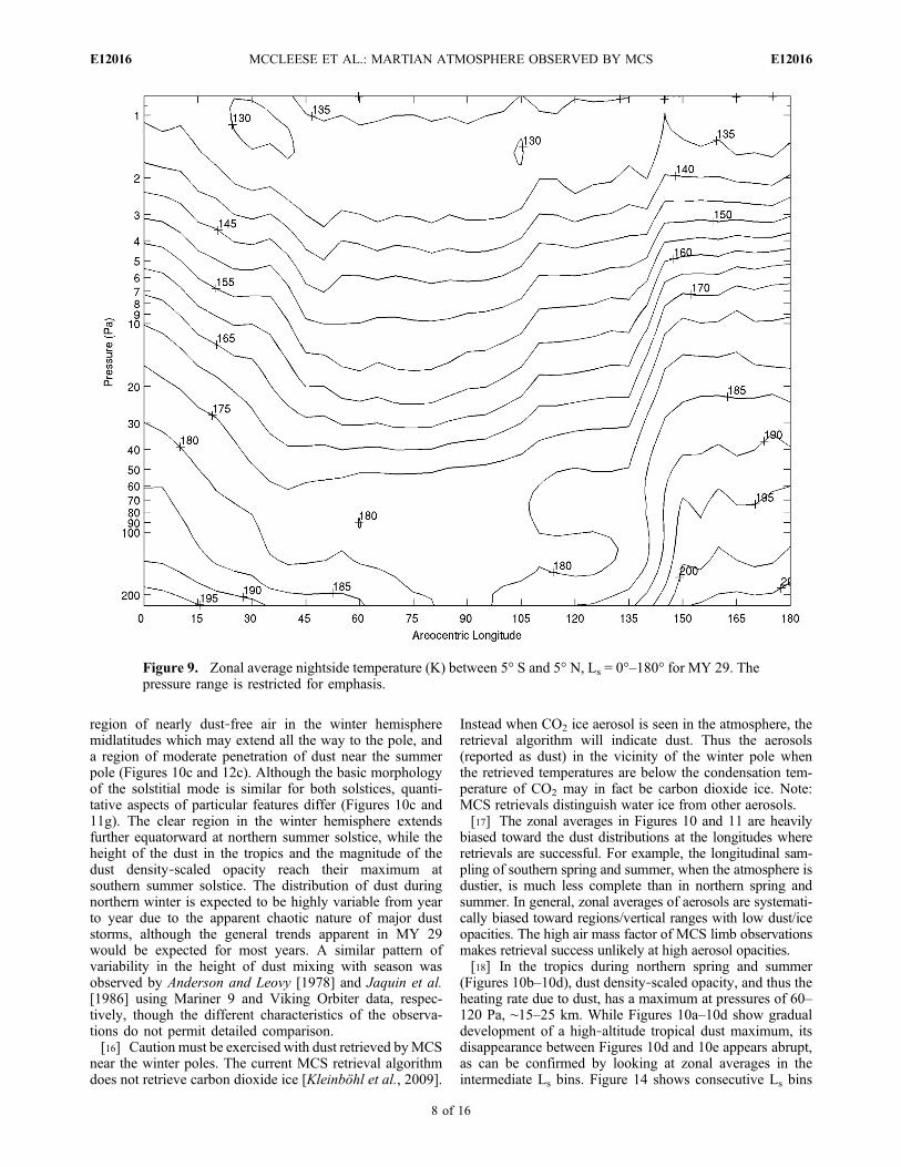
northern jet gradually decays to nothing at the northernsummer solstice and then grows back to its equinoctialintensity relatively gradually except for the abrupt changearound Ls = 140°–145°. The southern jet intensity also risesabruptly during this period. Figure 8b shows the differencebetween the southern and northern jet intensities at theirrespective maxima in comparison with a simple sinusoidwith an extremum at northern summer solstice. As expected,the difference in jet intensity is small at the equinoxes andvery large at the northern summer solstice.[14] Figure 9 shows the variation in equatorial nightside

thermal structure during northern spring and summer of MY29. Temperatures cool from their vernal equinox values to aminimum at ∼Ls = 45°, remain roughly constant until afternorthern summer solstice, and then gradually warm until Ls

= 135°. Beginning with Ls = 135°–145°, there is a moreabrupt rise in temperature (observe the slope of the iso-therms) of ∼1 K/degree of Ls over a great depth of themiddle atmosphere (2–90 Pa). Yet since the equator‐polegradient increases at roughly the same rate at both poles, thissudden warming at the equator does not affect the general

sinusoidal variation in the difference in jet intensities. Anabrupt change in temperatures in this latitudinal band andseason was not observed in MY 28.

3.2. Seasonal Variability of the Latitudinal VerticalDistribution of Dust

[15] Figures 10 and 11 show the seasonal variation of thezonal average of dust density‐scaled opacity (note the log10dimension of the color bar). We use the density‐scaledopacity (the quotient of opacity and the atmospheric density)to describe aerosol distribution because it is both propor-tional the mass mixing ratio and the aerosol heating rate.For reference, the zonal average dust opacity is plotted inFigure 12 (nightside) and Figure 13 (dayside). This quantityis proportional to the particle number density of dust. Thelatitudinal vertical distribution of dust has equinoctial andsolstitial modes. The equinoctial mode is characterized bypenetration of dust to high altitudes over the tropics and alower height of penetration near the poles (Figures 10a and12a). Similarly, the solstitial mode is characterized bypenetration of dust to high altitudes over the tropics, a

Figure 8. (a) Estimated maximum westerly jet velocity in the southern hemisphere (red solid line) andthe northern hemisphere (blue dashed line) during northern spring and summer of MY 29. (b) Differencebetween the maximum westerly jet velocities in the southern and northern hemispheres during northernspring and summer of MY 29 (blue solid line). Red dashed line is −20 + 110 × sin(Ls).


7 of 16

region of nearly dust‐free air in the winter hemispheremidlatitudes which may extend all the way to the pole, anda region of moderate penetration of dust near the summerpole (Figures 10c and 12c). Although the basic morphologyof the solstitial mode is similar for both solstices, quanti-tative aspects of particular features differ (Figures 10c and11g). The clear region in the winter hemisphere extendsfurther equatorward at northern summer solstice, while theheight of the dust in the tropics and the magnitude of thedust density‐scaled opacity reach their maximum atsouthern summer solstice. The distribution of dust duringnorthern winter is expected to be highly variable from yearto year due to the apparent chaotic nature of major duststorms, although the general trends apparent in MY 29would be expected for most years. A similar pattern ofvariability in the height of dust mixing with season wasobserved by Anderson and Leovy [1978] and Jaquin et al.[1986] using Mariner 9 and Viking Orbiter data, respec-tively, though the different characteristics of the observa-tions do not permit detailed comparison.[16] Caution must be exercised with dust retrieved byMCS

near the winter poles. The current MCS retrieval algorithmdoes not retrieve carbon dioxide ice [Kleinböhl et al., 2009].

Instead when CO2 ice aerosol is seen in the atmosphere, theretrieval algorithm will indicate dust. Thus the aerosols(reported as dust) in the vicinity of the winter pole whenthe retrieved temperatures are below the condensation tem-perature of CO2 may in fact be carbon dioxide ice. Note:MCS retrievals distinguish water ice from other aerosols.[17] The zonal averages in Figures 10 and 11 are heavily

biased toward the dust distributions at the longitudes whereretrievals are successful. For example, the longitudinal sam-pling of southern spring and summer, when the atmosphere isdustier, is much less complete than in northern spring andsummer. In general, zonal averages of aerosols are systemati-cally biased toward regions/vertical ranges with low dust/iceopacities. The high air mass factor of MCS limb observationsmakes retrieval success unlikely at high aerosol opacities.[18] In the tropics during northern spring and summer

(Figures 10b–10d), dust density‐scaled opacity, and thus theheating rate due to dust, has a maximum at pressures of 60–120 Pa, ∼15–25 km. While Figures 10a–10d show gradualdevelopment of a high‐altitude tropical dust maximum, itsdisappearance between Figures 10d and 10e appears abrupt,as can be confirmed by looking at zonal averages in theintermediate Ls bins. Figure 14 shows consecutive Ls bins

Figure 9. Zonal average nightside temperature (K) between 5° S and 5° N, Ls = 0°–180° for MY 29. Thepressure range is restricted for emphasis.


8 of 16

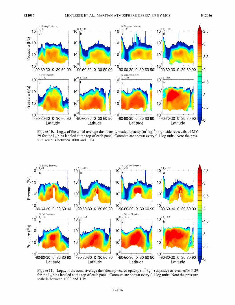
Figure 10. Log10 of the zonal average dust density‐scaled opacity (m2 kg−1) nightside retrievals of MY29 for the Ls bins labeled at the top of each panel. Contours are shown every 0.1 log units. Note the pres-sure scale is between 1000 and 1 Pa.

Figure 11. Log10 of the zonal average dust density‐scaled opacity (m2 kg−1) dayside retrievals of MY 29

for the Ls bins labeled at the top of each panel. Contours are shown every 0.1 log units. Note the pressurescale is between 1000 and 1 Pa.


9 of 16

Figure 12. Log10 of the zonal average dust opacity (km−1) nightside retrievals of MY 29 for the Ls binslabeled at the top of each panel. Contours are shown every 0.1 log units. Note the pressure scale isbetween 1000 and 1 Pa.

Figure 13. Log10 of the zonal average dust opacity (km−1) dayside retrievals of MY 29 for the Ls binslabeled at the top of each panel. Contours are shown every 0.1 log units. Note the pressure scale isbetween 1000 and 1 Pa.


10 of 16

between Ls = 130 to 165 for nightside zonal averages of dustdensity‐scaled opacity during middle‐to‐late northern sum-mer ofMY 29. Between Ls = 130° and Ls = 135° (Figures 14aand 14b), the vertical and latitudinal distribution of dust isvirtually unchanged. At Ls = 140° (Figure 14c), the high‐altitude tropical maximum shifts toward the southernhemisphere, but another maximum appears in the northerntropics at Ls = 145° (Figure 14d) and reaches a pressurelevel of ∼30 Pa (∼35 km). Figures 14f–14h show a morelatitudinally uniform maximum in density‐scaled opacityextending from 50°S to 50°N.[19] In an effort to deconvolve the spatial and temporal

variability of dust immediately following Ls = 130, we showin Figure 15 cross sections of dust density‐scaled opacityconstructed from retrievals from five nightside MRO passes.These cross sections were selected because they contain atleast one retrieval between 5° S and 5° N that crosses theequator in a narrow longitudinal band (170°–180° E) inmidnorthern summer (Ls = 127°–143°). These cross sectionsprovide snapshots over a short time interval of time of thedust distribution just west of the Martian dateline. Exam-ining Figure 15 at the equator, there is an abrupt change inthe vertical extent of the dust between Ls = 135° and 141°,the timeframe of the change seen in Figures 10d and 10e,although there is significant variability across all of theobservations comprising the cross sections. Furthermore, theindividual profiles show more varied spatial structure,including very sharp vertical variations in density‐scaledopacity, highlighting the importance of subscale height ob-servations (even MCS may be smoothing these structureseven at 5 km resolution).[20] Figures 15a–15c show a strong maximum in dust

mass mixing ratio at 60 Pa in the northern tropics. In the

interval between Figures 15c and 15d (6° of Ls, ∼12 sols),the top of the dusty region has descended, and the dustdensity‐scaled opacity at 60 Pa has fallen from near 10−3 tobelow 10−6 m2 kg−1. A few sols later (Figure 15e), much ofthe northern tropics has cleared, although a layer of dust isevident at a pressure level near ∼60 Pa (∼25 km). From thesouthern midlatitudes to tropics, conditions become muchdustier with time (by about 2 orders of magnitude at 100 Pa)between Figures 15b and 15d. However, dust in significantamounts is confined to north of 45°S. Note that a large spanof high southern of latitude is entirely dust free, down to atleast 200 Pa. Near the south pole, a layer of aerosol(retrieved as dust, but because it is the winter pole may beCO2 ice) emerges from the south pole extending equator-ward in Figure 15b.[21] Observations by the Mars Color Imager (MARCI) on

MRO and the Thermal Emission Spectrometer (THEMIS)on Mars Odyssey suggest that the changes in dust latitudinalvertical structure depicted in Figure 14 and 15 occur atnearly the same time as the initiation of a regional duststorm in the southern tropics and subtropics; a significantincrease in column optical depth is also observed in thetropics [Malin et al., 2008; Smith, 2009]. These dust eventsare all nearly simultaneous with the abrupt warming near theequator and the rapid increase in the intensities of the winterwesterly jets discussed in section 3.1, suggesting thesephenomena may be related.[22] A high‐altitude dust maximum is also present in the

southern extratropics during the middle of southern summer(Figures 10g and 11g) and is closer to the south pole innightside observations. During this time, a decayingregional dust storm and associated diffuse dust haze wasobserved in the southern midlatitudes by MARCI [Malin

Figure 14. Log10 of the zonal average dust density‐scaled opacity (m2 kg−1) nightside retrievals for theconsecutive Ls bins in MY 29 labeled at the top of each panel. Contours are shown every 0.1 log units.


11 of 16

et al., 2009]. The penetration of dust over the southernsummer pole is also striking; approximately 15–20 km higherthan over the north pole during the middle of northern sum-mer (Figures 10c–10d and 11c–11d).

3.3. Seasonal Variability of the Latitudinal VerticalDistribution of Water Ice

[23] Figures 16 and 17 show the seasonal variability in thezonal average of water ice density‐scaled opacity on boththe nightside and dayside. This quantity is proportional tothe mass mixing ratio of water ice. For reference, Figures 18and 19 show the zonal average water ice opacity. Water iceclouds are present throughout the year at various locationsover the planet, and continuously over the equator. Vari-ability between nightside and dayside averages is quitesignificant. Of particular note is the strong diurnal vari-

ability in tropical water ice during most seasons. Wilson andRichardson [2000] argued, based on Viking Lander ob-servations of cloud dissipation in late morning and their tidalmodel, that the vertical propagation of atmospheric tem-perature maxima and minima in the tropics is due to thediurnal tide might control cloud formation and dissipation.The basic principle is that if clouds condense at a given levelof the atmosphere, that level of the atmosphere must havehigh relative humidity and thus is likely a local temperatureminimum. Thus, as the temperature minimum propagatesvertically with the tide, clouds sublimate at the originalposition of the temperature minimum and condense in thenew position of the temperature minimum.[24] Caution must be exercised in interpreting the zonal

averages of water ice, due to the systematic bias favoringsuccessful retrievals. In addition, ice layers at high altitudes

Figure 15. Log10 of the dust density‐scaled opacity (m2 kg−1) in all available retrievals from five night-side MRO passes with available retrievals in a box bounded by 5° S–5°N, 170° E–180° E: (a) 15 Sep-tember 2008 (orbit numbers 10024–10025), mean Ls = 127.6085°; (b) 21 September 2008 (orbitnumbers 10103–10104), mean Ls = 130.5607°; (c) 2 October 2008 (orbit numbers 10235–10236), meanLs = 135.5447°; (d) orbit numbers 10393–10394, mean Ls = 141.6316°; (e) 14 October 2008 (orbit numb-ers 10446–10447), mean Ls = 143.6980°. The solid lines mark the mean latitude of the retrievals, andtheir lower end marks the highest pressure at which dust is reported. Contours are shown every 0.1log units.


12 of 16

Figure 16. Log10 of the zonal average water ice density‐scaled opacity (m2 kg−1) nightside retrievals ofMY 29 for the Ls bins labeled at the top of each panel. Contours are shown every 0.1 log units. Note thepressure scale is between 1000 and 0.1 Pa.

Figure 17. Log10 of the zonal average water ice density‐scaled opacity (m2 kg−1) dayside retrievals forMY 29 for the Ls bins labeled at the top of each panel. Contours shown are every 0.1 log units. Note thepressure scale is between 1000 and 0.1 Pa.


13 of 16

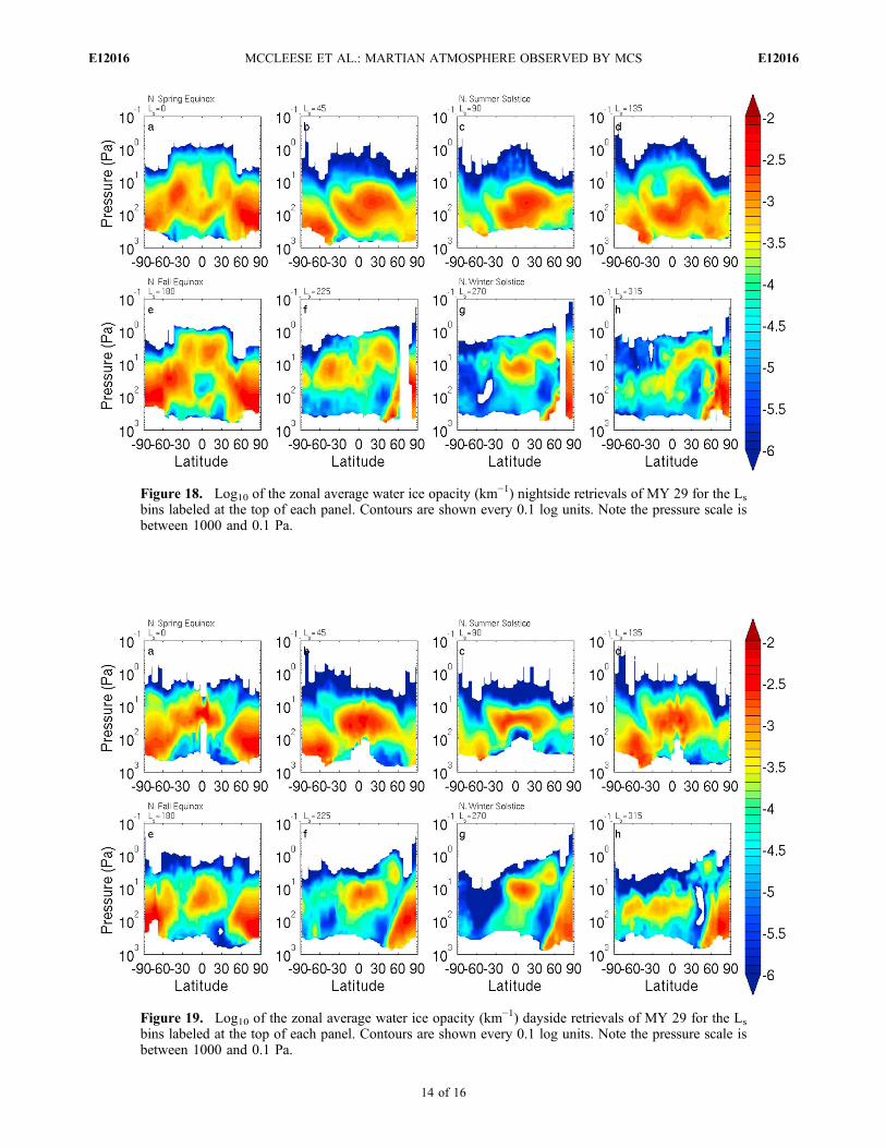
Figure 18. Log10 of the zonal average water ice opacity (km−1) nightside retrievals of MY 29 for the Ls

bins labeled at the top of each panel. Contours are shown every 0.1 log units. Note the pressure scale isbetween 1000 and 0.1 Pa.

Figure 19. Log10 of the zonal average water ice opacity (km−1) dayside retrievals of MY 29 for the Ls

bins labeled at the top of each panel. Contours are shown every 0.1 log units. Note the pressure scale isbetween 1000 and 0.1 Pa.


14 of 16

may be missed, especially when there is a layer of ice greatlydetached from a more significant layer lower in the atmo-sphere, since the top level at which water ice is retrieved isset by a radiance‐based criterion [Kleinböhl et al., 2009].[25] At northern spring equinox, water ice on the night-

side is distributed from 60° S to 90° N (Figure 16a) andextending from the bottom of MCS’s observable range to apressure level near 1 Pa (∼60 km). Multiple broad maximain the density‐scaled opacity is seen over these latitudesand pressures, with the largest values occurring at 15 Paand 40° S. On the dayside (Figure 17a), water ice is moretightly confined in latitude and extending over a narrowerrange of pressure. In addition, a well defined minimum inwater ice now separates the tropical water ice from thenorthern polar water ice. This minimum tilts from 30° N at100 Pa to 50° N at 5 Pa. A similar feature appears both in thenorth and south at many seasons, especially on the dayside.[26] Half a season later (Figures 16b and 17b), signifi-

cantly less water ice is seen at high latitudes, and the highestdensity‐scaled opacities on both the nightside and daysideare confined and centered at the equator. At northern summersolstice (Figures 16c and 17c), the basic pattern of Ls = 45°continues, though there is a clearing of ice at 60 Pa over theequator on the dayside. Again, a water ice minimum tiltingtoward the pole with lower pressure separates the tropicalwater ice from the polar water ice in dayside retrievals. Atthis season, past observations suggest the subtropical cloudbelt (called the “aphelion cloud belt” by some authors)reaches its zenith soon after northern summer solstice.[27] A half season later (Figures 16d and 17d), the

structure of the subtropical cloud belt has changed. The topof the ice clouds in the tropics is substantially higher. Waterice has increased at both poles, though the ice in thesouthern polar region is separated from the ice in the tropicsby a water ice minimum on the dayside. The increase innightside water ice below 100 Pa between Ls = 90°–135°observed by MCS at northern polar latitudes is consistentwith observations of a considerable increase in water iceclouds by the Mars Phoenix Lander at its landing site near70° N after ∼Ls = 111° [Whiteway et al., 2009].[28] The distribution of ice at the northern autumnal equi-

nox (Figures 16e and 17e) is similar to the distribution of iceat the northern vernal equinox (Figures 16a and 17a), exceptthe concentrations of water ice above 10 Pa on the nightsideare significantly greater. One explanation for this asymmetrybetween the equinoctial distributions is that there is no sea-sonal carbon dioxide ice cap over the north pole duringsummer, exposing the water ice cap and enhancing watervapor flux to the atmosphere in this season [Jakosky, 1985].[29] This asymmetry between north and south continues

throughout the remainder of the year (Figures 16f–16h and17f–17h). Water ice density‐scaled opacities are higher inthis period. The atmosphere at pressures higher than 80 Pain nightside observations is generally ice free from thesouthern pole to 60° N at Ls = 225° through Ls = 315°.

4. Summary

[30] We have described the seasonal variations of thezonal mean atmospheric fields, spanning more than a Mar-tian year, providing the first systematic mapping of thelower and middle atmosphere. This is the minimum extent

of the atmosphere necessary to properly represent thedynamics of the lower and middle atmosphere in generalcirculation models [Wilson, 1997; Forget et al., 1999].[31] The thermal structure of the atmosphere is shown in

MCS observations to vary seasonally between two modes: asymmetrical equinoctial structure with intense atmosphericpolar warming overlying polar vortices; and a solstitialstructure with a middle atmospheric warming over the winterpole, and a cold deep winter lower atmospheric polar vortex.[32] MCS has provided global and seasonal vertical pro-

files of aerosols (dust and water ice) at the same verticalresolution (∼5 km) as the retrieved temperature profiles.These profiles reveal unanticipated characteristics in theaerosol distributions. For dust, the observations show avertical distribution during some seasons that significantlydeviates from an idealized profile constructed from thebalance between sedimentation and vertical eddy diffusion[Conrath, 1975]. While the lowest reaches of the atmo-sphere are dustier than those of the middle atmosphere, thevertical dust distribution during most of northern spring andsummer appears to contain a maximum in dust mass mixingratio away from the surface. At roughly 15–25 km abovethe surface, above the maximum boundary layer depth, theexistence of this maximum suggests that current under-standing of the mechanisms by which dust enters and leavesthe atmosphere is incomplete.[33] Dust profiles from MCS also reveal in unprecedented

detail considerable complexity and significant temporal andspatial variability of the dust distribution. Multiple layers ofdust can be seen in cross sections of MCS data. The dustprofiles also show that the atmosphere can be nearly dustfree in certain regions and seasons.[34] MCS observations yield the first vertically resolved,

seasonal mapping of the distribution of atmospheric waterice. The retrieved profiles show water ice cross sectionswhose vertical and latitudinal distribution varies signifi-cantly with both the seasonal and diurnal cycles. The diurnalcycle variation is largely a product of the temperature var-iations associated with the strong diurnal tide. Indeed, Leeet al. [2009] and Benson et al. [2010] have used MCS datato show that the diurnal variation in ice opacity distributioncorrespond with diurnal temperature variations, which inturn show a pattern very close to that predicted for thevertically propagating tide. Seasonal variations reflect thevariation of both water vapor and thermal structure. Ingeneral, the tropical water ice cloud is higher and thedensity‐scaled opacity greater in southern summer than innorthern summer. The higher cloud in the southern summeratmosphere is associated with the much warmer temper-atures, and the cloud base and top are generally separatedby a roughly order of magnitude in pressure, yielding anextended vertical haze. Near the solstices, the cloud beltextends horizontally throughout the tropics and into thelower midlatitudes. A well‐defined break or clearing ofwater ice opacity occurs between mid latitudes and thewinter pole.

[35] Acknowledgments. We would like to thank Tina Pavlicek forher contributions to MCS instrument operations and Mark Apolinskifor his work on processing the MCS data. We also wish to thank WayneHartford and Mark Foote for their contributions to the design and fabrica-tion of the instrument and the MRO spacecraft operations teams who make


15 of 16

this investigation possible. Work at the Jet Propulsion Laboratory, Califor-nia Institute of Technology, was performed under a contract with NASA.

ReferencesAnderson, E., and C. Leovy (1978), Mariner 9 television limb observationsof dust and ice hazes on Mars, J. Atmos. Sci., 35(4), 723–734.

Benson, J. L., D. M. Kass, A. Kleinböhl, D. J. McCleese, J. T. Schofield,and F. W. Taylor (2010), Mars’ south polar hood as observed by theMars Climate Sounder, J. Geophys. Res., doi:10.1029/2009JE003554,in press.

Clancy, R. T., B. J. Sandor, M. J. Wolff, P. R. Christensen, M. D. Smith,J. C. Pearl, B. J. Conrath, and R. J. Wilson (2000), An intercomparisonof ground‐based millimeter, MGS TES, and Viking atmospheric temper-ature measurements: Seasonal and interannual variability of tempera-tures and dust loading in the global Mars atmosphere, J. Geophys.Res., 105(E4), 9553–9571.

Conrath, B. J. (1975), Thermal structure of the Martian atmosphere duringthe dissipation of the dust storm of 1971, Icarus, 24, 36–46.

Conrath, B. J., J. C. Pearl, M. D. Smith, W. C. Maguire, P. R. Christensen,S. Dason, and M. S. Kaelberer (2000), Mars Global Surveyor ThermalEmission Spectrometer (TES) observations: Atmospheric temperaturesduring aerobraking and science phasing, J. Geophys. Res., 105(E4),9509–9519, doi:10.1029/1999JE001095.

Forget, F., F. Hourdin, R. Fournier, C. Hourdin, O. Talagrand, M. Collins,S. R. Lewis, P. L. Read, and J.‐P. Huot (1999), Improved general circu-lation models of the Martian atmosphere from the surface to above 80km, J. Geophys. Res., 104, 24,155–24,175.

Forget, F., F. Montmessin, J.‐L. Bertaux, F. Gonzalez‐Galindo, S. Lebonnois,E. Quemerais, A. Reberac, E. Dimarellis, and M. A. Lopez Valverde(2009), The density and temperatures of the upper Martian atmospheremeasured by stellar occultations with Mars Express SPICAM, J. Geophys.Res., 114, E01004, doi:10.1029/2008JE003086.

French, R. G., and P. J. Gierasch (1979), The Martian polar vortex: Theoryof seasonal variation and observations of Eolian features, J. Geophys.Res., 84(B9), 4634–4642, doi:10.1029/JB084iB09p04634.

Hinson, D. P., M. D. Smith, and B. J. Conrath (2004), Comparison of atmo-spheric temperatures obtained through infrared sounding and radio occul-tation by Mars Global Surveyor, J. Geophys. Res., 109, E12002,doi:10.1029/2004JE002344.

Holton, J. R. (2004), An Introduction to Dynamic Meteorology, 4th ed., 535pp., Elsevier, Amsterdam.

Jakosky, B. M. (1985), The seasonal cycle of water on Mars, Space Sci.Rev., 41(1–2), 131–200, doi:10.1007/BF00241348.

Jaquin, F., P. Gierasch, and R. Kahn (1986), The vertical structure of limbhazes in the Martian atmosphere, Icarus, 72, 528–534.

Keating, G. M., et al. (1998) The structure of the upper atmosphere ofMars: In situ accelerometer measurements from Mars Global Surveyor,Science, 13, 1672–1676, doi:10.1126/science.

Kleinböhl, A., et al. (2009), Mars Climate Sounder limb profile retrieval ofatmospheric temperature, pressure, dust, and water ice opacity, J. Geo-phys. Res., 114, E10006, doi:10.1029/2009JE003358.

Lee, C., et al. (2009), Thermal tides in the Martian middle atmosphere asseen by the Mars Climate Sounder, J. Geophys. Res., 114, E03005,doi:10.1029/2008JE003285.

Malin, M. C., B. A. Cantor, D. E. Shean, M. R. Kennedy, and T. N.Harrison (2008), MRO MARCI weather report for the week of 3November 2008–9 November 2008, Captioned Image Release,MSSS‐58, Malin Space Sci. Syst., San Diego, Calif. (Available athttp://www.msss.com/msss_images/2008/11/12/.)

Malin, M. C., B. A. Cantor, M. R. Kennedy, D. E. Shean, and T. N. Harrison(2009), MRO MARCI weather report for the week of 27 July 2009–2August 2009, Captioned Image Release, MSSS‐94, Malin Space Sci.Syst., San Diego, Calif. (Available at http://www.msss.com/msss_images/2009/08/05/.)

McCleese, D. J., J. T. Schofield, F. W. Taylor, S. B. Calcutt, M. C. Foote,D. M. Kass, C. B. Leovy, D. A. Paige, P. L. Read, and R. W. Zurek(2007), Mars Climate Sounder: An investigation of thermal and watervapor structure, dust and condensate distributions in the atmosphere,and energy balance of the polar regions, J. Geophys. Res., 112,E05S06, doi:10.1029/2006JE002790.

McCleese, D. J., et al. (2008), Intense polar temperature inversion in themiddle atmosphere on Mars, Nat. Geosci., 1, 745–749, doi:10.1038/ngeo332.

Smith, M. D. (2004), Interannual variability in TES atmospheric observa-tions of Mars during 1999–2003, Icarus, 167, 148–165.

Smith, M. D. (2009), THEMIS observations of Mars aerosol optical depthfrom 2002–2008, Icarus, 202(2), 444–452, doi:10.1016/j.icarus.2009.03.027.

Smith, M. D., J. C. Pearl, B. J. Conrath, and P. R. Christensen (2001), Ther-mal Emission Spectrometer results: Mars atmospheric thermal structureand aerosol distribution, J. Geophys. Res., 106, 23,929–23,945.

Whiteway, J. A., et al. (2009), Mars water‐ice clouds and precipitation,Science, 325(5936), 68–70, doi:10.1126/science.1172344.

Wilson, R. J. (1997), A general circulation model simulation of the Martianpolar warming, Geophys. Res. Lett., 24(2), 123–126.

Wilson, R. J., and M. I. Richardson (2000), The Martian atmosphere duringthe Viking mission, I: Infrared measurements of atmospheric tempera-tures revisited, Icarus, 145, 555–579.

Zurek, R. W., and S. E. Smrekar (2007), An overview of the Mars Recon-naissance Orbiter (MRO) science mission, J. Geophys. Res., 112,E05S01, doi:10.1029/2006JE002701.

W. A. Abdou, D. M. Kass, A. Kleinböhl, D. J. McCleese, J. T. Schofield,J. H. Shirley, and R. W. Zurek, Jet Propulsion Laboratory, CaliforniaInstitute of Technology, Pasadena, CA 91109, USA.J. L. Bandfield, Department of Atmospheric Sciences, University of

Washington, Seattle, WA 98195, USA.S. B. Calcutt, P. G. J. Irwin, P. L. Read, F. W. Taylor, and N. Teanby,

Department of Physics, University of Oxford, Oxford OX1 3PU, UK.N. G. Heavens, Division of Geological and Planetary Sciences,

California Institute of Technology, Pasadena, CA 91125, USA.S. R. Lewis, Department of Physics and Astronomy, Open University,

Milton Keynes MK7 6AA, UK.D. A. Paige, Department of Earth and Space Sciences, University of

California, Los Angeles, CA 90095, USA.M. I. Richardson, Ashima Research, 600 South Lake Ave., Ste. 303,

Pasadena, CA 91106, USA.


16 of 16

structure and dynamics of the martian lower and middle

Documents